autocorrelation and crosscorrelation in matlab

School of Communications Technology and Mathematical Sciences

Digital Signal Processing

Part 3Discrete-Time Signals & Systems Case Studies

S R Taghizadeh <[email protected]>

January 2000

Digital Signal Processing Case StudyCopyright-�S.R.Taghizadeh

2

IntroductionMatlab and its applications in analysis of continuous-time signals and systems has

been discussed in part 1 and 2 of this series of practical manuals. The purpose of part

3 is to discuss the way Matlab is used in analysis of discrete-time signals and systems.

Each section provides a series of worked examples followed by a number of

investigative problems. You are required to perform each of the worked examples in

order to get familiar to the concept of Matlab environment and its important functions.

In order to test your understanding of the concept of discrete-time signals & systems

analysis, you are required to complete as many of the investigation / case study

problems as possible. The areas covered are designed to enforce some of the topics

covered in the formal lecture classes. These are:

� Signal Generation and Presentation

� Discrete Fourier Transform

� Spectral analysis

� Autocorrelation and Cross correlation

� Time delay estimation


3

Signal Generation and ManipulationSinusoidal Signal Generation

Consider generating 64 samples of a sinusoidal signal of frequency 1KHz, with a

sampling frequency of 8KHz.

A sampled sinusoid may be written as:

)2sin()( �� nffAnxs

where f is the signal frequency, fs is the sampling frequency, � is the phase and A is

the amplitude of the signal. The program and its output is shown below:

% Program: W2E1b.m% Generating 64 samples of x(t)=sin(2*pi*f*t) with a% Frequency of 1KHz, and sampling frequency of 8KHz.N=64; % Define Number of samplesn=0:N-1; % Define vector n=0,1,2,3,...62,63f=1000; % Define the frequencyfs=8000; % Define the sampling frequencyx=sin(2*pi*(f/fs)*n); % Generate x(t)plot(n,x); % Plot x(t) vs. tgrid;title('Sinewave [f=1KHz, fs=8KHz]');xlabel('Sample Number');ylabel('Amplitude');

0 10 20 30 40 50 60 70-1

-0.8

-0.6

-0.4

-0.2

0

0.2

0.4

0.6

0.8

1Sinewave [f=1KHz, fs=8KHz]

Sample Number

Am

plitu

de


4

Note that there are 64 samples with sampling frequency of 8000Hz or sampling time

of 0.125 mS (i.e. 1/8000). Hence the record length of the signal is 64x0.125=8mS.

There are exactly 8 cycles of sinewave, indicating that the period of one cycle is 1mS

which means that the signal frequency is 1KHz.

Task: Generate the following signals

(i) 64 Samples of a cosine wave of frequency 25Hz , sampling frequency 400Hz,

amplitude of 1.5 volts and phase =0.

(ii) The same signal as in (i) but with a phase angle of �/4 (i.e. 45o).

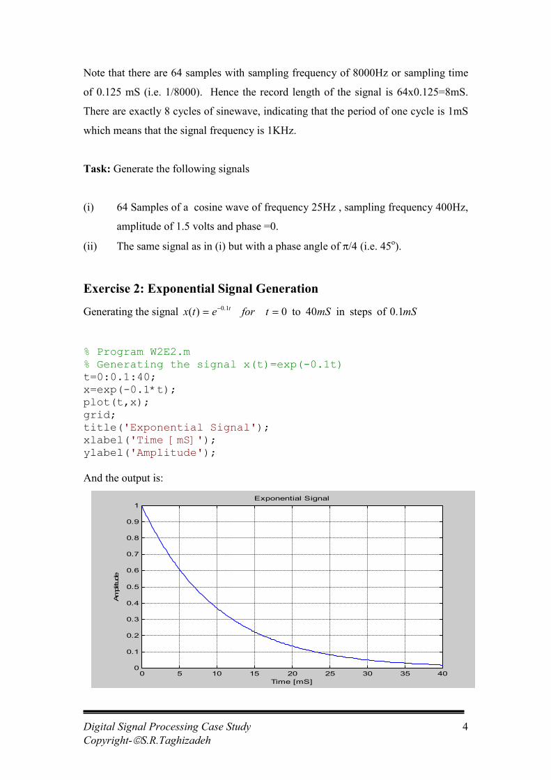
Exercise 2: Exponential Signal Generation

Generating the signal mSmStforetx t 1.0 of stepsin 40 to0 )( 1.0��

�

% Program W2E2.m% Generating the signal x(t)=exp(-0.1t)t=0:0.1:40;x=exp(-0.1*t);plot(t,x);grid;title('Exponential Signal');xlabel('Time [mS]');ylabel('Amplitude');

And the output is:

0 5 10 15 20 25 30 35 400

0.1

0.2

0.3

0.4

0.5

0.6

0.7

0.8

0.9

1Exponential Signal

Time [mS]

Am

plitu

de


5

Task: Generate the signal: Sec 0.1 of stepsin 40ms to0for t )6.0sin()( 1.0��

� tetx t

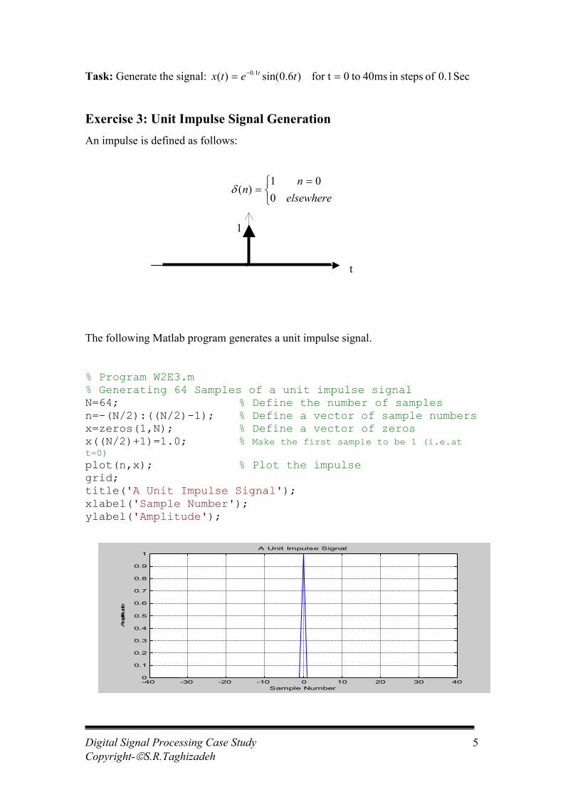
Exercise 3: Unit Impulse Signal GenerationAn impulse is defined as follows:

��

�elsewhere

nn

001

)(�

The following Matlab program generates a unit impulse signal.

% Program W2E3.m% Generating 64 Samples of a unit impulse signalN=64; % Define the number of samplesn=-(N/2):((N/2)-1); % Define a vector of sample numbersx=zeros(1,N); % Define a vector of zerosx((N/2)+1)=1.0; % Make the first sample to be 1 (i.e.att=0)plot(n,x); % Plot the impulsegrid;title('A Unit Impulse Signal');xlabel('Sample Number');ylabel('Amplitude');

-40 -30 -20 -10 0 10 20 30 400

0.1

0.2

0.3

0.4

0.5

0.6

0.7

0.8

0.9

1A Unit Impulse Signal

Sample Number

Amplitude

t

1


6

Task: Generate 40 samples of the following signals:

(for n=-20,-19,-18,…,0,1,2,3,…,18,19)

(i) x(n)=2�(n-10)

(ii) x(n)=5�(n-10)+2.5�(n-20)

Exercise 4: Unit Step Signal GenerationA step signal is defined as follows:

��

�otherwise

nnu

001

)(

The following Matlab Program generates and plots a unit step signal:

% Program: W2E4.m% Generates 40 samples of a unit step signal, u(n)N=40; % Define the number of samplesn=-20:20; % Define a suitable discrete time axisu=[zeros(1,(N/2)+1),ones(1,(N/2))]; % Generate thesignalplot(n,u); % Plot the signalaxis([-20,+20,-0.5,1.5]); % Scale axisgrid;title('A Unit Step Signal');xlabel('Sample Number');ylabel('Amplitude');

-20 -15 -10 -5 0 5 10 15 20-0.5

0

0.5

1

1.5A Unit Step Signal

Sample Number

Am

plitu

de

Digital Signal ProcesCopyright-�S.R.Tagh

Task: Generate 40 samples of each of the following signals using an appropriate

discrete time scale:

(i) x(n)=u(n)-u(n-1)

(ii) g(n)=u(n-1)-u(n-5)

Exercise 5: Generating Random SignalsRandom number generators are useful in signal processing for testing and evaluating

various signal processing algorithms. For example, in order to simulate a particular

noise cancellation algorithm (technique), we need to create some signals which is

contaminated by noise and then apply this signal to the algorithm and monitor its

output. The input/ output spectrum may then be used to examine and measure the

performance of noise canceller algorithm. Random numbers are generated to

represent the samples of some noise signal which is then added to the samples of

some the wanted signal to create an overall noisy signal. The situation is demonstrated

by the following diagram.

Matlab provides two c

Normally Distributed

randn(N)

Is an N-by-N matrix w

mean zero and varianc

randn(M,N), and rand

++

Output,s(n)=x(n)+w(n)

Input, x(n)

Noise

NoiseCancellation

Output,y(n)�x(n)
�
sing Case Studyizadeh

7

ommands, which may be applied to generate random numbers.

Random Numbers.

ith random entries, chosen from a normal distribution with

e one.

n([M,N]) are M-by-N matrices with random entries.

, w(n)

algorithm


8

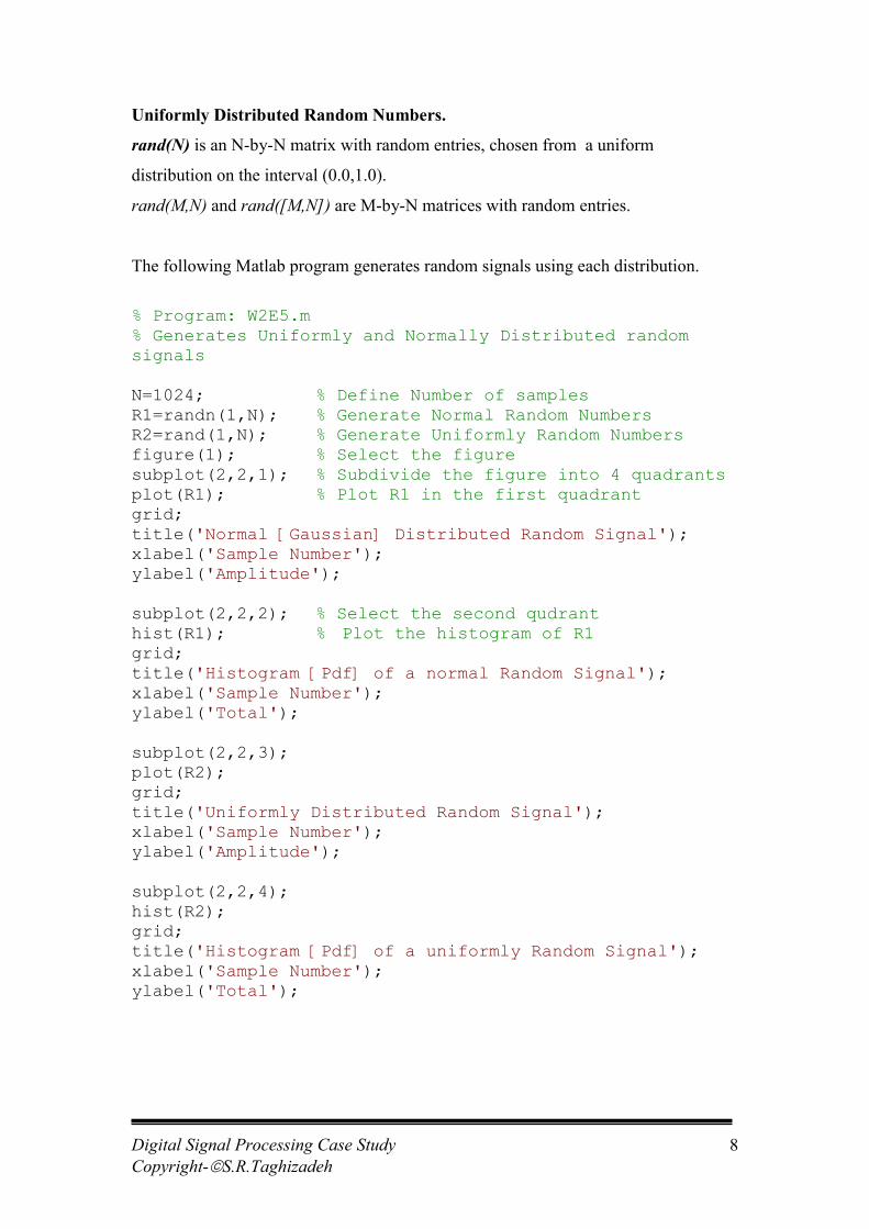
Uniformly Distributed Random Numbers.

rand(N) is an N-by-N matrix with random entries, chosen from a uniform

distribution on the interval (0.0,1.0).

rand(M,N) and rand([M,N]) are M-by-N matrices with random entries.

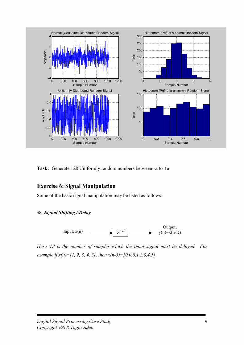
The following Matlab program generates random signals using each distribution.

% Program: W2E5.m% Generates Uniformly and Normally Distributed randomsignals

N=1024; % Define Number of samplesR1=randn(1,N); % Generate Normal Random NumbersR2=rand(1,N); % Generate Uniformly Random Numbersfigure(1); % Select the figuresubplot(2,2,1); % Subdivide the figure into 4 quadrantsplot(R1); % Plot R1 in the first quadrantgrid;title('Normal [Gaussian] Distributed Random Signal');xlabel('Sample Number');ylabel('Amplitude');

subplot(2,2,2); % Select the second qudranthist(R1); % Plot the histogram of R1grid;title('Histogram [Pdf] of a normal Random Signal');xlabel('Sample Number');ylabel('Total');

subplot(2,2,3);plot(R2);grid;title('Uniformly Distributed Random Signal');xlabel('Sample Number');ylabel('Amplitude');

subplot(2,2,4);hist(R2);grid;title('Histogram [Pdf] of a uniformly Random Signal');xlabel('Sample Number');ylabel('Total');


Task: Generate 128 Uniformly random numbers between -� to +�

Exercise 6: Signal ManipulationSome of the basic signal manipulation may be listed as follows:

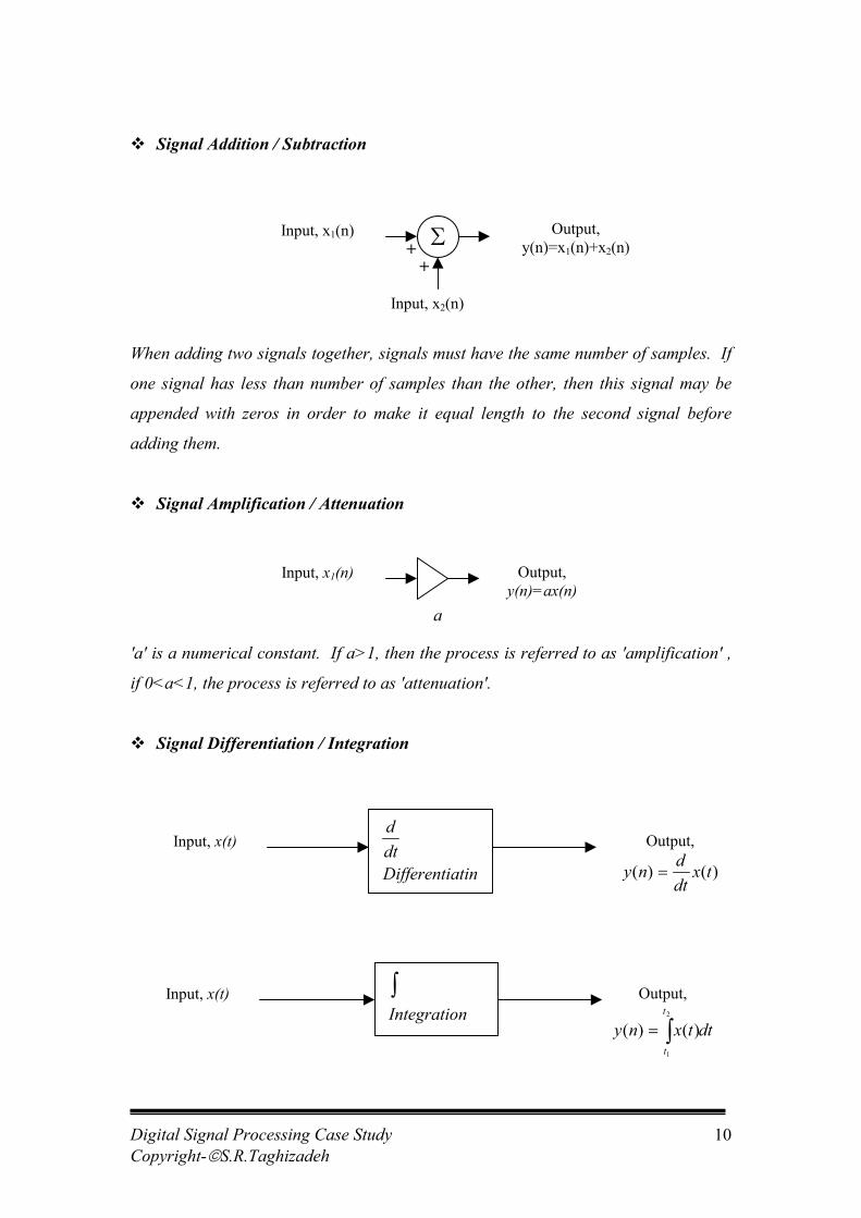
� Signal Shifting / Delay

Here 'D' is the number of samples w

example if x(n)=[1, 2, 3, 4, 5], then x(n

0 200 400 600 800 1000 1200-4

-2

0

2

4Normal [Gaussian] Distributed Random Signal

Sample Number

Am

plitu

de

-4 -2 0 2 40

50

100

150

200

250

300Histogram [Pdf] of a normal Random Signal

Sample Number

Tota

l

0 200 400 600 800 1000 12000

0.2

0.4

0.6

0.8

1Uniformly Distributed Random Signal

Sample Number

Am

plitu

de

0 0.2 0.4 0.6 0.8 10

50

100

150Histogram [Pdf] of a uniformly Random Signal

Sample Number

Tota

l

DZ �Input, x(n)Output,

y(n)=x(n-D)

9

hich the input signal must be delayed. For

-3)=[0,0,0,1,2,3,4,5].


10

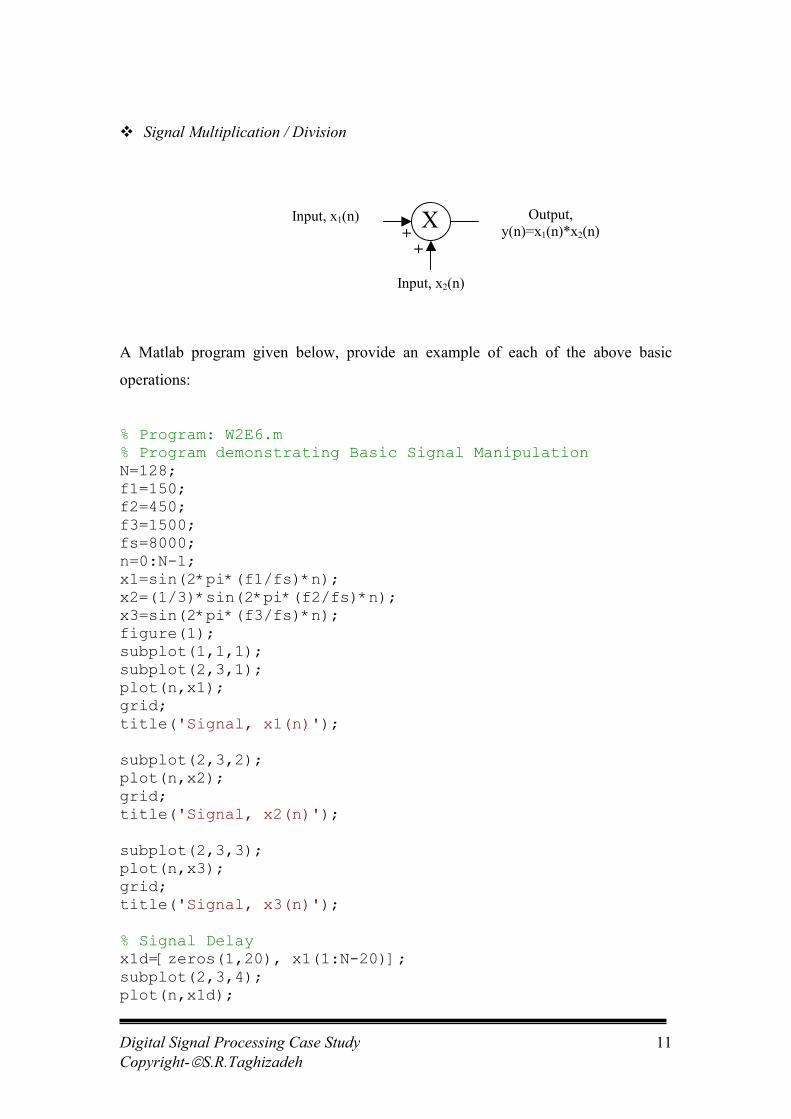
� Signal Addition / Subtraction

When adding two signals together, signals must have the same number of samples. If

one signal has less than number of samples than the other, then this signal may be

appended with zeros in order to make it equal length to the second signal before

adding them.

� Signal Amplification / Attenuation

'a' is a numerical constant. If a>1, then the process is referred to as 'amplification' ,

if 0<a<1, the process is referred to as 'attenuation'.

� Signal Differentiation / Integration

a

�

++

Output,y(n)=x1(n)+x2(n)

Input, x1(n)

Input, x2(n)

Input, x1(n) Output,y(n)=ax(n)

atinDifferentidtd

Input, x(t) Output,

)()( txdtdny �

nIntegratio�Input, x(t) Output,

dttxnyt

t��

2

1

)()(


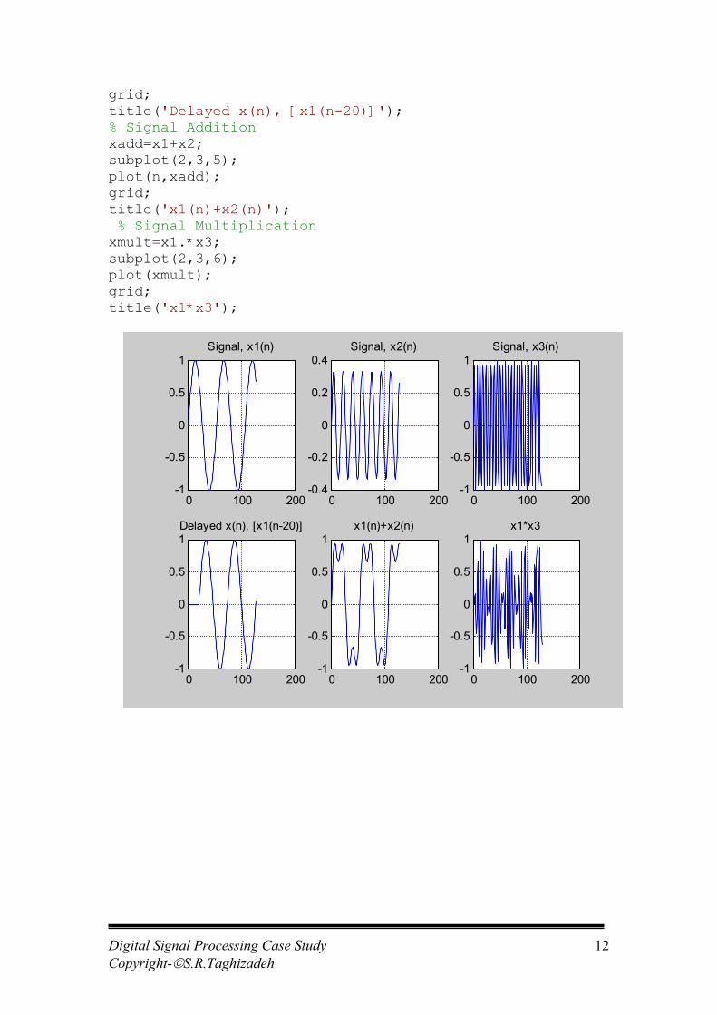
� Signal Multiplication / Division

A Matlab program given below, provide an

operations:

% Program: W2E6.m% Program demonstrating Basic SN=128;f1=150;f2=450;f3=1500;fs=8000;n=0:N-1;x1=sin(2*pi*(f1/fs)*n);x2=(1/3)*sin(2*pi*(f2/fs)*n);x3=sin(2*pi*(f3/fs)*n);figure(1);subplot(1,1,1);subplot(2,3,1);plot(n,x1);grid;title('Signal, x1(n)');

subplot(2,3,2);plot(n,x2);grid;title('Signal, x2(n)');

subplot(2,3,3);plot(n,x3);grid;title('Signal, x3(n)');

% Signal Delayx1d=[zeros(1,20), x1(1:N-20)];subplot(2,3,4);plot(n,x1d);

+Output,

y(n)=x (n)*x (n)Input, x1(n)

Inp

X

11

example of each of the above basic

ignal Manipulation

+1 2

ut, x2(n)


12

grid;title('Delayed x(n), [x1(n-20)]');% Signal Additionxadd=x1+x2;subplot(2,3,5);plot(n,xadd);grid;title('x1(n)+x2(n)'); % Signal Multiplicationxmult=x1.*x3;subplot(2,3,6);plot(xmult);grid;title('x1*x3');

0 100 200-1

-0.5

0

0.5

1Signal, x1(n)

0 100 200-0.4

-0.2

0

0.2

0.4Signal, x2(n)

0 100 200-1

-0.5

0

0.5

1Signal, x3(n)

0 100 200-1

-0.5

0

0.5

1Delayed x(n), [x1(n-20)]

0 100 200-1

-0.5

0

0.5

1x1(n)+x2(n)

0 100 200-1

-0.5

0

0.5

1x1*x3


13

Discrete Fourier Transform[1] Given a sampled signal x(n), its Discrete Fourier Transform (DFT) is given

by:

��

�

�

�

1

0

2N

n

N/nkje)n(x)k(X � k=0,1,2,…,N-1

The magnitude of the X(k) [i.e. the absolute value] against k is called the

spectrum of x(n). The values of k is proportional to the frequency of the

signal according to:

NkF

f sk �

Where Fs is the sampling frequency.

Assuming x is the samples of the signal of length N, then a simple Matlab

program to perform the above sum is shown below:

n=[0:1:N-1];k=[0:1:N-1];WN=exp(-j*2*pi/N);nk=n'*k;WNnk=WN .^ nk;Xk=x * WNnk;

Use the above routine to determine and plot the DFT of the following signal:

)tfcos()tfcos()t(x 21 22 ��

where

128N and ,HzF with,Hzf and Hzf s2 �� 800040010001

Note: Plot the magnitude and phase of Xk as follows:

MagX=abs(Xk);

PhaseX=angle(Xk)*180/pi;

figure(1);


14

subplo(2,1,1);

plot(k,MagX);

subplot(2,1,2);

plot(k,PhaseX);

Investigate:

(i) At what value of the index k does the magnitude of the DFT of x has major

peaks.

(ii) What is the corresponding frequency of the two peaks.

(iii) Perform the above for N=32, 64 and 512.

(iv) Comment on the results

(v) Set 128 and generate x(n) for n=0,1,2,…,N-1. Append a further 512 zeros to

x(n) as shown below: [Note the number of samples, N=128+512=640].

Xe=[x, zeros(1,512)];

Perform the DFT of the new sequence and plot its magnitude and phase.

Compare with the previous result. Explain the effect of zero padding a signal

with zero before taking the discrete Fourier Transform.

[2] Inverse DFT is defined as:

1-Nn0for )(1)(1

0

/2��

�

�

N

k

NnkjekXN

nx �

A simple Matlab routine to perform the inverse DFT may be written as

follows:

n=[0:1:N-1];k=[0:1:N-1];WN=exp(-j*2*pi/N);nk=n'*k;WNnk=WN .^ (-nk);x=(Xk * WNnk)/N;


15

Use x(n)={1,1,1,1}, and N=4, determine the DFT. Record the Magnitude and

phase of the DFT.

Use the IDFT to transfer the DFT results (i.e. Xk sequence) to its original

sequence.

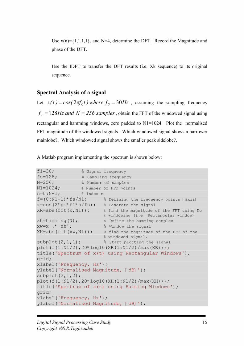
Spectral Analysis of a signal

Let Hzf where)tfcos()t(x 0 302 0 �� , assuming the sampling frequency

samples256N and Hzf s ��128 , obtain the FFT of the windowed signal using

rectangular and hamming windows, zero padded to N1=1024. Plot the normalised

FFT magnitude of the windowed signals. Which windowed signal shows a narrower

mainlobe?. Which windowed signal shows the smaller peak sidelobe?.

A Matlab program implementing the spectrum is shown below:

f1=30; % Signal frequencyfs=128; % Sampling frequencyN=256; % Number of samplesN1=1024; % Number of FFT pointsn=0:N-1; % Index nf=(0:N1-1)*fs/N1; % Defining the frequency points [axis]x=cos(2*pi*f1*n/fs); % Generate the signalXR=abs(fft(x,N1)); % find the magnitude of the FFT using No

% windowing (i.e. Rectangular window)xh=hamming(N); % Define the hamming samplesxw=x .* xh'; % Window the signalXH=abs(fft(xw,N1)); % find the magnitude of the FFT of the

% windowed signal.subplot(2,1,1); % Start plotting the signalplot(f(1:N1/2),20*log10(XR(1:N1/2)/max(XR)));title('Spectrum of x(t) using Rectangular Windows');grid;xlabel('Frequency, Hz');ylabel('Normalised Magnitude, [dB]');subplot(2,1,2);plot(f(1:N1/2),20*log10(XH(1:N1/2)/max(XH)));title('Spectrum of x(t) using Hamming Windows');grid;xlabel('Frequency, Hz');ylabel('Normalised Magnitude, [dB]');


16

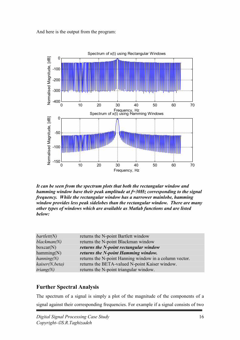
And here is the output from the program:

It can be seen from the spectrum plots that both the rectangular window andhamming window have their peak amplitude at f=30Hz corresponding to the signalfrequency. While the rectangular window has a narrower mainlobe, hammingwindow provides less peak sidelobes than the rectangular window. There are manyother types of windows which are available as Matlab functions and are listedbelow:

bartlett(N) returns the N-point Bartlett windowblackman(N) returns the N-point Blackman windowboxcar(N) returns the N-point rectangular windowhamming(N) returns the N-point Hamming window.hanning(N) returns the N-point Hanning window in a column vector.kaiser(N,beta) returns the BETA-valued N-point Kaiser window.triang(N) returns the N-point triangular window.

Further Spectral Analysis The spectrum of a signal is simply a plot of the magnitude of the components of a

signal against their corresponding frequencies. For example if a signal consists of two

0 10 20 30 40 50 60 70-400

-300

-200

-100

0Spectrum of x(t) using Rectangular Windows

Frequency, Hz

Nor

mal

ised

Mag

nitu

de, [

dB]

0 10 20 30 40 50 60 70-150

-100

-50

0Spectrum of x(t) using Hamming Windows

Frequency, Hz

Nor

mal

ised

Mag

nitu

de, [

dB]


17

sinusoidal at 120Hz and 60Hz, then ideally the spectrum would be a plot of

magnitude vs. frequency and would contain two peaks: one at 60 Hz and the other at

120 Hz illustrated in the next example. The following Matlab commands are the basis

of determining the spectrum of a signal:

fft

psd

spectrum

In the following examples, we illustrate their use. One of the most important aspects

of spectral analysis is the interpretation of the spectrum and its relation to the signal

under investigation.

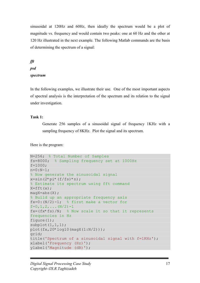
Task 1:

Generate 256 samples of a sinusoidal signal of frequency 1KHz with a

sampling frequency of 8KHz. Plot the signal and its spectrum.

Here is the program:

N=256; % Total Number of Samplesfs=8000; % Sampling frequency set at 1000Hzf=1000;n=0:N-1;% Now generate the sinusoidal signalx=sin(2*pi*(f/fs)*n);% Estimate its spectrum using fft commandX=fft(x);magX=abs(X);% Build up an appropriate frequency axisfx=0:(N/2)-1; % first make a vector forf=0,1,2,...(N/2)-1fx=(fx*fs)/N; % Now scale it so that it representsfrequencies in Hzfigure(1);subplot(1,1,1);plot(fx,20*log10(magX(1:N/2)));grid;title('Spectrum of a sinusoidal signal with f=1KHz');xlabel('Frequency (Hz)');ylabel('Magnitude (dB)');


18

And the output:

It is clear from the spectrum, that the signal consists of a single sinusoidal

components of frequency 1000Hz. Other artefacts in the figure are due to the limited

number of samples, windowing effects, and computation accuracy.

Task 1:

Consider, the notch filter in the previous section. The transfer function of the

notch filter is repeated here for convenience:

0 1000 2000 3000 4000-350

-300

-250

-200

-150

-100

-50

0

50Spectrum of a sinusoidal signal with f=1KHz

Frequency (Hz)

Mag

nitu

de (d

B)


19

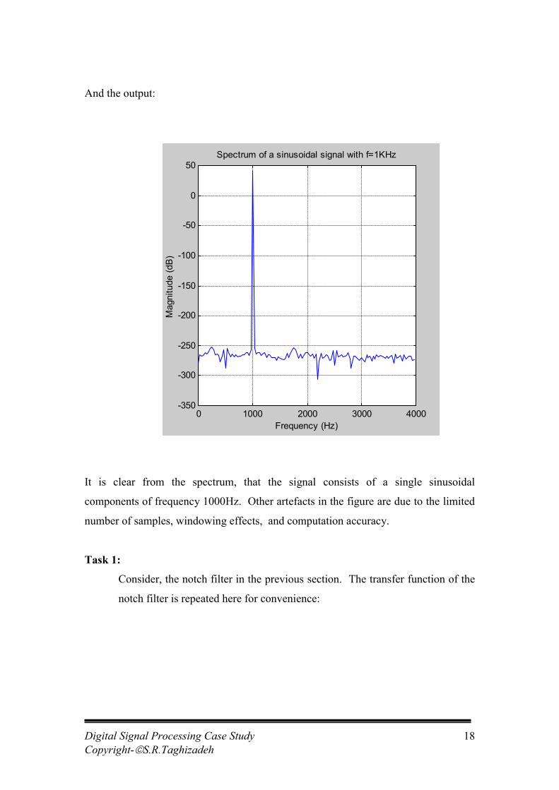
Apply an input signal:

)2sin()2sin()( 21

ss fnf

fnfnx ��

�� , with f1=120 Hz , f2=60 Hz and fs , the

sampling frequency at 1000Hz.

Plot the followings:

Input Spectrum

Magnitude response of the filter

Output Spectrum

Here is the Matlab Program:

% Program Name: Tut16.mclear;N=1024; % Total Number of Samplesfs=1000; % Sampling frequency set at 1000Hzf1=120;f2=60;n=0:N-1;x=sin(2*pi*(f1/fs)*n)+sin(2*pi*(f2/fs)*n);[pxx,fx]=psd(x,2*N,fs);plot(fx,20*log10(pxx));grid;title('Magnitude Spectrum of x(n)');xlabel('Frequency, Hz');ylabel('Magnitude, dB');sin(2*pi*(f2/fs)*n);b=[1 -1.8596 1];a=[1 -1.8537 0.9937];k=0.9969;b=k*b;figure(1);subplot(1,1,1);

subplot(1,3,1);

Output, y(n)Input, x(n)

21

21

9937.08537.118996.119969.0)(

��

��

��

��

zzzzzH

impulse response, h(n)


20

[pxx,fx]=psd(x,2*N,fs);plot(fx,20*log10(pxx));grid;title('Magnitude Spectrum of x(n)');xlabel('Frequency, Hz');ylabel('Magnitude, dB');

[h,f]=freqz(b,a,1024,fs); % Determines the frequency response% of

% the filter with coefficients 'b'% and 'a', using 1024 points around % the unit circle with a sampling

% frequency of fs. The function % returns the values of the transfer

% function h, for each frequency in % f in Hz. magH=abs(h); % Calculates the magnitude of the filterphaseH=angle(h); % Calculates the phase angle of the filtersubplot(1,3,2); % Divides the figure into two rows and one

% column and makes the first row the active% one

plot( f, 20*log10(magH)); % plots the magnitude in dB against % frequencygrid; % Add a grid

title('Magnitude Response of the Notch Filter');xlabel('Frequency');ylabel('Magnitude, dB');

y=filter(b,a,x);

[pyy,fy]=psd(y,2*N,fs); % determine the Spectrum using 'psd'subplot(1,3,3); % Select the third column in thefigureplot(fy,20*log10(pyy)); % Plot the output spectrum in dBgrid; % Add a gridtitle('Magnitude Spectrum of y(n)');xlabel('Frequency, Hz');ylabel('Magnitude, dB');

Here is the output from the program:


21

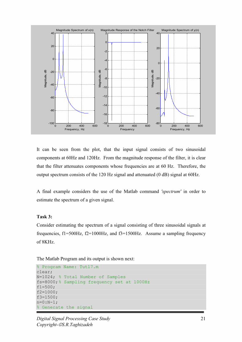
It can be seen from the plot, that the input signal consists of two sinusoidal

components at 60Hz and 120Hz. From the magnitude response of the filter, it is clear

that the filter attenuates components whose frequencies are at 60 Hz. Therefore, the

output spectrum consists of the 120 Hz signal and attenuated (0 dB) signal at 60Hz.

A final example considers the use of the Matlab command 'spectrum' in order to

estimate the spectrum of a given signal.

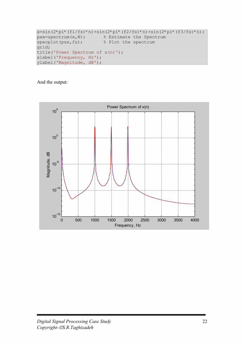
Task 3:

Consider estimating the spectrum of a signal consisting of three sinusoidal signals at

frequencies, f1=500Hz, f2=1000Hz, and f3=1500Hz. Assume a sampling frequency

of 8KHz.

The Matlab Program and its output is shown next:% Program Name: Tut17.mclear;N=1024; % Total Number of Samplesfs=8000;% Sampling frequency set at 1000Hzf1=500;f2=1000;f3=1500; n=0:N-1;% Generate the signal

0 200 400 600-100

-80

-60

-40

-20

0

20

40Magnitude Spectrum of x(n)

Frequency, Hz

Mag

nitu

de, d

B

0 200 400 600-18

-16

-14

-12

-10

-8

-6

-4

-2

0

2Magnitude Response of the Notch Filter

Frequency

Mag

nitu

de, d

B

0 200 400 600-80

-60

-40

-20

0

20

40Magnitude Spectrum of y(n)

Frequency, Hz

Mag

nitu

de, d

B


22

x=sin(2*pi*(f1/fs)*n)+sin(2*pi*(f2/fs)*n)+sin(2*pi*(f3/fs)*n);pxx=spectrum(x,N); % Estimate the Spectrum specplot(pxx,fs); % Plot the spectrumgrid;title('Power Spectrum of x(n)');xlabel('Frequency, Hz');ylabel('Magnitude, dB');

And the output:

0 500 1000 1500 2000 2500 3000 3500 400010-15

10-10

10-5

100

105Power Spectrum of x(n)

Frequency, Hz

Mag

nitu

de, d

B


23

Autocorrelation and Crosscorrelation in MatlabBoth in signal and Systems analysis, the concept of autocorrelation and

crosscorrelation play an important role. In the following sections, we present some

simple examples of how these two functions may be estimated in Matlab. The final

part of this section provides some applications of autocorrelation and crosscorrelation

functions in signal detection and time-delay estimations.

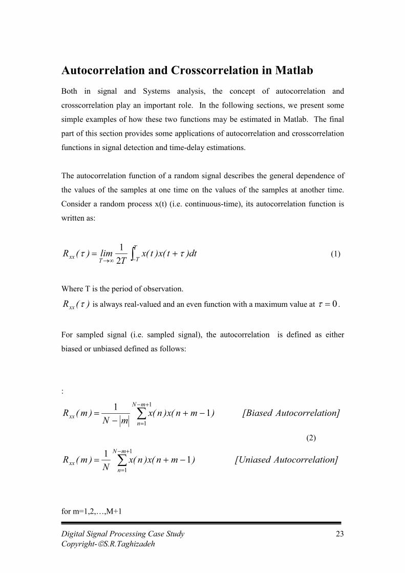
The autocorrelation function of a random signal describes the general dependence of

the values of the samples at one time on the values of the samples at another time.

Consider a random process x(t) (i.e. continuous-time), its autocorrelation function is

written as:

��

��

T

TTxx dt)t(x)t(xT

lim)(R ��

21

(1)

Where T is the period of observation.

)(Rxx � is always real-valued and an even function with a maximum value at 0�� .

For sampled signal (i.e. sampled signal), the autocorrelation is defined as either

biased or unbiased defined as follows:

:

ation]Autocorrel [Biased )mn(x)n(xmN

)m(RmN

nxx �

��

�

��

�

�

1

111

(2)

ation]Autocorrel [Uniased )mn(x)n(xN

)m(RmN

nxx �

��

�

��

1

111

for m=1,2,…,M+1


24

where M is the number of lags.

Some of its properties are listed in table 1.1.

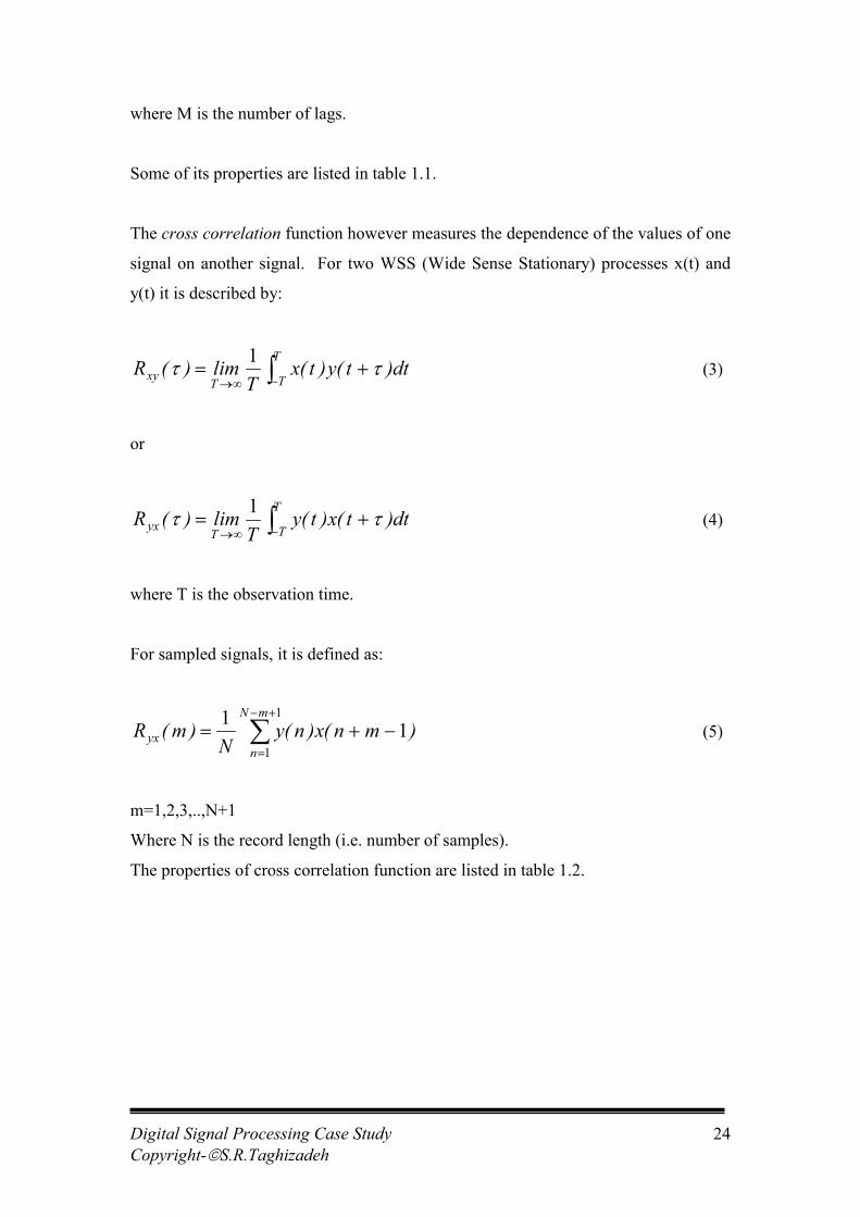
The cross correlation function however measures the dependence of the values of one

signal on another signal. For two WSS (Wide Sense Stationary) processes x(t) and

y(t) it is described by:

��

��

T

TTxy dt)t(y)t(xT

lim)(R ��

1(3)

or

��

��

T

TTyx dt)t(x)t(yT

lim)(R ��

1(4)

where T is the observation time.

For sampled signals, it is defined as:

��

�

��

1

111 mN

nyx )mn(x)n(y

N)m(R (5)

m=1,2,3,..,N+1

Where N is the record length (i.e. number of samples).

The properties of cross correlation function are listed in table 1.2.


25

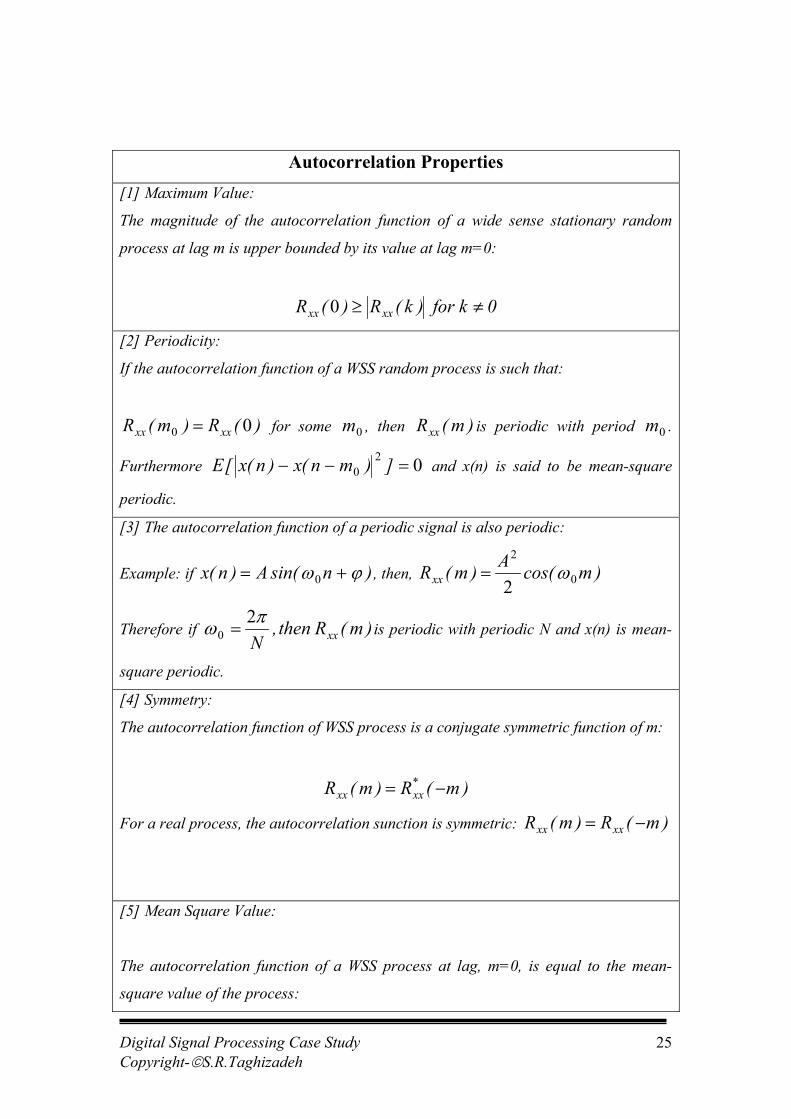
Autocorrelation Properties[1] Maximum Value:

The magnitude of the autocorrelation function of a wide sense stationary random

process at lag m is upper bounded by its value at lag m=0:

0k for )k(R)(R xxxx ��0

[2] Periodicity:

If the autocorrelation function of a WSS random process is such that:

)(R)m(R xxxx 00 � for some 0m , then )m(Rxx is periodic with period 0m .

Furthermore 020 �� ])mn(x)n(x[E and x(n) is said to be mean-square

periodic.

[3] The autocorrelation function of a periodic signal is also periodic:

Example: if )nsin(A)n(x �� 0 , then, )mcos(A)m(Rxx 0

2

2��

Therefore if )m(R then ,N xx�

�

20 � is periodic with periodic N and x(n) is mean-

square periodic.

[4] Symmetry:

The autocorrelation function of WSS process is a conjugate symmetric function of m:

)m(R)m(R *xxxx ��

For a real process, the autocorrelation sunction is symmetric: )m(R)m(R xxxx ��

[5] Mean Square Value:

The autocorrelation function of a WSS process at lag, m=0, is equal to the mean-

square value of the process:


26

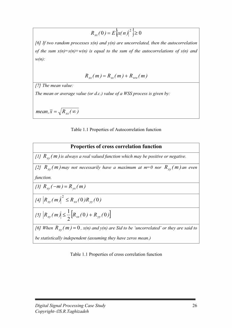
� � 00 2�� )n(xE)(Rxx

[6] If two random processes x(n) and y(n) are uncorrelated, then the autocorrelation

of the sum x(n)=s(n)+w(n) is equal to the sum of the autocorrelations of s(n) and

w(n):

)m(R)m(R)m(R wwssxx ��

[7] The mean value:

The mean or average value (or d.c.) value of a WSS process is given by:

)(Rx,mean xx ��

Table 1.1 Properties of Autocorrelation function

Properties of cross correlation function

[1] )m(Rxy is always a real valued function which may be positive or negative.

[2] )m(Rxy may not necessarily have a maximum at m=0 nor )m(Rxy an even

function.

[3] )m(R)m(R yxxy ��

[4] )(R)(R)m(R yyxxxy 002�

[5] � �)(R)(R)m(R yyxxxy 0021

��

[6] When 0�)m(Rxy , x(n) and y(n) are Sid to be ‘uncorrelated’ or they are said to

be statistically independent (assuming they have zeros mean.)

Table 1.1 Properties of cross correlation function


27

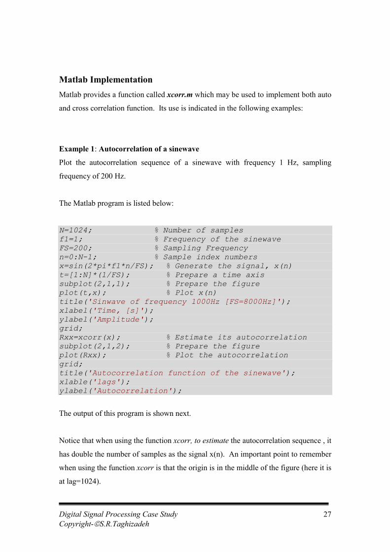
Matlab ImplementationMatlab provides a function called xcorr.m which may be used to implement both auto

and cross correlation function. Its use is indicated in the following examples:

Example 1: Autocorrelation of a sinewave

Plot the autocorrelation sequence of a sinewave with frequency 1 Hz, sampling

frequency of 200 Hz.

The Matlab program is listed below:

N=1024; % Number of samplesf1=1; % Frequency of the sinewaveFS=200; % Sampling Frequencyn=0:N-1; % Sample index numbersx=sin(2*pi*f1*n/FS); % Generate the signal, x(n)t=[1:N]*(1/FS); % Prepare a time axis subplot(2,1,1); % Prepare the figureplot(t,x); % Plot x(n)title('Sinwave of frequency 1000Hz [FS=8000Hz]');xlabel('Time, [s]');ylabel('Amplitude');grid;Rxx=xcorr(x); % Estimate its autocorrelationsubplot(2,1,2); % Prepare the figureplot(Rxx); % Plot the autocorrelationgrid;title('Autocorrelation function of the sinewave');xlable('lags');ylabel('Autocorrelation');

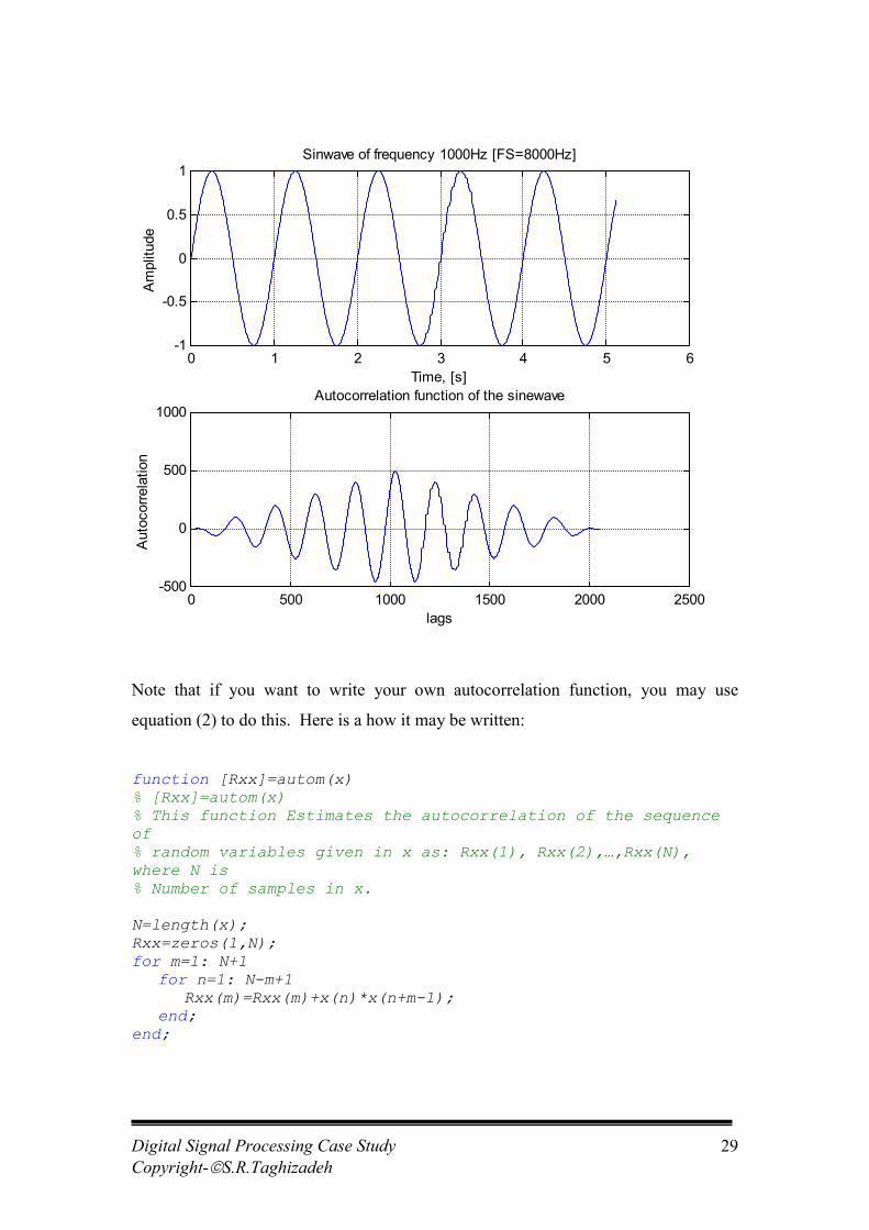
The output of this program is shown next.

Notice that when using the function xcorr, to estimate the autocorrelation sequence , it

has double the number of samples as the signal x(n). An important point to remember

when using the function xcorr is that the origin is in the middle of the figure (here it is

at lag=1024).


28


29

Note that if you want to write your own autocorrelation function, you may use

equation (2) to do this. Here is a how it may be written:

function [Rxx]=autom(x)% [Rxx]=autom(x)% This function Estimates the autocorrelation of the sequenceof % random variables given in x as: Rxx(1), Rxx(2),…,Rxx(N),where N is % Number of samples in x.

N=length(x);Rxx=zeros(1,N);for m=1: N+1

for n=1: N-m+1Rxx(m)=Rxx(m)+x(n)*x(n+m-1);

end;end;

0 1 2 3 4 5 6-1

-0.5

0

0.5

1Sinwave of frequency 1000Hz [FS=8000Hz]

Time, [s]

Am

plitu

de

0 500 1000 1500 2000 2500-500

0

500

1000Autocorrelation function of the sinewave

lags

Aut

ocor

rela

tion


30

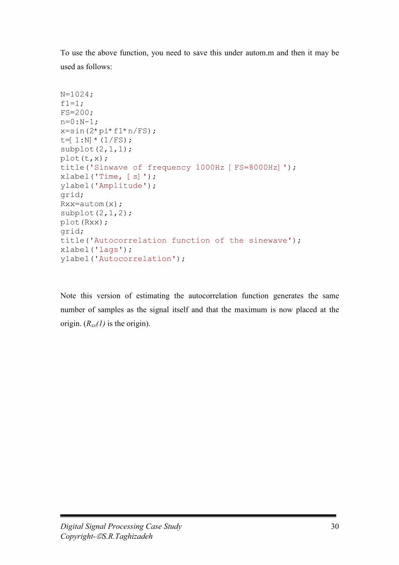
To use the above function, you need to save this under autom.m and then it may be

used as follows:

N=1024;f1=1;FS=200;n=0:N-1;x=sin(2*pi*f1*n/FS);t=[1:N]*(1/FS);subplot(2,1,1);plot(t,x);title('Sinwave of frequency 1000Hz [FS=8000Hz]');xlabel('Time, [s]');ylabel('Amplitude');grid;Rxx=autom(x);subplot(2,1,2);plot(Rxx);grid;title('Autocorrelation function of the sinewave');xlabel('lags');ylabel('Autocorrelation');

Note this version of estimating the autocorrelation function generates the same

number of samples as the signal itself and that the maximum is now placed at the

origin. (Rxx(1) is the origin).


31

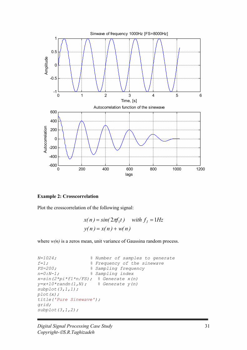
Example 2: Crosscorrelation

Plot the crosscorrelation of the following signal:

)n(w)n(x)n(yHzf with)tfsin()n(x 1

��

�� 12 1�

where w(n) is a zeros mean, unit variance of Gaussina random process.

N=1024; % Number of samples to generatef=1; % Frequency of the sinewaveFS=200; % Sampling frequencyn=0:N-1; % Sampling indexx=sin(2*pi*f1*n/FS); % Generate x(n)y=x+10*randn(1,N); % Generate y(n)subplot(3,1,1);plot(x);title('Pure Sinewave');grid;subplot(3,1,2);

0 1 2 3 4 5 6-1

-0.5

0

0.5

1Sinwave of frequency 1000Hz [FS=8000Hz]

Time, [s]

Am

plitu

de

0 200 400 600 800 1000 1200-600

-400

-200

0

200

400

600Autocorrelation function of the sinewave

lags

Aut

ocor

rela

tion


32

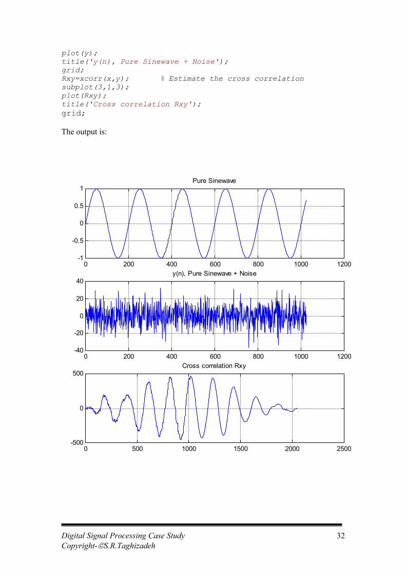
plot(y);title('y(n), Pure Sinewave + Noise');grid;Rxy=xcorr(x,y); % Estimate the cross correlationsubplot(3,1,3);plot(Rxy);title('Cross correlation Rxy');grid;

The output is:

0 200 400 600 800 1000 1200-1

-0.5

0

0.5

1Pure Sinewave

0 200 400 600 800 1000 1200-40

-20

0

20

40y(n), Pure Sinewave + Noise

0 500 1000 1500 2000 2500-500

0

500Cross correlation Rxy


Question [1]

From the results shown for example 2, what function cross correlation has performed.

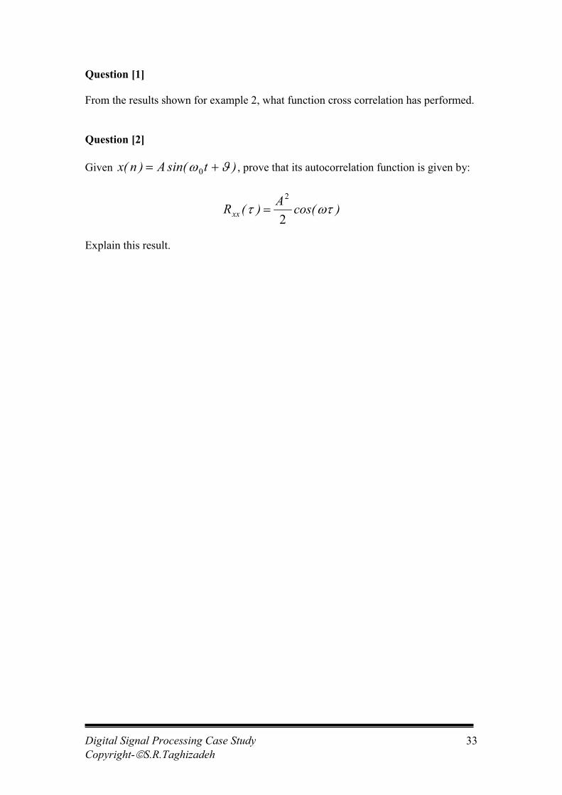
Question [2]

Given )tsin(A)n(x �� 0 , prove that its autocorrelation function is given by:

)cos(A)(Rxx ��

2

2

�

Explain this result.

33


34

Case Study

Time Delay EstimationProcessing Radar Returned Signal

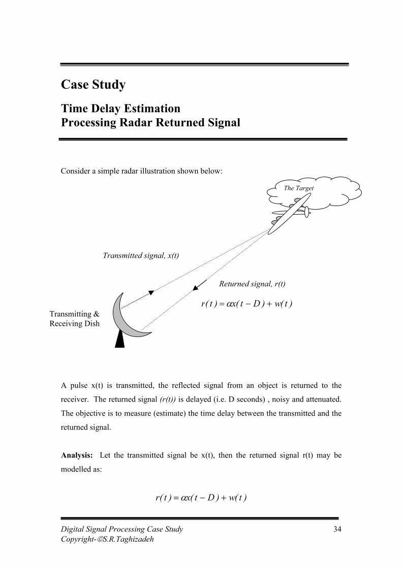
Consider a simple radar illustration shown below:

A pulse x(t) is transmitted, the reflected signal from an object is returned to the

receiver. The returned signal (r(t)) is delayed (i.e. D seconds) , noisy and attenuated.

The objective is to measure (estimate) the time delay between the transmitted and the

returned signal.

Analysis: Let the transmitted signal be x(t), then the returned signal r(t) may be

modelled as:

)t(w)Dt(x)t(r ��

The Target

Returned signal, r(t)

Transmitted signal, x(t)


Transmitting &Receiving Dish


35

where: w(t) is assumed to be the additive noise during the transmission.

� is the attenuation factor (<1).

D is the delay which is the time taken for the signal to travel from the

transmitter to the target and back to the receiver.

A common method of estimating the time delay D is to compute the cross-correlation

function of the received signal with the transmitted signal x(t). i.e.

� �

� ��

� �

)(R)D(R)(R

Hence)w(t)x(t)D)x(t-x(tE

)t(xw(t)D)-x(tE )t(x)t(rE)(R

wxxxrx

rx

��

��

��

��

��

��

��

��

(6)

Note, ‘E’ is the expectation operator.

Therefore, the cross correlation )(Rrx � is equal to the sum of the scaled

autocorrelation function of the transmitted signal (i.e. )(Rxx �� ) and the cross

correlation function between x(t) and the contaminated noise signal w(t). If we now

assume that the noise signal w(t) and the transmitted signal x(t) are uncorrelated then,

0�)(Rwx �

This is also stated in table 1.2 under the property number [6].

Hence the cross-correlation function between the transmitted signal and the received

signal may be written as:

)D(R)(R xxrx �� (7)


36

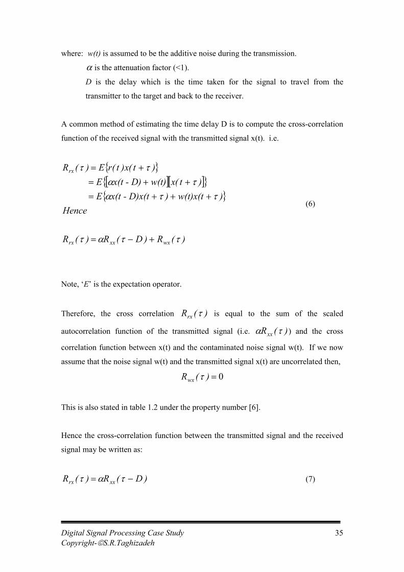
Therefore if we plot )(Rrx � , it will only have one peak value that will occur at

D�� . A typical plot of )(Rrx � is shown below:

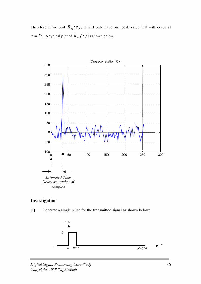
Investigation

[1] Generate a single pulse for the transmitted signal as shown below:

0 50 100 150 200 250 300-100

-50

0

50

100

150

200

250

300

350Crosscorrelation Rrx

Estimated TimeDelay as number of

samples

x(n)

0 N=256

5

n=4n


37

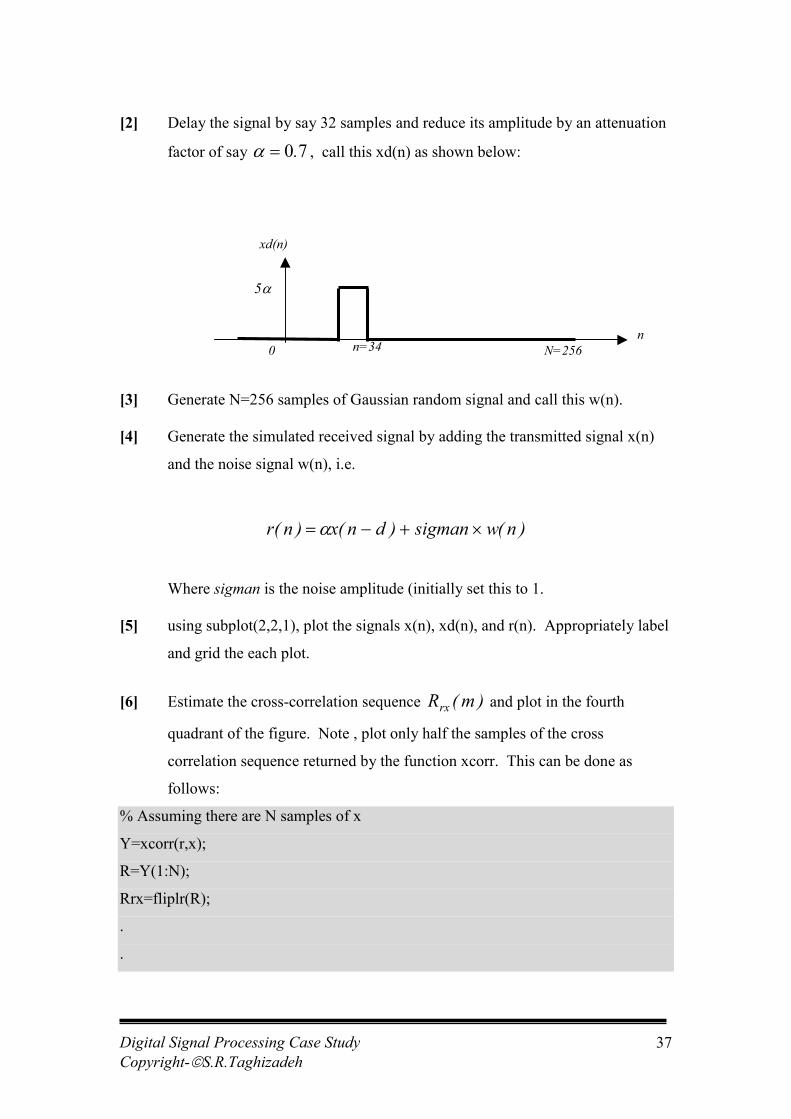
[2] Delay the signal by say 32 samples and reduce its amplitude by an attenuation

factor of say 70.�� , call this xd(n) as shown below:

[3] Generate N=256 samples of Gaussian random signal and call this w(n).

[4] Generate the simulated received signal by adding the transmitted signal x(n)

and the noise signal w(n), i.e.

)n(wsigman)dn(x)n(r ��

Where sigman is the noise amplitude (initially set this to 1.

[5] using subplot(2,2,1), plot the signals x(n), xd(n), and r(n). Appropriately label

and grid the each plot.

[6] Estimate the cross-correlation sequence )m(Rrx and plot in the fourth

quadrant of the figure. Note , plot only half the samples of the cross

correlation sequence returned by the function xcorr. This can be done as

follows:

% Assuming there are N samples of x

Y=xcorr(r,x);

R=Y(1:N);

Rrx=fliplr(R);

.

.

xd(n)

0 N=256

5�

n=34n


38

[7] From the plot estimate the delay. Does it agree with the theoretical delay

value?

[8] Repeat the simulation for some values of � , sigman, and N?

[9] Comment on your findings?

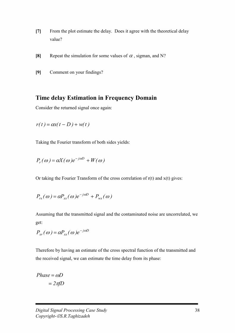
Time delay Estimation in Frequency DomainConsider the returned signal once again:


Taking the Fourier transform of both sides yields:

)(We)(X)(P Djr ��

�

��

Or taking the Fourier Transform of the cross correlation of r(t) and x(t) gives:

)(Pe)(P)(P wxDj

xxrx ��

��

Assuming that the transmitted signal and the contaminated noise are uncorrelated, we

get:Dj

xxxr e)(P)(P �

��

�

Therefore by having an estimate of the cross spectral function of the transmitted and

the received signal, we can estimate the time delay from its phase:

fD2 DPhase

�

�

�

�


39

Hence by taking the slope of the phase (i.e. Phase)f(d

d), we have the slope of the

phase which may be written as:

�

�

2

2

SlopeD

Or

DSlope

�

�

Here is how you may estimate the cross spectrum between the transmitted signal and

the received signal and to obtain the phase plot.

% Estimation of time delay using the phase of the CrossSpectrumPrx=csd(x,r); % Estimate the Cross Spectrumpha=angle(Prx); % Get the phasephase=unwrap(pha); % Unwrap the phaseplot(phase); % Plot the phase

InvestigationGenerate N=256 samples of a sinusoidal signal of amplitude 1 volts, frequency,

1f =1Hz. Use a sampling frequency, sF =200Hz, and call this signal the transmitted

signal, x(t).(i.e. )tfsin()t(x 12�� )

Generate a received signal r(t) as follows:

r(t) is also a sinusoidal of the same frequency whose amplitude has been attenuated by

0.5 and delayed by 2.5 Seconds. Add white noise with zero mean and a variance of

0.01. (i.e. )t(w)).t(fsin(.)t(r �� 52250 1� )

Plot x(t) and y(t).


40

Estimate and plot:

� The spectrum of the transmitted signal and the received signal.

� The autocorrelation of x(t) and r(t).

� The cross correlation between x(t) and r(t).

From this plot estimate the delay time (Time where it peaks) and compare to the

theoretical value of 2.5s.

Estimate the attenuation factor using:

x(t) of ationAutocorrel the of value peak TheD at peak the of Value

)(R)D(R

xx

xr �

��

�

�

1

Compare this value to the theoretical value of 0.5.

� Repeat the experiment for the noise variance of 0, 0.1,0.4, and 0.8.

� Estimate the error in each case.

� The cross spectral density and phase between x(t) and r(t).

From the phase plot, estimate the slope of the plot in the following table:

N Slope

128

256

512

1024

What is the relationship between the time delay and the slope of the phase?

[Note: That yet another method of estimating the time delay is via a system

identification approach. This method is described in the appendix for those

interested.]


41

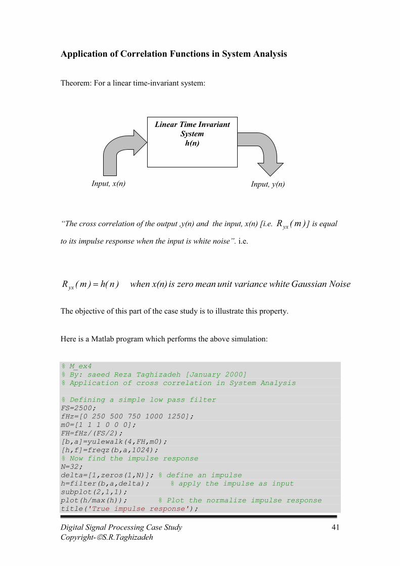
Application of Correlation Functions in System Analysis

Theorem: For a linear time-invariant system:

“The cross correlation of the output ,y(n) and the input, x(n) [i.e. )m(Ryx ] is equal

to its impulse response when the input is white noise”. i.e.

Noise Gaussian whitevariance unit mean zero is x(n) when)n(h)m(Ryx �

The objective of this part of the case study is to illustrate this property.

Here is a Matlab program which performs the above simulation:

% M_ex4% By: saeed Reza Taghizadeh [January 2000]% Application of cross correlation in System Analysis

% Defining a simple low pass filterFS=2500;fHz=[0 250 500 750 1000 1250];m0=[1 1 1 0 0 0];FH=fHz/(FS/2);[b,a]=yulewalk(4,FH,m0);[h,f]=freqz(b,a,1024);% Now find the impulse responseN=32;delta=[1,zeros(1,N)]; % define an impulseh=filter(b,a,delta); % apply the impulse as inputsubplot(2,1,1);plot(h/max(h)); % Plot the normalize impulse responsetitle('True impulse response');

Linear Time InvariantSystem

h(n)

Input, x(n) Input, y(n)


42

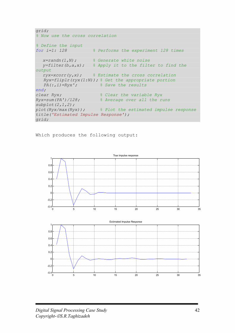
grid;% Now use the cross correlation

% Define the inputfor i=1: 128 % Performs the experiment 128 times

x=randn(1,N); % Generate white noisey=filter(b,a,x); % Apply it to the filter to find the

outputryx=xcorr(y,x); % Estimate the cross correlation

Ryx=fliplr(ryx(1:N)); % Get the appropriate portion PA(:,i)=Ryx'; % Save the resultsend;clear Ryx; % Clear the variable RyxRyx=sum(PA')/128; % Average over all the runssubplot(2,1,2);plot(Ryx/max(Ryx)); % Plot the estimated impulse responsetitle('Estimated Impulse Response');grid;

Which produces the following output:

0 5 10 15 20 25 30 35-0.4

-0.2

0

0.2

0.4

0.6

0.8

1True impulse response

0 5 10 15 20 25 30 35-0.4

-0.2

0

0.2

0.4

0.6

0.8

1Estimated Impulse Response


43

Note that the cross correlation technique produces a good estimate of the impulse

response of the system.

Note also that since the input is white noise and being random, the experiment will

not be valid for simply one run, hence as shown in the program, the simulation is

carried out for 128 times and the final result is the average of the all the runs. When

simulating with random processes, you must perform a simulation over a number of

runs and average the results for the final outcome.

InvestigationA digital filter is described by the following transfer function:

One of the most simplest and yet effective digital filters are ‘avergers’. This is a

system which computes the average of previous q-samples of its input. For example a

5-point averager is defined as:

� �)n(x)n(x)n(x)n(x)n(x)n(y 432151

��

For this system:

� Draw the filter structure.

� Use Matlab to plot its frequency response. Use:

a=1;

b=[1/5, 1/5, 1/5, 1/5, 1/5];

[h,f]=freqz(b,a,256);

H=abs(h);

f=f/(2*pi);

plot(f,H);

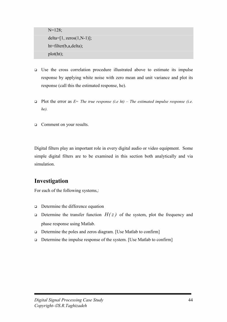
� Plot its impulse response. Use:


44

N=128;

delta=[1, zeros(1,N-1)];

ht=filter(b,a,delta);

plot(ht);

� Use the cross correlation procedure illustrated above to estimate its impulse

response by applying white noise with zero mean and unit variance and plot its

response (call this the estimated response, he).

� Plot the error as E= The true response (i.e ht) – The estimated impulse response (i.e.

he).

� Comment on your results.

Digital filters play an important role in every digital audio or video equipment. Some

simple digital filters are to be examined in this section both analytically and via

simulation.

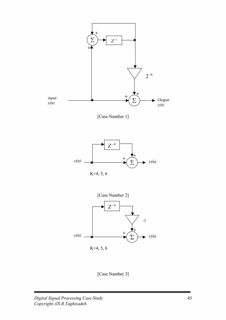
InvestigationFor each of the following systems,:

� Determine the difference equation

� Determine the transfer function )z(H of the system, plot the frequency and

phase response using Matlab.

� Determine the poles and zeros diagram. [Use Matlab to confirm]

� Determine the impulse response of the system. [Use Matlab to confirm]


45

[Case Number 1]

[Case Number 2]

[Case Number 3]

1�Z�

+

+

�

++

62�

Outputy(n)

inputx(n)

�

++

kZ �

y(n)x(n)

K=4, 5, 6

�

++

kZ �

y(n)x(n)

K=4, 5, 6

-1


46

Appendix ASystem Identification approach in Time Delay estimation

Here, we assume that the transmitted signal r(t) is the output of a linear time-invariant

system whose input is the transmitted signal x(t). Another word, we model a system

whose transfer function characteristic processes x(t) in a way as to produce the

transmitted signal r(t) in its output. Once this is done, the information concerning the

estimation of delay (i.e. D) may be extracted from its transfer function. Here is the

mathematical analysis of the above procedure.

From the theory of cross correlation, we have:

)(P).(H)(P xxxr ��

Which states that “The cross spectrum of the input-output, )(Pxr � is equal to the

transfer function )(H � times the power spectrum of the input signal, )(Pxx � .”

We therefore have:

)(P)(P

)(Hxx

xr

�

�

� �

Having obtained the transfer function of the model, the followings may be obtained:

Linear Time InvariantSystemH(�)

Input, x(t) Input, r(t)


47

)(P)(H)()(H

xr ��

��

��

�

The time delay (i.e.D) may be obtained from the slope of the phase angle )(�� as

before.

.


48

autocorrelation and crosscorrelation in matlab

Documents