automated buildin monitoring g using a wireles sensos ... · 3.4.4 databas 11e 5 3.4.5 use...
TRANSCRIPT

Automated Building Monitoring using a Wireless Sensor Network
Vahid Safar-Nourollah
A Thesis in
The Department of
Computer Science and Software Engineering
Presented in Partial Fulfillment of the Requirements For the Degree of Master of Computer Science
Concordia University Montreal, Quebec, Canada
March 2009
© Vahid Safar-Nourollah, 2009

1*1 Library and Archives Canada
Published Heritage Branch
Bibliothdque et Archives Canada
Direction du Patrimoine de l'6dition
395 Wellington Street Ottawa ON K1A 0N4 Canada
395, rue Wellington Ottawa ON K1A 0N4 Canada
Your file Votre r4f6rence ISBN: 978-0-494-63338-0 Our file Notre r6f6rence ISBN: 978-0-494-63338-0
NOTICE: AVIS:
The author has granted a non-exclusive license allowing Library and Archives Canada to reproduce, publish, archive, preserve, conserve, communicate to the public by telecommunication or on the Internet, loan, distribute and sell theses worldwide, for commercial or non-commercial purposes, in microform, paper, electronic and/or any other formats.
L'auteur a accorde une licence non exclusive permettant a la Bibliotheque et Archives Canada de reproduire, publier, archiver, sauvegarder, conserver, transmettre au public par telecommunication ou par I'lnternet, preter, distribuer et vendre des theses partout dans le monde, a des fins commerciales ou autres, sur support microforme, papier, electronique et/ou autres formats.
The author retains copyright ownership and moral rights in this thesis. Neither the thesis nor substantial extracts from it may be printed or otherwise reproduced without the author's permission.
L'auteur conserve la propriete du droit d'auteur et des droits moraux qui protege cette these. Ni la these ni des extraits substantiels de celle-ci ne doivent etre imprimes ou autrement reproduits sans son autorisation.
In compliance with the Canadian Privacy Act some supporting forms may have been removed from this thesis.
While these forms may be included in the document page count, their removal does not represent any loss of content from the thesis.
Conformement a la loi canadienne sur la protection de la vie privee, quelques formulaires secondaires ont ete enleves de cette these.
Bien que ces formulaires aient inclus dans la pagination, il n'y aura aucun contenu manquant.
Canada

Concordia University School of Graduate Studies
This is to certify that the thesis prepared
By: Entitled:
Vahid Safar-Nourollah Automated Building Monitoring using a Wireless Sensor Network
and submitted in partial fulfillment of the requirements for the degree of
Master of Computer Science
complies with the regulations of this University and meets the accepted standards with respect to originality and quality.
Signed by the final examining committee:
Dr. H. Harutyunyan
Dr. J. Opatrny
Dr. J. W. Atwood
Chair
Examiner
Examiner
Dr. Lata Narayanan Supervisor
Approved by Chair of Department or Graduate Program Director
20 Dr. Robin A.L. Drew, Dean Faculty of Engineering and Computer Science

Abstract Automated Building Monitoring using a Wireless Sensor Network
Vahid Safar-Nourollah
Building monitoring is one of the challenging issues in building construction,
due to its high cost and the time consuming procedure for implementation and
maintenance. It is also a critical issue that directly affects building security, safety,
and management, energy saving, and tenants' convenience. Wireless sensor net-
working is a new networking technology that holds great promise for monitoring,
evaluation and management of buildings. However, sufficient work has not been
done in the application part of wireless sensor networks for building monitoring.
In this thesis, we show how advanced wireless sensor technology can be used by
building managers to monitor climate conditions, brightness level, lamp status
and room occupancy in buildings as well as by the wireless sensor network ad-
ministrator to monitor the nodes' connectivity and conditions in the network. We
conceive of the building monitoring application as being divided into three main
parts. First, wireless sensor hardware is programmed to process signals from sen-
sors and transmit the data in a suitable format to a gateway/server application
using multi-hop routing. The second task involves the forwarding of the signals
sent by the wireless sensor nodes to the end user application by the gateway/server
application. The gateway/server also archives the sensor data in a database for
iii

further retrieval and analysis. The third part consists of an end user application
for processing the sensor data sent by the wireless sensor nodes and then forwarded
by the gate way/server. The end user application visualizes the network topology,
network connectivity graph and real time information of individual motes. In addi-
tion, this application provides the real time analysis of the data and functionalities
for search and observation. Finally, the end user application allows users to an-
alyze the rooms and network conditions by mining the database using different
parameters such as the type of data and the time of data acquisition. The system
and related analysis were applied on a real case study — the eighth and ninth
floors of the Engineering and Visual Arts building of Concordia University.
iv

Acknowledgments
I would like to express my special gratitude to my supervisor, Dr. Lata Narayanan,
whose support and guidance contributed to my graduate work and experience. A
sincere thank you to Mr. Mohsen Eftekhari, a member of Network labs group, for
his help in system deployment and his valuable comments on this work.
I owe my loving thanks to my wife, Elaheh Safari, for her help, support, en-
couragement and understanding. I warmly thank my family, who has encouraged
me during my studies.
This work is partially funded by the Natural Sciences and Engineering Research
Council of Canada (NSERC).
v

Contents
List of Figures x
List of Tables xvii
1 Introduction 1
1.1 Motivation 4
1.2 Problem definition 8
1.2.1 End user application 8
1.2.2 Wireless sensor network 11
1.2.3 Gateway/server 13
1.3 Contributions 14
1.4 Organization of dissertation 16
2 Literature survey 17
2.1 Wireless sensor network applications 17
2.1.1 Areas 18
vi

2.1.2 Classification of sensor network applications 26
2.1.3 Design problems for building monitoring applications . . . . 29
2.2 Wireless sensor network platforms 32
2.2.1 Processing unit 32
2.2.2 Radio transceiver 34
2.2.3 Sensor 35
2.2.4 Selection criteria 36
2.3 Wireless sensor network routing algorithms 39
2.3.1 Flat routing 40
2.3.2 Hierarchical routing 49
2.3.3 Location based routing 51
2.3.4 Selection criteria 51
3 Automated Building Monitoring System 59
3.1 Technologies 60
3.1.1 NesC 60
3.1.2 TinyOS 61
3.1.3 Cygwin 64
3.1.4 J2SE 1.4 65
3.1.5 MySQL server 5.2 65
3.1.6 UML 66
3.2 System Architecture 66
vii

3.3 Wireless sensor network 68
3.3.1 Platform 68
3.3.2 Design 77
3.3.3 Sensing functions 81
3.3.4 Lamp status (room occupancy) 84
3.3.5 Routing algorithm 90
3.3.6 Synchronization 102
3.3.7 Sensornet protocol 107
3.4 Gateway/server I l l
3.4.1 Design and features I l l
3.4.2 Sink connection 114
3.4.3 Internet connection 114
3.4.4 Database 115
3.4.5 User interface 118
3.5 End user application 119
3.5.1 Design 119
3.5.2 Server connection 122
3.5.3 Message interpretation 123
3.5.4 Real time topology visualization 133
3.5.5 Messages and alerts central panel 140
3.5.6 Real time data and link quality charting 144
viii
3.5.7 Data query and analysis for building managing 149
3.5.8 Data query and analysis for network administrating 152
4 Data collection and analysis 156
4.1 System deployment 156
4.2 System analysis 161
4.2.1 System correctness 161
4.2.2 System robustness 162
4.2.3 Network reliability 162
4.2.4 Network lifetime 166
4.3 Data analysis 168
4.3.1 Lamp status (room occupancy) data analysis 168
4.3.2 Brightness data analysis 169
4.3.3 Temperature and humidity data analysis 172
4.4 Discussion 177
5 Conclusion and recommendations for future work 180
Bibliography 183
Appendices 197
A Installation guide 197
B End user application and gateway/server design 200
ix
List of Figures
1 Automated Building Monitoring system by wireless sensor network
architecture 67
2 Front and back side of Tmote Sky module 69
3 Channel comparisons between IEEE 802.11 and IEEE 802.15.4 . . . 72
4 Accuracy of Sensirion relative humidity and temperature sensors . . 73
5 Photo sensitivity of the light sensors on Tmote Sky 76
6 Short circuit current linearity 78
7 Graphical veiw of components relations of the motes application . . 80
8 Voltage-time graph of an AC power electrical signal 86
9 Changes of TSR and PAR raw readings when lamps are switched
on or off in the rooms without daylight 88
10 Changes of TSR and PAR raw readings when lamp is switched on
or off during variable cloudy day in period of one hour in the room
with daylight 89
x

11 Changes of TSR and PAR raw readings when the light in the room
is from Sun only 90
12 Changes of TSR and PAR raw readings when the light in the room
is from both Sun and the lamps 91
13 An example of selecting best route by the motes to the sink using
the MultiHop routing algorithm 94
14 Graphical view of components relation of MultiHop component . . . 97
15 Graphical view of components relation of NetSync component . . . 108
16 Graphical view of components relation of Sensornet component . . 110
17 Package diagram of the gateway/server 112
18 The database schema for bm database 115
19 Gateway/server user interface 118
20 Package diagram of the end user application 120
21 Server connection frame 123
22 The graphical user interface for showing the information of selected
mote 132
23 The graphical user interface for showing the information of all motes 134
24 The graphical user interface for finding the rooms with defined criteria 135
25 The graphical user interface for real time visualization of the net-
work topology 137
26 The graphical user interface for controlling the visualization panel . 138
xi

27 The Information that can be shown in the visualization panel for
the motes and their connectivity 141
28 The graphical user interface for displaying messages and alerts of
the system 143
29 The graphical user interface for charting the real time sensed data . 145
30 The graphical user interface for charting the link quality of the links 146
31 The graphical user interface for editing legend of real time data
charting 147
32 The graphical user interface for editing legend of real time link qual-
ity charting 148
33 The graphical user interface for querying database and analyzing
retrieved data by the users responsible for building managing . . . . 150
34 The graphical user interface for selecting motes (rooms) for data
query and analysis 153
35 The graphical user interface for querying database and analyzing
retrieved data by the users responsible for the network administrating 154
36 Floor map 157
37 Tmote Sky mote (the 2$ coin is placed alongside to give an idea of
the actual size of the mote) 158
38 The placement of the mote over the lamps frame of room 8.161 . . . 160
xii
39 Ratio of successfully received and lost messages to total expected
messages for each mote in the network 164
40 One-hop neighbor motes distribution and average link quality of
mote 9101 in room 9.101 165
41 One-hop neighbor motes distribution and average link quality of
mote 8210 in room 8.210 166
42 Remained and used power source of all motes 167
43 Lamp status (room occupancy) statistics during the 50 days of test-
ing period 170
44 Minimum and maximum of the brightness in all rooms when the
lamps are on 171
45 Brightness level in room 8.101 on October 2nd from 8:24AM to
2:49PM. Note that lamp status was off during this period 172
46 Temperature, humidity and lamp status changes in room 8.165 dur-
ing one day of the testing period 174
47 Temperature, humidity and lamp status changes in room 8.173 dur-
ing one day of the testing period 175
48 Minimum, maximum and average of temperature in all rooms when
the ventilation and heating systems were on during the testing period 176
49 Distribution of the temperature values in room 8.165 when the ven-
tilation and heating systems were on during the testing period . . . 177
xiii

50 End user application 201
51 Package com.concordia.bm 202
52 Class com.concordia.bm.BM 203
53 Class com.concordia.bm.DataCalculation 204
54 Class com.concordia.bm.DateUtils 205
55 Class com.concordia.bm.FileHandler 206
56 Class com.concordia.bm.Renderer 207
57 Class com.concordia.bm.Updater 208
58 Package com.concordia.bm.chart 209
59 Class com.concordia.bm.chart.Channel 210
60 Class com.concordia.bm.chart.ControlPanel 211
61 Class com.concordia.bm.chart.GraphPanel 212
62 Class com.concordia.bm.chart.Oscilloscope 213
63 Class com.concordia.bm.chart.ScopeDriver 214
64 Package com.concordia.bm.client 215
65 Class com.concordia.bm.client.TCPClient 216
66 Class com.concordia.bm.client.TCPConnectionGUI 217
67 Class com.concordia.bm.client.TCPInterface 218
68 Class com.concordia.bm.client.VirtualMessageCreator 219
69 Package com.concordia.bm.db 220
70 Class com.concordia.bm.db.DBConnection 221
xiv
71 Class com.concordia.bm.db.DBLinkTable 222
72 Class com.concordia.bm.db.DBReadingTable 223
73 Class com.concordia.bm.db.DBUpdateQuery 224
74 Package com.concordia.bm.gui 225
75 Class com.concordia.bm.gui.FrameFindRoom 226
76 Class com.concordia.bm.gui.FrameMain . 227
77 Class com.concordia.bm.gui.FrameMessagesAlerts 228
78 Class com.concordia.bm.gui.FrameSelectRooms 229
79 Class com.concordia.bm.gui.FrameTCPConnection 230
80 Class com.concordia.bm.gui.FrameTopologyTable 231
81 Class com.concordia.bm.gui.PanelBuildingManagerQ 232
82 Class com.concordia.bm.gui.PanelNetworkAdminQA 233
83 Class com.concordia.bm.gui.TablRealTimeTopology 234
84 Class com.concordia.bm.gui.Tab2RealTimeDataChartting 235
85 Class com.concordia.bm.gui.Tab3RealTimeLinkQualityChartting . . 236
86 Class com.concordia.bm.gui.Tab4BuildingManagingQA 237
87 Class com.concordia.bm.gui.Tab5NetworAdministratingQA 238
88 Class com.concordia.bm.gui.Tab6CommandingNetwork 239
89 Package com.concordia.bm.motes 240
90 Class com.concordia.bm.motes.BMapplMsg 241
91 Class com.concordia.bm.motes.MultiHopMsg 242
xv

92 Package com.concordia.bm.topology 243
93 Class com.concordia.bm.topology.GraphIO 244
94 Class com.concordia.bm.topology.LinkData 245
95 Class com.concordia.bm.topology.MoteGraph 246
96 Class com.concordia.bm.topology.NodeData 247
97 Class com.concordia.bm.topology.NodeTips 248
98 Class com.concordia.bm.topology.Topology 249
99 Class com.concordia.bm.topology.TopologyDriver 250
100 gateway/server 251
101 Package com.concordia.bm.motes 252
102 Class com.concordia.bm.motes.BMapplMsg 253
103 Class com.concordia.bm.motes.MultiHopMsg 254
104 Class com.concordia.bm.motes.UartDetectConsts 255
105 Class com.concordia.bm.motes.UartDetectMsg 256
106 Package com.concordia.motesbridge 257
107 Class com.concordia.motesbridge.ClientsHandler 258
108 Class com.concordia.motesbridge.MotesBridge 259
109 Class com.concordia.motesbridge.MotesInterface 260
110 Class com.concordia.motesbridge.UartDetect 261
xvi

List of Tables
1 The evolution of the UCB mote platforms [62] 38
2 Power consumption of Tmote Sky 70
3 Sensirion relative humidity and temperature performance specifica-
tions 75
4 Equivalence of real world examples to different lux values 77
5 Predefined thresholds of sensor readings for alerting the end user . . 84
6 Data messages structure in MultiHop routing algorithm 100
7 BMappl message structure in MultiHop routing algorithm 101
8 Route update beacons structure in MultiHop routing algorithm . . . 101
9 Considered factors for calculating required duty cycle for the wire-
less sensor network 103
10 Lifetime of the motes with different duty cycles 106
xvii

Chapter 1
Introduction
A Wireless Sensor Network (WSN) consists of spatially distributed autonomous de-
vices (motes) using sensors in order to cooperatively sense physical or environmen-
tal conditions, such as temperature, vibration, pressure or pollutants at different
locations. The motes send raw or processed data using their radio transceiver to
the base (sink) node(s) using multi-hop communications [29, 67]. The base nodes
are one or more distinguished components of the wireless sensor network with
more computational, energy and communication resources. They act as a gate-
way between sensor nodes and the end user. Sensor nodes can be considered as
small computers, extremely basic in terms of their interfaces and their components.
They consist of a processing unit with limited computational power and limited
memory, sensors (including specific conditioning circuitry), a communication de-
vice (usually radio transceivers or alternatively optical), and a power source mostly
1

in the form of battery. Other possible inclusions are energy harvesting modules,
and secondary communication devices (e.g., USB).
The basic premise of a wireless sensor network is to perform networked sensing
using a large number of relatively unsophisticated sensors, instead of the conven-
tional approach of deploying a few expensive and sophisticated sensing modules.
The potential advantage of networked sensing over the conventional approach, can
be summarized as greater coverage, accuracy and reliability at a possibly lower
cost. Some of the early works on wireless sensor network [14, 18, 19] motivate and
discuss these benefits in detail. In other words, wireless sensor networks include
the ability to withstand harsh environmental conditions, ability to cope with node
failures, have dynamic network topology, be able to have large scale of deployment
with unattended operation, ease of installation, time awareness for coordination
with other nodes and self-diagnosis reliability. However, these networks have their
own unique constraints and challenges, which include limited power, limited net-
work communication bandwidth and limited memory [94],
The development of wireless sensor networks was originally motivated by mili-
tary applications such as battlefield surveillance. However, wireless sensor networks
are now under development for further usage in many civilian application areas,
including environment and habitat monitoring, health care applications, home au-
tomation, and traffic control [28, 67], In a typical application, a wireless sensor
network is scattered in a region to collect data through its sensor nodes.
2

Area monitoring is one of the common applications of wireless sensor networks.
In area monitoring, the wireless sensor network is deployed over a region where
some specific phenomena or several area conditions should be monitored. When
the defined event or the real time condition of the area (heat, pressure, sound,
light, electro-magnetic field, vibration, etc.) is detected by the sensors, the raw or
processed data is reported to one of the base stations in order to take appropriate
action (e.g., send a message on the Internet or to a satellite). Depending on the
exact application, different functions require different data-propagation strategies,
based on the needs for real-time response, redundancy of the data, security, etc.
Building monitoring is one of the challenging issues for building constructors
in terms of its high cost and time consuming procedure for implementation and
maintenance. Building monitoring is also one of the most critical issues in building
operation, in that directly affects building security, safety, energy saving, manage-
ment and tenants' convenience. Beside the obvious discomfort associated with
variation in internal environmental conditions for building tenants, there are real
economic costs as reflected in lost productivity and wasted energy due to poorly
moderated building climates. Wireless sensor networking is a new networking
technology that holds great promises for evaluation and management of building
climates [47], In addition, the existing wireless sensor network applications are not
sufficient to satisfy the above mentioned requirements for building monitoring [6].
Thus, we need to develop and deploy a wireless sensor network system that is able
3

to provide security, safety, energy saving, management and tenants' convenience
in buildings.
This thesis aims to introduce a new wireless sensor network system, which is
able to monitor building climate and room occupancy, to be used instead of ex-
isting building monitoring systems while providing better building safety, energy
saving, management and tenants' convenience with lower cost and time for imple-
mentation and maintenance. In this thesis, we have investigated the possibility of
how a wireless sensor network can meet such needs and bring the new generation
of network technology in this area of industry. The research in this study is con-
ducted through real wireless sensor network modeling and testing of the building
monitoring system application for monitoring, visualization and analysis of the
climate conditions and room occupancy.
1.1 Motivation
Building monitoring systems exist in most of the commercial buildings with the
first duty of providing convenience and safety. However, implementation and main-
tenance of wired systems are time consuming, error-prone and costly (e.g., for ex-
isting construction: 2.2$ per linear foot and for new construction: 0.67$ per linear
foot [6]). Another issue is when some crisis happens for a building, such as earth-
quake or fire. Since the damage to the construction make the backbone system
fail, the whole system stops operating.
4

The new technology of wireless sensor network has brought a new level of
building monitoring systems by saving the cost and time of implementation and
maintenance, providing more safety and robustness and making these systems
more stable in hazardous circumstances [47, 57]. The stability of these systems
in hazardous circumstances is due to the nature of wireless sensor network, in
that each mote in the network is independent of the other motes, they are battery
powered, small in size with attached sensors. Also, two other important features
that make these systems stable are communication by radio and formation of a
mesh network.
In a mesh network, each mote finds the best way through its neighbor motes
to the sink. In case of failure of intermediate mote(s) to the sink, data will be
redirected by other routes to the sink. Thus, in this situation, the whole network
can always operate without any failure related to the lack of functionality of some
motes. Moreover, the system is capable of adjusting to any building structure. It is
important to mention that with a wired backbone system, we cannot apply major
modifications or renovations to the system without costly and time consuming
procedures. However, with a wireless sensor network, both the cost and the time
to accommodate various modifications such as renew, add, remove, rearrange and
replace sensor nodes, is lower. For instance, in case of upgrading or renewing an
old building monitoring system of a hospital, the following tasks should be done:
shutting down all systems, changing the cables and wiring by going through the
5

walls and taking out the old sensors, replacing them with new ones. However, for
renewal of such systems by wireless sensor network, all these mentioned tasks can
be done by placing the motes in the needed places.
Nowadays, the average cost of each mote is about 100 CAD but it is predicted
by Intel and Cnet companies that each of them will cost few cents in the near
future [37, 57]. In addition, source code of the motes is developed in open source
programming language and operating system such as NesC and TinyOS [56, 60]. As
a result, wireless sensor applications can have the following advantages: availability
of the source code with the right to modify it by enabling the unlimited tuning
and improvement of a software product and the right to redistribute modifications
and improvements to the code for more reusability.
We summarize below the advantages of wireless sensor networks for building
monitoring applications:
• Simple, more flexible system design
• Faster and easier installations
• Smoother and less costly migration staged to accommodate budgets and
schedules
• More stability in hazardous circumstances
• Less cost and fewer constraints associated with maintenance
• Open source, more applicable to modification and improvement
6

During the last decade, there have been several research projects that have
led to some improvements in different areas (subfields) of wireless sensor networks
such as routing algorithms, MAC layer protocols, localization algorithms, data
gathering, hardware modules, radio transceivers etc. However, there has not been
enough focus on the application layer of this technology in building monitoring.
Despite the importance of wireless sensor networks in building monitoring [47],
the only major work in this field so far was done by Siemens [77] and UC Berke-
ley [87, 86, 21]. Teams at UC Berkeley have addressed mobile agents' localization
in the building for find-and-rescue missions, controlling indoor temperature by air-
flow measurement and controlling systems for producing temperature gradients
indoors to study energy implications of using sensor network. Siemens, which is
working in the building monitoring field more than any other research group, has
recently focused on using wireless sensor network to monitor the temperature of
the building only. More related work will be discussed in detail in Chapter 2.
As a summary, we can conclude that sufficient work has not been done in
the application part of wireless sensor network for building monitoring, despite
the promise of providing security, safety, accuracy, expandability and flexibility in
building monitoring.
7
1.2 Problem definition
The objectives of this thesis are to demonstrate the feasibility of implementing
a building monitoring system using a wireless sensor network, to understand the
involved challenges and to understand the extent and limitation of information
that can be obtained with such an approach.
A building monitoring system using a wireless sensor network clearly consists
of at least three parts — the end user application, the sensor network, and the
gateway/server to enable communication between the two. Each of the three needs
to perform a different set of functions. The requirements and specifications for
these three parts are described in the remainder of this section.
1.2.1 End user application
The end user application should satisfy different needs from two main categories
of building monitoring system users and beneficiaries: network administrator and
building manager. For this purpose, the application should have different features
as follows:
Visualization The network administrator should be able to see the connectivity
graph of the wireless sensor network, the whole network overview and status, real
time status of each mote (current power, remaining life time), real time status
of each mote's connectivity (current parent and two alternative parents), floor
8

plan of building with indication of location of each mote, total number of received
messages and lost messages of each mote, etc. However, the building manager,
would be interested in having the real time status of each room's climate such as
temperature and humidity, brightness and room occupancy.
Alerting For safety reasons, almost all users would like to be alerted in case
of any sudden change in the climate conditions of the building such as a sudden
temperature drop or rise. The process of alerting can be performed by informing
building manager first and then getting delegated to other users.
System overview and search The network administrator and building man-
ager should have an observation of the system overview based on real time data
received from the motes. In addition, they would be interested in having the ability
to search over the overview for all motes or rooms with some specific criteria. They
may be interested in finding rooms based on occupancy for different purposes such
as finding conference rooms which are empty or figuring out if a person is in room.
Real t ime charting The network administrator would be interested in the
charting of real time mote's status and network connectivity over time to en-
sure about the network functionality. However, the building manager would like
to have the overview of rooms climate conditions, brightness and room occupancy
over the time.
9

Analysis The network administrator is concerned about the analysis of the data
to evaluate the functionality of the network over time in order to inspect and fix
different problems such as high ratio of messages lost, low connectivity, high power
drop, etc., in individual or set of motes. Also the building manager is interested in
studying the climate in rooms over time in order to inspect and evaluate building
equipment functionality such as heating and ventilation systems. He would be
concerned about the analysis of the occupancy statistics of various rooms to assess
the proper usage of the building spaces over time. The building manager would
also be interested in studying the lamp status of rooms in different periods of
time to explore the proper usage of energy. Finally, both network administrator
and building manager are interested in having the ability to query the database
to extract all distinct dates and times in which the temperature, humidity or
brightness of different rooms have been requested.
Remote connection The users need to connect to the gateway/server remotely
from their offices. Therefore, in order to receive messages from the wireless sensor
network, the end user application should connect to the gateway/server over the
Internet. The connection has to be reliable and connection-based. The end user
application should also be able to extract the messages from the packets and queue
them for interpretation.
10

Message interpretation In the end user application, the user wants to have
the sensor readings to be categorized and understandable in metric units. Each
message received from the motes is a set of bytes that consists of different types of
data, which includes sensor readings, network connectivity status, mote's current
power, etc., in specific formats. The end user application has to distinguish all
distinct data from each message and calculate them in metric units. The data
extracted from the messages should be interpreted for different purposes such as
visualization, real time scaling, alerting, analysis, etc.
1.2.2 Wireless sensor network
The wireless sensor network should provide the necessary data for the end user
application to fulfill its requirements. In addition, the classification of the system
that we would plan to design is data gathering and reporting (discussed in detail
in Section 2.1.2). For the wireless sensor network, specific requirements should be
met as follows:
Quality of service The system should be reliable and robust, implying that the
motes should deliver the data to the end user with the most ratio of success (the
least ratio of lost messages) accurately. In addition, data should be delivered real
time (within a certain period of time from the moment it is sensed), otherwise the
data will be useless, since the sensed data in our application is critical toward the
safety of building tenants in cases such as sudden temperature drop or rise.
11

Multi-hop communication Our wireless sensor network needs to have mesh
network formation. Data have to be successfully sent to the base station from the
farthest motes in the sensor network over the multi-hop communication.
Lifetime of the network Also, this wireless sensor network should last long,
meaning that the motes that are battery powered and have limited energy source
have to be able to minimize the usage of their radio transceiver, beside having
minimum in mote data processing. For addressing the mentioned purpose (energy
conservation), the two following factors should be considered: first, synchronization
between motes to use the minimum necessary duty cycle of radio transceiver and
second, using power-saving algorithms for the radio and balancing the trade off
between communication versus computation. While considering the energy saving
issue, the system should still remain reliable and robust.
Sensing function Beside monitoring the building climate and brightness level
of the rooms, we are interested in monitoring the room occupancy, which is the
interest of many building monitoring systems. We would like to calculate the room
occupancy based on the readings of light sensors, since it avoids the use of external
sensors such as motion detectors. This way, we provide more energy conservation,
less and cheaper hardware usage and faster hardware installation.
Network monitoring function Finally, the system should provide information
about the status of the network connectivity and mote power. This information
12

can be used by the network administrator in order to have a detailed view of the
network.
1.2.3 Gateway/server
We need a gateway/server between wireless sensor network and end user applica-
tion. The gateway/server needs to run over a workstation connected to the sink
of the wireless sensor network and the Internet at the same time. In addition, the
mote data need to be archived in the database as well.
Sink connection The gateway should communicate in a synchronized way to the
sink through a port (usually USB) that connects the sink to the workstation. The
gateway and sink connection has to be implemented based on the sink hardware
and the type of used port. The implementation should be in such a way that
makes them synchronized and let the gateway recognize the data baud rate (data
transition speed) in order to distinguish distinct messages.
Internet connection It has to serve as a server for listening to any client and
forward the messages from sink to the client over the Internet. The gateway to
client connection has to be reliable and connection-based over the Internet.
Archiving The users need to have the data to be saved for later access and
analysis. Therefore, all data that is received from the motes is required to be
stored for further retrieval and analysis. The performance issue arises due to large
13

scale and short time interval of the received data. In order to address this issue, we
need to use a relational database management system to control the performance.
In addition to the above mentioned functional requirements of the end user ap-
plication, wireless sensor network and gateway, some non-functional requirements
should be considered to improve the quality of the system. These requirements
can include evolution and quality attributes such as reusability, extensibility and
scalability.
1.3 Contributions
In this thesis, we have proposed a system architecture for automated building mon-
itoring systems using a wireless sensor network for monitoring climate, brightness
and lamp status of the rooms in a building. We have implemented this system
which includes three sub systems, wireless sensor network, gateway/server, and
end user application.
The wireless sensor network reports the collected data for temperature, hu-
midity and brightness and the calculated lamp status (room occupancy) to the
sink while considering energy conservation by using a low power duty cycle. In
the wireless sensor network subsystem, we have deployed a simple new routing
algorithm which results from refining and combining two existing routing algo-
rithms. In addition, a new approach has been proposed for detecting lamp status
by using light sensors only. The lamp status of a room is an approximation of

the room occupancy. The routing algorithm was implemented to work on top of
the Sensornet Protocol [63] and in conjunction with the NetSync component [53]
for synchronization of the low power duty cycle. Necessary adjustments to the
NetSync component were also made.
The gateway/server forwards the received data from the sink to the end user
application that is connected to it. In addition, the gateway/server archives the
received data in a database for later retrieval and analysis.
The end user application visualizes the network connectivity. It provides tools
to view and search a mote's information. It also provides charts for analyzing the
information based on the received data for two categories of the users which are
building manager and network administrator. The application interprets the data
from the database in order to analyze the building climate, room occupancy and
brightness, and functionality of the heating, cooling and ventilation system of the
building.
The wireless sensor network has been developed in the NesC programming lan-
guage and Tinyos operating system. The gateway/server and end user application
have been designed in UML and implemented using an object oriented approach
in Java. The three main subsystems have been implemented and documented to
be reusable and extensible for future improvements.
We have implemented all of the components of all three subsystems for the
15

purpose of this thesis except two components in our wireless sensor network ap-
plication; NetSync for synchronization and SPC (Sensornet Protocol) for making
multiple network protocols work on the same MAC layer.
The system has been tested by applying it on a real case study and the collected
data has been analyzed and discussed in this dissertation.
1.4 Organization of dissertation
The rest of this dissertation is organized as follows: In Chapter 2, we provide some
necessary background on wireless sensor network applications, hardware platforms
and routing algorithms. The methodology of designing and developing the building
monitoring system using a wireless sensor network in order to address the problem
defined in Section 1.2 is explained in Chapter 3. In Chapter 4, we validate our
system by analyzing the system robustness and correctness along with network
reliability and life time. As well, we outline the analysis of collected data. Finally,
we list conclusions and recommendations for further work in Chapter 5.
16

Chapter 2
Literature survey
In this chapter, we provide the necessary background on wireless sensor network
applications, hardware platforms, algorithms and protocols that are within the
scope of this research.
2.1 Wireless sensor network applications
The range of potential applications that wireless sensor network are envisaged to
support is tremendous, encompassing military, civilian, environmental and com-
mercial areas [4], Wireless sensor network applications typically are involved in
monitoring, tracking, and controlling. These applications can be categorized by
their objectives, types of measured information, traffic characteristics, data de-
livery requirements and the way their design space is presented for deployment,
etc.
17

First, we describe different areas of major wireless sensor network applications.
Then, we explain different approaches that have been used for building monitoring
applications. We describe a classification of wireless sensor network applications
and finally, we explain the design issues involved in building monitoring applica-
tions.
2.1.1 Areas
The areas in which major wireless sensor network applications have been developed
or are under development and research can be categorized as follows [94]:
• Environmental monitoring
• Health care
• Industrial
• Security and surveillance
• Military
• Building monitoring and controlling
For each area, we explain how wireless sensor network can be used. In addition,
we mention major works that have been done so far in each case.
18

Environmental monitoring
In this area, sensors can be used to monitor conditions and movements of wild
animals or plants in wildlife habitats. They can also monitor air quality and
track environmental pollutants, wildfires, or other natural or man-made disasters.
Additionally, sensors can be used to monitor biological or chemical hazards to
provide early warnings for disasters such as earthquakes. In fact, in comparison
with other areas, environmental monitoring has the most developed applications
of sensor networks. Some examples of wireless sensor network applications in
this field are: an application to monitor volcanic eruptions with low-frequency
acoustic sensors developed by researchers at Harvard University and University of
North California [85]; a project with the aim of monitoring glacier behavior via
different sensors and linking them together into an intelligent web of resources [64];
a reactive, event driven network for environmental monitoring of soil moisture [13];
a deployed network consisting of 32 nodes on a small island off the coast of Maine,
streaming useful live data onto the web (Great Duck Island application) [81]; and
in the Mediterranean area, using wireless sensor network for monitoring wildfire
events [7],
Health care
Care for the elderly can greatly benefit from sensors that monitor vital signs of
patients and are remotely connected to doctors' offices. These applications can
19

include monitoring of human physiological data, tracking and monitoring of doctors
and patients inside an hospital, and drug administration in hospitals [71, 80].
Sensors instrumented in homes can also alert doctors when a patient's situation
becomes an emergency or he/she becomes physically incapacitated and requires
immediate medical attention. In addition, wireless sensor networks can be used to
optimize the health care system in hospitals. For instance, supporting the health
care workers in the night shift in which many patients have to be managed by
drastically reduced staff [17].
Industrial
Wireless sensors can be used to monitor manufacturing processes or the condi-
tions of industrial equipment. Chemical plants or oil refineries may have miles of
pipelines that can be effectively instrumented and monitored using wireless sensor
networks. Using smart sensors, the condition of equipment in the field and fac-
tories can be monitored to alert for imminent failures. Sensors can also monitor
and track assets for industries such as trucks or other equipment, especially in an
area without a fixed networking infrastructure. These tracking sensors can vary
from GPS-equipped locators to passive RFID (Radio Frequency IDentifiers) tags.
In this area, RFID tags are the most far-reaching wireless technology [34], which
are being used in many fields. For instance, Airbus A380 airplane is equipped with
about 10,000 RFID chips. The plane has passive RFID chips on removable parts
20

such as passenger seats and plane components for faster asset management and
maintenance [2].
Security and surveillance
An important application of sensor networks is in security monitoring and surveil-
lance for buildings, airports, subways, or other critical infrastructure such as power
and nuclear power plants. Sensors may also be used to improve the safety of roads
by providing warnings of approaching cars at intersections. They can safeguard
perimeters of critical facilities or authenticate users. Traffic Pulse Technology is
an example of such applications developed by Traffic.com [52, 73]. This system is
installed along major highways. The digital sensor network gathers lane-by-lane
data on travel speeds, lane occupancy, vehicle counts and roadway conditions.
Military
Real-time battlefield intelligence is an essential capability of modern command,
control, communications, and intelligence systems. Wireless sensors can be rapidly
deployed, either by themselves (without an established infrastructure), or working
with other assets such as radar arrays and long-haul communication links. They
are well-suited to collect information about enemy target presence, track their
movement in a battlefield and prevent enemy intrusion by monitoring borders. For
instance, Boeing Co. had obtained a contract from the Department of Homeland
Security of USA to implement SBInet (the Secure Borders Initiative) along the
21

northern and southern USA borders. One part of SBInet is the development
of a technological infrastructure that facilitates the use of a variety of sensors
and detection devices that enable these data to be forwarded to remote operation
centers wirelessly [65].
Building monitoring and controlling
Sensors embedded in a building can drastically cut down the energy costs by mon-
itoring the temperature, humidity and lighting conditions in the building and reg-
ulating the heating and cooling systems, ventilators, lights, and computer servers
accordingly. Sensors in a ventilation system may also be able to detect biological or
chemical pollutants. The high cost of wiring gives wireless sensors a big advantage
over wired sensors. Coupled with the security systems of a building, the sensors
may detect unauthorized intrusions or unusual patterns of activity in the building.
Wireless sensors can also be used to track equipment. A wireless sensor network
used for building energy monitoring and controlling can improve living conditions
for the building's occupants, resulting in improved thermal comfort, improved air
quality, health, safety, and productivity. At the same time, it can reduce the en-
ergy budget needed to condition the space [6]. In addition, it enables the extension
and upgrading of building infrastructure with minimal effort.
Despite the importance of wireless sensor networks in building monitoring and
controlling [47], there has not been much work in this area. We summarize the
22

projects undertaken in this area at the time of writing below:
• Chicago Fire Department (CFD) and the Berkeley Wireless Research Cen-
ter (BWRC) in the Department of Mechanical Engineering at UC Berkeley
worked on a project called FIRE. Firefighting can be an extremely demanding
and chaotic environment in which one must make quick decisions based on
little information and pay attention to many immediate events that make it
difficult to efficiently and accurately complete critical tasks such as building
search and rescue. The FIRE project is addressing these challenges by apply-
ing and designing new technologies such as wireless sensor networks (WSNs)
and small head-mounted displays (HMDs) for firefighting, and conducting
experiments and exploratory research with firefighters [87, 86]. Despite the
great work and success on developing the firefighter informer and tracker
in this project, no work has been done toward monitoring the building by
wireless sensor network.
• The Center for the Built Environment (CBE), the Berkeley Sensor and Ac-
tuator Center (BSAC), the Berkeley Wireless Research Center (BWRC), and
the Integrated Manufacturing Lab (IML), in the Department of Mechanical
Engineering of UC Berkley worked on the two following projects. The first
project is about airflow measurement technology and the use of sensor net-
works for controlling indoor temperature. This project works on multi-sensor
single-actuator control of temperature by which one can use information from
23

a wireless sensor network to control multiple spaces in a building. As a re-
sult, energy consumption is reduced and also comfort is improved at the
same time. The second project is about studying the energy implications
of using sensor networks to control systems that are designed to intention-
ally produce indoors gradient temperature (the rate at which temperature
increases or decreases relative to change in a given variable, especially dis-
tance). These systems are called underfloor air distribution (UFAD) systems.
UFAD systems are commonly controlled with a single temperature sensor.
Traditionally such functions have been localized in a single point. They in-
dicate that they could significantly improve energy performance by using a
sensor network with two or more sensors in each space to control such a
system [21].
In the two above mentioned projects, the considered wireless sensor network
is a point-to-point or multipoint-to-point (starbased) system generally with
single-hop radio connectivity, utilizing static routing over the wireless net-
work. Typically, there will be only one route from the wireless networks to the
companion terrestrial/wireline forwarding node. The main disadvantages of
such networks include the following: the sensor nodes do not support commu-
nications on behalf of any other sensor nodes, the forwarding node supports
only static routing to the terrestrial network and/or only one physical link
to the terrestrial network is present, the forwarding node does not support
24

data processing or reduction on behalf of the sensor nodes. As a result, these
are relatively simple wireless systems, which are not as expandable, scalable
and capable as meshed wireless sensor networks.
• Siemens, which has been working in building monitoring for a long time,
is developing an efficient and long lasting wireless sensor network that can
only monitor the temperature of the room [77]. This system would have just
one capability, monitoring temperature, and it is not feasible to expand it
for extra features such as in mote processing, humidity monitoring, and light
status (room occupancy) due to fact that Siemens is developing its own hard-
ware platform for forming wireless sensor networks and so far the platform
that they have developed has only the capabilities of sensing temperature
and doing the processing of forwarding messages to the sink.
As mentioned, there are different areas in which the use of wireless sensor
network is growing fast. Areas such as building monitoring and controlling, health
care and industrial applications are still in their beginning phases. Since industrial,
health care and building controlling systems are involved with critical situations,
specific standards and expectations for developing such systems should be met.
In this thesis, we decided to develop a wireless sensor network application
which can address most of the limitations in previous works, for example the
expandability and scalability of such systems.
25

The following section is about the classification of wireless sensor network ap-
plications and design problems of building monitoring system.
2.1.2 Classification of sensor network applications
For developing wireless sensor network applications, there is a need to develop
application-specific protocol solutions. However, the problem in pursuing an ap-
plication-specific approach is to end up developing a different protocol for each
application. A careful examination of the involved trade-offs is necessary to avoid
being too generic or too specific in developing the protocols. Towards this end,
one classification of wireless sensor network applications can be based on [44]:
• The application level objectives
• The data delivery requirements
• The traffic characteristics
Considering the above mentioned objectives, we can design protocols that are
appropriate for each class. In order to extract the best possible performance out
of a large number of limited sensor devices, there is a strong need to develop class-
specific solutions. Such a classification may result in partial overlaps between the
application classes. However, such a classification enables us to divide and organize
the design space, and allows for a systematic approach to address problems.
26

Wireless sensor network applications can be classified by their objectives, traf-
fic characteristics and data delivery requirements into the following four classes:
event detection and reporting, data gathering and periodic reporting, sink-initiated
querying, and tracking-based applications.
Event detection and reporting
In this class of applications, motes in wireless sensor network are mostly inactive
and become active when an event is detected. In addition, motes send data infre-
quently to the sink and when an event is detected, the motes report data to the
sink along with some information about the location and nature of the event. Two
important problems in such applications are first, minimizing the probability of
false alarms and second, routing the event report to the sink after event detection.
Examples of applications in this class are intruder detection as a part of military
surveillance, detecting anomalous behavior or failures in a manufacturing process,
and detection of forest fires.
Data gathering and periodic reporting
In this class, each sensor constantly produces some amount of data to be sent to the
sink. The sink may recreate the spatial profile of the readings by extra information
that is reported with data such as location information. Individual measurements
are mostly the data that the sink is interested in. However, in some cases, the sink
may require distributed computation of some function of the sensor readings. This
27

class also can use the first mentioned class for detecting specific events and report-
ing them to the sink with more priority or more redundancy for more probability
of successful delivery. Applications such as monitoring the environmental condi-
tions affecting crops or livestock, monitoring temperature, humidity and lighting
in room/office buildings are examples of this category.
Sink-initiated querying
In this class, sink can query the network in general or individual sensor nodes to
extract information at different abstraction levels. For the underlying communi-
cation protocols, we need (for example) effective means to address and route data
to and from dynamic sets of sensors. For instance, consider an application mon-
itoring a manufacturing process. In case of any anomalous behavior, the sensors
could report such an event to the sink. Then the sink can query some specific set
of sensors to obtain more information, possibly to confirm the event.
Tracking-based applications
This class usually combines some characteristics of the above three classes for
tracking. For instance, when the target is detected, the sink needs to be notified
promptly. Then, the sink may initiate queries to receive time-stamped location
estimates of the target, so that it can calculate the trajectory and keep query-
ing the appropriate sets of sensors. In order to design communication protocols,
questions such as whether it is better to query, compute and route on the fly, or
28

what level of organization or connectivity should be maintained to streamline the
process of tracking have to be answered. Examples of applications in this class
are military or border surveillance, where one is interested in tracking an intruder
or the movements of a suspicious object and also in environmental applications
including tracking the movements and patterns of insects, birds or small animals.
2.1.3 Design problems for building monitoring applications
Most of the wireless sensor network applications can be categorized into one of the
above mentioned classes. Even though there are common design problems for all
the above mentioned classes, each of them has its own class-specific design prob-
lems as well. In this section, we explain the design problems of building monitoring
applications. Each of these problems are either common design problem of all wire-
less sensor network applications or class-specific design problem of data gathering
and periodic reporting applications (the class that includes building monitoring
application):
Communication versus computation: Communicating information over the
wireless channel consumes more energy than computing [4], In several sensor
network applications, it is possible to perform local processing within the network
to compress or aggregate the gathered data. It is also possible to compute analyzed
information from gathered data within the sensor node rather than doing that
by forwarding all gathered data to the sink and analyzing them at the end user
29

application. Any form of in-network data aggregation or in-mote data processing
may reduce the amount of data that is actually sent to the sink, and this results
in considerable energy savings.
Routing: One of the main design goals of wireless sensor networks is to carry out
data communication while trying to prolong the lifetime of the network and pre-
vent connectivity degradation by employing aggressive energy management tech-
niques [50, 51]. The design of routing protocols is influenced by many challenges.
These challenges must be overcome before efficient communication can be achieved
in a wireless sensor network. These challenges can be attributed to multiple factors
including energy constraints, limited computing and communication capabilities,
the dynamically changing environment within which sensors are deployed, unique
data traffic models, and application-level quality of service requirements [67]. The
two first challenges are common to all wireless sensor networks applications. How-
ever, the two latter challenges are class-specific design problems of such applica-
tions. In Section 2.3, we explain different categories of routing algorithms and go
into the details of those that are in the interest of wireless sensor networks for
building monitoring.
Idle-listening and power-saving algorithms: A considerable amount of en-
ergy is consumed by the radio in idle-listening. This can have a significant impact
on the network lifetime [76]. It would be reasonable to turn off the radio module
30

of nodes, and only keep the sensing module on. However, most sensor networks
require the use of multi-hop communication, since the communication range of
an individual sensor can be much smaller than the size of the region. Hence, it
is important for the sensor nodes to remain awake for some time, in order to be
ready to relay the data to and receive the data from the other sensor nodes. One
way to curb the energy-expenditure due to idle listening is using a power saving
mode [41, 93]. In such schemes, nodes turn off their radios periodically either in-
dependently [41] or in a co-ordinated fashion (synchronization) [93]. This enables
the node to save its battery energy for the duration in which its radio is turned
off. However, synchronization has communication overheads associated with it,
and these trade-off issues have been addressed in several papers such as [22, 25].
Connectivity and coverage: In many sensor network applications, the user
does not have complete control over the placement of each node. Consequently,
once the nodes have been deployed, some of them could end up in locations that
are wireless-unfriendly due to shadowing. Even for applications where the user has
control over node deployment, the nodes could experience bad fades due to changes
in the surrounding environment, or the radio frequency interference. Sometimes,
nodes could experience temporary or permanent hardware failure due to changing
environmental conditions such as heat and humidity, and this may impact the
network connectivity and coverage. Results on network connectivity and coverage
in large sensor networks with random node deployment and/or under possible node

failures are shown in [26, 75]
2.2 Wireless sensor network platforms
A wireless sensor network consists of sensor nodes (motes) each of which, in addi-
tion to one or more sensors, has a radio transceiver or other wireless communication
devices with a small processing unit and an energy source (usually a battery). The
envisaged size of a single sensor node can vary from shoe-box-sized nodes down to
devices with the size of a grain of dust [67]. The cost of each mote is similarly vari-
able, ranging from hundreds of dollars to tens of dollars, depending on the size of
the sensor network and the complexity required by individual motes [67]. However,
cost of each mote is expected to be a few cents in the near future [37], Size and cost
constraints on sensor nodes result in corresponding constraints on resources such
as energy, memory, computational speed and bandwidth [67]. In this section, we
discuss the technology of a mote's hardware, mainly talking about how a wireless
sensor network is operated and what kinds of applications and algorithms can be
implemented on such networks.
2.2.1 Processing unit
Sensor nodes need processing units in order to communicate to other nodes, process
and gather sensor data. The central processing unit of a sensor node determines
32
a large degree of both the energy consumption as well as the computational capa-
bilities of a sensor node.
Microcontroller as the most common processing unit in sensor node can perform
the tasks, process data and control the functionality of other components. Other
alternatives that can be used as a controller are general purpose desktop micro-
processor, digital signal processors, field programmable gate array and application-
specific integrated circuit.
Microcontroller is the most suitable choice for sensor nodes because of their
flexibility to connect to other devices, ability to be programmed, and low power
consumption, which is due to the capability of these devices which can go to
sleep state and keep some parts active. Nowadays, microcontroller includes not
only memory and processor, but also non-volatile memory and interfaces such as
ADCs, UART, SPI, counters and timers. This way, it can collaborate with sensors
and communication devices such as short range radio [84],
Microprocessor is not a good choice for sensor nodes, since energy consumption
of microprocessor is more than that of microcontroller. Digital Signal Processor
(DSP) is appropriate for broadband wireless communication. However, in wireless
sensor networks, the wireless communication should be modest. It means that
it should be simpler and easier to process the modulation and signal processing
tasks. Therefore the advantages of DSP are not useful in wireless sensor nodes.
Field Programmable Gate Arrays (FPGA) can be reprogrammed and reconfigured
33

according to requirements, but the time and energy that it takes is more than
microcontrollers and it is not also possible to turn off separate blocks of it [35].
Therefore FPGA is not advisable. Application Specific Integrated Circuits (ASIC)
are specialized processors designed for a specific given application. ASIC provides
the functionality in the form of hardware. However, microcontrollers provide it
through software.
2.2.2 Radio transceiver
Three possibilities for wireless transmission media are radio frequency, optical com-
munication (laser) and Infrared. Laser requires less energy than the two others,
but needs line of sight for communication. It is also sensitive to the atmospheric
conditions. Infrared like laser needs no antenna but is limited in its broadcasting
capacity. Radio frequency is the most appropriate media that fits into the most of
wireless sensor network applications.
While most ongoing work in IEEE 802 wireless working groups is focused on
increasing the data rates, throughput, and QoS, the IEEE 802.15.4 task group
is aiming for other goals [27]. The focus of IEEE802.15.4 is on very low power
consumption, very low cost, low data rate to connect devices that previously have
not been networked, and to allow applications that cannot use current wireless
specifications. Two physical layer specifications were chosen to cover the 2.4 GHz
worldwide band and the combination of the 868 MHz band in Europe, the 902
34

MHz band in Australia, and the 915 MHz band in the United States. Both physi-
cal layers are direct sequence spread spectrum (DSSS) solutions. One of the IEEE
802.15.4 physical layers operates in the 2.4 GHz industrial, scientific and medi-
cal band with nearly worldwide availability [33]. This band is also used by other
IEEE 802 wireless standards. Wireless standards such as 802.11 (WiFi), 802.15.1
(Bluetooth), 802.15.4 (ZigBee) are being considered as some of the physical inter-
faces [58].
Wireless sensor network uses the communication frequencies between about 433
MHz and 2.4 GHz. The functionality of both transmitter and receiver are combined
into a single device known as a transceiver. The current generation of radios has a
built-in state machine that performs transceiver's operational modes automatically.
Radios used in transceivers operate in four different modes: transmit, receive, idle,
and sleep. Radios operating in idle mode result in power consumption, almost
equal to power consumed in receive mode [89]. Thus, it is better to completely
shut down the radios rather than in the idle mode when it is not transmitting
or receiving. Also, significant amount of power is consumed when switching from
sleep mode to transmit mode.
2.2.3 Sensor
Sensor is a transducer that converts a physical phenomenon such as heat and
light into electrical or other types of signals that may further be manipulated.
35

Typical sensors that can be used with motes are those with ability to measure the
temperature, light, humidity, position, acceleration, velocity, vibration, pressure,
weight, stress, chemical concentration etc. Depending on the sensor capability,
size, accuracy and technology, price of each mote with such sensors can vary from
few dollars to hundreds of dollars. For example, motes with positioning systems
like GPS are much more expensive than a mote with just temperature, light and
humidity sensors. Different Sensors can have different impact on wireless sensor
network applications such as decreasing lifetime of each mote in the network by
consuming lots of energy or by sensing physical environment with low accuracy.
Selection of sensors should be done with consideration of the phenomenon that is
supposed to be sensed and the application that needs to be run over motes.
2.2.4 Selection criteria
Most important selection criteria for an embedded computer processor (mote) for
the building monitoring applications are:
• Processing power
• Communication capabilities
• Sensors
• Power consumption
• Memory
36

• PCI interface
• Availability
• Cost
For sensor node selection, there are other factors that should be considered be-
side CPU, radio transceiver and sensors. Lifetime of each mote depends on power
consumption of different mote's mode such as processing data, transmitting data
or listening over the radio. Microcontroller and flash memory of motes are con-
siderable, since they can define the processing functionality of the mote and data
storing capabilities with in mote data processing of sensed phenomenon. More-
over, Peripheral Communication Interface (PCI) is important to be considered for
programming, debugging and communication purposes.
Due to the diversity of applications, it is unlikely that a single node platform
would be able to span the energy, cost, functionality, form factor and other re-
quirements of all the applications. However, the motes developed by UC Berkeley
are notable examples of sensor nodes, used by a variety of academic and indus-
trial organizations. These motes provide very small form factors, long lifetimes,
reasonable processing and memory capabilities.
The Tmote Sky is the most recently developed commercially available ver-
sion, constructed from commercial-of-the-shelf (COTS) components to provide the
greatest possible flexibility Table 1 gives an overview of the mote evolution headed
by the Tmote sky. Note that the Telos mote shown in Table 1 is more precisely
37

the Telos mote Revision A and Tmote sky includes more sophisticated hardware,
a new microcontroller, and a variety of additional feature [36].
Table 1: The evolution of the UCB mote platforms 62] Mote type Wee & Rene Rene 2 & Dot Mica Mica 2 Telos Tmote sky Year 1998 2000 2001 2002 2004 2005 Microcontroller Type AT90LS8535 ATmegal63 ATmegal28 MSP430 F149 MSP430 F1611 Programming memory(KB) 8 16 128 60 48 RAM(KB) 0.5 1 4 2 10 Active power(mW) 15 15 15 60 3 3 Sleep power(/jW) 45 45 75 75 6 6 Wakeup Time(^S) 1000 36 180 180 6 6 Nonvolatile storage Chip 24LC256 AT45DB041B ST M24M01S ST M25P80 Connection type I2C SPI I2C SPI Size(KB) 32 512 128 1024 Communication Radio TR1000 TR1000 CC1000 CC2420 CC2420 Data rate(kbps) 10 40 38.4 250 250 Modulation type OOK ASK FSK O-QPSK O-QPSK Receive power(mW) 9 12 29 38 38 Transmit power at OdBm(mW) 36 36 42 35 35 Power consumption Minimum operation(V) 2.7 2.7 2.7 1.8 2.0 Total active power(mW) 24 27 89 41 41 Programming &; sensor interface Expansion none 51-pin 51-pin 10-pin 10-pin & 6-pin IDC Communication IEEE 1284 and RS232(requires additional hardware) USB Integrated sensors no no yes yes
The Tmote sky is a low power and high data rate platform. It includes the
largest on-chip RAM size (lOkB) of any mote. It utilizes IEEE 802.15.4 radio
(250kbps, 2.4 MHz band) and an integrated antenna/SMA connector, which pro-
vides a communication range up to 125 meters. Tmote sky offers a number of
integrated peripherals including a 12-bit ADC and DAC, Timer, I2C, SPI (Serial
Peripheral Interface), UART (Universal Asynchronous Receiver and Transmitter)
bus protocols and a DMA (Direct Memory Access) controller. It provides a USB
interface for programming, debugging and data collection. Furthermore, it sup-
ports a hardware protected external flash (1Mb), fast wake up from sleep (<6//s).
38

This mote can accomplish sensing due to on-board humidity, light and tempera-
ture sensors, thus increasing the robustness while decreasing cost and size. The
low power operation of the Tmote sky is due to the ultra low power Texas In-
struments MSP430 microcontroller (16-bit RISC processor). Furthermore, it uses
an I2C digital switch to prevent unwanted conventional serial port signals from
reaching the microcontroller. In order to obtain direct access between the Tmote
sky and USB controller, the I2C protocol should be implemented and sent over the
RTS and DTR lines. Finally, the Tmote sky may be powered by two A A batteries
for couple of months and needs no batteries at all if always attached to the USB
port. More detailed information is provided in MotelV website [36].
2.3 Wireless sensor network routing algorithms
A routing algorithm is one of the most important component of a wireless sensor
network. As we know, a wireless sensor network is not similar to wired back
bone network which can use end to end addressing for routing the data in the
network and it is also different from ad hoc networks in which each node has
competitively much higher computational resources. Therefore, meeting the design
requirements of routing algorithms for wireless sensor network presents a distinctive
and unique set of challenges. These challenges can be attributed to multiple factors
including energy constraints, limited computing and communication capabilities,
the dynamically changing environment within which sensors are deployed, unique
39

data traffic models, and application-level quality of service requirements [67].
Routing protocols can be classified according to the network structure as flat,
hierarchical, or location-based [3, 5]. In flat-based routing, all nodes are typically
assigned equal roles or functionalities. In hierarchical-based routing, nodes will
play different roles in the network. For example, hierarchical protocols aim at
clustering the nodes so that cluster heads can do some aggregation and reduction
of data in order to save energy. Location-based routing exploits information about
the location of the sensors in order to forward data among the network in an
energy-efficient way. In the following, we explain the different categories of routing
algorithms and explain in detail some specific routing algorithms that are relevant
to developing building monitoring application using a wireless sensor network.
2.3.1 Flat routing
In flat networks, sensor nodes typically play the same role and collaborate together
to perform the sensing task. The lack of a global identification due to the large
number of nodes present in the network and their random placement, typical of
many specific wireless sensor network applications, makes it hard to select a specific
set of sensors to be queried. This can often cause redundant transmission of data
from each sensor node with consequent inefficient energy consumption. A useful
solution is the definition of routing protocols that are able to select appropriate sets
of forwarding sensor nodes and to utilize data aggregation during the relaying of
40

data. This routing policy is known as data-centric routing, which is different from
traditional address-based routing where routes are created between addressable
nodes. In data-centric routing, the sink sends queries to certain regions and waits
for data from the sensors located in the selected regions. Attribute-based naming
is necessary to specify the properties of data requested in the queries. Early work
on data-centric routing (e.g., SPIN and directed diffusion [92]) were shown to
save energy through data negotiation and elimination of redundant data. These
two protocols motivated the design of many other protocols that follow a similar
concept. The following is the explanation of SPIN, directed diffusion and other
related flat routing algorithms in the scope of this thesis:
Flooding and gossiping: Flooding and gossiping 1 [30] are two classical data-
relay mechanisms that do not require any topology maintenance. In flooding, each
sensor receiving a data packet broadcasts it to all of its neighbors, regardless of
whether or not a neighbor has already received the data from another node. This
process continues until the packet arrives at the destination. Gossiping is a slightly
enhanced version of flooding. When a node receives a packet, it randomly chooses
one of its neighbors to which it forwards the packet. Flooding is very easy to
implement, but it has several drawbacks: implosion caused by duplicated messages
sent to same node, overlap when sensor nodes cover overlapping geographic areas
and therefore they collect overlapping pieces of data, resource blindness since in 1The terms flooding and gossiping are used here as defined in [30]
41

classic flooding nodes do not modify their activities based on the amount of energy
available to them at a given time. Gossiping does not solve the problem of overlap,
even though it can avoid implosion by just selecting a random next node rather
than broadcasting. However, this causes delays in propagation of data.
Sensor Protocols for Information via Negotiat ion (SPIN): SPIN [40] is
among the early works to pursue a data-centric routing mechanism. The idea
behind SPIN is to name the data using high level descriptors or meta-data. Before
transmission, meta-data are exchanged among sensors via a data advertisement
mechanism, which is the key feature of SPIN. Each node, upon receiving new data,
advertises them to its neighbors and interested neighbors. It means that those
who do not have the data, retrieve the data by sending a request message. SPIN
meta-data negotiation solves the classic problems of flooding such as redundant
information passing, overlapping of sensing areas and resource blindness. Thus, it
achieves a lot of energy efficiency. There is no standard meta-data format and it is
assumed to be application specific, e.g., using an application level framing. There
are three messages defined in SPIN to exchange data between nodes. These are
ADV message to allow a sensor to advertise particular meta-data, REQ message to
request the specific data and DATA message that carries the actual data. One of
the advantages of SPIN is that topological changes are localized, since each node
needs to know only its single-hop neighbors. SPIN almost halves the redundant
data in comparison to flooding. However, the SPIN data advertisement mechanism
42

cannot guarantee the delivery of the data. For instance, if the nodes that are
interested in the data are far away from the source node and the nodes between
source and destination are not interested in those data, such data will not be
delivered to the destination at all.
Directed diffusion: In [24], C. Intanagonwiwat et al. have proposed a popular
data aggregation paradigm for wireless sensor networks, called directed diffusion.
Directed diffusion is a data-centric and application-aware paradigm in the sense
that all data generated by sensor nodes is named by attribute-value pairs. The
main idea of the data-centric paradigm is to combine the data coming from differ-
ent sources (in-network aggregation) by eliminating redundancy, minimizing the
number of transmissions, resulting in saving network energy and prolonging its
lifetime. Unlike traditional end-to-end routing, data-centric routing routes from
multiple sources to a single destination, which allows in-network consolidation of
redundant data. In directed diffusion, sensors measure events and create gradients
of information in their respective neighborhoods. The base station requests data
by broadcasting its interests to the motes holding the data. An interest describes a
task required to be done by the network. An interest diffuses through the network
hop-by-hop, and is broadcast by each node to its neighbors. As the interest is
propagated throughout the network, gradients are set up to draw data satisfying
the query towards the requesting node, meaning that a base station may query for
data by disseminating interests and intermediate nodes propagate these interests.
43

Each sensor that receives the interest sets up a gradient toward the sensor nodes
from which it receives the interest. This process continues until gradients are set
up from the sources back to the base station. In order to reduce communication
costs, data is aggregated on the way. The goal is to find a good aggregation tree
that gets the data from source nodes to the sink.
Directed diffusion differs from SPIN in terms of the on demand data querying
mechanism it has. In directed diffusion, the sink asks the sensor nodes if specific
data are available by flooding some interest messages. In SPIN, sensors adver-
tise the availability of data, while allowing interested nodes to query that data.
Directed diffusion has many advantages. Since it is data-centric, all communica-
tions are neighbor-to-neighbor with no need for a node addressing mechanism. In
addition to sensing, each node can do aggregation and caching. Caching is a big
advantage in terms of energy efficiency and delay In addition, directed diffusion
is highly energy-efficient, since it is on demand and there is no need for maintain-
ing a global network topology. However, directed diffusion cannot be applied to
all sensor network applications, since it is based on a query-driven data delivery
model. In addition, the naming schemes used in directed diffusion are applica-
tion dependent and each time should be defined a priori. Moreover, the matching
process for data and queries might require some extra overhead at the sensors.
Minimum Cost Forwarding Algorithm (MCFA): The MCFA [92] exploits
the fact that the direction of routing is always known, that is, towards the fixed
44

external base-station. Hence, a sensor node does not need to either have a unique id
or maintain a routing table. Instead, each node maintains the least cost estimation
from itself to the base station. Each message to be forwarded by the sensor node
is broadcast to its neighbors. When a node receives the message, it checks whether
it is on the least cost path between the source sensor node and the base station.
If this is the case, it rebroadcasts the message to its neighbors. This process
repeats until the base station is reached. In MCFA, each node should know the
least cost path estimation from itself to the base station. This is obtained as
follows: the base station broadcasts a message with the cost set to zero while
every node initially set its least cost to the base station to infinity. Each node,
upon receiving the broadcast message originated at the base station, checks to
see if the estimation in the message plus the link on which it is received is less
than the current estimation. If so, the current estimation and the estimation in
the broadcast message are updated. If the received broadcast message is updated,
then it is resent. Otherwise, it is purged and nothing further is done. However, the
previous procedure may result in some nodes having multiple updates and those
nodes far away from the base station will get more updates from those closer to the
base-station. This routing algorithm is in the flat routing category, even though it
is not data-centric like direct diffusion and SPIN. This routing algorithm is simple
to implement. However, it is not energy-efficient and makes lots of redundant data.
45

Mintroute: Mintroute [88] is a collection routing protocol (for data gathering
and periodic reporting class of applications) that chooses a parent based on the ex-
pected number of transmissions (ETX) to the root of a collection tree. Commonly,
the ETX estimation is the sum of the link qualities, where zero represents a perfect
link. A parent's quality is its advertised value, sent periodically via route update
beacons, plus the quality of the link between parent and child (lower values are
better). Link connectivity statistics are captured dynamically through an efficient
yet adaptive link estimator. Routing decisions exploit such connectivity statistics
to achieve reliability. Link status and routing information are maintained in a
neighborhood table with constant space regardless of cell density. Mintroute uses
per-hop retransmissions to make additive quality an accurate measure. It has two
kinds of traffic: route update beacons it broadcasts, and data messages it unicasts
to the currently selected parent.
Link estimation has been a major component of early Mintroute implementa-
tions. As it was specific to Mintroute, this information could not be easily shared.
Integration of the link estimator into Mintroute caused the TinyOS distribution to
go for numerous Mintroute implementations, each with a different integrated link
estimator. This routing algorithm is not data-centric and not even address-centric.
It tries to find the best route to the base station in the fastest way. Even though,
it does not consider energy in its routing in order to provide quality of service for
real time data reporting, it tries to be fault tolerant by sending duplicate message.
46

In addition, it is simple and scalable.
MultihopLQI: MultihopLQI [54] is a collection routing protocol that provides
a best-effort, multi-hop delivery of packets to the root of a tree. The general
approach used is to build one or more collection trees, each of which is rooted
at a base station. When a node has data that needs to be collected, it sends
the data up the tree, and it forwards collection data that other nodes send to it.
Sometimes, depending on the form of data collection, systems need to be able to
inspect packets as they go by, either to gather statistics, compute aggregates, or
suppress redundant transmissions. When a network has multiple base stations that
act as root nodes, rather than one tree, it has a forest of trees. By picking a parent
node, a collection protocol implicitly joins one of these trees. Collection provides
a best-effort, multi-hop delivery of packets to one of a network's tree roots: it is
an anycast protocol. The semantics is that the protocol will make a reasonable
effort to deliver the message to at least one of the roots in the network. There
are however no guarantees of delivery, and there can be duplicates delivered to
one or more roots. There are also no ordering guarantees. It uses a link quality
estimation by using special piece of physical layer data the radio provides (the Link
Quality Indicator (LQI) value). This piece of data is provided by CC2420 radio
module [83], In this way, MultiHopLQI reduces the control traffic. MultihopLQI
has less energy cost and less overhead than Mintroute [82],
47

Arbor: Arbor [8] is a collection routing protocol similar to MultihopLQI and
Mintroute. Arbor is a tree-based collection protocol. Some number of nodes in
a network advertise themselves as tree roots. Nodes form a set of routing trees
to these roots. Arbor is address-free in that a node does not send a packet to
a particular root instead, it implicitly chooses a root by choosing a next hop.
Nodes generate routes to roots using a routing gradient. This routing algorithm
is designed for relatively low traffic rates. It finds the best route to the sink based
on the expected number of transmissions (ETX). Arbor uses dynamic ETX in
which combined beacon and data packets lost ratio are used instead of just beacon
packets lost ratio. Arbor has higher traffic control and cost than Mintroute and
MultihopLQI.
Other flat-based routing algorithms: There are other algorithms that follow
the concept of data-centric approach for data aggregation used first in directed
diffusion [24]. Rumor routing [12] is a variation of directed diffusion and is mainly
intended for applications where geographic routing is not feasible. Constrained
Anisotropic Diffusion Routing (CADR) [15] is a protocol that strives to be a gen-
eral form of directed diffusion. The idea is to query sensors and route data in a
network in order to maximize the information gain, while minimizing the latency
and bandwidth. Energy Aware Routing [74], a destination initiated reactive proto-
col with the objective of increasing network lifetime, is similar to directed diffusion.
48

However, it differs in the sense that it maintains a set of paths instead of main-
taining or enforcing one optimal path at higher rates. Schurgers et al. [70] have
proposed a slightly changed version of directed diffusion, called Gradient-Based
Routing (GBR). The idea is to keep the number of hops when the interest is dif-
fused through the network. Hence, each node can discover the minimum number
of hops to the sink, which is called height of the node. COUGAR, a data-centric
protocol that views the network as a huge distributed database system is proposed
by Yao and Gehrke [91]. The main idea is to use declarative queries in order to
abstract query processing from the network layer functions such as selection of rel-
evant sensors and utilize in-network data aggregation to save energy. A fairly new
data-centric mechanism for querying sensor networks is ACtive QUery forwarding
In sensoR nEtworks (ACQUIRE) [68]. The approach views the sensor network as
a distributed database and is well-suited for complex queries that consist of several
sub-queries.
2.3.2 Hierarchical routing
Hierarchical or cluster-based routing, originally proposed in wireline networks, is
a well-known technique with special advantages related to scalability and com-
munication efficiency. As such, the concept of hierarchical routing is also utilized
to perform energy efficient routing in wireless sensor networks. In wireless sensor
network with hierarchical architecture, higher energy nodes can be used to process
49
and send the information, while low-energy nodes can collaborate with each other
in monitoring the interested area and gathering data. This means the creation of
clusters with assigning of special tasks to cluster heads (such as data fusion and
data forwarding) achieves system scalability, increased network lifetime, and en-
ergy efficiency. Hierarchical routing is mainly two-layer routing, where one layer is
used to select cluster heads and the other layer is used for routing. Cluster forma-
tion is typically based on the energy conservation of sensors and sensors' proximity
to the cluster head [45].
Low-Energy Adaptive Clustering Hierarchy (LEACH) [31] is one of the most
popular hierarchical routing algorithms for sensor networks. The idea is to form
clusters of the sensor nodes based on the received signal strength and use local
cluster heads as routers to the sink. LEACH is completely distributed and re-
quires no global knowledge of network. Although LEACH is able to increase the
network lifetime, there are still a number of issues about the assumptions used in
this protocol. LEACH assumes that all nodes can transmit with enough power to
reach the base station in one hop if needed. It also supposes that each node has
computational power to support different MAC protocols. It also assumes that
nodes always have data to send, and nodes located close to each other have corre-
lated data. Therefore, it is not applicable to networks deployed in large regions.
Furthermore, the idea of dynamic clustering brings extra overhead such as head
changes and advertisements, which may diminish the gain in energy consumption.
50

The idea proposed in LEACH has been an inspiration for many hierarchical routing
protocols such as Power-Efficient Gathering in Sensor Information Systems (PE-
GASIS) [46] and Threshold-sensitive Energy Efficient Network protocols (TEEN
and APTEEN) [48, 49]
2.3.3 Location based routing
This kind of routing protocol exploits information about the location of the sensors
in order to forward data among the network modes in an energy-efficient way. The
location of nodes may be available directly from a GPS system or by implementing
some localization protocols specifically studied for wireless sensor networks. Many
solutions for nodes localization have been proposed in the literature. Some of the
protocols are designed primarily for mobile Ad Hoc networks and consider the
mobility of nodes during the design [43, 66, 90]. However, they are also well-
applicable to sensor networks where there is less or no mobility.
2.3.4 Selection criteria
Wireless sensor networks have several restrictions such as limited energy supply,
limited computing power, and limited bandwidth of the wireless links connecting
sensor nodes. One of the main design goals of wireless sensor networks is to
carry out data communication while trying to prolong the lifetime of the network
and prevent connectivity degradation by employing aggressive energy management
51

techniques. The design of routing protocols is influenced by many challenging
factors. These factors must be overcome before efficient communication can be
achieved. In the following, we summarize some of the routing challenges for wireless
sensor network applications to monitor buildings and different categories of routing
algorithms to address each challenge.
• Data reporting model: Data reporting can be categorized as either time-
driven (continuous), event-driven, query-driven, and hybrid [91]. The time-
driven delivery model is suitable for applications that require periodic data
monitoring. As such, sensor nodes periodically switch on their sensors and
transmitters, sense the environment and transmit the data of interest at
constant periodic time intervals. In event-driven and query-driven models,
sensor nodes react immediately to sudden and drastic changes in the value of
a sensed attribute or a query is generated by the base station. A combination
of two previous models is also possible. Our application, which is classified
under data gathering and reporting class, is using time-driven (continuous)
data reporting model. The routing protocol for such an application is highly
influenced with regard to energy consumption and route stability. Because of
periodic data reporting by such applications, query based routing algorithms
are not suitable for them. In time-driven data reporting applications, due to
the significant amount of data that is continuously transmitted to the sink,
data can be aggregated on the way to the sink, thus reducing traffic and
52

saving energy. For this purpose, algorithms such as directed diffusion are
appropriate as well.
• Node / l ink heterogeneity: Mostly sensor nodes are assumed to be homo-
geneous, meaning that they have equal capacity in terms of computation,
communication, and power. However, depending on the application, a sen-
sor node can have different role or capability. The existence of a heteroge-
neous set of sensors raises many technical issues related to data routing. For
example, some applications might require a diverse mixture of sensors for
detecting motion via acoustic signatures, and capturing the image or video
that represents tracking of moving objects. These special sensors can be ei-
ther deployed independently or the different functionalities can be included
in the same sensor nodes. Even data reading and reporting can be gener-
ated from these sensors at different rates subject to diverse quality of service
constraints, and can follow multiple data reporting models. For example, hi-
erarchical protocols designate a cluster-head node different from the normal
sensors. These cluster-heads can be chosen from the deployed sensors or can
be more powerful than other sensor nodes in terms of energy, bandwidth,
and memory. Hence, the burden of transmission to the base station is han-
dled by the set of cluster-heads. In our application, motes are homogeneous.
This makes the system easy to develop, implement, maintain and deploy in
a building. Thus, hierarchical routing is not suitable for our application.
• Node deployment and fault tolerance: Node deployment in wireless
sensor networks is application-dependent and affects the performance of the
routing protocol. The deployment can be either randomized or determinis-
tic. In random node deployment, the sensor nodes are scattered randomly
creating an infrastructure in an Ad Hoc manner. However, in determinis-
tic deployment, the sensors are manually placed and data is routed through
predetermined paths. In deterministic deployment, some sensor nodes may
fail or be blocked due to lack of power, physical damage, or environmental
interference. The failure of sensor nodes should not affect the overall task
of the sensor network. If many nodes fail, MAC and routing protocols must
accommodate formation of new links and routes to the data collection base
stations. This may require actively adjusting transmit powers and signal-
ing rates on the existing links to reduce energy consumption, or rerouting
packets through neighbor nodes where more energy is available. In our appli-
cation, node deployment is deterministic in the way that there is one sensor
node per room/office of the building. However, our application needs to be
fault tolerant. In the other words, we do not want some part of network to
be disconnected from the others due to the failure of a small set of motes.
Although the node deployment in our application is deterministic, we need
a routing algorithm where a mote periodically checks its one-hop neighbors
based on their link quality, and connectivity for selecting the best forwarding
54

neighbor.
• Data aggregation: Since sensor nodes might generate significant redun-
dant data, similar packets from multiple nodes can be aggregated so that
the number of transmissions would be reduced. Data aggregation is the pro-
cess of combining the data from different sources by using functions such as
suppression (eliminating duplicates), min, max and average [39]. Some of
these functions can be performed either partially or fully in each sensor node
by allowing sensor nodes to conduct in-network data reduction. Recogniz-
ing that computation would be less energy consuming than communication,
substantial energy savings can be obtained through data aggregation. Such
algorithms can be useful when sources send information with some intermedi-
ate and non deterministic level of redundancy. If all sources send completely
different information with no redundancy, such applications would work like
address-centric routing algorithms except the fact that they use more energy
for processing the data to check the possibility of their aggregation. In our
building monitoring system, if there is more than one sensor node in one place
for data gathering and reporting, data aggregation would help in reducing
redundant data and conserve energy.
• Energy considerations: During the creation of an infrastructure, the pro-
cess of setting up the routes is greatly influenced by energy considerations.
Since the transmission power of a wireless radio is proportional to distance
55

squared or even higher order in the presence of obstacles, multi-hop rout-
ing will consume less energy than direct communication. However, multi-
hop routing introduces significant overhead for topology management and
medium access control. Direct routing would perform well enough if all the
nodes were very close to the sink. In our application, motes are scattered
through out the building with a base station in each floor. Within buildings
with large space in each floor, using multi-hop routing is unavoidable.
• Quality of service: In some applications, data should be delivered within a
certain period of time from the moment it is sensed, otherwise the data will be
useless. Therefore, bounded latency for data delivery is another condition for
time-constrained applications. However, in many applications, conservation
of energy, which is directly related to network lifetime, is considered relatively
more important than the quality of sent data. As the energy gets depleted,
the network may be required to reduce the quality of the results in order
to reduce the energy dissipation in the nodes and hence lengthen the total
network lifetime. This is mostly the case for wireless sensor networks in which
sensor nodes are out of reach or very expensive to renew their energy source,
or the quality and time of sensed data is not that much critical or important.
In our application, the quality of service has more importance than the energy
of the motes. We need to have real time data in our building monitoring
system. The sensed data in our application also are critical toward the safety
56

of building tenants in cases such as sudden temperature drop or rise.
As a summary, we can conclude that flat routing is the most appropriate cat-
egory among the mentioned routing categories for wireless sensor network appli-
cation for building monitoring (regarding to the fact that all sensor nodes are
homogeneous). In the flat routing category, a routing algorithm that can provide
quality of service with fault tolerance in deterministic node deployment is appro-
priate for our application. In addition, we are interested in a routing algorithm
that considers energy constraints of sensor nodes without sacrificing other above
mentioned factors. Furthermore, in our application because of not having redun-
dant data due to the fact that there is one mote in each room/office of the building,
we do not use data aggregation. Using data aggregation in this case causes more in
mote processing and delay without reducing any data. Thus, the best choices for
such application would be a routing protocol similar to Mintroute, MultihopLQI
or Arbor routing algorithm, which address most of the mentioned challenges.
Mintroute and Arbor use the number of transmission (ETX) for selecting best
neighbor to forward the packet. Mintroute calculates the ETX based on beacon
messages lost ratio calculated in link layer. Arbor uses ETX based on beacon and
data messages to calculate better estimation. However, MultihopLQI is using the
Link Quality Indication (LQI), a feature of the CC2420 radio that is implemented
on Tmote Sky motes and gives an instant characterization of the incoming signal
for a received packet, to estimate link qualities. As a result, MultihopLQI uses less

in mote processing and traffic control messages. In addition, MultihopLQI is more
energy efficient in comparison to Mintroute and Arbor routing algorithms [82].
The rate of delivery and quality of service are almost the same in all three routing
algorithms [8]. These routing algorithms provide multi-hop delivery of packets to
the root of a tree by means of one or more collection trees. In our application,
we use a multi-hop routing algorithm called MultiHop which uses Link Quality
Indications (LQI) from radio for best neighbor selection. In our system, the motes
in each floor have unique addresses with the same group id. In the other words, in
each floor, group id of the motes is the same and each floor has unique group id.
Since there are not many rooms in each floor of the buildings (less than 100 motes
might be required), we have one sink in each floor and the motes in each floor
generates routes for a single tree rooted to the sink in that floor. The rest of the
routing algorithm in our application is implemented mostly based on the methods
and specifications of MultihopLQI and Mintroute routing algorithms. The routing
algorithm of our application is explained in detail in Subsection 3.3.5.
58

Chapter 3
Automated Building Monitoring
System
In this chapter, we discuss the methodology of designing and developing an Au-
tomated Building Monitoring System. We proposed this system with wireless
sensor network for building monitoring purposes in order to address the problem
defined in Section 1.2. Our system is divided into three different subsystems: The
end user application, wireless sensor network and gateway/server. Each of these
should meet a set of requirements and specifications as explained in Section 1.2.
First we mention what technologies have been used in the development of this sys-
tem. Second, we explain the architecture of the system. Finally, we break down
the parts of the system.
59

3.1 Technologies
3.1.1 NesC
NesC (Network embedded systems C) [56] is a component-based, event-driven
programming language used to build applications for the TinyOS platform [32],
NesC is dialect of the C programming language with components wired together
optimized for the memory limitations of sensor networks [23]. The basic concepts
behind NesC are as follows:
• Construction and composition are separated. Programs are built out of com-
ponents, which are assembled (wired) to form whole programs. Components
define two scopes, one for their specification (containing the names of their
interface instances) and one for their implementation. Components have in-
ternal concurrency in the form of tasks. Threads of control may pass into a
component through its interfaces. These threads are rooted either in a task
or a hardware interrupt.
• Specification of component behavior is in terms of a set of interfaces. Inter-
faces may be provided or used by the component. The provided interfaces
are intended to represent the functionality that the component provides to
its user, the used interfaces represent the functionality the component needs
to perform its job.
• Interfaces are bidirectional. They specify a set of functions to be implemented
60

by the interfaces provider (commands) and a set to be implemented by the
interfaces user (events). This allows a single interface to represent a complex
interaction between components. Typically commands call downwards from
application components to those closer to the hardware, while events call
upwards.
• Components are statically linked to each other via their interfaces. This
increases runtime efficiency, encourages robust design, and allows for better
static analysis of programs.
• NesC is designed under the expectation that code will be generated by whole-
program compilers. This should also allow for better code generation and
analysis.
• The concurrency model of NesC is based on run-to-completion tasks, and
interrupt handlers that may interrupt tasks and each other. The NesC com-
piler signals the potential data races caused by the interrupt handlers.
We used the NesC 1.1.3 programming language for developing necessary code for
sensor nodes.
3.1.2 TinyOS
TinyOS is an open source component-based operating system and platform tar-
geting wireless sensor networks [60, 32], TinyOS is an embedded operating system
61

written in the NesC programming language as a set of co-operating tasks and pro-
cesses. Its supplemental tools come mainly in the form of shell script front-ends.
Associated libraries and tools such as the NesC compiler are mostly written in C.
TinyOS programs are built out of software components, some of which present
hardware abstractions. Components are connected to each other using interfaces.
TinyOS provides interfaces and components for common abstractions such as
packet communication, routing, sensing, actuation and storage. TinyOS's com-
ponent library includes network protocols, distributed services, sensor drivers,
and data acquisition tools, all of which can be used as-is or be further refined
for a custom application. TinyOS's event-driven execution model enables fine-
grained power management yet allows the scheduling flexibility made necessary by
the unpredictable nature of wireless communication and physical world interfaces.
TinyOS has several important features. Three of them are as follows:
• Component-based architecture: TinyOS provides a set of reusable system
components. An application connects components using a wiring specifica-
tion that is independent of component implementations; each application
customizes the set of components it uses. Although most OS components
are software modules, some are thin wrappers around hardware and the dis-
tinction is invisible to the developer. Decomposing different OS services into
separate components allows unused services to be excluded from the appli-
cation.
62

• Tasks and event-based concurrency: There are two sources of concurrency
in TinyOS: tasks and events. Tasks are a deferred computation mechanism.
They run to completion and do not interrupt each other. Components can
post tasks. The post operation immediately returns, deferring the computa-
tion until the scheduler executes the task later. Components can use tasks
when timing requirements are not strict. This includes nearly all operations
except low-level communication. To ensure low task execution latency, in-
dividual tasks must be short, meaning that lengthy operations should be
spread across multiple tasks. The lifetime requirements of sensor networks
prohibit heavy computation, keeping the system reactive. Events also run to
completion, but may interrupt the execution of a task or another event.
• Non-blocking behavior: TinyOS has a single stack. Therefore, all I /O oper-
ations that last longer than a few hundred microseconds are asynchronous
and have a callback. To enable the native compiler to better optimize across
call boundaries, TinyOS uses NesC's features to link these callbacks, called
events, statically. While being non-blocking enables TinyOS to maintain
high concurrency with a single stack, it forces programmers to write complex
logic by combining together many small event handlers.
TinyOS started as a collaboration between the University of California, Berke-
ley and Intel Research center since 2000, and has grown to a be an international
63

consortium, the TinyOS Alliance. We have used TinyOS Version 1.2 in this re-
search.
3.1.3 Cygwin
Cygwin is a collection of tools originally developed by Cygnus Solutions to provide
a command line and programming interface familiar to Unix users in Microsoft
Windows [79]. While Cygwin provides programming language header files and
libraries making it possible to recompile or port Unix applications for use on com-
puters running Microsoft Windows operating systems, it does not provide binary
executable programs capable of running without Cygwin installed. It consists of
two parts: first, a DLL (Cygwin.dll), which acts as a Linux API emulation layer
providing substantial Linux API functionality and second, a collection of tools
which provide Linux look and feel. The Cygwin DLL works with all x86 32 bit
and 64 bit versions of Windows, with the exception of Windows CE. In addition,
we have to know that Cygwin is not a way to run native Linux applications on
Windows. For this purpose, applications have to be rebuilt from source to run
on Windows. Cygwin is released under the GNU General Public License and it
is free software. It is maintained by employees of Red Hat, NetApp and many
other volunteers. We need to use Cygwin, since it provides the basic development
environment for TinyOS platform. In addition, Cygwin is required to develop ap-
plications for Tmote Sky hardware module (the hardware that we have used in our
64

system).
3.1.4 J2SE 1.4
Java Platform, Standard Edition (Java SE) provides facility to develop and deploy
Java applications on desktops and servers, as well as embedded and real time
environments [38]. In practical terms, Java SE consists of a virtual machine, which
must be used to run Java programs, together with a set of libraries (or packages)
needed to allow the use of file systems, networks, graphical interfaces, and so on,
from within those programs. We have used J2SE 1.4 for developing the end user
application and gateway.
Comparing J2SE 1.3 and 1.4, J2SE 1.4 adds new features and functionality,
enhanced performance and scalability, and improved reliability and serviceability.
Even though, there are newer releases of J2SE such as 1.5 or 1.6, we need to use 1.4
version, because the TinyOS tools have been only tested on the Java 2 Platform,
Standard Edition v 1.4.2.
3.1.5 MySQL server 5.2
MySQL is a Relational Database Management System (RDBMS) [55]. MySQL
is written in C and C + + . The program runs as a server providing multi-user
access to a number of databases. The MySQL database has become the world's
most popular open source database because of its consistent fast performance,
65
high reliability and ease of use. MySQL runs on more than 20 platforms including
Linux, Windows. It has distinguishing features that other RDBMS softwares do
not have such as commit grouping, by which it gathers multiple transactions from
multiple connections together to increase the number of commits per second. We
have used MySQL server 5.2 in our system for the purposes of efficient data storage
and retrieval.
3.1.6 UML
The Unified Modeling Language (UML) is a graphical language for visualizing,
specifying and constructing the artifacts of a software-intensive system [11]. UML
offers a standard way to write a system's blueprints, including conceptual models
such as business processes and system functions as well as concrete models such as
programming language statements, database schema, and reusable software com-
ponents. UML combines the best practices from data modeling concepts such as
entity relationship diagrams, business modeling (work flow), object modeling and
component modeling. We have used UML to design the end user application and
gateway.
3.2 System Architecture
Our system consists of three main subsystems, namely the wireless sensor network,
gateway/server and end user application. In the wireless sensor network, motes are
66

Figure 1: Automated Building Monitoring system by wireless sensor network ar-chitecture
responsible for collecting data about the climate and lamp status (room occupancy)
in the rooms and sending it to the sink by multi-hop communication. The sink
forwards data to the gateway through the USB port. The gateway/server acts as a
server and forwards data received from the sink to the end user applications. The
gateway/server also archives the data in the database. The end user application
interprets the data for different purposes such as updating topology visualization
of the network and motes status, etc. The end user application also can retrieve
the data from the database for analysis. Figure 1 shows the architecture of our
system.
67

3.3 Wireless sensor network
In this section, first we describe the platform on which the application is tested for
building monitoring. Second, we explain the motes application design. Finally, we
break down each main component and functioning part of the application.
3.3.1 Platform
The mote that we have used for implementing the wireless sensor network part of
our system is Tmote Sky module. Tmote Sky is produced by Moteiv incorporation.
The selection criteria for this platform are explained in section 2.2. Here, we explain
more the hardware and features of this module.
Tmote Sky uses standards such as USB and IEEE 802.15.4. It has also inte-
grated humidity, temperature and light sensors with flexible interconnection with
peripherals. Its microcontroller is MSP430 (10k RAM, 48k Flash) with integrated
ADC, DAC, Supply Voltage Supervisor, and DMA Controller. Tmote Sky uses on
board antenna with 50m range indoors / 125m range outdoors for communication
with other motes. In addition, it has low current consumption and fast wakeup
from sleep. It runs over TinyOS operating system and applications developed by
NesC programming language [36]. Figure 2 shows the Tmote Sky hardware.
68

User Button
Humidity Photosynthetically Temperature Active Radiation Sensor
Sensor (optional} Reset (optional) Total Solar
Radiation Button
(opjonal)
i t i -
6-pin expansion „„ . r r . 10-pin expansion / • / i n n o r t n r
connector
USB Receive LED
Digital switch Isolating USB from
microcontroller
CC2420 Radio
Texas Instruments MSP430 F1611 microcontroller
2-pin SVS connector
USB Flash (2kB)
32kHz oscillator
ST Code Flash (1MB)
Internal Antenna
SMA Antenna
Connector (optional)
Figure 2: Front and back side of Tmote Sky module
69

Operating condition M I N N O M M A X U N I T Supply voltage 2.1 3.6 V V Supply voltage during flash mem. programming 2.7 3.6 V Operating free air temperature -40 85 °c Current Consumption: MCU on, Radio RX 21800 23000 fiA Current Consumption: MCU on, Radio TX 19500 21000 fxA Current Consumption: MCU on, Radio off 1800 2400 HA Current Consumption: MCU idle, Radio off 54.5 1200 Current Consumption: MCU standby 5.1 21.0 jiA
Table 2: Power consumption of Tmote Sky
Power
Tmote Sky is powered by two AA batteries. AA batteries can be used in the
operating range of 2.1 to 3.6V DC. If the Tmote Sky module is plugged into the
USB port for programming or communication, it will receive power from the host
computer. The mote operating voltage when attached to USB is 3V [36]. When
Tmote Sky is used as sink, it has to be connected to the work station, since a
Tmote that is always attached to a USB port does not need a battery pack and
can be always on. The power consumption of the Tmote Sky in different operating
conditions is shown in Table 2. As we can see in this table, the power consumption
of Tmote Sky is in its highest value when the radio is in receive or transmit state.
Therefore for energy conservation, we use low duty cycle of 5%. It means that the
radio is on 5% of the time in every 2 seconds for transmitting and receiving.
70

Radio (IEEE 802.15.4)
Tmote Sky uses the Chipcon CC2420 [83] radio for wireless communications. The
CC2420 is an IEEE 802.15.4 compliant radio providing the PHY and some MAC
functions. With sensitivity exceeding the IEEE 802.15.4 specification and low
power operation, the CC2420 provides reliable wireless communication [27, 33],
The CC2420 is controlled by the TI MSP430 microcontroller through the SPI port
and a series of digital I /O lines and interrupts. The radio can be turned off by the
microcontroller for low power duty cycled operation [36].
The CC2420 provides a digital received signal strength indicator (RSSI) that
may be read any time. Additionally, on each packet reception, the CC2420 samples
the first eight chips, calculates the error rate, and produces a link quality indication
(LQI) value with each received packet. We use LQI for routing purposes. Routing
algorithm is described in Subsection 3.3.5.
Valid channels of the IEEE 802.15.4 [10] radio transmission standard are 11
through 26. The channel frequencies are calculated by Equation 1. Therefore, the
frequency would be from 2.4 GHz to 2.4835 GHz. In buildings which are using
IEEE 802.11 for WLAN purposes, there is a possibility of interference with IEEE
808.15.4. For avoiding this problem, we use last channel of the IEEE 802.15.4
which is using 2.480 GHz frequency. From Figure 3, we can see 2.480 GHz is out
of the frequency range of IEEE 802.11 channels enough to avoid interference.
71

IEEE802 . i l
2,4000 Ch. 1 Ch. 6 Ch. 11 2,4835 GHz GHz
IE EE 802.15.4
i n r i r r
2.« 1 2 3 4 5 6 7 8 9 10 11 12 13 14 15 16
100 2.41 135
Figure 3: Channel comparisons between IEEE 802.11 and IEEE 802.15.4
Freq = 2405 + 5(k - 11) MHz for k = 11,12...26 (1)
In addition, power index for the radio module installed on Tmote sky is from
1 to 31. The input value is simply an arbitrary index that is programmed into the
CC2420 registers. The output power is set by programming the power amplifier.
The valid values are 1 through 31 with power of 1 equal to -25dBm and 31 equal
to max power (OdBm) [16].
Sensors
Tmote Sky modules have the following sensors on board: Sensirion, Hamamatsu
Photo synthetically Active Radiation (PAR) and Hamamatsu Total Solar Radia-
tion (TSR) [36],
72
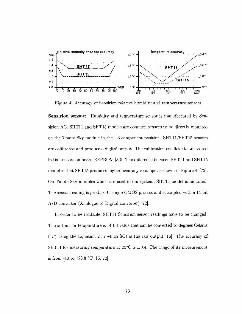
Figure 4: Accuracy of Sensirion relative humidity and temperature sensors
Sensirion sensor: Humidity and temperature sensor is manufactured by Sen-
sirion AG. SHT11 and SHT15 models are common sensors to be directly mounted
on the Tmote Sky module in the U3 component position. SHT11/SHT15 sensors
are calibrated and produce a digital output. The calibration coefficients are stored
in the sensors on board EEPROM [36], The difference between SHT11 and SHT15
model is that SHT15 produces higher accuracy readings as shown in Figure 4 [72].
On Tmote Sky modules which are used in our system, SHT11 model is mounted.
The sensor reading is produced using a CMOS process and is coupled with a 14-bit
A/D converter (Analogue to Digital converter) [72].
In order to be readable, SHT11 Sensirion sensor readings have to be changed.
The output for temperature is 14-bit value that can be converted to degrees Celsius
(°C) using the Equation 2 in which SOt is the raw output [16]. The accuracy of
SHT11 for measuring temperature at 25°C is ±0.4. The range of its measurement
is from -40 to 123.8 °C [16, 72],
73

Temperature = -39.60 + 0.01 * SOt (2)
For relative humidity measurement, the output is a 12-bit value that is not
temperature compensated. The SI unit value for humidity can be calculated from
Equation 3 where SOrh is the raw output of the relative humidity sensor [16, 72].
Humidity = - 4 + 0.0405 * SOrh + ( -2 .8 * 10~6) * (SOrh2) (3)
By using the calculated humidity from Equation 3 and calculated temperature
from Equation 2, the humidity measurement can be corrected with temperature
compensation in Equation 4 [16, 72]. In Equation 4, Tc is the temperature mea-
sured in °C from Equation 2, SOrh is the raw output of the relative humidity
sensor, and Humidity is the uncompensated value calculated in Equation 3.
Humiditytrue = {Tc - 25) * (0.01 + 0.00008 * SOrh) + Humidity (4)
In Table 3, the detailed performance specification of the SHT11 sensor is listed
[72].
Hamamatsu Photo-synthetically Active Radiation (PAR) and Total So-
lar Radiation (TSR) sensors These two sensors are used for measuring the
74

Parameter M I N T Y P M A X Units Humidity Resolution 0.5 0.03 0.03 %RH
8 12 12 Bit Range 0 100 %RH Temperature Resolution 0.04 0.01 0.01 °C
0.07 0.02 0.02 °F 12 14 14 bit
Range -40 123.8 °C -40 254.9 °F
Table 3: Sensirion relative humidity and temperature performance specifications
light. It takes about two minutes for each sensor to be calibrated and sense the
right data. The motes that we have used in our system are equipped with these
light photo-diodes. The diodes are S1087 for sensing Photo-synthetically Active
Radiation (PAR), which is the entire visible spectrum and S1087-01 for sensing
the Total Solar Radiation (TSR), which is the entire visible spectrum expanding
to infrared. Figure 5 shows the photo sensitivity of the light sensors on Tmote
Sky [61].
The TSR and PAR sensor readings are also transfered by using the micro-
controllers 12-bit ADC with voltage of 1.5V. The photo-diodes create a current
through a lOOkOhm resistor. By calculating the raw voltage and converting this
voltage into the current using Equation 5 in which Vsensor is the raw voltage
(1.5V), the current created by photo-diodes is calculated.
Vsensor 100,000
75

200 100 600 800 1000
WAVELENGTH (nm)
Figure 5: Photo sensitivity of the light sensors on Tmote Sky
S1087 light sensors datasheet includes a curve for converting the photo-diode's
current into incident light level (lux or Ix) [61]. The lux is the metric unit of
illuminance [59] for measuring the amount of light that falls on an object. Lux is
the European unit equivalent of the British foot-candle (or lumen). Specifically,
one lux is equal to the amount of light that falls on a one-square-meter surface
which is one meter away from a single candle. Ten lux equals the amount of light
produced by ten candles one meter away [1]. Table 4, shows the equivalence of
real world examples to different lux values [69].
The short circuit current linearity for Si087 and SI087-01 are shown in Figure
6. For calculating the sensed lux by S1087 sensor (sensing Photo-synthetically
Active Radiation (PAR), which is the entire visible spectrum), we use Equation 6.
76

Illuminance Example 0.00001 lux Light from the brightest star(Sirius) 0.0001 lux Total starlight, overcast sky 0.002 lux Moonless clear night sky with airglow 0.01 lux Quarter moon 0.27 lux Full moon on a clear night 1 lux Full moon overhead at tropical latitudes 3.4 lux Dark limit of civil twilight under a clear sky 50 lux Family living room 80 lux Hallway/toilet 100 lux Very dark overcast day 320 lux Recommended office lighting (Australia) 400 lux Sunrise or sunset on a clear day. Well-lit office area 500 lux Recommended office lighting (Europe) 1000 lux Overcast day or typical TV studio lighting 10000 to 25,000 lux Full daylight (not direct sun) 32000 to 130000 lux Direct sunlight
Table 4: Equivalence of real world examples to different lux values
For S1087-01 sensor (sensing the Total Solar Radiation (TSR), which is the entire
visible spectrum expanded to infrared), we use Equation 7 to calculate the sensed
lux. In both equations, I is calculated from Equation 5.
Lux of 51087 = 0.625 * l " 6 * I * 1000 (6)
Lux of S1087 - 01 = 0.769 * 1~5 * / * 1000 (7)
3.3.2 Design
We have used TinyOS 1.2 operating system and NesC programming language in
Cygwin environment for developing the code for the motes of the wireless sensor
77

10°
10-2
10-1
10-6
10-8
10-10
O 10-12
1 0 - H
10*16
(Typ. Ta=25 "C, "A" light source fully illuminated)
Z UJ CE oc D O
Q.
S113 3-01 \
S1133-14
n S1 087-0
N. S1133
/ / / / / / / / /
• \ s 1087
1 0 - 8 1 0 - 6 i O - 4 1 0 - 2 1 00 1 0 2 104 1 06 1 0 8
INCIDENT LIGHT LEVEL (Ix)
Figure 6: Short circuit current linearity
network of our system. The application that we have developed consists of many
components linked together to form an executable. A component provides and
uses interfaces, which are the only point of access to the component. An inter-
face declares two sets of functions called commands and events. Commands are
functions that the component providing the interface should implement. Events
are functions that the component using the interface should implement. Events
are the responses to the commands. For instance, when MultiHop component uses
SendMessages interface to use Send command of LinkLayer component for send-
ing a message, as a result of the completion of the function, event of SendDone
in MultiHop component through SendMessage interface will be called back. This
78
means that the interfaces are bidirectional. However, in graphical view of the com-
ponents relations, the direction of the interfaces usage is shown. For example, if
component A wants to use commands of the component B by interface X, an arrow
from component A to B shows their relation and representing interface X.
In addition, there are two kinds of components: module and configuration.
Modules provide application code, implementing one or more interfaces. Config-
urations are used to assemble other components together, connecting interfaces
used by components to interfaces provided by others. This is called wiring. Every
nesC application is described by a top-level configuration that wires together the
components inside. However, in graphical view of components relations just the
module components would be mentioned.
Figure 7 shows the graphical view of components relations of our motes appli-
cation. In this figure, we have merged all the interfaces between two components to
one interface, omitted the names of the interfaces and just kept the main important
components of the application to be more understandable and clear.
In the motes application, main component is the system component, which
is responsible for starting all other components. The two main components of
our application are BMappl and NetSync. BMappl component is using interfaces
to connect to other components such as sensors, multi-hop communication com-
ponents etc. Main tasks of BMappl component are collecting data from sensors
every 30 seconds, calculating lamp status and generating messages to be sent to
79

Figure 7: Graphical veiw of components relations of the motes application
80

the sink. This component sends the messages to the sink by forwarding them
to the MultiHop component. Another main component is NetSync, which is re-
sponsible for keeping the whole network synchronized for waking up and going to
sleep. NetSync component uses different components such as UartDetect, Timer
and Counter to perform the synchronization. Both MultiHop and NetSync com-
ponents use SensorNetProtocol component. SensorNetProtocol is a unifying link
abstraction for running network protocols over a variety of link layer and physical
layer technologies without changing network protocol implementation [63]. Each
of the components is explained in detail in the rest of this section.
3.3.3 Sensing functions
As we explained in Subsection 3.3.1, there are three sensors mounted on Tmote Sky
modules: SHT11 Sensirion sensor for sensing temperature and humidity, S1087-
01 Hamamatsu sensor for sensing TSR, and S1087 Hamamatsu sensor for sensing
PAR. However, we need to use two components in TinyOS for using these sensors.
HamamatsuC component is used for S1087 and S1087-01 sensors and HumidityC
component is used for SHT11 sensor.
We need to use interfaces wired to the sensors component to get the analogue
readings from the sensors and convert them to digital one. For this purpose, we use
ADC (analogue-to-digital converter) interface to connect to the sensor components.
One ADC interface is defined for each sensor reading as follows:
81

interface ADC as Temperature;
interface ADC as Humidity;
interface ADC as TSR;
interface ADC as PAR;
Temperature interface is used for getting the sensed temperature. Humidity
interface is used for measuring the humidity. TSR and PAR interfaces are used
for measuring the light. TSR and PAR differences are explained in Subsection
3.3.1. For getting data from the sensors, ADC interfaces are wired to appropriate
interfaces of the sensors component. Temperature and Humidity interfaces are
wired to interfaces in HumidityC component and TSR and PAR interfaces are
wired to interfaces in HamamatsuC component. In addition, more interfaces are
used for controlling purposes and error detection of sensors readings. Examples of
wiring between interfaces are as follows:
Impl.Humidity -> HumidityC.Humidity;
Impl.HumidityError -> HumidityC.HumidityError;
Impl.PAR -> HamamatsuC.PAR;
After wiring the ADC and controlling interfaces to the appropriate interfaces of
the sensors component, the timer is defined for determining the intervals in which
sensors have to be sampled. The timer for sensing purpose is set to be fired every
30 seconds. The TimerC component is used in our application for this purpose. In
82

the other words, TimerC component calls Timer.fired command every 30 seconds
to collect the sensor readings. After the timer is fired, each ADC interface is called
to collect the reading. Then, sensor readings will be processed and forwarded to
MultiHop component to be sent to the sink.
In addition, we need to collect the current voltage of the power supply of each
mote. The current voltage of the power supply is used by the end user application
to calculate remaining lifetime of the motes. InternalVolatge interface is used for
connecting to VoltageC component, which returns the current supply voltage. This
value is collected every 30 seconds. For firing the event of reading voltage, we have
used the same timer that is used for the other sensors' reading. The collected
supply voltage is forwarded to MultiHop component with other sensors reading to
be sent to the sink.
As we explained in Subsection 3.3.1, the sensors' reading are not in metric units
and they have to be calculated to be understandable. We do not calculate the
metric units of the sensors reading in the motes for conserving energy. For sending
the raw or calculated sensors reading, the same number of bytes is necessary in
every message to be sent to the sink. Therefore, by calculating the sensors' readings
in the motes, not only we do not lower the routing overhead, but also we use the
motes energy to calculate sensors reading in metric units.
Finally, our application is used for safety as well. All end users are alerted
in case of detection of any light with density or out of visual spectrum such as
83

Min Max Sensors reading Raw data - Metric unit Raw data - Metric unit Temperature 5,460 - 15°C 8,354 - 40°C Humidity 355 - 10%RH 2,703 - 85%RH TSR 0 - 0Ix 88,776 - 25,000/x PAR 0 - Olx 10,923 - 25,000^
Table 5: Predefined thresholds of sensor readings for alerting the end user
infrared, and change in the climate conditions of the building such as temperature
drop or rise. The process of alerting can be performed by checking sensors' reading
to make sure they are not out the predefined threshold before sending to the sink.
The thresholds are defined before programming the motes, then written in the
code of the motes. In case of sensing very high or low temperature, very high or
low humidity, or light with high lux, the motes send the messages every 5 seconds
instead of 30 seconds. The messages are sent more frequently for increasing the
delivery ratio and letting the end user have the up-to-dated status of the event.
The predefined thresholds that we have use in our application are mentioned in
Table 5.
3.3.4 Lamp status (room occupancy)
As we explained in Section 1.2, we are interested in the lamp status (on/off) and
room occupancy of each room. We assumed that the room is occupied when the
lamps of the room are on and the room is empty when the lamps are off. In the
motes application, lamp status is calculated and sent to the sink along with the
sensor readings every 30 seconds. Each time for calculating the lamp status, 100
84

samples of light sensors are collected. Therefore, it is more energy efficient to
calculate the lamp status in the motes than sending all of the 100 samples to the
sink. The 100 samples are collected with 10 milliseconds intervals. The collection
starts one second before sending each message to the sink for having the lamp
status ready with other sensor readings.
For collecting the 100 samples, we defined TimerSenseLight timer, which gets
fired 29 seconds after the timer for the sensors readings is fired. When the
TimerS enseLight is fired, 100 samples of TSR and PAR light sensors are collected
in one second and saved in the mote's memory. Then, calculateLampStat() method
is called and lamp status is calculated. Lamp status is sent to the MultiHop com-
ponent along with other sensor readings for preparing of the message to be sent to
the sink.
Lamp status is calculated based on the fact that power supply of most of
the lamps in offices is Alternating Current (AC). AC flows one way, then the
other way, continually reversing direction. An AC voltage is continually changing
between positive (+) and negative (-). The rate of changing direction is called
the frequency of the AC and it is measured in hertz (Hz) which is the number of
forwards-backwards cycles per second. AC power in Canada has a frequency of
60Hz [9], meaning that electrical signal of AC power take 60 cycles in one second.
The time period for the electrical signal of AC power is the time taken for the
signal to complete one cycle. Figure 8 shows an electrical signal of AC power and
85

Figure 8: Voltage-time graph of an AC power electrical signal
its time period. The time period for AC power in Canada is calculated by Equation
8 to be 16.6 milliseconds.
Time period = — (8) Frequency
Therefore, the lamps which are using AC power in Canada flicker 60 times in
one second. The light generated by lamps are going up and down due to the nature
of AC power. When the electrical signal of AC power reaches its highest peak, the
lamps are acting accordingly and they generate their highest brightness and when
the electrical signal reaches zero, the lamps are generating no light. However, the
persistence of human vision prevents the light to appear flickering as long as the
light flickering rate is fast enough (greater than 20 flickering per second is good if
86

the human vision can tolerate some flickers, but generating flickering with rate of
60 per second avoids any appearance of intensity flicker [78]).
As we explained, the time period of AC power electrical signal is 16.6 millisec-
onds. Thus, the lamps take 16.6 milliseconds to complete one cycle of flickering.
Therefore, we use light sensors to sense light of the lamps every 10 milliseconds
for a period of 1 second to detect the flickering of the light. The lamps are on
when the light is flickering and the lamps are off when the light is steady in a short
period of time. In the other words, we detect the status of the lamps (on/off)
in every room equipped with any kind of lighting system as long as they use AC
power. The system is therefore able to detect the lamp status in the rooms with
windows facing outside (having daylight) as long as light sensors are close enough
to the lamps (less than 2 meters) and they are placed out of direct sunlight.
Moreover, we first tried to detect the lamps status by monitoring the changes
in the level of brightness in the room. This method was working well for the rooms
without the daylight, since the changes in the level of the brightness in such rooms
are very distinguished and limited to two states. The lamps are either switched on
or off. In each state, changes in the level of brightness are very high and unique in
such a way that the level of brightness drops very low sharply when the lamps get
switched off and it rises very sharply when the lamps get switched on. Figure 9
shows examples of changes in the level of brightness in the rooms without daylight.
However, it is a different issue for the rooms with daylight. Figure 10 shows an
87

TS]
439.C
1 & PAR raw rea« ings TS
4391
R & PA R raw ri ladings »*
A t 105.C
Lamps a switched 7 105.1
Lamps a switched * on \
p ' ..... .«..,.„ • * »»»«TOBI«
-229; J TimeO ecood)
-226. ) Time [second]
39! 5.0 40' 1.0 40; 9.0 42C 7.0 4 3 . 7.0 43( 5.0
Figure 9: Changes of TSR and PAR raw readings when lamps are switched on or off in the rooms without daylight
example of changes in the level of brightness in different states in the rooms with
daylight. After several testings and observations, we figured out that there is no
specific pattern applicable to such cases.
During the tests, we found out that when the lamps are on in the room, the
light sensors can sense the light flickers as long as light sensors are close enough
to the lamps (less than 2 meters) and they are out of direct sunlight. However,
the light in the rooms with daylight is steady in very short periods of time when
the lamps are off. Figure 11 shows an example of light sensor readings in the
room with daylight and switched off lamps. From this figure, we can see that even
though the overall light in the room is increasing, but in small periods of time
the differences in sensed light is one or two units. Figure 12 shows an example
of light sensor readings in the room with daylight and switched on lamps. As we
88

oo
Figu
re 1
0: C
hang
es o
f T
SR a
nd P
AR
raw
rea
ding
s w
hen
lam
p is
switc
hed
on o
r of
f du
ring
var
iabl
e cl
oudy
day
in
peri
od
of o
ne h
our
in t
he r
oom
with
day
light

Figure 11: Changes of TSR and PAR raw readings when the light in the room is from Sun only
mentioned before, this figure shows the light from lamps in a short period differs
between 3 to 12 units. Therefore, we calculate the lamp status by collecting 100
samples of light sensors with intervals of 10 milliseconds in 1 second. Then, we
check the differences of each two subsequent sensors readings. If the difference is
from 0 to 3, we add one to the countOFF counter and if the difference is from 4
to 12, we add one to countON counter. Whenever any of the counters reaches 5,
we change the lamp status accordingly and set both counters to 0.
3.3.5 Routing algorithm
The routing algorithm (MultiHop component) of our application is based on the
many-to-one data-collection scenario, since our application is classified under data
gathering and periodic reporting class as we explained in Section 2.1.2. The used
approach is to build one collection tree rooted at the sink. When a node has
data to be collected, it sends the data up the tree. Also, a node forwards the
90

Figure 12: Changes of TSR and PAR raw readings when the light in the room is from both Sun and the lamps
collected data that is sent by other nodes. Messages are inspected as they go
by, to suppress redundant transmissions and to avoid loops. As we mentioned
in Section 2.3, in our system, messages are not inspected for data aggregation,
since the collected data in our system is not redundant. The reason for not having
redundant data in our system is that there is one mote in each room of the building
and it makes all data collected from the motes independent of the others. We
placed one mote in each room due to the small sizes of the rooms. Therefore, by
using data aggregation, not only is the forwarded data not reduced but also, we
have more in mote processing and delay in the network. Moreover, data query is
not applicable in our system because of the class of data gathering and periodic
reporting in which our application is classified. Thus, there is no need to query
any part of the network to get data regarding any specific event.
91

MultiHop routing protocol chooses a parent based on the best link quality to
the root of the collection tree. In this implementation, we have used additive link
qualities, where zero represents a perfect link. A parent's quality is its adver-
tised value, sent periodically via route update messages, plus the quality of the
link between parent and child (lower values are better). The sink in our network
is identified either by its id which is zero or by its connection to the PC. The
sink's quality advertised to the neighbors is set to zero. MultiHop uses Link Qual-
ity Indication (LQI), which is a feature of the CC2420 radio with IEEE802.15.4
standard.
The IEEE802.15.4 standard enables the measurement of link quality between
neighboring nodes in the network. This measurement is in the form of a Link
Quality Indicator (LQI) value reported with each received packet. By averaging
over several LQI values, an estimation of the link quality is obtained and conse-
quently, an estimation of the probability of successful transmission is available to
the MultiHop routing algorithm. The LQI measurement is a characterization of
the strength and/or quality of a received packet, as defined by [27],
Figure 13 shows an example of selecting best route by the motes to the sink
using the MultiHop routing algorithm. In the first step, the sink (mote 0) advertises
link quality with value of zero to its neighbors. In step two, motes 2, 3 and 4 select
the sink as their parent and set the value of their link quality to the sink (e.g.,
link quality of mote 2 to mote 0 is set to value 1). In step three, motes 2,3 and 4
92

advertises to its one-hop neighbors the route update message which has the parent
link quality plus the link quality from themselves to their parent (e.g., mote 2
advertises the value of 1, that is, the sum of its parent link quality, which is 0 and
the link quality from itself to its parent, which is 1). In step four, motes 5,6,7
and 8 select a mote with lowest advertised link quality as their parent (e.g., mote
6 selects mote 3 instead of 2 since the advertised value from mote 3 is less than
the mote 2). Step five shows that whenever there is a tie between the advertised
values, the mote with lower id is selected as parent (e.g., the advertised value from
mote 7 and 8 to mote 9 are the lowest and both are the same, which is 4, therefore
mote 9 selects mote 7 as its parent). In step six, the dashed lines show the two
alternate parents that have been selected by mote 9.
MultiHop uses Sensornet Protocol (SP) as the underlying layer. SP provides
shared neighbor management and a message pool in order to let multiple routing
algorithms run over different link layers together. We explained SP in Subsection
3.3.7. MultiHop sends two kinds of traffic by using the SPC component which
is the implementation of SP: route update beacons it broadcasts, and data mes-
sages it unicasts to the currently selected parent. The broadcast messages are sent
through a unicast round-robin emulation. If the neighbor table in SP has no good
potential parents, MultiHop requests SP to find new neighbors using the SPNeigh-
bor interface. The find command maps to MAC layer 15.4's scan functionality to
repopulate the neighbor table. In our implementation, the neighbor table keeps
93


the information of at most three neighbors.
Given the limited states that motes can store and general need for distributed
tree building algorithms, the MultiHop collection routing protocol encounters sev-
eral challenges. The following are the challenges addressed in MultiHop routing
algorithm:
Loop detection: Routing loops are problems that can happen in the network.
Routing loops generally occur when a node chooses a new route that has a signif-
icantly higher link quality than its old one, perhaps in response to losing connec-
tivity with a candidate parent and also the new route includes a node that was a
descendant. For many-to-one routing over relatively stationary sensor networks,
we believe that it is better to use simple mechanisms to avoid loop formation and to
break cycles when they are detected, rather than to employ heavy weight protocols
with inter-nodal coordination.
MultiHop addresses loops through two mechanisms. First, cycles can be de-
tected quickly when a node in a loop originates a packet and observes it returning.
Once a cycle is detected, it will be broken by discarding the parent by choosing
a new one or becoming disjoint from the tree. The second mechanism is to use
Time-To-Live (TTL) field in the data frame. We defined the TTL to be four times
greater than the parent hop count to the sink. Whenever the message is forwarded
by any mote, the value of TTL is reduced by one unit. The message will be dropped
when the TTL becomes zero. Therefore, the messages cannot be stuck in the loop
95

forever.
Duplicate packet elimination: Duplicate packets can be created upon retrans-
mission when the ACK is lost. Without duplicate packet elimination, the forwarded
duplicates will possibly cause more retransmissions and more contention, beside
wasting energy. This can have disastrous effects over multiple hops, as the dupli-
cation is exponential. For example, if each hop on average produces one duplicate,
then on the first hop there will be two packets, on the second there will be four,
on the third there will be eight and so on.
To avoid duplicate packets, the routing layer at the originating node appends
the sender id and an originating sequence number in the routing header. To sup-
press the forwarding duplicate packets, each parent retains the most recent origi-
nator id and originating sequence number in child entries in the neighbor table.
Implementation
Figure 14 shows the graphical view of components relation of the MultiHop routing
algorithm in our system. The implementation of MultiHop has the following major
parts:
Collection interfaces: The motes can perform three different roles in collection:
producer, snooper and consumer. Depending on their role, the motes use different
interfaces to interact with the MultiHop routing algorithm component.
96

Figu
re 1
4: G
raph
ical
vie
w o
f co
mpo
nent
s re
latio
n of
Mul
tiHop
co
mpo
nent

The nodes that generate data to be sent to the root are producers. The pro-
ducers use the send interface (MultiHop.Send[AM-BMAPPLMSG]) to send data
to the root of the collection tree. The collection identifier is specified as a parame-
ter to send during instantiation. The collection identifier is unique and used in the
mote application and the end user application for identifying the application that
collects the sent data. In the other words, identifier is used to distinguish different
kinds of messages for data transfer or route update. One advantage of using SP
as the under-layer of the routing algorithm is having different applications imple-
mented in the motes for different purposes. As we explained in Subsection 3.3.2,
two components of NetSync and MultiHop are implemented independently over
the SP layer. Figure 7 shows the graphical view of the components relation of the
mote's code and also the independent implementation of NetSync and MultiHop
components. Each of the messages in the motes has its unique identifier. For
instance, the identifier for data collected by BMappl is AM-BMAPPLMSG = 33.
The motes that overhear messages in transit are snoopers. The snoopers use
the receive interface (MultiHop.Snoop[AM-BMAPPLMSG]) to receive a snooped
message. Intercept has a single event which is Intercept.forwardf). A collection
service in other routing algorithms signals this event when it receives a packet
to forward. However, in our routing algorithm because of not having in mote
processing, the routing algorithm calls this event automatically upon receiving a
message to forward. This causes less delay to avoid the message to go to upper
98
level.
Root node (the sink) that receives data from the network is consumer. The
sink uses the receive interface (MultiHop.Intercept[AM-BMAPPLMSG]) to receive
a message delivered by collection and forward it to USB port connected to the PC.
In MultiHop component, the RootControl interface configures whether a node is
a root or not by checking if one of following factors are true, whether the mote
has id number zero or the mote is connected to the PC. The connection and
communication to the PC is handled by UartDetectC component.
Data messages: The data message frame is used by MultiHop component to
send collected data to the sink. The data forwarded from the application layer is
encapsulated in the data field of the data message. The data message has different
fields mentioned in Table 6. In this table, sourceaddr is the id of the last mote
that forwarded the message, originaddr is the id of the mote that collected the
data. For instance, if motel sends its own collected data, both the sourceaddr
and originaddr are 1. However, if motel forwards data message to mote4, the
sourceaddr will be 1 and originaddr will be 4. seqno is the sequence number of
messages sent from the source address, originseqno is the sequence number of
messages forwarded by the mote, ttl is the time duration in which the message
has lived, id is the type of the data message, data field is the collected data by
application layer. The identifier of data messages is AM-MULTIHOPMSG = 8.
99

Field Size(bits) sourceaddr 16 originaddr 16 seqno 16 originseqno 16 ttl 8 id 8 data(BMappl messages) 240 Whole size in bytes 40
Table 6: Data messages structure in MultiHop routing algorithm
BMappl messages: Collected data in BMappl is saved in the BMapplMsg data
structure. Then, BMapplMsg will be forwarded to the MultiHop component to
be encapsulated in a data message frame. BMapplMsg structure is mentioned in
Table 7. Most of the fields are self explanatory except the neighbor related fields.
neighborsize field is the number of neighbors of the mote that their information is
sent in this message. Each mote saves information of up to maximum eight neigh-
bors since its radio neighborhood size is 8. However, neighborsize can be from one
to maximum three in order to avoid very big messages. Having information about
maximum three of the neighbors is enough to draw and analyze the connectivity
status of the whole network and each mote. The two arrays of neighbors[3] and
quality[3] have the id of the neighbors and quality of the links to those neighbors.
The identifier for collected data in BMapplMsg is A M.BMA PPL MSG = 33.
Route update beacons: Route update beacons are used by MultiHop com-
ponent for updating its neighbor table. Beacons are sent every 30 seconds to
single-hop neighbors. Table 8 shows the fields of the beacons, parent is the id of
100

Field Size(bits) seqno 32 dataOTemp 16 datalHum 16 data2TSR 16 data3PAR 16 data4LampStat 8 data5IVolt 16 parent 16 neighborsize 8 neighbors[3] 3*16 quality[3] 3*16 Whole size in bytes 30
Table 7: BMappl message structure in MultiHop routing algorithm
Field Size(bits) parent 16 cost 16 hopcount 16 Whole size in bytes 6
Table 8: Route update beacons structure in MultiHop routing algorithm
the mote itself, cost is the link quality of the route from the mote itself to the
sink, hopcount is the hop count from the mote to the sink. The identifier of route
update beacons is A M.BEA CON MS G = 7.
MultiHopDataM and MultiHopLQIM components: MultiHopDataM mod-
ule manages the data flow of messages, and uses SP to queue outgoing messages
for transmission. This module uses link quality provided from MultiHopLQIM
as well as network-level information to decide which neighbor is the next routing
hop. MultiHopLQIM module is link estimator for MultiHop router. It assists Mul-
tiHopDataM in assigning routes and forwarding messages by using Link Quality
101

Indications (LQI).
Route Statistics and RouteControls components: Both components are
used to keep track of routing information and make route selection decisions. When
a Send component wants to send a packet from the application layer, it passes it
to either RouteStatistics or RouteControls components for its routing information
to be filled in. This way, the Send component is entirely unaware of the routing
header structure.
3.3.6 Synchronization
The power consumption of the motes is in its maximum value when the radio
transceiver is on. The power consumption of the Tmote Sky in different operating
conditions is shown in Table 2. For energy conservation, we minimize the amount
of time that the radio has to be on. The motes in our network transmit and
receive for 100 milliseconds every two seconds. The ratio of the time in which the
mote's radio transceiver is on to sum of the time in which the radio module is on
or off is called the duty cycle. Therefore, the duty cycle of the radio module of
the motes is 5%. In order to have an appropriate functionality in the network,
all motes are synchronized together in such a way that they turn on and off their
radio transceiver for transmitting and receiving at the same time.
In the rest of this section, we explain the calculation of the required duty
cycle and the estimated lifetime of the motes. Then, we describe the NetSync
102
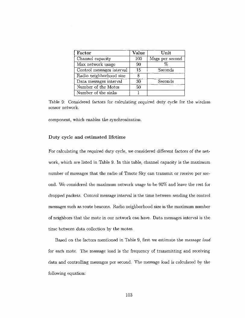
Factor Value Unit Channel capacity 100 Msgs per second Max network usage 90 % Control messages interval 15 Seconds Radio neighborhood size 8 Data messages interval 30 Seconds Number of the Motes 50 Number of the sinks 1
Table 9: Considered factors for calculating required duty cycle for the wireless sensor network.
component, which enables the synchronization.
Duty cycle and estimated lifetime
For calculating the required duty cycle, we considered different factors of the net-
work, which are listed in Table 9. In this table, channel capacity is the maximum
number of messages that the radio of Tmote Sky can transmit or receive per sec-
ond. We considered the maximum network usage to be 90% and leave the rest for
dropped packets. Control message interval is the time between sending the control
messages such as route beacons. Radio neighborhood size is the maximum number
of neighbors that the mote in our network can have. Data messages interval is the
time between data collection by the motes.
Based on the factors mentioned in Table 9, first we estimate the message load
for each mote. The message load is the frequency of transmitting and receiving
data and controlling messages per second. The message load is calculated by the
following equation:
103

Message load = f\ + f2
where f\ is the frequency of control messages and /2 is the frequency of data
messages. f\ is calculated as follows:
Number of control messages Control messages interval
The number of control messages, which includes synchronization and routing
messages, is independent of the size of the network. / 2 is calculated as follows:
Number of data messages Data messages interval
The number of data messages is dependent on the size of the network. In the
worst case scenario — the messages of all motes should be forwarded by one mote
to the sink — if the number of the motes is N, the number of data messages to
send and receive by one mote is 2N-1.
Then, we calculate the duty cycle as follows:
Message load Duty cycle =
('Channel capacity) (Maximum network usage)
104

where channel capacity is 100 messages per second and maximum network
usage is considered 90 %.
Moreover, for calculating the lifetime of each mote, we use the power consump-
tion information of Tmote Sky in Table 2. Even though the required duty cycle for
our application is 5%, we calculate the lifetime of the motes in the network with
three different duty cycles: 100%, 5% and the lowest 1%. Our network can run
with 1% duty cycle if the data messages interval is changed to 360 seconds (6 min-
utes). In the network with 100% duty cycle, the motes are running in full power
(100% duty cycle), meaning that their radio transceiver is always on and ready to
transmit and receive. In the networks with 5% and 1% duty cycle, the motes are
running in low power, meaning that their radio transceiver is on only in the 5% or
1% of the time. For this calculation, we consider 20mA for the active current of the
motes in which its radio module is on and 10//A for the sleep current of the motes
in which its radio module is off. In addition, we count the energy source as two
Eveready A A Alkaline batteries with 2600 mAH (2600 milli-Ampere-Hour) [20],
The results of the calculation are shown in Table 10. The calculation of the mote's
lifetime is done as follows:
Average current = (Active current)(Duty cycle)-\-(Sleep current)(1—Duty cycle)
Batteries energy Life time of the motes = — — Average current usage
105
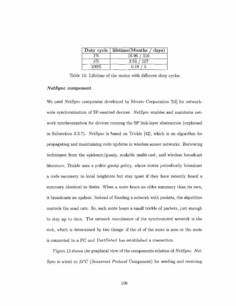
Duty cycle lifetime(Months / days) 1% 16.96 / 516 5% 3.53 / 107
100% 0.18 / 5
Table 10: Lifetime of the motes with different duty cycles
NetSync component
We used NetSync component developed by Moteiv Corporation [53] for network-
wide synchronization of SP-enabled devices. NetSync enables and maintains net-
work synchronization for devices running the SP link-layer abstraction (explained
in Subsection 3.3.7). NetSync is based on Trickle [42], which is an algorithm for
propagating and maintaining code updates in wireless sensor networks. Borrowing
techniques from the epidemic/gossip, scalable multi-cast, and wireless broadcast
literature, Trickle uses a polite gossip policy, where motes periodically broadcast
a code summary to local neighbors but stay quiet if they have recently heard a
summary identical to theirs. When a mote hears an older summary than its own,
it broadcasts an update. Instead of flooding a network with packets, the algorithm
controls the send rate. So, each mote hears a small trickle of packets, just enough
to stay up to date. The network coordinator of the synchronized network is the
sink, which is determined by two things: if the id of the mote is zero or the mote
is connected to a PC and UartDetect has established a connection.
Figure 15 shows the graphical view of the components relation of NetSync. Net-
Sync is wired to SPC (Sensornet Protocol Component) for sending and receiving
106

messages through this component. Usage of SPC makes it easy to implement and
avoid any interference with the MultiHop component, while both messages can be
transfered to lower layers with no more code development. Whenever NetSync
has a message to send, it pushes the message to SPC by using SPSend interface.
Also, whenever a message for NetSync is received at the mote, SPC delivers it
to NetSync through RecieveMsg interface. NetSync uses other components for en-
abling timers, counters and connection recognition to the USB port. In order to be
adapted to our application we have made some minor changes such as decreasing
the interval between synchronization beacons. The reason for this change is that
the clock drift makes the motes go out of sync. The main clock on the Tmote Sky
runs on an internal DCO, which has a lot of frequency error (could be about 10%),
unless the error is corrected through periodic recalibration with the crystal. We
believe that the timers use the 32KHz crystal in TinyOS, which leads to a huge
frequency error. This means that if we do not resynchronize the timer periodically,
the clock drift could be unbounded.
3.3.7 Sensornet protocol
We used Sensornet Protocol (SP), which is a unifying link abstraction for run-
ning network protocols over a variety of link layer and physical layer technologies
without changing network protocol implementation [63].
107

Figu
re 1
5: G
raph
ical
vie
w o
f co
mpo
nent
s re
latio
n of
Net
Sync
co
mpo
nent

Figure 16 shows the graphical view of the components relation of SPC (Sen-
sornet Protocol Component). In SPC, messages are transmitted using the SPSend
interface and next messages are handled through the SPSendNext interface. In
order to send a message on a particular message identifier type (such as type 5),
we wire our network protocol to SPSend[5j. The SP message pool holds on to
a message and its corresponding packets until it may be sent over the channel.
Fields of each SP message (sp-messageJ,) can not be directly accessed. Instead,
they can be set using the parameters of the SPSend interface.
Reception is on a per-packet-basis (not per-message-basis like SPSend). Pack-
ets are immediately dispatched to higher layer services based on message identifier
type. It means if there is a message bigger than 125 Bytes (the maximum size
of message that can be transmitted by the radio transceiver of Tmote Sky), the
network protocol (higher level) is responsible to break it down and put it together
in the other end. SP Neighbor Table is accessed through SPNeighbor interface.
We wired the MultiHop component with the parameter unique (SPNeighbor) to
SP Neighbor Table. Each service then has its own identity for controlling the
insertions, removals, and changes to entries in the SP Neighbor Table.
The other main components of SP are as follows: SPM is the implementation
of the primary state machine of SP for handling messages, both transmitted and
received. SPM works with other components to send messages from the pool when
appropriately notified by the SP Neighbor Table or the link protocol. SPDataM
109
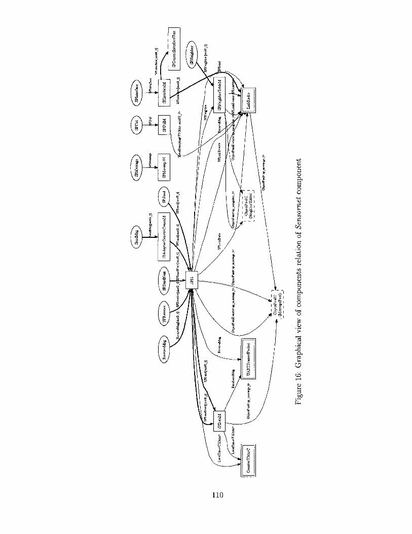

sets the data fields of SP messages and TinyOS packets. It also maintains the
SP Message Pool. SPUtilM is the implementation of the utility functions (link
estimation and time stamping) for SP. SPNeighborTableM is the implementation
of SP's Neighbor Table and associated management functions. SPInterfaceM is
the SP Interface/Device query interface from Radio and USB port connection
when the mote is working as the sink. SPAdaptorGenericCommM is an adapter
that converts standard packets into SP messages, dispatches them to SP, and then
decomposes the messages back into packets after transmission.
3.4 Gateway/server
As we explained in Section 3.2, our system has a gateway/server, which enables
data messages from the sink to be forwarded to end user applications and archived
in the database. The gateway/server is connected to the sink through a USB port
and acts as a server for the end user applications. It should be connected to the
end user and database through the Internet.
In this section, first we explain the design of the gateway/server. Then, we
break down the main components and functionalities of it.
3.4.1 Design and features
Figure 17 shows the package diagram of the gateway/server. The three main
packages of the gateway are com.concordia.bm.motes, com.concordia.motesbridge,
111

rtet.tiriyos.utiJ
Messenger PrintStreamMessenger
coRMoncw&MnoteiiHidge
CterttsHandler
frfoteslnterface •UartDetect
I V i i
nettinyos.message i i M'
.GiqtttoMF Dispatcher Message
com.concordia.bm,motes .GiqtttoMF Dispatcher Message BMapplMsg
MultiHopMsg UartDetectConsts UartDetectMsq
MessageListener MotelF LlnkedMessaoe
BMapplMsg MultiHopMsg UartDetectConsts UartDetectMsq
i i i i i i com.concordia.bm.db
DBConnection DBLinkTable DBReadingTable DBUodateQuery
Figure 17: Package diagram of the gateway/server
and com.concordia.bm.db.
The com.concordia.bm.motes package includes classes for creating and access-
ing messages of motes. There are two kinds of messages: USB connection messages
and data messages. USB connection messages are used to establish synchronized
connection between the gateway/server and the sink. UartDetectMsg and UartDe-
tectConsts are the classes for accessing and generating USB connection messages.
Data messages are the collection of data from each mote in the network. They
112

consist of the header and data field. The header of data message is accessed by
MultiHopMsg class. Data field of data message is accessible by BMapplMsg class.
The com. concordia. motesbridge package is responsible for connections to the
sink and to the end user applications. In this package, MotesBridge is the main
class, which initiates the gateway/server application. The initiation is done by
using UartDetect class to find the connected mote to the PC and then establishing
the connection. Then, the Moteslnterface class makes a thread for listening to the
sink and extracting data messages from UartDetectMsg. This class interprets the
correctness of data messages. Concurrently, Moteslnterface establishes a server for
listening to the clients, which are the end user applications. Whenever a client (the
end user application) connects to the server successfully, one thread will be created
for the client and handed over to Clients Handler class. This class is responsible
for transmitting and receiving messages to and from each client.
The com.concordia.bm.db package is implemented to handle the database con-
nection and includes all queries, which are used in the end user application for
data archiving.
The gateway/server uses six auxiliary packages from TinyOS operating system
for utility functions and one external library file, which is comm.jar for communi-
cating through USB port. Complete class diagrams and package diagrams of the
gateway/server are shown in Appendix B.
113

3.4.2 Sink connection
The gateway/server communicates with the sink through the USB connection syn-
chronously First, the gateway/server figures out which USB port is connected to
the sink by scanning the ports. After finding the port, the gateway/server con-
nects to the Tmote Sky with the baud rate of 57600. After the establishment
of the connection, one thread gets set to receive the messages from the sink and
another thread gets set to send messages to the sink. Then, received messages will
be forwarded to all connected clients.
3.4.3 Internet connection
The gateway/server is running as a server and can accept connections from many
clients. The connection is implemented based on reliable and connection-based
TCP/ IP protocol. Since TCP/IP is streaming the data, we cannot send messages
in packets. Therefore, we used in-order-delivery feature of this protocol and extra
header sent with each message to let the client distinguish separate messages. In
the other words, we extract four pieces of information from each message and
send them as the header of each message in the stream pipe. At the other end,
client uses this information to distinguish separate messages. The four pieces of
information are the message identifier, the message length, length of data field in
the message and base offset of data field in the message. One thread is responsible
for each client for sending and receiving the data.
114

:":•.' ' motes: PK id
.11 .iikS'V
1 2 *
room PK datetime
1 2 *
isbase PK, FK1 childid
1 2 * dateti m estarting
PK, FK2 parentid 1 2 * start in gpo wer lq currentpower isparent timetofailure
dateti meseen by appl datetimelastmsgrec temp hum lightlTSR
PK datetime light2PAR PK, FK1 PK
id seqno l 1 islampon
power parent parentlq
temp altparentl hum altparentllq lightlTSR altparent2 light2PAR altparent2lq islampon seqno
locx locy
Figure 18: The database schema for bm database
3.4.4 Database
In the gateway/server, whenever a new message from a mote in the network is
received and interpreted, the interpreted data has to be archived in the database
for later retrieval and analysis. Therefore, we have defined a database in MySQL
server 5.2. Figure 18 shows the schema of the designed database. As shown in the
database schema, we defined three tables in this database. The fields and features
of three tables are explained below:
115

Motes table: This table has one row for each mote in the wireless sensor net-
work. Therefore, the primary key of this table is id of the motes. This table keeps
the information for the last status of each mote. The information archived in this
table for each mote is explained in detail in Subsection 3.5.3. In this table, there
are fields that are updated upon receipt of each message from the mote such as
received messages, temperature, humidity, etc. However, there are other fields that
are updated more rarely such as Starting date and time. The data in this table is
retrieved by the end user application for different purposes in the application such
as initiating the object for newly seen motes in the visualization process, filling
the drop down list with list of motes in database in query and analysis tabs, and
updating the last status of each mote in database based on newly received data
message.
Readings table: This table is used for archiving specific interpreted data from
every messages received from the motes. The interpreted data archived in this
table includes temperature, humidity, brightness by TSR sensor, brightness by
PAR sensor, lamp status (room occupancy), and sequence number. The message
interpretation is explained in Subsection 3.5.3. For each row in this table, besides
the interpreted data from the message, the date and time of the message reception,
and the id of the sender mote is archived in this table. For avoiding any redundant
data, we defined combined primary key, which includes date and time, id and
sequence number for this table. The foreign key of readings table is its id column,
116
which is pointing to the id column of the motes table.
In this table, one row is inserted whenever the new message is received from
any mote in our wireless sensor network. The data in this table is retrieved by the
end user application for analysis by the users, which are responsible for building
management through Building Managing Query & Analysis tab, which is explained
in subsection 3.5.7.
Links table: All reported link information from the network gets archived in
this table. Each link has the following information: id of child mote, id of parent
mote, quality of the link, and whether the link is pointing to the current parent
or alternative parent. Link information is reported by the messages received from
the motes. Every message includes the link information to its current parent and
at most two of its alternative parents. The interpretation of link information is
explained in detail in Subsection 3.5.3. Therefore, the date and time of the message
reception is archived in the table. The primary key of this table is the composition
of date and time of message reception, id of parent mote and id of child mote. The
foreign key is the id column of motes table.
In the Links table, at least one and at most three rows are inserted whenever
a new message is received from any mote in our wireless sensor network. Data in
this table is retrieved by end user application for analysis by the users, which are
responsible for network administrating through Network Administrating Query &
Analysis tab, which is explained in Subsection 3.5.8.
117

C: \cygwin\opt\t lie s is_app\MotesBridge--uer002 >C: \cygwin\bin\bash.exe — tliesis_app/MotesBridge-uer002/bin/bin Gateway Application Detected note on C0M24 Running Gateway Applicaiton serialPC0M24:57600: resynchronising Listening for client connections on port 9001 new client at localhost <127.0.0.1> connected! Clients = 1 RFromMotes= 26 UToMotes= 0 RFromClients= 0 SToClients= 13.
-login /opt/
I d
Figure 19: Gateway/server user interface
Finally, we have to mention that depending on the combination of the criteria
and the category of analysis for archived data selected by the user, the end user
application generates the required query and retrieves the requested data.
3.4.5 User interface
The gateway/server provides different information regarding the number of mes-
sages sent or received and connectivity status of the gateway/server to the clients
and the sink. It also provides information about any malfunction in the applica-
tion such as the receipt of corrupted messages from the sink or any inserting and
updating problem with the database. Figure 19 shows the user interface for the
gateway/server application.
118

3.5 End user application
The end user application is implemented in order to satisfy the user requirements
mentioned in Subsection 1.2.1. The end user application is connected to the gate-
way to receive data messages and queue them for processing. Queued data mes-
sages are interpreted for wireless sensor network visualization and analysis. In
the rest of this section, we explain the design and functionalities of the end user
application.
3.5.1 Design
The end user application consists of eight main packages, six auxiliary packages and
ten auxiliary external libraries. A partial package diagram of the main packages is
shown in Figure 20. The auxiliary packages are from TinyOS operating system for
utility functions to interpret data messages. The auxiliary external libraries can
be categorized by their usage into database connection, topology visualization and
data scaling. Appendix B includes complete class diagrams and package diagrams
of the end user application. The packages that we implemented for our application
are summarized below:
com.concordia.bm: This package is the main package of the end user applica-
tion. It initializes the end user application and connects all packages together. In
addition, auxiliary classes for file handling, date and time calculation, mote data
119

Figure 20: Package diagram of the end user application
120

calculation, and messages and alert rendering are implemented in this package.
com.concordia.bm.client: This package is responsible for connection to the
server. It also distinguishes separate messages from the stream connected to the
TCP/IP layer and then queues them for processing.
com.concordia.bm.topology: This package includes the classes responsible for
data messages interpretation to enable the following tasks: visualizing real time
network connectivity graph (topology), checking individual mote's information
for correctness, updating tables and inserting new data in database by using
com.concordia.bm.db package.
com.concordia.bm.chart-. This package contains the implementation of the
scaling of real time data from the motes and retrieved data from database. More-
over, the panel including the charted data is generated in this package and handed
over to the com. concordia. bm.gui package to be placed in main frames of the scaling
tab.
com.concordia.bm.gui: This package is used for forming the GUI for the end
user application including main frames and tabs. This package is used for all
of the user interfaces except the one for server connection, which is enabled by
com.concordia.bm.client package and the one for topology visualization, which is
implemented in com.concordia.bm.topology.
121

com. concordia. bm. motes: This package includes classes for accessing and gen-
erating data messages structure to enable com.concordia.bm.topology to interpret
the messages.
com.concordia.bm.db: This package is implemented to handle the database
connection and includes all queries, which are used in the end user application for
data retrieval.
3.5.2 Server connection
Figure 21 shows the frame for server connection. In this frame, users enter the IP
address of the server (the gateway) and appropriate port number for the gateway
application to connect to the gateway. Users can connect to and disconnect from
the gateway from this frame without any interruption in the application since
the server connection is handled by one separate thread. All messages regarding
connection confirmation, disconnection and any changes in the connection such as
full buffer and server interruption is shown in the messages panel. The messages
panel is described in Subsection 3.5.5.
After connection establishment with server, the data stream is received from the
stream attached to the TCP/IP layer. Messages are recognized individually based
on the header that we defined for each data message in Subsection 3.4.3. Then, data
messages are reconstructed with classes in com. concordia. bm.motes and queued in
BM.newMessages data structure, which is defined as a static vector. Therefore, for
122

J J J oar. Server IP:
Server Port:
1 2 7 . 0 , 0 , 1
9 0 0 1
Connect Disconnect
Figure 21: Server connection frame
different threads to have shared access to its contents and avoid thread interference
and memory consistency errors, we have used the synchronization tool in Java.
3.5.3 Message interpretation
After the messages are queued in BM.newMessage vector, the Update class in
com.concordia.bm reads the messages and forwards them to three different meth-
ods. Messages are forwarded to readingsDriver.update(msg) and linkqualityDriver.
update(msg) for charting and topologyDriver.update(msg) for visualization. The
message interpretation is done in com.concordia.bm.topology package and then,
the data is available to other packages.
For each mote in the wireless sensor network, one thread is created in the end
user application. Each thread is responsible for the visualization, charting, new
message interpretation, and database update of the mote. For message interpreta-
tion, the classes in com.concordia.bm.motes are used to extract the raw data from
different fields of the message. For each mote in the end user application, there is
123

different information, which is archived in the database, extracted from the mes-
sages or generated by the end user application. This information is provided for
the users and the application for different purposes such as visualization, network
analysis, etc. The provided information includes the following fields:
Mote ID: It is the id of the mote which has sent the message. This value is
extracted from the message to determine the source of the message. Then, the
information of the determined source is updated.
Room number: It is the description of the room or location in which the mote is
placed. This field can be changed by the user in the application. Room information
is saved in the database for letting the user have the information for later usages.
This field is used for making the application more readable in the way that, the id
of the mote will be accompanied by its corresponding room information.
Is Base: This field is used for recognizing the sink from other mote. We have to
have a way to distinguish the sink from the other motes in the end user application,
since the sink in our wireless sensor network can have any id due to the fact that
any mote can be sink if it satisfy one or both of the following conditions: id number
equal to zero or established connection to the sink.
Starting date and time: It is the date and time of the first deployment of this
mote in the building. This field is set once in the application when the first message
124

of the mote is received by the application and it will never change until the power
source of the mote is changed to the higher one. Every time the application is
restarting, the value for this field is retrieved from the database. This information
is used with three other pieces of information to calculate the linear estimation of
Time to failure of the mote. Three other pieces of information are Starting power,
Current power and date and time of the last received message.
Starting power (V): This field is set at the same time with Starting date and
time information. Its value is the voltage of the mote's power source when it has
been placed in the building for the first time. This information is used with other
information for calculating the linear estimation of Time to failure of the mote.
The Starting power is retrieved from database whenever the end user application
is started. If the mote's power increases at least 0.2 voltage due to renewing the
batteries of the mote, the Starting power value will be changed to the current
voltage. At the same time, Starting date and time of the mote is updated to
current date and time.
Current power (V): This field is the current power of the mote in voltage.
Based on Subsection 3.3.1, Starting power and Current power are calculated in
the application.
Time to failure (days): In our application, the Time to failure for each mote
is the estimated number of days for which the mote is operational. Tmote Sky

motes are operational with a supply voltage of at least 2.0V [36]. In the end user
application, the current supply voltage of each mote is received by its message.
Therefore, we can calculate the estimated Time to failure of the motes based
on their current power and the voltage performance of the motes' power supply,
which is two AA Alkaline batteries [20]. The Time to failure of the motes can
not be calculated without considering the batteries brand since the chemistry and
internal resistance of individual batteries from different brands are not the same.
In addition, we can not calculate the exact Time to failure of each mote due to
the dependency of the voltage performance of the supply batteries to the voltage
and current drainage, and temperature [20].
Each mote's power consumption with radio on is 20mA and with radio off is
10//A. Therefore, the mote with 5% duty cycle consumes about 1009.5//A (almost
equal to 1mA). Based on the data sheet of Eveready AA Alkaline battery, with
continuous current drainage of 1mA at temperature of 21°C, the battery voltage
reaches IV in 2600 hours [20]. Thus, the supply power of the motes, which is 2
such batteries is reaching its minimum useful voltage level, which is 2V in 2600
hours. We can define the equation for calculating the remaining lifetime of the
mote based on its current batteries' voltage by using the following equation:
v „ (V2 ~ Vi) , v x Y - y i = t r(A - xi) (.X2 - Xi)
In above equation the Y is the cut off voltage of two batteries and X is time passed
126

in hours to reach this voltage. We have two data points of the equation, which are
,2/1)—(0,3) and (x2,y2)=(2600,2). Therefore, by using the two data points, the
equation will become as follows:
X = {3- y)2600
Then, we can calculate the remaining lifetime by subtracting the result of above
equation from the calculated lifetime of the motes from Subsection 3.3.6. In Sub-
section 3.3.6, we calculated the lifetime of each mote for three different duty cycles
(100%, 5% and 1%) based on the current consumption by the motes and the sup-
plied current per hour by the batteries. The required duty cycle for our network
is 5% by which the calculated lifetime of each mote is 107 days (2568 hours).
Therefore, the Time to failure of the motes in hours is calculated as follows:
TimetoFailure(hrs) = 2568 - (3 - y)2600
= 2600F - 5232
2600^ - 5232 TimetoFailure(days) =
24
Seen by appl on (Date and time at which the message is seen by the
application): The value of this field shows the time and date in which the end
127

user application has been (re)started and received the mote's message. This field
is set at each starting time of the end user application and will never change until
next restart. This piece of information is used to determine how long the real time
number of received messages and lost messages is calculated for.
Last msg received on (Date and time of last received message): This
field is updated whenever a message is received from the mote (every 30 seconds).
This field is used for calculating Time to failure of the mote and checking the date
and time of last status of the mote.
Temperature (°C): This information is extracted from the mote's message ev-
ery time a new message is arrived. The unit for this field is °C. Based on Equation
2 in Subsection 3.3.1, we implemented the real time calculation of Temperature
field.
Humidity (%): This field is the last reported true humidity of the room in which
the mote is placed. The unit of this field is percentage. Based on Equations 3 and
4 in Subsection 3.3.1, the real time calculation of true humidity is implemented in
our application.
Brighness (Lux): In each message from the mote, there are two fields contain-
ing data for brightness calculation. These two fields are lightlTSR and light2PAR.
These fields have the value of the room brightness in which the mote is placed.
128

Although we archive the calculated brightness from the value of both fields in
the database, the value from TSR sensor is just used to show the measurement
of brightness in the graphical user interface due to its higher accuracy and range
of light spectrum coverage than PAR sensor. Based on Equations 5, 6 and 7 in
Subsection 3.3.1, we implemented the real time calculation of brightness from TSR
and PAR sensors readings.
Lamp status (room occupancy): This field determines the status of the lamps
(on/off) in the room. The status of the lamp is used for two purposes, energy usage
and room occupancy monitoring. For determining room occupancy, we used the
status of the lamp in such a way that when the lamps are on the room is full and
when the lamps are off the room is empty. The calculation of the lamp status is
done by the mote itself and just the result is sent to the end user application. The
calculation of lamp status is explained in Subsection 3.3.4.
Parent id and link quality: Parent information of the mote is provided by
the message. It determines which mote in the network is considered by the mote
as its next one-hop forwarding neighbor. Parent link quality is the quality of the
link from the mote to its parent. These information is also used for visualization
purposes.
Alternative parents ids and link qualities: In each message, in addition
to the parent id and link quality, information about maximum two of the mote's
129

other neighbors is also sent to the end user application. The information about
each neighbor includes their ids and link quality. The values of these fields in the
end user application are updated with reception of every message. They are used
to draw the connectivity graph of the network and analyze the connectivity of each
mote in the network.
Sequence number: The sequence number and id of the mote together are used
to calculate the received and lost messages, and drop redundant data messages
delivered to the end user application. Sequence number is extracted from the
BMappl message encapsulated in data message.
Number of received and lost messages: These fields are calculated for every
mote in real time in the event of new message reception. Based on every message's
sequence number, the end user application can calculate the number of received
and lost messages since the start time of the end user application.
X and Y coordinations: These two fields are the coordinates of the mote lo-
cation in the visualization panel. These fields are used for making the visualization
panel more user friendly, in such a way that if the user drags and drops the motes
in this panel, rotate the whole network or change the angels of it, the values of
X and Y coordinations of each mote is updated accordingly and archived in the
database. Then, in case of restarting the program, the motes will be shown on the
panel in the last place they have been left before the application was closed.
130

All above mentioned information for each mote is provided for the end user.
Figure 22 shows the graphical user interface for showing the information of the
selected mote. The user can see the information of any mote by selecting the
mote from the drop down menu or by clicking on it on the visualization panel. In
addition, the end user can modify the room information of each mote by entering
the new information in the text box in the panel and then, clicking on Update
Selected Mote button. The new Room number will be updated for the mote in the
database and visualization panel.
The user not only can see the information of an individual mote (room), he/she
can also see the information of all motes (rooms) together by clicking on the button
named All Motes Overview, which causes a frame titled All Motes Overview to be
opened as shown in Figure 23. This frame shows the information of all active motes
(rooms) in a table format based on real time data provided by last received message
from each mote in the wireless sensor network. The motes can be sorted by their id
or each individual field by clicking on the header of each column. In addition, the
user can replace the columns position in the table for better readability. Moreover,
the columns width can also be widened or shortened. Furthermore, this frame
provides the following functionalities over the table:
• Print: The table can be printed directly from the application.
• Save: The user can save the table in a format readable by Microsoft Excel
application for further analysis, adjustment or later access.
131

Selected Mote Details
Mote ID
Room #
Is Base
Starting on
Starting Power(V)
Current Power(V)
Time To Failure(Days)
Seen by Appl on
Last Msg Recieved on
Temprature(C)
Humidity(%)
Brightness(Lx)
Lamp Status
Parent
Parent LQ
Alternative Parent 1
Alternative Parent 1 LQ
Alternative Parent 2
Alternative Parent 2 LQ
Last Seq No
X Axis in Panel
Y Axis in Panel
Msgs Received
Msgs Lost
8165 . v .
EV8165
No
08/09/30,15:50:57:234
3.24
2,989
249
08/12/02,19:28:40:187
08/12/02,19:33:53:421
20.640001
29.720776
34.332275
OFF
8161
90
8143
64
8173
380
136
650.0
100.0
11
0
Figure 22: The graphical user interface for showing the information of selected mote
132
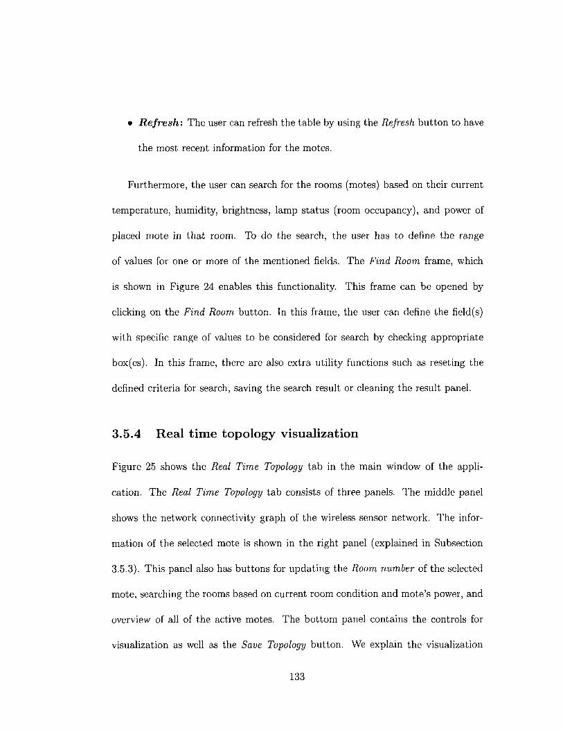
• Refresh: The user can refresh the table by using the Refresh button to have
the most recent information for the motes.
Furthermore, the user can search for the rooms (motes) based on their current
temperature, humidity, brightness, lamp status (room occupancy), and power of
placed mote in that room. To do the search, the user has to define the range
of values for one or more of the mentioned fields. The Find Room frame, which
is shown in Figure 24 enables this functionality. This frame can be opened by
clicking on the Find Room button. In this frame, the user can define the field(s)
with specific range of values to be considered for search by checking appropriate
box(es). In this frame, there are also extra utility functions such as reseting the
defined criteria for search, saving the search result or cleaning the result panel.
3.5.4 Real time topology visualization
Figure 25 shows the Real Time Topology tab in the main window of the appli-
cation. The Real Time Topology tab consists of three panels. The middle panel
shows the network connectivity graph of the wireless sensor network. The infor-
mation of the selected mote is shown in the right panel (explained in Subsection
3.5.3). This panel also has buttons for updating the Room number of the selected
mote, searching the rooms based on current room condition and mote's power, and
overview of all of the active motes. The bottom panel contains the controls for
visualization as well as the Save Topology button. We explain the visualization
133

Figu
re 2
3: T
he g
raph
ical
use
r in
terf
ace
for
show
ing
the
info
rmat
ion
of a
ll m
otes

Fljj'
f fH
O/jl
Q
uer
y
0 Te
mpe
ratu
re(C
):
• B
right
ness
(Lx)
:
Q
Lam
p St
atus
:
• M
ote
Pow
er(V
):
Find
Roo
m
20
0 H
umid
ity(%
): 25
From
: To
:
21
V 30
Res
et
v
Clos
e
Res
ults
4 M
otes
fou
nd:
Mot
e: 8
173
,ln R
oom
: E
V81
73
me
: 81
65 ,
ln R
oom
: E
V81
65
Mot
e: 8
169
,ln R
oom
: E
V81
69
Mot
e: 8
187
,ln R
oom
: E
V81
87
Save
Res
ults
a,
Cle
ar R
esul
ts
Figu
re 2
4: T
he g
raph
ical
use
r in
terf
ace
for
find
ing
the
room
s w
ith d
efin
ed c
rite
ria

and controlling panel in this subsection.
In the connectivity graph of the network, each vertex represents one mote in
the wireless sensor network. All motes in the visualization panel are shown in
red, except the sink, which is shown in blue. Each directed edge represents the
link from the mote to its one-hop neighbor motes (parent and alternative parents).
The link from the mote to its parent is shown in black and the links from the
mote to its alternate parents are shown in gray. Each mote has exactly one parent
except the sink which does not have any parent. In addition, each mote has at
most two alternative parents. All black links together show the collection tree.
The collection tree is rooted in the sink. Moreover, all links together show the
connectivity graph of the network. The weight of each directed edge shows the
link quality from the child to the child's parent. The lower this value is, the better
the link quality would be.
In the visualization panel, the background picture is the map of a specific floor
of the building. Over the floor map, the vertices are placed over the rooms in which
the motes are placed. The end user has many functionalities in the visualization
panel by interacting directly with the panel and by using the control panel, which
is shown in Figure 26. These functionalities are as follows:
• Changing the update frequency for topology: The user can change the
frequency for updating the network topology visualization by using GUI Up-
date Frequency sliding bar. The network topology visualization is updated
136

File
O
ptio
ns
Rea
l tim
e To
polo
gy !
Rea
l tim
e D
ata
Cha
rtpi
g •'.'
Rea
l tsn
e Li
nk Q
ualit
y C
hart
ing1 B
uild
ing
Man
agin
g Q
uery
& A
naly
sisN
etw
or A
dmin
istr
atin
g Q
uery
& A
nafy
ses
76
CO
8,10
5
i\ L
8.19
0 \
8.15
4
8.2
3/
\ 8.
210
J <0/
\
/ s/
\
/ 1
\ 1
64
1 56
1 *
S.2
45
8.24
1 8.
235
8.22
5 8.
221
6 fe
.215
J 8.
412
Run
time
Con
trol
s
QJt
upd
ate
freq
uenc
y (s
ec)
-1
v 300
Mot
e D
ispl
ay
• lD
&R
oom
#
Q
Tem
pera
ture
fc
Hun
idity
• Po
wer
& T
ime
to F
ailu
re
Link
Dis
play
EV81
61
Sele
cted
Mot
e D
etai
ls
Mot
e ID
:
Roo
m*:
Is B
ase:
No
Bar
ting
on:
08/0
9/30
,15:
51:0
4:04
6
Star
ting
Pow
er(V
): 3.
172
Cur
rent
Pow
etfV
): 2
.917
Tim
e To
Fai
lure
(Day
s): 2
27
Seen
by
App
l on:
08/
12/0
2,20
:00:
22:9
84
Last
Msg
Rec
ieve
d on
: 08
/12/
02,2
0:10
:23:
468
Tem
prat
ure(
C):
21,
4999
98
Hum
idty
(%):
27.
6951
83
Brt
ghtn
ess(
Lx):
32.0
4345
7
lam
p St
atus
: O
FF
Pare
nt:
0
Pare
nt L
Q: 3
4
Aft
emat
ive
Pare
nt 1
: 81
69
Aft
emab
ve P
aren
t 1
LQ: 1
25
Alte
rnat
ive
Pare
nt 2
:814
2
Alte
rnat
ive
Pare
nt 2
LQ
: 64
Last
Seq
No;
36
X A
xis
in P
anel
: 64
0.0
Y A
xis
in P
anel
: 20
0.0
Msg
s R
ecei
ved;
9
Msg
s Lo
st: 1
2
[ U
pdat
e Se
lect
ed M
ote
I AH
Mot
es O
verv
iew
Pj
Rec
ieve
d &
Los
t
Q
Bri
ghtn
ess
& L
amp
Stat
us
f~1
Blin
k on
inc
omin
g m
essa
ges
0 {-irQ
uaftyj
• A
lter
nate
Par
ents
jEdi
tting
Mod
e: P
ICK
ING
Save
Top
olog
y
Figu
re 2
5: T
he g
raph
ical
use
r in
terf
ace
for
real
tim
e vi
sual
izat
ion
of th
e ne
twor
k to
polo
gy

Run
time
Con
trol
s M
ote
Dis
play
Li
nk D
ispl
ay
0 Bl
ink
on in
com
ing
mes
sage
s
GU
I upd
ate
freq
uenc
y (s
ec)
0 ID
& R
oom
#
0 R
ecie
ved
& L
ost
0 Te
mpe
ratu
re &
Hum
idity
0
Brig
htne
ss &
Lam
p St
atus
GU
I upd
ate
freq
uenc
y (s
ec)
0 ID
& R
oom
#
0 R
ecie
ved
& L
ost
0 Te
mpe
ratu
re &
Hum
idity
0
Brig
htne
ss &
Lam
p St
atus
0 Li
nk Q
ualit
y!
Editt
ingM
ode:
TR
AN
SFO
RM
...
v
, iiiii(
0
0 10
0 20
0 30
0 0
Pow
er &
Tim
e to
Fai
lure
0
Alte
rnat
e Pa
rent
s Sa
ve T
opol
ogy
Figu
re 2
6: T
he g
raph
ical
use
r in
terf
ace
for
cont
rolli
ng t
he v
isua
lizat
ion
pane
l

based on every message sent from the motes. This update task includes
adding new links for the alternative parents or the current parents and re-
moving the old ones. This update task also includes changing the informa-
tion, which is selected to be shown in the panel for each mote. Message from
the motes is generated every 30 seconds. Thus, the topology information
changes very often. The user has the ability to increase the update intervals
to see the network without frequent dynamic changes to be able to study
and analyze a static view of the system.
• Selecting the desired information for the motes to be displayed:
The user can select from none to all of the following information to be shown
for each mote in the visualization panel: ID & Room Temperature &
Humidity, Brightness & Lamp Status, Power & Time to failure, and Received
& Lost Messages.
• Selecting the desired information for the motes connectivity to be
displayed: The user can select whether the link from the motes to their
alternative parents is to be shown or not with or without the quality of each
link.
• Blinking on incoming messages: The color of the sink in our application
is solid blue and the color of all other motes is solid red. The user has the
option to see the motes blinking upon receiving a new message.
139

• Changing the editing mode for rearranging the motes in visual-
ization panel: The user can rearrange the placement of the motes in the
visualization panel. For rearrangement, there are three modes, which are
Picking, Transforming and Fix . Picking mode enables the user to select
each mote for displaying its information in Selected Motes Detail panel, to
select one or more motes together to move in the panel, and to zoom in and
zoom out in the panel. Transforming mode enables the user to rearrange
the whole topology by making circular, rotational and dragging movement.
Finally, Fix mode locks the graph.
• Saving topology: The user can also save the topology visualization of the
network in the JPG format by using Save Topology button. By clicking this
button, a browser window will be opened to enter the name and location of
the file to be saved.
Figure 27 shows the information that can be shown at the same time in the
visualization panel.
3.5.5 Messages and alerts central panel
Figure 28 shows the central panel for displaying messages and alerts generated
by the end user application. In our application, messages and alerts are the in-
formation provided for the end user to be informed or take the proper action
accordingly. Messages provide information about the results of the tasks which
140

S621
ID:8
169
Roo
m:E
V816
9 R
ecei
ved:
10
Lost
:0
Tem
p(C
):20
.37
Hum
(%):
29.4
9777
4 La
mp:
OFF
B
righ
tnes
s(lx
):38
.909
912
Pow
er(V
):2.
904
to F
ailu
re(D
ays)
: 172
64
ID:8
173
Roo
m :E
V817
3 R
ecei
ved:
11
Lost
:0
Tem
p(C
):20
.839
998/
fiv
Hum
(%):
29,0
5647
La
mp:
OFF
Bi
ight
ness
(Lx)
: 36.
6210
94
Pow
et(V
):2.
649
5Tim
e to
Fai
lure
{Day
s):3
6
ID:8
181
Roo
m:E
V8.1
81
Rec
eive
d: 1
0 Lo
st:0
Te
mp(
C):
20,0
3 H
um(%
):29
.801
855
Lam
p:O
FF
Brig
htne
ss(L
x): 3
6.62
1094
P
owei
(V):
2.96
' T
ime
to F
ailu
t e(D
ays)
:237
ID:8
185
Roo
m :E
V818
5 y.
R
ecei
ved:
10
M
Lost
:0
Tem
p(C
): 19
.699
999
Hum
(%):
30.3
8727
2 ta
mp:
OFF
, B
i igh
tnes
s(Lx
):36
.621
094
Pow
ei(V
):2.
94
' Tim
e to
Fai
lure
(Day
s):2
12
420
Figu
re 2
7: T
he I
nfor
mat
ion
that
can
be
show
n in
the
vis
ualiz
atio
n pa
nel
for
the
mot
es a
nd t
heir
conn
ectiv
ity

have been performed in the end user application. These tasks can be related to
the communications to the gateway/server and message arrival from the wireless
sensor network. The tasks are performed by either the end user or the applica-
tion itself. Examples of the messages are successful connection to the gateway,
the gateway interruption, new detected mote in the network, mote with delayed
messages, creation of new channel in real time data charting, etc.
Alerts in the end user application are about the condition of motes in the
network or condition of rooms sensed by the sensors. Alerts are generated in cases
of sensing very high or low temperature or humidity, sensing a very high luxe
of brightness, or reporting a mote very low in energy sources. For the safety of
the building tenants, proper actions have to be performed to urgently resolve the
alerts generated as a result of unusual room climate conditions. As well, the alerts
generated as a result of reported dying motes have to be dealt with for keeping the
connectivity of the wireless sensor network.
We implemented the central messages and alerts panel to enable the user to
work with different parts of the application such as querying and analyzing archived
data, since he/she can have the up-to-date status of the real time threads of the
end user application dealing with the received data messages from the wireless
sensor network concurrently. The messages and alerts panel each can be separately
cleaned and also saved in the text file for later reference.
142

M - - "«' m ggS
Alerts (Airs)
08/1 2102,22:47:27:640: Mote: 8161 in Room: EV8161 ,Humidity(%): 10
.. 1
08/12/02,22:47:27:640: _ J Mote: 8165 in Room: EV8165 ,Temperaiture(C): 35
08/12102,22:47:27:640: Mote: 8185 in Room: EV8185 .Time to Failure(Days): 3
08/12/02
V . ;
Messages (Msgs)
08/12/02,21:24:34:406: Channel made for Temperature(C): Mote 8181 (EV8.181) ;
08/12/02,21:23:07:171: Connect to Server with IP address and port number: t\ 27.0.0.1, 9001
08/12/02,21:22:28:421: Couldn't receive packet from server and will close the socket!
08/12/02,21:12:08:500: Room t of Mote with ID 8225 sets to EV8225
08/12/02,20:40:37:109: Node: 8181 in Room: EV8.181 Added.
v:
| Save Airs ] [ Clear Airs | | Save Msgs | Clear Msgs ]
Figure 28: The graphical user interface for displaying messages and alerts of the system
143

3.5.6 Real time data and link quality charting
There are two tabs in the end user application for charting the real time sensed data
and real time link quality of the links. These two tabs also provide the users with
functionalities to analyze the received data from the motes in real time. Figure 29
shows the tab for charting real time sensed data and Figure 30 shows the tab for
real time link quality charting.
In both tabs, the graphs for different motes are generated in different colors.
In addition, the X axis of both sensed data and link quality charting is the time in
which the charted data is received. The unit of this axis is second and it gets reset
each time the new sets of motes is selected for charting their sensed data or link
quality of their links to their neighbors. The unit of Y axis depends on the type of
data being charted. In sensed data charting, the unit for Y axis is degree Celsius
for temperature, percentage for humidity, Luxe for brightness and Milli-volts for
the power. In link quality charting, the Y axis is not in specific SI unit.
In the tab for charting real time sensed data, the user can select the desired
motes and data type by clicking on Edit Legend button. The Edit Legend frame
for this tab is shown in Figure 31. In this frame, up to five active motes can be
selected from drop down lists for charting the selected data type.
For charting the real time quality of the motes' links, the user can select the
desired motes by clicking on Edit Legend button. The Edit Legend frame for this
tab is shown in Figure 32. In this frame, up to five active motes can be selected
144

Cn
Figu
re 2
9: T
he g
raph
ical
use
r in
terf
ace
for
char
ting
the
real
tim
e se
nsed
dat
a

MW
-
File
O
ptio
ns
Rea
l tim
e To
polo
gy s
Red
tim
e D
ata
Cha
rtin
g i R
eal t
ime
Link
Qua
uty
Cha
rtin
g i B
uild
ing
Man
agin
g Q
uery
& A
naly
sis:
: N
etw
or A
dmin
istra
ting
Que
ry &
Ana
lysi
s i
.JJ
J
Ci
3.0
i |
| j
j 1
Mot
e Z
(Eirg
-EV
S) to
Mot
s 81
43 (
EVB1
43)
35; 0
.0
3608
.0
3*36
.0
3724
.0
3782
.D
38-1
0.0
3898
.0
3658
.0
j i
Tim
e(S
ec)
Sta
rtin
g 11
08/
12)0
2,20
:40:
02:6
87
40 4
.0
Mot
e 1'
(Bpg
-EVQ
) to
Mot
e 1
(Brg
-EV
S)
Mot
e 2
(Etg
-EV
Sj to
Mot
e S1
42 (
EV81
42)
| Zo
om I
n X
II
Zoom
In
Y
]
j Zo
om O
ut X
II
Zoom
Out
V
|
Save
Dat
a 0
Show
Leg
end
Edit
Lege
nd
dear
Dat
aset
0 C
onne
ct D
atap
oinb
s
Q
Scro
lling
cn
Figu
re 3
0: T
he g
raph
ical
use
r in
terf
ace
for
char
ting
the
link
qual
ity o
f th
e lin
ks

Fdit Legend
Select Motes(Rooms)
Mote(Room) 1; ] 8173(EV8173) v j
Mote(Room) 2:
Mote(Room) 3;
Mote(Room) 4:
Mote(Room) 5:
Select Reading
S8165(EV8165)
8161(EV8161) V
8154(EV8154) V
' B B B B H
@ Temperature(C)
O Humidity(%)
O Brightness(Lx)
O Power(mV)
OK CANCEL
Figure 31: The graphical user interface for editing legend of real time data charting
147

[s-ij Kihr rrii 'Jul 1
Select Motes(Rooms)
Mote(Room) 1: 8185(EV8185) v
Mote(Room) 2: 8225(EV8225) v
Mote(Room) 3: 2(Brg-EV8) v
Mote(Room) 41
Mote(Room) 5: 8221(EV8221) v
OK CANCEL
Figure 32: The graphical user interface for editing legend of real time link quality charting
from drop down lists for charting the quality of their links to their neighbors.
For each selected mote for charting, there is at least one curve for charting the
quality of the link to its current parent. However, in this tab, the quality of each
mote's link to its alternative parents is also charted. Therefore, depending on the
number of parents plus alternative parents which are selected by the mote during
the charting time, there are separate graphs created for the link from the mote
to each of the motes selected as parent or alternative parent. For instance, if the
mote with id 1 is selecting 6 different parents and alternative parents combined
during the time of charting, there will be 6 different curves created for the links
from mote 1 to each of those 6 motes.
In both charting tabs for sensed data and link quality, the end user can do
specific actions on the charts as follows:
• Navigate the graph
148

• Zoom in and out
• Show legend
• Get exact coordinates of a data point
• Connect data points
• Auto scrolling
• Save data
• Clear dataset
3.5.7 Data query and analysis for building managing
All received messages from the motes are interpreted and archived in the database
for later retrieval and analysis by the gateway/server. The database schema and
details are explained in Subsection 3.4.4. Our system has two categories of users
which are responsible for managing the building and administrating the wireless
sensor network. For each category of the users, we implemented separate tabs in
the end user application. The tab which is used mostly by the users managing the
building is called Building Managing Query & Analysis shown in Figure 33. The
other tab which is used by other category of the users is explained in Subsection
3.5.8.
The Building Managing Query & Analysis tab is used for retrieving and an-
alyzing sensor readings including temperature, humidity, brightness from TSR,
149

Cn
O
File
O
ptio
ns
Rea
l tim
e To
polo
gy
Rea
l tim
e D
ata
Cha
rtin
g i|
Rea
l tim
e Li
nk Q
ualit
y C
hart
ing
1 Bu
ildin
g M
anag
ing
Que
ry &
Ana
lysi
s j N
etw
or A
dmin
istra
ting
Que
ry &
Ana
lysi
s
Dat
e Pe
riod;
Fr
om:
j 08
/09/
22,1
2:00
:00:
000
To:
I 08
/09/
27,1
2:00
:00:
000
Q
Cha
rt
Roo
ms:
0 Ta
ble
Mot
es(R
oom
s);
Sele
ct M
otes
(Roo
ms)
Dat
a Ty
pe:
| Se
lect
Mot
es(R
oom
s)
|
0 La
mp
Stat
us (
Roo
m O
ccup
ancy
) D
istri
butio
n O
va"
Tim
e
O
Min
, Max
aid
Ave
rage
of:
Tem
pera
ture
v.
J
Q
Dis
tribu
tion
of A
H S
elec
ted
Dat
a Ty
pe V
alue
s, O
ver
Tim
e:
Oust
0 M
otes
(Roo
ms)
With
Ave
rage
:
Inte
rval
: Te
mpe
ratu
re
Perc
enta
ge o
f Ti
me
for S
elec
ted
Dat
a Ty
pe V
alue
Ran
ge:
Tem
pera
ture
Tem
pera
ture
v.
|
From
: j
To:
| I
Q
Dat
e &
Tim
e fo
r;
Sele
ct M
otes
(Roo
ms)
|
With
:
Tem
pera
ture
v
i
Q
With
Ave
rage
Fr
om:
Mes
sage
s: I
You
Can
See
Res
ult
Bel
ow.
Show
Table
& L
ist
Dat
e Fr
om
Dat
e To
Pe
riod
in D
ays
Perio
d in
Hou
rs
Mot
e ID
R
oom
#
Tota
l Rep
orte
d V
alue
s O
N L
amps
, Occ
upie
d R
oom
) Pe
rcen
tage
(ON
,Occ
upie
d)
OFF
Lam
ps,E
mpt
y R
oom
) Pe
rcen
tage
(OFF
,Em
pty)
Mon
Sep
22
12:0
0:...
Sat
Sep
27
12:0
0:...
5
120
3150
EV
8150
79
79.0
57
00.0
71
.437
52
1227
9.0
28.5
6247
7 M
on S
ep 2
2 12
:00:
... S
at S
ep 2
7 12
:00:
... 5
12
0 81
54
EV81
54
7491
.0
5172
.0
69.0
4285
[2
319.
0 30
.957
148
Mon
Sep
22
12:0
0:.,.
Sat
Sep
27
12:0
0:,..
5
120
8161
EV
8161
71
92.0
14
96.0
20
.800
89
1569
6.0
79.1
9911
M
on S
ep 2
2 12
:00:
.,. S
at S
ep 2
7 12
:00:
... 5
12
0 81
65
EV81
65
7261
.0
1175
.0
16.1
8234
4 16
086,
0 83
.817
66
jMon
Sep
22
12:0
0:...
Sat
Sep
27
12:0
0:...
5
120
8169
EV
8169
72
37.0
14
93.0
20
.630
096
1574
4.0
79.3
699
y
Figu
re 3
3: T
he g
raph
ical
use
r in
terf
ace
for
quer
ying
dat
abas
e an
d an
alyz
ing
retr
ieve
d da
ta b
y th
e us
ers
resp
onsi
ble
for
build
ing
man
agin
g
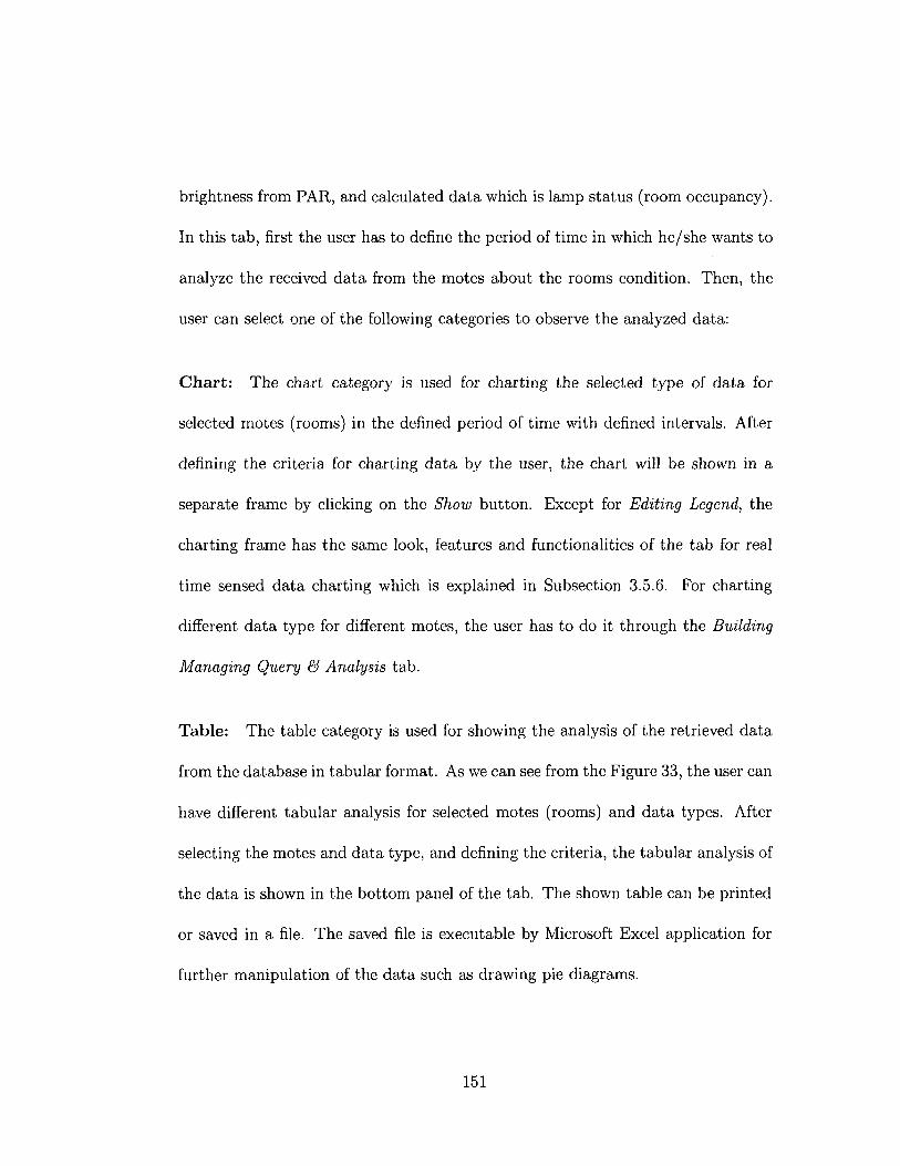
brightness from PAR, and calculated data which is lamp status (room occupancy).
In this tab, first the user has to define the period of time in which he/she wants to
analyze the received data from the motes about the rooms condition. Then, the
user can select one of the following categories to observe the analyzed data:
Chart: The chart category is used for charting the selected type of data for
selected motes (rooms) in the defined period of time with defined intervals. After
defining the criteria for charting data by the user, the chart will be shown in a
separate frame by clicking on the Show button. Except for Editing Legend, the
charting frame has the same look, features and functionalities of the tab for real
time sensed data charting which is explained in Subsection 3.5.6. For charting
different data type for different motes, the user has to do it through the Building
Managing Query & Analysis tab.
Table: The table category is used for showing the analysis of the retrieved data
from the database in tabular format. As we can see from the Figure 33, the user can
have different tabular analysis for selected motes (rooms) and data types. After
selecting the motes and data type, and defining the criteria, the tabular analysis of
the data is shown in the bottom panel of the tab. The shown table can be printed
or saved in a file. The saved file is executable by Microsoft Excel application for
further manipulation of the data such as drawing pie diagrams.
151

List: The list category is used for listing two sets of data. The first set is about
listing the rooms (motes) with defined range for average of selected data type
sensed during the defined period of time. The second set is the dates and times in
which the selected mote (room) sensed the selected data type in the defined range.
The list are shown in the bottom panel of this tab. The lists can also be printed
or saved in a file.
In Building Managing Query & Analysis tab, whenever the user wants to select
motes for analysis, he/she has to click on Select Motes (Rooms) button in the
appropriate category. After clicking on the button, the new frame titled Select
Motes (Rooms) is opened for mote selection which is shown in Figure 34. This
frame lets the user selects up to five motes (rooms) individually or all motes (rooms)
from the drop down menu. The drop down menus are filled automatically by
retrieving list of the motes (rooms) from the database. In addition, Building
Managing Query & Analysis tab has a message bar which informs the user about
the cause of failed execution of the queries if there is any. The messages are usually
for informing the user about selecting the wrong criteria, not selecting the right
category or forgetting to select the motes (rooms).
3.5.8 Data query and analysis for network administrating
The users responsible for administrating the wireless sensor network are interested
in retrieving the data from the database to analyze different aspects of the network
152

Select Motes(Rooms)
Mote(Room) 1:
Mote(Room) 2:
Mote(Room) 3;
Mote(Room) 4:
Mote(Room) 5:
All Motes(Rooms): 0
OK CANCEL
Figure 34: The graphical user interface for selecting motes (rooms) for data query and analysis.
such as the motes connectivity, the network's reliability and power usage of the
motes. The Network Administrating Query & Analysis tab (shown in Figure 35)
provides the interface for the user to query and analyze the data archived in the
database. In this tab, first, the user has to define the period of time in which
he/she wants to analyze the data. Then, the user can select one of two categories
(Chart or Table) for viewing analyzed data. The two categories are as follows:
Chart: The chart category is used for charting two types of data which are link
quality and power. For link quality data type, the user charts the quality of the
links from the selected motes to their neighbors in the defined period of time with
defined intervals. For power, the user charts the power of the selected motes in
defined period of time with defined intervals. The charts are shown in a separate
frame. The charting frame for both data types has the same look, features and
functionalities of the tab for real time link quality charting which is explained in
153

- ij/j
vmi •
r.-rfiO
inT,
File
O
ptio
ns
Rea
l tim
e To
polo
gy: i
Rea
l tim
e D
ata
Cha
rting
jj R
eal t
ime
Link
Qua
lity
Cha
rting
Bu
Hding
Man
agin
g Q
uery
& A
naly
sisj
Net
wor
Adm
inis
tratin
g Q
uery
Si A
nalys
is j
I To
: D
ate
Perio
d:
From
: :
08/0
9/25
,12:
00:0
0:00
0 {0
8/09
/27,
12:0
0:00
:000
O
Cha
rt
Mot
es(R
oom
s):
0 Ta
ble
Mot
es(R
oom
s):
Sele
ct M
otes
(Roo
ms)
Se
lect
Mot
es(R
oom
s)
Dat
a Ty
pe:
Inte
rval
:
Q
With
Ave
rage
Q
Mes
sage
s &
Lost
s C
ourt
with
its
Rat
io
Q
Pow
er U
sage
& T
ime
to F
ailu
re D
iffer
ence
s
Q
Aver
age
Pow
er U
sage
Q
Dis
tribu
tion
of S
elec
ted
Mot
e Pa
rent
s w
ith A
vera
ge L
ink
Qua
lity
0 D
istri
butio
n of
Sel
ecte
d M
ote
Chi
ldre
n w
ith A
vera
ge If
flk Q
ualit
y
Mes
sage
s: j
You
Can
See
Res
ult o
f Jus
t One
Mot
e Be
low
.
Ta
ble
Show
l|
Res
et
: Dat
e Fr
om
Dat
e To
Pe
riod
in D
ays
Perio
d in
Hou
rs
Child
ID o
f M
ote
8185
(...
Child
Roo
m#
Tota
l Rep
etiti
on
Dis
tribu
tion
Perc
enta
ge
Ave
rage
link
Qua
fity
j
iThu
Sep
25
12:0
0:00
ED
...
Sat
Sep
27 1
2:00
:00
EDT.
.. 2
48
8161
EV
8161
1
0.01
83
52.0
iT
hu S
ep 2
5 12
:00:
00 E
D...
Sa
t Se
p 27
12:
00:0
0 ED
T...
2 48
81
69
EV81
69
6 0.
1099
16
7.66
67
iThu
Sep
25
12:0
0:00
ED
...
Sat
5ep
27 1
2:00
:00
EDT.
.. 2
48
8173
EV
8173
52
D
.952
4 36
.576
9 IT
hu S
ep 2
5 12
:00:
00 E
D...
£a
t Se
p 27
12:
00:0
0 ED
T...
2 48
81
77
EV81
77
282
5.16
48
34.7
482
jThu
Sep
25
12:0
0:00
ED
...
[Sat
Sep
27
12:0
0:00
ED
T...
2 48
81
81
EV81
81
1399
8 73
.223
4 55
.035
8 jT
hu S
ep 2
5 12
:00:
00 E
D...
Sa
t Se
p 27
12:
00:0
0 ED
T...
2 48
81
87
EV81
87
1121
20
.531
1 35
.725
2
Figu
re 3
5: T
he g
raph
ical
use
r in
terf
ace
for
quer
ying
dat
abas
e an
d an
alyz
ing
retr
ieve
d da
ta b
y th
e us
ers
resp
onsi
ble
for
the
netw
ork
adm
inis
trat
ing

Subsection 3.5.6.
Table: The table category is used for showing the analysis of the retrieved data
from the database in tabular format. For analysis, the user has to set the period
of time, and then select the motes. Then, the user can select the desired type of
analysis. The table will be shown in the bottom panel after clicking on the Show
button. The tabular analysis can also be printed and saved as a file. Figure 35
shows different kinds of analysis that can be performed under table category.
In the Network Administrating Query & Analysis tab, whenever the user wants
to select motes for analysis, he/she has to click on Select Motes (Rooms) button
in appropriate category. The frame for selecting the motes (rooms) has the same
look and functionalities as the one in Building Managing Query & Analysis tab.
The Select Motes (Rooms) frame is shown in Figure 34. In addition, there is a
message bar in Network Administrating Query & Analysis tab which is used for
the same purpose as the one in Building Managing Query & Analysis tab.
Moreover, the generated charts and tables in Network Administrating Query &
Analysis tab are shown and explained in Chapter 4.
155

Chapter 4
Data collection and analysis
In this chapter, first, we describe the deployment process of automated building
monitoring system by wireless sensor network. Second, we analyze the system
robustness and correctness along with network reliability and life time. Then, we
explain the analysis of the collected data.
4.1 System deployment
We deployed and tested our system in the Engineering and Visual Arts (EV)
building of Concordia University. Figure 36 shows the floor map of the 8th floor
of the building; Rooms 9.101 and 9.105 in the 9th floor have been placed in the
left top corner in order to have all rooms in the same picture. In reality, these two
rooms are placed exactly over rooms 8.101 and 8.105 in the 8th floor.
We monitored 26 rooms in the 8th floor and 2 rooms in the 9th floor. We
156

9.1
01
0.1
05
• •
8.11
9
8.1
43
8.1
65
nn
nn
8.1
65
8 101
8.1
42
8.1
61
The
gate
way
mot
es
8.1
77
8.1
73
8.181
The
Sink
• 8.1
50
• 8.1
54
• 8.2
30
• 8.2
10
• 8.2
45
• 8.2
41
• 8.2
35
• 8.2
25
• 8.2
21
• 8.2
15
# R
epre
sent
s a
sens
or n
ode
Figu
re 3
6: F
loor
map

Figure 37: Tmote Sky mote (the 2$ coin is placed alongside to give an idea of the actual size of the mote)
programmed 31 Tmote Sky motes to form our wireless sensor network. Figure 37
shows one of the Tmote Sky motes that were used in our system. One of the motes
was used as the sink and was placed in room 8.161. The sink was connected by
the USB port to the PC on which the gateway/server was running. Twenty eight
of the motes were placed in the rooms of the 8th and 9th floor. Two of the motes
were used as the gateway motes in our wireless sensor network and were placed
in the hallway of the 8th floor. The gateway motes were used to keep the whole
network connected. Without using the gateway motes, the motes in top left of
the floor map, which are shown in Figure 36, were disconnected from rest of the
network due to the long distance they have from the nearest mote.
Each mote id was set according to the room number in which it has been placed
158

except the sink and gateway motes. For instance, the id of the mote placed in room
8.161 was set to 8161. The id of the sink was set to 0 and the id of the two gateway
motes were set to 1 and 2.
For avoiding interference between the motes radio frequency and WLAN al-
ready working in the building, the radio channel of the motes were set to 26 work-
ing at radio frequency of 2.480 kHz. The features and specifications of the motes'
radio transceiver are explained in Subsection 3.3.1. In addition, the power index of
all the motes was set to 10, which equals -8dBm. This transmission power enables
the motes to communicate with other motes at a distance of 8 to 10 meters. We
chose the lowest possible transmission power for the motes to enable the motes to
make reliable and robust multi-hop communication to the sink while considering
energy conservation.
Each mote (except the sink and gateways) was placed over a lamp frame in
its room, in such a way that the side of the board with sensors (not the battery
side) was facing the ceiling. Figure 38 shows the mote placed over the lamp frame
in room 8.161. As explained in Subsection 3.3.4, the mote's light sensors have to
be placed close to the lamp's light and away from the direct sunlight to be able
to sense the flickering of the light generated by the lamps. This is the reason for
the choice of the placement of motes. In addition, with this placement, readings
of the humidity and temperature sensors were accurate and reflected the exact
temperature and humidity in the rooms.
159

Figure 38: The placement of the mote over the lamps frame of room 8.161
160

We collected data and tested our system for 50 days (from October 1st, 12:01PM
to November 20th, 12:01PM). The analysis of the collected data and performance
of the system are explained in the rest of this chapter.
4.2 System analysis
Since there is no other automated building monitoring system using wireless sensor
network, we cannot validate our system by comparing to other existing tools or
research. However, we discuss the system correctness and robustness, and network
reliability and life time in subsequent subsections.
4.2.1 System correctness
We checked the correctness of the data in our system manually or by use of other
tools. For instance, for checking the correctness of reported temperature and
humidity readings by all motes in the network, we compared the reported readings
with manual readings taken using a La Crosse Technology thermometer in every
room at different times. Similarly, for checking the correctness of reported lamp
status, we checked the status of the lamps in all rooms at different times of the day.
The mentioned methods were used for checking the correctness of the reported data
during the collection period. Beside that, we checked and tested the correctness
of every sensor and reported readings individually before deploying the motes.
161

4.2.2 System robustness
During the 50 days of data collection, the gateway/server and end user applica-
tion ran in an uninterrupted fashion. The system successfully handled different
types of exceptions such as bad received messages and interrupted server/client
connection. The system can also detect intrusions and unexpected movement of
the motes in wireless sensor network. For intrusions, the end user application can
detect messages from unexpected motes and alerts the end user. For unexpected
movement of the motes, the end user application consults each mote's neighbor
list and informs the end user in case of any major change. However, these features
were not tested.
4.2.3 Network reliability
Each mote sends a message every 30 seconds to the end user in our system. There-
fore, the end user application is expected to receive 144,000 messages from each
mote and 4,464,000 messages in all during the 50 days of data collection. The
number of received messages increases with the generation of the messages by the
motes for alerting the end user, since the alerting messages are generated more
frequently (every 5 seconds) than regular messages. The cases where the system
generates messages for alerting the end user are explained in Subsection 3.3.3.
During the testing period, no critical situation happened in the building rooms.
Therefore, there were no alerting messages from the motes.
162

Figure 39 shows the ratio of successfully received and lost messages to the total
expected number of messages for each mote in the network during the 50 days of
data collection. From this figure, we can see that the loss ratio of all motes in 8th
floor is less than 5%. With such low loss ratio for our wireless sensor network, we
can conclude that this wireless sensor network is reasonably reliable for building
monitoring. Furthermore, we can see from the Figure 39 that the motes with id
9101 and 9102 in 9th floor have high loss ratio of more than 20%. The reason
is that the motes in 9th floor have links with low link quality to their neighbors
in 8th floor due to thick layer of cement and metal combined between the floors.
Therefore, it is not recommended to place the communicating motes in different
floors of the building.
Furthermore, with high ratio of successful message delivery, we can also con-
clude that the network was well-connected without loops during testing period.
However, we can analyze the connectivity of each mote to its neighbors by using
the information of the links and their quality from each mote to its neighbors. This
information is archived during the testing period in the link table in our database.
For instance, Figure 40 shows the connectivity statistics of mote 9101 during the
50 days of data collection. We can see that mote 9101 selected mote 9105 as its
parent about 56% of the time due to the good link quality to this neighbor. Also,
the mote 8109 has been selected as its parent just in 10% of the time due to its
bad link quality. Recall that lower the link quality indication is, better the actual
163

OS
? R
ecei
ved
Mes
sage
s •
Los
t M
essa
ges
S101
81
09 81
15 S1
19
8143
81
50
in
'XI
CO
00
> >
Ui
LU
8154
S1
61 81
65
at
CO
00
> >
ILl
8169
81
73 81
77
Mat
e id
and
ro
om
nu
mb
er
€Q
GO
CO
> >
> U
i LJ
LU
8181
81
85 81
87
8210
82
15
8230
82
35
8412
91
01
Figu
re 3
9: R
atio
of
succ
essf
ully
rec
eive
d an
d lo
st m
essa
ges
to t
otal
exp
ecte
d m
essa
ges
for
each
mot
e in
the
net
wor
k

One-hop neighbor motes distribution
H Average link quality
800 -s 700 • .a a
600 •a 500 500
9» 400 s re 300 c 200 s
—J 100
0 n EV8.101 EV8.105 EV8.109 EV9.105
8101 8105 8109 9105
O n e - h o p n e i g h b o r m o t e id and r o o m n u m b e r
Figure 40: One-hop neighbor motes distribution and average link quality of mote 9101 in room 9.101
link quality is. From the average link quality of mote 9101 to its neighbor motes in
Figure 40, we can conclude that the mote 9101 link quality to all of its neighbors
in 8th floor is very low and this caused the high ratio of the lost messages for mote
9101, which is shown in Figure 39. Furthermore, Figure 41 shows connectivity
statistics of mote 8210 in 8th floor during the 50 days of data collection. This
mote has good link quality to its neighbors and has less than 5% loss ratio. This
figure shows that worst link qaulity of mote 8210, which is to mote 8187, has al-
most the same average link quality as best link quality of mote 9101 which is to
mote 9105.
Finally, the delay and processing time of receiving messages from the motes
to the end user application is very low in this system. The interval of generating
messages by the motes in the system is 30 seconds and the average interval time of
the received messages from all motes during the testing period was 30.5 seconds.
165

One-hop neighbor motes distribution
8187 EV8.187
8230 EV8.230
13%
SIM FV8134 /
S 3 « • ""
D Average link quality
120
J 10° 80 .8 •o 60
40
20
S*50 u -
EV8150 29ft
EV8.187 EV8.230 EV8.150 EV8.154 EV8150 29ft
8187 8230 8150 8154
One-hop neighbor mote id and room number
Figure 41: One-hop neighbor motes distribution and average link quality of mote 8210 in room 8.210
4.2.4 Network lifetime
As explained in Subsection 3.3.6, a duty cycle of 5% would enable motes to be
functional for 107 days. At the end of 50 days, therefore we expect the motes to
have used up to 50% of their power source. Figure 42 shows the remained and
used power of all motes in our network at the end of the 50 days of data collection.
As we can see from this figure, most of the motes except those on 9th floor have
used about half of their power source during 50 days, which is about half of the
expected life time of the motes. This validates the calculation of the lifetime and
the correct functionality of the motes at the specified duty cycle.
The reason that the motes in 9th floor were consuming more power than the
other motes was due to their bad connectivity to the motes in 8th floor. The
poor connectivity caused these motes to not receive the synchronization beacon on
time. Therefore, after their synchronization had been timed out, they kept their
166

a R
emai
ned
pow
er
• U
sed
pow
er
Figu
re 4
2: R
emai
ned
and
used
pow
er s
ourc
e of
all
mot
es

radio transceiver on in high power duty cycle (100% duty cycle) to receive the new
synchronization beacon, thereby consuming more power.
4.3 Data analysis
During the 50 days of data collection, we collected the lamp status (room occu-
pancy), temperature, humidity and brightness of the rooms. In this section, we
analyze the collected data from all motes except the sink and the gateways.
The building in which we have tested our system has an automatic system for
turning off the cooling, heating and ventilation system as well as the lamps of the
rooms when there is no motion detected in the room. In the other words, when
someone steps in the room the lamp, heating or cooling, and ventilation of the
room turns on automatically based on the signal from the motion detector in the
room. When no motion is detected for the period of 15 minutes, the lamps and
other systems get turned off to conserve energy.
4.3.1 Lamp status (room occupancy) data analysis
Figure 43 shows the lamp status (room occupancy) statistics of all rooms during
the testing period. From this figure, we can see that some rooms such as 8.412
and 9.101 were rarely used. In addition, we may conclude from Figure 43 that
room 8.173 and 8.101 were occupied most of the time. However, we checked these
rooms and we figured out that while room 8.101 is mostly occupied, the room
168

8.173 motion detector does not appear to shut off the lamps in this room, which
are always on, unless manually turned off. Therefore, the correct occupancy of
the room 8.173 cannot be deduced from our data. Also in Subsection 4.3.3, we
explain how the analysis of the temperature and humidity data with lamp status
can determine whether or not the motion detector in each room is functioning
correctly.
4.3.2 Brightness data analysis
With the analysis of Brightness data, we can check whether each office has the
necessary light provided by the lamps. In addition, we can figure out about the
lamps that are not functioning any more by detecting changes in brightness level
over time. Figure 44 shows the minimum and maximum brightness in all rooms
when the lamps are on. From this figure, we can see that the minimum brightness in
rooms 9.105 and 8.241 during the testing period was less than the required standard
brightness for office work. The standard required brightness in each room for office
work is at least 500 lx. However, the maximum values in both rooms were high
enough to meet the standard. Therefore, we checked the lamps of these rooms and
we figured out that one lamp in each room had been malfunctioning. In addition,
we can see from this figure that the maximum of some rooms such as 8.101 and
8.105 are very high due to the daylight in these rooms through their windows.
Figure 45 shows the brightness level from 8:25AM to 2:49PM of October 2nd in
169

Figu
re 4
3: L
amp
stat
us (
room
occ
upan
cy)
stat
istic
s du
ring
the
50
days
of
test
ing
peri
od

• M
inim
um b
righ
tnes
s(lx
) •
Max
imum
br
ight
ness
(lx)
2500
1 q
en
«H 1
2 I in
•H 1
in 1
8154
82
10
8119
S4
12
8115
Figu
re 4
4: M
inim
um a
nd m
axim
um o
f th
e br
ight
ness
in
all
room
s w
hen
the
lam
ps a
re o
n

1600 1400
a 1200 Hf 1000 I 800
600 400 200
0
.a CO
Ln IN 66 f N O
o »-l
oJ o
rn in oi rvi in TH m o in m (6 <ji rn o CO CO oi fN in in o o o ^ ^ o o o «-l I - l . H
o o o
m rH ? » rn in rn o oi in m 0) IN IN o o
00
o o o o
CD in IN ID CO IN IN rn in <ri 00
(N IN O O
O O in <H
o m
00 00 oi N m ffl o Ul ID 1/1 N " o m in m IJ3 o ID m m m irt (D in ID IN
in pi lii IN r-l T-l rH
Ch in pn m o IJD (N
oi in O ID M m o <7) IN in in o m in ro m
m in o
fN fN fN IN O O O O
O IN m r
IN IN IN IN fN rN fN O O O O O O O T H O O O O O O O O O O O O O O O O O O O
OOOOOOTOTOWOOOaOOOOOOOOOOOOOOOOOOOOOOMOO o o p o o o o o o o o o o o o o o o o
Figure 45: Brightness level in room 8.101 on October 2nd from 8:24AM to 2:49PM. Note that lamp status was off during this period.
room 8.101. The lamp status in this period is off. We can see from this figure that
there is more than enough light in the room due to the daylight for office work,
therefore turning the lamps on in the room automatically by the motion detector
causes unnecessary energy consumption. This points to a limitation of using a
motion detector exclusively as a method for energy conservation.
4.3.3 Temperature and humidity data analysis
Figure 46 shows the temperature and humidity changes in room 8.165 during one
day. In this figure, the lamps are off when the lamp status curve is zero and
the lamps are on when the lamp status curve is 70. When the motion detector
detects any movement in the room, the lamps, heating and ventilation system are
172

turned on. When the heating and ventilation systems are off, in cooler weather,
the temperature drops and the humidity rises in rooms.
By combining the lamp status data with the temperature and humidity data, we
can analyze the functionality of the ventilation and heating systems. In addition,
we can analyze the correctness of the lamp status data in relation to the room
occupancy of the room. For instance, as we mentioned in Section 4.3.1, the motion
detector in room 8.173 is not functional. Figure 47 shows the detailed temperature,
humidity and lamp status data collected for room 8.173 during one day of the
testing period. From this figure, we can see that even when the lamp status
was always on, the temperature and humidity are adjusting due to the motions
detected in the room. Therefore, the problem in this room is not related to the
motion detector, but the problem is that the lamp switch is not reacting to the
motion detector signals.
Figure 48 shows the minimum, maximum and average of temperature in all
rooms when the ventilation and heating systems were on (when the lamps are on)
during the 50 days of testing. Figure 49 shows the distribution of the temperature
values of room 8.165 during the testing period when the ventilation and heating
system were on. We can also have the same figures for humidity.
173

lam
p st
atus
(70
=on. 0
=of
f) --
Tem
perr
ture
pC)
Mum
idity
(%)
70
60
50
40
30
20
10
70
60
50
40
30
20
10
70
60
50
40
30
20
10
70
60
50
40
30
20
10
V
70
60
50
40
30
20
10
- .
70
60
50
40
30
20
10
~
70
60
50
40
30
20
10
70
60
50
40
30
20
10 c
08/10/02,0:00:05:125 08/10/02.0:15:40:140 08/10/02,0:32:39:015 08/10/02,0:49:41:765 08/10/02,1:07:56:937 08/10/02,1:48:20:703 08/10/02,2:33:21:500 08/10/02,2:52:36:562 08/10/02,3:09:21:484 08/10/02.3:25:32:750 08/10/02.3:42:51:687 08/10/02,3:57:58:671 08/10/02,4:14:27:906 08/10/02,4:29:03:734 08/10/02.4:44:26:796 08/10/02,5:00:53:968 08/10/02.5 16 23.4*8 08/10/02,5:31:53:093 08/10/02,5:51:47:234 08/10/02.6:18:49:765 08/10/02,6:41:09:953 08/10/02,6:58:13:500 08/10/02,7:18:15:906 08/10/02,7:41:08:078 08/10/02,8:04:22:234 08/10/02,8:27:51:453 08/10/02,8:46:25:984 08/10/02,9:01:42:343 08/10/02,9:19:52:906 08/10/02,9:36:45:437 08/10/02,9:54:02:046
08/10/02,10:23:39:125 08/10/02,10:49:18:890 08/10/02,11:13:51:187 08/10/02,11:28:43:468 08/10/02,11:45:25:734 08/10/02,12:03:34:000 08/10/02,12:25:14:328 08/10/02,12:46:52:890 08/10/02,13:12:49:343 08/10/02,13:29:15:453 08/10/02,13:44:43:562 08/10/02,14:01:14:765 08/10/02,14:18:14:921. 08/10/02,14:34:45:390 08/10/02,14:51:13:671 08/10/02,15:06:50:656 08/10/02,15:22:19:609 08/10/02,15:39:02:187 08/10/02,15:54:44:453 08/10/02,16:13:45:046 08/10/02,16:28:45:390 08/10/02,16:44:25:609 08/10/02,17:02:14:078 08/10/02,17:19:44:625 08/10/02,17:39:44:968 08/10/02,17:55:15:343 08/10/02,18:11:45:671 08/10/02,18:27:15:953 08/10/02,18:42:44:703 08/10/02,19:00:49:015 08/10/02,19:19:45:281 08/10/02,19:35:21:718 08/10/02,19:51:44:171 08/10/02,20:06:16:28,1 08/10/02,20:23:44:S62 08/10/02,20:39:45:203 08/10/02,20:55:15:687 08/10/02,21:10:45:812 08/10/02,21:25:46:203 08/10/02,21:43:46:609 08/10/02,22:01:15:171 08/10/02,22:16:46:015 08/10/02,22:32:16:390 08/10/02,22:49:17:000 03/10/02.23:04:41:343 08/10/02,23:19:15:81.2 08/10/02,23:33:46:359 08/10/02,23:49:17:093
Figu
re 4
6: T
empe
ratu
re,
hum
idit
y an
d la
mp
stat
us c
hang
es i
n ro
om 8
.165
dur
ing
one
day
of th
e te
stin
g pe
riod

- La
mp
stat
us (
70=o
n. O
=off)
Te
mpe
ratu
re(sC
) -H
umid
ity(%
)
llilll
llllS
lIlS
SSill
lillll
llSSl
iililS
SlilS
IIilf
iillll
lllfS
iliiS
Iifll
llilii
li "
••-• "
"
"i s
r g
g s
S a
a S
s s
S s
S s
a S
a s
s r
g s
a 5
I a
gis
ssss
^
„- j
„- .
Ill
llll
llll
llll
llll
llll
llll
llll
llll
llll
llll
^ rtS
rifiS
nS^i
iiiiii
SiSN
SNi:
3 2
2 3
3 3
2 2
5 2
2 2
2 2
3 2
2 2
2 3
2:
Figu
re 4
7: T
empe
ratu
re,
hum
idit
y an
d la
mp
stat
us c
hang
es i
n ro
om 8
.173
dur
ing
one
day
of t
he t
esti
ng p
erio
d
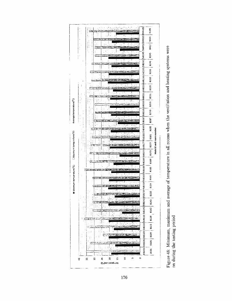
OS
I M
inim
um t
empe
ratu
re^C
! O
Max
imum
tem
pera
ture
(sC!
Ave
rage
tem
pera
ture
(°C
]
BL™
,
EVS2
35 E
V82
41 E
VB
245
EV84
12 E
V91
01 E
V91
05
S235
82
41
8245
84
12
9101
91
05
Mot
e id
and
roo
m n
umbe
r
Figu
re 4
8: M
inim
um,
max
imum
and
ave
rage
of
tem
pera
ture
in
all r
oom
s w
hen
the
vent
ilatio
n an
d he
atin
g sy
stem
s w
ere
on d
urin
g th
e te
stin
g pe
riod

Figure 49: Distribution of the temperature values in room 8.165 when the venti-lation and heating systems were on during the testing period
4.4 Discussion
In this section, we discuss the challenges involved in implementing the system as
well as the extent and the limitations of the information obtained.
The first challenge in implementation is extending the life time of the wireless
sensor network. As we explained in Subsection 4.2.4, motes are operational for
about 100 days if they are in good communication range of each other and they
are using a 5% duty cycle. However, it is challenging to increase the life time of
the motes by using lower duty cycle and still fullfil the end user requirement such
as having the most up-to-date data. The lifetime of nodes is also affected by the
problem of poor connectivity as explained below.
177

The second challenge is connectivity between the motes in different floors. As
we explained in Subsection 4.2.3, motes in different floors cannot communicate
with each other due to the concrete barriers between the floors. Therefore, the
network is not well-connected between the floors. For this problem, we propose
the solution of placing one sink in each floor and making separate collection trees
in each floor rooted at the sink placed in the same floor. In other words, one
mote is placed in each room of the building. Each mote in a floor has a unique
address (id). Two motes can have the same id as long as they are on two different
floors. All motes in each floor have the same group id which is programmed in the
motes at the same time with their ids. The group id for each floor is unique. This
makes the motes form separate networks in different floors. Therefore, when there
are many motes in the whole building and the motes in different floors can not
communicate to each other with good link quality, the mentioned way of separation
of the motes between each floor can make better quality of service and also aid
energy conservation, which can further increases the lifetime of the motes.
The third challenge is massive data processing by the gateway/server and the
end user application. We have used a commercial database and a multi-threading
approach to meet this challenge. The massive data processing can also be solved
by using hardware with higher capabilities in terms of memory and computation or
by using different programming techniques such as direct hardware access instead
of using operating system APIs.
178

There are different types of information that have been obtained from the
deployment of our system. Watching the indoor environment condition of the
building is the information that provides the end user with real time status of the
room climate and lamp status such as the one shown in Figure 48. As Figures
49 and 44 show, the end user can also monitor and optimize the ventilation and
lighting system by having the information extracted from the periodic report of
climate condition and lamp status of each room. We have considered lamp status
of each room as an approximation to room occupancy in this thesis: a room is
occupied when the lamp is on and it is unoccupied when the lamp is off. However,
this is not always true such as in room 8.173 as was explained in Subsection 4.3.1.
Furthermore, the end user can also determine the performance of already existing
building monitoring systems or diagnose individual building facility performance
remotely by combining the data reported for different metrics such as humidity and
temperature to derive new information as explained in Subsection 4.3.3. Finally,
studying the possible energy conservation methods can be performed by the end
user such as turning the lights on/off centrally for the rooms with enough light
provided from daylight as shown in Figure 45.
179

Chapter 5
Conclusion and recommendations
for future work
In this thesis, we proposed and developed a system for building monitoring using
wireless sensor network technology. Even though during the last decade, there have
been several research projects that have led to some improvements in different ar-
eas (subfields) of wireless sensor networks, there has not been enough focus on the
application layer of this technology in building monitoring. In this thesis, we devel-
oped an automated building monitoring system using a wireless sensor network for
monitoring climate, brightness and lamp status of the rooms in the building. By
using the status of the lamps in the rooms, we monitor the occupancy of the rooms
as well. Our system consists of three main subsystems: wireless sensor network,
gateway/server and end user application. The wireless sensor network reports the
180

collected data for temperature, humidity and brightness and the calculated data,
which is lamp status (room occupancy) to the sink while considering energy con-
servation by using low power duty cycle. The gateway/server forwards the received
data from the sink to the end user application that is connected to it. In addition,
the gateway/server archives the received data in a database for later retrieval and
analysis. The end user application visualizes the network connectivity. It provides
tools to view and search a mote's information. It also provides charts for analyzing
the information based on the received data for two categories of users, namely the
building manager and the network administrator. The application interprets the
data from the database in order to analyze the building climate, room occupancy
and brightness, and functionality of the heating, cooling and ventilation system of
the building.
We are optimistic that this system provides a much simpler and more flexible
system design than old-fashioned wired building monitoring systems. Our system
allows for faster and easier installations at a lower cost and with fewer constraints
associated with maintenance. Finally, our system provides more accurate and ro-
bust analysis of the information about building climate conditions and controlling
systems as well as room occupancy. As explained in Section 4.4, the most impor-
tant challenges encountered system implementation were extending the life time
of the wireless sensor network, connectivity between the motes in different floors,
and massive data processing by the gateway/server and end user application.
181

For future work, we believe that the system can be complemented by improv-
ing the routing algorithm to have guaranteed delivery for alert messages, having a
localization algorithm in the network to track objects or staff in the building, ag-
gregating data for situations with more than one mote in one room, implementing
a dissemination algorithm for commanding and reprogramming the motes over the
air in the network, decreasing the power consumption of the mote, making a sys-
tem model for building monitoring applications, analyzing data automatically, and
controlling the building heating, cooling, ventilation and lighting systems locally
by motes.
182

Bibliography
[1] Petzl reference system for lighting performance.
http://en.petzl.com/petzl/frontoff ice/Lampes/static/referentiel
/present_referentiel_en.j sp
[2] RFID Tags and Chips: Changing the World for Less Than the Price of a Cup
of Coffee. In-Stat/MDR Report, Jan 2005.
[3] Kemal Akkaya and Mohamed Younis. A survey on routing protocols for wire-
less sensor networks. Elsevier Ad Hoc Network Journal, 3:325-349, 2005.
[4] I. F. Akyildiz, W. Su., Y. Sankarasubramaniam, and E. Cayirci. Wireless
sensor networks: A survey. Computer Networks (Elsevier) Journal, pages
393-422, 2002.
[5] J. N. Al-Karaki and A. E. Kamal. Routing techniques in wireless sensor
networks: a survey. IEEE Wireless Communications, 11(6):6—28, 2004.
[6] Refrigerating American Society of Heating and Air-Conditioning Engineers,
http://www.ashrae.org
183

[7] T Antoine-Santoni, JF Santucci, E De Gentili, and B Costa. Using wireless
sensor network for wildfire detection, an discrete event approach of an eviron-
mental monitoring tool. In Proceedings of the First international Symposium
on Environment Identities and Mediterranean Area, ISEIM 2006, pages 115—
120, July 2006.
[8] Reliable Arbor: A robust and platform independent collection service,
ht tp : / /www.Stanford .edu /c lass /cs244e /papers /c tp .pdf
[9] Canadian Standards Association, http://www.csa.ca/
[10] IEEE Standards Association, http://standards.ieee.org/
[11] Grady Booch, Ivar Jacobson, and Jim Rumbaugh. OMG Unified Modeling
Language Specification. Rational software corporation, March 2000.
[12] David Braginsky and D. Estrin. Rumor routing algorithm for sensor networks.
In Proceedings of the First Workshop on Sensor Networks and Applications
(WSNA), pages 22-31, 2002.
[13] Rachel Cardell-oliver, Keith Smettem, Mark Kranz, and Kevin Mayer. Field
testing a wireless sensor network for reactive environmental monitoring. In
Proceedings of the International Conference on Intelligent Sensors, Sensor
Networks and Information Processing, pages 14-17, 2004.
184
[14] A. Chandrakasan, R. Amirtharajah, S. Cho, J. Goodman, G. Konduri, J. Ku-
lik, W. Rabiner, and A. Wang. Design considerations for distributed micro-
sensor systems. In Proceedings of the IEEE 1999 Custom Integrated Circuits
Conference, page 279286, 1999.
[15] M. Chu, H. Haussecker, and F. Zhao. Scalable information-driven sensor
querying and routing for ad hoc heterogeneous sensor networks. The Interna-
tional Journal of High Performance Computing Applications, 2002.
[16] Boomerang Software documentation.
h t t p : / / docs . t i nyos .ne t / i ndex .php /Boomerang /
[17] e-SENSE website (Scenarios and audio visual concepts), 2006.
h t t p : / / w w w . i s t - e s e n s e . o r g
[18] D Estrin, L Girod, G Pottie, and M. Srivastava. Instrumenting the world with
wireless sensor networks. In Proceedings of the International Conference on
Acoustics, Speech and Signal Processing (ICASSP 2001), 2001.
[19] D Estrin, R Govindan, J Heidemann, and S Kumar. Next century chal-
lenges: scalable coordination in sensor networks. In Proceedings of the ACM
MobiCom 99, 1999.
[20] AA alkaline battery datasheet Eveready. h t t p : / / d a t a . e n e r g i z e r . c o m
185

[21] C. Federspiel, E. Arens, D. Auslander, C. Lin, S. Tang, and D. Wang. Xyz
on a chip: Integrated wireless sensor networks for the control of the indoor
environment in buildings.
[22] Saurabh Ganeriwal, Ram Kumar, and Mani B. Srivastava. Timing-sync pro-
tocol for sensor networks. In Proceedings of the SenSysOS, pages 138-149.
ACM Press, 2003.
[23] David Gay, Philip Levis, Robert von Behren, Matt Welsh, Eric Brewer, and
David Culler. The nesc language: A holistic approach to networked embedded
systems. In Proceedings of the ACM SIGPLAN 2003 conference on Program-
ming language design and implementation, pages 1-11, New York, NY, USA,
2003. ACM.
[24] Ramesh Govindan and Deborah Estrin. Directed diffusion: A scalable and
robust communication paradigm for sensor networks. In Proceedings of the
ACM International Conference on Mobile Computing and Networking (MO-
BICOM'OO, 2000.
[25] J. V. Greunen and J. Rabaey. Lightweight time synchronization for sensor
networks. In Proceedings of the WSNA03, 2003.
[26] Piyush Gupta, Student Member, and P. R. Kumar. The capacity of wireless
networks. IEEE Transactions on Information Theory, 46:388-404, 2000.
186

[27] J.A. Gutierrez, M. Naeve, E. Callaway, M. Bourgeois, V. Mitter, and B. Heile.
Ieee 802.15.4: a developing standard for low-power low-cost wireless personal
area networks. Network, IEEE, 15(5):12-19, Sep/Oct 2001.
[28] S. Hadim and N. Mohamed. Middleware: Challenges and approaches for
wireless sensor networks. Distributed Systems Online, IEEE, 7(3), March
2006.
[29] Thomas Haenselmann. SensorNetwork. GFDL Wireless Sensor Network text-
book, April 2006. Downloadable from
ht tp: / /www.informat ik .uni-mannheim.de/~haensel /sn_book/
[30] S. M. Hedetniemi, S. T. Hedetniemi, and A. L. Liestman. A survey of gossiping
and broadcasting in communication networks. Networks, pages 319-349, 1988.
[31] Wendi Rabiner Heinzelman, Anantha Ch, and Hari Balakrishnan. Energy-
efficient communication protocol for wireless microsensor networks. In Pro-
ceedings of the HICSS 00, Maui, pages 3005-3014, 2000.
[32] Jason Hill, Robert Szewczyk, Alec Woo, Seth Hollar, David Culler, and
Kristofer Pister. System architecture directions for networked sensors. SIG-
PLAN Not., 35(11):93-104, 2000.
[33] I. Howitt and J.A. Gutierrez. Ieee 802.15.4 low rate - wireless personal area
network coexistence issues. Wireless Communications and Networking, 2003.
WCNC 2003. 2003 IEEE, 3:1481-1486 vol.3, March 2003.

[34] CA In-Stat, San Jose, h t tp : / /www. in -s ta t . com
[35] Xilinx Inc. h t tp : / /www.xi l inx .com/
[36] MotelV incorporation website, http://www.moteiv.com
[37] Technology research center of Intel Corporation.
h t t p : / / t e c h r e s e a r c h . i n t e l . c o m / a r t i c l e s / E x p l o r a t o r y / 1 5 0 1 . h t m
[38] Sun Microsystems J2SE: Java Platform, Standard Edition,
h t t p : / / j ava .sun.com/j 2 s e / l . 4 . 2 /
[39] Bhaskar Krishnamachari, Deborah Estrin, and Stephen Wicker. Modelling
data-centric routing in wireless sensor networks. In Proceedings of the IEEE
INFOCOM, 2002.
[40] Joanna Kulik, Wendi Rabiner, and Hari Balakrishnan. Adaptive protocols for
information dissemination in wireless sensor networks. In Proceedings of the
5th Annual ACM/IEEE International Conference on Mobile Computing and
Networking (MobiCom99), pages 174-185, 1999.
[41] Sunil Kulkarni, Aravind Iyer, and Catherine Rosenberg. An address-light, in-
tegrated mac and routing protocol for wireless sensor networks. In Proceedings
of the IEEE/ACM Transactions on Networking.
[42] Philip Levis, Neil Patel, David Culler, and Scott Shenker. Trickle: a self-
regulating algorithm for code propagation and maintenance in wireless sensor
188

networks. In NSDI'04'- Proceedings of the 1st conference on Symposium on
Networked Systems Design and Implementation, pages 2-2, Berkeley, CA,
USA, 2004. USENIX Association.
[43] Li Li and Joseph Y. Halpern. Minimum energy mobile wireless networks revis-
ited. In Proceedings of the IEEE International Conference on Communications
(ICC, pages 278-283, 2001.
[44] Yingshu Li, My T Thai, and Weili Wu. Wireless Sensor Networks and Appli-
cations. Springer, 2008.
[45] Chunhung Richard Lin and Mario Gerla. Adaptive clustering for mobile wire-
less networks. IEEE Journal on Selected Areas in Communications, 15:1265-
1275, 1997.
[46] S. Lindsey and C. Raghavendra. Pegasis: Power-efficient gathering in sensor
information systems. In Proceedings of the IEEE Aerospace Conference, pages
9-16, 2002.
[47] Automated Buildings On line and web resource magazine website,
http://www.Automatedbuildings.com
[48] A. Manjeshwar and D. P. Agarwal. Teen: a routing protocol for enhanced effi-
ciency in wireless sensor networks. In 1st International Workshop on Parallel
and Distributed Computing Issues in Wireless Networks and Mobile Comput-
ing, 2001.
189
[49] A. Manjeshwar and D. P. Agarwal. Apteen: A hybrid protocol for efficient
routing and comprehensive information retrieval in wireless sensor networks.
In Proceedings of the International Parallel and Distributed Processing Sym-
posium, IPDPS, pages 195-202, 2002.
[50] Vivek Mhatre and Catherine Rosenberg. Design guidelines for wireless sensor
networks: communication, clustering and aggregation. Ad Hoc Networks,
2:45-63, 2004.
[51] Vivek Mhatre, Catherine Rosenberg, Daniel Kofman, Ravi Mazumdar, and
Ness Shroff. Design of surveillance sensor grids with a lifetime constraint.
In Proceedings of the First European Workshop on Wireless Sensor Networks
(EWSN 2004, pages 263-275, 2004.
[52] PA Mobility Technologies, Wayne, www.mobilitytechnologies.com/ntdc/
[53] NetsyncC component Moteiv Corporation.
http://tinyos.cvs.sourceforge.net/viewvc/tinyos/tinyos-1.x
/contrib/moteiv/
[54] TinyOS MultiHopLQI, 2004.
http://www.tinyos.net/tinyos-1.x/tos/lib/MultiHopLQI
[55] Sun Microsystems MySQL, h t t p : //www. mysql. com
190

[56] nesC: A Programming Language for Deeply Networked Systems,
h t t p : / / n e s c c . s o u r c e f o r g e . n e t
[57] CNET Network, h t t p : //www. cne t . com
[58] IEEE 1451 Family of Smart Transducer Interface Standards, October 2006.
h t t p : / / g r o u p e r . i e e e . o r g / g r o u p s / 1 4 5 1 / 0 / b o d y
°/020franie_f iles/Familyof-1451_handout .htm
[59] National Institute of Standards and Technology Guide to SI Units,
h t t p : / / phys i c s . n i s t . gov /Pubs /SP811 / sec09 .h tml
[60] TinyOS: An open-source operating system designed for wireless embed-
ded sensor networks, h t tp : / /www. t inyos .ne t
[61] Hamamatsu Corporation photodiodes datasheet,
http://www.hamamatsu.com
[62] J Polastre, R Szewczyk, C Sharp, and D Culler. The mote revolution: Low
power wireless sensor network devices. In Proceedings of the Hot Chips 16: A
Symposium on High Performance Chips, 2005.
[63] Joseph Polastre, Jonathan Hui, Philip Levis, Jerry Zhao, David Culler, Scott
Shenker, and Ion Stoica. A unifying link abstraction for wireless sensor net-
works. In SenSys '05: Proceedings of the 3rd international conference on Em-
bedded networked sensor systems, pages 76-89, New York, NY, USA, 2005.
191

ACM.
[64] Glacsweb project website, http: //www. envisense. org
[65] CA Rockwell Scientific, Thousand Oaks, http://www.rsc.rockwell.com
[66] Volkan Rodoplu, Student Member, and Teresa H. Meng. Minimum energy mo-
bile wireless networks. IEEE Journal on Selected Areas in Communications,
pages 1333-1344, 1999.
[67] K. Romer and F. Mattern. The design space of wireless sensor networks.
Wireless Communications, IEEE, 11(6):54-61, Dec. 2004.
[68] Narayanan Sadagopan, Bhaskar Krishnamachari, and Ahmed Helmy. The
acquire mechanism for efficient querying in sensor networks. In Proceedings
of the SNPA, pages 149-155, 2003.
[69] Paul Schlyter. Radiometry and photometry in astronomy faq.
[70] Curt Schurgers and Mani B. Srivastava. Energy efficient routing in wireless
sensor networks. In Proceedings of the MILCOM Proceedings on Communica-
tions for Network-Centric Operations: Creating the Information Force, pages
357-361, 2001.
[71] John C. Scott. Applications of telecommunications and information technol-
ogy for humanitarian health initiatives. In Proceedings of the PACMEDTEK
192

'98: Proceedings of the Symposium on Pacific Medical Technology, page 197,
Washington, DC, USA, 1998. IEEE Computer Society.
[72] SHTlx Sensirion sensor datasheet. h t tp : / /www.sensi r ion.com
[73] University of CaliforniaDavis Sensor Network Applications, Computer
Science Instructional Facility.
h t t p : / / w w w . c s i f . c s . u c d a v i s . e d u / ~ y i c k / s e n s o r / S e n s o r a p p l i c a t i o n . h t m
[74] R. C. Shah and J. Rabaey. Energy aware routing for low energy ad hoc
sensor networks. In Proceedings of the IEEE Wireless Communications and
Networking Conference (WCNC), pages 17-21, 2002.
[75] Sanjay Shakkottai, R. Srikant, and N. Shroff. Unreliable sensor grids: Cover-
age, connectivity and diameter. In Proceedings of the IEEE INFOCOM, pages
1073-1083, 2003.
[76] Eugene Shih, Seong hwan Cho, Nathan Ickes, Rex Min, and Amit Sinha.
Physical layer driven protocol and algorithm design for energy-efficient wire-
less sensor networks. In Proceedings of the Seventh Annual ACM Conference
on Mobile Computing and Networking (ACM MOBICOMOl), pages 272-287,
2001.
[77] Siemens, h t tp : / /www.bui ld ingtechnologies .usa . s iemens .com
193

[78] E. Siuonson and N. Enzer. Measurement of fusion frequency of flicker as a
test for fatigue of the central nervous system. Observations on laboratory
technicians and office workers industr. Hyg., 1941.
[79] Red Hat Software, h t tp : / /www.redhat .com/sof tware/cygwin/
[80] J. A. Stankovic, Q. Cao, T. Doan, L. Fang, Z. He, R. Kiran, S. Lin, S. Son,
R. Stoleru, and A. Wood. Wireless sensor networks for in-home healthcare:
Potential and challenges. In Proceedings of the HCMDSS, pages 2-3, 2005.
[81] Robert Szewczyk, Eric Osterweil, Joseph Polastre, Michael Hamilton, Alan
Mainwaring, and Deborah Estrin. Habitat monitoring with sensor networks.
Commun. ACM, 47(6):34-40, 2004.
[82] Quantifying Network Visibility.
h t t p : / / s i n g . S t a n f o r d . e d u / s r i k a n k / n t w r k v i s i b i l i t y . p d f
[83] Chipcon website, h t t p : //www. chipcon. com
[84] The Embedded Systems Website, h t tp : / /www.microcont ro l le r .com/
[85] Geoffrey Werner-Allen, Jeff Johnson, Mario Ruiz, Jonathan Lees, and Matt
Welsh. Monitoring volcanic eruptions with a wireless sensor network. In
Proceedings of the Second European Workshop on Wireless Sensor Networks
(EWSN05, 2005.
194

[86] J. Wilson, V. Bhargava, A. Redfern, and P. Wright. A wireless sensor net-
work and incident command interface for urban firefighting. In Proceedings of
the Fourth Annual International Conference on Mobile and Ubiquitous Sys-
tems: Networking & Services: MobiQuitous 2007, pages 1-7. Digital Object
Identifier, 2007.
[87] J. Wilson and P. Wright. Design of monocular head-mounted dis-
plays, with a case study on fire-fighting. In Proceedings of the Insti-
tution of Mechanical Engineers Part C-Journal of Mechanical Engineer-
ing Science, pages 1729-1743. Professional Engineering Publishing, 2007.
http://journals.pepublishing.com/content/119771.
[88] Alec Woo, Terence Tong, and David Culler. Taming the underlying challenges
of reliable multihop routing in sensor networks. In proceedings of the SenSys
'03, pages 14-27. ACM Press, 2003.
[89] Ya Xu, John Heidemann, and Deborah Estrin. Geography-informed energy
conservation for ad hoc routing. In Proceedings of the 7th annual international
conference on Mobile computing and networking, pages 70-84, New York, NY,
USA, 2001. ACM.
[90] Ya Xu, John Heidemann, and Deborah Estrin. Geography-informed en-
ergy conservation for ad hoc routing. In Proceedings of the 7th Annual
195

ACM/IEEE International Conference on Mobile Computing and Networking
(MobiComOl), pages 70-84, 2001.
[91] Yong Yao and Johannes Gehrke. The cougar approach to in-network query
processing in sensor networks. SIGMOD Record, 31:2002, 2002.
[92] Fan Ye, Alvin Chen, S. Liu, and L. Zhang. A scalable solution to minimum
cost forwarding in large sensor networks. In Proceedings of the tenth Inter-
national Conference on Computer Communications and Networks (ICCCN),
pages 304-309, 2001.
[93] Wei Ye, John Heidemann, and Deborah Estrin. An energy-efficient mac pro-
tocol for wireless sensor networks. In Proceedings of the IEEE INFOCOM,
pages 1567-1576, 2002.
[94] Feng Zhao and Leonidas Guibas. Wireless Sensor Networks: An Information
Processing Approach (The Morgan Kaufmann Series in Networking). Morgan
Kaufmann, July 2004.
196

Appendix A
Installation guide
The automated building monitoring system using wireless sensor network consists
of three subsystem which are wireless sensor network, the gateway/server and the
end user application. For running the system, first the code has to be compiled and
installed into the wireless sensor hardwares (motes). Second, the gateway/server
has to be run while the sink is connected to the USB port of the computer and
the computer is connected to Internet. Then, the end user application can be run
to receive data from the gateway/server.
In order to compile and install the code on the wireless sensor hardware, the
following steps should be performed:
1. Installing Boomrang software which includes TinyOS 1.x operating system,
Cygwin tool and NesC programming language from www.moteiv.com.
2. Compiling the BMAppl application with command "make tmote lowpower,5"
197
in Cygwin command prompt.
3. Connecting each mote through USB port to the computer and program the
mote with command "make tmote lowpower,5 reinstall,?" where ? is the id
number of the mote in the network. Note that the sink has to be programmed
with id 0.
In order to run the gateway/server, the following steps should be taken:
1. Installing J2SE 1.4 from java.sun.com.
2. Installing MySQL server 5.2 from www.mysql.com.
3. Connecting the sink with USB port to the computer.
4. Connecting the computer to Internet.
5. Executing the bin.bat file in "the gateway/server" folder to run the gate-
way/server.
In order to run the end user application, the following steps should be placed
in order:
1. Installing J2SE 1.4 from java.sun.com.
2. Executing the bin.bat file in "end user application" folder to run the end
user application.
198

3. Entering the IP address and port number of the computer on which the gate-
way/server is running and clicking on "Connect" button to start receiving
the messages.
199

Appendix B
End user application and
gateway/server design
In this part, we show the package diagrams and class diagrams of the end user ap-
plication and the gateway/server. This appendix can be used as the documentation
of the system and also for system maintenance in case of error or fault, system
expansion for implementing a new set of requirements, or system adaptation to
new operating systems, softwares or hardwares.
200
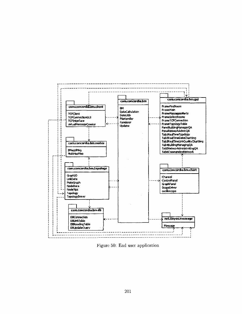
T
Figure 50: End user application
201
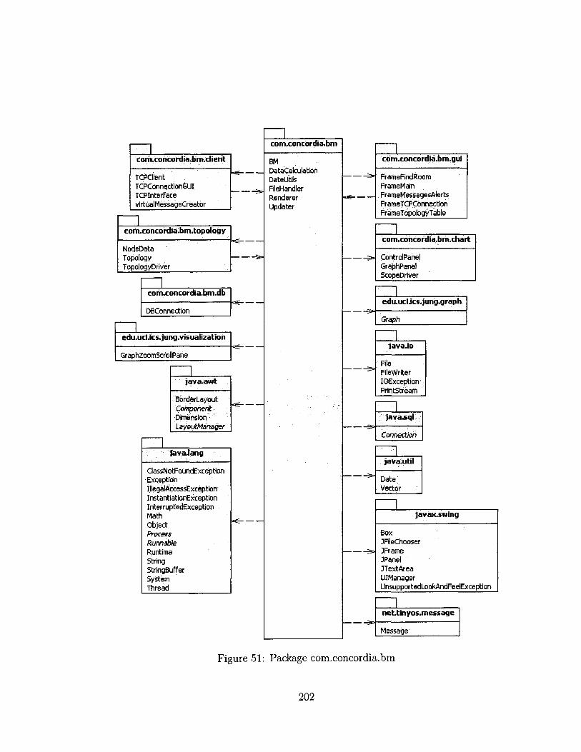
com.concordia.bm
com.concordia.bm.dient
TCPClient TCPConnectionGUr TCPInterface virtualMessageCreator
BM DataCalculation DateUtils FileHandler Renderer Updater
CDm.concordia.bm.gui
FrameFindRoom FrameMain FrameMessagesAlerts FrameTCPConnection FrameTopology Table
com.concordia.bm.chart
ControlPanel GraphPanel ScopeDriver
edu.uci.ics.jung.graph
Graph
java.io
Fife FileWriter IOException PrintStream
1 java.sql
Connection
java.util
Date Vector
]avax.swing
Box JFileChooser JFrame JPanel JTextArea UIManager UnsupportedLookflndFeelExceptlon
net.tinyos.message
Message
Figure 51: Package com.concordia.bm
202
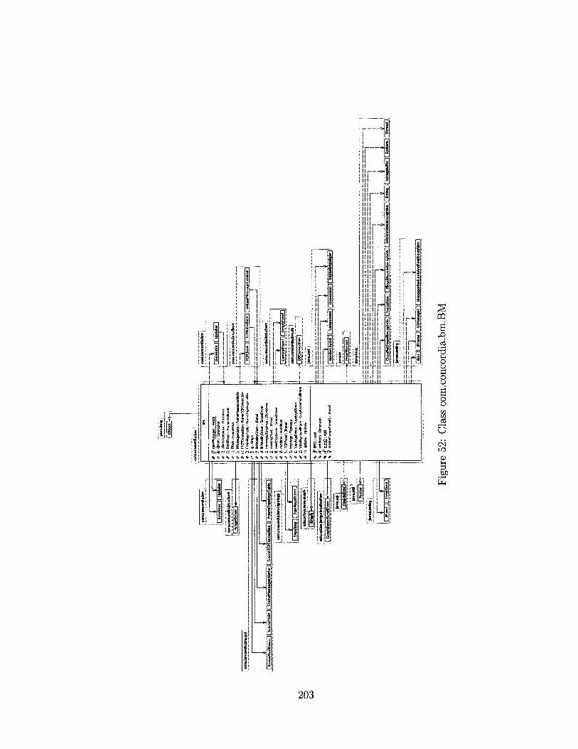
CQ s -O
T3 S-l O o a o o o o CO
o <M W QJ i—<
bO
203

java
.lan
g
Obj
ect
com
.con
cord
ia.b
m
Dat
aCal
cula
tion
i hu
mid
ity:
float
Q
lig
htlT
SR :
floa
t Si
lig
ht2P
AR :
floa
t S
pow
er:
float
£j
tem
pera
ture
; flo
at
§ tim
etof
ailu
re:
long
Q
tim
etof
ailu
reSc
ale
: lon
g
J® c
alcH
umid
ityQ
; fl
oat
# ca
lcLi
ghtlT
SRQ
: flo
at
cf
calc
Ligh
t2PA
R():
flo
at
J3
calc
Pow
erQ
: flo
at
d3 c
alcT
empe
ratu
reQ
: fl
oat
J3
calc
Tim
etoF
ailu
rep
: lon
g [J®
cal
cTim
etoF
ailu
reSc
aleQ
: lo
ng
# D
ataC
alcu
latio
n():
void
com
.con
cord
iaJb
m.t
opol
ogy
Nod
eDat
a
com
.con
cord
ia.b
m
Dat
eUti
ls
1
java
.lan
g
H
I M
ath
Str
ing
Figu
re 5
3: C
lass
com
.con
cord
ia.b
m.D
ataC
alcu
latio
n

java
.lan
g
Obj
ect
com
.con
cord
ia.b
m
Ren
der
er
com
xonc
ordi
a.bm
.top
olog
y
Nod
eDat
a
com
.con
cord
ia.b
m
Dat
eUti
ls
# J
5 PAT
E_FO
RMAT
_NO
W :
Stri
ng
4 J
1 DAT
E_TI
ME_
FORM
AT_N
OW
: S
tring
4
dP T
IME_
FORM
AT_N
OW
: S
tring
« =
<5>
dP D
ateU
tils(
): D
ateU
tils
^ dP
get
Cur
rent
Dat
einS
trin
gQ :
Stri
ng
^ J®
get
Cur
rent
Pate
Tim
einS
tring
Q :
Stri
ng
^ dp
get
Curr
entT
imei
nStri
ngQ
: S
tring
V
dP g
etPa
teFr
omSt
ringp
: P
ate
^ dp
get
Pate
Tim
eFro
mSt
ringP
: P
ate
^ dp
get
Pays
Diff
p : i
nt
* dP
getH
oursD
iffQ :
int
* dP
get
Mill
isec
PiffQ
: lo
ng
^ dP
get
Min
PiffQ
: lo
ng
^ J
3 get
Mon
thsP
iffQ
: in
t dp
get
SecD
iPfQ
: lo
ng
^ dP
get
Strin
gFro
mPa
teQ
: S
tring
%
dP
get
Strin
gFro
mD
ateT
itnep
: S
tring
^
dP g
etSt
ringF
rom
Tim
ep :
Stri
ng
^ dP
get
Tim
eFro
mSt
ringp
: P
ate
\ dP
get
Year
sDiff
p : i
nt
^ dP
mai
np :
voi
d
com
.con
cord
ia.b
m
T BM
D
ataC
alcu
lati
on
Figu
re 6
0: C
lass
com
.con
cord
ia.b
m.c
hart.
Cont
rolP
anel
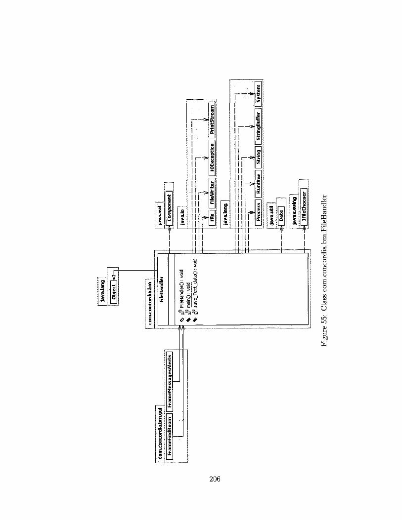
java
.lan
g
| O
bjec
t (<
3-i
com
.con
cord
ia.b
m.g
ui
Fram
eFin
dRoo
m
|| Fr
ameM
essa
gesA
lert
s
com
.conc
ordi
a.bm
File
Han
dler
Com
pone
nt
File
Han
dler
O :
voi
d ^
J8 m
ainQ
: v
oid
^ J®
sav
e_Te
xt_d
ata(
): vo
id
java
.aw
t
java
.io
i n ±
| Fi
le
|| Fi
leW
rite
r ||
IOE
xcep
tio
n]|
P
rint
Str
eam
java
.lan
g
i n ±
Proc
ess
\ |
Run
tim
e 11
Str
ing
11 S
trin
gBuf
fer
11
Sys
tem
java
.uti
l
Dat
e
java
x.sw
ing
H
JFile
Cho
oser
|
Figu
re 5
5: C
lass
com
.con
cord
ia.b
m.F
ileH
andl
er
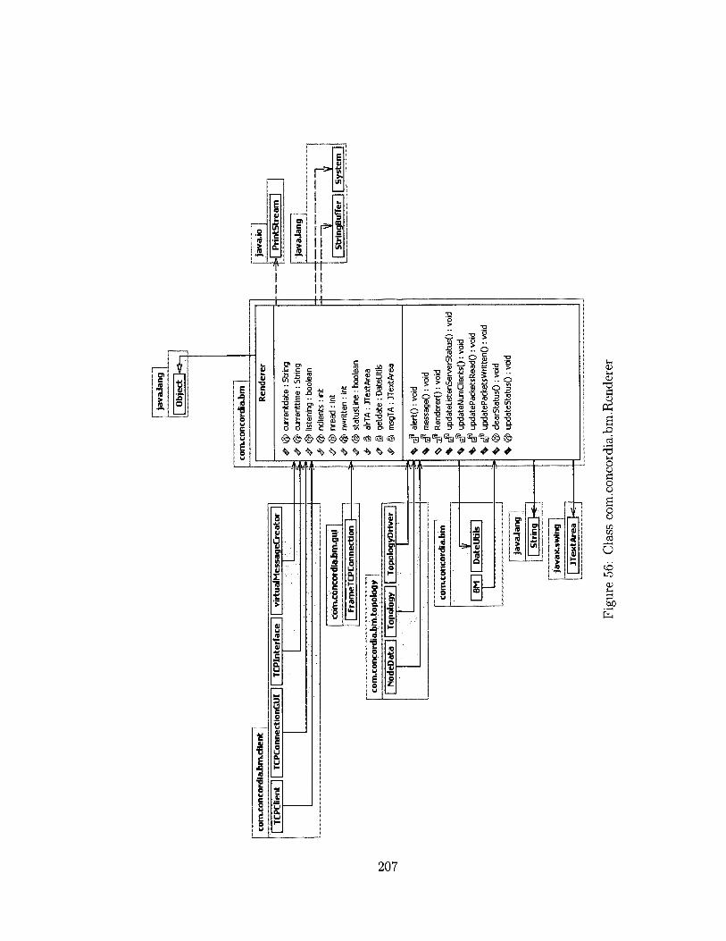
java
Jang
| O
bjec
t |«3—
com
.con
cord
ia.b
m.d
ient
TCPC
Iient
TC
PCon
nect
ionG
llI
|| TC
PIn
terf
ace
|| vi
rtua
lMes
sage
Cre
ator
to
o co
m.c
onco
rdia
.bm
.topo
logy
Nod
eDat
a ||
Topo
logy
||
Topo
logy
Pri
ver
com
.con
cord
ia.b
m
| B
M |
[D
ateU
tils
java
Jang
Str
ing
\*Sr
java
x.sw
ing
| JT
extA
rea
com
.con
cord
ia.b
m
Ren
dere
r
# #
curr
entd
ate
: Stri
ng
# #
curre
nttim
e : S
tring
#
<® li
sten
ing
: boo
lean
<®
ndi
ents
: in
t #
# nr
ead
: int
#
{§>
nwrit
ten
: int
#
# st
atus
Line
: bo
olea
n #
a al
rTA
: JTe
xtAr
ea
# §
getd
ate
: Dat
eUtil
s #
iS m
sgTA
: JT
extA
rea
%
t#
aler
t():
void
J3
mes
sage
():
void
(J
5 Ren
dere
rO :
void
^
J up
date
List
enS
erve
rSta
tus(
): vo
id
%
[J u
pdat
eNum
Clie
ntsO
: v
oid
\ o
f up
date
Pack
etsR
eadO
: v
oid
%
J3 upd
ateP
acke
tsW
ritte
nO :
voi
d \
# de
arS
tatu
s()
: voi
d %
#
upda
teS
tatu
sQ:
void
java
.io
-j»|
P
rint
Str
eam
java
Jang
i St
ring
Buf
fer
[| S
yste
m
Figu
re
60: C
lass
com
.conc
ordia
.bm.ch
art.C
ontro
lPan
el

Figu
re 8
7: C
lass
com
.conco
rdia.bm
.gui.Ta
b5Netw
orAdm
inistrati
ngQA

com.concordia.bfii
BM Updater
java.awt
BasicStroke Borderlayout Color . Component Container Dimension Font FontMetrks Graphics GraphicsZD GridBagConstraints GridBagLayout Gridlayout Image LayoutManager Point RerideringHirits Shape Stroke
java.io
File Fi leOutputSt ream FileWrlter IOException OutputStream PrintStream Print Writer Writer
java.lang
Class ' ClassNofcFoundException Double. Exception IllegdAccessException . InstantiationException Integer Math NoClassDefFoundError Object String StringBuffer System
com.concordia.bm.chart
Channel ControlPanel GraphPanel ScopeDriver oscilloscope
com.concDrdia.bfti.gui
FrameSelectRooms
edu.ud.ics.jung.graph
Graph
java.awt.event
ACHonEvent ActlonListener IteiriEvent Itemlistener MouseEvent MouseLOsterter MouseMotionListener Winder/Adapter WindowEvent . WMowUstener
javax.swing
JButton XhecNBox JFileChooser JFrame JPanel
J S c r o i P a n e JStider JTextField UIManager UnsupportedLookAreffeelException
javax.swing.event
ChangeEvent Changelistener
net.tinyos.message
Message
Figure 58: Package com.concordia.bm.chart
209

JavaJa
ng
I Obje
ct ha
-
com.
conc
ordiaJ
imxh
art j
Chann
el #
® co
brlndex
: int
#
plotCo
lors :
ColorQ
%
iff a
ddPoin
tO :
void
dP C
hannelO
: voi
d %
dp de
ar():
void
* rg<
findN
earestX
(): Poi
nt2D
% dp
saveO
ata():
void
* #
trimQ
: void
Basic
Strok
e
Poin
t2D
\
dP ac
tive :
boolean
<?
dP da
ta : V
ector
& dP
dataL
egend
: Stri
ng
& dP
graph
Panel
: Grap
hPanel
$
dP la
stPoin
t: int
& dP
mast
er: bo
olean
& dP
maxL
ength
: int
<S> dP
plotCo
lor :
Color
&
dP pl
otStrok
e : S
troke
com.co
ncordi
a.bm.
chart
I -j
Contr
olPane
l jav
awt
java.a
wt.ge
om
Zl_
%
IOEx
ception
|| W
riter
java-la
ng
•l
_JL
—1 J.
Class
II Cla
ssNotF
ound
Excep
tion 11
Exce
ption
|| M
ath ||
NoCla
ssDefF
oundE
rror ||
String
Buffe
r
Figu
re 8
7: C
lass
com
.conco
rdia.b
m.gu
i.Tab5
Netw
orAdm
inistrat
ingQA

com
-cqn
cord
iaJi
nri.c
hart
V G
raph
Pane
l j|
Scop
eDriv
er |
| os
cillo
scop
e
edu4
jciic
s.ju
ng.g
raph
Gra
ph I
java
Jang
Strin
g
java
.util
!
Has
htab
le
Vect
or
Java
&sw
ing
JBut
ton
II JC
heck
Box
II JS
Iider
jav&
awte
vent
j jav
ax.sw
ing
j jav
ax.sw
tag.ev
ent
{ | :
j
o-
, jav
ax.sw
ing
j jav
ax.sw
tag.ev
ent
{
j ite
miist
ewer
h^i
| }
JPan
el (o
—. I
Cfea
rage
Uste
Rer
}<h
It-- i
com
.con
cord
iaJi
m.d
iart
Con
trol
Pane
l
0 d"
legend
Active
: Ha
shtable
#
Ss legend
Edit:
Hashta
ble
# #
dear_d
ata :
JButto
n #
® co
nnect_
points
: JCh
eckBo
x #
® ed
itLegen
d : J
Button
•£>
loa
d_data
: JBu
tton
& ®
move
_down
: JB
utton
# @
mov
ejeft:
JButto
n 0
<® m
ove_rig
ht: JB
utton
move_
up :
JButto
n #
@ pa
nel: G
raphPan
el #
® re
set: J
Button
@
save_
data :
JButto
n &
<$>
scroll
ing: JC
heckB
ox
4> <
8? sh
owLeg
end :
JCheck
Box
&
timejo
cation
: JSI
ider
type :
String
+
® Y
AxisHe
x : JC
heckB
ox
# #
2oomJ
n_x :
JButto
n #
® zo
om_in_
y : J
Button
&
# zo
om_ou
t_x :
JButto
n ®
zoorn
_out_y
: JB
utton
# a
g : G
raph
i sele
ctedNlo
tes :
Vector
^
Si se
lectedR
eading
: Ve
ctor
% tip
action
Perform
edO :
void
^ J®
Contr
olPane
lO :
void
% d
P item
StateC
hanged
O :
void
% J
state
Chang
ed(): v
oid
% §
createL
egendE
ditO :
void
' Scop
eDrive
r: Scop
eDrive
r
.J
-f-
H
Fram
eSel
ectR
oom
s |
i PM
co
m.c
anco
rdia
.bm
com
.con
cord
ta.b
m.c
haff
~ b|
Cha
nnel
com
.con
cord
ia.b
m.g
ui !
java
.aw
t
"1
J_
Com
pone
nt |
[ G
ridB
agC
onst
rain
ts |
j G
ridBa
gLay
out
[ | G
ridLa
yout
[
Java
.aw
teve
nt
h—
T~
1 t
1 1
| A
ctio
nEve
nt I
Ite
mEv
ent
|
java
.io I
Prin
tStr
eam
1
java
Jang
|
ZL
"1.
"1
JL
Obj
ect]
j St
ringB
uffe
r ||
Syst
em
—
5H
JTeH
tFie
id"
java
x.sw
ing.
even
t
;H
Cha
ngeE
vent
Figu
re 6
0: C
lass
com
.con
cord
ia.b
m.c
hart
.Con
trol
Pane
l

': f l l l l l s t m m J l U f t l l ' i i <$ $ & $ $ £ # 0 • % v % v
! i ! l i l ! l | ; | ! i i l f l ! l l | ?» , ! , | i i l «
QJ fl 03 Oh JH Oh 03 S-l
o
^ o S 23
t? S-l O O C o o
o o 03
O r—1 <15 i-H
bfi
212

javaJan
g |
| Objec
t j<3—
| |
eonuon
corduJ
Kiuhar
t I
| Contr
dPanet
liGrap
hPand
|| Sco
peDriver
java
x.swing
JFrame
II JP
anel
to
I—i
oo
cam
xonc
ord
iaJj
mxh
a rt
i
&
<& c
onte
rtPa
ne :
JPa
ne!
<? 0
co
ntro
Pane
!: Co
ntro
tPan
el
cfrr
ver:
Scop
eDriv
er
# gr
oup J
d : i
nt
# #
mai
nfra
me:
JFr
ame
&
pane
l: G
raph
Pane
l
%
J5 cha
rtm
essa
gsO
: v
oid
^ riP
get
SoeQ
: D
imen
sion
* af
mai
nQ :
void
^
osa1
losc
ope<
); vo
id
li JL
i
] Bo
rderLay
out 1
r~Com
poffenT
l | Co
ntainer
| ["Dime
nsion
| j layo
ngaw
aggr
javM
intevet
Wm
dow
Adap
ter 1
1 W
induwL
vertt i |
Wmio
wtistow
y 1
favajo
7
~i
' 1
| IOExc
eptton
PrintStre
am [
javaJa
ngj
"T
EEEE
EE~E
EEEE
EEEE
EEEE
EEEE
EEEE
EEEE
EEEE
p—
EEEE
EEEE
EEEE
"——
1
| I
] I
_ "j?
^
^ ^
| ^
. |
I dass
NotFou
ndExce
ption {|
Exce
ption jfU
tegalAc
cessEx
ceptrotT
l| insta
nMation
Excep
tion [("
"inteoe
r | ["s
tring
ifstrtng
Buffer
H S
ystem"
! java
tcswlng
j
| JScr
oflPane
jHuiM
anaqer
"ll U
nsupporte
dLookA
ndFeelE
Kceptlo
n nfe
ttinyow
ttessage
H
M
essa
ge [
Figu
re 6
2: C
lass
com
.con
cord
ia.b
m.c
hart
.Osc
illos
cope

java
.lang
| O
bjec
t hg
—
com
.con
cord
ia.b
m
BM
1|
Upd
ater
com
.con
cord
ia.b
m.c
hart
Con
trol
Pane
l ||
osci
llosc
ope
com
.con
cord
ia.b
m.c
hart
Scop
eDri
ver
# i®
1 dat
eTim
eSta
rtDat
e : D
ate
# #
date
Tim
eSta
rtMilli
: lon
g #
msg
: M
essa
ge
# #
neig
hbor
s : V
ecto
r 4
%
NUM
_REf
lDIN
GS
: int
#
olds
elec
tedM
ote
: Vec
tor
# #
olds
elec
tedR
eadi
ng :
Vect
or
# #
pane
l: G
raph
Pane
l &
rend
erer
: Ren
dere
r 4>
<&
t: H
asht
able
&
<JJ>
tem
pmes
sage
: V
ecto
r #
# ty
pe :
Stri
ng
%
s# c
lear
_dat
a():
void
tf
fin
dCha
nnel
(): C
hann
el
%
J m
akeL
egen
dStri
ngO
: S
tring
^
iff m
essa
geR
ecei
ved(
): vo
id
\ iff
osc
opeR
ecei
ved(
): vo
id
^ J®
Sco
peD
river
(): S
cope
Driv
er
^ of
1 Sco
peD
river
O :
Scop
eDriv
er
%
tf
upda
teO
: vo
id
%
ffl
isM
oteI
DSe
lect
ed():
boo
lean
%
§
upda
teC
hann
els(
): vo
id
iff s
elec
tedM
otes
: Vec
tor
of s
elec
tedR
eadi
ngs:
Vec
tor
Figu
re 6
0: C
lass
com
.con
cord
ia.b
m.c
hart
.Con
trol
Pane
l

Figure 64: Package com.concordia.bm.client
215

com
.con
cord
ia.b
m.g
ui 1
1 Fr
ameT
CPC
onne
ctio
n
com
.con
cord
ia.b
m.d
ient
TCPC
onne
ctio
nGUI
TC
PInt
erfa
ce
to Oi
com
.con
cord
ia.b
m
Ren
dere
r
java
.io
Inpu
tStr
eam
11
Out
putS
trea
m
java
.lang
Thre
ad H
&-
java
.net
H
Inet
Addr
ess"
"] I
Soc
ket]
java
.lang
I
[ Th
read
fo
-i
com
.con
eord
ia.b
m.c
fient
TCPC
lient
Interfac
e : TC
PInterfa
ce
# ^
port:
int
^ ren
derer:
Rend
erer
Si die
ntSock
et: So
cket
# ipS
erver:
InetA
ddress
is
: Input
Stream
&
$ os
: Outp
utStrea
m
S pac
ketcou
nt: int
^
{3 th
: Threa
d %
con
nect():
boolea
n ^
rP dis
connec
tQ :
boolean
^
d9 mainQ
; void
%
SlP re
adPack
et(): b
yte[]
* #
runO :
void
V J
1 startd
ient():
void
^ gf
TCPC
lient():
void
* $
readN
(): by
te[]
__
__
__
__
__
__
, j
| i
. i
y ^
v ^
y j
Exce
ptio
n""!
I In
tege
Tl |
Nul
lPoi
nter
Exce
ptio
n ||
Obj
ect
|| R
tmna
We
j Tst
fing
[ |~
Strin
gBuf
fer
|
I
Figu
re 6
5: C
lass
com
.con
cord
ia.b
m.c
lient
.TC
PClie
nt

java
.aw
t.eve
nt 1
ja
vax.
swin
g j
| JP
anef
lo—
[
com
.con
cord
ia.b
m
Ren
dere
r k
-^
to
H-1 -a
com
.con
cord
iaJi
m.c
lient
£ TC
PCIie
nt 1
1 vi
rtua
lMes
sage
Cre
ator
Java
Jang
j
Strin
g H
H
Java
x^w
ing
v JB
utto
n 11
JLa
bell
| JP
anel
11
JTex
tFie
ld
com
.con
cord
ia.b
fruJ
ient
TCPC
onne
ctio
nGUI
# i®
dien
t: TCP
CIient
# IP
: String
#
i§> po
rt: Stri
ng
# ®
portln
t: int
# #
vmc :
virtual
Messa
geCreat
or #
S jLa
bel: JL
abel
# a
jLabelS
erverIP
: JLa
bel
4? l}
j jLa
belSer
verPo
rt: JLa
bel
# §
jPane
ll: JPa
nel
& S
J ren
derer:
Rend
erer
^ J®
action
Perform
edO :
void
<4. J
TCP
Connecf
cionGU
IO :
void
* S
geUPan
elQ : J
Panel
# J
TCPP
anel: J
Panel
# S
jButton
Conne
ct: JBu
tton
# '3
jButton
Discor
mect:
JButton
#
S Se
rverIP
: JTextF
ield
# 3
Serve
rPort:
JTextF
ield
javaw
t I
"1
1 i
.-
4 4
_,.
i t_
C
ompo
nent
II
Dim
ensi
on 1
1 G
ridB
aqC
onst
rain
ts |
| G
ridB
agta
yout
11
Lay
oufM
anag
er \
] ja
va£W
t.eve
nt
h =H
Act
ionE
vent
M
Obj
ect
Java
Jang
Figu
re 6
6: C
lass
com
.con
cord
ia.b
m.c
lient
.TC
PCon
nect
ionG
UI

java
.lang
| O
bjec
t
com
.con
cord
ia.b
m.d
ient
TCPC
lient
com
.con
cord
ia.b
m
Ren
dere
r K
-
com
.con
cord
ia.b
m.m
otes
H
BM
appl
Msg
"] I
Mul
tiHop
Msg
]
net.t
inyo
s.m
essa
ge
Mes
sage
H
s-
com
.con
cord
ia.b
m.c
lient
TCPI
nter
face
# bm
appl
msg
: BM
applM
sg
# <§
> m
sg :
Mes
sage
#
<9>
mul
tihop
msg
: M
ultiH
opM
sg
# pa
cket
: by
te[]
# pa
rent
: b
yte[
] 0
# re
nder
er: R
ende
rer
3 pa
cket
amty
pe :
int
# Q
pac
ketb
aseo
ffset
: in
t #
S pa
cket
data
leng
th :
int
# Q
par
enta
mty
pe :
int
# S
pare
ntba
seof
fset
: int
#
3 pa
rent
data
leng
th :
int
%
iJ3 m
ymes
sage
Rec
eive
dO :
voi
d J>
TC
PInt
erfa
ceQ
: v
oid
H
BM
com
.con
cord
ia.b
m
java
.lang
~3L
java
.util
Vect
or
i Ex
cept
ion
|| St
ring
Figu
re 8
7: C
lass
com
.conc
ordi
a.bm
.gui.T
ab5N
etwor
Adm
inist
ratin
gQA

com
.con
cord
ia.b
m.c
lient
TCPC
onne
ctio
nGUI
com
.con
cord
ia.b
m.g
ui
Fram
eTC
PCon
nect
ion
to
I—' co
com
.con
cord
ia.b
m
Ren
dere
r H
S-
com
.con
cord
ia.b
m.m
otes
BM
appl
Msg
[|
Mul
tiHop
Msg
| ja
vaJa
ng
17-
-t1
|| Th
read
h
a-i
com
.con
cord
ia.b
m.c
lient
virt
ualM
essa
geC
reat
or
# <3
> bm
applm
sg :
BMap
plMsg
#
@ m
sg :
Mes
sage
4>
m
ultiho
pmsg
: M
ultiH
opM
sg
4> ®
pa
cket
: byt
e[]
s® p
acke
tcou
nt: i
nt
& <%
> pa
rent
: by
te[]
# re
nder
er: R
ende
rer
4 se
qno
: int
#
@ t
h i T
hrea
d &
S pa
cket
amty
pe :
int
4> (
2 pa
cket
base
offs
et: i
nt
3 pa
cket
data
leng
th :
int
$ 3
pare
ntam
type
: in
t S
pare
ntba
seoF
fset
: int
©
par
entd
atal
engt
h : i
nt
^ J®
mym
essa
geR
ecei
ved(
): vo
id
% •
§ ru
n():
void
^
star
tvirt
ualm
achi
neO
: vo
id
% J
® s
topv
irtua
lmac
hine
O :
void
^
g!P
virtu
alM
essa
geC
reat
orO
: voi
d
H
BM
=H
Prin
tStr
eam
com
.con
cord
ia.b
m
java
.io
java
Jang
T En
cept
ion
|| M
ath
|| O
bjec
t | [
Rtin
nflb
te l
1 S
trin
g ||
Strin
gBuf
fer
|| Sy
stem
H
Vect
or
java
.util
Figu
re 6
8: C
lass
com
.con
cord
ia.b
m.c
lient
.Vir
tual
Mes
sage
Cre
ator

Figure 69: Package com.concordia.bm.db
220

java
.lan
g
Obj
ect
f<3—
java
.sql
| Cw
wertr
on
com
.con
cord
ia.b
m.d
b
DB
Con
nect
ion
dbco
n: C
onne
ctio
n «=
L|
BM
|
J3 D
BCon
nect
ionQ
: v
oid
V J5 g
etC
onne
ctio
nQ :
Con
nect
ion
^ [J
5 mai
nQ :
voi
d
3»|
Pri
ntS
trea
m
com
.con
cord
ia.b
m
com
.con
cord
ia.b
m.d
b
1 "1
JL
I D
BLi
nkTa
ble
|| D
BR
eadi
ngTa
ble
|| D
BU
pdat
eQue
ry
java
jo
java
.lan
g
'JL
1 "1
"i
Cla
ss I
I C
lass
Not
Foun
dEK
cept
ion
|| S
trin
g ||
Str
ingB
uffe
r ||
Sys
tem
java
.sql
'It
1 |
Dri
verM
anag
er
| S
QLE
xcep
tion
|
iH
Vec
tor
java
.uti
l
Figu
re 6
0: C
lass
com
.con
cord
ia.b
m.c
hart
.Con
trol
Pane
l

Figu
re 8
7: C
lass
com
.con
cord
ia.b
m.g
ui.T
ab5N
etw
orA
dmin
istr
atin
gQA

java
Jang
Obj
ect
com
.con
cord
ia.b
m.d
b
DB
Rea
ding
Tabl
e
# fy
co
untre
adin
gTab
leVa
lues
: in
t #
# re
adin
gTab
leVa
lues
: V
ecto
r #
# th
: T
hrea
d #
(2 c
on :
Con
nect
ion
^ J0 D
BRea
ding
Tab!
e():
DBR
eadi
ngTa
ble
%
J® r
un()
: vo
id
%
J3 Upd
ateR
eadi
ngsT
able
Valu
esQ
: v
oid
com
.con
cord
ia.b
m.d
b
DB
Con
nect
ion
com
.con
cord
ia.b
m.to
polo
gy
Nod
eDat
a
Figu
re 8
7: C
lass
com
.conc
ordia.b
m.gu
i.Tab
5Netw
orAdm
inistr
ating
QA

javaJang
| Object |o—
com.concordia.bm.db
DBUpdateQuery
# <9 countLinksTableValues : int 0 # countreadingTableValues : int # <S> LinksTableValues : Vector + readingTableValues : Vector # & con : Connection
« ; 1 DBConnection
* dP chartlinkqualityQ : Vector ^ dP chartreadingsQ : Vector <> dP DBUpdateQueryO ; DBUpdateQuery ^ dP DBUpdateQueryO : DBUpdateQuery * dP finddatetimesQ ; Vector % dP findroomsQ : Vector ^ dP getdatetimeLastMsgRecp ; Date
dP getdatetimeSeenbyApplQ : Date ^ dP getdatetime5tarting() ; Date ^ dP getDistributionofParentsChildrenoverTimeQ : Vector ^ dP getDistributionOverTiimeQ : Vector % dP getLampsONOFFQ : Vector % dP getlocxp : double * dp getlocyp : double % dP getLostCountQ : long ^ dP getMessagesCountQ : long % dP getMinMaxAverageQ : Vector
dP getMotesListQ : Vector % dp getMotesRooroQ : String * dP getParentsChildrenlistp : Vector % dP getparentslistO : Vector
dP getPercentageOverTimeO: float \ dP getpowerStartO : float ^ dP getPowerTimetoFailureUsage(): Vector ^ dP getroomQ : String ^ dp insertMoteinMotesTO : boolean % dP isMoteIDinMotesT(): boolean % dP updatedatetimeLastMsgRecO : boolean ^ dP updatedatetimeSeenbyAppl(): boolean % dP updatedatetirneStartingQ : boolean ^ dP UpdateLinksTable(): boolean ^ dP UpdateLlnksTableValues(): boolean ^ dP UpdatelocxO : boolean ^ dp UpdatelocyO : boolean % dP UpdateMotesTableO : boolean % dP UpdatepowerStartO : boolean ^ [J3 UpdateReadingsTable(): boolean ^ dp UpdateReadingsTableValues(): boolean % dP UpdateroomO : boolean
com.concordia.bm.db
com.concordia.bm.topology
H NodeData
Figure 73: Class com.concordia.bm.db.DBUpdateQuery
224

com.concordia.bm.chart
ControlPanel
com.concordia.bm.topology
NodeData Topology
edu.uci.ics. jung.gr aph
Graph Vertex
java.awt
BordeiiayOut Color Component Container Dimension Font . GridBagConstraints GridBagLayout GridLayout LayoutManager Rectangle
java.util
ejection HashSet iterator Set
, javax.swing
AbstradButton BorderFactory BoxLayout ButtonGroup Icon JButton JCheckBox JComboBox JFrame: JLabel JPanel JRadioButton JScrollPane JTabbedPane JTextArea JTextField UIManager UnsupportedLookAndFeelException
com.concordia.bm.gui
FrameFindRoom FrameMain FrameMessagesAlerts FrameSelectRooms FrameTCPConnection FrameTopologyTable PanelBuildingManagerQA PanelNetworkAdminQA TablRealTlroeTopology Tab2RealTimeDataChartting Tab3RealTirneLinkQualityChartting Tab4BuildingManagingQA TabSNetworAdministratingQA Tab6CommandingNetwork zzzTextfields
com concordia.bm
BM FileHandler Renderer
com.concordia.bm.dient
TCPClient virtualMessageCreator
java.awt.event
ActionEvent AttiortistenSr
java.lang
CiassNotFoundException Float IllegalAccessException InstantiatlonExceptlon Object String StringBuffer
javax-swing.border
Border TitledBorder
Figure 74: Package com.concordia.bm.gui
225

o & fl
• •—I fa QJ a o3
£
'3 bO - O
oj '-3
(-1 O o d o o o o 73 m o3
o lO t-a> fcuO
226

com.concordia.bm
BM
com.concordia.bm.gui
FrameTCPConnection
javax.swing
JFrame |<3—
•5*
com.concordia.bm.gui
FrameMain
# S
jpanel3 : JPanel jpanelMoteDetailandRest: JPanel jpanelTopologyandRunTime : JPanel boxMoteDetail: Box boxRunTime : Box fFindRoom : JFrame fMsgAlrts : JFrame fTCPconn : JFrame jMenuItemFindRoom : JMenuItem jPanelBuildingManagerQA : PanelBuildingManagerQA jPanelNetworkAdminQA : PanelNetworkAdminQA linkqualityChart : JPanel readingChart: JPanel serialVersionUID; long topologyScrollPane : GraphZoomScrollPane
\ # EnableFrames(): void <> FrameMainQ : FrameMain % Q getJMenuItemControls(): JMenuItem % Q initialize(): void
# jContentPane: JPanel jFileMenu; JMenu jMenuItemMessagesAlerts : JMenuItem jMenuItemOpen : JMenuItem jMenuItemProperties : JMenuItem jMenuItemQuit : JMenuItem jMenuItemSave: JMenuItem jMenuItemServerConnection : JMenuItem jOptionsMenu : JMenu mainMenuBar: JMenuBar
Figure 76: Class com.concordia.bm.gui.FrameMain
227

J t l

javax.swing
| 3Frame~l<a~
com.concordia.bm.gui j
FrameSelectRooms
<§> g : Graph 4> <S> group : ButtonGroup
i® ScopeDriver: ScopeDriver & 0 selectedMotes : Vector
<8> selectedReading ; Vector # 0 temp : Vector # © jLabel: JLabel # !2 jLabel 1 : JLabel # 51 jLabel2 : JLabel # S jLabel3 : JLabel
© jLabeH : JLabel # S jLabelS : JLabel
© jLabel6Humidity : JLabel & © jLabel6Light: Xabel <#> iS jLabel6Power; JLabel # © jLabeltemperature : JLabel # S serialVersionUID : long # © type : String
% dP actionPerformed(): void dp FrameSelectRooms(): FrameSelectRooms
<I> dP FrameSelectRooms(): FrameSelectRooms > dP getMotesListChartQ : void % dP mainQ : void * a nitializeO : void
© ButtonCANCEL : JButton a ButtonOKl : JButton
# © CheckBoxALLMotes : JCheckBox a ComboBoxMotel : JComboBox
# a ComboBoxMote2 : JComboBox a ComboBoxMote3 : JComboBox a ComboBoxMote4 : JComboBox
& © ComboBoxMote5 : JComboBox & a ContentPane : JPanel # © Panel: JPanel # a Panel 1 Buttons : JPanel
© PanelReadings : JPanel a RadioButtonhumldity : JRadioButton
& © RadioButtonLight: JRadioButton a RadioButtonpower; JRadioButton © RadioButtontemperature : JRadioButton
# © motesList: Vector
com.concordia.bm.chart
- - j ControlPanel |
Figure 78: Class com.concordia.bm.gui.FrameSelectRooms
229

javaw
tevent
j {av
axvin
g 1
t-tm
iitm
mm
^y^
\ JFra
me [<3
—i
to
CO
o
com.con
cordia.
bm.gu
i |
FrameTC
PConn
ection
' 0
clie
nt:
TCPC
Sent
'
IP :
Strin
g '
port
: St
ring
' %
po
rtln
t: in
t *
vmc:
vir
tual
Mes
sage
Cre
ator
>
Si
fMai
n : F
ram
eMai
n >
3 jt
abel
: JL
abel
'
jLab
elSe
rver
lP :
JLa
bel
' ilj
JLa
belS
erve
rPor
t: JL
abel
'
jPan
ell:
JPan
el
' &
re
nder
er:
Ren
dere
r *
(S s
eria
lVer
sion
UID
: lo
ng
> -
Si T
CPP
anel
: JP
anel
&
&
jBut
tonC
onne
ct:
JBut
ton
&
JBut
tonD
isco
nnec
t: JB
utto
n 4'
3
jCon
tent
Pane
: P
anel
Se
rver
IP :
JTe
xtFi
eld
&
tS
Serv
erPo
rt:
JTex
tFie
ld
%
t£p
actio
nPer
form
edO
: v
oid
^ $
Fram
eTC
PCor
mec
tionO
: vo
id
%
getfM
atr<
) : v
oid
* &
ge
tJPa
neK
): J
Pane
l *
Q
initi
a(iz
e():
void
favaw
t !
'JL
Comp
onen
t j
javaw
tevent
I
"i i
Contai
ner ||
Dime
nsion
I !
I fr
•
-f •
GridB
agCons
traints"1
j GridB
agLayo
ut 4ay
putW
£aagfir
.if Re
ctangle
|
Action
Event
| I j
avaJan
g j
sH O
bject |
Figu
re 7
9: C
lass
com
.con
cord
ia.b
m.g
ui.F
ram
eTC
PCon
nect
ion

com.concordia.bm
BM com.concordia.bm.topology
Topology
javax.swing
JFrame ]o—
com.concordia.bm.gui |
FrameTopology Table
# <&> g i Graph # <3> topologyTableDataModel: DefaultTableModel # S alterparentl : int $ S alterparentl LQ : int
iS alterparent2 : int & SI alterparent2LQ : int # S color i Color # i3 datetimeActiveStart: String
SI datetimeCurrent: String # a humidity : int # S IsBase : boolean & S isLampON : boolean & ® jTable : JTable 4 © light 1 : int # Iight2 : int # S locx : int # S locy : int # ® motelD : int
Q parent: int S parentLQ i int © powerCurrent: int
# (B powerStart: int # S powerStartDate : String # © room : String # 3 seqNo : int # ® serialversionuiD : long 4> S temperature : int & (3 timeToFailure : long ^ S topologyTableColumns : Object[] # S topologyTableData : Object[][]
% actionPerformedO : void ij® FrameTopologyTablef) : FrameTopologyTable
% J 8 main(): void * t f setGraph(); void ^ J® sortColumn(): void % SI initializeO void % (2 setTableQ : void
a jButtonClose : JButton # ffl jButtonPrint: JButton •4* (3 jButtonRefresh ; JButton & SI jButtonSave : JButton # 3 jContentPane : JPanel # © jPanelButtons : JPanel & SI jScrollPaneTablel : JScrollPane
Figure 80: Class com.concordia.bm.gui.FrameTopology Table
231

tava>Lswing j
I JPanel |<3~
coauancordiaJmguTj PanelBuild tngManagerQ A
/ <3> tabteDataModsl: DefauItTahleModel 3 dateTimefront: Date Q DateTlmeLongFrom: long Q DateTlrrteLcngTo: long
& fi datetimeto : Date & Sh JLabel: JLabel & Q JLabelt: JLabel # £ jLabellO : JLabel & (2 fl.abe!13 : JLabel
© ILabelH i JLabel ^ © JLabellS : JLabel & Q (Labell52: JLabel
3 JLabell6 : a.ebel ^ S JLabel laistDateTlmetot: JLabel ^ fL abel 16ListRocmsTo : iebel & © ilabeC : JLabel
(3 jLabet29 : JLabel & £ jLabeM : JLabel # S J.abe!6 : Jlabel & 3 fl.abel9: JLabel & © (LabelDatatype : JLabel & © (Table : JTable
© selectecWotes : Vector # S serialVersionUID: long # fl taWeCohjmns : Ob(ect[] + Q tableData : Ob|ect[]0 & a topology TableDataMode! 1 : DefaufcTaWeModel
* actionPerformedO ; w*1
^ -J5 getOateTtmeFromO: void ^ getOateTimeToO: vcwJ V # MessageO ; void ^ tIP PanelBuildngManagerQAQ : PanelBuildingManagerQA V get Topology TableOataModetO : Oefau&TabteModel ^ Q mftiateeO : void
& 3 (ButtonChartSelectftoom : JButton <P Si jButtonListSelectRoom Button & S (ButtonPrint; J3utton & fi (ButtonReset: JButton
Q IButtonSave : JButton a (BuKcnShow: JButton
& S iButtonTabteSelectRooms : JButton ^ fl fCheckBoxChart Average : JCheckBox & (2 (CombcBoxChsrtAverageof; jComboBox & © JComboBoxCbartDatatype: JComboBox
© (ComboBoxGiartlnterval i JComboBox (S (ComboSoxDIstributicnTempHumEtc: XomboBctt 3 }Combo8oxLlstDateTime: JComboBox ffl (ComboBoxLlstRoomsAvg: JComboBox
& uS )Combo8oxPercentageTemjiKum£tc: XomboBox & & JComboBoxTabteMinMaxAvg : JComboBox
la Pane1: JPanel fl iPandl: JPanel 0 panel 10 : JPanel
# tl) panellOl: Panel 4" A JPanefc: JPanel & <2 jpanel3: Panel & © jPaneH : JPanel & Q (Panels : JPanel # Q (Panels i JPanel
S panef7 : JPanel & S panels i JPanel & © PaneButtoru : JPanel
<2 jRadtoBuKcnChart: JRaSeSutton & Q padoButtonDistributlonTempHurnEtc : JRadioButton ^ 0 fcadioButtonLampstatusOistraiutran : JRadioButton 4> a WadioButtonList: JRadioRjtton v* S ladioButtonLlstOateTime : JRadioButton $ Q (R acSoButtonListftooms : JRadioButton
G P-adjoButtoriPercentageTempHumEtc: JRacfioButton '3 jRacfeo&JttcmTaWe : JRadioButton
& a (RadioButtonTaUeMinMaxAvg : JRadioButton 4> S iScrcllPaneTabtel; JSCTOCP«»
3 jtextfielc&^e Prom : JTextField # fii JtextfieldDateTo : JTextFidd
© (TextFleldLlstDateTbneFroml: JTextFfetd 3 (TextFieldUstDateTlmeTol : JTextField
<? @ (TextFieldListRoomsFrom: JTextField •P & {TextF EdListRoomsTo : JTextField & S fTextFtekfTaUaPercentageFrom : JTextField
<3 (Textfi^dTMePercentagelo: JTextField ^ © Messages: JTextField
Figure 81: Class com.concordia.bm.gui.PanelBuildingManagerQ
232

| j avax .swing
| JPanel l o —
com.concordia.bm.guij
PanelNetworkAdminQA
# <§> tableDataModel: DefaultTableModel # dateTimefrom : Date
S DateTimeLongFrom : long S DateTimeLongTo : long
& S datetimeto : Date # Si jlabell02 : JLabel
Q jLabelllO : JLabel <S> Q jLabel26: JLabel # S jLabel291: JLabel
a jLabel3 : JLabel # 3 jLabel42 : JLabel # Si jLabel62 : JLabel <(> 3 jLabel92; JLabel
3 jLabelDatatype2 : JLabel # 3 jTable : JTable ^ (it selectedMotes : Vector # 3 serialVersionUID ; long # S tableColumns : Object[] # a tableData : ObjectDD
^ J 3 actionPerformedO : void ^ J® getDateTimeFromO : void ^ J® getDateTimeToO : void ^ Messagef): void ^ J 8 PanelNetworkAdminQAO : PanelNetworkAdminQA ^ a initialize;): void
# S jButtonChartSelectRoom2 : JButton # S jButtonPrint: JButton # a jButtonReset2 : JButton ^ Sj jButtonSave : JButton # 3 jButtonShow2 : JButton & © j8uttonTable5electRooms2 : JButton # a jCheckBoxChartAverage2 : JCheckBox & Sj jComboBoxChartAverageof2 : JComboBox & a )ComboBoxChartDatatype2 : JComboBox 4" a jComboBoxChartlnterval2 : JComboBox # S jPanel: JPanel & S jPanell 1 : JPanel 4> ® jPanel22 : JPanel 4 S )Panel32 : JPanel <f a jPanel42 : JPanel 4> S ]Panel52 : JPanel i> S |Panel72 : JPanel
S jPanelButtons : JPanel & S jRadioButtonChart2 i JRadioButton & a jRadioButtonPowerUsageAvg : JRadioButton
S jRadioButtonTable2 : JRadioButton a jRadioButtonTableDistributionChild : JRadioButton S jRadioButtontablelistofParent: JRadioButton
# a jRadioButtonTablePowerUsageTimetoFailure : JRadioButton & a jRadioButtonTableShowMessagesLost: JRadioButton + § JScrollPaneTablel : JScrollPane & S jtextfieldDateFrom2 : JTextField v* a jtexttieldDateTo2 : JTextField v* a Messages2 : JTextField
Figure 82: Class com.concordia.bm.gui.PanelNetworkAdminQA
233
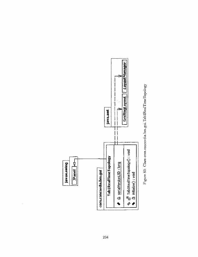
Figu
re 8
7: C
lass
com
.con
cord
ia.b
m.g
ui.T
ab5N
etw
orA
dmin
istra
tingQ
A

java
x.sw
ing
(O
co
oi
java
x.sw
ing
JPan
el
JPan
el
<3—
com
.con
cord
ia.b
m.g
ui
Tab2
Rea
lTim
eDat
aCha
rtti
ng
# (3
re
adin
gCha
rt:
JPan
el
# Q
se
rialV
ersi
onU
ID :
long
<S>
J3
Tab2
Rea
lTir
neD
ataC
hart
ting(
): v
oid
%
0 in
itial
izeQ
: vo
id
java
.aw
t
"1
'1 JL
C
ompo
nent
G
ridB
agLa
yout
n
Figu
re 8
4: C
lass
co
m.c
onco
rdia
.bm
.gui
.Tab
2Rea
lTim
eDat
aCha
rttin
g

java
K.s
win
g
to co
Ol
JPan
el
java
x.sw
ing
JPan
el
JPan
el
com
.con
cord
ia.b
m.g
ui
Tab3
Rea
lTim
eLin
kQua
lityC
hart
ting
# ®
lin
kqua
lityC
hart
: JP
anel
#
Q
seria
lVer
sion
UID
: lo
ng
<> J
8 Ta
b3R
ealT
imeL
inkQ
ualit
yCha
rttin
g():
void
%
0
initi
aliz
e():
void
java
.aw
t
"1
Com
pone
nt:
Grid
Bag
Layo
ut
Layo
utM
anag
er
H
JL
Figu
re 8
5: C
lass
co
m.c
onco
rdia
.bm
.gui
.Tab
3Rea
lTim
eLin
kQua
lityC
hart
ting
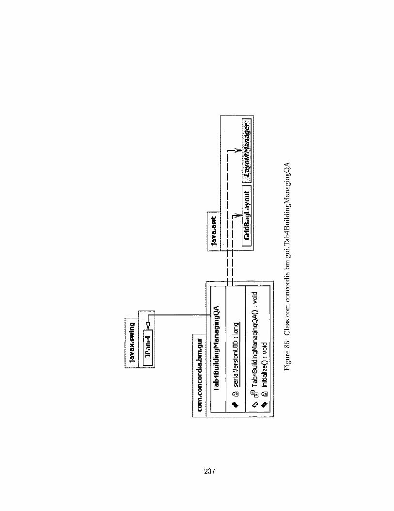
Figu
re 8
7: C
lass
co
m.c
onco
rdia
.bm
.gui
.Tab
5Net
wor
Adm
inis
tratin
gQA

java
.aw
t 1 i
Gri
dBag
Layo
ut
Layo
utM
anag
er
Figu
re 8
7: C
lass
co
m.c
onco
rdia
.bm
.gui
.Tab
5Net
wor
Adm
inis
trat
ingQ
A

Figu
re 8
7: C
lass
com
.conc
ordi
a.bm
.gui
.Tab
5Net
wor
Adm
inist
ratin
gQA

Figu
re 8
9: P
acka
ge c
om.c
onco
rdia
.bm
.mot
es


LtakedMetsage 1 . ! lsubriws«-2> r H )
t«rwencor<ttaJ>m.cllent ! j TCPlnterface 1 rVjrtuatltessaoeCreatoT"
conrMontonKaJimjRotetj
# OEPMAT J ESSAGE IZE i In
% etemert56e_dataQ : Irt * >Jt> riemantawgts.dataQ ; nt \ J? get_dataO: shortQ % getjdO: short * J1 get.onsjrwcttO: ht V J* get_arighss£poO : short % # 9et_seqno(>: short * # grt.souwaddrO:« % £ getJ*K): Short % & getElement_dat«0: short % £ ge«WngjiataO s Strtig * d¥ ttArray_detaQ: bootear V 4P HAfWjdO ; boolean ^ gjP frArT9yTorioir>addrO; boolean % J1 ttArrayjyigireeqnoO; boolean \ $ iiAfray_»eqno()= boolean % -M isArrayjsotfcead^Q: boolean % 5? teArrayjUQ : boolean % J* teSqwd-dataQ : boolean % # frSqnedJdO ; boolean % J1 HStQned_origiradclr<): boolean % jjp ttSyied_ongn»e<ino(): boolean % P isSgned_seqne<): boolean % iif isSigned.wureesddrO: boolean % jp BSignedJtIO: bodean <> RJUHopMigO : void ^ i2 MiAMocMsgO: void
£ MJtWopMsg()! void ^ -J1 MtiSMopMsgO: void <;> MiiUHooMsg(); void ^ $ MJtHopHsg(): void ^ $ MJUMopMsgO : void ^ / MiitlHopMsg(): void % rwmOimensionsjte«0: int % J1 numEtemertsjdataO: « % numQefnent s_data(): W % offset.detaO: rt % 5p offset.!*) :** % rffset.orlginaddrt); W % .J" offset.orlQlnsewO ' int % g offset_seqnoO : W % # offs«.sourceaddr(>: int * ,J> ofFset_t«0t I* % # cffsetBis.dataO: int % J1 offseffibjcK): int % of fsetBts.originaddrt): Int % if off»etM$_ori«n«qnoO • W % 5? offsetB»«_seqnoO : « * offsetSts ourceaddrO: int % j6 offieteitsjtdO: Int % Sp setjiataQ: void \ dP«tJdOJ»oid V # set_orttfneddr() • void % ;tP set_ortginseqnoO i void * J3 set_seqno(); void % $ set.sourceaddrO: void % J3 »<JttfO; void * J1 set0emert_data() : vold % J1 setStrhg.dalsO: voU \ -f sSeJK): int * $ soejjrighsdtfrO • W % 'Jt1 sne.origirwflnoO : W % slze.seqnoO : ^ % si?e jJOurcsadtK): int % J'sBejUO:** % $ siKBts_id(): int % # siteBks.orifnaddrO : mt ^ $ seeBts.ori nsegnoO: int ^ £ soeBis eamO : Int \ siwB»s_Murc«ad±0: int % yf sftaBts Jtl() i Int % toStrngO ; String % totaBbe_dafa() : M » df1 tcta!5i;e&ts.data(): H
convcon«irdtai»m.topo>ogy j [ NotteOata"ll TopotowPrtver 1
—1 i J_
! | flrraylndewOutOfBounJsEwceptlon jl IBepalArqiMwentEwcepttoir]I long ll Hatti irartng II arlnqBuffer |;
: neUfoyos. message < — — HenaaeH
Figure 91: Class com.concordia.bm.motes.MultiHopMsg
242

Vat*.
—
•
S S L
Figure 92: Package com.concordia.bm.topology
243

java
Jang j
I O
bjec
t ha
-.
i co
m^o
ncar
*fia
.bm
.topo
logy
Gra
phlO
^ badG
raphQ bo
olean
* rese
tPrefsQ
: boole
an
^ ©
saveGra
phQ : b
oolean
%
0 wr
iteJPEQro
ageQ : b
oolean
conv
conc
ordi
alm
itopo
logy
I N
odeD
atal
l To
polo
gy |
1 edi
Mic
Mcs
.jung
.gra
ph >
edu.
ucljc
s4un
g.vi
5iia
1tza
tii]ii
I
offe
redl
mag
e H
Rtin
derc
dhnz
g?
J_
I I B
uffe
tedR
eade
r M
file
||
Hte
flotF
ound
Exce
ptio
n [|
Rle
Out
putS
tream
11
Rle
Rea
der
[} I
OEx
cept
ion
| j Q
utpu
t&re
am If
Ptin
tWri
ttg[|
Rea
der
\
java
.lang
3L
I I |
Dou
ble
ll Ex
cept
ion
}j In
tege
r ||
Pro
cess
| ["
"Run
time
)f S
tring
jSt
ring
Buf
fer"
Java
uutfl
r-i—
* I
j n
•?
i ?
. |
Has
hSet
Jmaq
eZO
|
i |av
ax.sw
tng
M
JFile
Choo
ser
|
Figu
re 2
62: C
lass
com
.conc
ordia
.bm.to
polog
y.Top
ology
Drive
r
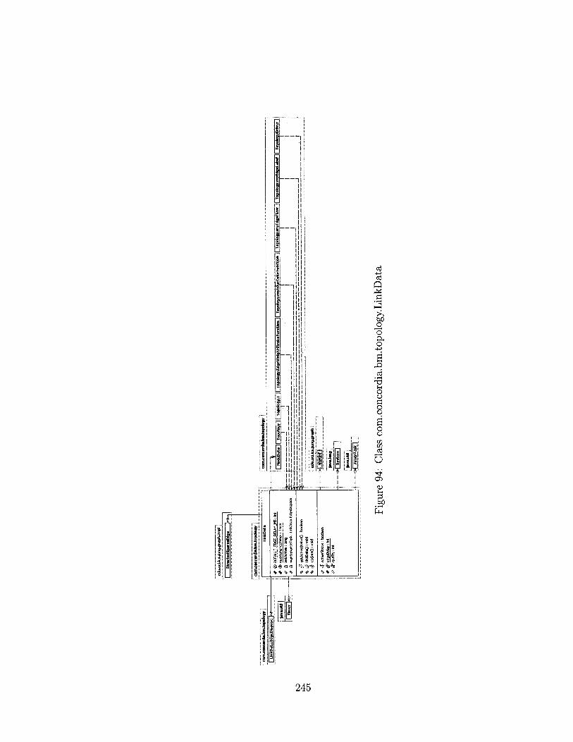
245

Figu
re 8
7: C
lass
com
.conc
ordi
a.bm
.gui
.Tab
5Netw
orA
dmin
istra
tingQ
A

03 03 Q
<x> -a o bO
O
o a o s d >-. o o c o o o o CO
CO
03
5 CD
a> P tuO
CVI

edu.
uci.i
cs.ju
ng. v
isua
lizat
ion
Wsu
aliz
atim
VKne
r.TaQ
tTip
Ust
erie
t' }O
j |
Obj
ect
ha—
java
.lan
g
I
edu.
uci.i
cs.ju
ng. v
isua
lizat
ion
Vis
ualiz
atio
nVie
wer
K
-
com
.con
cord
ia.b
m.t
opol
ogy
Nod
eTip
s
^ <§
> w
: V
isua
lizat
ionV
iew
er
%
$ ge
tToo
lTip
Text
():
Stri
ng
J N
odeT
ipsQ
: v
oid
1 H
P
icfe
Sup
p5fi~
l
com
.con
cord
ia.b
m.t
opol
ogy
- -|
Topo
logy
|
edu.
uci.i
cs.ju
ng.g
raph
•t~-1
:
i IS
Bap
sli^
^;!
edu.
uci.i
cs.ju
ng. v
isua
lizat
ion
H
Poi
nt
java
.aw
t
java
.aw
t.ev
ent
Mou
seE
vent
java
.aw
t.ged
m
M
P°in
*2D
java
.lan
g
„ 1
Exc
epti
on
[| S
trin
g
Figu
re 2
66: C
lass
com
.conc
ordia
.bm.to
polog
y.Top
ology
Drive
r

>5 bO O 'o a, £
o a o
S-l o o c o o
o o
a3 o CO os a> S-H
bJ3
249
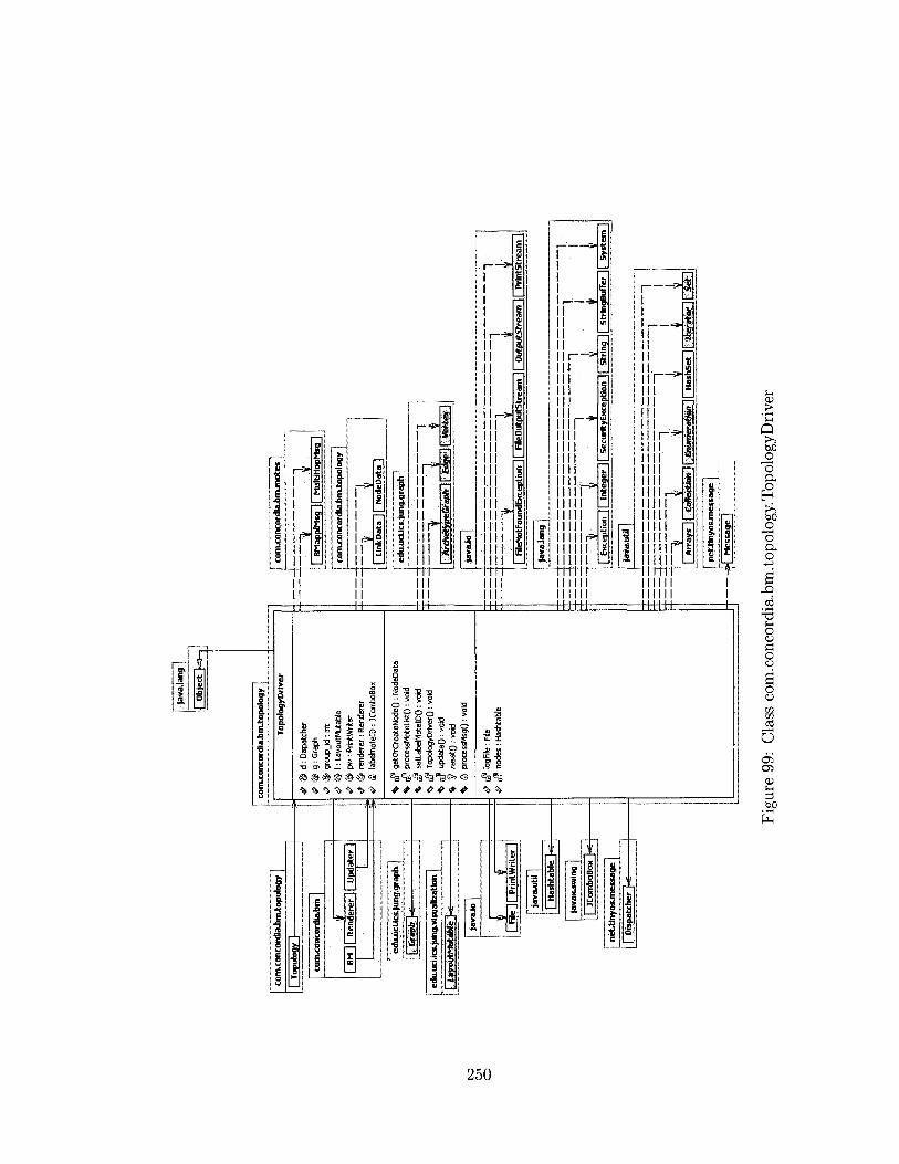
java
.lang
] O
bjec
t fo
—|
to
Or
O
com
.con
cord
ia.b
m.to
polo
gy j
Topo
logy
1
com
xonc
ordi
aJm
i
BM |
| R
ende
rer
[j U
pdat
er
ediU
icU
cs.ju
rig.g
rapb
edu.
ucuc
s.ji
ing>
visu
aIiz
atio
n
layw
XMt&
iiSte
) java
Jo
File
Pr
intW
riter
java
.util
j
[ I
Has
htab
le |
java
x.sw
ingj
JCom
boBo
x I
nett
fnyo
s.m
essa
ge
Dis
patc
her
h^
-
com
.con
cord
ia.b
m.to
polo
gy
Topo
logy
Driv
er
# d:
Disp
atch
er
g : G
raph
T$
gro
upJd
: int
$
I: L
ayou
tMut
able
pw
: Pr
intW
riter
&
re
nder
er:
Ren
dere
r St
lab
elm
otel
D: J
Com
boBo
x
^ dp
get
OrC
reat
eNod
e():
Nod
eDat
a %
$
proc
essM
otel
ist(
): vo
id
%
setL
abeI
Mot
eID
(): v
oid
<> $
To
polo
gyD
river
(): v
oid
^ cf
up
date
(): v
oid
%
f re
set(
) : v
oid
%
i2 p
roce
ssM
sgQ
: v
oid
^ cf
log
File
; Fi
le
&
i§ n
odes
: H
asht
able
com
.con
cord
fa.b
mjn
otes
If B
Map
plM
sgll
Mul
tiHop
Msg
|
com
.con
cord
ia.b
m.to
polo
gy ]
1 Li
nkD
atal
l N
odeD
ata]
edu.
uci.i
cs.ju
ng.g
raph
i
3.
"1
INifeM
ilftNSftW
wi Iv-jsa
MNKJ
h-.ji&
atie--
java
.io
IJL
File
Not
Foun
dExc
eptio
n H
File
Out
putS
trea
m 1
j Out
putS
trea
m [
fPri
ntS
trea
m
java
Jang
. 1
? i
v •
v Ex
cept
iofT
l 1 I
nteg
er"]
1 Se
curit
yExc
eptio
n""]
| St
ring"
! 1
Strin
gBuf
fer
| ( Sy
stem
"]
java
.uti
l j
i ~i
n
I 1
"i '
y ^
y ^
y I
Arr
ays
|f C
a^lt
on
\\B
i>u
m**
tlo
n ||
Has
hSeF
ll /H
yata
f ||-
ne£.
tmyo
s.m
essa
ge i
Mes
sage
Figu
re 9
9: C
lass
com
.con
cord
ia.b
m.to
polo
gy.T
opol
ogyD
rive
r

to
Cn
com
.!
Wot
ftsB
rfcf
ae
Uar
tDet
ect
1
com
,ct>
fico
rdia
,bri
nt»m
otes
SMsp
plM
sfl
Mul
iHop
Msg
U
artD
etec
tCon
sts
Uar
tDet
ectM
sq
DB
Con
nect
ion
DBL
inkT
able
D
BR
eadi
ngTa
ble
DB
Upd
ateQ
uery
Figu
re 1
00:
gate
way
/ser
ver
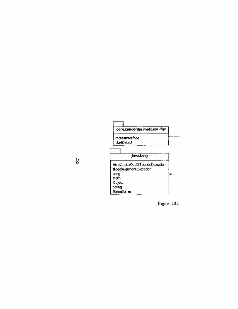
com.concordia.motesbndge
Moteslnterface UartDetect
javaJang
ArraylndexOutOfBoundsException IllegalArgumentException Long Math Object String StringBuffer
Figure 101

com.concordia.bm.motes
BMapplMsg MultiHopMsg UartDetectConsts UartDetectMsg
net.tinyos.message
LinkedMessage Message
Package com.concordia.bm.motes

to
cn
co
era
c 1-i
CD
l—'
O
to O
p'
CO CD
O
o o o t3
o o i-i &
p"
a"
3 td
p •o
>11
cn
TO

net t tnyoMnessage
Linked Message {subclasses ° 2}
c omxoncor tflaJwrurwrtes
# J3 AM_TYPE : tnt * # DEFAUIT_MES5AG£_SIZE : int
% $ etementSttejtotaQ : Int * # etement5ire6&s_data0 : int * dp get_data(): short{] % tf getjdO : short * $ get.origmaddrO : Int % J 5 get_origmseqno() : short * df get_seqno{): short % dP get_sourceaddr(): int * $ get.uK) : short * df getElement_data(): short * getStrtng_data(): String ^ isArrayjdataQ : boolean % if IsArrayJdQ: boolean % J 5 lsArray_orlginaddr(): boolean % J" tsArrayjxtqriseqnoO : boolean * t*p lsArray_seqno(): boolean ^ $ feArray_sourceaddr(): boolean * ^ isArray_tB(): boolean % •£> lsSioned_data(): boolean * $ isSiqned JdQ: boolean % is5igned_ortginaddrO: boolean ^ i 3 is5igned_ortqlnseqno(): boolean % is5lgned_seqno0: boolean % if? i»Signed_sourceaddr(): boolean % $ isSignedJtK): boolean * sP MuftHopMsgO: void ^ sJ3 MultHopMsgO: void ^ $ MuftlHopMsgO: void ^ Mu&iHopMsgO: void ^ $ MultWopMsgO: void <> MultWopMsgO i void * iP MultiHopMsgO : void
MultiHopMsgO : void % numDimensionsjtetaO: int * ,iJ numEtements_data(): int ^ ciP numElentents.dataO • int * tf offset _dataO i mt * J* offset JdQ f Int % J5 offset _orlgmeddr(): mt \ ujf* offset_ori^nseqrvj(); Int * if offset_seqno(); tnt \ of5 offset_sourceaddrO: Int % offset _ttt(): Int % liP offsetBits_data() : int % $ offsetKsjdO : int % ClP offsetBts.originacWrO : int % aP offset8its_originseqno0: int * cf offsetats.seqnoO : mt % i P offsetBfts_sourceaddr(): int % if offsetBfts_tti(): W * tip set_data(): void % $ set _id(); vend ^ set_originaddr(): void \ set.originseqnoO: void * $ set_seqno(>: void V riP set_sourceaddr(): void * 0? set.ttt(); vcid * $ settlement jtetaO; void V i# setString.dataO: void % $ size JdQ:*t \ ttP sea_ori n3<Jdr(): mt ^ $ size.originseqnoO: int % $ soe.seqnoO: int \ iiP st2e_sourceaddr(): int * rj? sfeeJtlO : int \ $ stents _id<) : int ^ rjp skeKts_arighaddfO: int % $ sizeftts_orighseqno(): int ^ J 3 steeBts_seqno(): mt % J* sizeBit5_sotffceaddr(): mt \ sfeeKts JtK) : Int % J 3 toStringO: String * $ totalSlze.dat a(): Int + J 3 totaSi2eBits_dataO : int
• H Message |
"> 1 "i . I * I 11 Long 11 Math | | String |1 StringBuffer I
nebtlnyosjnessage
Figure 103: Class com.concordia.bm.motes.MultiHopMsg
254

java.lang
Object
com.concordia.bm.motes
UartDetectConsts
# J 8 AM_UARTDETECTMSG : byte # dP UARTDETECT_KEEPALIVE i byte # J 8 UARTDETECT_PQLL : short # dP UARTDETECT_REQUE5T : byte # dP UARTDETECT_RE5PON5E : byte
Figure 104: Class com.concordia.bm.motes.UartDetectConsts
255
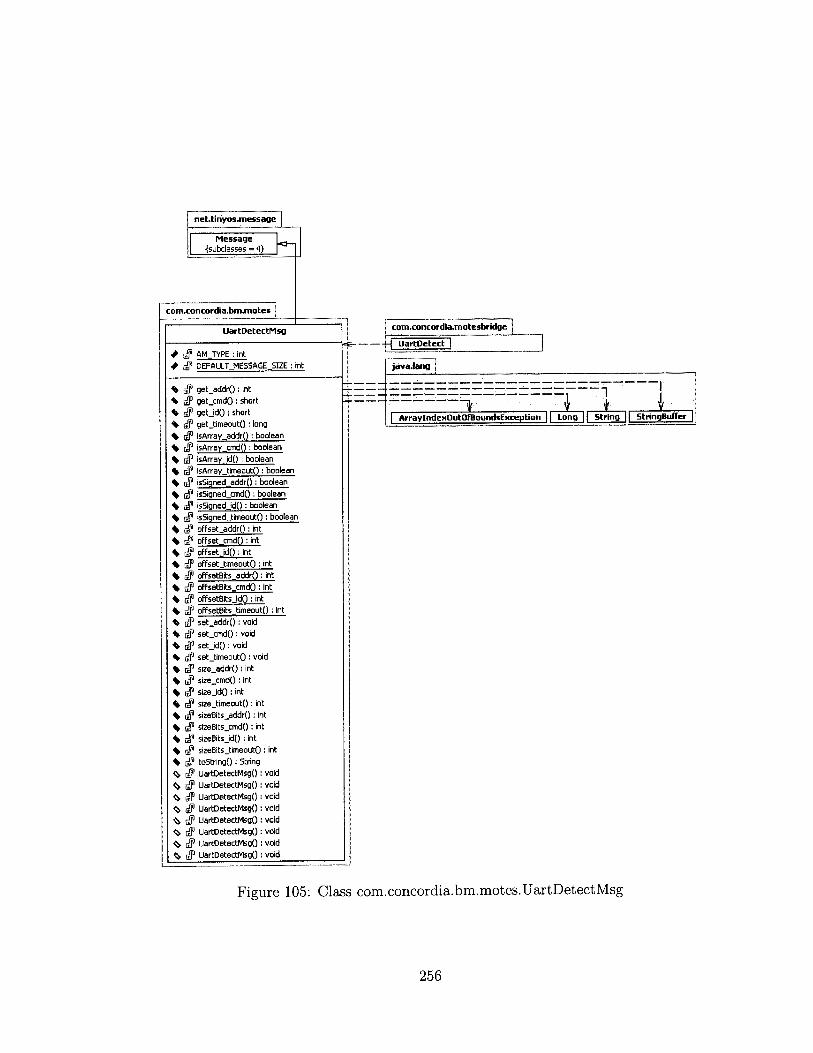
net.tinyos.message
Message •{subclasses = 1}
com.concordia.bm.motes
UartDetectMsg
4 d P AM_TYPE : int 4 d P DEFAULT_ME5SAGE_5IZE : int
V i f ge t_addr ( ) : int * d P ge t_cmdO: short * d P g e t j d ( ) i short
V EtP ge t J imeou tQ : long ^ d P isArray_addrQ; boolean
d P isArray_cmdQ: boolean d P isArray_id(): boolean dP isArray_timeout(): boolean dP isSigned_addr(): boolean J® isSigned_cmdQ: boolean dp isSignedJdQ: boolean d P is5igned_timeout(); boolean
% * * %
% * i f o f fse t_addr( ) : int \ i f of fse t_cmdQ: int
' offset_id() : int 1 offset_t imeout() : int ' offsetBits_addr(): int
dP offsetBits .cmdQ: int dP of fse tBi t sJdQ: int dP offsetBitsJimeoutQ : int dP se t_addr ( ) : void J 9 se t_cmd(): void dP s e t j d ( ) : void d p set_t imeout() : void t f s ize_addrO: int d P size_cmd(): int d P s i z e J d O : int d P s i zeJ imeoutO: int d P sizeBits_addrO : int d P sizeBits_cmd(): int d p sizeBitsJdO : int d P sizeBits_timeout(): int d p toStringO: String d P UartDetectMsgO : void d P UartDetectMsgO : void d p UartDetectMsgO ! void d P UartDetectMsgO: void
^ d P UartDetectMsgO : void ^ d p UartDetectMsgO : void ^ d p UartDetectMsgO : void
d P UartDetectMsgO i void
com.concordia.motesbridge
- - I l lartPetect
java.lang
'Jl 1 ArraylndexOutOfBoundsExceptionll Long || String || StringBuffer
Figure 105: Class com.concordia.bm.motes.UartDetectMsg
256

com.concordia.motesbridge
ClientsHandler MotesBridge Moteslnterface UartDetect
java.lang
Exception Integer InterruptedException Object RtmaWe RuntimeException String StringBuffer System Thread
java.util
Vector
net.tinyos.util
Messenger PrintStreamMessenger
Figure 106: Package com.concordia.motesbridge
257

com
.con
cord
ia.m
otes
brid
ge
Mot
esBr
idge
||
Mot
esln
terf
ace
java
.io
£ In
putS
trea
m
|| O
ulpu
tStr
eam
java
.lang
¥ -
¥ |
Strin
g ||
Thre
ad"!
java
.net
Sock
et
java
.lang
| O
bjec
t ~[<
a—
com
.con
cord
ia.m
otes
brid
ge
Clie
ntsH
andl
er
# is
: In
putS
tream
#
ml:
Mot
esln
terfa
ce
nam
e : S
tring
#
os :
Out
putS
tream
£S
mB
: M
otes
Brid
ge
ill m
essa
gehe
ader
leng
th :
int
S so
cket
: S
ocke
t §
thre
ad :
Thr
ead
5 IO
Exce
ptio
n
<5> J
3 Clie
ntsH
andl
er():
voi
d %
RFP
join
(): v
oid
%
J3 run
(): v
oid
%
dp s
hutd
ownd
ient
(): v
oid
\ $
star
tdie
nt():
voi
d %
J®
writ
ePac
kets
Q :
voi
d %
f
read
From
Sock
etQ
: b
yte[
] %
f
read
N()
: by
te[]
%
$ w
riteT
oSoc
ketQ
: bo
olea
n %
§
initQ
: v
oid
^ ©
re
adPa
cket
sQ :
voi
d
com
.con
cord
ia.m
otes
brid
ge
1 M
otes
lnte
rfac
e
java
.io
java
.lang
'JL
JL
Inte
rrup
tedE
xcep
tion
|| St
ringB
uffe
r
java
.net
5 H
In
etA
ddre
ss
Figu
re 1
07:
Cla
ss
com
.con
cord
ia.m
otes
brid
ge.C
lien
tsH
andl
er

com
.con
cord
ia.m
otes
brid
ge
Clie
ntsH
andl
er
Mot
esln
terf
ace
Uar
tDet
ect
fava
Jo j
java
.lang
Stri
ng
HH
to Cn
CO
com
xonc
ordi
ajri
otes
brid
ge
Mot
es8r
idge
# dr
GRO
UPI
D :
int
# dP
NOD
EFIL
E : S
tring
&
dP
ser
verP
ort:
int
+ cf
st
artT
ime
: lon
g #
^ pw
: P
rintW
riter
#
5J d
ispla
yHel
p : b
oole
an
# &
gui
Mod
e : b
oole
an
# S
ml:
Mot
esln
terf
ace
# S
nClie
nts
: int
#
S nM
essa
gesR
eadF
rom
Mot
es :
int
3 nM
essa
gesW
ritte
nToM
otes
: in
t #
Q
nPac
kets
Rec
ieve
dFro
mC
lient
s :
frit
# £2
nPa
cket
sSen
tTod
ient
s : i
nt
# S
stat
usLi
ne :
boo
lean
#
© u
artD
etec
t: U
artD
etec
t
%
dp c
lear
Cou
ntsO
: v
oid
^ dP
dec
rem
ent C
lient
s():
voi
d %
dP
inc
rem
entC
fien
ts()
: voi
d %
df
ina
emen
tMes
sage
sRea
dFro
mM
otes
()'
void
^
dP i
ncre
men
tMes
sage
sWrit
tenT
oMot
esO
• v
oid
% dP
in
crem
entP
acte
tsR
ecie
vedF
rom
Clie
ntsO
: v
oid
^ dP
inc
rem
entP
acke
ts5e
ntTo
Clie
nts(
): vo
id
^ dP
iis
tenS
erve
rSto
pped
():
void
^
dP
mai
nQ :
voi
d ^
dp M
otes
Brid
geQ
: vo
id
%
dp p
rint
mes
sage
Q :
voi
d %
dp
sta
rtSe
rver
O :
voi
d %
dp
sto
pSer
ver(
): v
oid
% dP
up
date
Cou
nter
s():
voi
d ^
dear
Cou
nter
sLin
eO t
voi
d §
prin
tHel
pO :
voi
d ^
Qs P
roce
ssC
omm
andL
ineA
rgs(
): vo
id
java
io
T i f
! |
Buf
fere
dOut
putS
trea
m 1
O
utpu
tStr
ea/n
j
Pri
ntst
ream
|
java
Jang
-1
"T 1
'1 I JL
"1 I 1.
Exc
epti
on! 1
Int
eger
j |
R
Win
abfe
j Ist
ring
Buf
fer
|| S
yste
m |
| Th
read
net.t
inyo
s.m
essa
ge
Mot
eIF~
Figu
re 1
08:
Cla
ss c
om.c
onco
rdia
.mot
esbr
idge
.Clie
ntsH
andl
er

to
o>
o
java
Jang
I O
bjec
t ~
1<
I-
com
xonc
ordl
ajno
tesb
ridg
e
net.t
faiy
os.m
essa
ge
Mes
sage
lisle
ner
{subd
assei
3>
n .J
Mot
esln
terf
ace
grou
pJd
: int
0
th:
Thre
ad
iS c
lient
s: V
ecto
r '
S d
: Dis
patc
her
• &
m
B :
Mot
esB
ridge
1 $
m
ote
: Mot
elF
• $
pack
etam
type
: in
t •
<2 p
acke
tbas
eoff
set:
int
' S
pack
etda
tale
ngth
: in
t '
pare
rrta
mty
pe :
int
pare
ntba
seof
fset
: int
'
pare
ntda
tale
ngth
: in
t •
iS s
erve
rSoc
ket:
Serv
erSo
cket
=H
Clie
ntsH
andl
er !
* dP
get
Mes
sage
Dat
a():
byt
eG
^ J9 g
etM
otel
FQ :
Mot
elF
%
J3 m
essa
geR
ecei
ved(
): vo
id
^ qJP
Mot
esIn
terf
ace(
): v
oid
^ dp
rem
oveC
!ien
t():
void
^
dP
runQ
: vo
id
^ dP
$en
dMes
sage
():
void
^
J3 sh
utdo
wn(
): v
oid
%
&
dean
upQ
: v
oid
%
t2 s
hutd
ownA
BCfie
ntsO
: vo
id
com.co
ncGrdia
Jimjrnp
fces
|
"1
1 BM
applM
sjll M
ultlHopM
sg 1
co
m.c
onco
rdia
jnot
esbr
idge
'JL
"1
IOEx
cept
ion
11 P
rint
Str
eam
java
Jang
1L
™I
i 1
Exce
ptio
n H
In
terr
upte
dExc
eptio
n ||
Str
ing]
[ St
ringB
uffe
r |j
Sys
tem
^
java
.net
j
3H
Sock
et 1
neLtiny
os.me
ssage
i i
Pis
patc
hlFl
l M
essa
ge
net.t
inyo
s.ut
il
Mes
seng
er
| j
Prin
tStr
eam
Mes
seng
er 1
Figu
re 1
09:
Cla
ss c
om.c
onco
rdia
.mot
esbr
idge
.Clie
ntsH
andl
er

ts5 Oi
Figu
re 1
10:
Cla
ss c
om.c
onco
rdia
.mot
esbr
idge
.Uar
tDet
ect