INSTITUTE OF PHYSICS PUBLISHING PHYSICS IN MEDICINE AND BIOLOGY

Phys. Med. Biol. 46 (2001) 63–76 www.iop.org/Journals/pb PII: S0031-9155(01)11343-6

Automated counting of mammalian cell colonies

Paul R Barber, Borivoj Vojnovic, Jane Kelly, Catherine R Mayes,Peter Boulton, Michael Woodcock and Michael C Joiner

Gray Laboratory Cancer Research Trust, PO Box 100, Mount Vernon Hospital, Northwood,Middlesex HA6 2JR, UK

E-mail: barber@graylab.ac.uk

Received 26 January 2000, in final form 27 June 2000

AbstractInvestigating the effect of low-dose radiation exposure on cells using assaysof colony-forming ability requires large cell samples to maintain statisticalaccuracy. Manually counting the resulting colonies is a laborious task inwhich consistent objectivity is hard to achieve. This is true especially withsome mammalian cell lines which form poorly defined or ‘fuzzy’ colonies,typified by glioma or fibroblast cell lines. A computer-vision-based automatedcolony counter is presented in this paper. It utilizes novel imaging and image-processing methods involving a modified form of the Hough transform. Theautomated counter is able to identify less-discrete cell colonies typical ofthese cell lines. The results of automated colony counting are compared withthose from four manual (human) colony counts for the cell lines HT29, A172,U118 and IN1265. The results from the automated counts fall well within thedistribution of the manual counts for all four cell lines with respect to survivingfraction (SF) versus dose curves, SF values at 2 Gy (SF2) and total area underthe SF curve (Dbar). From the variation in the counts, it is shown that theautomated counts are generally more consistent than the manual counts.

1. Introduction

Specialized clonogenic assays have made it possible to examine the response of mammaliancellular systems to radiation with sufficient accuracy to resolve changes in radiosensitivity atdoses much less than 1 Gy where cell survival approaches 100%. These accurate colony-forming assays rely on determining precisely the number of cells that are ‘at risk’ eitherby the use of a fluorescence-activated cell sorter (FACS) to plate an exact number of cells(Wouters and Skarsgard 1994, Short and Joiner 1998, Short et al 1999a, b) or microscopicscanning to identify an exact number of cells after plating (Marples and Joiner 1993, Spadingerand Palcic 1993). However, manual counting of the cell colonies from either type of assayremains tedious, time-consuming and resource-intensive, considering that high cell numbersare required to achieve acceptable statistical accuracy. In addition to this, manual counting canbe subjective and it has been observed that results can differ between counting personnel (seefor example Lumley et al (1997)). The development of a reliable automated colony counter

0031-9155/01/010063+14$30.00 © 2001 IOP Publishing Ltd Printed in the UK 63

64 P R Barber et al

would reduce the time and resources required to perform such clonogenic assays. Furthermore,automatic methods offer objectivity together with possibilities for greater throughput overextended periods. Combined, these factors allow greater statistical accuracy and minimize theerror between comparable experiments.

The concept of computer-aided colony counting is not new and has been implementedby other groups (Thielmann and Hagedorn 1985, Parry et al 1991, Wilson 1995, Mukherjeeet al 1995, Hoekstra et al 1998, Dobson et al 1999). Several authors have noted the problemsassociated with detecting colonies around the periphery of a culture flask and several haveresorted to masking this area to exclude it from processing. Counting colonies that merge intoone another has also proved to be problematic, and statistical corrections have been employedto reduce systematic errors (Thielmann and Hagedorn 1985). Approaches to overcome theproblems of merging and less-discrete or fuzzy colonies giving multiple counts have resulted intotal-colony-area based statistical counts (Mukherjee et al 1995). Image-processing algorithmsbased on grey-level thresholding have been previously applied to the colony counting problem.This technique alone is not able to disregard the flask edge nor is it suitable for less-discretecolonies. More sophisticated algorithms based on grey-level watersheds have also been triedbut these tend to be computationally intensive, and give rise to multiple counts when presentedwith fuzzy colonies.

Since cell colonies tend to have some affinity for areas around the flask edge it seemsunreasonable to exclude these areas, as a reduction in statistical accuracy will result. Mergedand fuzzy colonies should also be treated correctly, without the need for statistical correctionor estimation. This paper describes an automated colony counter that uses algorithms robustto the problems described above. Also presented is the evaluation of the automatic colonycounter against four manual counts from skilled personnel.

2. Materials and methods

The automated colony counter was tested with four cell types, HT29, A172, U118 and IN1265,and the automated results were compared with those of manual counts from four experiencedstaff at the Gray Laboratory.

2.1. Flask preparation

2.1.1. Cell culture. Cell lines HT29, A172 and U118 were obtained from the EuropeanCollection of Animal Cell Cultures (ECACC) and were derived originally from a gradeI primary human colon adenocarcinoma, human glioblastoma and grade III astrocytoma–glioblastoma respectively. The IN1265 was supplied by Dr J Darling, Institute of Neurology,London, UK and was derived originally from a primary human glioma. All cells weremaintained in monolayer culture in vitro in Eagle’s minimum essential medium with Earles salts(Sigma-Aldrich Co. Ltd, UK) supplemented with 10% foetal calf serum, 2 mM L-Glutamine,sodium bicarbonate, 1 mM sodium pyruvate, 50 IU ml−1 penicillin and 50 µg ml−1

streptomycin. All cells were grown in an atmosphere of 90% N2, 5% CO2, 5% O2 andpassaged routinely once a week using a calcium-free salt solution containing 0.05% trypsinand 0.02% EDTA.

2.1.2. Cell sorting. Cells were sorted using a FACSVantage cell sorter in conjunctionwith CellQuest software (Becton-Dickinson, San Jose, CA). Cells were characterizedbased on their forward-scatter fluorescence (cell ‘size’) and side-scatter fluorescence (cell‘granularity’) and the desired population gated and sorted into T25 tissue-culture flasks (Greiner

Automated colony counting 65

Labortechnik, UK) each containing 5 ml of pre-warmed, pre-gassed culture medium. Thenumber of cells actually deflected (sorted) was recorded flask by flask and used to calculatesubsequent surviving fractions. Following cell sorting, flasks were returned to the incubatorfor at least 1 h to allow cells to attach to the growth surface.

2.1.3. Irradiation. Once attached, the cells were irradiated with x-rays generated by a Pantakunit operating at 240 kVp. Filtration of 0.25 mm Cu + 1 mm Al gave an HVL of 1.3 mm Cuat a dose rate of 0.2–0.4 Gy min−1. This was chosen to ensure exposure times of at least 15 sand hence accurate dosimetry in the low-dose range. Cell survival was determined after singledoses of up to 5 Gy but focusing on survival at doses less than 1 Gy. Following irradiation,flasks were returned to the incubator and left for 14 days to allow colony formation.

2.1.4. Staining of colonies. The colonies formed were stained using crystal violet (Sigma-Aldrich Co. Ltd, UK) at 20 mg ml−1 in 95% ethanol (Hayman, Essex, UK). The growth mediumwas first decanted and replaced with sufficient stain to overlay the bottom of the flask. Afterapproximately 20–30 min, the stain was removed by immersing the flasks three times underrunning cold water and the flasks were left to dry in air before colony counting proceeded.

2.1.5. Measurement of cell survival. Cell survival was measured according to the usualcriterion of 50 cells or more per colony (Puck and Marcus 1956) with either the automatedcolony counter or manually by the four observers using a Stuart Scientific colony counter.For these experiments the adherence of the automated counter to the 50 cell criterion wasdetermined by the user by appropriate parameter selection. Surviving fraction (SF) wascalculated by dividing the plating efficiency (PE) of irradiated cells by the PE of the cellpopulation of sham-irradiated cells.

2.2. Hardware

The hardware that we have developed incorporates a number of novel features which allowus to obtain high-quality images of the whole flask, including the flask corners. The systemconsisted of a monochrome camera with 1/3" format CCD with a wide-angle lens of 2.8 mmfocal length, which produced a field of view of 75 by 56 mm in the plane of the bottom ofthe culture flask. The bottom of the flask was at a distance of 62 mm from the lens flange(C-mount). We operated with the lens aperture fully opened (f/1.6) such that the depth offocus of the system was small compared with the height of the flask. The flask top surfacewas therefore significantly out of focus. Furthermore, the field of view in the plane of the topof the flask was only 24 × 16 mm, so the edges of the top of the flask did not appear in theimage. This arrangement significantly reduced image clutter and allowed a good view into thecorners of the flask. As can be seen in figure 1, the bottom edge of the flask was visible aroundthe outside of the image and colonies could be identified both inside and outside this border.

Standard culture flasks of type T25 with a flat bottom surface measuring 68×40 mm wereused in all experiments. These were located under the camera with a simple jig consistingof three locating screws and a spring. The jig ensured that the culture flask was always in areproducible position below the camera. Prior knowledge about the approximate position ofthe flask was used to aid the removal of flask structure in later image processing.

The flask was illuminated from below by an electroluminescent film (Pacel ‘blue-green’type) which provided extremely uniform illumination at a wavelength of around 520 nm, withbandwidth of approximately 80 nm. A white Perspex diffuser was used above the film to remove

66 P R Barber et al

Figure 1. A typical image captured by the automatic colony counter showing colonies of cell typeA172, many of which extend up the sides of the flask beyond the visible flask edge.

any slight imperfections in emission. This was protected by a 1 mm thick scratch-resistant,transparent plastic sheet (Edmunds type H43929). Illumination of this type gave optimalcontrast for imaging cells stained with crystal violet, matching its absorption spectrum. Thefilm was typically excited with a 150 V rms sine wave at 800 Hz, with the amplitude set to justproduce ‘peak white’ in the camera. This drive waveform was derived from the camera framerate (25 Hz) and phase-locked to it to ensure short- and long-term illumination stability.

Although the illumination was extremely uniform, the use of a wide-angle lens resultedin an apparent fall-off of illumination near the image edges, and gave rise to an effect similarto vignetting. This, however, could be easily removed with software where necessary. Atypical image captured by the CCD camera is shown in figure 1. The imaging arrangement isshown in figure 2, where the close proximity of the illumination, flask and lens can be seen.External sources of light were excluded with a simple curtain shield.

The images were captured into the memory of a 450 MHz personal computer (PC) witha National Instruments (NI) IMAQ PCI-1408 image-capture board. The image was capturedat a spatial resolution of 768 by 576 pixels and at an intensity resolution of 8 bits (256 levels),processed as a rectangular grid of square pixels.

2.3. Software

The software for the user interface and image processing was written in the C programminglanguage. In all cases of image capture, 10 images were stored and averaged to reduce camera

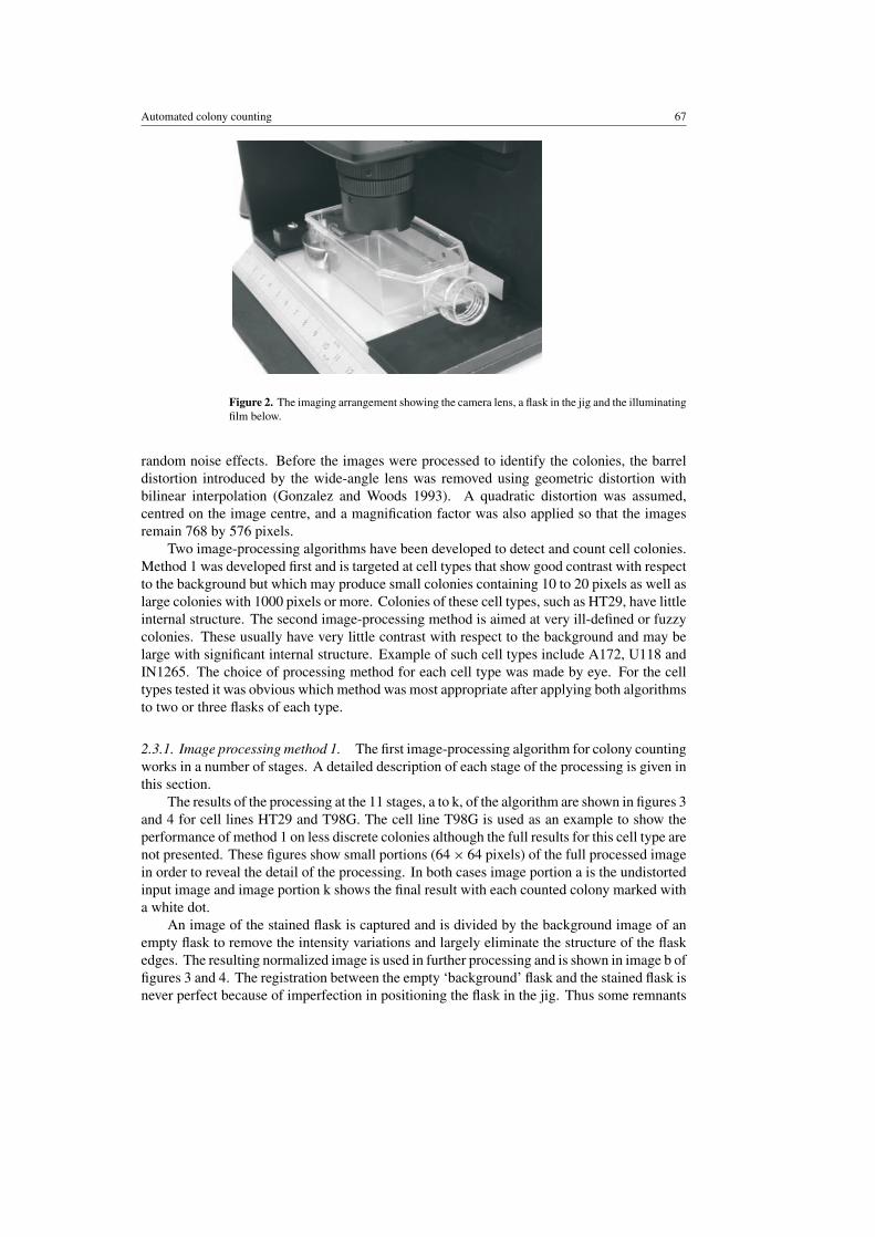
Automated colony counting 67

Figure 2. The imaging arrangement showing the camera lens, a flask in the jig and the illuminatingfilm below.

random noise effects. Before the images were processed to identify the colonies, the barreldistortion introduced by the wide-angle lens was removed using geometric distortion withbilinear interpolation (Gonzalez and Woods 1993). A quadratic distortion was assumed,centred on the image centre, and a magnification factor was also applied so that the imagesremain 768 by 576 pixels.

Two image-processing algorithms have been developed to detect and count cell colonies.Method 1 was developed first and is targeted at cell types that show good contrast with respectto the background but which may produce small colonies containing 10 to 20 pixels as well aslarge colonies with 1000 pixels or more. Colonies of these cell types, such as HT29, have littleinternal structure. The second image-processing method is aimed at very ill-defined or fuzzycolonies. These usually have very little contrast with respect to the background and may belarge with significant internal structure. Example of such cell types include A172, U118 andIN1265. The choice of processing method for each cell type was made by eye. For the celltypes tested it was obvious which method was most appropriate after applying both algorithmsto two or three flasks of each type.

2.3.1. Image processing method 1. The first image-processing algorithm for colony countingworks in a number of stages. A detailed description of each stage of the processing is given inthis section.

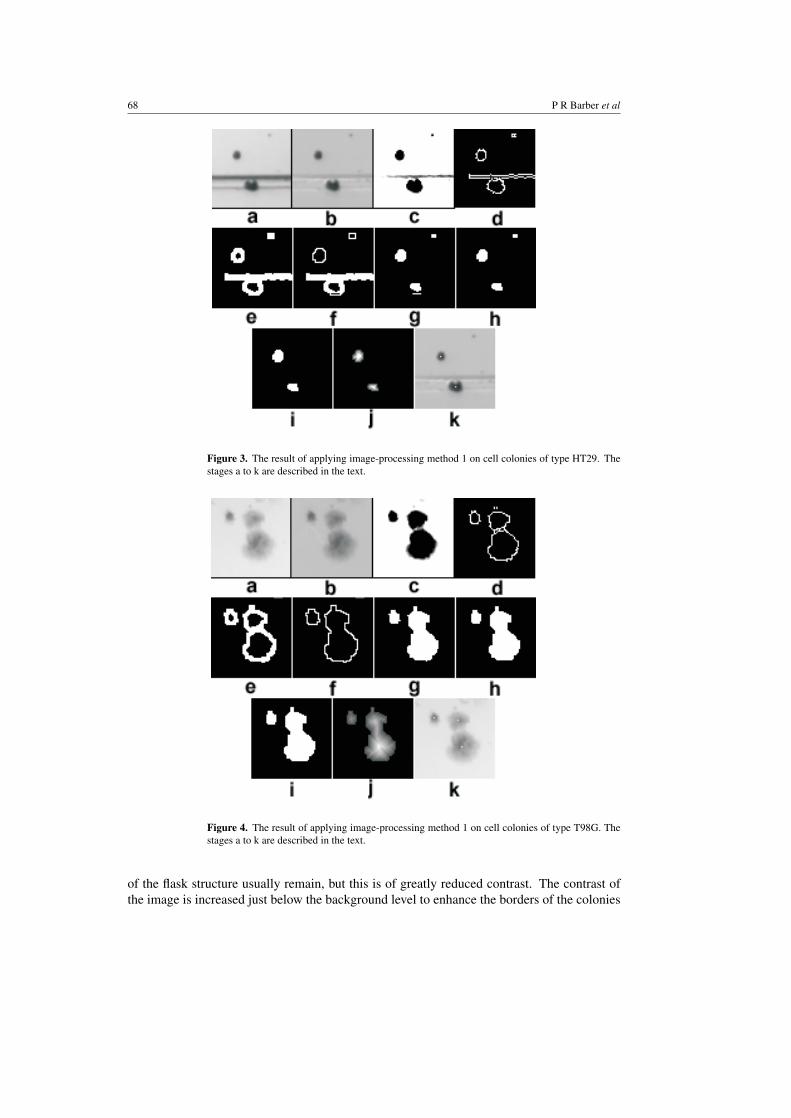
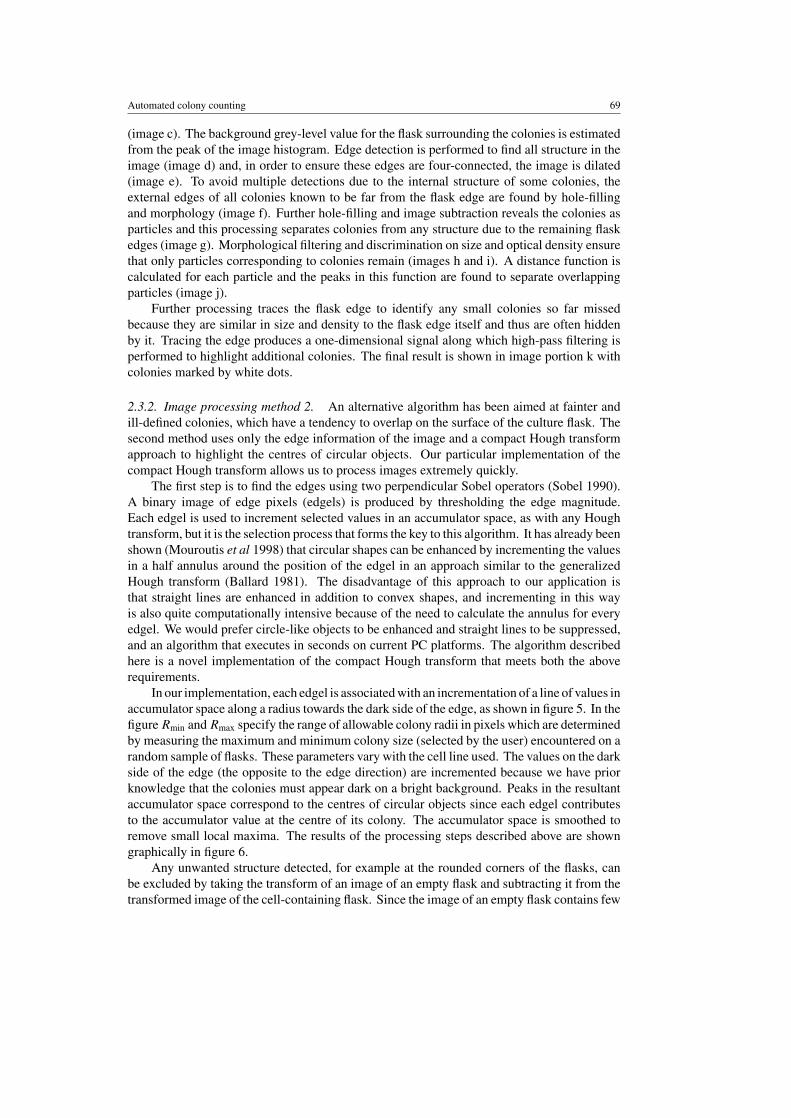
The results of the processing at the 11 stages, a to k, of the algorithm are shown in figures 3and 4 for cell lines HT29 and T98G. The cell line T98G is used as an example to show theperformance of method 1 on less discrete colonies although the full results for this cell type arenot presented. These figures show small portions (64 × 64 pixels) of the full processed imagein order to reveal the detail of the processing. In both cases image portion a is the undistortedinput image and image portion k shows the final result with each counted colony marked witha white dot.

An image of the stained flask is captured and is divided by the background image of anempty flask to remove the intensity variations and largely eliminate the structure of the flaskedges. The resulting normalized image is used in further processing and is shown in image b offigures 3 and 4. The registration between the empty ‘background’ flask and the stained flask isnever perfect because of imperfection in positioning the flask in the jig. Thus some remnants

68 P R Barber et al

Figure 3. The result of applying image-processing method 1 on cell colonies of type HT29. Thestages a to k are described in the text.

Figure 4. The result of applying image-processing method 1 on cell colonies of type T98G. Thestages a to k are described in the text.

of the flask structure usually remain, but this is of greatly reduced contrast. The contrast ofthe image is increased just below the background level to enhance the borders of the colonies

Automated colony counting 69

(image c). The background grey-level value for the flask surrounding the colonies is estimatedfrom the peak of the image histogram. Edge detection is performed to find all structure in theimage (image d) and, in order to ensure these edges are four-connected, the image is dilated(image e). To avoid multiple detections due to the internal structure of some colonies, theexternal edges of all colonies known to be far from the flask edge are found by hole-fillingand morphology (image f). Further hole-filling and image subtraction reveals the colonies asparticles and this processing separates colonies from any structure due to the remaining flaskedges (image g). Morphological filtering and discrimination on size and optical density ensurethat only particles corresponding to colonies remain (images h and i). A distance function iscalculated for each particle and the peaks in this function are found to separate overlappingparticles (image j).

Further processing traces the flask edge to identify any small colonies so far missedbecause they are similar in size and density to the flask edge itself and thus are often hiddenby it. Tracing the edge produces a one-dimensional signal along which high-pass filtering isperformed to highlight additional colonies. The final result is shown in image portion k withcolonies marked by white dots.

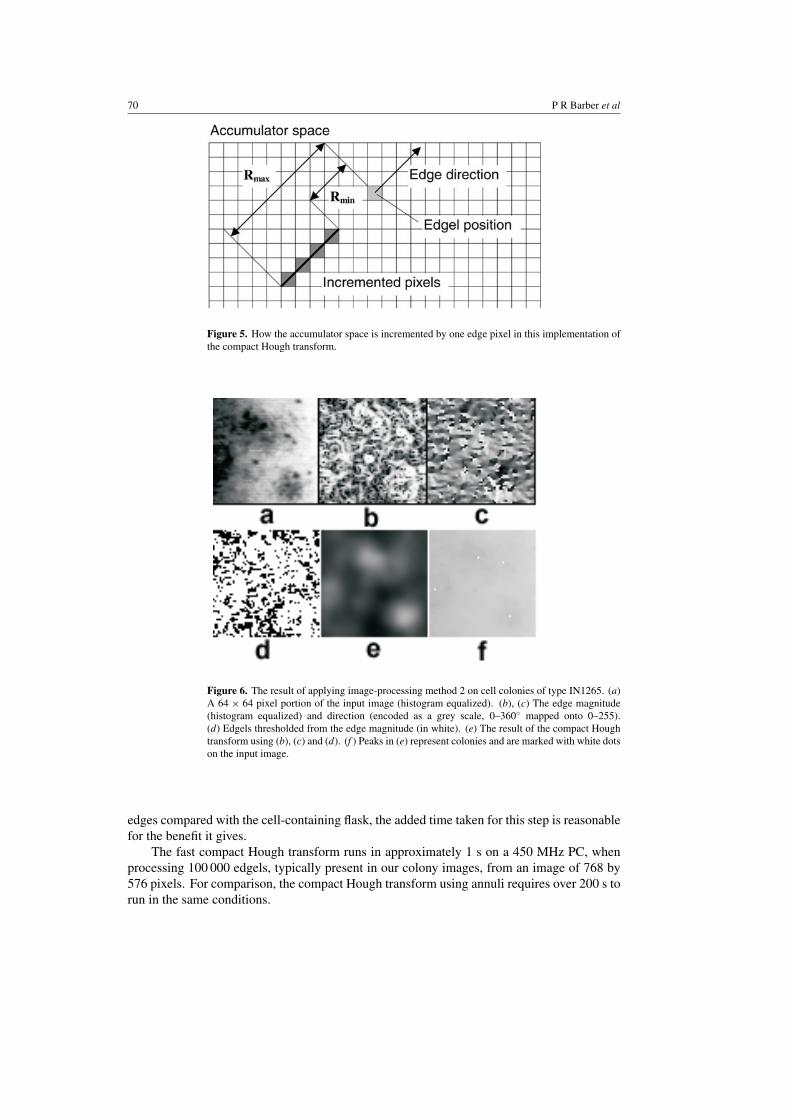
2.3.2. Image processing method 2. An alternative algorithm has been aimed at fainter andill-defined colonies, which have a tendency to overlap on the surface of the culture flask. Thesecond method uses only the edge information of the image and a compact Hough transformapproach to highlight the centres of circular objects. Our particular implementation of thecompact Hough transform allows us to process images extremely quickly.

The first step is to find the edges using two perpendicular Sobel operators (Sobel 1990).A binary image of edge pixels (edgels) is produced by thresholding the edge magnitude.Each edgel is used to increment selected values in an accumulator space, as with any Houghtransform, but it is the selection process that forms the key to this algorithm. It has already beenshown (Mouroutis et al 1998) that circular shapes can be enhanced by incrementing the valuesin a half annulus around the position of the edgel in an approach similar to the generalizedHough transform (Ballard 1981). The disadvantage of this approach to our application isthat straight lines are enhanced in addition to convex shapes, and incrementing in this wayis also quite computationally intensive because of the need to calculate the annulus for everyedgel. We would prefer circle-like objects to be enhanced and straight lines to be suppressed,and an algorithm that executes in seconds on current PC platforms. The algorithm describedhere is a novel implementation of the compact Hough transform that meets both the aboverequirements.

In our implementation, each edgel is associated with an incrementation of a line of values inaccumulator space along a radius towards the dark side of the edge, as shown in figure 5. In thefigure Rmin and Rmax specify the range of allowable colony radii in pixels which are determinedby measuring the maximum and minimum colony size (selected by the user) encountered on arandom sample of flasks. These parameters vary with the cell line used. The values on the darkside of the edge (the opposite to the edge direction) are incremented because we have priorknowledge that the colonies must appear dark on a bright background. Peaks in the resultantaccumulator space correspond to the centres of circular objects since each edgel contributesto the accumulator value at the centre of its colony. The accumulator space is smoothed toremove small local maxima. The results of the processing steps described above are showngraphically in figure 6.

Any unwanted structure detected, for example at the rounded corners of the flasks, canbe excluded by taking the transform of an image of an empty flask and subtracting it from thetransformed image of the cell-containing flask. Since the image of an empty flask contains few

70 P R Barber et al

Figure 5. How the accumulator space is incremented by one edge pixel in this implementation ofthe compact Hough transform.

Figure 6. The result of applying image-processing method 2 on cell colonies of type IN1265. (a)A 64 × 64 pixel portion of the input image (histogram equalized). (b), (c) The edge magnitude(histogram equalized) and direction (encoded as a grey scale, 0–360◦ mapped onto 0–255).(d) Edgels thresholded from the edge magnitude (in white). (e) The result of the compact Houghtransform using (b), (c) and (d). (f ) Peaks in (e) represent colonies and are marked with white dotson the input image.

edges compared with the cell-containing flask, the added time taken for this step is reasonablefor the benefit it gives.

The fast compact Hough transform runs in approximately 1 s on a 450 MHz PC, whenprocessing 100 000 edgels, typically present in our colony images, from an image of 768 by576 pixels. For comparison, the compact Hough transform using annuli requires over 200 s torun in the same conditions.

Automated colony counting 71

(a) (b)

(c) (d)

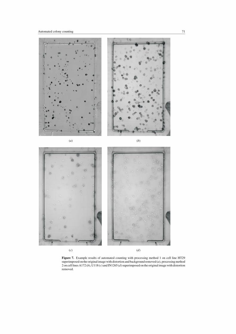
Figure 7. Example results of automated counting with processing method 1 on cell line HT29superimposed on the original image with distortion and background removed (a), processing method2 on cell lines A172 (b), U118 (c) and IN1265 (d) superimposed on the original image with distortionremoved.

72 P R Barber et al

Figure 8. Correlation of the mean automated colony counts versus mean manual colony countsfor HT29, A172, U118 and IN1265 cell lines. Each point represents the mean number of coloniescounted ± the standard error of the mean for each dose. Regression lines through the origin aredrawn and the correlation coefficients are shown in the bottom right-hand corner of each graph.

Figure 9. Plating efficiency (PE) for HT29, A172, U118 and IN1265 cell lines at four radiationdoses (0, 0.4, 2 and 5 Gy). Each bar represents the mean PE ± standard error of the mean.

Automated colony counting 73

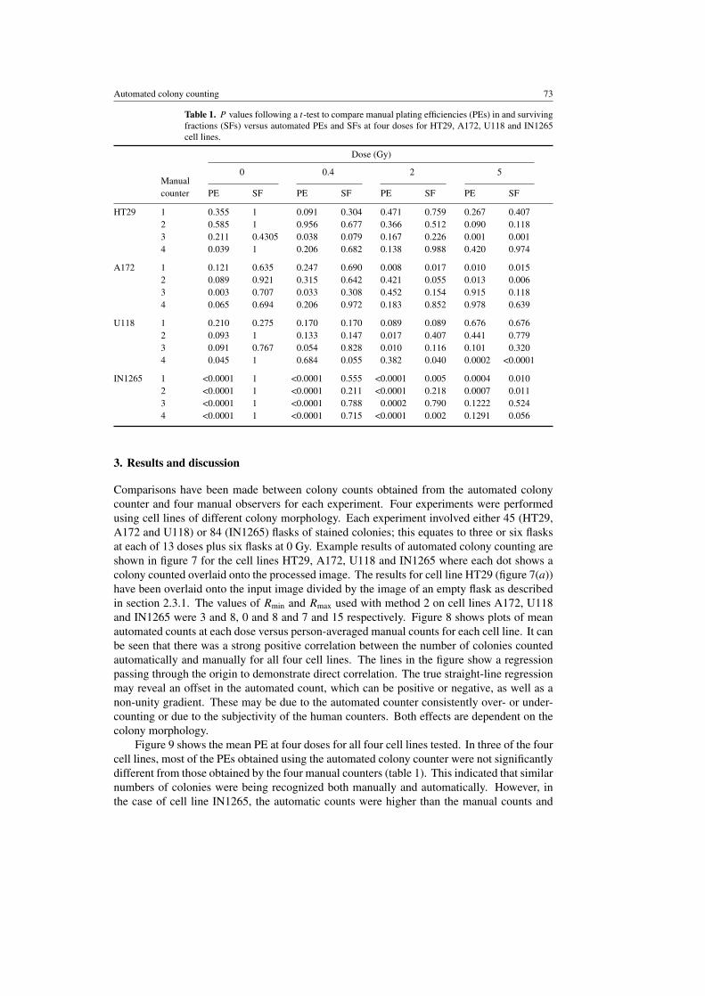
Table 1. P values following a t-test to compare manual plating efficiencies (PEs) in and survivingfractions (SFs) versus automated PEs and SFs at four doses for HT29, A172, U118 and IN1265cell lines.

Dose (Gy)

0 0.4 2 5Manualcounter PE SF PE SF PE SF PE SF

HT29 1 0.355 1 0.091 0.304 0.471 0.759 0.267 0.4072 0.585 1 0.956 0.677 0.366 0.512 0.090 0.1183 0.211 0.4305 0.038 0.079 0.167 0.226 0.001 0.0014 0.039 1 0.206 0.682 0.138 0.988 0.420 0.974

A172 1 0.121 0.635 0.247 0.690 0.008 0.017 0.010 0.0152 0.089 0.921 0.315 0.642 0.421 0.055 0.013 0.0063 0.003 0.707 0.033 0.308 0.452 0.154 0.915 0.1184 0.065 0.694 0.206 0.972 0.183 0.852 0.978 0.639

U118 1 0.210 0.275 0.170 0.170 0.089 0.089 0.676 0.6762 0.093 1 0.133 0.147 0.017 0.407 0.441 0.7793 0.091 0.767 0.054 0.828 0.010 0.116 0.101 0.3204 0.045 1 0.684 0.055 0.382 0.040 0.0002 <0.0001

IN1265 1 <0.0001 1 <0.0001 0.555 <0.0001 0.005 0.0004 0.0102 <0.0001 1 <0.0001 0.211 <0.0001 0.218 0.0007 0.0113 <0.0001 1 <0.0001 0.788 0.0002 0.790 0.1222 0.5244 <0.0001 1 <0.0001 0.715 <0.0001 0.002 0.1291 0.056

3. Results and discussion

Comparisons have been made between colony counts obtained from the automated colonycounter and four manual observers for each experiment. Four experiments were performedusing cell lines of different colony morphology. Each experiment involved either 45 (HT29,A172 and U118) or 84 (IN1265) flasks of stained colonies; this equates to three or six flasksat each of 13 doses plus six flasks at 0 Gy. Example results of automated colony counting areshown in figure 7 for the cell lines HT29, A172, U118 and IN1265 where each dot shows acolony counted overlaid onto the processed image. The results for cell line HT29 (figure 7(a))have been overlaid onto the input image divided by the image of an empty flask as describedin section 2.3.1. The values of Rmin and Rmax used with method 2 on cell lines A172, U118and IN1265 were 3 and 8, 0 and 8 and 7 and 15 respectively. Figure 8 shows plots of meanautomated counts at each dose versus person-averaged manual counts for each cell line. It canbe seen that there was a strong positive correlation between the number of colonies countedautomatically and manually for all four cell lines. The lines in the figure show a regressionpassing through the origin to demonstrate direct correlation. The true straight-line regressionmay reveal an offset in the automated count, which can be positive or negative, as well as anon-unity gradient. These may be due to the automated counter consistently over- or under-counting or due to the subjectivity of the human counters. Both effects are dependent on thecolony morphology.

Figure 9 shows the mean PE at four doses for all four cell lines tested. In three of the fourcell lines, most of the PEs obtained using the automated colony counter were not significantlydifferent from those obtained by the four manual counters (table 1). This indicated that similarnumbers of colonies were being recognized both manually and automatically. However, inthe case of cell line IN1265, the automatic counts were higher than the manual counts and

74 P R Barber et al

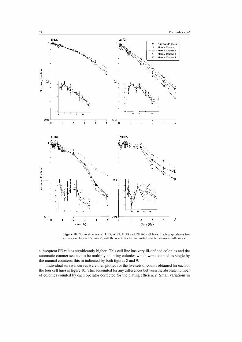
Figure 10. Survival curves of HT29, A172, U118 and IN1265 cell lines. Each graph shows fivecurves, one for each ‘counter’, with the results for the automated counter shown as full circles.

subsequent PE values significantly higher. This cell line has very ill-defined colonies and theautomatic counter seemed to be multiply counting colonies which were counted as single bythe manual counters; this in indicated by both figures 8 and 9.

Individual survival curves were then plotted for the five sets of counts obtained for each ofthe four cell lines in figure 10. This accounted for any differences between the absolute numberof colonies counted by each operator corrected for the plating efficiency. Small variations in

Automated colony counting 75

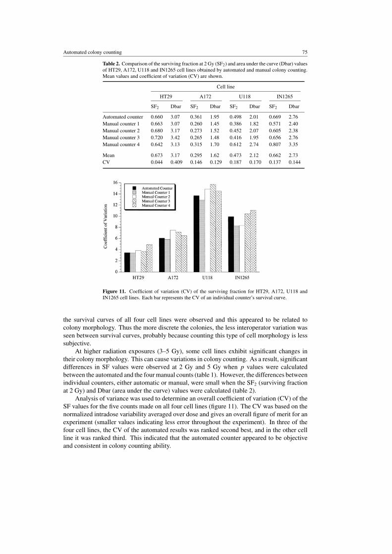
Table 2. Comparison of the surviving fraction at 2 Gy (SF2) and area under the curve (Dbar) valuesof HT29, A172, U118 and IN1265 cell lines obtained by automated and manual colony counting.Mean values and coefficient of variation (CV) are shown.

Cell line

HT29 A172 U118 IN1265

SF2 Dbar SF2 Dbar SF2 Dbar SF2 Dbar

Automated counter 0.660 3.07 0.361 1.95 0.498 2.01 0.669 2.76Manual counter 1 0.663 3.07 0.260 1.45 0.386 1.82 0.571 2.40Manual counter 2 0.680 3.17 0.273 1.52 0.452 2.07 0.605 2.38Manual counter 3 0.720 3.42 0.265 1.48 0.416 1.95 0.656 2.76Manual counter 4 0.642 3.13 0.315 1.70 0.612 2.74 0.807 3.35

Mean 0.673 3.17 0.295 1.62 0.473 2.12 0.662 2.73CV 0.044 0.409 0.146 0.129 0.187 0.170 0.137 0.144

Figure 11. Coefficient of variation (CV) of the surviving fraction for HT29, A172, U118 andIN1265 cell lines. Each bar represents the CV of an individual counter’s survival curve.

the survival curves of all four cell lines were observed and this appeared to be related tocolony morphology. Thus the more discrete the colonies, the less interoperator variation wasseen between survival curves, probably because counting this type of cell morphology is lesssubjective.

At higher radiation exposures (3–5 Gy), some cell lines exhibit significant changes intheir colony morphology. This can cause variations in colony counting. As a result, significantdifferences in SF values were observed at 2 Gy and 5 Gy when p values were calculatedbetween the automated and the four manual counts (table 1). However, the differences betweenindividual counters, either automatic or manual, were small when the SF2 (surviving fractionat 2 Gy) and Dbar (area under the curve) values were calculated (table 2).

Analysis of variance was used to determine an overall coefficient of variation (CV) of theSF values for the five counts made on all four cell lines (figure 11). The CV was based on thenormalized intradose variability averaged over dose and gives an overall figure of merit for anexperiment (smaller values indicating less error throughout the experiment). In three of thefour cell lines, the CV of the automated results was ranked second best, and in the other cellline it was ranked third. This indicated that the automated counter appeared to be objectiveand consistent in colony counting ability.

76 P R Barber et al

The results show that the automated colony counter is able to produce SF measurementsconsistent with manual counters for cell lines with colonies as ill-defined as those for IN1265.The effect of a non-unity gradient in figure 8 is evident in when calculating PE (see figure 9)which is more noticable with the IN1265 cell line. However, its effect is removed when SFand Dbar values are calculated.

Any counting offset in figure 8 will cause errors in the automatically derived SF and Dbarvalues, but we see from the CV results of figure 11 that its effect is not significantly larger thansimilar errors between the manual counts. Further work should be aimed at counting accuracyin order to reduce such errors but the problem of identifying a ‘gold standard’ by which tojudge performance will then become prevalent.

The average time to process flasks using the automated colony counter was approximately30 s per flask, including the time taken to manually load and unload the flask from the unit.

Acknowledgments

The financial support of the Cancer Research Campaign (CRC) is gratefully acknowledged(grant SP219510202). We thank Mr J Prentice and Mr R G Newman for help with constructionof the device described here and Mrs R J Locke for useful discussions during softwaredevelopment. We also thank Mr A Lawrence for assistance with development of user interfacecode.

References

Ballard D H 1981 Generalizing the Hough transform to detect arbitrary shapes Pattern Recognition 13 111–22Dobson K, Reading L and Scutt A 1999 A cost-effective method for the automatic quantitative analysis of fibroblastic

colony-forming units Calcified Tissue Int. 65 166–72Gonzalez R C and Woods R E 1993 Digital Image Processing (Reading, MA: Addison-Wesley) ch 5Hoekstra S J, Tarka D K, Kringle R O and Hincks J R 1998 Development of an automated bone marrow colony

counting system In Vitro Mol. Toxicol. 11 207–13Lumley M A, Burgess R, Billingham L J, McDonald D F and Milligan D W 1997 Colony counting is a major source

of variation in CFU-GM results between centres Br. J. Haematol. 97 481–4Marples B and Joiner M C 1993 Response of Chinese hamster V79 cells to low radiation doses: evidence of enhanced

sensitivity of the whole cell population Radiat. Res. 133 41–51Mouroutis T, Roberts S J and Bharath A A 1998 Robust cell nuclei segmentation using statistical modelling Bioimaging

6 79–91Mukherjee D P, Pal A, Eswara S and Majumder D D 1995 Bacterial colony counting using distance transform Int. J.

Bio-Med. Comput. 38 131–40Parry R L, Chin T W and Donahoe K 1991 Computer-aided cell colony counting BioTechniques 10 772–4Puck T T and Marcus P I 1956 Action of x-rays on mammalian cells J. Exp. Med. 103 653–66Short S C and Joiner M C 1998 Cellular response to low-dose irradiation Clin. Oncol. 10 73–7Short S C, Mayes C, Woodcock M, Johns H and Joiner M C 1999a Low dose hypersensitivity in the T98G human

glioblastoma cell line Int. J. Radiat. Biol. 75 847–55Short S C, Mitchell S A, Boulton P, Woodcock M and Joiner M C 1999b The response of human glioma cell lines to

low-dose radiation exposure Int. J. Radiat. Biol. 75 1341–8Sobel I 1990 An isotropic 3×3 image gradient operator Machine Vision for Three-Dimensional Scenes ed H Freeman

(New York: Academic) pp 376–9Spadinger I and Palcic B 1993 Cell survival measurements at low doses using an automated image cytometry device

Int. J. Radiat. Biol. 63 183–9Thielmann H W and Hagedorn R 1985 Evaluation of colony-forming ability experiments using normal and DNA

repair-deficient human fibroblast strains and an automatic colony counter Cytometry 6 130–6Wilson I G 1995 Use of the IUL Countermat automatic colony counter for spiral plated total viable counts Appl.

Environ. Microbiol. 61 3158–60Wouters B G and Skarsgard L D 1994 The response of a human tumour cell line to low radiation doses: evidence of

enhanced sensitivity Radiat. Res. 138 S76–S80