automated design of steel wide-flanged …...automated design of steel wide-flanged beam floor...
TRANSCRIPT
AUTOMATED DESIGN OF STEEL WIDE-FLANGED
BEAM FLOOR FRAMING SYSTEMS USING
A GENETIC ALGORITHM
by
Benjamin T. Shock
A thesis submitted to the Faculty of the Graduate School, Marquette University, in Partial Fulfillment of the Requirements for the Degree of Master of Science
Milwaukee, WI July 2003

ii
Preface
The design of steel floor framing systems involves an optimization problem. This
problem involves choosing the structural elements used to construct the system so that
strength, deflection, and performance constraints are met, while achieving the lowest cost
possible for the structure. Traditionally, the design would be completed by an engineer
using a trial-and-error, iterative procedure according to design specifications and guided
by the experience of the designer. This process can be lengthy and is not guaranteed to
yield an optimal solution to the problem.
A better design tool is seen in the use of a genetic algorithm-based program that
performs the design automatically. The genetic algorithm (GA) is a search technique
modeled after the principles of “survival of the fittest” and adaptation. The GA does not
explore every combination of discrete design variables, but rather uses a small population
of individual solutions that improve as they adapt to fitness parameters over the course of
30 to 40 generations. The GA is a fast and efficient way to solve the floor framing
problem which involves a large number of discrete design variables.
A genetic algorithm-based program will be developed and implemented. It will
have the ability to choose beam and girder sizes, deck and concrete slab characteristics,
shear connector configurations, and floor panel layout based on simple user input. This
user input involves floor panel dimensions as well as superimposed dead and live loading
conditions. An output file is prepared by the GA for the program user detailing relevant
data of least-cost solutions.

iii
Conclusions are made as to the influence of cost variations and floor panel
geometry ratios on the most-economical solution. Suggestions are presented for building
designers and researchers wishing to reduce the panel cost and improve vibration
performance. Recommendations for future applications of the GA are provided along
with suggestions for improving its performance.

iv
Acknowledgements
I would like to express my sincere appreciation to my thesis director, Dr. Christopher M.
Foley, for his guidance and support throughout this thesis effort. The idea for this project
came from Dr. Foley, as did much of the initial organization. I would also like to thank
my fellow graduate student, Christopher W. Erwin, for his assistance in the early stages
of developing the genetic algorithm. Christopher, along with Dr. Foley, completed many
of the time-consuming tasks involved with the start of the project. For their work on
these tasks, I am grateful.
I would like to thank Dr. Sriramulu Vinnakota for his assistance in reviewing this
thesis and for his role as an exceptional professor and graduate advisor. I would also like
to thank Dr. Stephen M. Heinrich for his instruction and guidance throughout my
graduate education. As well as being on my thesis committee, Dr. Heinrich was an
outstanding professor and a mentor to me in the graduate research field.
I would also like to express my appreciation to my mother, Ruth M. Shock, as
well as the rest of my family and friends for their help and support throughout this
project. I would like to dedicate this thesis effort to the memory of my late father,
Stephen E. Shock. His support and guidance led me to reach for and achieve my goals.

v
Table of Contents
1 Introduction ........................................................................................................... 1
1.1 Objective and Scope ..................................................................................... 1
1.2 Background and Literature Review .............................................................. 2
1.3 Problem Statement ........................................................................................ 5
1.4 Overview of Contents ................................................................................... 9
2 Genetic Algorithm Fundamentals ....................................................................... 11
2.1 Encoding the Chromosome ........................................................................... 12
2.2 Creating the Initial Population ...................................................................... 13
2.3 Evaluation of Fitness .................................................................................... 13
2.4 Crossover ...................................................................................................... 13
2.5 Mutation and Elitism .................................................................................... 14
2.6 Generational Looping ................................................................................... 14
3 Programming the GA in MATLAB ................................................................... 16
3.1 allChecks.m .................................................................................................. 16
3.2 crossover.m .................................................................................................. 24
3.3 decodeChromo.m ......................................................................................... 26
3.4 eliminate.m .................................................................................................. 58
3.5 executeGA.m .............................................................................................. 60
3.6 findFitness.m .............................................................................................. 70
3.7 floorVib.m .................................................................................................. 78
3.8 gather.m ...................................................................................................... 90
3.9 initialPopulation.m ..................................................................................... 91
3.10 master.m .................................................................................................... 93
3.11 maximin.m ................................................................................................ 97
3.12 moreCheck.m ............................................................................................ 104
vi
3.13 mutation.m ............................................................................................... 104
3.14 ranking.m .................................................................................................. 106
3.15 selection.m ................................................................................................ 110
3.16 vmCheck.m ............................................................................................... 112
4 Design Checks for Constraint Evaluation ........................................................ 115
4.1 Shear Force and Bending Moment Capacities
of the Composite Beam Section .................................................................. 115
4.2 Shear Force and Bending Moment Capacities
of the Composite Girder Section ................................................................ 130
4.3 Bending Moment Capacities of the Beam
and Girder During Construction ................................................................. 136
4.4 Deflection of the Composite Beam and the Composite Girder .................. 138
4.5 Deflection of the Beam and Girder During Construction .......................... 146
4.6 Unshored Clear Span of the Steel Deck During Construction ................... 153
4.7 Steel Deck Live Load Rating ..................................................................... 153
4.8 Floor Panel Acceleration due to Walking Excitation ................................ 159
5 Parameter Studies and Algorithm Performance ............................................. 161
5.1 Sensitivity to Fabrication and Concrete Costs ............................................ 161
5.2 Sensitivity to Floor Panel Dimensions ........................................................ 165
5.3 Algorithm Performance .............................................................................. 169
5.4 Multiple Objective Optimization ............................................................... 171
5.5 General Observations and Concluding Remarks ....................................... 173
6 Recommendations for Future Research ........................................................... 180
References ............................................................................................................... 184
vii
Appendix A: Full MATLAB code .......................................................................... 187
A.1 allChecks.m ................................................................................................ 188
A.2 crossover.m ................................................................................................ 190
A.3 decodeChromo.m ....................................................................................... 191
A.4 eliminate.m ................................................................................................ 201
A.5 executeGA.m for single- objective fitness ................................................. 202
A.6 executeGA.m for multi- objective fitness .................................................. 213
A.7 findFitness.m .............................................................................................. 224
A.8 floorVib.m .................................................................................................. 228
A.9 gather.m ...................................................................................................... 232
A.10 initialPopulation.m ................................................................................... 233
A.11 master.m ................................................................................................... 234
A.12 maxiMin.m ............................................................................................... 237
A.13 moreCheck.m ........................................................................................... 239
A.14 mutation.m ............................................................................................... 250
A.15 ranking ..................................................................................................... 255
A.16 selection ................................................................................................... 253
A.17 vmCheck .................................................................................................. 256
Appendix B: Girder Deflection Assumption .......................................................... 270
Appendix C: distance_up calculations ................................................................... 274

viii
List of Figures
Figure 1.1: Floor framing system with user input and output ............................. 6
Figure 2.1: Chromosomal representation (34 binary digits) ............................... 12
Figure 2.2: Single-Point Crossover ..................................................................... 14
Figure 3.1: Organization of the m-file, executeGA, for single-objective genetic algorithm with evaluation of floor panel acceleration at the end of the evolution ................................................................. 17
Figure 3.2: Organization of the m-file, executeGA, for single-objective genetic algorithm using floor panel acceleration as a penalty .......... 18
Figure 3.3: Organization of the m-file, executeGA, for multi-objective genetic algorithm using maximin fitness evaluation ........................ 19
Figure 3.4: Pseudo-code detailing arrays phiProd and phiProd2, which contain penalty values from strength and deflection checks ............ 24
Figure 3.5: Steps of the crossover sequence ................................................. 27
Figure 3.6: Pseudo-code illustrating the crossover procedure ...................... 27
Figure 3.7: Pseudo-code used for decoding chromosome information into integer values ........................................................ 28
Figure 3.8: Pseudo-code used for adding 1 to each integer value for consistent labeling ...................................................................... 28
Figure 3.9: MATLAB code used for importing girder properties ...................... 32
Figure 3.10: Description of the fifteen girder properties ...................................... 32
Figure 3.11: Pseudo-code used for importing deck and concrete slab properties ............................................................. 37
Figure 3.12: Descriptions of the thirty-five deck and concrete slab properties .... 38
Figure 3.13: Floor panel configurations ............................................................... 39
Figure 3.14: Pseudo-code used to decode the number of divisions per girder length .............................................. 39
ix
Figure 3.15: Pseudo-code describing a feasibility check for number of divisions per girder length ................................................................. 43
Figure 3.16: Pseudo-code for decoding the number of shear studs per half beam ................................................ 43
Figure 3.17: Pseudo-code used for the beam stud feasibility check ..................... 45
Figure 3.18: Beam stud transverse layout for example problem .......................... 46
Figure 3.19: Pseudo-code used to reduce the number of studs to the maximum number of beam studs ..................................................... 47
Figure 3.20: Pseudo-code used for checking the minimum number of shear connectors per half beam .................................................... 49
Figure 3.21: Pseudo-code used to increase the number of studs to the minimum number of studs ..................................................... 50
Figure 3.22: Pseudo-code used for decoding the number of shear connectors per half girder ....................................................... 50
Figure 3.23: Pseudo-code used in the calculation for maximum number of studs per half girder ........................................................ 55
Figure 3.24: Pseudo-code used in reducing the number of studs per half girder .................................................. 55
Figure 3.25: Pseudo-code used in calculating the minimum number of studs per half girder ........................................................ 57
Figure 3.26: Pseudo-code used to increase the number of studs per half girder ........................................................ 57
Figure 3.27: MATLAB code illustrating the eliminate function ................... 59
Figure 3.28: Organization of m-file, executeGA, for single-objective genetic algorithm with evaluation of floor panel acceleration at the end of the evolution ........................................... 65
Figure 3.29: Organization of m-file, executeGA, for single-objective genetic algorithm using floor panel acceleration as a penalty ......... 66
Figure 3.30: Organization of the m-file, executeGA, for multi-objective genetic algorithm using maximin fitness evaluation ........................ 67
Figure 3.31: Pseudo-code detailing an adjustment on the baysGene ................ 69
x
Figure 3.32: MATLAB code describing the gene repair sub-function ................. 70
Figure 3.33: Definition and source for variables used within findFitness ... 74
Figure 3.34: Pseudo-code used in calculating the volume of concrete required for each individual solution ................................................ 75
Figure 3.35: Pseudo-code used for the calculation of total panel cost .................. 76
Figure 3.36: Pseudo-code detailing the process for cost-based fitness evaluation ...................................................... 77
Figure 3.37: Pseudo-code detailing the process for maximin fitness evaluation ............................................................... 77
Figure 3.38: Descriptions of some of the variables used within floorVib ...... 87
Figure 3.39: Pseudo-code used for calculation of beam mode properties ............ 88
Figure 3.40: Pseudo-code used for calculation of girder mode properties ............ 89
Figure 3.41: Pseudo-code used for calculation of vibration parameters ................ 90
Figure 3.42: Pseudo-code used in the gather function ....................................... 92
Figure 3.43: Pseudo-code describing the creation of the initial population ........... 92
Figure 3.45: Plot showing the general shape of a Pareto front .............................. 101
Figure 3.46: Pseudo-code used for evaluation of maximin fitness ........................ 102
Figure 3.47: MATLAB plots demonstrating progress of maximin fitness function ................................................................... 103
Figure 3.48: Pseudo-code illustrating the mutation procedure .................................. 107
Figure 3.49: Fitness array for ranking function ................................................. 108
Figure 3.50: Pseudo-code used for the column sort procedure .............................. 108
Figure 3.51: Array with sorted fitness values ........................................................ 109
Figure 3.52: Pseudo-code loop showing how chromosomes are reordered by fitness ..................................................................... 109
Figure 3.53: Population Partitioning Selection ..................................................... 113
xi
Figure 3.54: Pseudo-code describing the selection process .................................. 113
Figure 4.1: Pseudo-code and definitions for shear and moment checks in the composite beam ........................................................... 124
Figure 4.2: Pseudo-code and definitions for shear and moment checks in the composite girder ................................................................................ 132
Figure 4.3: Pseudo-code for bending moment check in the beam during construction .................................................................. 139
Figure 4.4: Pseudo-code for bending moment check in the girder during construction ................................................................. 140
Figure 4.5: Pseudo-code for deflection check of the composite beam ................ 147
Figure 4.6: Pseudo-code for deflection check of the composite girder ................ 149
Figure 4.7: Pseudo-code for deflection check of the beam during construction .................................................................. 154
Figure 4.8: Pseudo-code for deflection check of the girder during construction ................................................................. 155
Figure 4.9: Pseudo-code for checking unshored clear span of the steel deck during construction ........................................................... 156
Figure 4.10: Pseudo-code for steel deck live load check ....................................... 158
Figure 4.11: Pseudo-code for floor panel acceleration check ................................ 160
Figure 5.9: Convergence Trajectory Plot For Design 1 ....................................... 170 Figure 5.10: Multiple Objective Plots For Generations 1 and 10 of Design 6 ...... 174 Figure 5.11: Multiple Objective Plots For Generations 20 and 30 ........................ 175 Figure 5.12: Multiple Objective Plot For Final Generation .................................. 176 Figure B.1: Three test cases used to evaluate the validity of a
girder deflection assumption ............................................................. 275
Figure C.1: Schematic of composite beam assembly showing steel wide-flange section, steel deck, and the transformed concrete section. ............... 279
xii
Figure C.2: Schematic of composite girder assembly showing steel wide-flange section, steel deck, and the transformed concrete section. ................ 281
List of Tables
Table 3.44: Material Costs ................................................................................... 94
Table 5.1: System information for Sections 5.1, 5.2, 5.4, 5.5 ........................... 162
Table 5.2: Unit Costs Associated with the Studies of Chapter 5 ...................... 162
Table 5.3: Results for the “most-fit” individual for each of ten evolutions (Design 1) ....................................................................... 163
Table 5.4: Results for the “most-fit” individual for each of ten evolutions (Design 2) ....................................................................... 163
Table 5.5: Results for the “most-fit” individual for each of ten evolutions (Design 3) ....................................................................... 164
Table 5.6: Alternate Floor Panel Configurations for Section 5.3 ...................... 166
Table 5.7: Results for the “most-fit” individual for each of ten evolutions (Design 4) ............................................................. 167
Table 5.8: Results for the “most-fit” individual for each of ten evolutions (Design 5) ............................................................. 167

1
Chapter 1
Introduction
A genetic algorithm-based program has been developed to produce solutions for a
discrete variable floor panel optimization problem. A least-cost solution is desired that
meets strength, deflection, and performance constraints. The genetic algorithm (GA) is a
search technique modeled after the principles of “survival of the fittest” and adaptation.
The GA does not explore every combination of discrete design variables, but uses a small
population of individual solutions that improve as they adapt to fitness definitions. The
GA is a fast and efficient way to produce solutions to problems involving a large number
of discrete design variables, such as the floor framing design considered.
1.1 Objective and Scope
It was desired to have the genetic algorithm written using the MATLAB software
package (Mathworks 2003). The GA should have the ability to choose beam and girder
sizes, steel deck and concrete slab characteristics, shear connector configurations, and
floor panel layout based on simple user input. This input should include bay width and
length, as well as superimposed dead load and live load conditions. The program should
make use of nearly all available wide-flange sections from the AISC (2001) section
database. The program should have multiple options for steel deck height as well as steel
thickness. Both light-weight and normal-weight concrete should be available in varying
slab thicknesses. Multiple shear connector layouts should be available. The GA should
be able to select from floor panel systems with multiple beam configurations.

2
The program should perform all necessary strength, deflection, and performance
checks according to relevant specifications. Upon completion, the algorithm should
provide an optimized steel floor frame design based on the prescribed loading conditions,
the design checks, and the floor panel geometry. Details of the design should be
provided in an output file which is made available to the program user.
The scope of the thesis will now be discussed. The genetic algorithm will be
developed as summarized in the objectives section. Its behavior will be analyzed. Test
runs will be made to study the influence of unit cost variations and different panel
dimension ratios on the most-fit solution obtained. Additionally, different methods used
for evaluating the fitness of the solutions will be studied.
1.2 Background and Literature Review
The genetic algorithm is based on the principles of “survival of the fittest” and
adaptation. The genetic algorithm establishes a population of individuals, or unique
solutions to the engineering problem, and seeks to create the individual that is “most fit.”
The genetic make-up of each individual is encoded through a series of binary digits, 1’s
and 0’s, which comprise a grouping known as a chromosome. The effectiveness of each
individual at solving the original problem is evaluated, and individuals are selected to
mate based on their “fitness.” A new population of individuals is created through
reproduction, which entails crossover (swapping of random genes), to be followed again
by an evaluation of fitness. A mutation operator is included in this process, which serves
to randomly alter digits in the binary string, in order to keep the search open to new areas
of the search space. The whole process is repeated for a desired number of generations,
usually 20 to 100, until optimum or near-optimum solutions are obtained. Highly “fit”

3
individuals should eventually populate the group, with this condition being referred to as
convergence of the genetic algorithm.
The GA does not test every possible combination of design variables, but rather
uses a search technique in an effort to randomly sample data points throughout the search
space. The GA is a flexible and efficient search strategy for dealing with large and
complex search spaces.
The genetic algorithm has been used to obtain optimal or near-optimal solutions for
many types of discrete variable structural design problems. The form of the GA that is
used today was developed by Holland (1975) and Goldberg (1989). The simple GA
structure that was developed has been adapted to work with many kinds of structural
design problems. Several of the more pertinent applications are described in the
following sections.
Nearly ten years ago, the authors of Koumousis et al. (1994) used a GA-based
program to select member cross-sections for a steel, trapezoidal roof truss. They
concluded that the genetic algorithm offered an effective method for solving complex
discrete optimization problems.
The authors of Huang et al. (1997) investigated the use of the GA to design not only
two-dimensional trusses, but also two-dimensional, multi-story steel frames. They
proposed three solution strategies for addressing this kind of discrete variable
optimization problem. They also offered strategies for mitigating the large CPU times
that had become common for GA solutions.
4
In the following years, increasingly more complex problems were being addressed
by researchers using the genetic algorithm. The authors of Pezeshk et al. (1999) used a
GA-based optimization procedure to design of a geometrically nonlinear steel framed
structure. The authors sought to investigate the influence of the P-∆ effects on the design
of the structure, which followed standard AISC-LRFD guidelines. The author in
Hayalioglu (2001) successfully used a GA-based optimum design procedure to select
member sizes in a ten-story, 130-member space frame. His example problem converged,
reaching a minimum weight for the structure, after 101 generations.
In recent years, researchers have further investigated the inner workings of the GA.
They have studied the role of differing selection, crossover, and mutation schemes, as
well as the effect of population size and fitness scaling. The author in Hayalioglu
(2001) concluded that population size plays an important role in achieving the minimum
weight in a reasonable amount of generations. The authors in Pezeshk et al. (2000)
proposed an improved adaptive crossover operator, which is capable of blending the best
characteristics from other crossover schemes.
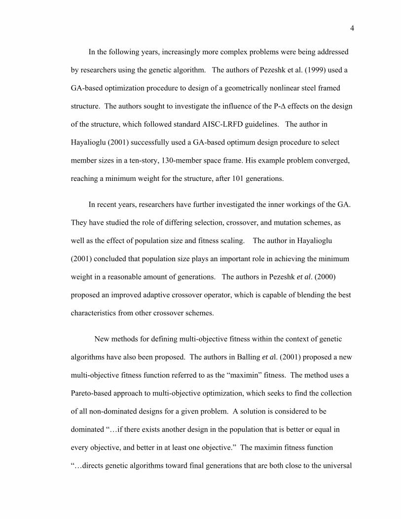
New methods for defining multi-objective fitness within the context of genetic
algorithms have also been proposed. The authors in Balling et al. (2001) proposed a new
multi-objective fitness function referred to as the “maximin” fitness. The method uses a
Pareto-based approach to multi-objective optimization, which seeks to find the collection
of all non-dominated designs for a given problem. A solution is considered to be
dominated “…if there exists another design in the population that is better or equal in
every objective, and better in at least one objective.” The maximin fitness function
“…directs genetic algorithms toward final generations that are both close to the universal
5
Pareto front and diverse” (Balling, et al 2001). The maximin fitness function has several
advantages over other Pareto-based approaches in that it can easily be generalized to
work with any number of objectives. The maximin fitness function is designed to
provide equal preference to the multiple objectives and it is relatively simple to program.
Most importantly, it has the ability to prevent clustering of solutions within areas of the
Pareto front.
The genetic algorithm has been used to solve an incredible array of engineering
problems. Discussing all of these efforts is beyond the scope of this review. Pezeshk and
Camp (2002) provide a summary of all genetic algorithm-based efforts relating to the
desig n of steel structures.
1.3 Problem Statement
The floor panel framing problem and the constrained optimization statement will be
described in this section.
1.3.1 Floor Panel Framing Problem
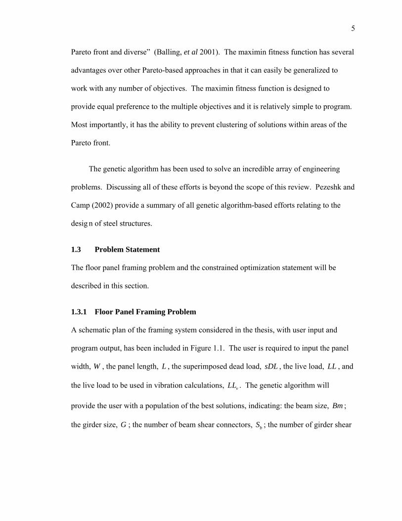
A schematic plan of the framing system considered in the thesis, with user input and
program output, has been included in Figure 1.1. The user is required to input the panel
width, W , the panel length, L , the superimposed dead load, sDL , the live load, LL , and
the live load to be used in vibration calculations, vLL . The genetic algorithm will
provide the user with a population of the best solutions, indicating: the beam size, Bm ;
the girder size, G ; the number of beam shear connectors, bS ; the number of girder shear
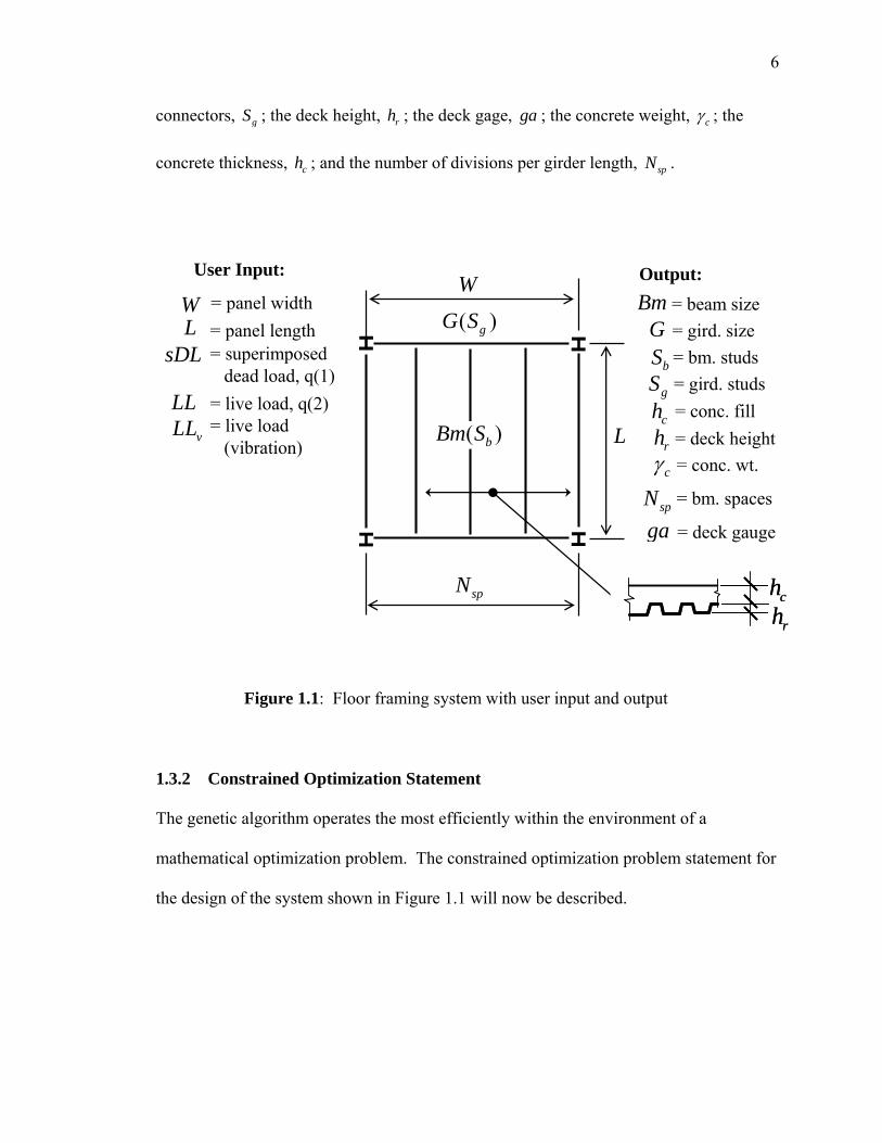
6
connectors, gS ; the deck height, rh ; the deck gage, ga ; the concrete weight, cγ ; the
concrete thickness, ch ; and the number of divisions per girder length, spN .
L
W
chrh
spN
Output:
( )gG S
( )bBm S
Bm
bSG
gS
chrh
User Input:
WL
sDL
= panel width= panel length= superimposed
dead load, q(1)LL = live load, q(2)
vLL = live load(vibration)
cγ
= beam size= gird. size= bm. studs= gird. studs= conc. fill= deck height= conc. wt.
spN
= bm. spaces
ga = deck gauge
1.3.2 Constrained Optimization Statement
The genetic algorithm operates the most efficiently within the environment of a
mathematical optimization problem. The constrained optimization problem statement for
the design of the system shown in Figure 1.1 will now be described.
Figure 1.1: Floor framing system with user input and output
chrhchrh
7
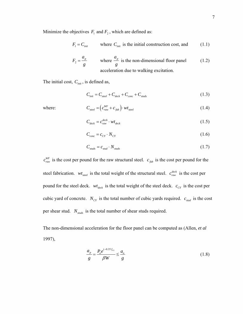
Minimize the objectives 1 2 and F F , which are defined as:
1 initF C= where initC is the initial construction cost, and (1.1)
2pa
Fg
= where pag
is the non-dimensional floor panel (1.2)
acceleration due to walking excitation.
The initial cost, initC , is defined as,
init steel deck conc studsC C C C C= + + + (1.3)
where: ( )WFsteel raw fab steelC c c wt= + ⋅ (1.4)
deckdeck raw deckC c wt= ⋅ (1.5)
conc CY CYC c N= ⋅ (1.6)
studs stud studsC c N= ⋅ (1.7)
WFrawc is the cost per pound for the raw structural steel. fabc is the cost per pound for the
steel fabrication. steelwt is the total weight of the structural steel. deckrawc is the cost per
pound for the steel deck. deckwt is the total weight of the steel deck. CYc is the cost per
cubic yard of concrete. CYN is the total number of cubic yards required. studc is the cost
per shear stud. studsN is the total number of shear studs required.
The non-dimensional acceleration for the floor panel can be computed as (Allen, et al
1997),
)( 0.35 nfp o oa P e a
g W gβ
−
= ≤ (1.8)
8
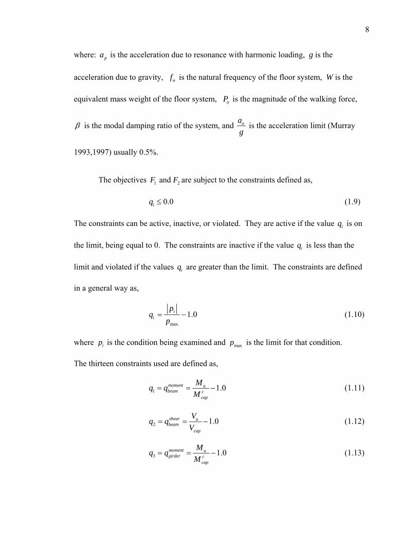
where: pa is the acceleration due to resonance with harmonic loading, g is the
acceleration due to gravity, nf is the natural frequency of the floor system, W is the
equivalent mass weight of the floor system, oP is the magnitude of the walking force,
β is the modal damping ratio of the system, and oag
is the acceleration limit (Murray
1993,1997) usually 0.5%.
The objectives 1 2 and F F are subject to the constraints defined as,
0.0iq ≤ (1.9)
The constraints can be active, inactive, or violated. They are active if the value iq is on
the limit, being equal to 0. The constraints are inactive if the value iq is less than the
limit and violated if the values iq are greater than the limit. The constraints are defined
in a general way as,
max
1.0ii
pq
p= − (1.10)
where ip is the condition being examined and maxp is the limit for that condition.
The thirteen constraints used are defined as,
1 1.0moment ubeam c
cap
Mq qM
= = − (1.11)
2 1.0shear ubeam
cap
Vq qV
= = − (1.12)
3 1.0moment ugirder c
cap
Mq qM
= = − (1.13)
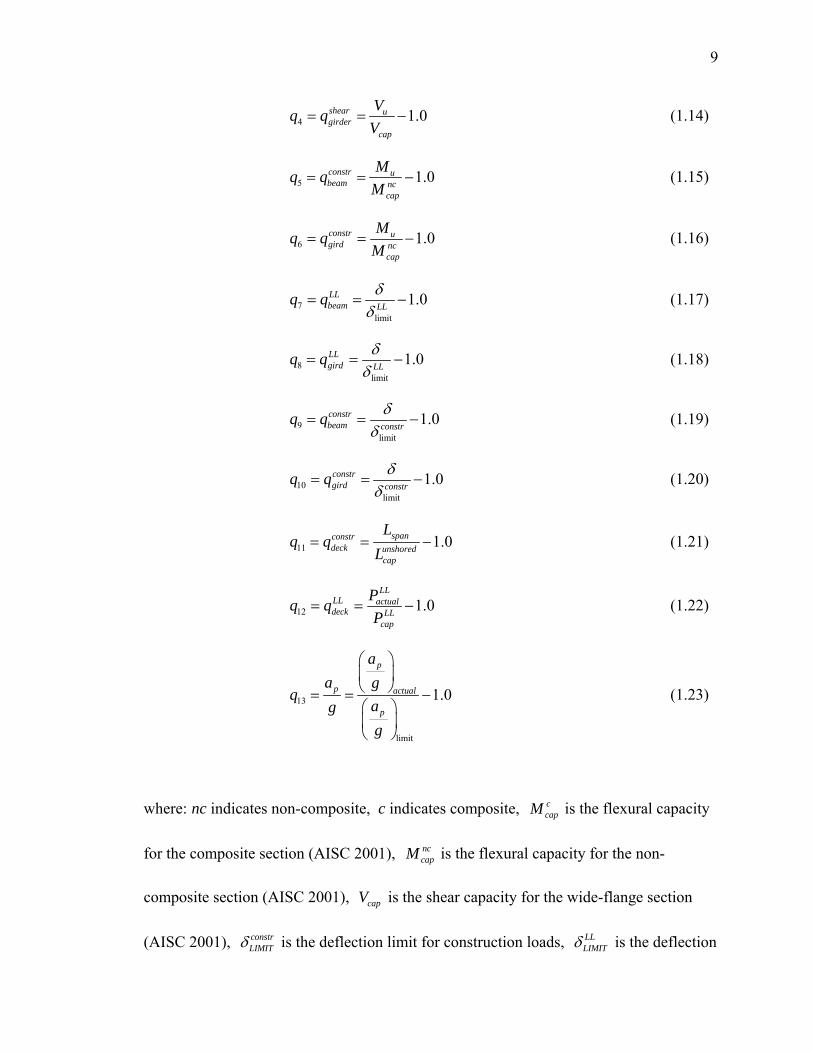
9
4 1.0shear ugirder
cap
Vq qV
= = − (1.14)
5 1.0constr ubeam nc
cap
Mq qM
= = − (1.15)
6 1.0constr ugird nc
cap
Mq qM
= = − (1.16)
7limit
1.0LLbeam LLq q δ
δ= = − (1.17)
8limit
1.0LLgird LLq q δ
δ= = − (1.18)
9limit
1.0constrbeam constrq q δ
δ= = − (1.19)
10limit
1.0constrgird constrq q δ
δ= = − (1.20)
11 1.0spanconstrdeck unshored
cap
Lq q
L= = − (1.21)
12 1.0LL
LL actualdeck LL
cap
Pq qP
= = − (1.22)
13
limit
1.0
p
p actual
p
aa g
qagg
⎛ ⎞⎜ ⎟⎝ ⎠= = −⎛ ⎞⎜ ⎟⎝ ⎠
(1.23)
where: nc indicates non-composite, c indicates composite, ccapM is the flexural capacity
for the composite section (AISC 2001), nccapM is the flexural capacity for the non-
composite section (AISC 2001), capV is the shear capacity for the wide-flange section
(AISC 2001), constrLIMITδ is the deflection limit for construction loads, LL
LIMITδ is the deflection

10
limit due to live load, unshoredcapL is the un-shored (3-span) limitation (Vulcraft 2001), and
LLcapp is the (3-span) superimposed loading capacity (Vulcraft 2001).
1.4 Overview of Contents
The size of the thesis warrants an overview of its contents. Chapter 2 presents general
details describing the operation of a genetic algorithm. Details specific to programming
the genetic algorithm in the MATLAB environment are included in Chapter 3. Necessary
design checks for strength and performance are summarized in Chapter 4. Eight design
examples are provided in Chapter 5 with analysis and observed trends. A summary,
conclusions, and recommendations for future work are presented in Chapter 6.

11
Chapter 2
Genetic Algorithm Fundamentals
A genetic algorithm (GA) is a search strategy that is modeled after the principles of
genetic evolution. The GA is especially useful for finding optimal or near-optimal
solutions to discrete variable optimization problems, like the floor framing design
presented with this thesis. The GA searches for the best possible combination of
individual system elements, but it does not do so in a conventional way.
Traditionally, an engineer uses a trial-and-error method to obtain a single solution
to the problem. This single solution may meet all specifications for strength and
performance, but it may not be the optimal solution based on minimizing total cost or
structure weight. With the increase in performance of the standard desktop computer, it
seems logical to write a program that will test and evaluate all possible combinations of
system elements. This method, referred to as an exhaustive search or complete
enumeration, is possible but can be quite lengthy, even with powerful computers.
For the floor framing problem presented, there are 256 beam and girder choices, 8
steel deck combinations, 8 concrete slab combinations, 32 beam and girder stud
configurations, and 4 panel layout choices. This leads to 17.2 billion unique solutions
which combine these parameters. An exhaustive search could be conducted to evaluate
each unique solution. A better method exists in the form of the genetic algorithm. The
GA does not evaluate each individual combination, but rather begins with a small
population of individual solutions with randomly chosen characteristics that improve as
they adapt to fitness parameters over the course of 30 to 40 generations. The GA proves

12
to be a fast and efficient way to solve the floor framing problem which involves a large
number of discrete design variables. The main steps involved in the operation of the GA
will be summarized in the following sections.
2.1 Encoding the Chromosome
The basic element of the genetic algorithm is the chromosome. The chromosome
contains the variable information for each individual solution to the problem.
The most common coding method is to represent each variable with a binary string of
digits with a specific length. As illustrated in Figure 3.1, the chromosome used in this
project includes a total of 34 binary digits grouped into 9 genes of varying length. The
string values for each gene are assigned to particular choices for the given characteristic,
so that they can be decoded later.
01101010 11000111 0 1 10 11 00 11001 00110
Girder (256 choices)
Beam (256 choices)
Conc. Type (LW or NW)
Deck Height (1.5 or 3.0 in.)
Conc. Height (4 choices)
Gauge (19,20,21,22)
Beam Studs (32 choices)
Girder Studs (32 choices)
Spacings (2,3,4,5)
Figure 2.1: Chromosomal representation (34 binary digits)

13
2.2 Creating the Initial Population
The genetic algorithm sequence begins with the creation of an initial population of
individuals. The size of the population is chosen by the program user. Random numbers
are used to generate the 1’s and 0’s that represent the genetic material of each individual.
With the chromosomes created, the binary string data of each solution must be converted
into useable problem data.
2.3 Evaluation of Fitness
The “fitness” of each individual solution is a quantitative measure of how well the
solution solves the original problem. The fitness is based on an objective function. For
this project, the objective function was defined in Section 1.3.2. Based on the fitness
values, individuals within the population are ranked from most-fit to least-fit.
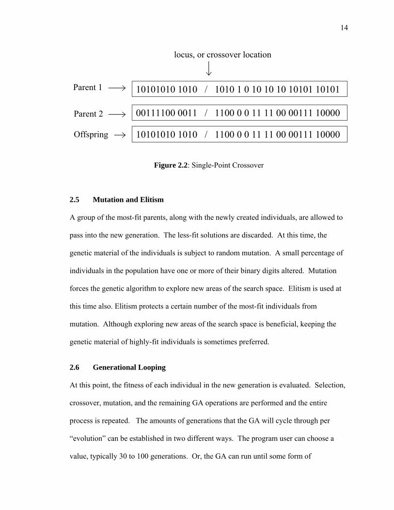
2.4 Crossover
Crossover is the process by which the genetic material of two “parents” will be combined
to create a new solution. Different selection methods exist for choosing the parents to be
involved in each crossover. The method used in this project is referred to as population
partitioning. This method gives more-fit individuals a higher probability of being
selected as a parent. The crossover process involves the combination of binary digits
from the two parent chromosomes. Different crossover methods can be used. The
simplest, and the one used in this project, is known as single-point crossover. A
crossover location, or locus, is selected randomly. The locus is shown in Figure 2.2. The
genetic material to the left of the locus of one parent is combined with the genetic
material to the right of the locus for the second parent. Each new individual is created in
this way.
14
Figure 2.2: Single-Point Crossover
2.5 Mutation and Elitism
A group of the most-fit parents, along with the newly created individuals, are allowed to
pass into the new generation. The less-fit solutions are discarded. At this time, the
genetic material of the individuals is subject to random mutation. A small percentage of
individuals in the population have one or more of their binary digits altered. Mutation
forces the genetic algorithm to explore new areas of the search space. Elitism is used at
this time also. Elitism protects a certain number of the most-fit individuals from
mutation. Although exploring new areas of the search space is beneficial, keeping the
genetic material of highly-fit individuals is sometimes preferred.
2.6 Generational Looping
At this point, the fitness of each individual in the new generation is evaluated. Selection,
crossover, mutation, and the remaining GA operations are performed and the entire
process is repeated. The amounts of generations that the GA will cycle through per
“evolution” can be established in two different ways. The program user can choose a
value, typically 30 to 100 generations. Or, the GA can run until some form of
10101010 1010 / 1010 1 0 10 10 10 10101 10101
00111100 0011 / 1100 0 0 11 11 00 00111 10000
10101010 1010 / 1100 0 0 11 11 00 00111 10000
Parent 1
Parent 2
Offspring
locus, or crossover location

15
“convergence” is reached. Convergence is based on the degree to which the best solution
is being improved upon in subsequent generations.

16
Chapter 3
Programming the GA in MATLAB
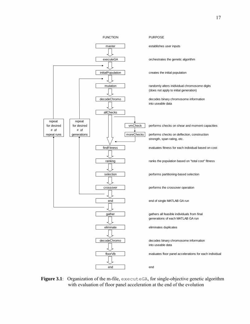
Three different versions of the genetic algorithm have been completed. The first version,
with its sequence shown in Figure 3.1, uses the single-objective fitness statement defined
in Section 1.3.2 and analyzes floor system accelerations due to walking excitation only at
the end of the evolution. The second version, with its sequence shown in Figure 3.2, uses
the same single-objective fitness statement but includes floor system accelerations due to
walking excitation within each generation as a penalty function. The third version, with
its sequence shown in Figure 3.3, is based on a multi-objective fitness statement. Floor
system accelerations due to walking excitation are included as the second objective.
Individual m-files will be summarized in the following sections.
3.1 FUNCTION: allChecks.m
The function allChecks.m is used to control two additional m-files that test for deflection,
strength, and performance violations for each individual in the population. The two
additional m-files are titled vmCheck.m and moreCheck.m.
vmCheck.m uses calculations to identify shear and moment capacity violations in
the composite beam and the composite girder for factored loading conditions.
17
FUNCTION PURPOSE
master establishes user inputs
executeGA orchestrates the genetic algorithm
initialPopulation creates the initial population
mutation randomly alters inidividual chromosome digits(does not apply to initial generation)
decodeChromo decodes binary chromosome information into useable data
allChecks
repeat repeat for desired for desired vmCheck performs checks on shear and moment capacities
# of # ofrepeat runs generations moreChecks performs checks on deflection, construction
strength, span rating, etc.
findFitness evaluates fitness for each individual based on cost
ranking ranks the population based on "total cost" fitness
selection performs partitioning-based selection
crossover performs the crossover operation
end end of single MATLAB GA run
gather gathers all feasible individuals from final generations of each MATLAB GA run
eliminate eliminates duplicates
decodeChromo decodes binary chromosome information into useable data
floorVib evaluates floor panel accelerations for each individual
end end Figure 3.1: Organization of the m-file, executeGA, for single-objective genetic algorithm with evaluation of floor panel acceleration at the end of the evolution

18
FUNCTION PURPOSE
master establishes user inputs
executeGA orchestrates the genetic algorithm
initialPopulation creates the initial population
mutation randomly alters individual chromosome digits(does not apply to initial generation)
decodeChromo decodes binary chromosome information into useable data
floorVib evaluates floor panel accelerations for each individual
allChecks
repeat vmCheck performs checks on shear and moment capacitiesfor desired
# of moreChecks performs checks on deflection, constructiongenerations strength, span rating, vibration, etc.
findFitness
ranking ranks the population based on maximin fitness
selection performs partitioning-based selection
crossover performs the crossover operation
end end
Figure 3.2: Organization of the m-file, executeGA, for single-objective genetic algorithm using floor panel acceleration as a penalty

19
FUNCTION PURPOSE
master establishes user inputs
executeGA orchestrates the genetic algorithm
initialPopulation creates the initial population
mutation randomly alters individual chromosome digits(does not apply to initial generation)
decodeChromo decodes binary chromosome information into useable data
allChecks
vmCheck performs checks on shear and moment capacities
moreChecks performs checks on deflection, constructionrepeat strength, span rating, etc.
for desired# of findFitness
generations
floorVib evaluates floor panel accelerations for each individual
maximin evaluates maximin fitness for each individual
ranking ranks the population based on maximin fitness
selection performs partitioning-based selection
crossover performs the crossover operation
end end
Figure 3.3: Organization of the m-file, executeGA, for multi-objective genetic algorithm using maximin fitness evaluation
20
moreCheck.m evaluates additional violations relating to deck, beam, and girder
strength, deflection, and performance. The first two checks in moreCheck.m are used to
verify beam and girder bending capacity during construction. The next two checks are
for deflection of the composite beam and deflection of the composite girder under live
load conditions. The following two checks are used to verify beam and girder deflections
during construction. Checks are next made for deck unshored clear span distance and
deck live load rating. An optional check, for floor panel acceleration, is used only within
the third version of the genetic algorithm presented with this thesis. This version uses a
single-objective fitness statement, but includes floor panel acceleration due to walking
excitation as a violation check.
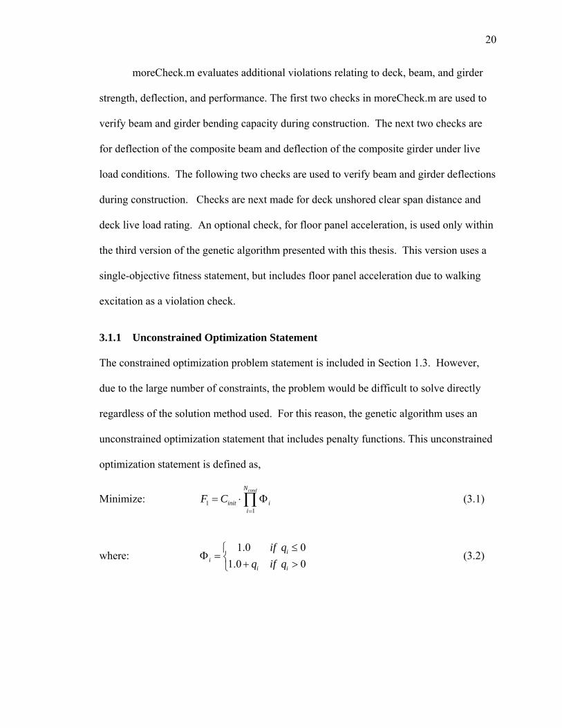
3.1.1 Unconstrained Optimization Statement
The constrained optimization problem statement is included in Section 1.3. However,
due to the large number of constraints, the problem would be difficult to solve directly
regardless of the solution method used. For this reason, the genetic algorithm uses an
unconstrained optimization statement that includes penalty functions. This unconstrained
optimization statement is defined as,
Minimize: 11
condN
init ii
F C=
= ⋅ Φ∏ (3.1)
where: 1.0 0
1.0 0i
ii i
if qq if q
≤⎧Φ = ⎨ + >⎩
(3.2)

21
initC and pag
are defined as equations (1.3) and (1.8), respectively, in Section 1.3.2. The
values iq are the constraints from the constrained optimization problem statement and are
defined in a general way by,
max
1.0ii
pq
p= − (3.3)
where ip is the condition being examined and maxp is the limit for that condition. The
individual constraints are defined by equations (1.11) to (1.23) in Section 1.3.2.
The difference between the constrained and unconstrained versions of the
optimization statement is subtle. In the constrained version, all constraints must always
be met for a solution to be considered. In the unconstrained version, the same conditions
iq are used, but they do not have to be met for a solution to be considered. If the
conditions are not met, the individual solution is simply modified with a penalty function.
Using this system, the genetic algorithm can start with poor solutions that violate the
conditions iq , and slowly improve them until they are within allowable limits.
22
4.1.3 Penalized Objective Function
The design checks made within the m-file allChecks.m are used as the basis for the
penalized objective function. The penalized objective function is used to decrease the
appeal of those individuals who do not meet any or all of the strength, deflection, and
performance conditions.
The objective function 1F , as shown in equation (3.1), is expressed as the product
of the total panel cost and penalties, where condN is the number of violation conditions
for the problem and iΦ is the penalty corresponding to the ith condition.
If an individual in the population exceeds one or more of the violation conditions,
then a penalty is applied to the individual’s fitness value. A multiple linear segment
penalty function is used, which relates the value of an individual penalty to the degree in
which the violation condition has been exceeded. As illustrated in equation (3.2) of the
previous section, this means that as long as the selected parameter is less than the given
limit, the penalty iΦ is 1.0, having no effect on the objective function. But when the
parameter limit is exceeded, the penalty grows in a linear manner and is equal to the
given value of the parameter divided by the limit.
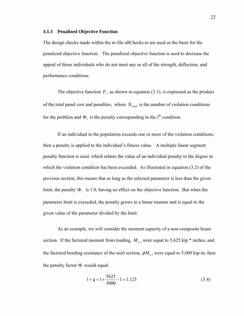
As an example, we will consider the moment capacity of a non-composite beam
section. If the factored moment from loading, uM , were equal to 5,625 kip * inches, and
the factored bending resistance of the steel section, nMφ , were equal to 5,000 kip-in, then
the penalty factor Φ would equal:
56251 1 1 1.1255000
q+ = + − =
(3.4)
23
So, the penalty for this violation, moment capacity of the non-composite beam section,
would be equal to 1.125. The value of the objective function for this individual would
be increased by 12.5%, making the individual less desirable to the genetic algorithm as a
solution. If an individual violates more than one penalty, the product of the individual
penalty functions is applied to the individual’s fitness.
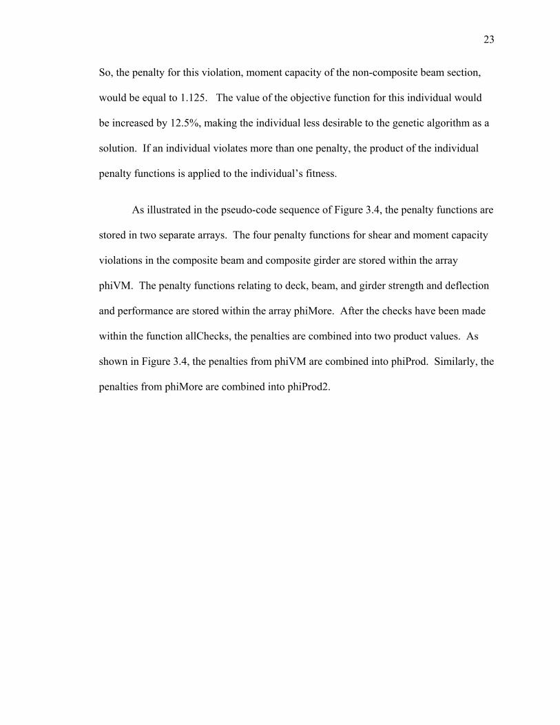
As illustrated in the pseudo-code sequence of Figure 3.4, the penalty functions are
stored in two separate arrays. The four penalty functions for shear and moment capacity
violations in the composite beam and composite girder are stored within the array
phiVM. The penalty functions relating to deck, beam, and girder strength and deflection
and performance are stored within the array phiMore. After the checks have been made
within the function allChecks, the penalties are combined into two product values. As
shown in Figure 3.4, the penalties from phiVM are combined into phiProd. Similarly, the
penalties from phiMore are combined into phiProd2.

24
____________________________________________________________________
WITHIN allChecks:
[phiVM] = vmCheck(sysIn,allProps,popSize) ;
phiVM = [phiVb;phiMb;phiVg;phiMg] ;
[phiMore] = moreCheck(sysIn,allProps,popSize) ;
phiMore = [unshoredDeck;beamAlone;girdAlone;deflDeck;deflBeamConstr;…
deflGirdConstr;deflBeam;deflGird;ratingDeck] ;
for indiv = 1:popSize
phiProd(indiv) = phiVM(1,indiv) * phiVM(2,indiv) * phiVM(3,indiv)* phiVM(4,indiv) ;
end
for indiv = 1:popSize
phiProd2(indiv) = phiMore(1,indiv) * phiMore(2,indiv) * phiMore(3,indiv) ...
* phiMore(4,indiv) * phiMore(5,indiv) * phiMore(6,indiv) * phiMore(7,indiv) ...
* phiMore(8,indiv) * phiMore(9,indiv) ;
end
________________________________________________________________________
Figure 3.4: Pseudo-code detailing arrays phiProd and phiProd2, which contain penalty values from strength and deflection checks
3.2 FUNCTION: crossover.m
The function crossover.m is used to combine the genetic material from two selected
parents in order to form each new individual for the subsequent generation. This
function uses the array mate_indiv, which was created during the selection process.
mate_indiv contains the two parent identifiers for each new individual, as well as the
locus for each crossover . The locus, or crossover location, is the point where each of the
two parent chromosomes will be split. The genetic material of parent 1 which lies to the
left of the locus will be combined with the genetic material of parent two which lies to
the right of the locus, in order to form the new individual. This form of crossover is

25
termed single-point crossover. It is the most basic crossover method, but is very effective
in combining traits of two parents into a single offspring. For this reason, it is commonly
used within the GA community.
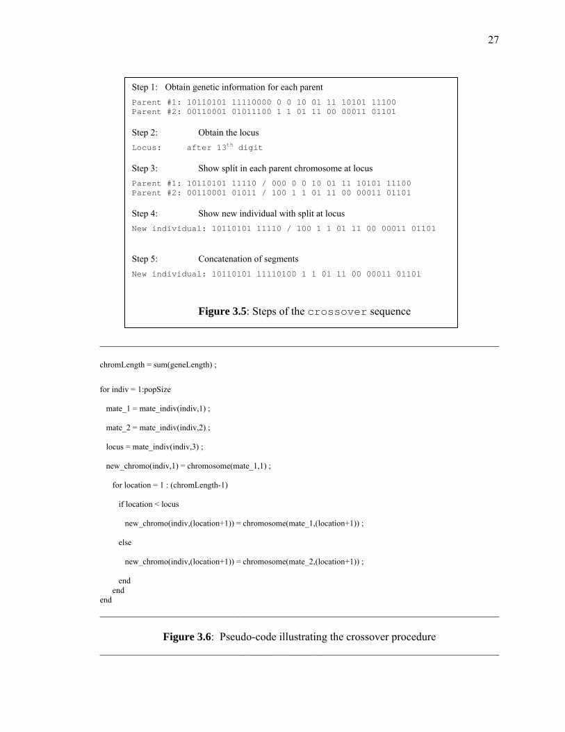
The steps required to execute the crossover operation in MATLAB will be
discussed. A sample crossover sequence is shown in Figure 3.5 in order to illustrate the
steps of the process. The pseudo-code for this operation is included in Figure 3.6. The
length of the chromosome is first computed by summing the number of digits in each of
the nine genes. For the versions of the genetic algorithm being used in this project, this
length is always equal to 34 digits. Beginning with the first new individual to be created,
identifiers for each parent are obtained, as is the locus, or crossover point. The first digit
for the new individual is always obtained from parent 1. It is placed in the first spot in the
first row of the array new_chromo.
Additional digits are taken from parent 1, and copied into new_chromo, until the
locus has been reached. To the right of the locus, information from parent 2 is used to fill
in the remaining digits of the first row of new_chromo. Left and right segments of the
new individual are concatenated, or combined. This procedure is repeated a number of
times equal to the population size.
26
3.3 FUNCTION: decodeChromo.m
The function decodeChromo.m is used to decode the binary information stored within the
chromosome into useable problem data. The groups of binary digits are first converted
into integer values which are used to identify certain characteristics. Next, the integer
identifiers are used to retrieve useable information for the specified characteristic. Lastly,
a single array titled allProps is created, which contains all the necessary problem data for
each individual in the current generation.
As illustrated in the section of pseudo-code presented as Figure 3.7, the first step
is to decode individual genes within the chromosome into integer values. The genes are
groups of digits, or alleles, within the chromosome. For the programs presented with this
thesis, there are always nine genes in the chromosome. They represent the girder section,
the beam section, the concrete type, the deck height, the concrete thickness, the deck
gage, the number of divisions per girder length (bays), the number of shear studs per half
beam, and the number of shear studs per half girder. Once converted, the integer
identifiers are stored in the array unknowns, which is of size (popSize x numUNKNO),
where numUNKNO is the number of genes per individual. Again, numUNKNO will
always be equal to nine.
27
________________________________________________________________________ chromLength = sum(geneLength) ;
for indiv = 1:popSize
mate_1 = mate_indiv(indiv,1) ;
mate_2 = mate_indiv(indiv,2) ;
locus = mate_indiv(indiv,3) ;
new_chromo(indiv,1) = chromosome(mate_1,1) ;
for location = 1 : (chromLength-1)
if location < locus
new_chromo(indiv,(location+1)) = chromosome(mate_1,(location+1)) ;
else
new_chromo(indiv,(location+1)) = chromosome(mate_2,(location+1)) ;
end end end ________________________________________________________________________
Figure 3.6: Pseudo-code illustrating the crossover procedure ________________________________________________________________________
Step 1: Obtain genetic information for each parent
Parent #1: 10110101 11110000 0 0 10 01 11 10101 11100 Parent #2: 00110001 01011100 1 1 01 11 00 00011 01101 Step 2: Obtain the locus
Locus: after 13th digit Step 3: Show split in each parent chromosome at locus
Parent #1: 10110101 11110 / 000 0 0 10 01 11 10101 11100 Parent #2: 00110001 01011 / 100 1 1 01 11 00 00011 01101 Step 4: Show new individual with split at locus
New individual: 10110101 11110 / 100 1 1 01 11 00 00011 01101 Step 5: Concatenation of segments
New individual: 10110101 11110100 1 1 01 11 00 00011 01101
Figure 3.5: Steps of the crossover sequence

28
for i = 1:popSize
bit = 1 ;
for j = 1:numUNKNO
unknowns(i,j) = 0 ;
for allele = 1:geneLength(j)
if chromosome(i,bit) == 1
unknowns(i,j) = unknowns(i,j) + 2^(allele-1) ;
end
if bit <= chromLength
bit = bit + 1 ;
else
break
end
end
end
end
________________________________________________________________________
Figure 3.7: Pseudo-code used for decoding chromosome information into integer values
___________________________________________________________
for i = 1:popSize
for j = 1:numUNKNO
unknowns(i,j) = unknowns(i,j) + 1 ;
end
end
___________________________________________________________
Figure 3.8: Pseudo-code used for adding 1 to each integer value for consistent labeling
29
It should be noted that individual binary digits within the chromosome are ordered
with the most significant digit being to the right. Thus, the binary number 011 is
represented by [ 0 * 20 + 1 * 21 + 1 * 22 ] and would be equal to 6. If converted in the
conventional manner, the number would be calculated according to [ 0 * 22 + 1 * 21 +
1 * 20 ] and would be equal to 3.
An example of the encoding/decoding process in included in the following
section. This same example will be revisited as additional decoding information is
presented. The chromosome given as,
chromosome = 01101100 10101011 0 1 01 11 00 11111 10101
will be used in the example. After the genes of the chromosome are converted to integer
values, the corresponding line within the array unknowns would be as follows,
unknowns = 54 213 0 1 2 3 0 31 21.
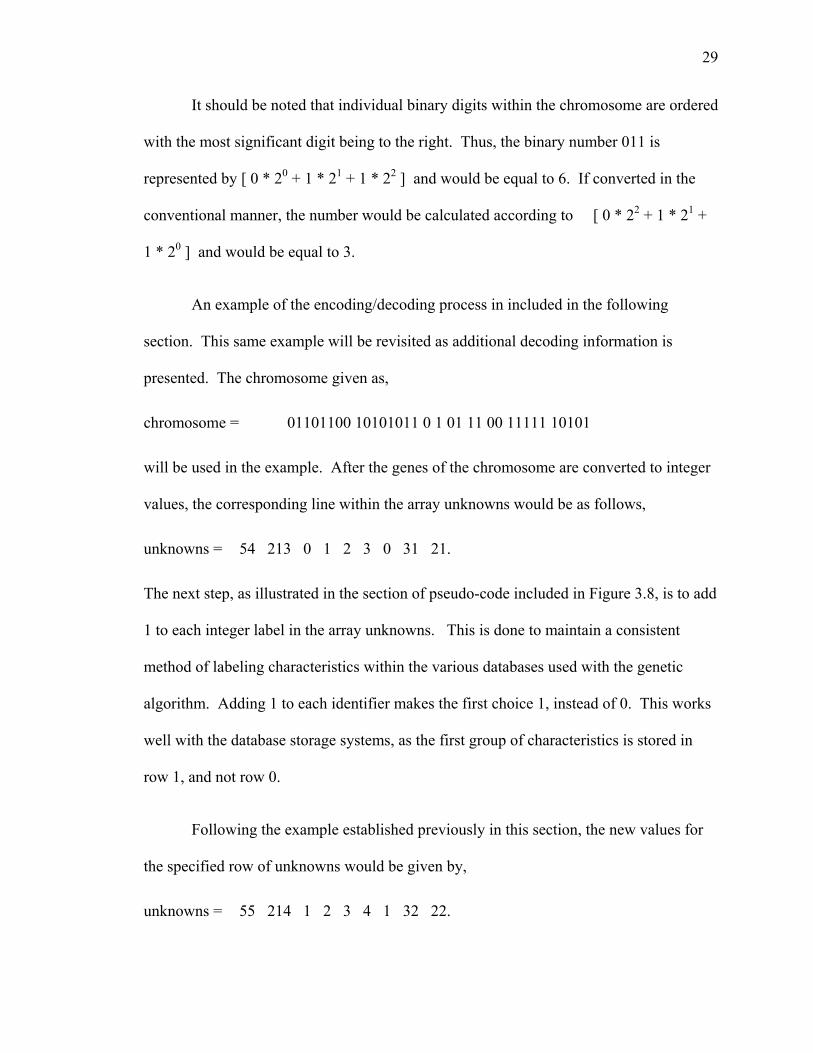
The next step, as illustrated in the section of pseudo-code included in Figure 3.8, is to add
1 to each integer label in the array unknowns. This is done to maintain a consistent
method of labeling characteristics within the various databases used with the genetic
algorithm. Adding 1 to each identifier makes the first choice 1, instead of 0. This works
well with the database storage systems, as the first group of characteristics is stored in
row 1, and not row 0.
Following the example established previously in this section, the new values for
the specified row of unknowns would be given by,
unknowns = 55 214 1 2 3 4 1 32 22.
30
The next step within decodeChromo involves using the integer identifiers to retrieve
appropriate data for each characteristic of each individual. The process for retrieving
data for all nine characteristics is discussed next.
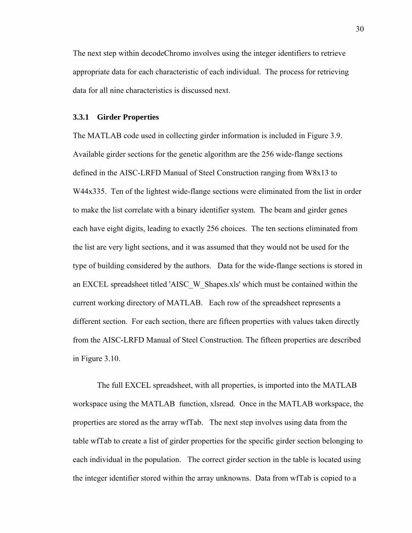
3.3.1 Girder Properties
The MATLAB code used in collecting girder information is included in Figure 3.9.
Available girder sections for the genetic algorithm are the 256 wide-flange sections
defined in the AISC-LRFD Manual of Steel Construction ranging from W8x13 to
W44x335. Ten of the lightest wide-flange sections were eliminated from the list in order
to make the list correlate with a binary identifier system. The beam and girder genes
each have eight digits, leading to exactly 256 choices. The ten sections eliminated from
the list are very light sections, and it was assumed that they would not be used for the
type of building considered by the authors. Data for the wide-flange sections is stored in
an EXCEL spreadsheet titled 'AISC_W_Shapes.xls' which must be contained within the
current working directory of MATLAB. Each row of the spreadsheet represents a
different section. For each section, there are fifteen properties with values taken directly
from the AISC-LRFD Manual of Steel Construction. The fifteen properties are described
in Figure 3.10.
The full EXCEL spreadsheet, with all properties, is imported into the MATLAB
workspace using the MATLAB function, xlsread. Once in the MATLAB workspace, the
properties are stored as the array wfTab. The next step involves using data from the
table wfTab to create a list of girder properties for the specific girder section belonging to
each individual in the population. The correct girder section in the table is located using
the integer identifier stored within the array unknowns. Data from wfTab is copied to a

31
new array, wfGird. The array wfGird is of size ( popSize x 15 ) and contains only the
specific section properties for the girder of each individual in the population. Following
the example established within this section, the corresponding row of the array unknowns
is given as,
unknowns = 55 214 1 2 3 4 1 32 22.
Column one corresponds to the girder, and is shown as 55. This means that the
individual who is represented by this data is using girder number 55 in the list of
available sections. By looking in the EXCEL spreadsheet, it can be seen that section
number 55 is for a W12x230 section. (This is actually a column section, but this fact
presents no difficulties for this example. It should be noted that column sections were
included in the list of available sections as an experiment to see if they would prove
useful in minimizing floor panel acceleration values.) The information corresponding to
this row of the array wfTab is copied into the new array, wfGird. The row of values
representing the girder of this individual in the array wfGird is given as,
wfGird = 12 230 67.7 15.1 1.29 12.9 2.07 2420 321 5.97 386 742 115 3.31 177
A listing of descriptions for these values can be seen on the previously mentioned table
shown as Figure 3.10.
_______________________________________________________________________________

32
wfTab = xlsread('AISC_W_Shapes.xls') ;
for indiv = 1:popSize
wfGird(indiv,:) = wfTab(unknowns(indiv,1),:) ;
end
________________________________________________________________________
Figure 3.9: MATLAB code used for importing girder properties
_______________________________________________________________________
1....Nominal section depth, in inches 2....Weight per foot, in pounds 3....Gross Area, Ag, in inches ^ 2 4....Depth, d, in inches 5....Web Thickness,tw, in inches 6....Flange Width, bf, in inches 7....Flange Thickness, tf, in inches 8....I for X-X Axis, in inches ^ 4 9....S for X-X Axis, in inches ^ 3 10...r for X-X Axis, in inches 11...Z for X-X Axis, in inches ^ 3 12...I for Y-Y Axis, in inches ^ 4 13...S for Y-Y Axis, in inches ^ 3 14...r for Y-Y Axis, in inches 15...Z for Y-Y Axis, in inches ^ 3
_______________________________________________________________________
Figure 3.10: Description of the fifteen girder properties
3.3.2 Beam Properties
Beam properties are collected and stored in the same manner as the girder properties.
The same group of 256 wide-flange sections is available to the genetic algorithm as beam
sections. The one change is that section properties specific to the beam of each individual
are contained within the array wfBeam.
For use later in this section, the beam identifier for the previous example problem
will be decoded. The corresponding row of the array unknowns is given as:

33
unknowns = 55 214 1 2 3 4 1 32 22.
Column two in the array corresponds to the beam, and is shown as 214. This means that
the individual who is represented by this data is using beam number 214 in the list of
available sections. By looking in the EXCEL spreadsheet, it can be seen that section
number 214 is for a W36x182.
3.3.3 Steel Deck and Concrete Slab Properties
The next group of properties for each individual in the population is related to four of the
nine genes in the chromosome. These four genes are the concrete type gene, the deck
height gene, the concrete thickness gene, and the steel deck gage gene.
To begin the process, the concrete type identifier and the steel deck gage identifier
in the array unknowns are examined. There are two choices for each, leading to a total of
four different combinations of concrete type and deck gage. These four combinations are
light-weight concrete with a 1.5-inch deck height (LW 1.5), normal-weight concrete with
a 1.5-inch deck height (NW 1.5), light-weight concrete with a 3.0-inch deck height (LW
3.0), and normal-weight concrete with a 3.0-inch deck height (NW 3.0). Data for each of
the four combinations from the Vulcraft Steel Roof and Floor Deck manual (Vulcraft
2001) are stored in four separate EXCEL spreadsheets titled ‘LW_1_5.xls,’
‘NW_1_5.xls,’ ‘LW_3_0.xls,’ and ‘NW_3_0.xls.’ It should be noted that each of these
four EXCEL files must be contained within the current MATLAB working directory.
For each of the four combinations of concrete type and deck height, there are
sixteen additional combinations of deck gage and concrete height. For each combination
of concrete type and deck height, there are four choices of deck gage, which are 22, 21,
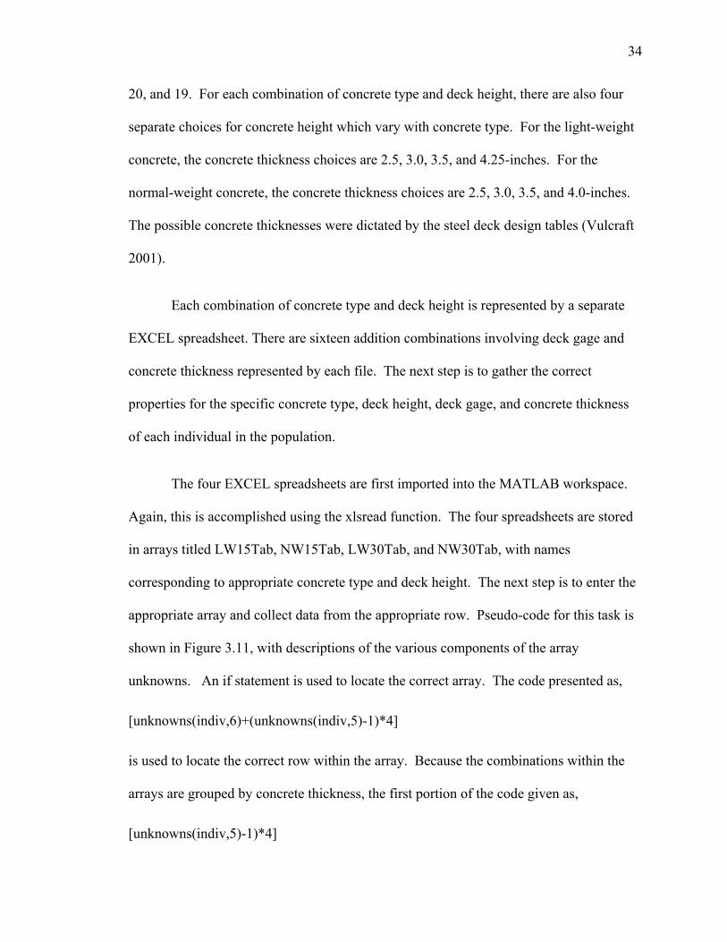
34
20, and 19. For each combination of concrete type and deck height, there are also four
separate choices for concrete height which vary with concrete type. For the light-weight
concrete, the concrete thickness choices are 2.5, 3.0, 3.5, and 4.25-inches. For the
normal-weight concrete, the concrete thickness choices are 2.5, 3.0, 3.5, and 4.0-inches.
The possible concrete thicknesses were dictated by the steel deck design tables (Vulcraft
2001).
Each combination of concrete type and deck height is represented by a separate
EXCEL spreadsheet. There are sixteen addition combinations involving deck gage and
concrete thickness represented by each file. The next step is to gather the correct
properties for the specific concrete type, deck height, deck gage, and concrete thickness
of each individual in the population.
The four EXCEL spreadsheets are first imported into the MATLAB workspace.
Again, this is accomplished using the xlsread function. The four spreadsheets are stored
in arrays titled LW15Tab, NW15Tab, LW30Tab, and NW30Tab, with names
corresponding to appropriate concrete type and deck height. The next step is to enter the
appropriate array and collect data from the appropriate row. Pseudo-code for this task is
shown in Figure 3.11, with descriptions of the various components of the array
unknowns. An if statement is used to locate the correct array. The code presented as,
[unknowns(indiv,6)+(unknowns(indiv,5)-1)*4]
is used to locate the correct row within the array. Because the combinations within the
arrays are grouped by concrete thickness, the first portion of the code given as,
[unknowns(indiv,5)-1)*4]
35
allows movement to the correct grouping of concrete thickness, while the second part,
[unknowns(indiv,6)]
allows movement within the grouping of concrete thicknesses to the correct deck gage.
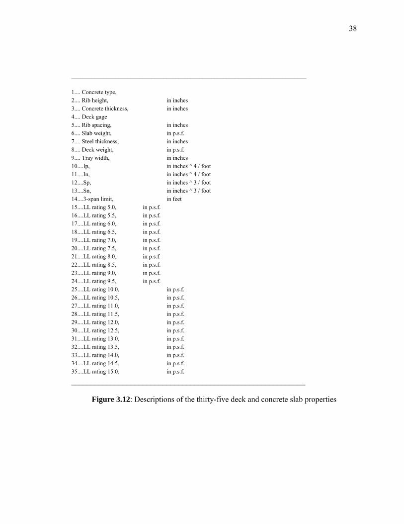
The arrays contain 35 properties for each combination of concrete type, deck
height, deck gage, and concrete height. The properties included are defined in Figure
3.12. The properties relating to the choice of concrete type, deck height, deck gage, and
concrete height for each individual are stored within the array stDeck.
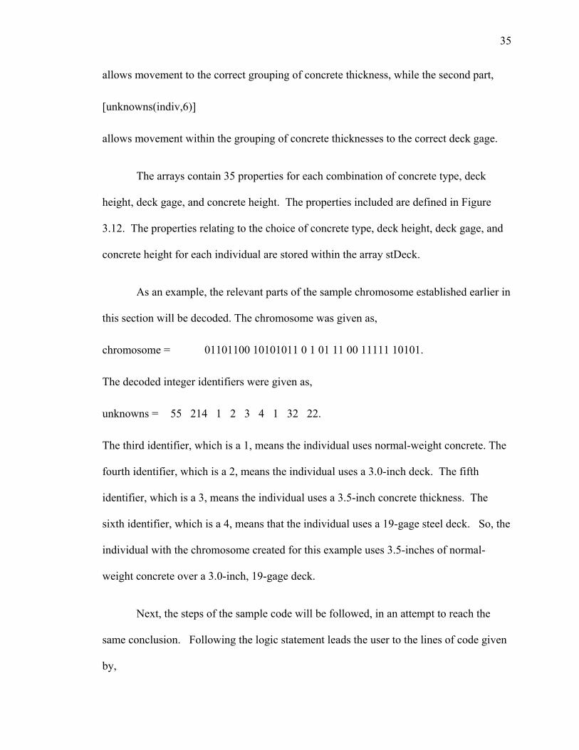
As an example, the relevant parts of the sample chromosome established earlier in
this section will be decoded. The chromosome was given as,
chromosome = 01101100 10101011 0 1 01 11 00 11111 10101.
The decoded integer identifiers were given as,
unknowns = 55 214 1 2 3 4 1 32 22.
The third identifier, which is a 1, means the individual uses normal-weight concrete. The
fourth identifier, which is a 2, means the individual uses a 3.0-inch deck. The fifth
identifier, which is a 3, means the individual uses a 3.5-inch concrete thickness. The
sixth identifier, which is a 4, means that the individual uses a 19-gage steel deck. So, the
individual with the chromosome created for this example uses 3.5-inches of normal-
weight concrete over a 3.0-inch, 19-gage deck.
Next, the steps of the sample code will be followed, in an attempt to reach the
same conclusion. Following the logic statement leads the user to the lines of code given
by,

36
elseif unknowns(indiv,3) == 1 & unknowns(indiv,4) == 2 ;
stDeck(indiv,:)=NW30Tab((unknowns((indiv,5)-1)*4)... +unknowns(indiv,6)),:);.
The location of the desired row is given by the code,
(unknowns((indiv,5)-1)*4)+unknowns(indiv,6)).
This location equals [(3-1)*4] + 4 = 8 + 4 = 12. So, the user should look at the twelfth
row in the array titled NW30Tab. This row begins with the numbers:
145 3 3.5 19
The first number represents the density of normal-weight concrete (in p.c.f.). The second
number indicates the 3.0-inch deck height. The third indicates a 3.5-inch concrete
thickness. And, the fourth number indicates a 19-gage deck. So, the function has led to
the correct row in the correct array.
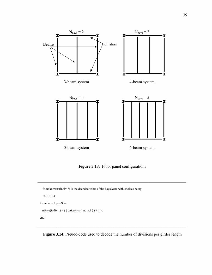
3.3.4 Number of Divisions per Girder Length
The baysGene contains information detailing how many divisions will be created by the
beams that frame into the girder. Choices for this variable are two, three, four, and five
divisions with configurations that are illustrated in Figure 3.13.
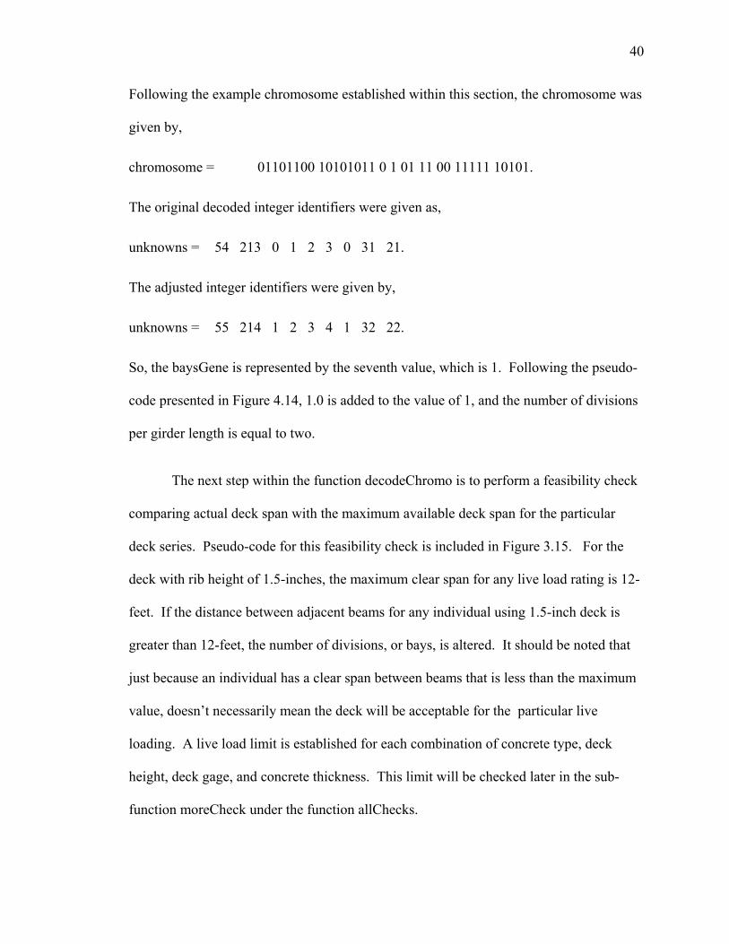
The pseudo-code used to decode the number of divisions per girder length is
included as Figure 3.14. It should be noted that 1.0 was added to the decoded values
earlier within this function to maintain a consistent labeling system. This step left the
four choices, actually integer identifiers, as 1,2,3,and 4. In this section of code, 1.0 is
again added to the decoded values to convert from integer identifier to actual number of
divisions per girder length. The four new choices are 2,3,4,and 5.

37
________________________________________________________________________
% unknowns(indiv,3) is the concrete type identifier
% unknowns(indiv,4) is the deck height identifier
% unknowns(indiv,5) is the concrete thickness identifier
% unknowns(indiv,6) is the deck gage identifier
for indiv = 1:popSize
if unknowns(indiv,3) == 1 & unknowns(indiv,4) == 1 ;
stDeck(indiv,:)=NW15Tab((unknowns((indiv,5)-1)*4)+unknowns(indiv,6)),:) ;
elseif unknowns(indiv,3) == 1 & unknowns(indiv,4) == 2 ;
stDeck(indiv,:)=NW30Tab((unknowns((indiv,5)-1)*4)+unknowns(indiv,6)),:) ;
elseif unknowns(indiv,3) == 2 & unknowns(indiv,4) == 1 ;
stDeck(indiv,:)=LW15Tab((unknowns((indiv,5)-1)*4)+unknowns(indiv,6)),:) ;
else unknowns(indiv,3) == 2 & unknowns(indiv,4) == 2 ;
stDeck(indiv,:)=LW30Tab((unknowns((indiv,5)-1)*4)+unknowns(indiv,6)),:) ;
end
end
________________________________________________________________________
Figure 3.11: Pseudo-code used for importing deck and concrete slab properties
38
_______________________________________________________________________________ 1.... Concrete type, 2.... Rib height, in inches 3.... Concrete thickness, in inches 4.... Deck gage 5.... Rib spacing, in inches 6.... Slab weight, in p.s.f. 7.... Steel thickness, in inches 8.... Deck weight, in p.s.f. 9.... Tray width, in inches 10....Ip, in inches ^ 4 / foot 11....In, in inches ^ 4 / foot 12....Sp, in inches ^ 3 / foot 13....Sn, in inches ^ 3 / foot 14....3-span limit, in feet 15....LL rating 5.0, in p.s.f. 16....LL rating 5.5, in p.s.f. 17....LL rating 6.0, in p.s.f. 18....LL rating 6.5, in p.s.f. 19....LL rating 7.0, in p.s.f. 20....LL rating 7.5, in p.s.f. 21....LL rating 8.0, in p.s.f. 22....LL rating 8.5, in p.s.f. 23....LL rating 9.0, in p.s.f. 24....LL rating 9.5, in p.s.f. 25....LL rating 10.0, in p.s.f. 26....LL rating 10.5, in p.s.f. 27....LL rating 11.0, in p.s.f. 28....LL rating 11.5, in p.s.f. 29....LL rating 12.0, in p.s.f. 30....LL rating 12.5, in p.s.f. 31....LL rating 13.0, in p.s.f. 32....LL rating 13.5, in p.s.f. 33....LL rating 14.0, in p.s.f. 34....LL rating 14.5, in p.s.f. 35....LL rating 15.0, in p.s.f.
___________________________________________________________
Figure 3.12: Descriptions of the thirty-five deck and concrete slab properties
39
______________________________________________________________________________
% unknowns(indiv,7) is the decoded value of the baysGene with choices being
% 1,2,3,4
for indiv = 1:popSize
nBays(indiv,1) = ( ( unknowns( indiv,7 ) ) + 1 ) ;
end
______________________________________________________________________________
Figure 3.14: Pseudo-code used to decode the number of divisions per girder length
Nbays = 2 Nbays = 3
Figure 3.13: Floor panel configurations
3-beam system 4-beam system
5-beam system 6-beam system
GirdersBeams
Nbays = 4 Nbays = 5
40
Following the example chromosome established within this section, the chromosome was
given by,
chromosome = 01101100 10101011 0 1 01 11 00 11111 10101.
The original decoded integer identifiers were given as,
unknowns = 54 213 0 1 2 3 0 31 21.
The adjusted integer identifiers were given by,
unknowns = 55 214 1 2 3 4 1 32 22.
So, the baysGene is represented by the seventh value, which is 1. Following the pseudo-
code presented in Figure 4.14, 1.0 is added to the value of 1, and the number of divisions
per girder length is equal to two.
The next step within the function decodeChromo is to perform a feasibility check
comparing actual deck span with the maximum available deck span for the particular
deck series. Pseudo-code for this feasibility check is included in Figure 3.15. For the
deck with rib height of 1.5-inches, the maximum clear span for any live load rating is 12-
feet. If the distance between adjacent beams for any individual using 1.5-inch deck is
greater than 12-feet, the number of divisions, or bays, is altered. It should be noted that
just because an individual has a clear span between beams that is less than the maximum
value, doesn’t necessarily mean the deck will be acceptable for the particular live
loading. A live load limit is established for each combination of concrete type, deck
height, deck gage, and concrete thickness. This limit will be checked later in the sub-
function moreCheck under the function allChecks.
41
Similarly, for the deck with rib height of 3.0-inches, the maximum clear span for
any live load rating is 15-feet. If the distance between adjacent beams for any individual
using 3.0-inch deck is greater than 15-feet, the number of divisions, or bays, is altered.
Again, it should be noted by the reader that just because an individual has a clear span
between beams that is less than the maximum value, doesn’t necessarily mean the deck
will be acceptable for the particular live loading. A superimposed live load limit is
established for each combination of concrete type, deck height, deck gage, and concrete
thickness. As before, this limit will be checked later in the sub-function moreCheck
described in Section 3.12.
The pseudo-code in Figure 3.15 uses the gene_repair sub-function. This sub-
function is used to fix the original chromosome after changes have been made to the
individual’s characteristics. More information on gene_repair can be found in Section
3.5.3.
For the example individual that has been examined throughout this section, it has
been determined that the individual will use two divisions per girder length and a 3.0-
inch deck. The maximum possible span for the 3.0-inch deck is 15-feet, so the individual
presented in this example will be acceptable as long as the girder length is no greater than
30-feet. For girder lengths greater than 30-feet, the number of divisions per girder length
would need to be increased and the associated gene repair procedure would be utilized.
Again, the reader should note that this is just a preliminary feasibility check, and that the
individual presented in this example will later need to be checked to see if the given live
load is acceptable for the indicated span.
3.3.5 Number of Shear Studs per Half Beam
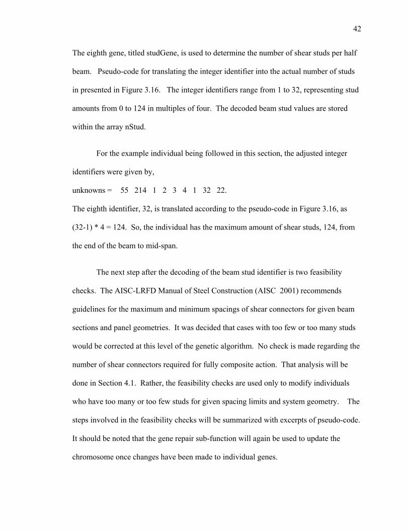
42
The eighth gene, titled studGene, is used to determine the number of shear studs per half
beam. Pseudo-code for translating the integer identifier into the actual number of studs
in presented in Figure 3.16. The integer identifiers range from 1 to 32, representing stud
amounts from 0 to 124 in multiples of four. The decoded beam stud values are stored
within the array nStud.
For the example individual being followed in this section, the adjusted integer
identifiers were given by,
unknowns = 55 214 1 2 3 4 1 32 22.
The eighth identifier, 32, is translated according to the pseudo-code in Figure 3.16, as
(32-1) * 4 = 124. So, the individual has the maximum amount of shear studs, 124, from
the end of the beam to mid-span.
The next step after the decoding of the beam stud identifier is two feasibility
checks. The AISC-LRFD Manual of Steel Construction (AISC 2001) recommends
guidelines for the maximum and minimum spacings of shear connectors for given beam
sections and panel geometries. It was decided that cases with too few or too many studs
would be corrected at this level of the genetic algorithm. No check is made regarding the
number of shear connectors required for fully composite action. That analysis will be
done in Section 4.1. Rather, the feasibility checks are used only to modify individuals
who have too many or too few studs for given spacing limits and system geometry. The
steps involved in the feasibility checks will be summarized with excerpts of pseudo-code.
It should be noted that the gene repair sub-function will again be used to update the
chromosome once changes have been made to individual genes.
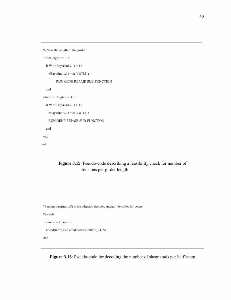
43
_______________________________________________________________________
% W is the length of the girder
if ribHeight == 1.5
if W / nBays(indiv,1) > 12
nBays(indiv,1) = ceil(W/12) ;
RUN GENE REPAIR SUB-FUNCTION
end
elseif ribHeight == 3.0
if W / nBays(indiv,1) > 15
nBays(indiv,1) = ceil(W/15) ;
RUN GENE REPAIR SUB-FUNCTION
end
end
end
________________________________________________________________________
Figure 3.15: Pseudo-code describing a feasibility check for number of divisions per girder length
________________________________________________________________________
% unknowns(indiv,8) is the adjusted decoded integer identifier for beam
% studs
for indiv = 1:popSize
nStud(indiv,1) = ((unknowns(indiv,8))-1)*4 ;
end
________________________________________________________________________
Figure 3.16: Pseudo-code for decoding the number of shear studs per half beam

44
Maximum number of shear connectors per half beam
All shear connector spacing guidelines have been taken from the Manual of Steel
Construction, Section I 5.6 (AISC 2001). Guidelines for shear connector spacing have
been taken from the appropriate areas of the manual for the case where steel deck ribs run
perpendicular to the beams. Pseudo-code detailing the first beam stud feasibility check
is presented as Figure 3.17.
The maximum number of shear connectors for the beam section due to spacing
constraints will be determined first. The first step is to figure out how many shear
connectors will fit within each valley in the transverse direction. The recommended
(AISC 2001) minimum center to center shear connector spacing of 4 cd⋅ , where cd is the
shear connector diameter (inches). For the typical shear connector with 0.75-inch
diameter, this spacing would be 3.0-inches. The variable for the number of shear
connectors that will fit side by side in the transverse direction is partners. The reader
should refer to the code in Figure 3.17 for details of the calculation. It should be noted
that for the calculation of the maximum number of shear connectors per half beam,
multiple studs in the direction transverse to the beam length are used if they meet spacing
requirements.
The example individual established earlier will be examined in regards to this
feasibility check. The beam for the example individual was a W36x182. The flange
width for this beam section is 12.075-inches, and was obtained from the array allProps.
According to the calculation for partners given by,
partners = floor ( ( flangeWidth - studDia ) / … ( 4 * studDia ) ) + 1

45
the number of shear connectors that would be allowed in the transverse direction would
be equal to [ ( (12.075-0.75) / 3 ) + 1.0 ] rounded down to the next integer value. This
calculation equals 4.775 which would be rounded down to 4 shear connectors. The
transverse spacing geometry for the shear connectors of this sample individual can be
seen in Figure 3.18.
The next step is to determine the maximum amount of shear connectors that will
fit per half beam. The variable for this value is perHalfBeam and the calculation can be
seen in Figure 3.17. The widths of the bottom of the valleys, for the 1.5-inch deck series
and the 3.0-inch deck series, are 1.75-inches and 4.75-inches, respectively. The
recommended minimum longitudinal spacing requirement of 4 cd⋅ is provided for deck
ribs oriented perpendicular to the beam. This minimum spacing limit would again be
equal to 4 * 0.75 = 3.0-inches. The 1.5-inch deck series valley does not provide enough
space for any additional rows in the longitudinal direction at each rib location. The 3.0-
inch deck series, however, will provide enough room for a second row in the longitudinal
direction.
_____________________________________________________________________
% beamLength is the length of the beam in feet
% studDia is the diameter of the shear studs
% flangeWidth is the width of the top and bottom flanges for the beam
for indiv = 1:popSize
partners = floor ( ( flangeWidth - studDia ) / ( 4 * studDia ) ) + 1 ;
perHalfBeam(indiv) = floor ( beamLength / 2 ) * 2 * partners ;
end
________________________________________________________________________ Figure 3.17: Pseudo-code used for the beam stud feasibility check
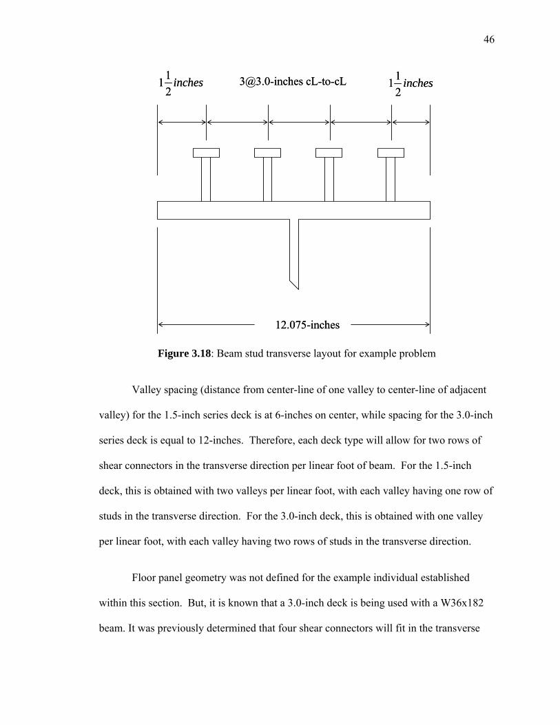
46
12.075-inches
[email protected] cL-to-cL112
inches 112
inches
12.075-inches
[email protected] cL-to-cL112
inches 112
inches
Figure 3.18: Beam stud transverse layout for example problem
Valley spacing (distance from center-line of one valley to center-line of adjacent
valley) for the 1.5-inch series deck is at 6-inches on center, while spacing for the 3.0-inch
series deck is equal to 12-inches. Therefore, each deck type will allow for two rows of
shear connectors in the transverse direction per linear foot of beam. For the 1.5-inch
deck, this is obtained with two valleys per linear foot, with each valley having one row of
studs in the transverse direction. For the 3.0-inch deck, this is obtained with one valley
per linear foot, with each valley having two rows of studs in the transverse direction.
Floor panel geometry was not defined for the example individual established
within this section. But, it is known that a 3.0-inch deck is being used with a W36x182
beam. It was previously determined that four shear connectors will fit in the transverse

47
direction at each valley location along the 12.075-inch flange. Also, it was determined
that two rows could be used in the transverse direction in each rib valley. So, this
individual can fit 4 * 2 = 8 shear connectors in every foot of beam length. So, if the beam
length is 40-feet, then 320 shear connectors could be accommodated. Following the
calculation provided in Figure 4.17, [ ( 40 / 2 ) * 2 * 4 ] = 160 shear connectors should fit
per half beam for a total of 320. The actual number of shear studs per half beam, 124, is
obtained from the beam stud gene and was decoded using the pseudo-code of Figure
3.16. This number is less than the maximum number of shear studs per half beam, 160,
so no modifications are made and the gene_repair sub-function is not used. If
modifications are required, the pseudo-code of Figure 3.19 would be used to alter the
value in nStud and launch the gene repair sub-function. The gene_repair sub-function is
used to update the genetic material in the chromosome so that it reflects the information
that has been changed within individual genes as a part of the feasibility checks
performed in decodeChromo. gene_repair is described in Section 3.5.3.
________________________________________________________________________
for indiv = 1:popSize
if nStud(indiv,1) > perHalfBeam(indiv)
nStud(indiv,1) = perHalfBeam(indiv) ;
RUN GENE REPAIR SUB-FUNCTION
end
end
________________________________________________________________________
Figure 3.19: Pseudo-code used to reduce the number of studs to the maximum number of beam studs
48
Minimum number of shear connectors per half beam
The AISC-LRFD Manual (AISC 2001) also recommends maximum shear connector
spacing limits. This recommendation leads to the second beam feasibility check in
which the individual is checked for not having enough shear studs. Pseudo-code for this
second feasibility check can be seen as Figure 3.20.
The recommended maximum shear connector spacing is the lesser of eight times
the concrete thickness above the deck rib (cover) and 36-inches (AISC 2001). But, with
a maximum possible concrete cover of 4.25-inches, the limit of 36-inches will never be
exceeded, and so, this portion of the check was not considered. This variable which
holds the value for maximum stud center-to-center spacing is titled maxBSpace. The
minimum number of shear connectors per half beam is next determined. This variable
which holds this value is titled minBStud. The calculation can be seen in Figure 3.20.
Figure 3.21 contains the pseudo-code for increasing the amount of beam studs if
the number is too low. It should be noted by the reader that if the individual has zero
beam studs, which will always be less than the minimum amount, the individual is
allowed to maintain zero studs. This is allowed because the calculations in vmCheck and
moreCheck allow for non-composite behavior. But, if any studs are used, then the
number of studs must be greater than the minimum recommended by the AISC-LRFD
manual (AISC 2001).
If the example individual established within this section (chromosome defined at
the end of the introductory section 3.3) is revisited, it can be seen that a 3.5-inch concrete
thickness is being used. The maximum spacing distance for the shear connectors would
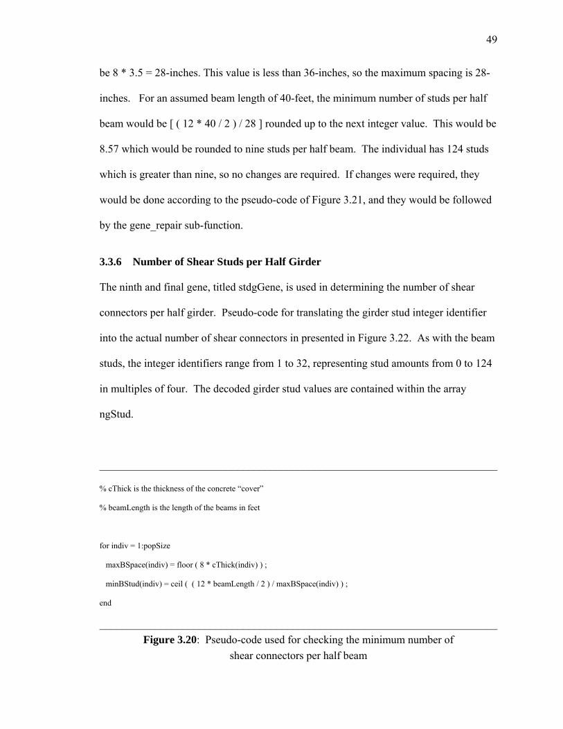
49
be 8 * 3.5 = 28-inches. This value is less than 36-inches, so the maximum spacing is 28-
inches. For an assumed beam length of 40-feet, the minimum number of studs per half
beam would be [ ( 12 * 40 / 2 ) / 28 ] rounded up to the next integer value. This would be
8.57 which would be rounded to nine studs per half beam. The individual has 124 studs
which is greater than nine, so no changes are required. If changes were required, they
would be done according to the pseudo-code of Figure 3.21, and they would be followed
by the gene_repair sub-function.
3.3.6 Number of Shear Studs per Half Girder
The ninth and final gene, titled stdgGene, is used in determining the number of shear
connectors per half girder. Pseudo-code for translating the girder stud integer identifier
into the actual number of shear connectors in presented in Figure 3.22. As with the beam
studs, the integer identifiers range from 1 to 32, representing stud amounts from 0 to 124
in multiples of four. The decoded girder stud values are contained within the array
ngStud.
________________________________________________________________________
% cThick is the thickness of the concrete “cover”
% beamLength is the length of the beams in feet
for indiv = 1:popSize
maxBSpace(indiv) = floor ( 8 * cThick(indiv) ) ;
minBStud(indiv) = ceil ( ( 12 * beamLength / 2 ) / maxBSpace(indiv) ) ;
end
________________________________________________________________________ Figure 3.20: Pseudo-code used for checking the minimum number of
shear connectors per half beam
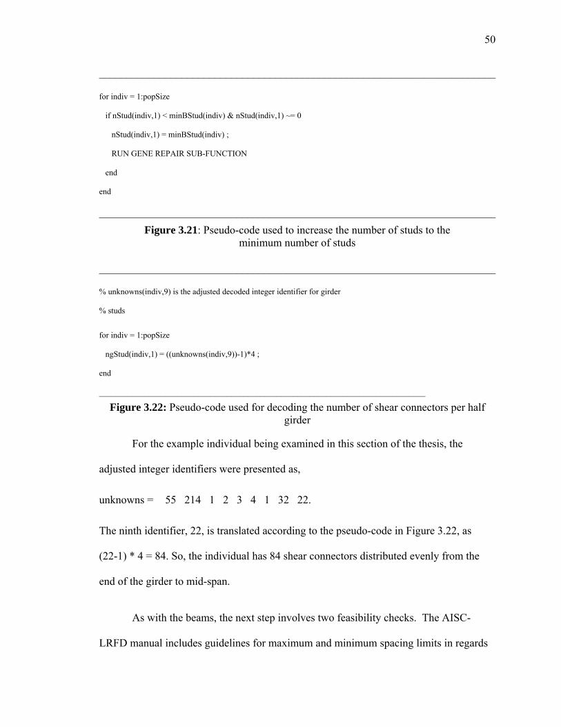
50
________________________________________________________________________
for indiv = 1:popSize
if nStud(indiv,1) < minBStud(indiv) & nStud(indiv,1) ~= 0
nStud(indiv,1) = minBStud(indiv) ;
RUN GENE REPAIR SUB-FUNCTION
end
end
________________________________________________________________________ Figure 3.21: Pseudo-code used to increase the number of studs to the
minimum number of studs
________________________________________________________________________
% unknowns(indiv,9) is the adjusted decoded integer identifier for girder
% studs
for indiv = 1:popSize
ngStud(indiv,1) = ((unknowns(indiv,9))-1)*4 ;
end
_______________________________________________________________________________
Figure 3.22: Pseudo-code used for decoding the number of shear connectors per half girder
For the example individual being examined in this section of the thesis, the
adjusted integer identifiers were presented as,
unknowns = 55 214 1 2 3 4 1 32 22.
The ninth identifier, 22, is translated according to the pseudo-code in Figure 3.22, as
(22-1) * 4 = 84. So, the individual has 84 shear connectors distributed evenly from the
end of the girder to mid-span.
As with the beams, the next step involves two feasibility checks. The AISC-
LRFD manual includes guidelines for maximum and minimum spacing limits in regards
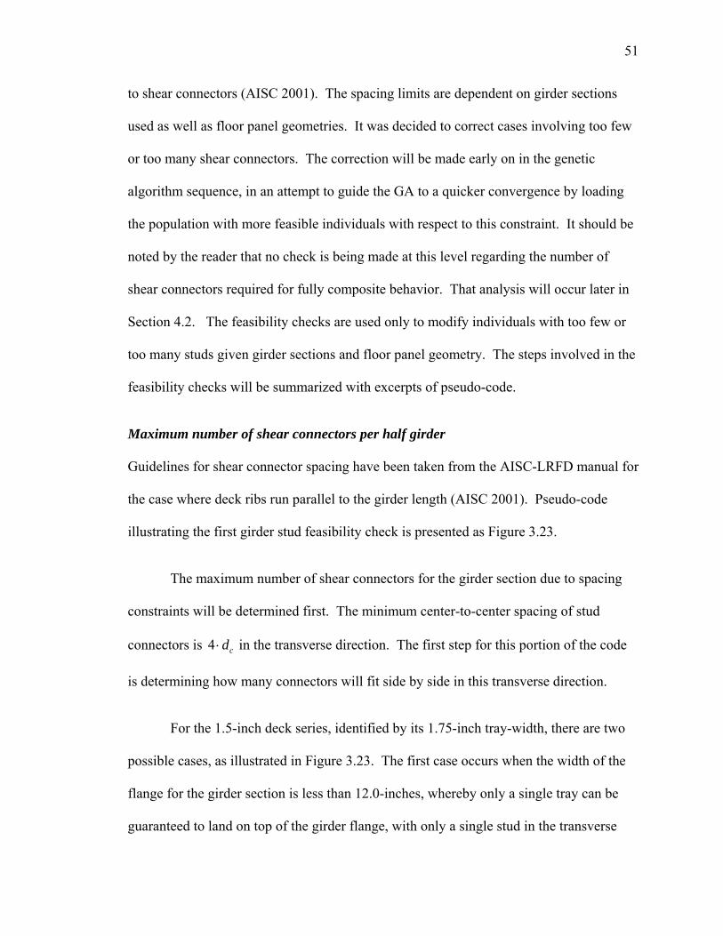
51
to shear connectors (AISC 2001). The spacing limits are dependent on girder sections
used as well as floor panel geometries. It was decided to correct cases involving too few
or too many shear connectors. The correction will be made early on in the genetic
algorithm sequence, in an attempt to guide the GA to a quicker convergence by loading
the population with more feasible individuals with respect to this constraint. It should be
noted by the reader that no check is being made at this level regarding the number of
shear connectors required for fully composite behavior. That analysis will occur later in
Section 4.2. The feasibility checks are used only to modify individuals with too few or
too many studs given girder sections and floor panel geometry. The steps involved in the
feasibility checks will be summarized with excerpts of pseudo-code.
Maximum number of shear connectors per half girder
Guidelines for shear connector spacing have been taken from the AISC-LRFD manual for
the case where deck ribs run parallel to the girder length (AISC 2001). Pseudo-code
illustrating the first girder stud feasibility check is presented as Figure 3.23.
The maximum number of shear connectors for the girder section due to spacing
constraints will be determined first. The minimum center-to-center spacing of stud
connectors is 4 cd⋅ in the transverse direction. The first step for this portion of the code
is determining how many connectors will fit side by side in this transverse direction.
For the 1.5-inch deck series, identified by its 1.75-inch tray-width, there are two
possible cases, as illustrated in Figure 3.23. The first case occurs when the width of the
flange for the girder section is less than 12.0-inches, whereby only a single tray can be
guaranteed to land on top of the girder flange, with only a single stud in the transverse

52
direction. In this case, the value for rows is one. The second case occurs when the width
of the girder flange is greater than 12.0-inches, guaranteeing that two valleys will land on
top of the girder flange. Again, with only a single shear connector per valley, the amount
of studs in the transverse direction, and the value for rows, is two.
For the 3.0-inch deck series, there are also two possible cases, as illustrated in
Figure 3.23. It will not be possible, however, to guarantee that two valleys will ever land
on top of the same girder flange. For this to happen, the girder flange would have to be at
least 24-inches wide. The maximum flange width for a section in the AISC-LRFD
Database of Wide-Flange Shapes is approximately 18-inches. So, that case will not be
considered.
The first case that will be considered is for shear connector diameter of 1-inch or
more. Minimum center-to-center spacing in the direction transverse to the girder would
be four diameters or 4-inches. An extra diameter would also have to be added for the half
stud on each side that extended past the center-to-center distance, for a total of 5-inches.
The tray width for the 3.0-inch deck is only 4.75-inches, so in this case, the amount of
shear connectors that would fit transverse to the girder is one. The value for the variable
rows would be one. The second case is for shear connector diameters of less than 1-
inch. For all of these sizes, the maximum total width ever needed would be 4.375-inches.
This would allow two shear connectors transverse to the girder for all cases with a 3.0-
inch deck and stud diameters less than 1-inch. The value for rows would be two.
The example individual established earlier in this section will be examined in
regards to this feasibility check. The chromosome of this example individual is defined
at the end of the introductory section 4.3. The individual used a W12x230 girder, with a
53
flange width equal to 12.9-inches, and a 3.0-inch deck series. According to the
calculation for rows presented in Figure 3.23, and assuming a stud diameter of 0.75-
inches, the individual would have two studs in the direction transverse to the girder.
The next step is to determine the maximum number of studs that will fit per half
girder. The variable for this value is perHalfGird and the calculation is shown in Figure
3.23. The calculation involves multiplying the amount of studs in the transverse
direction by the number of studs that would fit longitudinally at a minimum spacing.
The minimum center-to-center spacing for studs in the longitudinal direction given deck
ribs that run parallel to the girder is 6 cd⋅ .
For the example individual who is being examined in this section (chromosome
defined at the end of the introductory section 3.3), and with an assumed girder length of
30-feet (this fits with the previous feasibility check for deck clear span), the maximum
number of shear studs per half girder would be equal to two times the quantity [(30/2)*12
/ (6*0.75)] rounded down to the next integer value. This would equal a maximum of 80
studs per half girder. Our individual exceeds this limit, with 84, and so the value of the
variable ngStud needs to be altered and the gene subjected to gene_repair. The steps for
this process are outlined in the pseudo-code of Figure 3.24.
Minimum number of shear connectors per half girder
AISC-LRFD recommends maximum shear connector spacing limits for the case where
deck ribs runs parallel to the girder length (AISC 2001). This recommendation leads to a
minimum amount of shear connectors for half the girder span, and this calculation is the
54
second feasibility check for this section. Pseudo-code for this check is included in Figure
3.25.
The recommended maximum shear connector spacing is the lesser of 8 ct⋅ and 36-
inches. But, with a maximum concrete cover of 4.25-inches, the 36-inch limit would
never be exceeded, and so it was ignored. The variable which holds the value for the
maximum center-to-center stud spacing is maxGSpace. The minimum number of shear
connectors allowed per half girder is next determined. The variable which holds this
value is titled minGStud. The calculation can be seen in Figure 3.25.
Figure 3.26 contains the pseudo-code for increasing the amount of girder studs if
the number is too low. It should be noted that if the individual has zero girder studs,
which will always be less than the minimum amount given spacing constraints, the
individual is allowed to maintain zero studs. This is done because the calculations in
vmCheck allow for non-composite girders. Also, gene_repair would again be used to
correct the original chromosome.
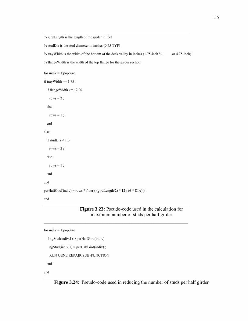
55
_______________________________________________________________________________ % girdLength is the length of the girder in feet
% studDia is the stud diameter in inches (0.75 TYP)
% trayWidth is the width of the bottom of the deck valley in inches (1.75-inch % or 4.75-inch)
% flangeWidth is the width of the top flange for the girder section
for indiv = 1:popSize
if trayWidth == 1.75
if flangeWidth >= 12.00
rows = 2 ;
else
rows = 1 ;
end
else
if studDia < 1.0
rows = 2 ;
else
rows = 1 ;
end
end
perHalfGird(indiv) = rows * floor ( (girdLength/2) * 12 / (6 * DIA) ) ;
end _______________________________________________________________________________
Figure 3.23: Pseudo-code used in the calculation for maximum number of studs per half girder
_______________________________________________________________________________
for indiv = 1:popSize
if ngStud(indiv,1) > perHalfGird(indiv)
ngStud(indiv,1) = perHalfGird(indiv) ;
RUN GENE REPAIR SUB-FUNCTION
end
end _______________________________________________________________________________
Figure 3.24: Pseudo-code used in reducing the number of studs per half girder
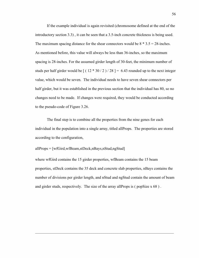
56
If the example individual is again revisited (chromosome defined at the end of the
introductory section 3.3) , it can be seen that a 3.5-inch concrete thickness is being used.
The maximum spacing distance for the shear connectors would be 8 * 3.5 = 28-inches.
As mentioned before, this value will always be less than 36-inches, so the maximum
spacing is 28-inches. For the assumed girder length of 30-feet, the minimum number of
studs per half girder would be [ ( 12 * 30 / 2 ) / 28 ] = 6.43 rounded up to the next integer
value, which would be seven. The individual needs to have seven shear connectors per
half girder, but it was established in the previous section that the individual has 80, so no
changes need to be made. If changes were required, they would be conducted according
to the pseudo-code of Figure 3.26.
The final step is to combine all the properties from the nine genes for each
individual in the population into a single array, titled allProps. The properties are stored
according to the configuration,
allProps = [wfGird,wfBeam,stDeck,nBays,nStud,ngStud]
where wfGird contains the 15 girder properties, wfBeam contains the 15 beam
properties, stDeck contains the 35 deck and concrete slab properties, nBays contains the
number of divisions per girder length, and nStud and ngStud contain the amount of beam
and girder studs, respectively. The size of the array allProps is ( popSize x 68 ) .
_______________________________________________________________________
57
% cThick is the thickness of the concrete above deck ribs in inches
% girdLength is the length of the girder in feet
for indiv = 1:popSize
maxGSpace(indiv) = floor ( 8 * cThick(indiv) ) ;
minGStud(indiv) = ceil ( ( 12 * girdLength / 2 ) / maxGSpace(indiv) ) ;
end
_______________________________________________________________________________
Figure 3.25: Pseudo-code used in calculating the minimum number of studs per half girder
_______________________________________________________________________________
for indiv = 1:popSize
if ngStud(indiv,1) < minGStud(indiv) & ngStud(indiv,1) ~= 0
ngStud(indiv,1) = minGStud(indiv) ;
RUN GENE REPAIR SUB-FUNCTION
end
end
_______________________________________________________________________________
Figure 3.26: Pseudo-code used to increase the number of studs per half girder
3.4 FUNCTION: eliminate.m

58
The function eliminate.m is used directly after the gather operation. eliminate is used to
remove duplicate solutions from the collection of feasible individuals. Feasible
individuals were defined as solutions to the original floor framing problem with penalty
violations less than 1.05. Duplicate individuals are common within the GA. It is often
very easy for highly-fit individuals to replicate and begin to dominate the population.
The removal of these solutions is not essential to the function of the GA, but doing so
does make results easier to analyze. The steps required to execute the eliminate operation
will be discussed. MATLAB code for the function is presented in Figure 3.27.
The array containing the feasible individuals, vibe_chromo, first has all of its
elements changed from number elements to string elements. This step is completed using
MATLAB’s num2str, or number to string converter. The step is necessary in order to use
another one of MATLAB’s functions, as will be described later. A new array,
unique_vibe_chromo, is created and will be used to hold a single copy of each individual
in the population. To begin the procedure, the first individual from vibe_chromo in
placed in the new array. Next, single individuals from the original array are examined. A
check is made to see if a duplicate solution exists in unique_vibe_chromo. If a solution
already exists in the new array, nothing happens, but if no such solution exists, the
solution will be added. The process continues until all individuals from the original array
have been checked.
The method of checking to see if a duplicate solution exists in the new array is
accomplished with MATLAB’s strmatch, or string match function. strmatch searches for
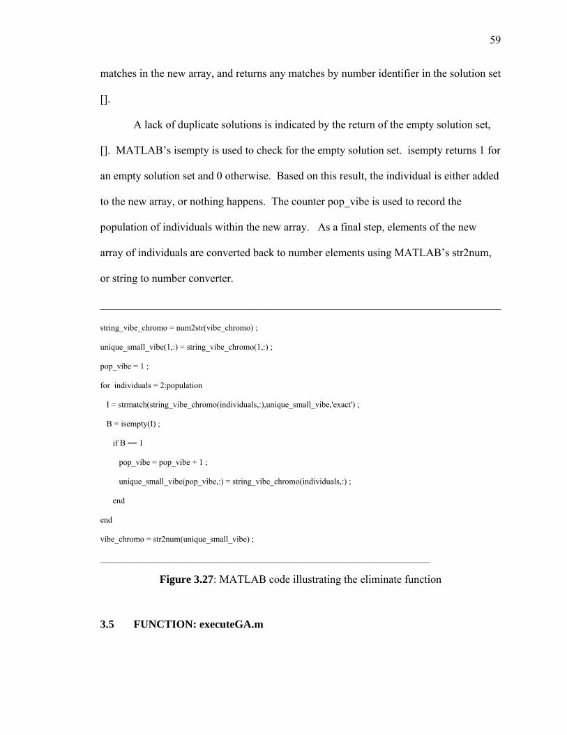
59
matches in the new array, and returns any matches by number identifier in the solution set
[].
A lack of duplicate solutions is indicated by the return of the empty solution set,
[]. MATLAB’s isempty is used to check for the empty solution set. isempty returns 1 for
an empty solution set and 0 otherwise. Based on this result, the individual is either added
to the new array, or nothing happens. The counter pop_vibe is used to record the
population of individuals within the new array. As a final step, elements of the new
array of individuals are converted back to number elements using MATLAB’s str2num,
or string to number converter.
________________________________________________________________________
string_vibe_chromo = num2str(vibe_chromo) ;
unique_small_vibe(1,:) = string_vibe_chromo(1,:) ;
pop_vibe = 1 ;
for individuals = 2:population
I = strmatch(string_vibe_chromo(individuals,:),unique_small_vibe,'exact') ;
B = isempty(I) ;
if B == 1
pop_vibe = pop_vibe + 1 ;
unique_small_vibe(pop_vibe,:) = string_vibe_chromo(individuals,:) ;
end
end
vibe_chromo = str2num(unique_small_vibe) ;
_______________________________________________________________________________
Figure 3.27: MATLAB code illustrating the eliminate function
3.5 FUNCTION: executeGA.m

60
This function is the controller used in sequencing different elements of the genetic
algorithm. It controls multiple functions that are used as the GA cycles from generation
to generation. Two versions of this file will be discussed in this section. One version
drives the single-objective GA, and the other controls the multi-objective GA using
maximin fitness evaluation (Balling, et al 2001).
The single-objective version of the GA differs from the multi-objective version in
both the location in which the floor panel acceleration values are computed and the
definition of fitness. The single-objective version, described below, does not compute
floor panel accelerations for every generation. It computes them at the end of the
evolution on a collection of feasible individuals. These feasible individuals are collected
from the final generations of several different GA runs. In comparison, the multi–
objective GA uses floor panel accelerations in each generation of individuals as a part of
the maximin fitness evaluation.
3.5.1 Single-Objective Genetic Algorithm
The main steps involved in running the GA will be discussed in the order that they are
used. The reader is referred to Figures 3.28 and 3.29 for a visual representation of the
GA functions, including sequence and purpose.
With user inputs and the problem definition already established, the function
executeGA.m begins by creating the initial population of individuals through randomly
assigned binary digits which will be checked and evaluated later. The mutation operation
is performed next, which serves to randomly alter a certain percentage of each
chromosome’s digits. The mutation operator does not act on the initial generation. The

61
next step involves decoding the binary information located within the chromosome first
into integer designations, and then into useable problem data.
The function allChecks.m is next utilized (see Section 3.1 for more information).
This function calls two sub-functions, vmCheck.m and moreChecks.m. vmCheck
computes shear and moment states from known loading conditions as well as shear and
moment capacities for the beams and girders of each individual in the population.
moreChecks examines additional strength and deflection states, that include end use as
well as construction conditions. More information regarding vmCheck.m and
moreCheck.m can be found in Sections 3.16 and 3.12, respectively. If the results for an
individual are not satisfactory with established standards, penalty functions are created
which will increase the individual’s total panel cost later in the GA. More information on
the calculation of individual penalties can be found in Section 3.1.2.
The next function to be used, findFitness.m, evaluates an individual’s fitness
based solely on total panel cost multiplied by penalty functions. Total panel cost includes
costs for structural steel, concrete for slabs, and steel decking as well as shear studs. More
information regarding the calculation of fitness can be found in Section 3.6. The
population is then ranked based on this computation of total cost. The population is
subsequently reordered from minimal cost to maximum cost. More information on the
ranking procedure can be found in Section 3.14.
The selection.m function chooses individuals to serve as the genetic source for
new offspring in the subsequent generation. Information relating to the selection
procedure can be found in Section 3.15. Individuals are chosen based on a population

62
partitioning method (Camp, et al 1999). The selection function also permits a certain
percentage of the most-fit individuals to pass on unaltered to the next generation. The
next function, crossover.m, combines the genetic material of the two chosen genetic
sources in order to form a new individual. The crossover method is known as single-
point crossover. More information regarding the crossover procedure can be found in
Section 3.2.
At this point, a new population has been created, and the first generation has been
completed. A looping procedure is begun, whereby the functions mutation.m,
decodeChromo.m, allChecks.m, findFitness.m, ranking.m, selection.m, and crossover.m
will be repeated for a desired number of generations. This repeating loops are illustrated
by the flow charts in Figures 3.28 and 3.29. When all generations have been run, the GA
will present a group of the most-fit individuals which represent very good solutions to the
problem. It should be noted that the GA does not find the absolute best solution to any
problem, but rather presents a collection of very good solutions.
Now that one run of the GA has been completed, the option to repeat the entire
GA is presented to the user. The GA can be repeated up to ten times total. This step is
recommended, as it provides a good method for analyzing other related solutions. Once
all the GA runs have been completed, the function gather.m is utilized. gather.m collects
all feasible individuals from the final generation of each GA run. Feasible individuals are
defined as individuals whose penalty function product is less than 1.05. More
information regarding the gather procedure in included in Section 3.8.
63
The function eliminate.m will then remove any duplicate solutions from this
group. More information regarding the eliminate procedure in included in Section 3.4.
Duplicate solutions are very common within the evolutionary algorithm, as very fit
individuals tend to reproduce and can dominate the population in later generations. The
unique solutions are then passed through the function decodeChromo and their binary
information is decoded one last time. More information regarding the decodeChromo
procedure in included in Section 3.3. At this point in the GA, the function floorVib.m is
used to evaluate the vibration performance of each individual in the population. To
finish, the GA presents five MATLAB plots and creates two output text files to
communicate results to the user. The five plots show convergence trajectories, natural
frequency of vibration (two views), and acceleration due to walking vibration with
respect to the acceleration of gravity (two views). The text file, output.txt, provides the
user with useful information for individuals in the final generation of each GA run. The
text file, results.txt, provides information about individual solutions that the program user
is able to choose.
3.5.2 Multi-Objective Genetic Algorithm
The second version of the genetic algorithm, which uses maximin fitness evaluation
(Balling, et al 2001), involves fewer steps. The principal difference in this version is the
calculation of the vibration performance within each generation of the evolutionary
algorithm. A flow chart showing the steps involved in this version in included in Figure
3.30. The visual representation includes function sequencing as well as purpose.
As before, once user input and the problem definition are established, the function
executeGA.m begins by creating the initial population of individuals. The functions
64
mutation.m, decodeChromo.m, and allChecks.m again follow. The difference in this
version of the GA arises within the function findFitness.m. Previously, fitness was
based solely on cost. In this version, fitness is based on both cost and vibration
performance, and each must be determined. More information on the findFitness
procedure in included in Section 3.6. Total adjusted panel cost is developed within
findFitness.m, but floor system accelerations must be determined using the sub-function
floorVib.m. With total adjusted cost and floor system accelerations computed, the
function maximin.m is used to determine the fitness of each individual. The maximin
fitness statement is described in Section 3.11.
With fitness now determined, the functions ranking.m, selection.m, and
crossover.m, are again utilized. A loop is again used to repeat this process for a desired
number of generations. No repeat runs are performed. The GA is completed with the
presentation to the user of eight MATLAB plots and an output text file. The plots show
color-coded maximin fitness values after the initial and first generations, as well as
Pareto-based plots following the first, fifth, tenth, twentieth, thirtieth, and fortieth
generations.
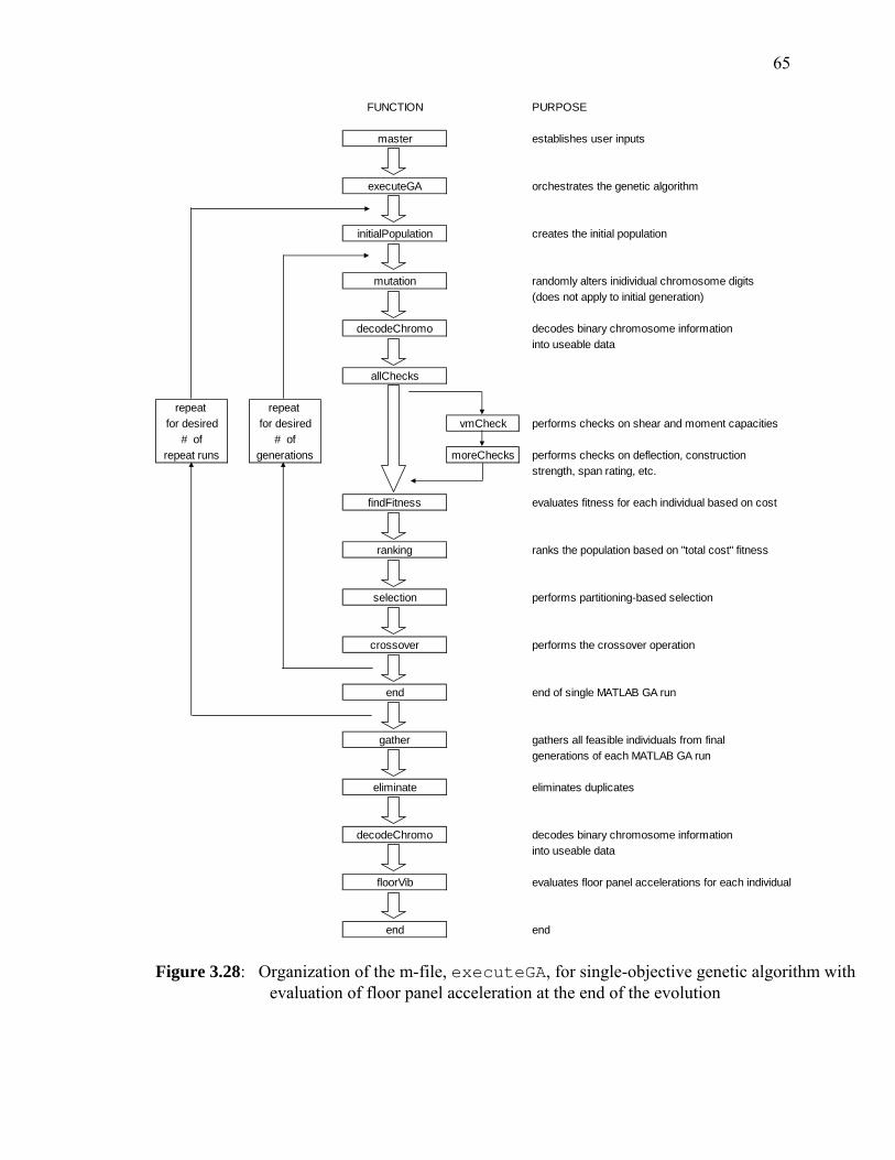
65
FUNCTION PURPOSE
master establishes user inputs
executeGA orchestrates the genetic algorithm
initialPopulation creates the initial population
mutation randomly alters inidividual chromosome digits(does not apply to initial generation)
decodeChromo decodes binary chromosome information into useable data
allChecks
repeat repeat for desired for desired vmCheck performs checks on shear and moment capacities
# of # ofrepeat runs generations moreChecks performs checks on deflection, construction
strength, span rating, etc.
findFitness evaluates fitness for each individual based on cost
ranking ranks the population based on "total cost" fitness
selection performs partitioning-based selection
crossover performs the crossover operation
end end of single MATLAB GA run
gather gathers all feasible individuals from final generations of each MATLAB GA run
eliminate eliminates duplicates
decodeChromo decodes binary chromosome information into useable data
floorVib evaluates floor panel accelerations for each individual
end end Figure 3.28: Organization of the m-file, executeGA, for single-objective genetic algorithm with evaluation of floor panel acceleration at the end of the evolution
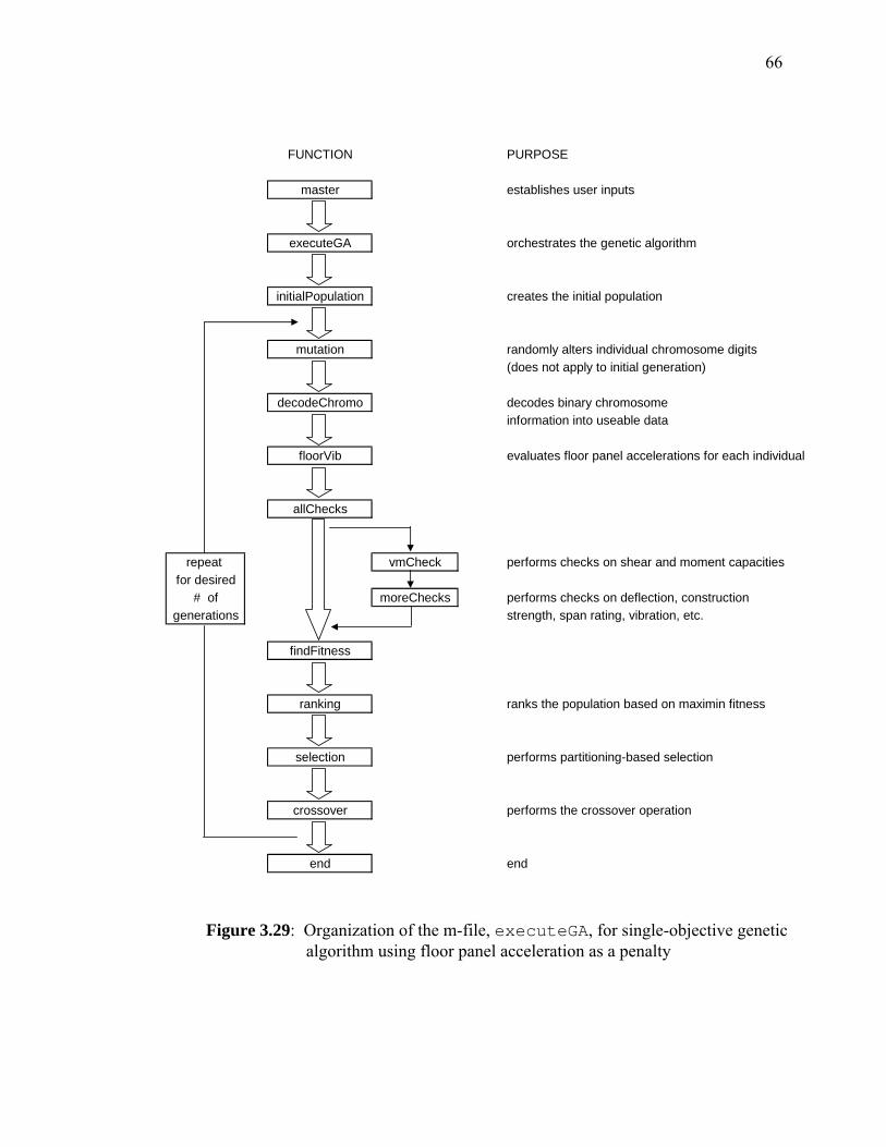
66
FUNCTION PURPOSE
master establishes user inputs
executeGA orchestrates the genetic algorithm
initialPopulation creates the initial population
mutation randomly alters individual chromosome digits(does not apply to initial generation)
decodeChromo decodes binary chromosome information into useable data
floorVib evaluates floor panel accelerations for each individual
allChecks
repeat vmCheck performs checks on shear and moment capacitiesfor desired
# of moreChecks performs checks on deflection, constructiongenerations strength, span rating, vibration, etc.
findFitness
ranking ranks the population based on maximin fitness
selection performs partitioning-based selection
crossover performs the crossover operation
end end
Figure 3.29: Organization of the m-file, executeGA, for single-objective genetic algorithm using floor panel acceleration as a penalty
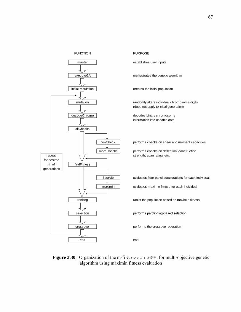
67
FUNCTION PURPOSE
master establishes user inputs
executeGA orchestrates the genetic algorithm
initialPopulation creates the initial population
mutation randomly alters individual chromosome digits(does not apply to initial generation)
decodeChromo decodes binary chromosome information into useable data
allChecks
vmCheck performs checks on shear and moment capacities
moreChecks performs checks on deflection, constructionrepeat strength, span rating, etc.
for desired# of findFitness
generations
floorVib evaluates floor panel accelerations for each individual
maximin evaluates maximin fitness for each individual
ranking ranks the population based on maximin fitness
selection performs partitioning-based selection
crossover performs the crossover operation
end end
Figure 3.30: Organization of the m-file, executeGA, for multi-objective genetic algorithm using maximin fitness evaluation
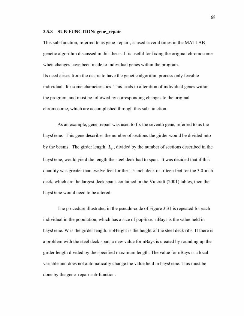
68
3.5.3 SUB-FUNCTION: gene_repair
This sub-function, referred to as gene_repair , is used several times in the MATLAB
genetic algorithm discussed in this thesis. It is useful for fixing the original chromosome
when changes have been made to individual genes within the program.
Its need arises from the desire to have the genetic algorithm process only feasible
individuals for some characteristics. This leads to alteration of individual genes within
the program, and must be followed by corresponding changes to the original
chromosome, which are accomplished through this sub-function.
As an example, gene_repair was used to fix the seventh gene, referred to as the
baysGene. This gene describes the number of sections the girder would be divided into
by the beams. The girder length, gL , divided by the number of sections described in the
baysGene, would yield the length the steel deck had to span. It was decided that if this
quantity was greater than twelve feet for the 1.5-inch deck or fifteen feet for the 3.0-inch
deck, which are the largest deck spans contained in the Vulcraft (2001) tables, then the
baysGene would need to be altered.
The procedure illustrated in the pseudo-code of Figure 3.31 is repeated for each
individual in the population, which has a size of popSize. nBays is the value held in
baysGene. W is the girder length. ribHeight is the height of the steel deck ribs. If there is
a problem with the steel deck span, a new value for nBays is created by rounding up the
girder length divided by the specified maximum length. The value for nBays is a local
variable and does not automatically change the value held in baysGene. This must be
done by the gene_repair sub-function.
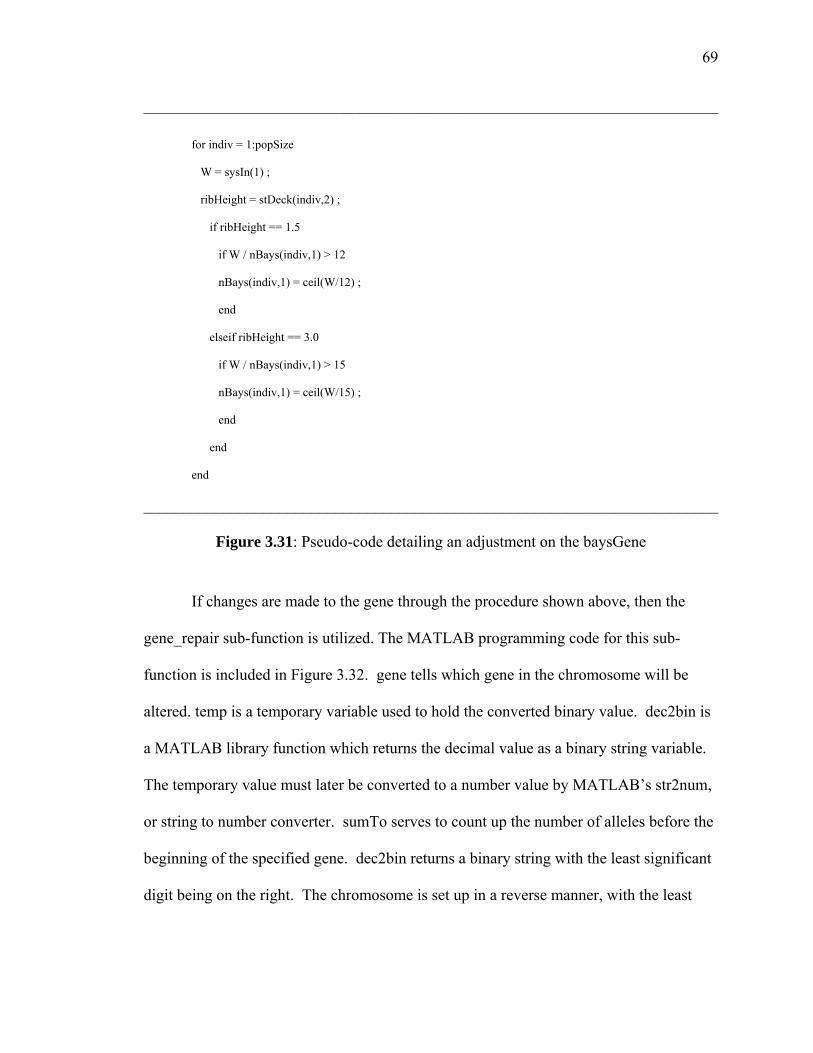
69
________________________________________________________________________ for indiv = 1:popSize
W = sysIn(1) ;
ribHeight = stDeck(indiv,2) ;
if ribHeight == 1.5
if W / nBays(indiv,1) > 12
nBays(indiv,1) = ceil(W/12) ;
end
elseif ribHeight == 3.0
if W / nBays(indiv,1) > 15
nBays(indiv,1) = ceil(W/15) ;
end
end
end
________________________________________________________________________
Figure 3.31: Pseudo-code detailing an adjustment on the baysGene
If changes are made to the gene through the procedure shown above, then the
gene_repair sub-function is utilized. The MATLAB programming code for this sub-
function is included in Figure 3.32. gene tells which gene in the chromosome will be
altered. temp is a temporary variable used to hold the converted binary value. dec2bin is
a MATLAB library function which returns the decimal value as a binary string variable.
The temporary value must later be converted to a number value by MATLAB’s str2num,
or string to number converter. sumTo serves to count up the number of alleles before the
beginning of the specified gene. dec2bin returns a binary string with the least significant
digit being on the right. The chromosome is set up in a reverse manner, with the least

70
significant digit being on the left, so the rest of the programming serves to fill the original
chromosome with the new binary number in a reverse way.
________________________________________________________________________
gene = 7 ;
temp = dec2bin( ( nBays(indiv,1) ) - 2 , geneLength(gene) ) ;
sumTo = 0 ;
for i = 1: (gene-1)
sumTo = sumTo + geneLength(i) ;
end
for allele = 1:geneLength(gene)
temp(allele) = str2num( temp(allele) ) ;
end
for allele = 1:geneLength(gene)
chromosome(indiv,(sumTo+allele)) = temp(geneLength(gene)-allele+1);
end
________________________________________________________________________
Figure 3.32: MATLAB code describing the gene repair sub-function
3.6 FUNCTION: findFitness.m
The function findFitness is used to generate a quantitative measure of how well each
individual solves the original floor framing problem. (The problem is described in detail
in Section 1.3.) This value is referred to as the fitness for the individual. There are two
slightly different versions of the function findFitness which will be described in this
section. In the first version, a single-objective fitness statement is utilized. The fitness of
each individual is based on one quantity, which is the total adjusted floor panel cost. The
71
cost is described as adjusted because the cost value is multiplied by the product of the
penalty factors. For more information on the penalty factors, see Section 3.1.2.
The second version of the function findFitness is used within the multi-objective
version of the genetic algorithm. In this version, the fitness value for each individual is
based on both total adjusted panel cost and adjusted floor panel acceleration. The fitness
is calculated using a maximin fitness evaluation process developed by the authors in
(Balling, et al 2001). For more information on maximin fitness evaluation, see Section
3.11.
3.6.1 MATLAB Code Used in Both Versions
Before beginning with the evaluation of an individual’s fitness, all relevant problem data
must be imported into the findFitness function. This process is illustrated by the pseudo-
code shown in Figure 3.33. Relevant data including the weight of beam, girder, and deck
sections, the number of studs for the beam and girder, deck height, concrete type and
thickness, and the number of bays is imported from the array allProps which was created
in decodeChromo. Computed values for total concrete thickness and square footage of
the floor panel are next calculated. Beam and girder lengths are obtained from the array
sysIn which was created in master. Cost values for all the structural components are
obtained from the array costIn which was also created in master.
The next process, as illustrated by the pseudo-code of Figure 3.34, is to determine
the total volume of concrete required for each individual solution. Knowing the number
of squares, or hundreds of square feet, required given the floor panel geometry, the
volume of concrete can be calculated using values from the Vulcraft Steel Roof and Floor
72
Deck manual (Vulcraft 2001). The mentioned values are theoretical volumes of concrete
in cubic yards per square. The appropriate values are obtained using a logic statement,
as can be seen in the pseudo-code of Figure 3.34. The value for cubic yards per square is
held in the variable yardsPerSq. It should be noted by the reader that although volumes
of concrete are the same regardless of concrete type, that different sections of the logic
statement had to be used because of differing concrete thicknesses. The light-weight
concrete thicknesses were 2.5-inch, 3-inch, 3.5-inch, and 4.25-inch, while the normal
weight concrete thicknesses were 2.5-inch, 3-inch, 3.5-inch, and 4-inch.
After the correct value is chosen for yardsPerSq, the total volume of concrete for
each individual is easily computed as yardsPerSq * squares. The value for total volume
is held in either the variable yardsOfLW or the variable yardsOfNW, depending on the
concrete type.
As illustrated in Figure 3.35, the next step is to compute the total adjusted panel
cost. Calculations are made for beamCost, girdCost, deckCost, LWcost, NWcost,
beamStudCost, and girdStudCost. The structural component costs are added and stored as
the variable with name sum1. The adjusted total floor panel cost is computed by
multiplying sum1 with phiProd and phiProd2. phiProd and phiProd2 represent the
penalty functions as defined in Section 3.1.2. If none of the strength and deflection
constraints are violated, the product of phiProd and phiProd2 is simply 1.0, and the
adjusted total floor panel cost is simply the value held in sum1.
It should be noted that only one girder and the amount of beams equal to the
number of bays, or divisions per girder length, are included in calculations for the total
73
adjusted panel cost. This was done to create a situation where the total cost for a number
of floor panels could be calculated by multiplying the cost per panel by the number of
panels. It is assumed that adjacent panels will share the cost of the common girder or
common beam by which they are connected. Thus, each panel will assume cost for half
of the girder on each end, making for 2 * ½ = 1 full girder. A similar approach was used
for the beams.
3.6.2 Single-Objective Version
For the single objective version of the function findFitness, the total adjusted panel cost
serves as the fitness measure, and no additional steps are required. As illustrated in the
pseudo-code of Figure 3.36, results are reported back to executeGA in the array
cost_column, which is of size (popSize x 2). The first column holds the fitness value,
which is adjusted total cost. The second column holds a marker which identifies the
individual. This marker will be used later during the ranking function.
________________________________________________________________________
DATA TAKEN FROM THE ARRAY allProps (see FUNCTION: decodeChromo)
% wtBeams is the weight of the beams in pounds per foot
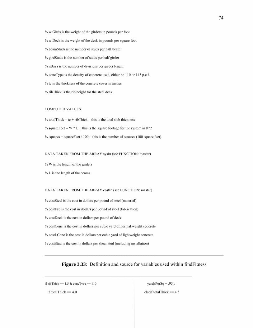
74
% wtGirds is the weight of the girders in pounds per foot
% wtDeck is the weight of the deck in pounds per square foot
% beamStuds is the number of studs per half beam
% girdStuds is the number of studs per half girder
% nBays is the number of divisions per girder length
% concType is the density of concrete used, either be 110 or 145 p.c.f.
% tc is the thickness of the concrete cover in inches
% ribThick is the rib height for the steel deck
COMPUTED VALUES
% totalThick = tc + ribThick ; this is the total slab thickness
% squareFeet = W * L ; this is the square footage for the system in ft^2
% squares = squareFeet / 100 ; this is the number of squares (100 square feet)
DATA TAKEN FROM THE ARRAY sysIn (see FUNCTION: master)
% W is the length of the girders
% L is the length of the beams
DATA TAKEN FROM THE ARRAY costIn (see FUNCTION: master)
% costSteel is the cost in dollars per pound of steel (material)
% costFab is the cost in dollars per pound of steel (fabrication)
% costDeck is the cost in dollars per pound of deck
% costConc is the cost in dollars per cubic yard of normal weight concrete
% costLConc is the cost in dollars per cubic yard of lightweight concrete
% costStud is the cost in dollars per shear stud (including installation)
________________________________________________________________________
Figure 3.33: Definition and source for variables used within findFitness
_______________________________________________________________________________
if ribThick == 1.5 & concType == 110
if totalThick == 4.0
yardsPerSq = .93 ;
elseif totalThick == 4.5
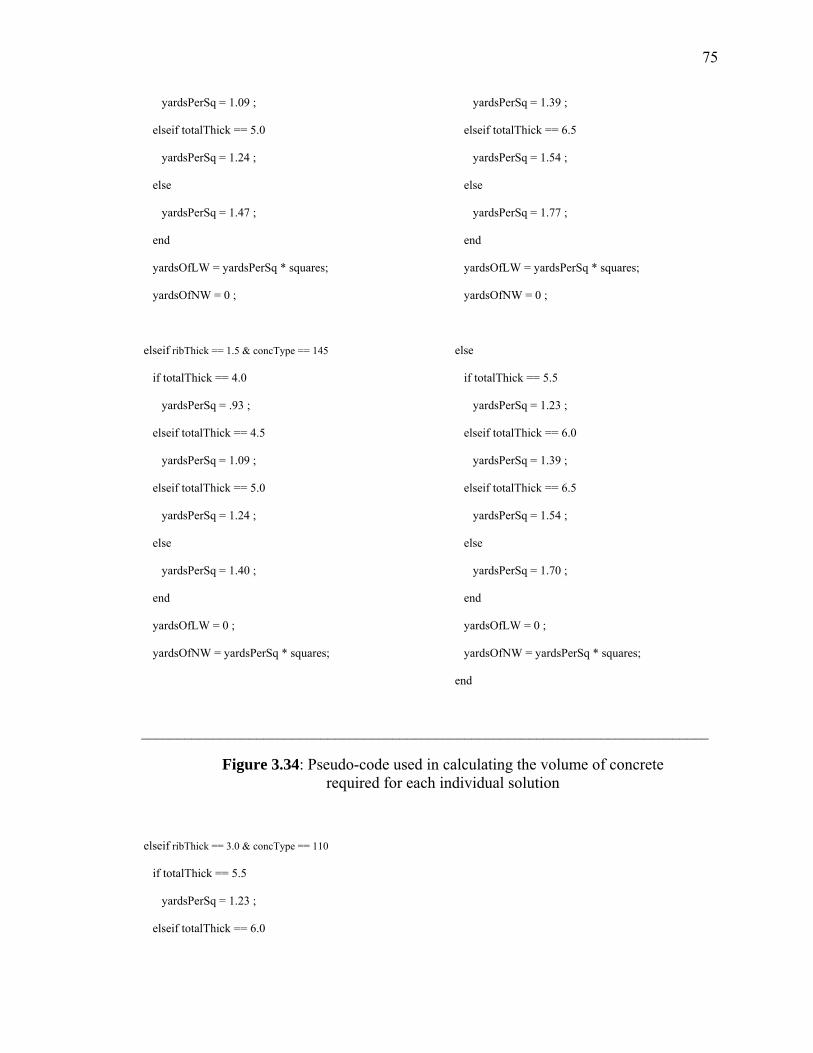
75
yardsPerSq = 1.09 ;
elseif totalThick == 5.0
yardsPerSq = 1.24 ;
else
yardsPerSq = 1.47 ;
end
yardsOfLW = yardsPerSq * squares;
yardsOfNW = 0 ;
elseif ribThick == 1.5 & concType == 145
if totalThick == 4.0
yardsPerSq = .93 ;
elseif totalThick == 4.5
yardsPerSq = 1.09 ;
elseif totalThick == 5.0
yardsPerSq = 1.24 ;
else
yardsPerSq = 1.40 ;
end
yardsOfLW = 0 ;
yardsOfNW = yardsPerSq * squares;
elseif ribThick == 3.0 & concType == 110
if totalThick == 5.5
yardsPerSq = 1.23 ;
elseif totalThick == 6.0
yardsPerSq = 1.39 ;
elseif totalThick == 6.5
yardsPerSq = 1.54 ;
else
yardsPerSq = 1.77 ;
end
yardsOfLW = yardsPerSq * squares;
yardsOfNW = 0 ;
else
if totalThick == 5.5
yardsPerSq = 1.23 ;
elseif totalThick == 6.0
yardsPerSq = 1.39 ;
elseif totalThick == 6.5
yardsPerSq = 1.54 ;
else
yardsPerSq = 1.70 ;
end
yardsOfLW = 0 ;
yardsOfNW = yardsPerSq * squares;
end
_______________________________________________________________________________
Figure 3.34: Pseudo-code used in calculating the volume of concrete required for each individual solution

76
_______________________________________________________________________________
% phiProd is the product of the first four penalty functions from vmCheck
% phiProd2 is the product of the remaining eight penalty functions from
% moreCheck
beamCost(indiv) = nBays * L * wtBeams * (costSteel + costFab) ;
girdCost(indiv) = W * wtGirds * (costSteel + costFab) ;
deckCost(indiv) = W * L * wtDeck * costDeck ;
LWcost(indiv) = yardsOfLW * costLConc ;
NWcost(indiv) = yardsOfNW * costConc ;
beamStudCost(indiv) = nBays * 2 * beamStuds * costStud ;
girdStudCost(indiv) = 2 * girdStuds * costStud ;
sum1(indiv) = beamCost(indiv) + girdCost(indiv) + deckCost(indiv) + …
LWcost(indiv) + NWcost(indiv) + beamStudCost(indiv) + girdStudCost(indiv) ;
cost(indiv) = sum1(indiv) * phiProd(indiv) * phiProd2(indiv) ;
_______________________________________________________________________________
Figure 3.35: Pseudo-code used for the calculation of total panel cost
3.6.3 Multi-Objective Version
The multi-objective version of the file findFitness.m uses both total adjusted panel cost
and adjusted floor panel acceleration values when determining fitness according to the
maximin method. The reader is referred to Section 3.11 or the article by (Balling, et al
2001) for additional information regarding this method. The first step, as illustrated in
the pseudo-code of Figure 3.37, is to perform a vibration analysis on the population. This
is done using the function floorVib.m which is described in more detail in Section 3.7.
Next, the adjusted total panel cost is assigned as objective one (F_1) while the adjusted
floor system acceleration value is assigned as objective two (F_2). The fitness values are
calculated using the function maxiMin.m, and are then reported back to executeGA as the
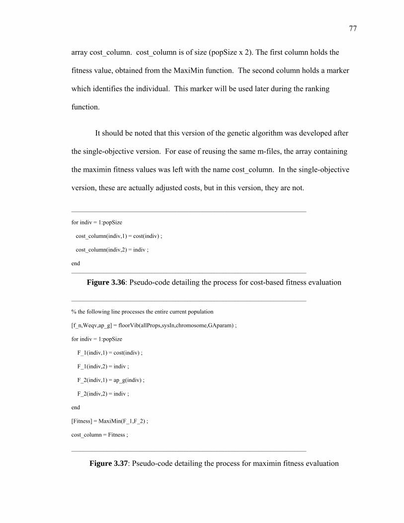
77
array cost_column. cost_column is of size (popSize x 2). The first column holds the
fitness value, obtained from the MaxiMin function. The second column holds a marker
which identifies the individual. This marker will be used later during the ranking
function.
It should be noted that this version of the genetic algorithm was developed after
the single-objective version. For ease of reusing the same m-files, the array containing
the maximin fitness values was left with the name cost_column. In the single-objective
version, these are actually adjusted costs, but in this version, they are not.
_______________________________________________________________________________
for indiv = 1:popSize
cost_column(indiv,1) = cost(indiv) ;
cost_column(indiv,2) = indiv ;
end _______________________________________________________________________________
Figure 3.36: Pseudo-code detailing the process for cost-based fitness evaluation
_______________________________________________________________________________
% the following line processes the entire current population
[f_n,Weqv,ap_g] = floorVib(allProps,sysIn,chromosome,GAparam) ;
for indiv = 1:popSize
F_1(indiv,1) = cost(indiv) ;
F_1(indiv,2) = indiv ;
F_2(indiv,1) = ap_g(indiv) ;
F_2(indiv,2) = indiv ;
end
[Fitness] = MaxiMin(F_1,F_2) ;
cost_column = Fitness ;
_______________________________________________________________________________
Figure 3.37: Pseudo-code detailing the process for maximin fitness evaluation
78
3.7 FUNCTION: floorVib.m
The function floorVib is used to evaluate the vibration performance of the steel floor
system represented by each individual. Values for floor system frequency, nf , total
effective weight of the floor system, W , and ratio of acceleration of the floor panel when
subjected to human walking with respect to the acceleration of gravity, pag
, are
calculated in this routine. A design procedure was followed that considered floor panel
acceleration due to walking excitation only. The procedure was contained in Chapter 4
of the AISC Steel Design Guide Series 11: Floor Vibrations Due to Human Activity
(AISC 1997).
In order to complete the vibration analysis, important problem data must first be
either chosen by the program user or obtained from established arrays. This data is
summarized in Figures 3.38 and 3.39. The value for ambient, or average, live load was
chosen as eleven pounds per square foot. This is a recommended value from the AISC
Series 11 Design Guide (AISC 1997), and was chosen to represent loading conditions
that would likely be present during building use. A more severe live loading was not
used because it is known that a heavier, more uniform load will not create the worst floor
system vibration problems. A superimposed dead loading of five pounds per square foot
is used within the function, representing the weight of floor covering, mechanical and
electrical systems, and suspended ceiling materials. The value for superimposed dead
loading is adjustable, and is stored within the function master in the array sysIn. The
value for the 28-day compressive strength of concrete, equal to 4,000 pounds per square
inch, was used for all calculations. This value is also adjustable within master in the

79
array sysIn. A calculation for the modulus of elasticity for the concrete, concE , is made
according to the equation 1.5( ) *conc conc cE density f= , where concdensity is in pcf and cf is
in ksi. Results for concE are in ksi. The given modulus of elasticity for the structural steel,
sE , was 29,000 ksi. The dynamic modular ratio, n , was computed using the equation
1.35*s
conc
EnE
= ,where sE and concE are of similar units. The dynamic modular ratio is
used to convert the concrete slab cross-section into an equivalent cross-section of steel,
making later calculation simpler.
The next step in vibration analysis involves the calculation of the beam mode
properties. Relevant pseudo-code is provided as Figure 3.39. The effective concrete slab
width is calculated as gLnBays
which must be less than 0.4 bL⋅ , where gL is the girder
length and bL is the beam length. Appropriate beam, slab, and deck properties are then
obtained for each individual from the array allProps which was created in
decodeChromo.
The location of the centroid of the composite cross section, y , with reference to
the top of the steel deck, is next computed using equation (3.5) ,
* * *
2 2
*
s r
s
d b aA h any bA a
n
⎛ ⎞ ⎛ ⎞+ −⎜ ⎟ ⎜ ⎟⎝ ⎠ ⎝ ⎠=
+ (3.5)
where sA is the cross-sectional area for the steel section, rh is the height of the steel deck
ribs, d is the depth for the steel section, b is the effective slab width, n is the dynamic

80
modular ratio, and a is the height of concrete above the ribs. y is calculated in inches
and a positive value indicates distance below the top of the steel deck.
The beam composite moment of inertia, jI , is computed next. The parallel-axis
theorem is used, as illustrated in equation (3.6),
2
1
n
j i i ii
I I A d=
= +∑ (3.6)
where n equals the number of parts (cross-section components) to be considered, iI
represents the moment of inertia for the ith part being considered, iA is the area for the ith
part, and id is the distance from the centroid of the ith part to the centroid of the entire
cross-section. For the composite cross-section being considered in this problem, this
equation is expanded as shown in equation (3.7),
2 23
2 12 2j s s rd b a b aI I A h y a y
n n⋅⎛ ⎞ ⎛ ⎞= + ⋅ + − + + ⋅ ⋅ +⎜ ⎟ ⎜ ⎟⋅⎝ ⎠ ⎝ ⎠
(3.7)
where all variables are defined with the commentary after equation (3.5). For each beam,
the uniformly distributed loading is calculated according to equation (3.8),
( )j conc deck beamw spacing LL DL wt wt wt= ⋅ + + + + (3.8)
where spacing is the beam spacing in feet, LL, DL, concwt , and deckwt are in pounds per
square feet, and beamwt is in pounds per linear foot. Results for the uniform loading are in
pounds per foot.
The corresponding beam deflection, jΔ , for each individual is given as equation
(3.9),

81
4
35*12
384j j
js j
w LE I
Δ = (3.9)
where jw is the load in pounds per foot, jL is the beam length in feet, sE is the modulus
of elasticity for steel in pounds per square inch, jI is the composite moment of inertia in
inches4, and 123 is a conversion factor for the conversion from feet3 to inches3. The beam
mode fundamental frequency, jf , is computed according to equation (3.10),
0.18jj
gf =Δ
(3.10)
where g is the acceleration of gravity in inches per second2 (386.4) and jΔ is the beam
deflection. Results for jf are in Hertz.
The average concrete thickness, ed , is next calculated according to 2
re
hd a= + ,
where rh is the rib height and a is the depth of concrete above the steel deck ribs. The
transformed moment of inertia per unit width in the slab span direction, sD , is calculated
according to equation (3.11),
312
12e
sdDn
= (3.11)
where ed is the average concrete thickness and n is the dynamic modular ratio. The result
for sD is in inches4/foot. The transformed moment of inertia per unit width in the beam
direction, jD , is calculated according to jj
ID
spacing= , where jI is in inches4 and
spacing is the beam spacing in feet to yield results with units of inches4 per foot. The
82
constant jC is selected next, as 2.0 for beams in areas including typical interior bays
(AISC 1997). The effective beam panel width, jB , is calculated next as shown in
equation (3.12),
14
sj j j
j
DB C LD
⎛ ⎞= ⎜ ⎟⎜ ⎟
⎝ ⎠ (3.12)
where , , ,j s jC D D and jL were defined earlier. The quantity, jB , must be less than or
equal to 23
⎛ ⎞⎜ ⎟⎝ ⎠
times the floor width, which for a typical interior bay would be equal to
three times the girder span, gL . The weight of the beam panel, jW , is calculated using
equation (3.13),
1.5 jj j j
wW B L
spacing⎛ ⎞
= ⎜ ⎟⎝ ⎠
(3.13)
where 1.5 is an adjustment factor included to account for continuity (AISC 1997), and
, ,j jw B and jL are described earlier in this section. Results for the beam panel weight are
in pounds.
Calculations for the girder mode properties are similar to those used for the beam
mode properties. Pseudo-code for the girder mode property calculations is provided in
Figure 3.40. The effective concrete slab width is calculated as 0.4 gL which must be less
than jL where gL is the girder length and jL is the beam length. The effective width is
then converted to inches for use in later calculations. Appropriate girder, slab, and deck
properties are then obtained for each individual from the array allProps which was
created in decodeChromo.

83
The location of the centroid of the composite cross section, y , with reference to
the top of the steel deck, is next computed according to equation (3.14),
* * *
2 2 2
*
ers e
s e
dh d bA dny bA d
n
⎛ ⎞⎛ ⎞+ −⎜ ⎟ ⎜ ⎟⎝ ⎠ ⎝ ⎠=
+ (3.14)
where sA is the cross-sectional area for the steel girder section, rh is the height of the
steel deck ribs, d is the depth for the steel section, b is the effective slab width, n is the
dynamic modular ratio, and ed is the average concrete thickness. y is calculated in
inches and a positive value indicates distance below the average concrete thickness ( ed ).
The girder composite moment of inertia, gI , is computed next. The parallel-axis
theorem is again used, as illustrated in equation (3.6). For the girder composite cross-
section being considered in this problem, equation (3.6) is expanded as shown below in
equation (3.15),
22
3* * *2 2 12 2
erg s s e e
dh d b bI I A y d d yn n
⎛ ⎞⎛ ⎞= + + − + + +⎜ ⎟ ⎜ ⎟⎝ ⎠ ⎝ ⎠
(3.15)
where sI is now the moment of inertia for the girder section and all other variables were
defined earlier.
For each girder, the equivalent uniform loading, gw , is calculated according to
equation (3.16),
jg j girder
ww L wt
spacing⎛ ⎞
= ⋅ +⎜ ⎟⎝ ⎠
(3.16)
84
where girderwt is the weight of the steel girder section in pounds per foot of length, and all
other values were described earlier. Results for the uniform loading are in pounds per
foot. The corresponding girder deflection, gΔ , is computed using equation (3.17),
4
35*12
384g g
gs g
w LE I
Δ = (3.17)
where gw is the load in pounds per foot, gL is the girder length in feet, sE is the modulus
of elasticity for steel in pounds per square inch, gI is the composite moment of inertia in
inches4, and 123 is a conversion factor for going from feet3 to inches3. The girder mode
fundamental frequency, gf , is computed according to equation (3.18),
0.18gg
gf =Δ
(3.18)
where g is the acceleration of gravity in inches per second2 (386.4) and gΔ is the girder
deflection. Results for gf are in Hertz. The flexural rigidity of the girder per unit
width, gD , is calculated next according to equation (3.19),
gg
j
ID
L= (3.19)
where gI is the girder composite moment of inertia and jL is the length of the beam in
feet. Results for gD have units of inches4 per foot.
The value gC , the girder panel width modification factor, is chosen next. gC is
equal to 1.6 for girders supporting joists or beams connected to the girder flange and is

85
equal to 1.8 for girders supporting beams connected to the girder web. For the two
versions of the genetic algorithm presented in this thesis, gC will always be equal to 1.8.
The effective girder panel width, gB , is calculated as shown in equation (3.20),
14
jg g g
g
DB C L
D⎛ ⎞
= ⎜ ⎟⎜ ⎟⎝ ⎠
(3.20)
where all variables have been defined previously. The quantity, gB , must be less than or
equal to 23
⎛ ⎞⎜ ⎟⎝ ⎠
times the floor length, which for a typical interior bay would be equal to
three times the beam span, jL . The weight of the girder panel, gW , is calculated using
equation (3.21),
gg g g
j
wW B L
L= (3.21)
where all variables have been defined earlier. The value for gW was not increased by
50%, as jW was, because continuity effects are generally not realized when girders frame
directly into columns. Results for the girder panel weight are in pounds. If the girder
span, gL , is less than the joist panel width, jB , then the girder deflection is reduced
according to equation (3.22),
gg g
j
LB
′Δ = Δ (3.22)
where all variables have been defined earlier in this section.
The third section of the function floorVib is used to calculate the three vibration
parameters of the floor system which are floor fundamental frequency, nf , equivalent

86
panel mode weight, W, and floor panel acceleration with respect to gravity, pag
. Pseudo-
code for this section of the function floorVib can be viewed in Figure 3.41. The floor
fundamental frequency, nf , is calculated according to equation (3.23),
0.18nj g
gf =Δ + Δ
(3.23)
where g is the acceleration of gravity in inches per second2 (386.4) and jΔ and gΔ are
the beam deflection and the girder deflection, respectively. Results for nf are in Hertz.
The equivalent panel weight, W, is calculated using equation (3.24),
j gj g
j g j g
W W WΔ Δ
= +Δ + Δ Δ + Δ
(3.24)
where all variables have been defined previously. Results for the equivalent panel weight
are in pounds.
The dimensionless acceleration value, pag
, is computed according to the method
presented by Murray et al. (1997),
( 0.35 )
100%nf
p oa P eg Wβ
−
= ⋅ (3.25)
where oP is a constant force in pounds, usually 65 pounds, nf and W were described
earlier, and β is a damping ratio. For offices and residences, the recommended range for
β is 0.02 to 0.05. The value used in the runs made for this thesis was 0.03.
Recommended acceptable acceleration limits for offices and residences are usually given
as 0.5%.
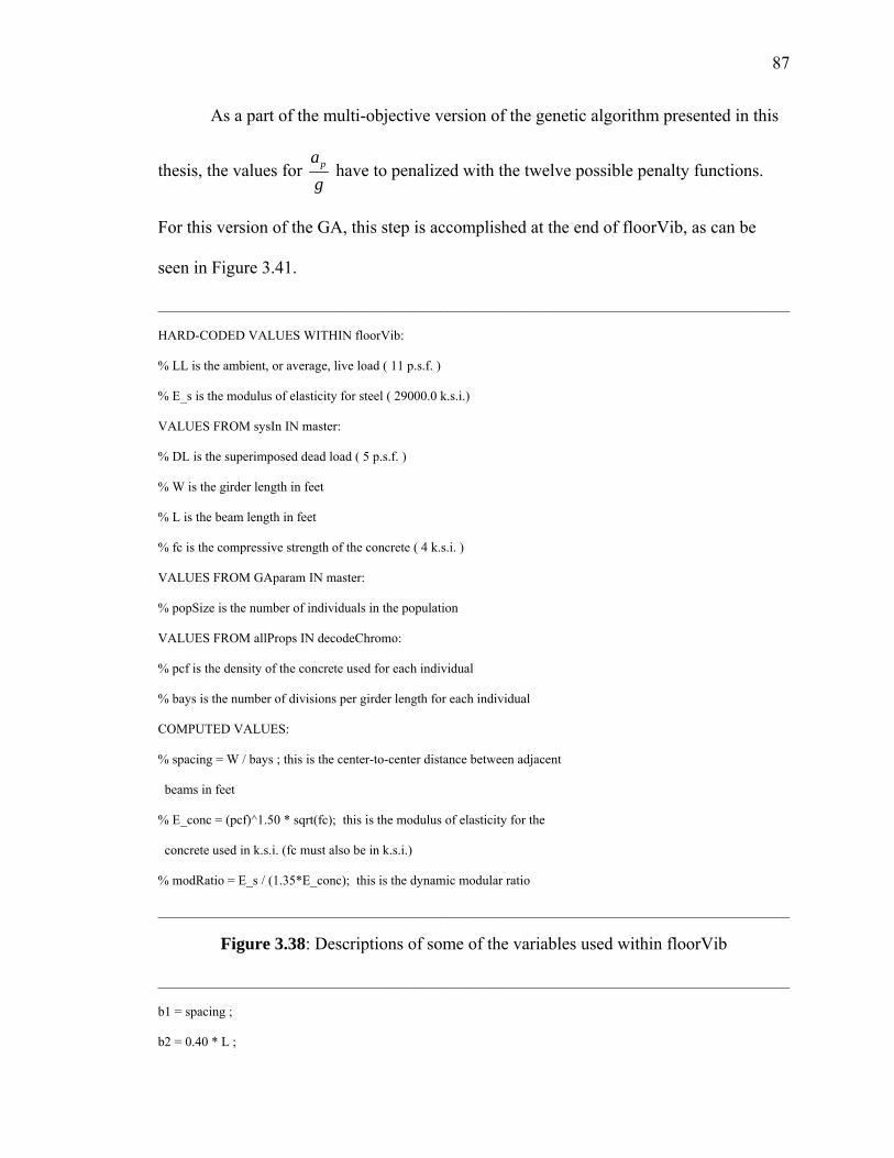
87
As a part of the multi-objective version of the genetic algorithm presented in this
thesis, the values for pag
have to penalized with the twelve possible penalty functions.
For this version of the GA, this step is accomplished at the end of floorVib, as can be
seen in Figure 3.41.
________________________________________________________________________________________________
HARD-CODED VALUES WITHIN floorVib:
% LL is the ambient, or average, live load ( 11 p.s.f. )
% E_s is the modulus of elasticity for steel ( 29000.0 k.s.i.)
VALUES FROM sysIn IN master:
% DL is the superimposed dead load ( 5 p.s.f. )
% W is the girder length in feet
% L is the beam length in feet
% fc is the compressive strength of the concrete ( 4 k.s.i. )
VALUES FROM GAparam IN master:
% popSize is the number of individuals in the population
VALUES FROM allProps IN decodeChromo:
% pcf is the density of the concrete used for each individual
% bays is the number of divisions per girder length for each individual
COMPUTED VALUES:
% spacing = W / bays ; this is the center-to-center distance between adjacent
beams in feet
% E_conc = (pcf)^1.50 * sqrt(fc); this is the modulus of elasticity for the
concrete used in k.s.i. (fc must also be in k.s.i.)
% modRatio = E_s / (1.35*E_conc); this is the dynamic modular ratio
________________________________________________________________________________________________
Figure 3.38: Descriptions of some of the variables used within floorVib
________________________________________________________________________________________________
b1 = spacing ;
b2 = 0.40 * L ;

88
b = 12.0*min(b1,b2) ;
VALUES FROM allProps IN decodeChromo:
% A_s is the beam cross-sectional area (in inches ^ 2)
% I_s is the beam moment of inertia (in inches ^ 4)
% h_r is the height of the steel deck rib (in inches)
% d is the depth of the beam section (in inches)
% a is the height of concrete above the steel deck rib (in inches)
% conc is the weight of the concrete is p.s.f.
% deck is the weight of the deck in p.s.f.
% beam is the weight of the beam in p.l.f.
yBar = (A_s*(h_r + d/2) - (b/modRatio)*a*(a/2)) / (A_s + b/modRatio*a) ;
I_j = I_s + A_s*(h_r + d/2 - yBar)^2 + (b/modRatio)*(a^3)/12.0 ...
+ (b/modRatio)*a*(yBar + a/2)^2;
w_j = spacing*(LL + DL + conc + deck) + beam ;
Delta_j = (5.0*w_j*L^4) / (384.0*E_s*I_j)*1728.0 ;
f_j = 0.18*sqrt (386.4 / Delta_j);
d_e = h_r/2.0 + a ;
A = 12.0*d_e/modRatio;
D_s = (12.0/modRatio)*(d_e^3/12.0) ;
D_j = I_j / spacing ;
C_j = 2.0;
B1 = (2.0/3.0) * W * 3 ;
B2 = C_j*(D_s/D_j)^0.25 * L ;
B_j = min(B1,B2);
W_j = 1.5*(w_j/spacing)*B_j * L ;
________________________________________________________________________________________________
Figure 3.39: Pseudo-code used for calculation of beam mode properties
________________________________________________________________________________________________
b1 = 0.40 * W ;
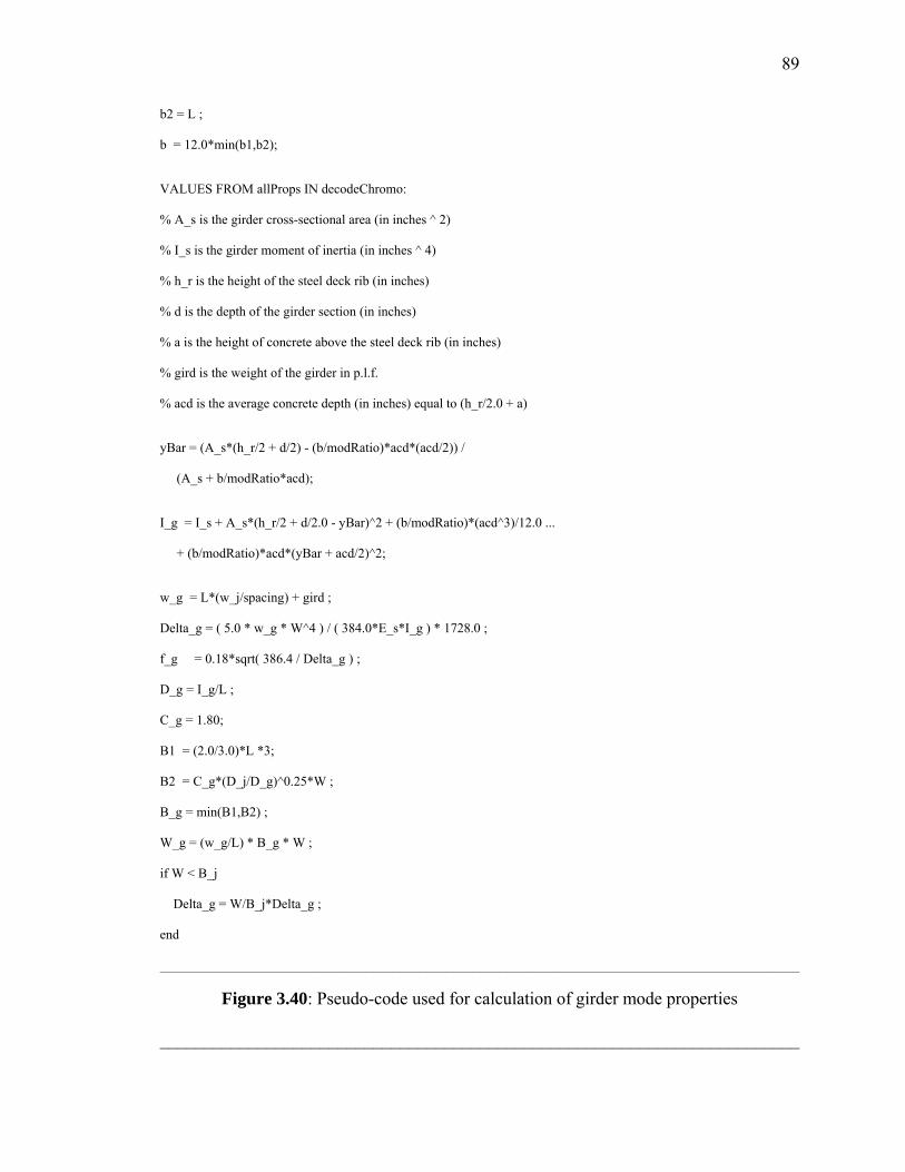
89
b2 = L ;
b = 12.0*min(b1,b2);
VALUES FROM allProps IN decodeChromo:
% A_s is the girder cross-sectional area (in inches ^ 2)
% I_s is the girder moment of inertia (in inches ^ 4)
% h_r is the height of the steel deck rib (in inches)
% d is the depth of the girder section (in inches)
% a is the height of concrete above the steel deck rib (in inches)
% gird is the weight of the girder in p.l.f.
% acd is the average concrete depth (in inches) equal to (h_r/2.0 + a)
yBar = (A_s*(h_r/2 + d/2) - (b/modRatio)*acd*(acd/2)) /
(A_s + b/modRatio*acd);
I_g = I_s + A_s*(h_r/2 + d/2.0 - yBar)^2 + (b/modRatio)*(acd^3)/12.0 ...
+ (b/modRatio)*acd*(yBar + acd/2)^2;
w_g = L*(w_j/spacing) + gird ;
Delta_g = ( 5.0 * w_g * W^4 ) / ( 384.0*E_s*I_g ) * 1728.0 ;
f_g = 0.18*sqrt( 386.4 / Delta_g ) ;
D_g = I_g/L ;
C_g = 1.80;
B1 = (2.0/3.0)*L *3;
B2 = C_g*(D_j/D_g)^0.25*W ;
B_g = min(B1,B2) ;
W_g = (w_g/L) * B_g * W ;
if W < B_j
Delta_g = W/B_j*Delta_g ;
end
________________________________________________________________________________________________
Figure 3.40: Pseudo-code used for calculation of girder mode properties
________________________________________________________________________
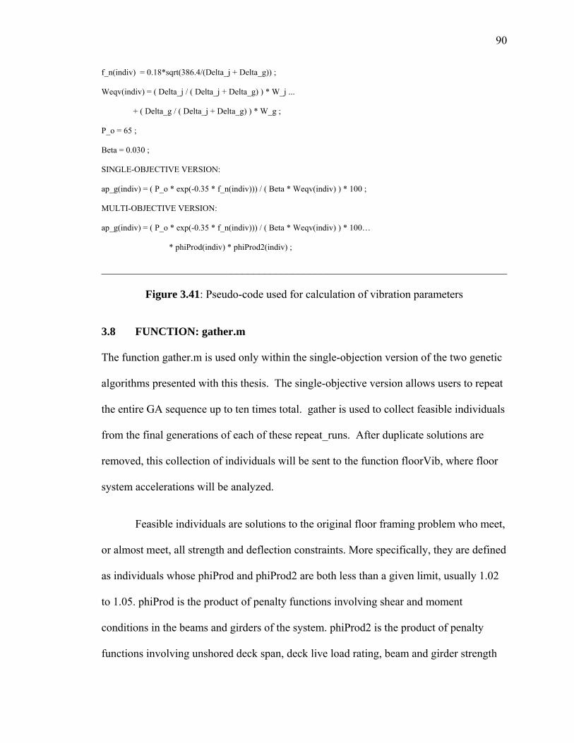
90
f_n(indiv) = 0.18*sqrt(386.4/(Delta_j + Delta_g)) ;
Weqv(indiv) = ( Delta_j / ( Delta_j + Delta_g) ) * W_j ...
+ ( Delta_g / ( Delta_j + Delta_g) ) * W_g ;
P_o = 65 ;
Beta = 0.030 ;
SINGLE-OBJECTIVE VERSION:
ap_g(indiv) = ( P_o * exp(-0.35 * f_n(indiv))) / ( Beta * Weqv(indiv) ) * 100 ;
MULTI-OBJECTIVE VERSION:
ap_g(indiv) = ( P_o * exp(-0.35 * f_n(indiv))) / ( Beta * Weqv(indiv) ) * 100…
* phiProd(indiv) * phiProd2(indiv) ;
________________________________________________________________________
Figure 3.41: Pseudo-code used for calculation of vibration parameters
3.8 FUNCTION: gather.m
The function gather.m is used only within the single-objection version of the two genetic
algorithms presented with this thesis. The single-objective version allows users to repeat
the entire GA sequence up to ten times total. gather is used to collect feasible individuals
from the final generations of each of these repeat_runs. After duplicate solutions are
removed, this collection of individuals will be sent to the function floorVib, where floor
system accelerations will be analyzed.
Feasible individuals are solutions to the original floor framing problem who meet,
or almost meet, all strength and deflection constraints. More specifically, they are defined
as individuals whose phiProd and phiProd2 are both less than a given limit, usually 1.02
to 1.05. phiProd is the product of penalty functions involving shear and moment
conditions in the beams and girders of the system. phiProd2 is the product of penalty
functions involving unshored deck span, deck live load rating, beam and girder strength
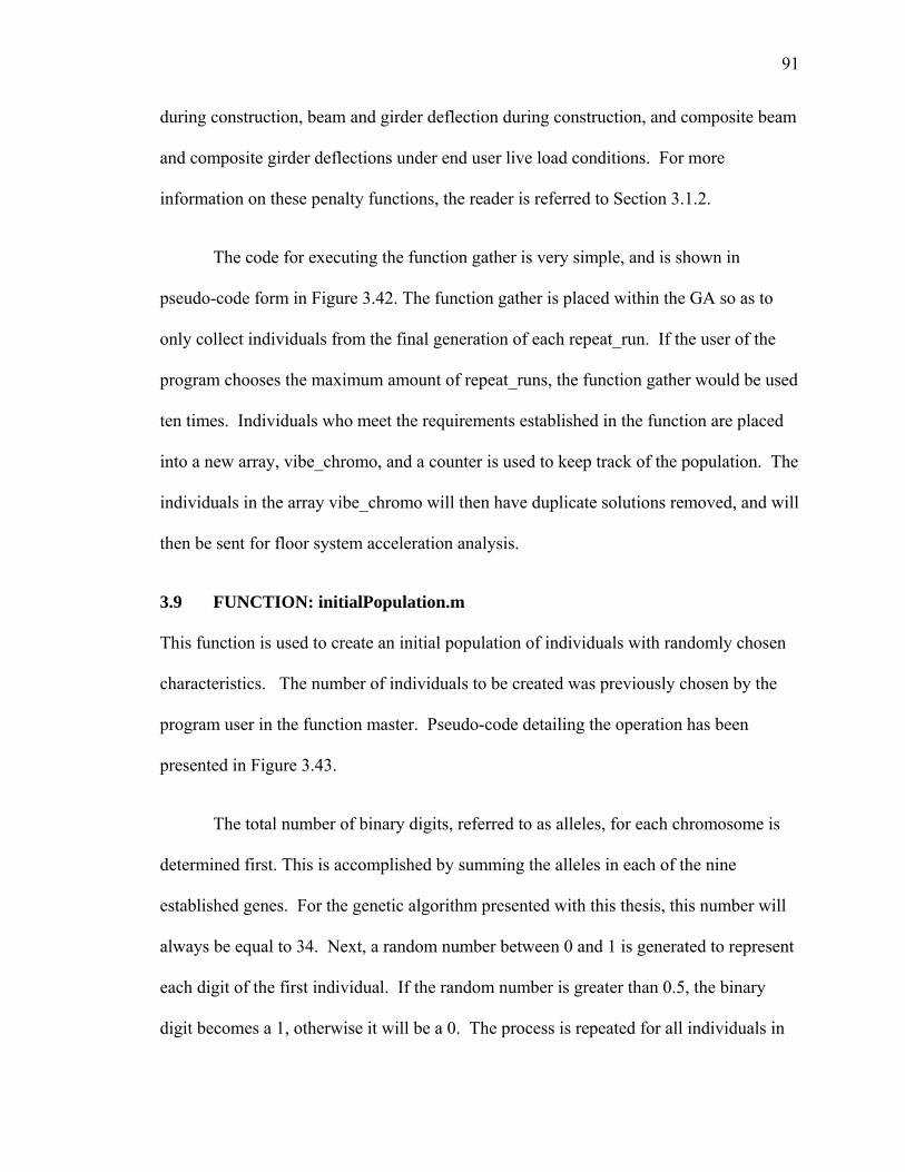
91
during construction, beam and girder deflection during construction, and composite beam
and composite girder deflections under end user live load conditions. For more
information on these penalty functions, the reader is referred to Section 3.1.2.
The code for executing the function gather is very simple, and is shown in
pseudo-code form in Figure 3.42. The function gather is placed within the GA so as to
only collect individuals from the final generation of each repeat_run. If the user of the
program chooses the maximum amount of repeat_runs, the function gather would be used
ten times. Individuals who meet the requirements established in the function are placed
into a new array, vibe_chromo, and a counter is used to keep track of the population. The
individuals in the array vibe_chromo will then have duplicate solutions removed, and will
then be sent for floor system acceleration analysis.
3.9 FUNCTION: initialPopulation.m
This function is used to create an initial population of individuals with randomly chosen
characteristics. The number of individuals to be created was previously chosen by the
program user in the function master. Pseudo-code detailing the operation has been
presented in Figure 3.43.
The total number of binary digits, referred to as alleles, for each chromosome is
determined first. This is accomplished by summing the alleles in each of the nine
established genes. For the genetic algorithm presented with this thesis, this number will
always be equal to 34. Next, a random number between 0 and 1 is generated to represent
each digit of the first individual. If the random number is greater than 0.5, the binary
digit becomes a 1, otherwise it will be a 0. The process is repeated for all individuals in
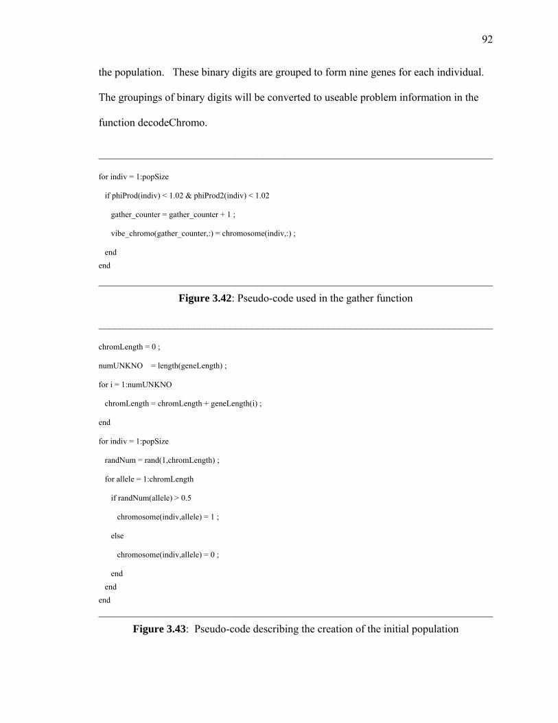
92
the population. These binary digits are grouped to form nine genes for each individual.
The groupings of binary digits will be converted to useable problem information in the
function decodeChromo.
________________________________________________________________________
for indiv = 1:popSize
if phiProd(indiv) < 1.02 & phiProd2(indiv) < 1.02
gather_counter = gather_counter + 1 ;
vibe_chromo(gather_counter,:) = chromosome(indiv,:) ;
end end
________________________________________________________________________ Figure 3.42: Pseudo-code used in the gather function
________________________________________________________________________
chromLength = 0 ;
numUNKNO = length(geneLength) ;
for i = 1:numUNKNO
chromLength = chromLength + geneLength(i) ;
end
for indiv = 1:popSize
randNum = rand(1,chromLength) ;
for allele = 1:chromLength
if randNum(allele) > 0.5
chromosome(indiv,allele) = 1 ;
else
chromosome(indiv,allele) = 0 ;
end end end ________________________________________________________________________
Figure 3.43: Pseudo-code describing the creation of the initial population
93
3.10 FUNCTION: master.m
The use of a graphical user interface (GUI) for the program was discussed, but rejected
due to time constraints. Instead, all of the user input is included within a single function
titled master. The user input is contained in four arrays. They are titled sysIn, costIn,
geneLength, and GAparam. The four arrays can be seen in the full listing of MATLAB
code which has been included as Appendix A.11.
The array sysIn contains all of the data that describes the structural engineering
problem. (A more complete description of the problem data can be seen Section 1.3.)
sysIn = [W,L,q,comp,desGen,Fy,fc,studDia,fu,studUp]
The variable W is the width of the panel, and will be the girder length. L is the length of
the panel, and will be the beam length. q is an array where q(1) and q(2) are the
superimposed dead load and live load, respectively. comp is assigned to indicate whether
composite action will be permitted, with a 1 meaning yes and a 2 meaning no, but this
marker is not currently being used within the genetic algorithm. desGen indicates the
total number of generations that should be completed within the genetic algorithm. Fy
indicates the yield strength of the steel sections in kips per square inch. Fc indicates the
28-day compressive strength of the concrete to be used in the slab in pounds per square
inch. studDia indicates the diameter to be used for the shear studs, usually 0.75-inches.
Fu indicates the tensile strength for the shear studs in kips per square inch. The last input
studUp indicates how far above the deck ribs the shear studs will extend. This last input
is usually 1.5-inches.
The array costIn contains the user’s most accurate cost information regarding
material, fabrication, and erection costs. These numbers are used later in the genetic
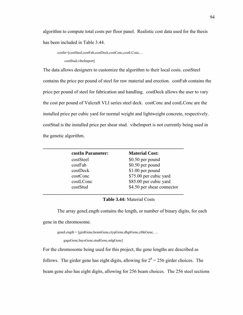
94
algorithm to compute total costs per floor panel. Realistic cost data used for the thesis
has been included in Table 3.44.
costIn=[costSteel,costFab,costDeck,costConc,costLConc,…
costStud,vibeImport]
The data allows designers to customize the algorithm to their local costs. costSteel
contains the price per pound of steel for raw material and erection. costFab contains the
price per pound of steel for fabrication and handling. costDeck allows the user to vary
the cost per pound of Vulcraft VLI series steel deck. costConc and costLConc are the
installed price per cubic yard for normal weight and lightweight concrete, respectively.
costStud is the installed price per shear stud. vibeImport is not currently being used in
the genetic algorithm.
___________________________________________________________
costIn Parameter: Material Cost:
costSteel $0.50 per pound costFab $0.50 per pound costDeck $1.00 per pound costConc $75.00 per cubic yard costLConc $85.00 per cubic yard costStud $4.50 per shear connector
___________________________________________________________ Table 3.44: Material Costs
The array geneLength contains the length, or number of binary digits, for each
gene in the chromosome.
geneLength = [girdGene,beamGene,ctypGene,dhgtGene,cthkGene, …
gageGene,baysGene,studGene,stdgGene]
For the chromosome being used for this project, the gene lengths are described as
follows. The girder gene has eight digits, allowing for 28 = 256 girder choices. The
beam gene also has eight digits, allowing for 256 beam choices. The 256 steel sections
95
available as beam and girder choices are identical, and are taken from the AISC Manual
(AISC 2001).
The concrete-type gene has only one digit, allowing for 21 = 2 choices. These
choices are simply normal-weight and light-weight concrete mixes. The deck-height gene
also has only one digit, again allowing for two choices. These choices are for 1.5-inch
and 3.0-inch rib heights.
The concrete-thickness gene has two digits, allowing 22 = 4 choices. These
thicknesses vary, depending on the concrete type. The deck gage gene has two digits,
with the four choices being 19, 20, 21, and 22-gage. The bays gene also has two digits,
with the four choices being two, three, four, or five divisions per panel width. As an
example, a choice of three would mean the girder length would be divided into three
zones by the beams that frame into it. The beam-stud gene and the girder-stud gene each
have five digits, allowing 25 = 32 choices. These choices vary from zero to 124 studs per
half span, in multiples of four.
The array GAparam contains the variables that control the operation of the genetic
algorithm.
GAparam = [maxGen,cp,mp,par,ef,pop]
The variable maxGen was designed to control the number of generations for each GA
run, but the variable desGen in the array sysIn is being used instead. cp controls the
operation of the population partitioning scheme, that is used as the basis for the selection
mechanism. The variable cp indicates the location of the cut-off for the 75% / 25%
partitioning method, with commonly used values ranging from 30 to 40 %. A description
96
of this selection method is included in Section 3.15. mp is the mutation probability,
usually 0.015 to 0.025 (1.5 to 2.5 %). par defines the parental carry-over to the next
generation. As an example, 100 % carry-over means that 50% of the most-fit parents will
comprise 50% of the next generation. ef signals whether or not elitism will be used.
Elitism must be on to allow the parental carry-over described previously. Elitism also
protects the most-fit individual in the previous generation from mutation. pop is the size
of the population to be used in the GA. Populations usually range from 200 to 400.
Following the initialization of the four user input arrays, the function executeGA
is utilized. The function executeGA will serve to control the sequencing of the other m-
files that make up the genetic algorithm.
An attempt has been made to include all of the user input within the single
function, master.m. However, there are a few exceptions, which will be listed in this
section for any future users of the program.
1. There are various deflection limits hard-coded within the function moreChecks.
The reader is referred to Appendix A.13 for the full listing of program code used
for this function.
2. If running the program in its single-objective form, there is a variable repeat_runs
in the top of the file executeGA, which controls the number of times the entire
GA is repeated. The reader is referred to Appendix A.5 for the full listing of
program code used in this function.
3.11 FUNCTION: maximin.m
The maximin function is used only within the multi-objective version of the genetic
algorithm presented with this thesis. The maximin fitness function was developed by

97
Richard Balling and Scott Wilson (Balling, et al 2001). It provides a method for the
evaluation of each individual solution based on both total adjusted panel cost and non-
dimensional floor panel acceleration. In contrast, the single-objective version of the GA
uses only total adjusted panel cost in the definition of an individual’s fitness.
The Maximin fitness method is a Pareto-based approach to multi-objective fitness
optimization. Pareto-based approaches are well-established (Goldberg 1989). The
Pareto-front is defined as the collection of all non-dominated designs for a given
problem. A solution is considered to be dominated “…if there exists another design in
the population that is better or equal in every objective, and better in at least one
objective” (Balling, et al 2001). A plot that illustrates the general shape of the Pareto
front has been included as Figure 3.45.
The maximin fitness function “…directs genetic algorithms toward final
generations that are both close to the universal Pareto front and diverse” (Balling, et al
2001). The pseudo-code used to compute the maximin fitness is included as Figure 3.46.
The Maximin fitness function has several advantages over other Pareto-based
approaches. It can easily be generalized to work with any number of objectives. The
Maximin fitness function is designed to provide equal preference to the multiple
objectives and it is relatively simple to program. Most importantly, it has the ability to
prevent clustering of solutions within areas of the Pareto front. The maximin fitness
function encourages spreading of the solutions along the front, thus enabling final
decisions with respect to trade-offs among objectives to be made, based on well-defined
choices.
98
The Maximin fitness function does have a few disadvantages. It requires that a
large number of comparisons be made for each generation. Each solution is compared
with all other solutions within the generation, and this can require large amounts of time
to process if populations are large. Also, because of the way in which comparisons are
made, the maximin fitness function requires that duplicate solutions be removed from the
population, or that provisions be made to avoid comparisons of identical solutions.
The maximin fitness for an individual within the context of a two-objective
problem is given by,
( ){ }1 2 21.0 max min ,i i ij i jj iF f f f f
≠= − − − (3.26)
where iF is the maximin fitness for individual i, 1if and 1 jf are Objective 1 magnitudes
for individuals i and j, respectively, and 2if and 2 jf are the Objective 2 magnitudes for
individuals i and j, respectively. The first objective for the problem presented in this
document is,
11
constrN
ii
f cost=
= ⋅ Φ∏ (3.27)
where cost is the total floor panel cost, constrN is the total number of problem constraints
included in the fitness statement, and iΦ are the penalty functions associated with the
given constraints. The second objective for the problem presented in this document is,
21
constrNp
ii
af
g =
= ⋅ Φ∏ (3.28)
99
where pag
is the floor panel acceleration due to walking excitation with respect to the
acceleration of gravity, constrN is the total number of problem constraints included in the
fitness statement, and iΦ are the penalty functions associated with the given constraints
discussed previously.
A series of six MATLAB plots are presented in Figure 3.47, illustrating progress
of the Maximin fitness function within one complete run of the genetic algorithm. The
plots show the cost and acceleration values for the top 100 individuals in a 200 individual
population after the first, fifth, tenth, twentieth, thirtieth, and fortieth generations. It can
be seen that the solutions begin to move toward a shape like that of a convex Pareto front.
It can be seen that diversity is encouraged as individuals initially move toward both low
cost and low acceleration regions. There is a nearly uniform distribution of individuals
along the front exhibited in the plots.
After the fortieth generation, it can be seen that the low acceleration region of the
solution space is favored. This behavior represents a problem, as very strong, very
expensive solutions are not desired as practical solutions to the problem considered in
this thesis. Equal weight is being placed on each of the two objectives, and it is easier for
the GA to find solutions that fit the low-acceleration region, as compared to those
solutions which are very low-cost with high-acceleration.
When the GA is evaluating randomly-generated solutions, all that must happen to
create a high-cost, low-acceleration individual is the selection of a very large beam
section and a very large girder section. The list of available sections for beams and

100
girders includes beam sections w44x335, w40x593, w35x848, w33x354, w30x477, and
w27x539; and the column sections w14x808 and w12x336. It is very likely that a large
section might be selected. The choice of very large beam and girder sections will meet
all strength and deflection constraints, and have no penalty functions applied. The
solution is treated by the maximin fitness evaluator as a very good solution, despite the
very high cost, and is allowed to proliferate within the population.
In contrast, the creation of a very low-cost, high-acceleration individual is much
more difficult. The list of available sections for beams and girders includes sections as
small as w8x13, w10x12, w12x14, and w14x22. These sections might often be selected
as beam and girder sections, but will quickly be eliminated as penalty factors accumulate
because of deficient strength and deflection capacities. To create a single low-cost, high-
acceleration individual, the GA often will cycle through many generations, and combine
properties from many different individuals.
The implementation of the maximin fitness evaluator within the multi-objective
genetic algorithm was successful. It did direct the genetic algorithm toward final
generations that were both close to the Pareto front and diverse. However, the maximin
fitness function is not effective within the context of this floor framing problem for two
reasons. First, it does not distinguish between the importance of the two objectives. It
treats both equally, with no understanding or interpretation of individual results. Second,
the Maximin fitness function does not recognize the relative ease and difficulty with
which high-cost, low-acceleration and low-cost, high-acceleration individuals are
produced.
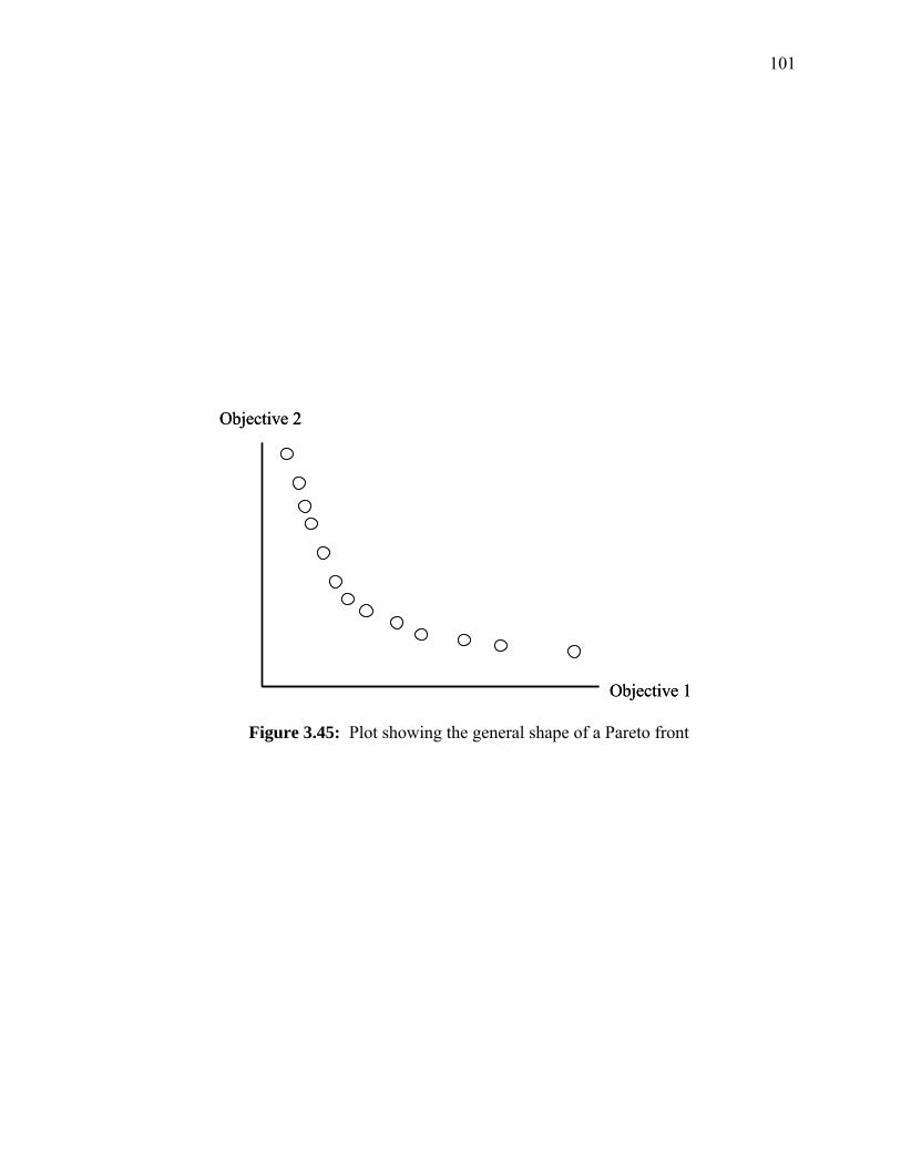
101
Objective 2
Objective 1
Objective 2
Objective 1
Figure 3.45: Plot showing the general shape of a Pareto front
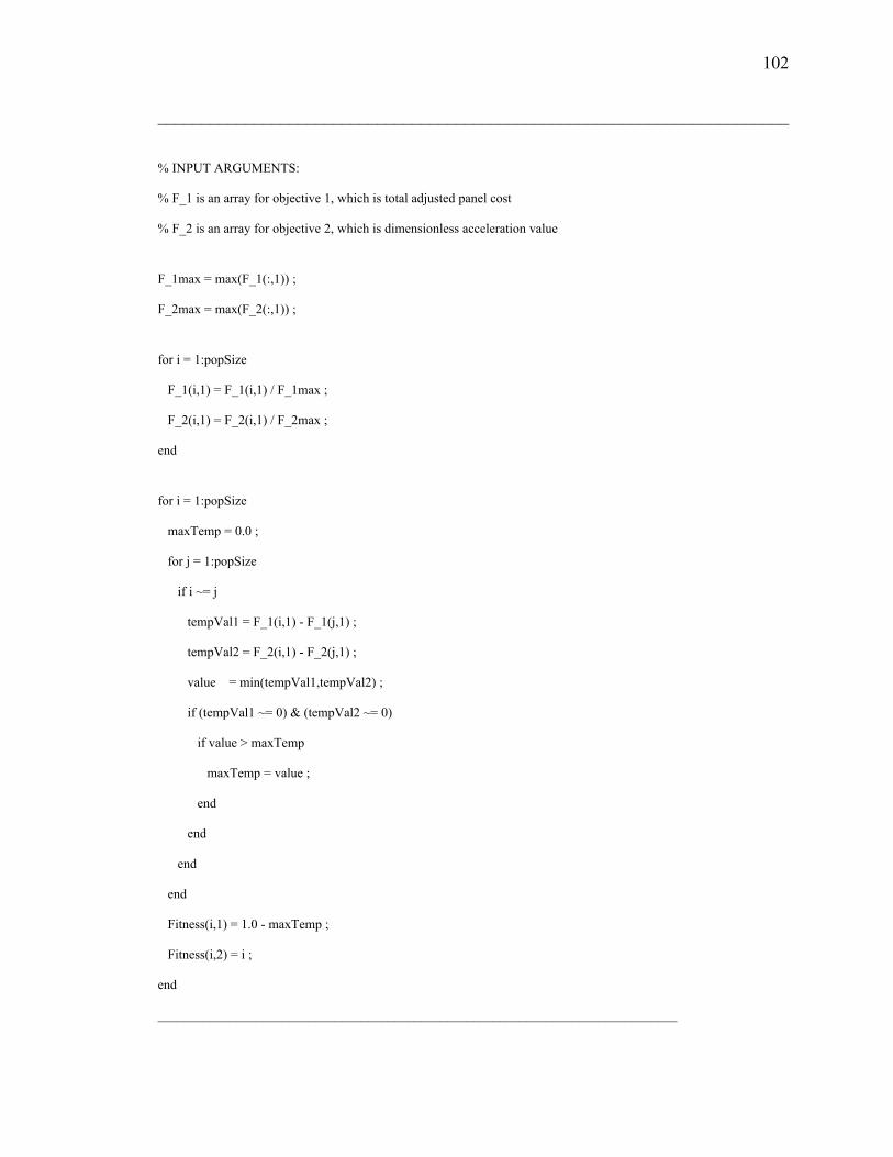
102
________________________________________________________________________
% INPUT ARGUMENTS:
% F_1 is an array for objective 1, which is total adjusted panel cost
% F_2 is an array for objective 2, which is dimensionless acceleration value
F_1max = max(F_1(:,1)) ;
F_2max = max(F_2(:,1)) ;
for i = 1:popSize
F_1(i,1) = F_1(i,1) / F_1max ;
F_2(i,1) = F_2(i,1) / F_2max ;
end
for i = 1:popSize
maxTemp = 0.0 ;
for j = 1:popSize
if i ~= j
tempVal1 = F_1(i,1) - F_1(j,1) ;
tempVal2 = F_2(i,1) - F_2(j,1) ;
value = min(tempVal1,tempVal2) ;
if (tempVal1 ~= 0) & (tempVal2 ~= 0)
if value > maxTemp
maxTemp = value ;
end
end
end
end
Fitness(i,1) = 1.0 - maxTemp ;
Fitness(i,2) = i ;
end
_______________________________________________________________________________
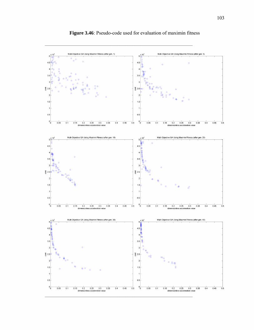
103
Figure 3.46: Pseudo-code used for evaluation of maximin fitness
_______________________________________________________________________________
_______________________________________________________________________________
104
Figure 3.47: MATLAB plots demonstrating progress of maximin fitness function
3.12 FUNCTION: moreCheck.m
moreCheck.m is the second of two sub-functions called under the m-file allChecks.m.
moreCheck.m evaluates additional violations relating to deck, beam, and girder strength,
deflection, and performance. The first two checks in moreCheck.m are used to verify
beam and girder bending capacity during construction. The next two checks are for
deflection of the composite beam and deflection of the composite girder under live load
conditions. The following two checks are used to verify beam and girder deflections
during construction. Checks are next made for deck unshored clear span distance and
deck live load rating. An optional check, for floor panel acceleration, is used only within
the third version of the genetic algorithm presented with this thesis. This version uses a
single-objective fitness statement, but includes floor panel acceleration due to walking
excitation as a penalty function.
These checks, along with the first four made within vmCheck.m, are used in
conjunction with a penalized objective function. This penalized objective function is
described in more detail in Section 3.1.2. The design checks are explained with
additional detail in Chapter 4.
3.13 FUNCTION: mutation.m
Mutation is introduced within the genetic algorithm reproductive sequence in an attempt
to guide the GA into exploring new areas of the search space. The use of the mutation
operator can introduce new traits into the population and prevent the GA from
converging too fast to a local minimum (Haupt, et al 1998).
105
Single-point mutations are being used by the authors in this thesis project. A
mutation rate is established as a part of the array GAparam in the m-file master. The
mutation rate is typically 1.5% to 2.5% of digits per generation. Increasing this rate
allows the GA more freedom to explore new areas of the solution space. Too high of a
mutation rate, though, can also distract the GA from converging. Conversely, too low of
a mutation rate can lead the GA to converge on local minima which may not represent
good solutions to the problem (Haupt, et al 1998).
According to the established mutation probability, individual digits in the parent
chromosomes of each generation are subject to mutation. (The reader should note that
mutation does not occur within the initial generation.) If a digit is selected for mutation,
its value is switched to 1 if it was 0, or to 0 if it was 1. The steps in executing the
mutation operation will be summarized. Pseudo-code illustrating the mutation procedure
is included in Figure 3.48.
According to the variable definitions,
popSize = number of individuals within the population, typically 200 to 300
chromLength = number of digits with the chromosome of each individual, equal to 34
an array of size ( popSize x chromLength ) is filled with random numbers ranging from 0
to 1. The random numbers are created using MATLAB’s random number generator. The
random number representing each digit of every chromosome is compared against the
mutation rate, and switched if it falls below the rate. For this part of the function, the
mutation rate is expressed as a decimal form, with 0.015 representing 1.5%.
As a part of the elitism scheme that was established within the m-file selection,
the most-fit individual that was allowed to pass freely from the previous generation is
106
given special treatment. This individual was allowed to pass freely as part of a group of
size par, which was established in the function master. In order for this movement to
happen, the elitism flag within the array GAparam in the m-file master must be in the on
position.
The special treatment for this most-fit individual protects its chromosome from
the mutation operator. This was done to ensure that the genetic material contained within
this most-fit individual is not lost. In order to provide this protection within the mutation
function, the random numbers representing the digits of this most-fit individual are first
located and then altered to a given value, 0.7500. The value 0.7500 is arbitrary, it must
only be greater than the mutation probability. This step ensures that the random number
representing each digit is greater than the mutation probability limit, and so no digits will
be changed.
3.14 FUNCTION: ranking.m
Ranking is a function used within the genetic algorithm sequence to reorder the
population of chromosomes from most-fit to least-fit.
As two versions of the GA are presented with this project, two forms of fitness are
used. In the single-objective genetic algorithm, fitness is simply defined as the total cost
per framing panel multiplied by the product of all penalty factors (total adjusted panel
cost). In the multiple-objective version, fitness is determined by the Maximin fitness
function (Balling, et al 2001). The Maximin fitness is calculated using both total
adjusted panel cost and floor system acceleration information.
________________________________________________________________________

107
% popSize = number of individuals within the population, typically 200 to 300
% chromLength = number of digits with the chromosome of each individual, equal to 34
% random_mutation = an array of size ( popSize x chromLength ) filled with random
numbers between 0 and 1.
% chromosome = an array of size ( popSize x chromLength ) which contains the digits
that represent the genetic material of each individual
% mutation_prob = mutation probability in decimal form (0.015 represents 1.5%)
for indiv = 1:popSize
for digit = 1:chromLength
if random_mutation(indiv,digit) < mutation_prob
if chromosome(indiv,digit) == 0
chromosome(indiv,digit) = 1 ;
else
chromosome(indiv,digit) = 0 ;
end
end
end
end
________________________________________________________________________
Figure 3.48: Pseudo-code illustrating the mutation procedure
The ranking function receives a ( population_size x 2 ) array containing fitness
and individual identifier information of the form shown in Figure 3.49.
Fitness Identifier 2500 1 4580 2 1355 3 2295 4 3585 5
Figure 3.49: Fitness array for ranking function

108
The next operation is to sort the array, based on fitness, and still carry the individual
identifier along with each fitness value. This is performed with a simple column sort
routine, which was developed by the author. Pseudo-code for this routine is shown in
Figure 3.50.
________________________________________________________________________
for i = 1:popSize
for j = 1:(popSize - 1)
if cost_column(j+1, 1) > cost_column(j, 1)
for k = 1:2
temp(k) = cost_column(j,k);
cost_column(j,k) = cost_column(j+1,k);
cost_column(j+1,k) = temp(k);
end
end
end
end
_______________________________________________________________________
Figure 3.50: Pseudo-code used for the column sort procedure
The routine begins in the fitness column and compares the first two fitness values.
If the first is better (could be greater or less than depending on GA version), then nothing
happens. But, it the second is better, the two values are switched. This single
comparison step proceeds down the column. When the end of the column has been
reached, the routine has served to transfer the single least-fit value to the very bottom.
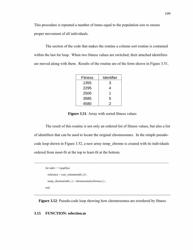
109
Fitness Identifier 1355 3 2295 4 2500 1 3585 5 4580 2
This procedure is repeated a number of times equal to the population size to ensure
proper movement of all individuals.
The section of the code that makes the routine a column sort routine is contained
within the last for loop. When two fitness values are switched, their attached identifiers
are moved along with them. Results of the routine are of the form shown in Figure 3.51.
Figure 3.51: Array with sorted fitness values
The result of this routine is not only an ordered list of fitness values, but also a list
of identifiers that can be used to locate the original chromosomes. In the simple pseudo-
code loop shown in Figure 3.52, a new array temp_chromo is created with its individuals
ordered from most-fit at the top to least-fit at the bottom.
_______________________________________________________________________
for indiv = 1:popSize
reference = cost_column(indiv,2) ;
temp_chromo(indiv,:) = chromosome(reference,:) ;
end
________________________________________________________________________
Figure 3.52: Pseudo-code loop showing how chromosomes are reordered by fitness
3.15 FUNCTION: selection.m

110
The function selection is used to determine the individuals who will make up the
subsequent generation. There are two ways an individual can arrive in the new
generation. The individual can be created from two parents in the previous generation,
or the individual can be allowed to pass freely from the previous generation because it
was among a certain percentage of the most-fit.
New individuals are not created within this function, but rather, their parents are
selected for mating. Population partitioning (Camp, et al 1999) is used as the basis for
the selection method. As illustrated in Figure 3.53, the method assumes that 75% of
parents will be chosen from the most-fit 30% of the population. The remaining 25% of
the parents will be selected from the lower 70% of the population. Although 30% is
presented as the cut-point in this example, the value is actually adjustable. It can be
controlled as the variable cp within the function master. As illustrated in the pseudo-code
included in Figure 3.54, five random numbers (from 0 to 1) are generated for each
individual of the next generation. The first two random numbers are used in selecting
parent one. The next two random numbers are used in selecting the second parent. And,
the fifth random number is used to determine the crossover location, or locus.
Of the two random numbers used in selecting a parent, the first determines which
portion of the population the parent will come from. If the random number is less than
0.7500, the parent will come from the “elite” portion of the population. Otherwise, the
parent will come from the lower segment of the population. The second random number
is scaled in order to choose an individual within the chosen partition.
111
As an example, we will analyze a pair of random numbers and use them to choose
a single parent within the population to be involved in crossover. We will assume the
cut-point to be at 30% for a population of 100 individuals. The two random numbers to
be used are 0.5235 and 0.2145. The first number is less than 0.7500, and so the
individual will come from the “elite” 30% of the population. According to the pseudo-
code:
mate_indiv(indiv,1) = ceil ( column_two * (cut_point/100) * popSize ) ;
the individual to be selected is the quantity [ 0.2145 * ( 30 / 100 ) * 100 ] rounded up to
the next integer value. The quantity equals 6.435 and is rounded up to the value of 7. So,
the parent to be selected for crossover is the 7th most-fit parent of the population.
The fifth random number generated for each new individual is used to determine
the locus, or the location where crossover will occur. The random number is scaled and
rounded and used to determine a location between two consecutive digits. As an
example, a chromosome with a 34 digit length will be analyzed using the random number
0.8895.
According to the pseudo-code:
mate_indiv(indiv,3) = ceil( ( sum_s - 1 ) * random_matrix(indiv,5) ) ; the location will be the
quantity [ ( 34 – 1 ) * 0.8895 ] rounded up to the next integer value. This quantity is
29.3535 and is rounded to 30. So the locus will be in the 30th spot, which is between the
30th and 31st digits of the chromosome.
As mentioned previously, the second way that an individual can arrive in the new
generation is being allowed to pass freely, unaltered, from the previous generation. The
user of the program establishes a percentage of the most-fit individuals in any given
112
generation that will be allowed to pass on to the new generation. This variable is titled
par and is located within the function master. par can range from 0 to 100. The metric
used for this variable is that 100 will allow 50% of the most-fit individuals from the
current generation to comprise 50% of the new generation.
The method used to accomplish this task is quite simple and will be summarized
below. In order to preserve the genetic material of a certain individual for the next
generation, the individual is chosen to serve as both parents for a new individual. The
locus is arbitrary and is assigned as 1. It should be noted by the reader that the elitism
flag in master must be in the on position to allow individuals to pass freely, as described
in this section.
3.16 FUNCTION: vmCheck.m
vmCheck.m is one of two sub-functions called under the m-file allChecks. The function
vmCheck.m evaluates shear and moment capacity violations in the composite beam and
the composite girder for factored loading conditions. Shear capacity in the composite
beam, moment capacity in the composite beam, shear capacity in the composite girder,
and moment capacity in the composite girder are the first four design checks performed
within the function allChecks.m.
These four checks, along with the others made within moreCheck.m, are used in
conjunction with a penalized objective function. This penalized objective function is
described in more detail in Section 3.1.2. The design checks are explained in detail in
Chapter 4.
75% f
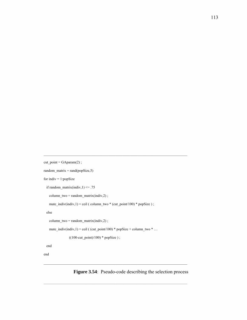
113
_______________________________________________________________________________
cut_point = GAparam(2) ;
random_matrix = rand(popSize,5)
for indiv = 1:popSize
if random_matrix(indiv,1) <= .75
column_two = random_matrix(indiv,2) ;
mate_indiv(indiv,1) = ceil ( column_two * (cut_point/100) * popSize ) ;
else
column_two = random_matrix(indiv,2) ;
mate_indiv(indiv,1) = ceil ( (cut_point/100) * popSize + column_two * …
((100-cut_point)/100) * popSize ) ;
end
end
_______________________________________________________________________________
Figure 3.54: Pseudo-code describing the selection process
_______________________________________________________________________________
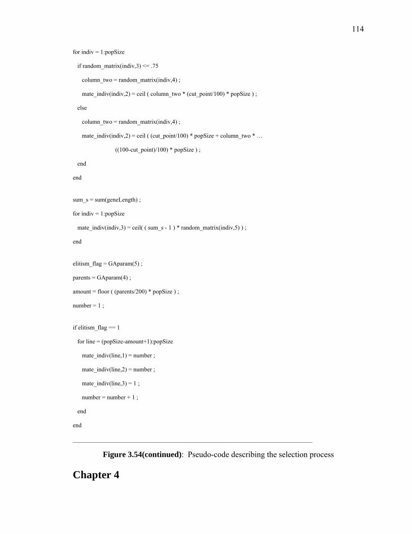
114
for indiv = 1:popSize
if random_matrix(indiv,3) <= .75
column_two = random_matrix(indiv,4) ;
mate_indiv(indiv,2) = ceil ( column_two * (cut_point/100) * popSize ) ;
else
column_two = random_matrix(indiv,4) ;
mate_indiv(indiv,2) = ceil ( (cut_point/100) * popSize + column_two * …
((100-cut_point)/100) * popSize ) ;
end
end
sum_s = sum(geneLength) ;
for indiv = 1:popSize
mate_indiv(indiv,3) = ceil( ( sum_s - 1 ) * random_matrix(indiv,5) ) ;
end
elitism_flag = GAparam(5) ;
parents = GAparam(4) ;
amount = floor ( (parents/200) * popSize ) ;
number = 1 ;
if elitism_flag == 1
for line = (popSize-amount+1):popSize
mate_indiv(line,1) = number ;
mate_indiv(line,2) = number ;
mate_indiv(line,3) = 1 ;
number = number + 1 ;
end
end
_______________________________________________________________________________
Figure 3.54(continued): Pseudo-code describing the selection process
Chapter 4

115
Design Checks for Constraint Evaluation
The constraints in the structural optimization problem are included in the MATLAB
routines as “design checks”. There are a significant number of design checks needed to
ensure that the GA solutions are feasible. The design checks are summarized in the
following sections.
4.1 Shear force and bending moment capacities of the composite beam section
Checks for shear force and bending moment in the composite beam section will be
summarized first. These two checks occur in the function vmCheck, which is utilized in
the function allChecks. Pseudo-code related to these two checks is included in Figure
4.1. To begin, relevant problem data is imported into the function vmCheck from two
main sources. Problem data like beam length, girder length, and loading intensities are
obtained from the array sysIn which was established in the function master. Properties
specific to each individual solution, like beam and girder self-weight, number of bays,
and concrete slab weight, are obtained from the array allProps which was established in
the function decodeChromo. A more detailed description of these properties can be
found in Figure 4.1.
The factored shear force and bending moment in the beam section due to factored
loading conditions will be analyzed first. The tributary width for the beams is,
gb
Ltrib
nBays= (4.1)
which has units of feet. The line load on the beam (kips/in) js,
[ ]1.2 ( ) 1.612000
b b slab deck bb
wt trib DL wt wt trib LLline
⋅ + ⋅ + + + ⋅ ⋅= (4.2)
116
where bwt is in pounds per foot and DL, LL, slabwt , and deckwt are in pounds per square
foot. The maximum shear force in the beam, ubV , is calculated according to,
122
bub
line LV ⋅ ⋅= (4.3)
in units of kips. The maximum bending moment in the beam (kip-in), ubM , is calculated
using,
2( 12)
8b
ubline LM ⋅ ⋅
= (4.4)
The effective slab width is calculated using the LRFD Manual (LRFD 2001). The
effective width be the lesser of: (a) one-eight of the beam span, center-to-center of
supports; (b) one-half the distance to the center-line of the adjacent beam; (c) the distance
to the edge of the slab. The floor panel being considered is assumed to be an interior
panel and therefore, the third condition is not considered.
The strength of a single shear stud connector, nQ , is (LRFD 2001),
0.5 'n sc c c sc uQ A f E A F= ⋅ ⋅ ≤ (4.5)
where scA is the cross-sectional area of a shear connector, 'cf is the compressive strength
of concrete in kips per square inch, cE is the modulus of elasticity of concrete in kips per
square inch, and uF is the tensile strength of steel in kips per square inch.
Next, shear connector spacing issues are addressed. rN is the number of shear
connectors positioned side-by-side in one rib at a beam intersection. The number of studs
is assumed in the present study not to exceed three, although more than three studs may
be installed (LRFD 2001). rN is used when computing the shear stud strength reduction
117
factor, R. rN will be calculated by comparing the number of shear connectors used by
each individual with the number of longitudinal shear connector locations.
The number of available shear connector locations per half beam in the
longitudinal direction, numSpots, is calculated according to,
22LnumSpots floor ⎛ ⎞= ⋅⎜ ⎟
⎝ ⎠ (4.6)
This equation is based on the fact that both the 1.5-inch deck and the 3.0-inch deck will
accept two studs per linear foot in the longitudinal direction. For the 1.5-inch deck, one
shear connector will fit in each of the two ribs which are within one linear foot. For the
3.0-inch deck, two shear connectors will fit in the single rib within one linear foot. The
actual number of shear connectors used by each individual solution, numStuds, is
compared to the value for numSpots, and a calculation is made to determine the number
of studs that will be needed to be placed side-by-side within a single deck rib at a beam
intersection. This result of this calculation indicates the value for rN .
The shear connector strength reduction factor, R, for deck ribs oriented
perpendicular to the steel beam, is given by (LRFD 2001),
0.85 1.0 1.0sr
r rr
HwRh hN
⎛ ⎞⎛ ⎞= − ≤⎜ ⎟⎜ ⎟
⎝ ⎠⎝ ⎠ (4.7)
where rN is the number of shear connectors side-by-side within a rib; rw is the average
rib width; rh is the steel deck rib height; and sH is the shear connector total length,
usually equal to the rib height plus one and one-half inches. The adjusted shear stud
118
connector strength, nrQ , is equal to the nominal connector strength, nQ times the
reduction factor, R, for deck ribs running perpendicular to the steel beam.
The adjusted moment strength, nMφ , is calculated for the composite beam section
of each individual solution. Three cases will be considered. They involve the location of
the plastic neutral axis (PNA), with the three choices being:
(1) PNA in the web of steel beam;
(2) PNA in the flange of steel beam;
(3) PNA in the concrete slab.
The calculations for each PNA location have provisions for handling fully composite and
partially composite behavior. General equations for the adjusted bending resistance of
fully and partially composite beams are provided in the LRFD Manual (LRFD 2001).
Pseudo-code related to these calculations is included in Figure 5.1. Several values must
be calculated to compute the flexural strength of the composite beam. They are given by,
p x yM Z F= ⋅ (4.8)
*
0.85 c c eC f t b= ⋅ ⋅ ⋅ (4.9)
yf f f yP b t F= ⋅ ⋅ (4.10)
y s yP A F= ⋅ (4.11)
2yweb y yfP P P= − ⋅ (4.12)
0.85
y
c e
Pa
f b=
⋅ ⋅ (4.13)
2 2cay y= − (4.14)
119
*
2y
f y
P Cy
b F−
=⋅ ⋅
(4.15)
*
2 w y
Czt F
=⋅ ⋅
(4.16)
where descriptions of individual variables are included in Figure 4.1.
The case for the plastic neutral axis (PNA) in the web of the steel beam will be
discussed first. This case applies when *
0 ywebC P≤ ≤ . The amount of studs required per
half beam for fully composite behavior is calculated as,
*
min ,yfull
nr nr
P CNQ Q
⎧ ⎫⎪ ⎪= ⎨ ⎬⎪ ⎪⎩ ⎭ (4.17)
For the case when the number of studs per half beam is greater than required amount for
fully composite behavior, the adjusted bending resistance, nMφ , is calculated according
to,
*2
20.852n p y wdM C y M F t zφ ⎡ ⎤⎛ ⎞= ⋅ ⋅ + + − ⋅ ⋅⎜ ⎟⎢ ⎥⎝ ⎠⎣ ⎦ (4.18)
where d is the depth of the steel member; 2y is the distance from the top of the steel
section to the mid-point of the stress block; pM is defined as equation (4.8); and z is the
distance from mid-depth on the steel section to the location of the PNA.
For the case when the number of shear connectors per half beam is not sufficient
to develop fully composite behavior, the same equation for nMφ is used but

120
with nrC N Q= ⋅ , where N is the number of studs per half beam. The quantities: a , 2y ,
and z would also be changed as follows,
0.85
nr
c e
N Qaf b
⋅=
⋅ ⋅ (4.19)
2 2cay y= − (4.20)
2
nr
w y
N Qzt f⋅
=⋅ ⋅
. (4.21)
The second case occurs when *
yweb yP C P≤ ≤ . This case has the PNA in the flange
of the beam section. As before, the amount of studs required per half beam for fully
composite behavior is calculated as,
*
min ,yfull
nr nr
P CNQ Q
⎧ ⎫⎪ ⎪= ⎨ ⎬⎪ ⎪⎩ ⎭
(4.22)
For the case when the number of studs per half beam is greater than required amount for
fully composite behavior, the adjusted bending resistance, nMφ , is calculated according
to,
*
20.852 2n yy d yM C y Pφ ⎡ − ⎤⎛ ⎞ ⎛ ⎞= ⋅ ⋅ + + ⋅⎜ ⎟ ⎜ ⎟⎢ ⎥⎝ ⎠ ⎝ ⎠⎣ ⎦
(4.23)
where variable definitions have been provided earlier. For the case when the number of
shear connectors per half beam is not sufficient to develop fully composite behavior, the
same equation is used but with nrC N Q= ⋅ , where N is the number of studs per half beam.
Other parameters needed for the computations are,
0.85
nr
c e
N Qaf b
⋅=
⋅ ⋅ (4.24)
121
2y nr
f
P N Qy
b fy− ⋅
=⋅ ⋅
(4.25)
2 2cay y= − . (4.26)
For the case of partially composite behavior with the PNA in the flange of the steel
section, a check is made to ensure that the value for y lies within the depth of the flange.
If y is greater than the thickness of the flange, this means that the location of the PNA
has moved down to the point where it is no longer in the flange, and is now in the web.
In this case, the equations for partially composite behavior for the PNA in the web would
apply, with nrC N Q= ⋅ .
The third case occurs when *
yP C≤ . For this case, the PNA location is within the
concrete slab. As with the two previous cases, the amount of studs required per half
beam for fully composite behavior is calculated as,
*
min ,yfull
nr nr
P CNQ Q
⎧ ⎫⎪ ⎪= ⎨ ⎬⎪ ⎪⎩ ⎭
(4.27)
For the condition when the number of studs per half beam is greater than required amount
for fully composite behavior, the adjusted bending resistance, nMφ , is calculated
according to,
20.852n ydM P yφ ⎛ ⎞= ⋅ ⋅ +⎜ ⎟
⎝ ⎠ (4.28)
where variable definitions have been provided earlier. For the condition when the
number of shear connectors per half beam is not sufficient to develop fully composite
122
behavior, an additional check must be made. It is not possible for the PNA to be in the
slab for partially composite behavior, so C must be replaced by nrN Q⋅ and the location
of the PNA must be recalculated. Depending on the location of the PNA, equations from
one of the two previous cases for partially composite behavior should be used.
Each of the three choices for PNA location include provisions for determining the
ratio, n
f
QC∑ , which is equal to the strength of shear connectors between the point of
maximum positive moment and the point of zero moment to either side divided by the
compression force in the concrete slab for fully composite behavior. These ratios are
used in determining the effective moment of inertia, effI , for a partially composite beam,
and they will be used later in the function moreCheck. A more detailed description of
these ratios can be found the LRFD Manual (LRFD 2001). Pseudo-code detailing the
values for the numerator and denominator of each ratio for each case is included in
Figure 4.1.
The value of the penalty function for bending moment in the composite beam
section is calculated as,
1ub
nb
MMφ
Φ = . (4.29)
As before, if the value for 1Φ is less than 1.0, it becomes 1.0, otherwise it remains as
defined in equation (4.29).
The shear capacity of the composite beam section includes only the strength of
the steel section and is calculated as,
123
0.9 0.6n w yV t d fφ = ⋅ ⋅ ⋅ ⋅ . (4.30)
The value for the penalty function relating to shear force in the composite beam is
calculated as,
2ub
nb
VVφ
Φ = . (4.31)
If the value for 2Φ is less than 1.0, it becomes 1.0, otherwise it remains as defined in
equation (4.31).

124
_______________________________________________________________________________
DEFINE SYSTEM AND INDIVIDUAL PROPERTIES:
% L is the beam length in feet
% W is the girder length in feet
% DL is the superimposed dead load in p.s.f.
% LL is the superimposed live load in p.s.f.
% N is the number of divisions per girder length (bays)
% beam_self_weight is the beam self weight in p.l.f.
% gird_self_weight is the girder self weight in p.l.f.
% conc_psf is the concrete slab weight in p.s.f.
% deck_psf is the steel deck weight in p.s.f.
COMPUTE FACTORED SHEAR FORCE AND BENDING MOMNET IN BEAM:
beam_trib = W / N ;
line_beam = ( 1.2 * beam_self_weight + 1.2 * beam_trib * ( DL + conc_psf ...
+ deck_psf ) + 1.6 * beam_trib * LL ) / 12000 ;
vMAXb(indiv) = ( line_beam * L * 12 ) / 2 ;
mMAXb(indiv) = ( line_beam * ( L * 12 ) ^ 2 ) / 8 ;
DEFINE SYSTEM AND INDIVIDUAL PROPERTIES:
% fc is the compressive strength of the concrete in k.s.i.
% Ec is the modulus of elasticity for the concrete in k.s.i.
% fy is the yield strength of the structural steel in k.s.i.
% Es is the modulus of elasticity for the structural steel in k.s.i.
% fu is the tensile strength of the structural steel in k.s.i.
% studDia is the diameter of the shear connectors in inches
% numStuds is the number of shear connectors per half beam
% studArea = (studDia/2)^2 * pi ;
_______________________________________________________________________________
Figure 4.1: Pseudo-code and definitions for shear and moment checks in the composite beam
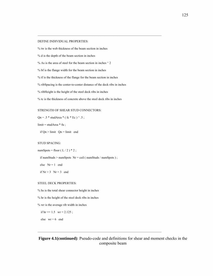
125
_______________________________________________________________________________
DEFINE INDIVIDUAL PROPERTIES:
% tw is the web thickness of the beam section in inches
% d is the depth of the beam section in inches
% As is the area of steel for the beam section in inches ^ 2
% bf is the flange width for the beam section in inches
% tf is the thickness of the flange for the beam section in inches
% ribSpacing is the center-to-center distance of the deck ribs in inches
% ribHeight is the height of the steel deck ribs in inches
% tc is the thickness of concrete above the steel deck ribs in inches
STRENGTH OF SHEAR STUD CONNECTORS:
Qn = .5 * studArea * ( fc * Ec ) ^ .5 ;
limit = studArea * fu ;
if Qn > limit Qn = limit end
STUD SPACING:
numSpots = floor ( L / 2 ) * 2 ;
if numStuds > numSpots Nr = ceil ( numStuds / numSpots ) ;
else Nr = 1 end
if Nr > 3 Nr = 3 end
STEEL DECK PROPERTIES:
% hs is the total shear connector height in inches
% hr is the height of the steel deck ribs in inches
% wr is the average rib width in inches
if hr == 1.5 wr = 2.125 ;
else wr = 6 end
_______________________________________________________________________________
Figure 4.1(continued): Pseudo-code and definitions for shear and moment checks in the composite beam

126
_______________________________________________________________________________
FIND SHEAR CONNECTOR REDUCTION FACTOR:
R = ( ( .85 * wr ) / ( (Nr^.5) * hr ) ) * ( (hs / hr) - 1 ) ;
if R > 1 R = 1 end
Qnr = R * .5 * studArea * (fc * Ec) ^ 0.5 ;
limitTwo = studArea * fu ;
if Qnr > limitTwo Qnr = limitTwo end
FIND EFFECTIVE WIDTH OF SLAB:
be1 = ( L / 8 ) * 12 ;
be2 = ( W / (N*2) ) * 12 ;
be = min(be1,be2) ;
DEFINED VALUES:
% yc = tc + ribHeight ;
% Zx is the plastic modulus with respect to strong axis bending in inches ^ 3
COMPUTED VALUES:
Mp = Zx * fy ;
C_star = .85 * fc * tc * be ;
Pyf = bf * tf * fy ;
Py = As * fy ;
Pyweb = Py - 2 * Pyf ;
a = Py / ( .85 * fc * be ) ;
if a > tc a = tc end
y2 = yc - (a/2) ;
y_bar = ( ( Py - C_star ) / ( 2 * bf * fy ) ) ;
z_bar = ( C_star / ( 2 * tw * fy ) ) ;
N_full = min ( (Py/Qnr) , (C_star/Qnr) ) ;
_______________________________________________________________________________
Figure 4.1(continued): Pseudo-code and definitions for shear and moment checks in the composite beam
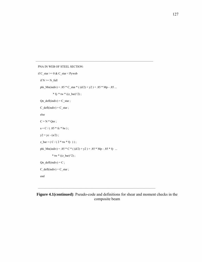
127
_______________________________________________________________________________
PNA IN WEB OF STEEL SECTION:
if C_star >= 0 & C_star < Pyweb
if N >= N_full
phi_Mn(indiv) = .85 * C_star * ( (d/2) + y2 ) + .85 * Mp - .85 ...
* fy * tw * ((z_bar)^2) ;
Qn_defl(indiv) = C_star ;
C_defl(indiv) = C_star ;
else
C = N * Qnr ;
a = C / ( .85 * fc * be ) ;
y2 = yc - (a/2) ;
z_bar = ( C / ( 2 * tw * fy ) ) ;
phi_Mn(indiv) = .85 * C * ( (d/2) + y2 ) + .85 * Mp - .85 * fy ...
* tw * ((z_bar)^2) ;
Qn_defl(indiv) = C ;
C_defl(indiv) = C_star ;
end
_______________________________________________________________________________
Figure 4.1(continued): Pseudo-code and definitions for shear and moment checks in the composite beam
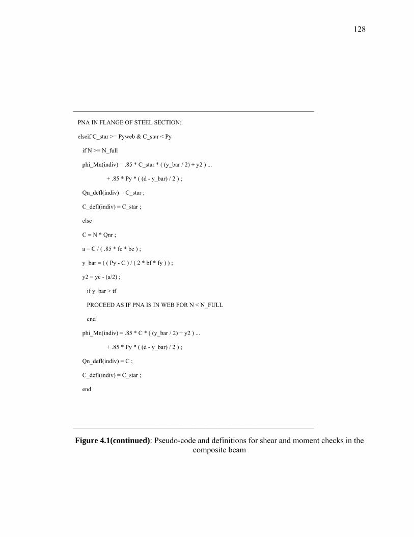
128
_______________________________________________________________________________
PNA IN FLANGE OF STEEL SECTION:
elseif C_star >= Pyweb & C_star < Py
if N >= N_full
phi_Mn(indiv) = .85 * C_star * ( (y_bar / 2) + y2 ) ...
+ .85 * Py * ( (d - y_bar) / 2 ) ;
Qn_defl(indiv) = C_star ;
C_defl(indiv) = C_star ;
else
C = N * Qnr ;
a = C / ( .85 * fc * be ) ;
y_bar = ( ( Py - C ) / ( 2 * bf * fy ) ) ;
y2 = yc - (a/2) ;
if y_bar > tf
PROCEED AS IF PNA IS IN WEB FOR N < N_FULL
end
phi_Mn(indiv) = .85 * C * ( (y_bar / 2) + y2 ) ...
+ .85 * Py * ( (d - y_bar) / 2 ) ;
Qn_defl(indiv) = C ;
C_defl(indiv) = C_star ;
end
_______________________________________________________________________________
Figure 4.1(continued): Pseudo-code and definitions for shear and moment checks in the composite beam
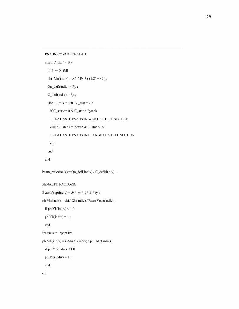
129
_______________________________________________________________________________
PNA IN CONCRETE SLAB:
elseif C_star >= Py
if N >= N_full
phi_Mn(indiv) = .85 * Py * ( (d/2) + y2 ) ;
Qn_defl(indiv) = Py ;
C_defl(indiv) = Py ;
else C = N * Qnr C_star = C ;
if C_star >= 0 & C_star < Pyweb
TREAT AS IF PNA IS IN WEB OF STEEL SECTION
elseif C_star >= Pyweb & C_star < Py
TREAT AS IF PNA IS IN FLANGE OF STEEL SECTION
end
end
end
beam_ratio(indiv) = Qn_defl(indiv) / C_defl(indiv) ;
PENALTY FACTORS:
BeamVcap(indiv) = .9 * tw * d *.6 * fy ;
phiVb(indiv) = vMAXb(indiv) / BeamVcap(indiv) ;
if phiVb(indiv) < 1.0
phiVb(indiv) = 1 ;
end
for indiv = 1:popSize
phiMb(indiv) = mMAXb(indiv) / phi_Mn(indiv) ;
if phiMb(indiv) < 1.0
phiMb(indiv) = 1 ;
end
end
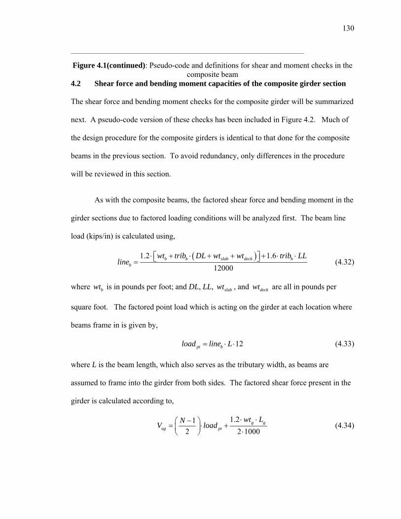
130
_______________________________________________________________________________
Figure 4.1(continued): Pseudo-code and definitions for shear and moment checks in the composite beam
4.2 Shear force and bending moment capacities of the composite girder section
The shear force and bending moment checks for the composite girder will be summarized
next. A pseudo-code version of these checks has been included in Figure 4.2. Much of
the design procedure for the composite girders is identical to that done for the composite
beams in the previous section. To avoid redundancy, only differences in the procedure
will be reviewed in this section.
As with the composite beams, the factored shear force and bending moment in the
girder sections due to factored loading conditions will be analyzed first. The beam line
load (kips/in) is calculated using,
( )1.2 1.6
12000b b slab deck b
b
wt trib DL wt wt trib LLline
⋅ + ⋅ + + + ⋅ ⋅⎡ ⎤⎣ ⎦= (4.32)
where bwt is in pounds per foot; and DL, LL, slabwt , and deckwt are all in pounds per
square foot. The factored point load which is acting on the girder at each location where
beams frame in is given by,
12pt bload line L= ⋅ ⋅ (4.33)
where L is the beam length, which also serves as the tributary width, as beams are
assumed to frame into the girder from both sides. The factored shear force present in the
girder is calculated according to,
1.21
2 2 1000g g
ug pt
wt LNV load⋅ ⋅−⎛ ⎞= ⋅ +⎜ ⎟ ⋅⎝ ⎠
(4.34)

131
where N is the number of divisions per girder length. The factored bending moment
present in the girder is calculated using,
( )21.2 12
1212000 8
gug pt g
wt WM C load L
⋅ ⋅ ⋅= + ⋅ ⋅ ⋅
⋅ (4.35)
where C is a constant taken from the LRFD Manual (LRFD 1998). Values for C are
shown in Figure 4.2.
The shear connector strength reduction factor, R, for deck ribs oriented parallel to
the steel girder, is given by LRFD Equation (I3-2) p. 16.1-45 (LRFD 2001),
0.6 1.0 1.0sr
r r
HwRh h
⎛ ⎞ ⎛ ⎞= ⋅ ⋅ − ≤⎜ ⎟ ⎜ ⎟
⎝ ⎠ ⎝ ⎠ (4.36)
where rw is the average rib width; rh is the steel deck rib height; and sH is the shear
connector total length (usually equal to the rib height plus one and one-half inches). The
adjusted shear stud connector strength, nrQ , is equal to the nominal connector strength,
nQ times the reduction factor, R, for deck ribs running parallel to the steel girder.
Shear and moment capacities for the composite girder are calculated using the
same equations as were used for the composite beam. The value of the penalty function
for bending moment in the composite girder section is calculated as,
3ug
ng
MMφ
Φ = (4.37)
As before, if the value for 3Φ is less than 1.0, it becomes 1.0, otherwise it remains as
defined in equation (4.37). The value for the penalty function relating to shear force in
the composite girder is calculated as,
132
4ug
ng
VVφ
Φ = (4.38)
If the value for 4Φ is less than 1.0, it becomes 1.0, otherwise it remains as defined in
equation (4.38).
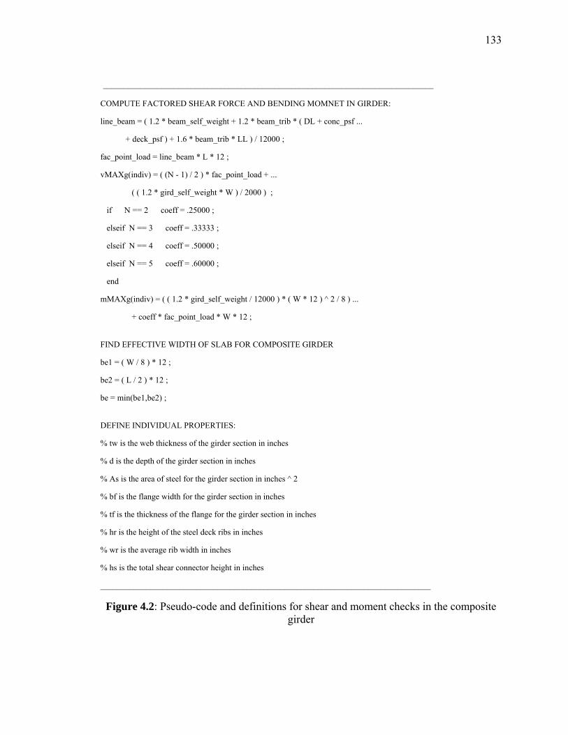
133
_______________________________________________________________________________
COMPUTE FACTORED SHEAR FORCE AND BENDING MOMNET IN GIRDER:
line_beam = ( 1.2 * beam_self_weight + 1.2 * beam_trib * ( DL + conc_psf ...
+ deck_psf ) + 1.6 * beam_trib * LL ) / 12000 ;
fac_point_load = line_beam * L * 12 ;
vMAXg(indiv) = ( (N - 1) / 2 ) * fac_point_load + ...
( ( 1.2 * gird_self_weight * W ) / 2000 ) ;
if N == 2 coeff = .25000 ;
elseif N == 3 coeff = .33333 ;
elseif N == 4 coeff = .50000 ;
elseif N == 5 coeff = .60000 ;
end
mMAXg(indiv) = ( ( 1.2 * gird_self_weight / 12000 ) * ( W * 12 ) ^ 2 / 8 ) ...
+ coeff * fac_point_load * W * 12 ;
FIND EFFECTIVE WIDTH OF SLAB FOR COMPOSITE GIRDER
be1 = ( W / 8 ) * 12 ;
be2 = ( L / 2 ) * 12 ;
be = min(be1,be2) ;
DEFINE INDIVIDUAL PROPERTIES:
% tw is the web thickness of the girder section in inches
% d is the depth of the girder section in inches
% As is the area of steel for the girder section in inches ^ 2
% bf is the flange width for the girder section in inches
% tf is the thickness of the flange for the girder section in inches
% hr is the height of the steel deck ribs in inches
% wr is the average rib width in inches
% hs is the total shear connector height in inches
_______________________________________________________________________________
Figure 4.2: Pseudo-code and definitions for shear and moment checks in the composite girder

134
_______________________________________________________________________________ FIND REDUCTION FACTOR FOR RIBS ORIENTED PARALLEL TO GIRDER:
R = ( (.6 * wr) / hr ) * ( (hs / hr) - 1 ) ;
if R > 1 R = 1 end
FIND ADJUSTED STRENGTH FOR EACH SHEAR STUD CONNECTOR:
Qnr = R * Qn ;
limit = studArea * fu ;
if Qnr > limit
Qnr = limit
end
PNA IN WEB OF STEEL SECTION:
if C_star >= 0 & C_star < Pyweb
if N >= N_full
phi_Mng(indiv) = .85 * C_star * ( (d/2) + y2 ) + .85 ...
* Mp - .85 * fy * tw * ((z_bar)^2) ;
Qn_defl(indiv) = C_star ;
C_defl(indiv) = C_star ;
else
C = N * Qnr ;
a = C / ( .85 * fc * be ) ;
y2 = yc - (a/2) ;
z_bar = ( C / ( 2 * tw * fy ) ) ;
phi_Mng(indiv) = .85 * C * ( (d/2) + y2 ) + .85 * Mp ...
- .85 * fy * tw * ((z_bar)^2) ;
Qn_defl(indiv) = C ;
C_defl(indiv) = C_star ;
end
_______________________________________________________________________________
Figure 4.2(continued): Pseudo-code and definitions for shear and moment checks in the composite girder

135
_______________________________________________________________________________
PNA IN FLANGE OF STEEL SECTION:
elseif C_star >= Pyweb & C_star < Py
if N >= N_full
phi_Mng(indiv) = .85 * C_star * ( (y_bar / 2) + y2 ) ...
+ .85 * Py * ( (d - y_bar) / 2 ) ;
Qn_defl(indiv) = C_star ;
C_defl(indiv) = C_star ;
else
C = N * Qnr ;
a = C / ( .85 * fc * be ) ;
y_bar = ( ( Py - C ) / ( 2 * bf * fy ) ) ;
y2 = yc - (a/2) ;
if y_bar > tf
PROCEED AS IF PNA IS IN WEB FOR N < N_FULL
end
phi_Mng(indiv) = .85 * C * ( (y_bar / 2) + y2 ) ...
+ .85 * Py * ( (d - y_bar) / 2 ) ;
Qn_defl(indiv) = C ;
C_defl(indiv) = C_star ;
end
_______________________________________________________________________________
Figure 4.2(continued): Pseudo-code and definitions for shear and moment checks in the composite girder
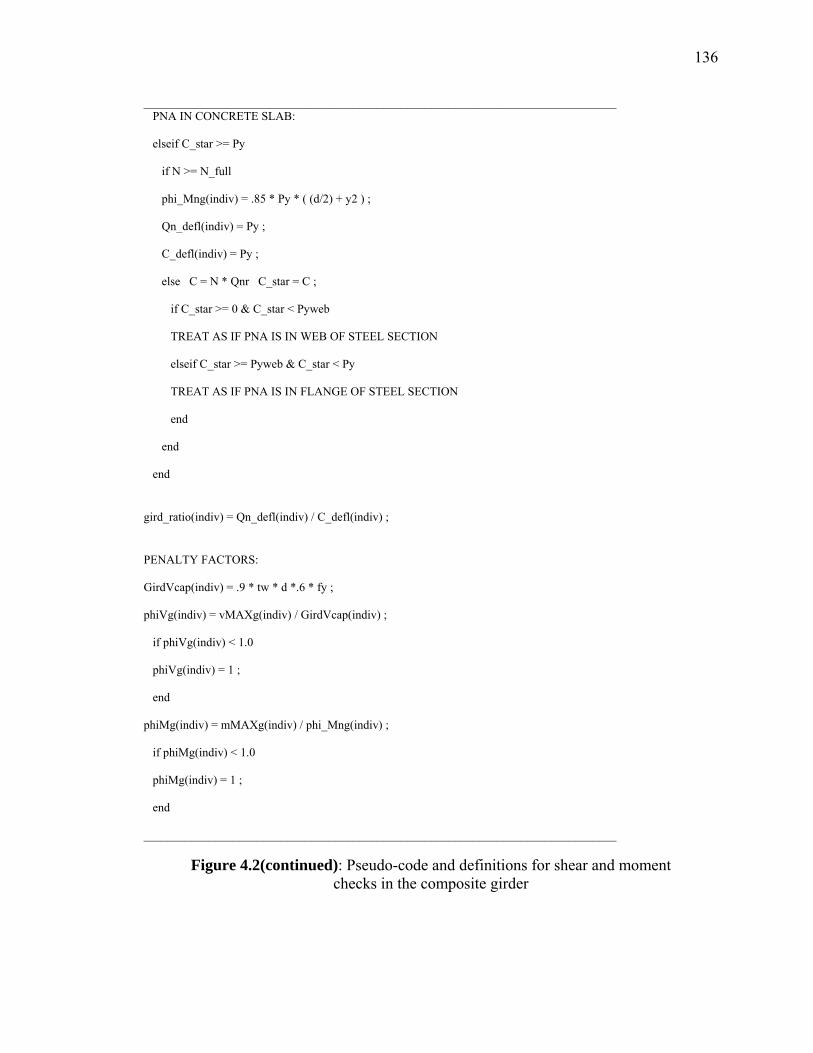
136
_______________________________________________________________________________ PNA IN CONCRETE SLAB:
elseif C_star >= Py
if N >= N_full
phi_Mng(indiv) = .85 * Py * ( (d/2) + y2 ) ;
Qn_defl(indiv) = Py ;
C_defl(indiv) = Py ;
else C = N * Qnr C_star = C ;
if C_star >= 0 & C_star < Pyweb
TREAT AS IF PNA IS IN WEB OF STEEL SECTION
elseif C_star >= Pyweb & C_star < Py
TREAT AS IF PNA IS IN FLANGE OF STEEL SECTION
end
end
end
gird_ratio(indiv) = Qn_defl(indiv) / C_defl(indiv) ;
PENALTY FACTORS:
GirdVcap(indiv) = .9 * tw * d *.6 * fy ;
phiVg(indiv) = vMAXg(indiv) / GirdVcap(indiv) ;
if phiVg(indiv) < 1.0
phiVg(indiv) = 1 ;
end
phiMg(indiv) = mMAXg(indiv) / phi_Mng(indiv) ;
if phiMg(indiv) < 1.0
phiMg(indiv) = 1 ;
end
_______________________________________________________________________________
Figure 4.2(continued): Pseudo-code and definitions for shear and moment checks in the composite girder
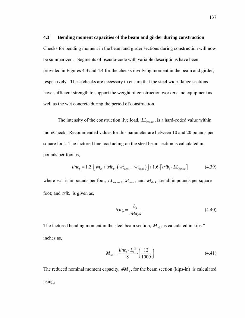
137
4.3 Bending moment capacities of the beam and girder during construction
Checks for bending moment in the beam and girder sections during construction will now
be summarized. Segments of pseudo-code with variable descriptions have been
provided in Figures 4.3 and 4.4 for the checks involving moment in the beam and girder,
respectively. These checks are necessary to ensure that the steel wide-flange sections
have sufficient strength to support the weight of construction workers and equipment as
well as the wet concrete during the period of construction.
The intensity of the construction live load, constrLL , is a hard-coded value within
moreCheck. Recommended values for this parameter are between 10 and 20 pounds per
square foot. The factored line load acting on the steel beam section is calculated in
pounds per foot as,
( ) [ ]1.2 1.6b b b deck conc b constrline wt trib wt wt trib LL= ⋅ + ⋅ + + ⋅ ⋅⎡ ⎤⎣ ⎦ (4.39)
where bwt is in pounds per foot; constrLL , concwt , and deckwt are all in pounds per square
foot; and btrib is given as,
gb
Ltrib
nBays= . (4.40)
The factored bending moment in the steel beam section, ubM , is calculated in kips *
inches as,
2 12
8 1000b b
ubline LM ⋅ ⎛ ⎞= ⋅⎜ ⎟
⎝ ⎠ (4.41)
The reduced nominal moment capacity, nMφ , for the beam section (kips-in) is calculated
using,
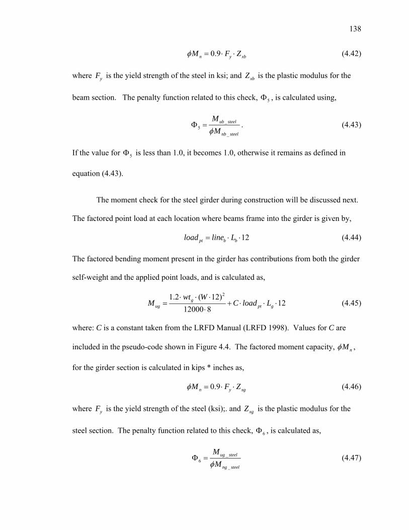
138
0.9n y xbM F Zφ = ⋅ ⋅ (4.42)
where yF is the yield strength of the steel in ksi; and xbZ is the plastic modulus for the
beam section. The penalty function related to this check, 5Φ , is calculated using,
_5
_
ub steel
nb steel
MMφ
Φ = . (4.43)
If the value for 5Φ is less than 1.0, it becomes 1.0, otherwise it remains as defined in
equation (4.43).
The moment check for the steel girder during construction will be discussed next.
The factored point load at each location where beams frame into the girder is given by,
12pt b bload line L= ⋅ ⋅ (4.44)
The factored bending moment present in the girder has contributions from both the girder
self-weight and the applied point loads, and is calculated as,
21.2 ( 12)
1212000 8
gug pt g
wt WM C load L
⋅ ⋅ ⋅= + ⋅ ⋅ ⋅
⋅ (4.45)
where: C is a constant taken from the LRFD Manual (LRFD 1998). Values for C are
included in the pseudo-code shown in Figure 4.4. The factored moment capacity, nMφ ,
for the girder section is calculated in kips * inches as,
0.9n y xgM F Zφ = ⋅ ⋅ (4.46)
where yF is the yield strength of the steel (ksi);. and xgZ is the plastic modulus for the
steel section. The penalty function related to this check, 6Φ , is calculated as,
_6
_
ug steel
ng steel
MMφ
Φ = (4.47)
139
If the value for 6Φ is less than 1.0, it becomes 1.0, otherwise it remains as defined in
equation (4.47).
4.4 Deflection of the composite beam and the composite girder Checks for deflection of the composite beam and composite girder will now be
summarized. Segments of pseudo-code with variable descriptions have been provided in
Figures 4.5 and 4.6. In order to begin the composite beam deflection checks, appropriate
problem data must be collected. System properties, such as beam length, girder length,
and superimposed dead load, are obtained from the function master, where they were
established by the program user. Individual properties, such as number of divisions per
girder length and self-weight of the beam section, are taken from the array allProps which
was created in the function decodeChromo.
The effective slab width is calculated next according to provisions from Section
I3.1 of p. 16.1-43 of the LRFD Manual (LRFD 2001). The section recommends that the
effective width, eb , be the lesser of: (a) one-eight of the beam span, center-to-center of
supports; (b) one-half the distance to the center-line of the adjacent beam; (c) the
distance to the edge of the slab. As the floor panel being considered is assumed to be an
interior panel, the third condition has not been included as an option. The modulus of
elasticity ratio, n, is next calculated according to,
s
c
EnE
= (4.48)

140
_______________________________________________________________________________ DEFINE SYSTEM PROPERTIES:
% W is the girder length in feet
% L is the beam length in feet
% fy is the yield strength of steel in k.s.i.
DEFINE INDIVIDUAL PROPERTIES:
% wtDeck is the weight of the steel decking in p.s.f.
% wtConc is the weight of the concrete slab in p.s.f.
% wtBeam is the self-weight of the beam in pounds per linear foot
% wtGird is the self-weight of the girder in pounds per linear foot
% bays is the number of divisions per girder length
% ZxBeam is the plastic modulus for the beam section in inches ^ 3
% ZxGird is the plastic modulus for the girder section in inches ^ 3
HARD-CODED VALUES:
% wtConstr is the chosen construction live load value in p.s.f.
FIND Mu:
tribLength = W / bays ;
lineLoad = 1.2 * tribLength * (wtConc+wtDeck) + 1.2 * wtBeam + 1.6 * tribLength
* wtConstr ;
MuBeam(indiv) = ( ( lineLoad * L * L ) / 8 ) * ( 12 / 1000 ) ;
FIND phiMn:
facBeamCap(indiv) = .9 * Fy * ZxBeam ;
ESTABLISH PENALTY:
beamAlone(indiv) = MuBeam(indiv) / facBeamCap(indiv) ;
if beamAlone(indiv) < 1
beamAlone(indiv) = 1 ;
end
_______________________________________________________________________________
Figure 4.3: Pseudo-code for bending moment check in the beam during construction

141
_______________________________________________________________________________
VARIABLES ALREADY DEFINED IN FIGURE 3
FIND Mu:
line_from_beam = ( 1.2 * wtBeam + 1.2 * tribLength * ( wtDeck + wtConc )
+ 1.6 * tribLength * wtConstr ) / 12000 ;
fac_point_load = line_from_beam * L * 12 ;
if bays == 2 coeff = .250 ;
elseif bays == 3 coeff = .333 ;
elseif bays == 4 coeff = .500 ;
elseif bays == 5 coeff = .600 ;
end
MuGird(indiv) = ( ( ( 1.2 * wtGird ) / 12000 ) * ( W * 12 ) ^ 2 / 8 )
+ coeff * fac_point_load * W * 12 ;
FIND phiMn:
facGirdCap(indiv) = .9 * Fy * ZxGird ;
ESTABLISH PENALTY:
girdAlone(indiv) = MuGird(indiv) / facGirdCap(indiv) ;
if girdAlone(indiv) < 1
girdAlone(indiv) = 1 ;
end
_______________________________________________________________________________
Figure 4.4: Pseudo-code for bending moment check in the girder during construction

142
The modified effective width _e newb is calculated according to,
_e
e newbbn
= . (4.49)
The modified effective width value, _e newb , is used to convert the cross-sectional area of
the concrete slab into an equivalent area of steel. In later calculations, _e newb will be
replaced by eb for simplicity.
Next, the procedure for finding the effective moment of inertia for the composite
cross-section, effI , will be summarized. The distance up from the centroidal axis of the
steel section to the centroidal axis of the fully composite, uncracked transformed section,
updist , is calculated in inches according to,
2 2
e c cup r
s e c
b t t ddist hA b t
⋅ ⎛ ⎞= ⋅ + +⎜ ⎟+ ⋅ ⎝ ⎠ (4.50)
The process for obtaining this equation can be seen in Appendix C. Next, the distance
down from the transformed concrete centroidal axis to the centroidal axis of the fully
composite uncracked transformed section, downdist , is calculated is inches as,
2 2c
down r upt ddist h dist⎛ ⎞= + + −⎜ ⎟
⎝ ⎠. (4.51)
The transformed, uncracked moment of inertia, trI , is calculated as,
2 3 2112tr st s up e c e c downI I A dist b t b t dist= + ⋅ + ⋅ ⋅ + ⋅ ⋅ . (4.52)
143
The effective moment of inertia for a partially composite beam, effI , is approximated
using standard procedures (LRFD 2001),
( )neff s tr s
f
QI I I I
C= + ⋅ −∑ . (4.53)
where: sI is the moment of inertia for the structural steel section; nQ∑ is the strength
of the shear connectors between the point of maximum positive moment and the point of
zero moment to either side in kips; and fC is the compression force in the concrete slab
for fully composite behavior (kips). The ratio n
f
QC∑ will be equal to 1.0 for fully
composite behavior and will be less than 1.0 for partially composite behavior. For the
case where n
f
QC∑ is equal to 1.0, it can be seen that effI will simply equal trI , as would
be expected. Values for nQ∑ and fC are collected during the moment strength check
in the function vmCheck. They are carried in the first column of an array called ratios.
With effI calculated, the next step is to determine the line load on the beam. Only
superimposed live load and superimposed dead load will be considered for this check.
Service loads will be used with no load factors applied. Self-weight of the structure has
not been considered as it was used in determining construction deflections that have
either been reduced due to cambering or leveled off with the addition of more concrete.
The beam line load, bline , is calculated in kips per foot as,
( )12 1000
bb
trib sLL sDLline ⋅ +=
⋅ (4.54)

144
The composite beam deflection is calculated in inches as,
45 ( 12)
384b b
bs eff
line LE I
δ ⋅ ⋅ ⋅=
⋅ ⋅ (4.55)
and the deflection limit in inches is defined as,
max12bL
Aδ ⋅
= (4.56)
where A is a value chosen by the user, usually 240 to 400. The penalty function related
to this check, 7Φ , is calculated as,
7max
bδδ
Φ = (4.57)
If the value for 7Φ is less than 1.0, it becomes 1.0, otherwise it remains as defined in
equation (4.57).
The calculation for deflection of the composite girder is very similar to that of the
composite beam. Pseudo-code for the composite girder deflection check has been
included in Figure 4.6. As many of the steps are identical to those for the beam
deflection, only differences will be summarized in this section. Most of the differences
arise because the steel girder’s length is parallel to the deck ribs, and not perpendicular as
with the beam. The concrete in the ribs of the deck above the girder is not included in
strength calculations, but is included in calculations for deflection. The omission of
concrete in the ribs makes the strength calculations conservative, which is acceptable for
the design. In contrast, the deflection check is supposed to represent actual building
conditions, so loads are not factored, and the true composite cross-section included
concrete within the ribs will be considered.
145
The effective width of the concrete above the deck ribs is determined as for the
beam. But additionally, the effective width of concrete within the ribs will be considered
as 2eb , and calculated as,
2_ _
12e ewidth per footb b ⎛ ⎞= ⋅⎜ ⎟
⎝ ⎠ (4.58)
where width_per_foot is the average concrete width within the ribs per foot of effective
width. As before, the modular ratio, n, is next calculated,
s
c
EnE
= (4.59)
and the modified effective width 2 _e newb is calculated using,
22_
ee new
bbn
= (4.60)
The modified effective width value, 2 _e newb , is used to convert the cross-sectional area of
the concrete within the ribs into an equivalent area of steel. In later calculations, 2 _e newb
will be replaced by 2eb for simplicity.
The distance up from the centroidal axis of the steel section to the centroidal axis
of the fully composite uncracked transformed section, updist , will be calculated in inches
according to,
2
2
2 2 2 2c r
e c r e r
ups e c e
t hd db t h b hdist
A b t b h
⎛ ⎞ ⎛ ⎞⋅ ⋅ + + + ⋅ ⋅ +⎜ ⎟⎜ ⎟⎝ ⎠⎝ ⎠=
+ ⋅ + ⋅ . (4.61)

146
The process for obtaining this equation can be seen as Appendix C. Next, the distance
down from the transformed concrete centroidal axis (concrete above ribs only) to the
centroidal axis of the fully composite uncracked transformed section, downdist , is,
2 2c
down r upt ddist h dist⎛ ⎞= + + −⎜ ⎟
⎝ ⎠ (4.62)
and the distance from the centroidal axis of the concrete within the ribs, ribsdist , is given
in inches as,
2 2r
ribs uph ddist dist= + − (4.63)
The transformed uncracked moment of inertia, trI , is calculated in inches4 according to,
2 3 2 3 22 2
1 112 12tr s s up e c e c down e r e r ribsI I A dist b t b t dist b h b h dist= + ⋅ + ⋅ ⋅ + ⋅ ⋅ + ⋅ ⋅ + ⋅ ⋅ (4.64)
The effective moment of inertia for a partially composite beam, effI , is approximated as
before.
An assumption was made when calculating the maximum deflection for the
composite girder section after construction. It was assumed that the superimposed live
load and superimposed dead load were applied in a uniform way over the length of the
girder, instead of a number of point loads acting at the locations where the beams frame
into the girder. The number of point loads varies for each individual solution as the
number of divisions per girder length changes. This fact makes the deflection calculation
more difficult, and so it was decided to use the loading assumption described earlier. As
can be seen in Appendix B, this assumption provides conservative results by 3.3% to
25.0%. For the geometry that includes five divisions per girder length, the assumption
147
provides results that are the least conservative, only 3.3%. For the case where there are
only two divisions per girder length, the assumption provides results that are the most
conservative, 24.0%.
The girder line load, gline , (kips/ft) associated with the previously mentioned
assumption is calculated as,
( )
12 1000g
g
trib sLL sDLline
⋅ +=
⋅ (4.65)
and girder deflection and deflection limit are calculated as before.
The penalty function related to this check, 8Φ , is calculated as,
8max
gδδ
Φ = (4.66)
If the value for 8Φ is less than 1.0, it becomes 1.0, otherwise it remains as defined in
equation (4.66).
4.5 Deflection of the beam and girder during construction The procedure for calculating deflections of the beam and girder during construction will be summarized in this section. Segments of pseudo-code used in determining beam and girder deflections can be seen in Figures 4.7 and 4.8, respectively.
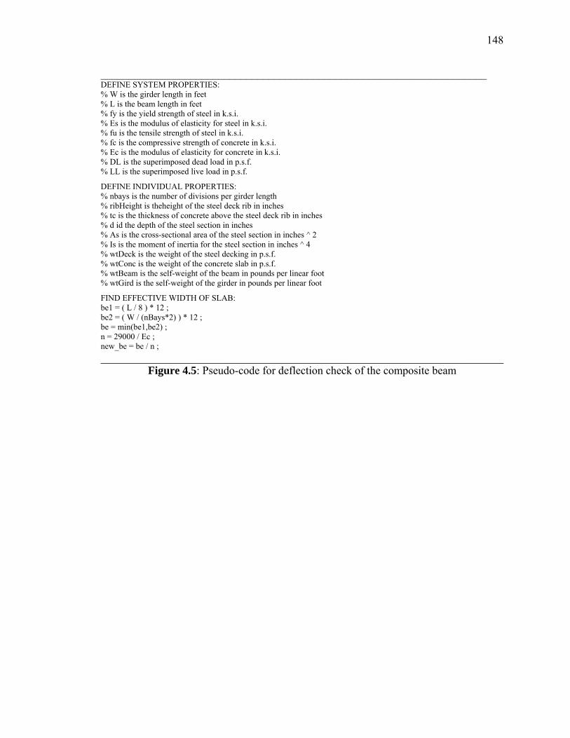
148
_____________________________________________________________________ DEFINE SYSTEM PROPERTIES: % W is the girder length in feet % L is the beam length in feet % fy is the yield strength of steel in k.s.i. % Es is the modulus of elasticity for steel in k.s.i. % fu is the tensile strength of steel in k.s.i. % fc is the compressive strength of concrete in k.s.i. % Ec is the modulus of elasticity for concrete in k.s.i. % DL is the superimposed dead load in p.s.f. % LL is the superimposed live load in p.s.f.
DEFINE INDIVIDUAL PROPERTIES: % nbays is the number of divisions per girder length % ribHeight is theheight of the steel deck rib in inches % tc is the thickness of concrete above the steel deck rib in inches % d id the depth of the steel section in inches % As is the cross-sectional area of the steel section in inches ^ 2 % Is is the moment of inertia for the steel section in inches ^ 4 % wtDeck is the weight of the steel decking in p.s.f. % wtConc is the weight of the concrete slab in p.s.f. % wtBeam is the self-weight of the beam in pounds per linear foot % wtGird is the self-weight of the girder in pounds per linear foot
FIND EFFECTIVE WIDTH OF SLAB: be1 = ( L / 8 ) * 12 ; be2 = ( W / (nBays*2) ) * 12 ; be = min(be1,be2) ; n = 29000 / Ec ; new_be = be / n ; ________________________________________________________________________
Figure 4.5: Pseudo-code for deflection check of the composite beam

149
________________________________________________________________________
FIND DISTANCE:
distance_up = (( new_be * tc )/( As + new_be * tc ))*( tc/2 + ribHeight + d/2);
distance = ( tc / 2 ) + ribHeight + ( d / 2 ) ;
distance_down = distance - distance_up ;
FIND Ieff:
Itr = Is + As * distance_up^2 + (1/12) * new_be * tc^3 + new_be * tc ...
* distance_down^2 ;
bRatio = ratios(1,indiv) ;
Ieff = Is + ( bRatio^.5 ) * ( Itr - Is ) ;
FIND DEFLECTION AND LIMIT:
tribLength = W / nBays ;
w = (tribLength * (DL+LL) ) / 12000 ;
defl_beam(indiv) = ( 5 * w * (L*12)^4 ) / ( 384 * E * Ieff ) ;
defl_b_limit(indiv) = L * 12 / 360 ;
ESTABLISH PENALTY:
deflBeam(indiv) = defl_beam(indiv) / defl_b_limit(indiv) ;
if deflBeam(indiv) < 1
deflBeam(indiv) = 1 ;
end
________________________________________________________________________
Figure 4.5(continued): Pseudo-code for deflection check of the composite beam
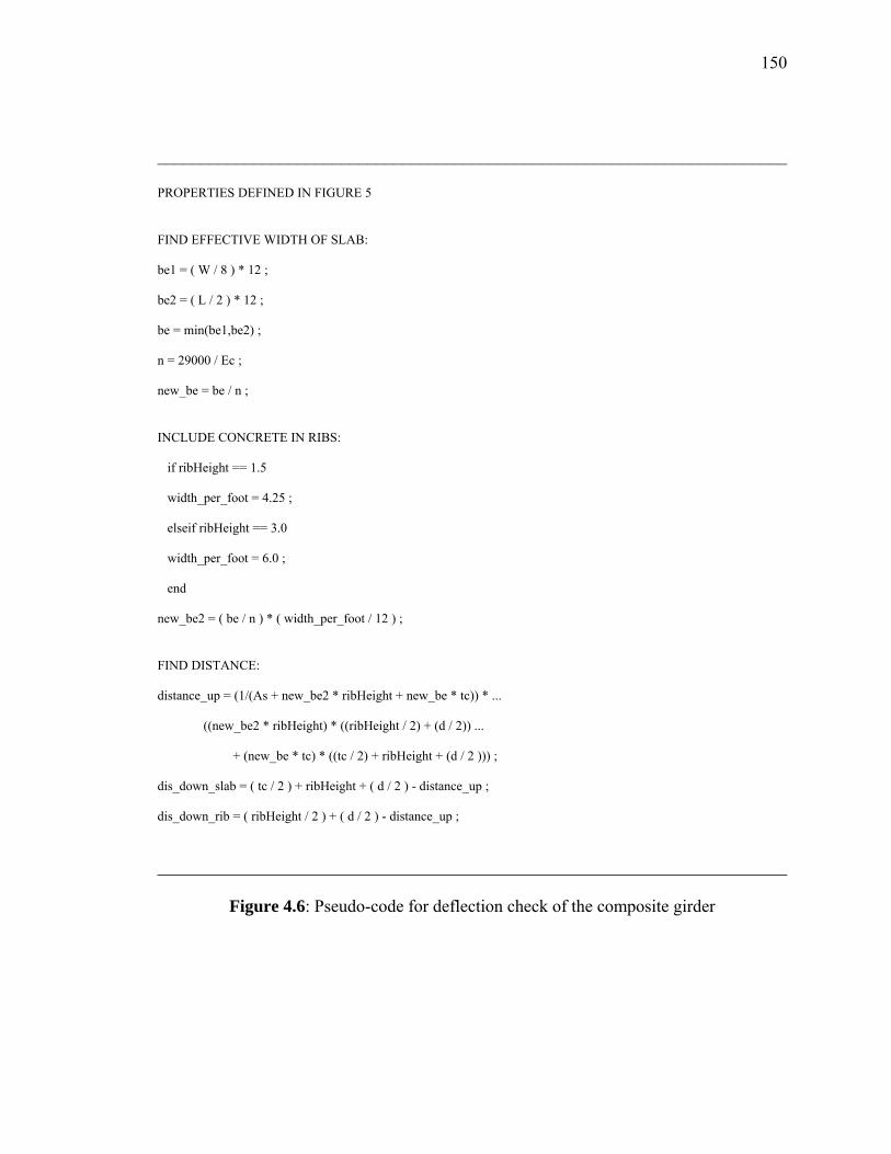
150
________________________________________________________________________
PROPERTIES DEFINED IN FIGURE 5
FIND EFFECTIVE WIDTH OF SLAB:
be1 = ( W / 8 ) * 12 ;
be2 = ( L / 2 ) * 12 ;
be = min(be1,be2) ;
n = 29000 / Ec ;
new_be = be / n ;
INCLUDE CONCRETE IN RIBS:
if ribHeight == 1.5
width_per_foot = 4.25 ;
elseif ribHeight == 3.0
width_per_foot = 6.0 ;
end
new_be2 = ( be / n ) * ( width_per_foot / 12 ) ;
FIND DISTANCE:
distance_up = (1/(As + new_be2 * ribHeight + new_be * tc)) * ...
((new_be2 * ribHeight) * ((ribHeight / 2) + (d / 2)) ...
+ (new_be * tc) * ((tc / 2) + ribHeight + (d / 2 ))) ;
dis_down_slab = ( tc / 2 ) + ribHeight + ( d / 2 ) - distance_up ;
dis_down_rib = ( ribHeight / 2 ) + ( d / 2 ) - distance_up ;
________________________________________________________________________
Figure 4.6: Pseudo-code for deflection check of the composite girder

151
________________________________________________________________________
FIND Ieff:
Itr = Is + As * distance_up^2 + (1/12) * new_be * tc^3 + new_be * tc ...
* dis_down_slab^2 + (1/12) * new_be2 * ribHeight^3 + new_be2 ...
* ribHeight * dis_down_rib^2;
gRatio = ratios(2,indiv) ;
Ieff = Is + ( gRatio^.5 ) * ( Itr - Is ) ;
FIND DEFLECTION AND LIMIT:
w = ( tribLength * (DL+LL) ) / 12000 ;
defl_gird(indiv) = ( 5 * w * (L*12)^4 ) / ( 384 * E * Ieff ) ;
defl_g_limit(indiv) = L*12 / 360 ;
deflGird(indiv) = defl_gird(indiv) / defl_g_limit(indiv) ;
if deflGird(indiv) < 1
deflGird(indiv) = 1 ;
end
________________________________________________________________________
Figure 4.6(continued): Pseudo-code for deflection check of the composite girder
The calculations for beam and girder deflections are useful in identifying framing
configurations where excessive ponding of concrete during construction might occur.
Excessive ponding results when the deflection of a steel member is so large that even
more concrete must be used to level the slab. The addition of more concrete leads to
additional deflection, and so it is desirable to try and limit deflection caused by ponding
in the design phase. The beam and girder construction deflection calculations could also

152
be used in directing the steel fabricator to camber the steel members, if that choice is
made.
Deflection calculations are made using only the actual loads that are expected to
be present on the framing members during the curing of the concrete. It is assumed that
minimal workers and no equipment will be left on the floor panel during curing.
Therefore, only beam self-weight, girder self-weight, wet concrete weight, and deck
weight will be considered.
The service line load (kips/in) on the beam sections is ,
( )12 1000
b b conc deckb
wt trib wt wtline + ⋅ +=
⋅ (4.67)
where bwt is in pounds per foot; and concwt , deckwt are in pounds per square foot; and
btrib is given as,
gb
Ltrib
nBays=
(4.68)
The beam deflection (inches) is calculated using,
45 ( 12)
384b b
bs
line LE I
δ ⋅ ⋅ ⋅=
⋅ ⋅ (4.69)
and the deflection limit (inches) is defined as,
max12bL
Aδ ⋅
= (4.70)
where: A is a value chosen by the user (usually between 240 to 400). The penalty
function related to this check, 9Φ , is calculated as,
9max
bδδ
Φ = (4.71)
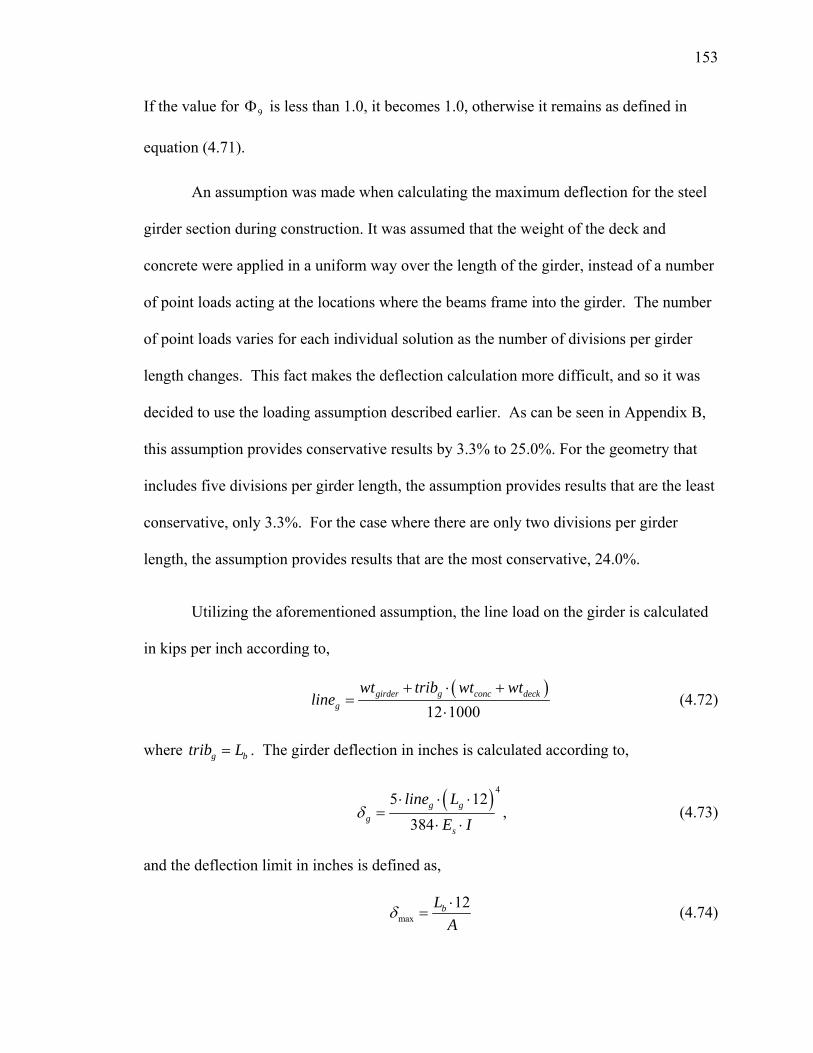
153
If the value for 9Φ is less than 1.0, it becomes 1.0, otherwise it remains as defined in
equation (4.71).
An assumption was made when calculating the maximum deflection for the steel
girder section during construction. It was assumed that the weight of the deck and
concrete were applied in a uniform way over the length of the girder, instead of a number
of point loads acting at the locations where the beams frame into the girder. The number
of point loads varies for each individual solution as the number of divisions per girder
length changes. This fact makes the deflection calculation more difficult, and so it was
decided to use the loading assumption described earlier. As can be seen in Appendix B,
this assumption provides conservative results by 3.3% to 25.0%. For the geometry that
includes five divisions per girder length, the assumption provides results that are the least
conservative, only 3.3%. For the case where there are only two divisions per girder
length, the assumption provides results that are the most conservative, 24.0%.
Utilizing the aforementioned assumption, the line load on the girder is calculated
in kips per inch according to,
( )
12 1000girder g conc deck
g
wt trib wt wtline
+ ⋅ +=
⋅ (4.72)
where g btrib L= . The girder deflection in inches is calculated according to,
( ) 4
5 12384
g gg
s
line LE I
δ⋅ ⋅ ⋅
=⋅ ⋅
, (4.73)
and the deflection limit in inches is defined as,
max12bL
Aδ ⋅
= (4.74)
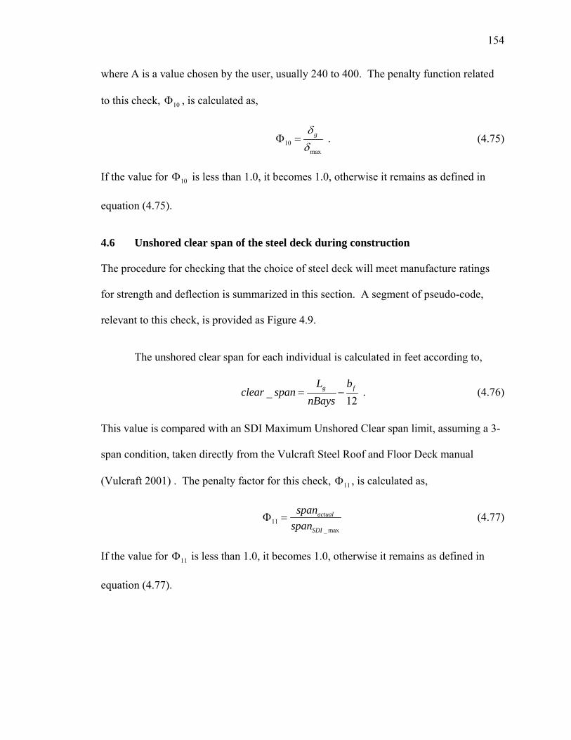
154
where A is a value chosen by the user, usually 240 to 400. The penalty function related
to this check, 10Φ , is calculated as,
10max
gδδ
Φ = . (4.75)
If the value for 10Φ is less than 1.0, it becomes 1.0, otherwise it remains as defined in
equation (4.75).
4.6 Unshored clear span of the steel deck during construction
The procedure for checking that the choice of steel deck will meet manufacture ratings
for strength and deflection is summarized in this section. A segment of pseudo-code,
relevant to this check, is provided as Figure 4.9.
The unshored clear span for each individual is calculated in feet according to,
_12
g fL bclear span
nBays= − . (4.76)
This value is compared with an SDI Maximum Unshored Clear span limit, assuming a 3-
span condition, taken directly from the Vulcraft Steel Roof and Floor Deck manual
(Vulcraft 2001) . The penalty factor for this check, 11Φ , is calculated as,
11_ max
actual
SDI
spanspan
Φ = (4.77)
If the value for 11Φ is less than 1.0, it becomes 1.0, otherwise it remains as defined in
equation (4.77).
155
4.7 Steel deck live load rating
The procedure for checking to determine if the applied superimposed live load is less
than the maximum allowable live load for a given deck gage and span is now reviewed.
The segments of pseudo-code relevant to this check have been provided in Figure 4.10.
The actual live load to be used in the program is established by the user as a part of the
array, sysIn, in the function master. The superimposed live load limit for each individual
solution is taken from the array allProps, which was established in the
function decodeChromo. The actual live load limit values were obtained from one of the
four EXCEL deck and slab files, which reflect data copied directly from the Vulcraft
Steel Roof and Floor Deck manual (Vulcraft 2001). The EXCEL files reflect a
condensed and reorganized form of the Vulcraft data that facilitates quick referencing by
the functions of the genetic algorithm. For more information on this process, see Section
3.3.
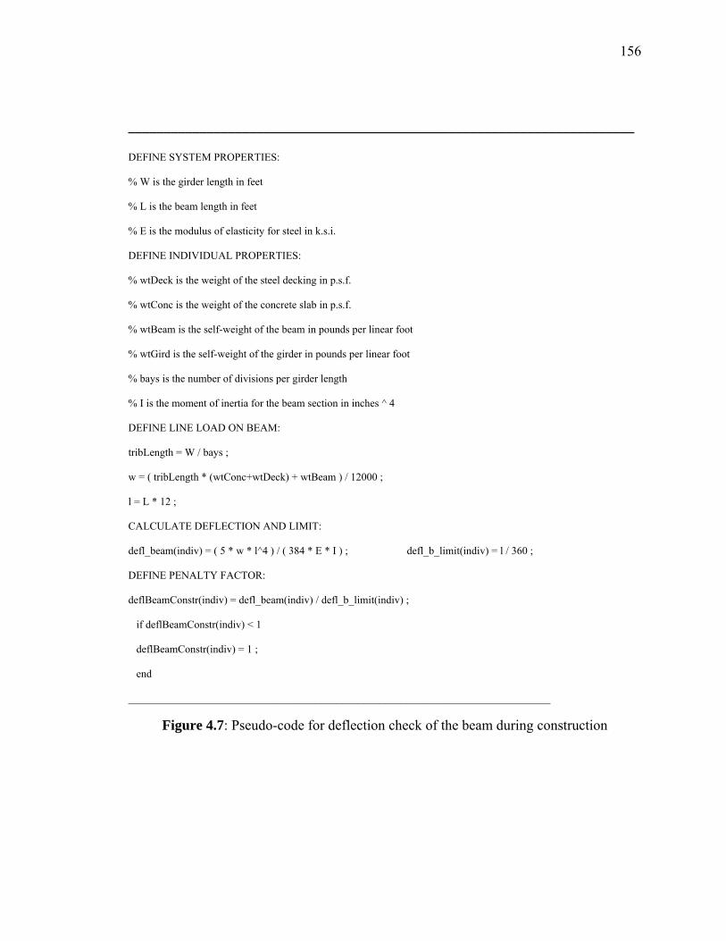
156
_______________________________________________________________________
DEFINE SYSTEM PROPERTIES:
% W is the girder length in feet
% L is the beam length in feet
% E is the modulus of elasticity for steel in k.s.i.
DEFINE INDIVIDUAL PROPERTIES:
% wtDeck is the weight of the steel decking in p.s.f.
% wtConc is the weight of the concrete slab in p.s.f.
% wtBeam is the self-weight of the beam in pounds per linear foot
% wtGird is the self-weight of the girder in pounds per linear foot
% bays is the number of divisions per girder length
% I is the moment of inertia for the beam section in inches ^ 4
DEFINE LINE LOAD ON BEAM:
tribLength = W / bays ;
w = ( tribLength * (wtConc+wtDeck) + wtBeam ) / 12000 ;
l = L * 12 ;
CALCULATE DEFLECTION AND LIMIT:
defl_beam(indiv) = ( 5 * w * l^4 ) / ( 384 * E * I ) ; defl_b_limit(indiv) = l / 360 ;
DEFINE PENALTY FACTOR:
deflBeamConstr(indiv) = defl_beam(indiv) / defl_b_limit(indiv) ;
if deflBeamConstr(indiv) < 1
deflBeamConstr(indiv) = 1 ;
end
_______________________________________________________________________________
Figure 4.7: Pseudo-code for deflection check of the beam during construction
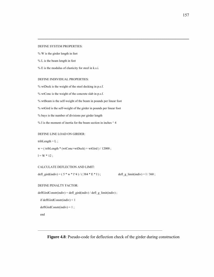
157
________________________________________________________________________
DEFINE SYSTEM PROPERTIES:
% W is the girder length in feet
% L is the beam length in feet
% E is the modulus of elasticity for steel in k.s.i.
DEFINE INDIVIDUAL PROPERTIES:
% wtDeck is the weight of the steel decking in p.s.f.
% wtConc is the weight of the concrete slab in p.s.f.
% wtBeam is the self-weight of the beam in pounds per linear foot
% wtGird is the self-weight of the girder in pounds per linear foot
% bays is the number of divisions per girder length
% I is the moment of inertia for the beam section in inches ^ 4
DEFINE LINE LOAD ON GIRDER:
tribLength = L ;
w = ( tribLength * (wtConc+wtDeck) + wtGird ) / 12000 ;
l = W * 12 ;
CALCULATE DEFLECTION AND LIMIT:
defl_gird(indiv) = ( 5 * w * l^4 ) / ( 384 * E * I ) ; defl_g_limit(indiv) = l / 360 ;
DEFINE PENALTY FACTOR:
deflGirdConstr(indiv) = defl_gird(indiv) / defl_g_limit(indiv) ;
if deflGirdConstr(indiv) < 1
deflGirdConstr(indiv) = 1 ;
end
_______________________________________________________________________________
Figure 4.8: Pseudo-code for deflection check of the girder during construction
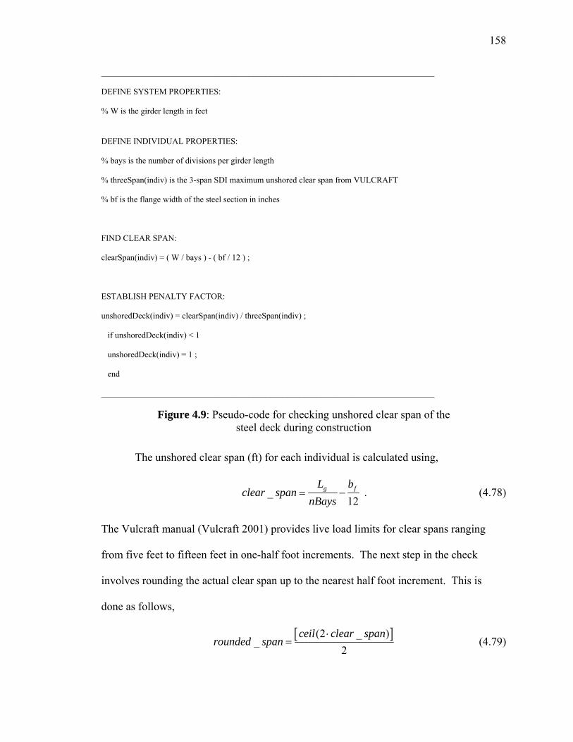
158
_______________________________________________________________________________
DEFINE SYSTEM PROPERTIES:
% W is the girder length in feet
DEFINE INDIVIDUAL PROPERTIES:
% bays is the number of divisions per girder length
% threeSpan(indiv) is the 3-span SDI maximum unshored clear span from VULCRAFT
% bf is the flange width of the steel section in inches
FIND CLEAR SPAN:
clearSpan(indiv) = ( W / bays ) - ( bf / 12 ) ;
ESTABLISH PENALTY FACTOR:
unshoredDeck(indiv) = clearSpan(indiv) / threeSpan(indiv) ;
if unshoredDeck(indiv) < 1
unshoredDeck(indiv) = 1 ;
end
_______________________________________________________________________________
Figure 4.9: Pseudo-code for checking unshored clear span of the steel deck during construction
The unshored clear span (ft) for each individual is calculated using,
_12
g fL bclear span
nBays= − . (4.78)
The Vulcraft manual (Vulcraft 2001) provides live load limits for clear spans ranging
from five feet to fifteen feet in one-half foot increments. The next step in the check
involves rounding the actual clear span up to the nearest half foot increment. This is
done as follows,
[ ](2 _ )_
2ceil clear span
rounded span⋅
= (4.79)
159
where ceil is a built-in MATLAB operator that rounds up to the next integer value.
Next, the live load limit will be located within the array allProps. The first 30
columns in the array allProps are for girder and beam properties. The next 14 columns in
allProps are for the deck and slab properties. The live load limits begin in the 45th
column. A marker (or pointer) is used to locate the correct column for the given rounded
clear span as,
2 ( _ 5) 45MARKER clear span= ⋅ − + (4.80)
which would reference the five foot clear span as being in the 45th column as described
above. The appropriate live load limit is then taken from the array allProps.
A check is next made to avoid a possible “divide by zero” error later in the
function. If the given deck series was does not include a clear span considered in the
system considered, the value for the live load limit will be zero. In the establishment of
the penalty function, later in this section, the penalty equals given live load divided by
live load limit, and a “divide by zero” error would result. To solve this problem, a check
is made to determine if the live load limit is zero. If it is zero, the value is altered to one.
This eliminates the possible error without affecting any later results.

160
_______________________________________________________________________________
DEFINE SYSTEM PROPERTIES:
% W is the girder length in feet
% actual_LL(indiv) is the live load establishes in master.m
DEFINE INDIVIDUAL PROPERTIES:
% bays is the number of divisions per girder length
% bf is the flange width of the steel section in inches
FIND CLEAR SPAN:
clearSpan = ( W / bays ) - ( bf / 12 ) ;
ROUND UP TO NEAREST HALF-FOOT:
clearSpan = ( ceil ( 2 * clearSpan ) ) / 2 ;
LOCATE LL RATING IN VULCRAFT TABLE:
marker = 2 * ( clearSpan - 5 ) + 45 ;
LL_limit(indiv) = allProps(indiv,marker) ;
TAKE CARE OF POSSIBLE DIVIDE BY ZERO CASE:
if LL_limit(indiv) == 0
LL_limit(indiv) = 1 ;
end
ESTABLISH PENALTY FUNCTION:
ratingDeck(indiv) = actual_LL(indiv) / LL_limit(indiv) ;
if ratingDeck(indiv) < 1
ratingDeck(indiv) = 1 ;
end
_______________________________________________________________________________
Figure 4.10: Pseudo-code for steel deck live load check
161
The penalty factor, 12Φ , is computed in the same manner as that previously
described. For the present constraint, we have,
12actual
LIMIT
LLLL
Φ = (4.81)
If the value for 12Φ is less than 1.0, it becomes 1.0, otherwise it remains as defined in
equation (4.81).
4.8 Floor panel acceleration due to walking excitation
An optional thirteenth check is used when non-dimensional acceleration limits are
desired in the evolution. In this case, a single-objective fitness statement is used, but
floor panel acceleration multipliers are applied. Pseudo-code for this check is shown in
Figure 4.11. The check is very simple because acceleration values are calculated with the
function floorVib, so no new calculations are required. The acceleration values are
compared against a recommended limit (AISC 1997), and the penalty factor, 13Φ , is
calculated as,
indiv
13
limit
p
p
agag
Φ = (4.82)
If the value for 13Φ is less than 1.0, it becomes 1.0, otherwise it remains as defined in
equation (4.82).
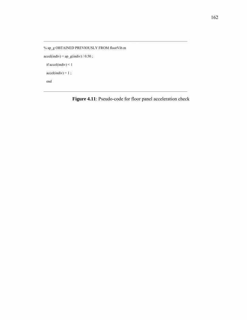
162
_______________________________________________________________________________
% ap_g OBTAINED PREVIOUSLY FROM floorVib.m
accel(indiv) = ap_g(indiv) / 0.50 ;
if accel(indiv) < 1
accel(indiv) = 1 ;
end
_______________________________________________________________________________
Figure 4.11: Pseudo-code for floor panel acceleration check

163
Chapter 5
Parameter Studies and Algorithm Performance
Six design examples will be analyzed in this chapter. They illustrate the results of varying
cost data, varying floor panel geometry, and altering the form of the fitness statement.
Except when noted, all examples will follow the floor panel layout used by Laman
(1999). This system has 30 'gL = , 40 'bL = , uses self-weight of the structure as the dead
load, includes 5 psf superimposed dead load, and uses 75 psf as the live load value.
The six design examples have been used to conduct five studies. Details
regarding the five studies will now be presented. The first study examines the sensitivity
of the design to steel fabrication costs and concrete costs. A base design is conducted
using accurate cost data obtained from local fabricators and contractors. The second
study evaluates the sensitivity of the design to panel dimension ratios using three panel
arrangements. The third study was used to test the performance of the algorithm.
Finally, the solutions obtained using a multiple objection formulation were evaluated.
Each study is discussed in detail in the following sections.
5.1 Sensitivity to Fabrication and Concrete Costs
A base design was first produced using realistic cost data. System information describing
the floor panel geometry and loading conditions for this design as well as the important
GA parameters is included in Table 5.1. Unit costs for the study in this section, as well
as the other studies in this chapter, are included in Table 5.2.

164
UNIT COSTS Sections 5.2, 5.3, 5.4
raw steel ($/lb.) 0.50 0.50 0.50 0.50
steel fab. ($/lb.) 0.50 1.00 0.50 0.50
deck ($/lb.) 1.00 1.00 1.00 1.00
NW conc. ($/yd3) 75.00 75.00 150.00 75.00
LW conc. ($/yd3) 85.00 85.00 170.00 85.00
shear stud ($) 4.50 9.00 4.50 4.50
TABLE 5.2: Unit Costs Associated with the Studies of Chapter 5
Section 5.1 (Base, 2*Fab., 2*Conc.)
Ten runs, or evolutions, of the genetic algorithm were made for the base design, as well
as the other design examples in this chapter. The best solution from each of the ten GA
evolutions of the base design is shown in Table 5.3.
Next, costs relating to steel fabrication were doubled. Shear stud installation was
considered to be steel fabrication, and so, stud cost was doubled also. The designs
resulting from these modified fabrication costs are included in Table 5.4. For the third
TABLE 5.1: System information for Sections 5.1, 5.3, 5.4
System to be analyzed, based on (Laman 1999) example:
W (girder length) in feet: 30 L (beam length) in feet: 40 Design DL in psf (not including self-weight): 5 Design LL in psf: 75 Desired number of generations: 35 Cut point for 75-per./25-per. scheme (0 to 100): 30 Mutation probability (0 to 1): 0.015 % of parents allowed to proceed to next gen.: 15 Population size: 250
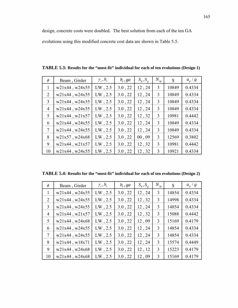
165
design, concrete costs were doubled. The best solution from each of the ten GA
evolutions using this modified concrete cost data are shown in Table 5.5.
TABLE 5.3: Results for the “most-fit” individual for each of ten evolutions (Design 1)
# Beam , Girder $1 w21x44 , w24x55 LW , 2.5 3.0 , 22 12 , 24 3 10849 0.43342 w21x44 , w24x55 LW , 2.5 3.0 , 22 12 , 24 3 10849 0.43343 w21x44 , w24x55 LW , 2.5 3.0 , 22 12 , 24 3 10849 0.43344 w21x44 , w24x55 LW , 2.5 3.0 , 22 12 , 24 3 10849 0.43345 w21x44 , w21x57 LW , 2.5 3.0 , 22 12 , 32 3 10981 0.44426 w21x44 , w24x55 LW , 2.5 3.0 , 22 12 , 24 3 10849 0.43347 w21x44 , w24x55 LW , 2.5 3.0 , 22 12 , 24 3 10849 0.43348 w21x57 , w24x68 LW , 2.5 3.0 , 22 00 , 09 3 12569 0.38029 w21x44 , w21x57 LW , 2.5 3.0 , 22 12 , 32 3 10981 0.4442
10 w21x44 , w24x55 LW , 2.5 3.0 , 22 12 , 32 3 10921 0.4334
,c chγ ,rh ga ,b gS S spN /pa g
TABLE 5.4: Results for the “most-fit” individual for each of ten evolutions (Design 2)
# Beam , Girder $1 w21x44 , w24x55 LW , 2.5 3.0 , 22 12 , 24 3 14854 0.43342 w21x44 , w24x55 LW , 2.5 3.0 , 22 12 , 32 3 14998 0.43343 w21x44 , w24x55 LW , 2.5 3.0 , 22 12 , 24 3 14854 0.43344 w21x44 , w21x57 LW , 2.5 3.0 , 22 12 , 32 3 15088 0.44425 w21x44 , w24x68 LW , 2.5 3.0 , 22 12 , 09 3 15169 0.41796 w21x44 , w24x55 LW , 2.5 3.0 , 22 12 , 24 3 14854 0.43347 w21x44 , w24x55 LW , 2.5 3.0 , 22 12 , 24 3 14854 0.43348 w21x44 , w18x71 LW , 2.5 3.0 , 22 12 , 24 3 15574 0.44499 w21x44 , w24x68 LW , 2.5 3.0 , 22 12 , 12 3 15223 0.4179
10 w21x44 , w24x68 LW , 2.5 3.0 , 22 12 , 09 3 15169 0.4179
,c chγ ,rh ga ,b gS S spN /pa g

166
TABLE 5.5: Results for the “most-fit” individual for each of ten evolutions (Design 3) y
# Beam , Girder $1 w21x44 , w24x55 NW , 2.5 3.0 , 21 12 , 24 3 12077 0.36512 w21x44 , w24x68 NW , 2.5 3.0 , 21 12 , 12 3 12330 0.35123 w21x44 , w24x68 NW , 2.5 3.0 , 21 12 , 12 3 12330 0.35124 w21x44 , w21x57 LW , 2.5 3.0 , 22 12 , 32 3 12235 0.44425 w21x44 , w24x68 NW , 2.5 3.0 , 21 12 , 12 3 12330 0.35126 w21x44 , w21x57 LW , 2.5 3.0 , 22 12 , 32 3 12235 0.44427 w18x35 , w24x62 NW , 2.5 1.5 , 21 12 , 20 4 12130 0.49038 w21x44 , w21x57 LW , 2.5 3.0 , 22 12 , 28 3 12304 0.44429 w21x44 , w24x55 NW , 2.5 3.0 , 21 12 , 24 3 12077 0.3651
10 w21x44 , w21x57 LW , 2.5 3.0 , 22 12 , 32 3 12235 0.4442
,c chγ ,rh ga ,b gS S spN /pa g
The results for the least-cost individual from the base design are identical to the
results for the least-cost solution in the modified fabrication design. The only difference
is the total cost, which was expected to change because of higher unit costs for
fabrication. Both solutions used w21x44 beams with w24x55 girders with 2.5-inches of
light-weight concrete over a 3.0-inch, 22-gage deck. Both solutions used 12 beam studs
and 24 girder studs per half span and had the panel divided into 3 bay spacings. Based on
these results, it would seem that the genetic algorithm designs are insensitive to moderate
increases in steel fabrication costs.
The results for the least-cost individual from the design with modified concrete
costs are very similar to the results from the base design. The only difference is that the
individual from the modified concrete costs design uses normal-weight concrete instead
of light-weight concrete and uses a deck that is slightly thicker. These results seem to
make sense, because the normal-weight concrete is less expensive, especially when costs
are doubled. Also, the normal-weight concrete increases the weight of the floor slab, and

167
so it seems logical that a thicker deck might be required. Based on these results, a
conclusion is drawn that moderate increases in concrete costs may have a slight impact
on the most economical design. The increased costs will often lead to the use of normal-
weight concrete with a slightly thicker deck.
5.2 Sensitivity to Floor Panel Dimensions
Study 2 was used to evaluate the effects of different floor panel configurations on the
characteristics of the least-cost solution. Three systems were analyzed with different
values for the ratio of beam length to girder length, b
g
LL
. The first system used an b
g
LL
ratio of 43
. The beam length, bL , was equal to 40-feet while the girder length, gL , was
equal to 30-feet. Results for the most-fit individual for each of the ten evolutions are
included in Table 5.3. The second and third systems, with b
g
LL
ratios of 1 and 34
,
respectively, have dimensions that are described in Table 5.6. Results for the most-fit
individuals for systems 2 and 3, are included in Tables 5.7 and 5.8, respectively.
The results of Study 2 illustrate that different types of solutions will be produced
by the GA for changes in the ratio of b
g
LL
. For an b
g
LL
ratio of 43
, the least-cost solution
used 3spN = . For an b
g
LL
ratio of 1.0, the least-cost solution used 5spN = . And for an
b
g
LL
ratio of 34
, the least-cost solution used 4spN = .

168
These results make sense in some ways and no sense in other ways. For the
system with 40-feet and = 30-feetb gL L= , it has been seen previously that the least-cost
solution will often use 3spN = , and so this result makes sense. But, as the girder length,
gL , increases to 40-feet, a change to perhaps 4spN = would be expected, but a change to
5spN = was seen. This change seems to be too extreme given a moderate change in the
girder length. However, the results of Table 5.7 show that eight of the ten other least-
cost solutions used 4spN = , which makes sense.
TABLE 5.6: Alternate Floor Panel Configurations for Section 5.2
Design 4:
System to be analyzed:
W (girder length) in feet: 40 L (beam length) in feet: 40 Design DL in psf (not including self-weight): 5 Design LL in psf: 75 Desired number of generations: 35 Cut point for 75-per./25-per. scheme (0 to 100): 30 Mutation probability (0 to 1): 0.015 % of parents allowed to proceed to next gen.: 15 Population size: 250
Design 5:
System to be analyzed:
W (girder length) in feet: 40 L (beam length) in feet: 30 Design DL in psf (not including self-weight): 5 Design LL in psf: 75 Desired number of generations: 35 Cut point for 75-per./25-per. scheme (0 to 100): 30 Mutation probability (0 to 1): 0.015 % of parents allowed to proceed to next gen.: 15 Population size: 250
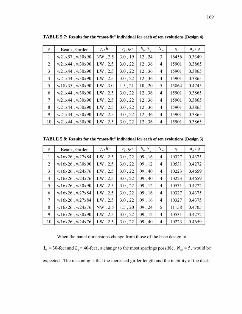
169
TABLE 5.7: Results for the “most-fit” individual for each of ten evolutions (Design 4)
# Beam , Girder $1 w21x57 , w30x90 NW , 2.5 3.0 , 19 12 , 24 3 16456 0.33492 w21x44 , w30x90 LW , 2.5 3.0 , 22 12 , 36 4 15901 0.38653 w21x44 , w30x90 LW , 2.5 3.0 , 22 12 , 36 4 15901 0.38654 w21x44 , w30x90 LW , 2.5 3.0 , 22 12 , 36 4 15901 0.38655 w18x35 , w30x90 LW , 3.0 1.5 , 21 10 , 20 5 15864 0.47456 w21x44 , w30x90 LW , 2.5 3.0 , 22 12 , 36 4 15901 0.38657 w21x44 , w30x90 LW , 2.5 3.0 , 22 12 , 36 4 15901 0.38658 w21x44 , w30x90 LW , 2.5 3.0 , 22 12 , 36 4 15901 0.38659 w21x44 , w30x90 LW , 2.5 3.0 , 22 12 , 36 4 15901 0.3865
10 w21x44 , w30x90 LW , 2.5 3.0 , 22 12 , 36 4 15901 0.3865
,c chγ ,rh ga ,b gS S spN /pa g
TABLE 5.8: Results for the “most-fit” individual for each of ten evolutions (Design 5)
# Beam , Girder $1 w16x26 , w27x84 LW , 2.5 3.0 , 22 09 , 16 4 10327 0.43752 w16x26 , w30x90 LW , 2.5 3.0 , 22 09 , 12 4 10531 0.42723 w16x26 , w24x76 LW , 2.5 3.0 , 22 09 , 40 4 10223 0.46594 w16x26 , w24x76 LW , 2.5 3.0 , 22 09 , 40 4 10223 0.46595 w16x26 , w30x90 LW , 2.5 3.0 , 22 09 , 12 4 10531 0.42726 w16x26 , w27x84 LW , 2.5 3.0 , 22 09 , 16 4 10327 0.43757 w16x26 , w27x84 LW , 2.5 3.0 , 22 09 , 16 4 10327 0.43758 w16x26 , w24x76 NW , 2.5 1.5 , 20 09 , 24 5 11158 0.47059 w16x26 , w30x90 LW , 2.5 3.0 , 22 09 , 12 4 10531 0.4272
10 w16x26 , w24x76 LW , 2.5 3.0 , 22 09 , 40 4 10223 0.4659
,c chγ ,rh ga ,b gS S spN /pa g
When the panel dimensions change from those of the base design to
30-feet and = 40-feetb gL L= , a change to the most spacings possible, 5spN = , would be
expected. The reasoning is that the increased girder length and the inability of the deck

170
to span large distances would require that the maximum number of spacings be used.
However, a change to only 4spN = was seen.
This behavior could be explained, possibly, using the following reasoning. When
the panel dimensions are changed to 30-feetbL = and = 40-feetgL , the girder width has
increased by 10-feet, so more spacings would be expected. A spacing of perhaps 5 would
seem reasonable. But, with the beam span at 75% of its previous length, the moment
capacity required is now at (75%)2 = 56.3% of the previous amount, according to
equation (5.1).
2
8uwLM = (5.1)
So, the need for more beam spacings because of the increased girder length is offset by
the reduced strength capacity required of the beams, and a value like 4spN = seems to
make sense.
Another comparison is made between the least-cost solution of Design 1 and the
least-cost solution of Design 5. These two designs illustrate the results of switching the
direction in which the beams and girders run. Panel costs for the least-cost individual
from each design are very similar. For Design 1, the least-cost individual had a cost of
$10,849. For Design 5, the least-cost individual had a cost of $10,223. Based on these
results, it would appear that there is no “preferred” girder direction.

171
5.3 Algorithm Performance
Study 3 has been used to evaluate the performance of the genetic algorithm. GA traits
such as stability, reliability, and convergence speed have been examined. The results
from Design 1 shown in Table 5.3 were used for the analysis.
The least-cost solution for this design occurred as the best solution for six of the
ten evolutions. These six solutions are identical with respect to all nine characteristics.
The other four solutions are very similar, with one small change in the beam section
(from w21x44 to w21x57) and three slight changes in the girder section (from w24x55 to
w21x57 or w24x68). Cost variance with respect to the least-cost solution ranged from
0.67% for solution #10 to 15.8% for solution #8. All ten solutions use light-weight
concrete with a slab thickness, ch , equal to 2.5-inches. All ten solutions also use a 3.0
VLI deck series with a 22-gage thickness. The value for beam studs varied from 0 to 12
per half span, while the value for girder studs varied from 9 to 32 per half span. All
solutions used 3spN = .
A convergence trajectory plot has been included in Figure 5.9. The plot shows
the cost of the most-fit individual for each of the 35 generations for each of the ten
evolutions. The plot demonstrates how rapidly the solutions progress towards
convergence, even within the first five generations. It can also be seen that all but one
solution (#8) end up with least-cost values in the same range.

172
The results of the GA prove that it is robust. The fact that the GA was able to
reproduce the least-cost solution six times, when starting with a population of individuals
with randomly chosen characteristics, shows that the GA is stable. Its designs have been
checked for strength, deflection, and vibration performance accuracy against hand
calculations, demonstrating reliability.
As a way to evaluate whether the GA solutions truly represent optimal solutions,
one would have to do an exhaustive search, evaluating all possible combinations, until
the single best solution is found. With the given material choices, there are,
0 5 10 15 20 25 30 351
1.1
1.2
1.3
1.4
1.5
1.6
1.7
1.8
1.9x 10
4
Generation
Cost
for
"fitt
est
" in
div
idual
Convergence Trajectory Plot, MATLAB GA
Figure 5.9: Convergence Trajectory Plot For Design 1
173
2 2& & & &256 8 8 4 32beam girder conc type thickness deck height gage bayconfig beam girder stud⋅ ⋅ ⋅ ⋅
which equals 17.2 billion combinations. A computer program would be required to make
this number of fitness evaluations. This process would be lengthy, even with a powerful
computer. Knowing that a single GA run takes around eight minutes, and conservatively
estimating that the GA expends 90% of its computing resources on genetic algorithm-
related tasks, it would take 109 days to simply evaluate the fitness of all 17.2 billion
combinations.
It is easy to see why the GA-based search is so useful. To produce its best
solution, the GA has to deal with,
250 35 10individuals generations evolutions⋅ ⋅
which equals only 87,500 fitness evaluations. Based on
this information, the benefit of using the GA is apparent.
5.4 Multiple Objective Optimization
In study 4, the maximin fitness function was used to evaluate the fitness of each solution
based on two objectives. The two objectives were total floor panel cost and
dimensionless acceleration due to walking excitation. More information regarding the
method used to assign fitness based on these two objectives can be found in Section 3.11.
Study 4 uses the same (Laman 1999) system information describing the floor panel
geometry and loading conditions as the other studies. All GA parameters were the same
as used previously, except that this design ran a single evolution using 40 generations.
Progress of the genetic algorithm through a single evolution is demonstrated by
the plots in Figures 5.10 to 5.12. The two plots in Figure 5.10 show the 125 most-fit

174
solutions for a population of 250 at the end of the first and tenth generations,
respectively. The data used is that of Design 6. Similarly, the two plots in Figure 5.11
show the 125 most-fit solutions at the end of the twentieth and thirtieth generations,
respectively. The plot in Figure 5.12 shows the 125 most-fit solutions at the end of the
fortieth generation.
Two solutions are labeled on the plot of Figure 5.12 as Solutions 5A and 5B.
Solution 5A is the least-cost solution with a higher acceleration value. It makes use of
w44x230 beams and w44x335 girders with 4 inches of normal-weight concrete over a
3.0-inch, 20-gage deck. Solution 5A uses 3 beam spacings with 0 shear studs per half
beam and 20 shear studs per half girder. Solution 5B is the most expensive solution with
the lowest acceleration value. It makes use of w44x335 beams and w40x593 girders with
4 inches of normal-weight concrete over a 3.0-inch, 20-gage deck. Solution 5B uses 3
beam spacings with 72 shear studs per half beam and 36 shear studs per half girder.
This study demonstrates some of the positive and negative features of the
maximin fitness method. The method did lead the genetic algorithm to a final generation
that is “...both close to the universal Pareto front and diverse,” as indicated in Balling et
al. (2001). The maximin function did operate the way it was designed to, but it was not
effective in the context of this floor framing problem. Using this fitness function, equal
emphasis was placed on minimizing both cost and acceleration performance. This results
in solutions that are very sturdy with very low dimensionless acceleration values. The
trade-off is that these solutions cost 2 to 3 times as much as least-cost solutions from
Study 1.
175
The maximin fitness function tries to minimize acceleration, when all that is
really needed is to keep acceleration values below the 0.5000% limit. The maximin
fitness function would be useful for building designers who were seeking to create a
building with ultra-low vibrations. This type of structure might house sensitive
equipment, like the equipment found in a robotic surgery suite within a hospital. In this
case, solutions with good vibration performance are produced by the GA at a minimum
cost increase.
5.5 General Observations and Concluding Remarks
Based on the results of Design 1, where realistic cost data was used, common traits for
the least-cost solutions have been observed. Using light-weight concrete often leads to
most economical framing systems, as does using fewer panel divisions. Also, using the
taller, 3.0-inch deck in a thinner gage leads to solutions with a lower total cost.
The results of Study 1 show that moderate cost increases relating to steel
fabrication have little to no effect on the most economical solution. This would imply
that the best design is independent of steel fabrication costs. The results also show that
moderate cost increases relating to concrete costs have a slight impact on the most-
economical framing system. These cost increases often lead to the use of normal-weight
concrete with a slightly thicker steel deck.
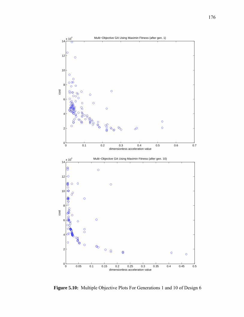
176
0 0.1 0.2 0.3 0.4 0.5 0.6 0.70
2
4
6
8
10
12
14x 10
4
dimensionless acceleration value
cost
Multi−Objective GA Using Maximin Fitness (after gen. 1)
0 0.05 0.1 0.15 0.2 0.25 0.3 0.35 0.4 0.45 0.50
2
4
6
8
10
12
14x 10
4
dimensionless acceleration value
cost
Multi−Objective GA Using Maximin Fitness (after gen. 10)
Figure 5.10: Multiple Objective Plots For Generations 1 and 10 of Design 6
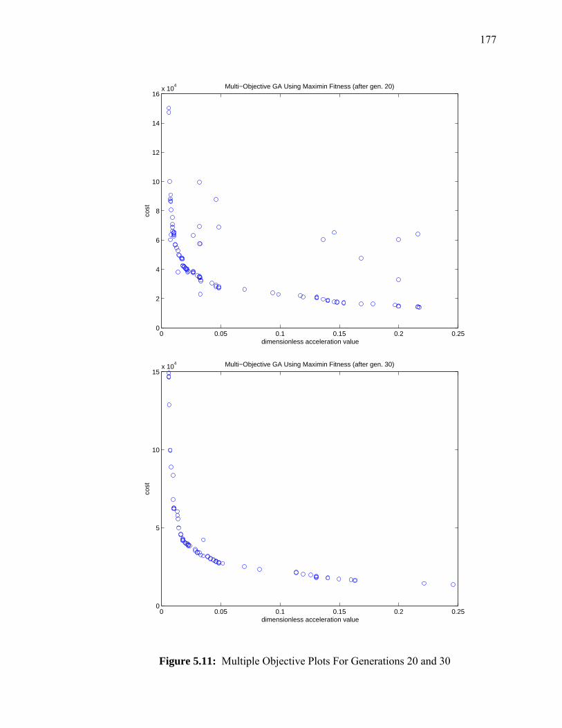
177
0 0.05 0.1 0.15 0.2 0.250
2
4
6
8
10
12
14
16x 10
4
dimensionless acceleration value
cost
Multi−Objective GA Using Maximin Fitness (after gen. 20)
0 0.05 0.1 0.15 0.2 0.250
5
10
15x 10
4
dimensionless acceleration value
cost
Multi−Objective GA Using Maximin Fitness (after gen. 30)
Figure 5.11: Multiple Objective Plots For Generations 20 and 30

178
The results of Study 1 also illustrate the effects of concrete choice on the
acceleration performance of the floor system when subjected to walking excitation.
It can be seen in Tables 5.3 to 5.5 that the use of light-weight concrete leads to higher
values for the dimensionless acceleration value, pag
. The least-cost solution from the
base design, using light-weight concrete, has an pag
value of 0.4334% when the
recommended limit is 0.5000%. The similar solution, from the design with concrete
0 0.02 0.04 0.06 0.08 0.1 0.12 0.14 0.16 0.18 0.21.5
2
2.5
3
3.5
4
4.5
5
5.5
6
6.5x 10
4
dimensionless acceleration value
cost
Multi−Objective GA Using Maximin Fitness (after gen. 40)
Figure 5.12: Multiple Objective Plot For Final Generation
Solution 5A
Solution 5B
179
costs doubled, uses normal-weight concrete and a slightly thicker deck, and has an pag
value of 0.3651%. This observation can possibly be explained by the fact that the total
mass weight of the floor system, W, will be reduced when using light-weight concrete,
leading to larger values for pag
, defined as,
( 0.35 )nf
p oa P eg Wβ
− ⋅⋅=
⋅ (5.2)
If better acceleration performance is desired by a designer, normal-weight concrete
should be used.
The results of Study 1 also illustrate that different framing layouts can be
economical and effective within the same problem. Solution #7 in Table 5.5 has the floor
panel divided into four spacings instead of three. The 4spN = solution is only 0.44%
higher in price than the least-cost solution with 3spN = . The trade-off, however, is that
the change to four spacings leads to a much higher value for the dimensionless
acceleration value, pag
, but a value that is still within the limit of 0.5000%.
This relationship between more spacings and higher acceleration values is also
seen in Study 2. The results of Design 4 in Table 5.7 show that although solution 5 is the
least-cost solution, it uses 5spN = and has an pag
value that is very close to the 0.5000%
limit. The next least-cost solution costs only 0.23% more, but it uses 4spN = and
performs significantly better in the acceleration evaluation. The third least-cost solution
180
costs only 3.7% more than the best solution, but uses 3spN = and performs better still in
terms of floor panel acceleration.
The explanation for this behavior seems to be connected with the equation used
for floor panel acceleration, shown previously as equation (5.2). The solutions with more
spacings seem to be lighter in terms of overall panel weight, leading to lower values for
the mass weight of the floor system, W, and higher values for the dimensionless
acceleration, pag
. These results lead to the conclusion that if designers are trying to
improve the floor panel acceleration performance, using fewer spacings is preferred.
Study 4 demonstrates that maximin fitness is not effective as a multi-objective
fitness operator in the context of this floor framing problem. The maximin method does
perform as designed, and does lead to a final generation of individuals that are both
diverse and along the universal Pareto front. However, the method is placing equal
emphasis on each of the two objectives, total panel cost and floor panel acceleration. For
most circumstances, it is not desired to minimize the floor panel accelerations, but rather
to simply keep them below an acceptable limit. The maximin fitness operator could
prove useful when designing structures to house ultra-sensitive equipment, like robotic
surgery suites, where very little vibration could be tolerated. In this case, the genetic
algorithm using maximin fitness would be the perfect way to achieve exceptional
vibration performance at a minimum cost.
A genetic algorithm-based program has been developed to provide optimal or
near-optimal solutions for a steel floor framing problem. Based on the input of system
181
geometry and loading conditions, the program produces details of the best solutions such
as the wide-flange sections used, deck and slab properties, shear connector
configurations, and floor panel layout information. The solutions provided by the genetic
algorithm have been studied, and have proven to be repeatable and reliable. The genetic
algorithm is robust, and is able to provide solutions to floor panel designs with various
geometries and loadings. The genetic algorithm could be used by designers, as well as
researchers, who wish to gain an understanding of the performance of steel floor panels
that are framed with wide-flanged sections.
182
Chapter 6
Recommendations for Future Research
A genetic algorithm-based program has been developed to design steel wide-flanged
floor systems based on strength, serviceability, and performance criteria. As input, it
requires only system geometry and loading conditions. After completing an evolution,
the program is able to supply details describing the best solutions. Some simple studies
have been completed as described in Chapter 5. However, there are many additional
studies that could be conducted. These studies, along with other ways in which the
performance and application of the GA could be improved, are listed below.
• Provide the program user with a graphical user interface (GUI). This would
allow the user to control both the floor panel geometry values and the genetic
algorithm parameters. Currently, all of these values are adjustable, but they
are hard coded within the function master.m.
• The program presented makes use of wide-flange sections only for beams and
girders. A fellow graduate student, Christopher Erwin, at Marquette
University, has prepared a similar genetic algorithm-based program to design
floor systems using open-web steel joists. The two programs could be
combined in order to explore the economics of using wide-flange beams as
opposed to open-web joists for specific building types, building uses, and
floor panel configurations.

183
• The cost of fireproofing for the steel structure could be examined. It would be
easy to calculate fireproofing costs based on the wide-flange members’
dimensions. The cost of fireproofing could then be added to the total panel
cost.
• More choices could be provided to the genetic algorithm in the areas of deck
and slab choices. The Vulcraft manual (Vulcraft 2001) provided data for a 2
VLI (2-inch rib height) deck series as well as a 1.5 VLR (1.5-inch rib height).
The 1.5 VLR deck series is similar to the 1.5 VLI that was used, but with
slightly different properties. Deck gages of 16, 17, and 18 are available in
addition to the 19, 20, 21, and 22 that were used for the GA. Added concrete
thicknesses were also provided for each deck series but not used within the
GA.
• The use of a more effective multi-objective fitness operator could be explored.
Maximin fitness (Balling et al. 2001) was implemented, and was operating
correctly, but proved not to be the best method for this problem. The maximin
fitness statement was not able to recognize that the two objectives were of
different importance, and tried to minimize both. Results showed that the
individuals that performed very well in the vibration objective were favored
over those individuals who had very low costs. For most applications of the
genetic algorithm to real framing problems, cost must be minimized while
simply keeping acceleration values below a specified limit.

184
• A series of design charts could be produced, providing building designers with
the most economical options for typical framing configurations. Trends
could be examined, relating certain framing systems with certain building use
categories.
• An attempt could be made to make the program run faster. Typical run times
for the single-objective version with a 250 population size, 35 generations,
and 10 repeat runs are around 7 to 8 minutes on a Pentium 4 CPU at 1.7 GHz.
Two methods could be used to reduce the run times. A more powerful
computer, or group of computers, could be utilized to run the program. Or, an
attempt could be made to make the GA more efficient, by eliminating or
reducing some of the large arrays that are being used by MATLAB.
Currently, much of the data is stored in large 2-D arrays. The program could
also be made to run faster by initializing each array with zeros before each
generation.
• Additional studies could be performed relating to GA parameters and floor
panel geometries. GA parameters like mutation probability, cut-point for
partitioning-based selection mechanism, and percentage for the elitism system
have been included in the GA, but have not been studied as to their
effectiveness at providing good solutions. The effect of different crossover
methods could also be studied. The effect of using different floor panel ratios,
equal to
b
g
LL , could also be further investigated. It could be determined that

185
certain ratios provide the most economical systems for certain building uses
and types.
• Studies could be performed on existing buildings with known vibration
problems as a result of walking excitation. The GA could be used to evaluate
what type of framing system might have provided better performance.
• Complete enumeration, or a systematic evaluation of all possible solutions to
an individual problem, could be used to evaluate the success of the GA. With
the given material choices, there are:
2 2& & & &256 8 8 4 32beam girder conc type thickness deck height gage bay config beam girder stud⋅ ⋅ ⋅ ⋅
which equals 17.2 billion required fitness evaluations. Knowing that a single
GA run takes around eight minutes, and conservatively estimating that the GA
expends 90% of its computing resources on genetic algorithm-related tasks, it
would take 109 days to simply evaluate the fitness of all 17.2 billion
combinations. It is easy to see why the GA-based search is so useful.
186
References AISC. (2001). LRFD Specification for Structural Steel Buildings, American Institute of
Steel Construction, Chicago, IL. Balling, R. J., and Wilson, S. (2001). “The Maximin Fitness Function for Multi-objective
Evolutionary Computation: Application to City Planning.” Evolutionary Design of Engineered Structures: Proceedings of the Genetic and Evolutionary Computation Conference, July 7-11, 2001, San Francisco, CA, 1079-1084.
Chien, E. Y. L., and Ritchie, J. K. (1993). “Composite floor systems – a mature design
option.” Journal of constructional Steel Research, Vol. 25, No. 1-2, 107-139. Coello Coello, C. A., Christiansen, A. D., and Hernandez, F. S. (1997). “A Simple
Genetic Algorithm for the Design of Reinforced Concrete Beams.” Engineering With Computers, 13: 185-196.
Coley, D. A. (1999). An Introduction to Genetic Algorithms for Scientists and Engineers,
World Scientific Publishing Co., River Edge, NJ. Goldberg, D. E. (1989). Genetic algorithms in search, optimization, and machine
learning. Addison-Wesley, Reading, Massachusetts. Hajela, P., Lee, E., and Cho, H. (1998). “Genetic Algorithms in Topologic Design of
Grillage Structures.” Computer-Aided Civil and Infrastructure Engineering, Vol. 13, No. 1, 13-22.
Haupt, R. L., and Haupt, S. E. (1998). Practical Genetic Algorithms, John Wiley and
Sons, Inc., New York, NY. Hayalioglu, M. S. (2001). “Optimum Load and Resistance Factor Design of Steel Space
Frames Using Genetic Algorithm.” Structural and Multidisciplinary Optimization: Journal of the International Society for Structural and Multidisciplinary Optimization, 21, 292-299.
Herniter, M. E. (2001). Programming in MATLAB, Brooks/Cole Publishers, Pacific
Grove, CA. Holland, J. H. (1975). “Adaptation in Natural and Artificial Systems.” University of
Michigan Press, Ann Arbor, MI. Huang, M. W., and Arora, J. S. (1997). “Optimal Design of Steel Structures Using
Standard Sections.” Structural Optimization, 14, 24-35.
187
Huang, M. W., and Arora, J. S. (1997). “Performance of a Genetic Algorithm For Structural Design Using Available Sections.” Building to Last Structures Congress: Proceedings, Vol. 2, 793-797.
Jain, D., Krawinkler, H., Law, K. H., and Luth, G. P. (1991). “Formal approach to
automating conceptual structural design, part II: application to floor framing generation.” Engineering with Computers, Vol. 7, No. 2, 91-107.
Kameshki, E. S., and Saka, M. P. (2001). “Optimum Design of Nonlinear Steel Frames
With Semi-rigid Connections Using a Genetic Algorithm.” Computers & Structures, Vol. 79, No. 17, 1593-1604.
Koumousis, V. K., and Georgiou, P. G. (1994). “Genetic Algorithms in Discrete
Optimization of Steel Truss Roofs.” Journal of Computing in Civil Engineering, Vol. 8, No. 3, 309-325.
Laman, Jeffrey A. (1999). “Design Aids for Walking Vibrations in Steel Framed Floors.”
Engineering Journal, Second Quarter, 1999, 82-101. Mathworks (2003). Developers of MATLAB and Simulink for Technical Computing.
http://www.mathworks.com, © 2003. Murray, T.M., Allen, D.E., and Ungar, E.E. (1997). AISC Steel Design Guide Series 11
Floor Vibrations Due to Human Activity, American Institute of Steel Construction, Chicago, IL.
Murray, T. M., Allan, D. E., Ungar, E. E. (1997). “Designing Steel for Serviceability
Lecture 5 Control of Floor Vibrations.” Murray, T. M., Allan, D. E. (1993). “Design Criterion for Vibrations Due to Walking.”
Engineering Journal, Fourth Quarter, 1993, 117-129. Murray, T. M. (1991). “Building Floor Vibrations.” 1991 National Steel Construction
Conference Proceedings Sponsored by the American Institute of Steel Construction, Washington, D.C., 19.1–19.18.
Pezeshk, S., Camp, C. V., and Chen, D. (1998). “Optimized Design of Two-dimensional
Structures Using a Genetic Algorithm.” Journal of Structural Engineering, Vol. 124, No. 5, 551-559.
Pezeshk, S., Camp, C. V., and Chen, D. (1999). “Genetic Algorithm for Design of
Nonlinear Framed Structures.” Structural Engineering in the 21st Century; Proceedings of the 1999 Structures Congress, April 18-21, 1999, New Orleans, LA, 498-501.
188
Pezeshk, S., Camp, C. V., and Chen, D. (2000). “Design of Nonlinear Framed Structures Using Genetic Optimization.” Journal of Structural Engineering, Vol. 126, No. 3, 382-388.
Pezeshk, S., and Camp, C. V. (2002). “Chapter 3: State of the Art on the Use of Genetic
Algorithms in Design of Steel Structures.” Recent Advances in Optimal Structural Design, 55-79.
Rajan, S. D., Mobasher, B., Chen, S. Y., and Young, C. (1999). “Cost-based Design of
Residential Steel Roof Systems: A Case Study.” Structural Engineering and Mechanics, Vol. 8, No. 2, 165-180.
Saka, M. P. (1998). “Optimum Design of Grillage Systems Using Genetic Algorithms.”
Computer-Aided Civil and Infrastructure Engineering, Vol. 13, No. 4, 297-302. Salmon, C. G., and Johnson, J. E. (1996). Steel Structures: Design and Behavior,
Emphasizing Load and Resistance Factor Design, HarperCollins College Publishers, New York, NY.
Sarma, K. C., and Adeli, H. (2000). “Fuzzy Genetic Algorithm for Optimization of Steel
Structures.” Journal of Structural Engineering, Vol. 126, No. 5, 596-604. Schinler, D. C. (2001). “Design of Partially Restrained Steel Frames Using Advanced
Analysis and an Object-Oriented Evolutionary Algorithm.” Master of Science Thesis, Marquette University, Milwaukee, WI.
Toropov, V. V., and Mahfouz, S. Y. (2001). “Design Optimization of Structural
Steelwork Using a Genetic Algorithm, FEM, and a system of design rules.” Engineering Computations, Vol.18, No. 3 of 4, 437-459.
Torregosa, R. F., and Kanok-Nukulchai, W. (2002). “Weight Optimization of Steel
Frames Using Genetic Algorithm.” Advances in Structural Engineering, Vol. 5, No. 2, 99-111.
Vulcraft, Nucor Corporation (2001). Steel Roof and Floor Deck, Nucor Corporation, St.
Joe, IN. Wang, C. K., and Salmon, C. G. (1998). Reinforced Concrete Design, Addison Wesley
Educational Publishers, Inc., New York, NY.

189
Appendix A – Full MATLAB Function Source Listings
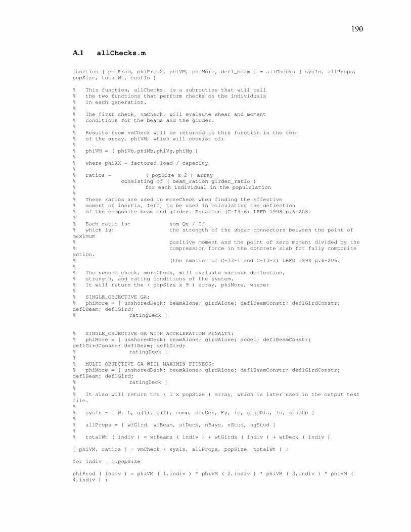
190
A.1 allChecks.m function [ phiProd, phiProd2, phiVM, phiMore, defl_beam ] = allChecks ( sysIn, allProps, popSize, totalWt, costIn ) % This function, allChecks, is a subroutine that will call % the two functions that perform checks on the individuals % in each generation. % % The first check, vmCheck, will evalaute shear and moment % conditions for the beams and the girder. % % Results from vmCheck will be returned to this function in the form % of the array, phiVM, which will consist of: % % phiVM = ( phiVb,phiMb,phiVg,phiMg ) % % where phiXX = factored load / capacity % % ratios = ( popSize x 2 ) array % consisting of ( beam_ration girder_ratio ) % for each individual in the popululation % % These ratios are used in moreCheck when finding the effective % moment of inertia, Ieff, to be used in calculating the deflection % of the composite beam and girder. Equation (C-I3-6) LRFD 1998 p.6-208. % % Each ratio is: sum Qn / Cf % which is: the strength of the shear connectors between the point of maximum % positive moment and the point of zero moment divided by the % compression force in the concrete slab for fully composite action. % (the smaller of C-I3-1 and C-I3-2) LRFD 1998 p.6-206. % % The second check, moreCheck, will evaluate various deflection, % strength, and rating conditions of the system. % It will return the ( popSize x 9 ) array, phiMore, where: % % SINGLE_OBJECTIVE GA: % phiMore = [ unshoredDeck; beamAlone; girdAlone; deflBeamConstr; deflGirdConstr; deflBeam; deflGird; % ratingDeck ] % SINGLE_OBJECTIVE GA WITH ACCELERATION PENALTY: % phiMore = [ unshoredDeck; beamAlone; girdAlone; accel; deflBeamConstr; deflGirdConstr; deflBeam; deflGird; % ratingDeck ] % % MULTI-OBJECTIVE GA WITH MAXIMIN FITNESS: % phiMore = [ unshoredDeck; beamAlone; girdAlone; deflBeamConstr; deflGirdConstr; deflBeam; deflGird; % ratingDeck ] % % It also will return the ( 1 x popSize ) array, which is later used in the output text file. % % sysIn = [ W, L, q(1), q(2), comp, desGen, Fy, fc, studDia, fu, studUp ] % % allProps = [ wfGird, wfBeam, stDeck, nBays, nStud, ngStud ] % % totalWt ( indiv ) = wtBeams ( indiv ) + wtGirds ( indiv ) + wtDeck ( indiv ) [ phiVM, ratios ] = vmCheck ( sysIn, allProps, popSize, totalWt ) ; for indiv = 1:popSize phiProd ( indiv ) = phiVM ( 1,indiv ) * phiVM ( 2,indiv ) * phiVM ( 3,indiv ) * phiVM ( 4,indiv ) ;
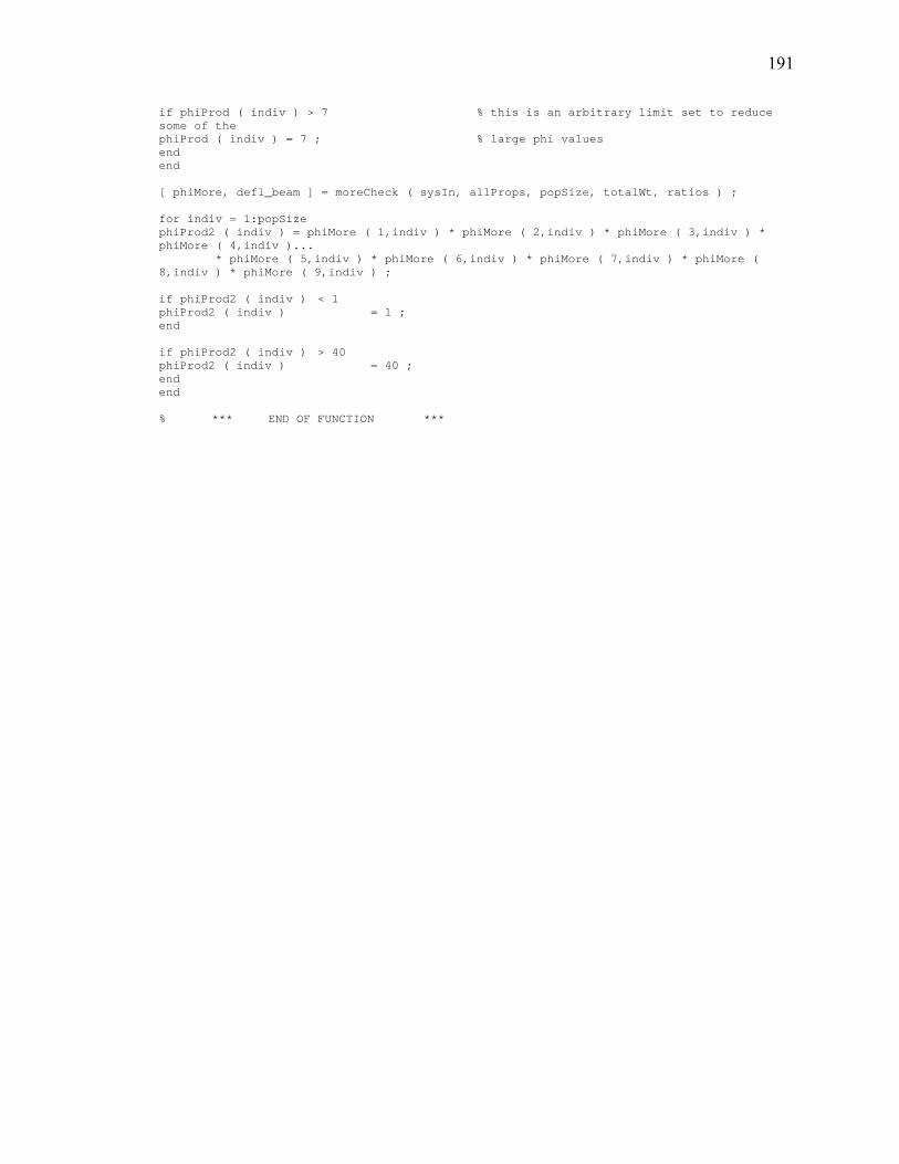
191
if phiProd ( indiv ) > 7 % this is an arbitrary limit set to reduce some of the phiProd ( indiv ) = 7 ; % large phi values end end [ phiMore, defl_beam ] = moreCheck ( sysIn, allProps, popSize, totalWt, ratios ) ; for indiv = 1:popSize phiProd2 ( indiv ) = phiMore ( 1,indiv ) * phiMore ( 2,indiv ) * phiMore ( 3,indiv ) * phiMore ( 4,indiv )... * phiMore ( 5,indiv ) * phiMore ( 6,indiv ) * phiMore ( 7,indiv ) * phiMore ( 8,indiv ) * phiMore ( 9,indiv ) ; if phiProd2 ( indiv ) < 1 phiProd2 ( indiv ) = 1 ; end if phiProd2 ( indiv ) > 40 phiProd2 ( indiv ) = 40 ; end end % *** END OF FUNCTION ***
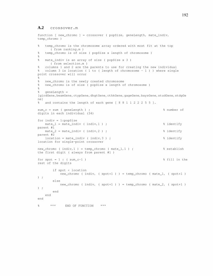
192
A.2 crossover.m function [ new_chromo ] = crossover ( popSize, geneLength, mate_indiv, temp_chromo ) % temp_chromo is the chromosome array ordered with most fit at the top ( from ranking.m ) % temp_chromo is of size ( popSize x length of chromosome ) % % mate_indiv is an array of size ( popSize x 3 ) ( from selection.m ) % columns 1 and 2 are the parents to use for creating the new individual % column 3 is location ( 1 to ( length of chromosome - 1 ) ) where single point crossover will occur % % new_chromo is the newly created chromosome % new_chromo is of size ( popSize x length of chromosome ) % % geneLength = [girdGene,beamGene,ctypGene,dhgtGene,cthkGene,gageGene,baysGene,studGene,stdgGene] % and contains the length of each gene [ 8 8 1 1 2 2 2 5 5 ]. sum_c = sum ( geneLength ) ; % number of digits in each individual (34) for indiv = 1:popSize mate_1 = mate_indiv ( indiv,1 ) ; % identify parent #1 mate_2 = mate_indiv ( indiv,2 ) ; % identify parent #2 location = mate_indiv ( indiv,3 ) ; % identify location for single-point crossover new_chromo ( indiv,1 ) = temp_chromo ( mate_1,1 ) ; % establish the first digit ( always from parent #1 ) for spot = 1 : ( sum_c-1 ) % fill in the rest of the digits if spot < location new_chromo ( indiv, ( spot+1 ) ) = temp_chromo ( mate_1, ( spot+1 ) ) ; else new_chromo ( indiv, ( spot+1 ) ) = temp_chromo ( mate_2, ( spot+1 ) ) ; end end end % *** END OF FUNCTION ***

193
A.3 decodeChromo.m function [ unknowns, allProps, totalWt, chromosome ] = decodeChromo ( sysIn, geneLength, chromosome ) % Purpose: % This subroutine decodes the binary string to integer values for later % use in assigning design variable values for fitness evaluation. % % Inputs: % % sysIn = [W,L,q,comp,desGen,Fy,fc,studDia,fu,studUp] % % geneLength = [girdGene,beamGene,ctypGene,dhgtGene,cthkGene,gageGene,baysGene,studGene,stdgGene] % and contains the length of each gene [ 8 8 1 1 2 2 2 5 5 ]. % % chromosome = 2-D array of chromosomes for current population % chromosome is of size ( popSize x length of chromosome ). % % Outputs: % % allProps = [ wfGird, wfBeam, stDeck, nBays, nStud, ngStud] % allProps is of size ( popSize x 68 ) where: % % unknowns = decoded chromosome values ( integer values ) % unknowns is of size ( popSize x number of genes ) % % totalWt(indiv) = wtBeams ( indiv ) + wtGirds ( indiv ) + wtDeck ( indiv ) % % chromosome has been modified by the gene repair function, and is now altered %---------------------------------------------------------------------------------------------------------------------- numUNKNO = length ( geneLength ) ; % Compute the number of design variables popSize = length ( chromosome ( :,1 ) ) ; % Compute the number of individuals in pop. chromLength = length ( chromosome ( 1,: ) ) ; % Compute the chromosome length %----- Decode the binary string chromosomes to an array of integers ( unknowns ) ------------------------------------- for i = 1:popSize % Loop over population bit = 1 ; % Set initial bit to the first one for j = 1:numUNKNO % Loop over unknowns unknowns ( i,j ) = 0 ; % Initialize unknown integer for allele = 1:geneLength ( j ) % Loop over alleles in gene if chromosome ( i,bit ) == 1 unknowns ( i,j ) = unknowns ( i,j ) + 2 ^ ( allele-1 ) ; % Compute binary contribution end if bit <= chromLength bit = bit + 1 ; % Increment the chromosome bit else

194
break % Break if chromosome length exceeded end end end end %---------------------------------------------------------------------------------------------------------------------- % Add "1" to the decoded design variable values to keep consistent % databases of information for design variables. % This makes the first choice #1 instead of #0. for i = 1:popSize for j = 1:numUNKNO unknowns ( i,j ) = unknowns ( i,j ) + 1 ; end end %---------------------------------------------------------------------------------------------------------------------- % Begin to convert chromosome data into real values for use in the problem *** % Start by creating an array, wfGird, which shows all of the wide flange properties *** % For the girder in each chromosome, 1 through 20. *** wfTab = xlsread ( 'AISC_W_Shapes.xls' ) ; wfGird = zeros ( popSize,15 ) ; for indiv = 1:popSize wfGird ( indiv,: ) = wfTab ( unknowns ( indiv,1 ) ,: ) ; end %---------------------------------------------------------------------------------------------------------------------- % Continue by creating an array, wfBeam, which shows all of the wide flange properties *** % For the beam in each chromosome, 1 through 20. *** wfBeam = zeros ( indiv,15 ) ; for indiv = 1:popSize wfBeam ( indiv,: ) = wfTab ( unknowns ( indiv,2 ), : ) ; end % -----------handle the concrete type, deck height, concrete thickness, and steel gage genes -------------------------- LW15Tab = xlsread ( 'LW_1_5.xls' ) ; LW30Tab = xlsread ( 'LW_3_0.xls' ) ; NW15Tab = xlsread ( 'NW_1_5.xls' ) ; NW30Tab = xlsread ( 'NW_3_0.xls' ) ; stDeck = zeros ( indiv,35 ) ; for indiv = 1:popSize if unknowns ( indiv,3 ) == 1 & unknowns ( indiv,4 ) == 1 ; stDeck ( indiv,: ) = NW15Tab ( unknowns ( indiv,6 ) + ( ( unknowns ( indiv,5 ) – 1 ) * 4 ),: ) ; elseif unknowns ( indiv,3 ) == 1 & unknowns ( indiv,4 ) == 2 ; stDeck ( indiv,: ) = NW30Tab ( unknowns ( indiv,6 ) + ( ( unknowns ( indiv,5 ) – 1 ) * 4),: ) ; elseif unknowns ( indiv,3 ) == 2 & unknowns ( indiv,4 ) == 1 ; stDeck ( indiv,: ) = LW15Tab ( unknowns ( indiv,6 ) + ( ( unknowns ( indiv,5 ) – 1 ) * 4 ),: ) ;
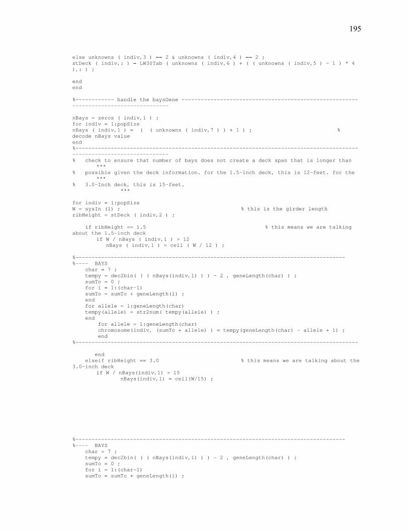
195
else unknowns ( indiv,3 ) == 2 & unknowns ( indiv,4 ) == 2 ; stDeck ( indiv,: ) = LW30Tab ( unknowns ( indiv,6 ) + ( ( unknowns ( indiv,5 ) – 1 ) * 4 ),: ) ; end end %------------ handle the baysGene ------------------------------------------------------------------------------------- nBays = zeros ( indiv,1 ) ; for indiv = 1:popSize nBays ( indiv,1 ) = ( ( unknowns ( indiv,7 ) ) + 1 ) ; % decode nBays value end %---------------------------------------------------------------------------------------------------------------------- % check to ensure that number of bays does not create a deck span that is longer than *** % possible given the deck information. for the 1.5-inch deck, this is 12-feet. for the *** % 3.0-Inch deck, this is 15-feet. *** for indiv = 1:popSize W = sysIn (1) ; % this is the girder length ribHeight = stDeck ( indiv,2 ) ; if ribHeight == 1.5 % this means we are talking about the 1.5-inch deck if W / nBays ( indiv,1 ) > 12 nBays ( indiv,1 ) = ceil ( W / 12 ) ; %------------------------------------------------------------------------------------ %---- BAYS char = 7 ; tempy = dec2bin( ( ( nBays(indiv,1) ) ) - 2 , geneLength(char) ) ; sumTo = 0 ; for i = 1:(char-1) sumTo = sumTo + geneLength(i) ; end for allele = 1:geneLength(char) tempy(allele) = str2num( tempy(allele) ) ; end for allele = 1:geneLength(char) chromosome(indiv, (sumTo + allele) ) = tempy(geneLength(char) - allele + 1) ; end %---------------------------------------------------------------------------------------- end elseif ribHeight == 3.0 % this means we are talking about the 3.0-inch deck if W / nBays(indiv,1) > 15 nBays(indiv,1) = ceil(W/15) ; %------------------------------------------------------------------------------------ %---- BAYS char = 7 ; tempy = dec2bin( ( ( nBays(indiv,1) ) ) - 2 , geneLength(char) ) ; sumTo = 0 ; for i = 1:(char-1) sumTo = sumTo + geneLength(i) ;

196
end for allele = 1:geneLength(char) tempy(allele) = str2num( tempy(allele) ) ; end for allele = 1:geneLength(char) chromosome(indiv, (sumTo + allele) ) = tempy(geneLength(char) - allele + 1) ; end %---------------------------------------------------------------------------------------- end end %---------------------------------------------------------------------------------------------------------------------- % *** Decode the integer designation for the number of studs *** % *** to the actual number of studs per half beam *** % *** number of studs per half beam (5 for 2^5 = 32 choices) *** % *** choices are from 0 to 124 per half beam in multiples of 4 *** nStud = zeros ( indiv,1 ) ; for indiv = 1:popSize nStud ( indiv,1 ) = ( ( unknowns ( indiv,8 ) ) – 1 ) * 4 ; end %----------- same for girder ------------------------------------------------------------------------------------------ ngStud = zeros ( indiv,1 ) ; for indiv = 1:popSize ngStud ( indiv,1 ) = ( ( unknowns ( indiv,9 ) ) – 1 ) * 4 ; end % Determine the maximum number of studs that will fit per half beam. BEAM % If the chromosome has too many, reduce the number of studs to the allowable amount. BEAM for indiv = 1:popSize girdLength = sysIn (1) ; % Length of girder in feet beamLength = sysIn (2) ; % Length of beam in feet studDia = sysIn (9) ; % Diameter of studs in inches (.75 TYP) deckSpace = stDeck ( indiv,5 ) ; % Spacing of valleys in inches (6-inch or 12-inch) flangeWidth = wfBeam ( indiv,6 ) ; % Width of the top flange for the beam trayWidth = stDeck ( indiv,9 ) ; % Measurement of the bottom of the valley in inches (1.75-inch or % 4.75-inch) if trayWidth == 1.75 % This means we are talking about the 1.5-inch deck rows = 1 ; % The number of rows per longitudinal direction is only 1 else % This means we are talking about the 3-inch deck rows = 2 ; % The number of rows per longitudinal direction is 2 end % Assuming .75 DIA studs, center-to-center spacing of 4 * DIA = 3 % + 1 DIA = 3.75-inches which will fit within % a 4.75-inch valley % It turns out that either way, there are 2 rows per 12-inches partners = floor ( ( flangeWidth - studDia ) / ( 4 * studDia ) ) + 1 ; % partners is how many stud will fit side by side
197
% in a valley according to spacing of 4 * DIA perHalfBeam ( indiv ) = floor ( beamLength / 2 ) * 2 * partners ; % perHalfBeam is the maximum number of studs that will fit per % half beam end %---------------------------------------------------------------------------------------------------------------------- %---- BEAM LOCATION 1 -------------------------------------------------------------------------------------- char = 8 ; tempy = dec2bin ( ( floor ( nStud ( indiv,1 ) / 4 ) ) , geneLength ( char ) ) ; sumTo = 0 ; for i = 1:( char-1 ) sumTo = sumTo + geneLength (i) ; end for allele = 1:geneLength ( char ) tempy ( allele ) = str2num ( tempy ( allele ) ) ; end for allele = 1:geneLength ( char ) chromosome ( indiv, ( sumTo + allele ) ) = tempy ( geneLength ( char ) - allele + 1 ) ; end %---------------------------------------------------------------------------------------------------------------------- end end end %---------------------------------------------------------------------------------------------------------------------- % Determine the maximum number of studs that will fit per half girder. GIRDER % If the chromosome has too many, reduce the number of studs to the allowable amount. GIRDER for indiv = 1:popSize girdLength = sysIn (1) ; % girder length in feet beamLength = sysIn (2) ; % beam length in feet studDia = sysIn (9) ; % stud diameter in inches (.75 TYP) trayWidth = stDeck ( indiv,9 ) ; % Measurement of the bottom of the valley in inches (1.75-in or 4.75-in) flangeWidth = wfGird ( indiv,6 ) ; % Width of the top flange for the girder if trayWidth == 1.75 % This means we are talking about the 1.5-inch deck if flangeWidth >= 12.00 % For the 1.5-inch deck: if the girder flange width % is greater than 12.0-inches rows = 2 ; % Then two deck valleys will lay on top of the girder else % otherwise rows = 1 ; % only one deck valley will lay on top of the girder end else % This means we are talking about the 3-inch deck if studDia < 1.0 % For stud diameters less than 1-inch rows = 2 ; % only one deck valley will ay on top of the girder for two rows total else % For stud diameters greater than or equal to 1-inch
198
rows = 1 ; % only one deck valley will lay on top of the girder with only one row end end perHalfGird ( indiv ) = rows * floor ( girdLength / studDia ) ; % This just worked out this way % its actually ( girdLength / 2 ) * 12 / ( 6 * DIA ) end % ---- GIRDER LOCATION 1 --------------------------------------------------------------------------------------------- char = 9 ; tempy = dec2bin ( ( floor ( ngStud ( indiv,1 ) / 4 ) ) , geneLength ( char ) ) ; sumTo = 0 ; for i = 1:( char-1 ) sumTo = sumTo + geneLength (i) ; end for allele = 1:geneLength ( char ) tempy ( allele ) = str2num ( tempy ( allele ) ) ; end for allele = 1:geneLength ( char ) chromosome ( indiv, ( sumTo + allele ) ) = tempy ( geneLength ( char ) - allele + 1 ) ; end %---------------------------------------------------------------------------------------------------------------------- end end end %---- Determine the minimum number of studs per half beam because of maximum spacing requirements -------------------- %---- If there are too few, adjust up to the minimum amount. ---------------------------------------------------- %---- BEAM BEAM BEAM BEAM BEAM BEAM BEAM BEAM BEAM BEAM BEAM BEAM BEAM BEAM ----------------------------------------- for indiv = 1:popSize cThick ( indiv ) = stDeck ( indiv,3 ) ; beamLength = sysIn (2) ; maxBSpace ( indiv ) = floor ( 8 * cThick ( indiv ) ) ; minBStud ( indiv ) = ceil ( ( 12 * beamLength / 2 ) / maxBSpace ( indiv ) ) ; end % --------------------------------------------------------------------------------------------------------------------- % ---- BEAM LOCATION 2 ----------------------------------------------------------------------------------------------- char = 8 ; tempy = dec2bin ( ( floor ( nStud ( indiv,1 ) / 4 ) ) , geneLength ( char ) ) ; sumTo = 0 ; for i = 1:( char-1 ) sumTo = sumTo + geneLength (i) ; end for allele = 1:geneLength ( char ) tempy ( allele ) = str2num ( tempy ( allele ) ) ; end for allele = 1:geneLength ( char ) chromosome ( indiv, ( sumTo + allele ) ) = tempy ( geneLength ( char ) - allele + 1 ) ; end
199
% --------------------------------------------------------------------------------------------------------------------- end end end % Determine the minimum number of studs per half girder because GIRDER --------------------------------------- % of maximum spacing requirements. ---------------------------------------------------- % If there are too few, adjust up to the minimum amount. ---------------------------------------------------- for indiv = 1:popSize cThick ( indiv ) = stDeck ( indiv,3 ) ; girdLength = sysIn (1) ; maxGSpace ( indiv ) = floor ( 8 * cThick ( indiv ) ) ; minGStud ( indiv ) = ceil ( ( 12 * girdLength / 2 ) / maxGSpace ( indiv ) ) ; end % --------------------------------------------------------------------------------------------------------------------- % ---- GIRDER LOCATION 2 --------------------------------------------------------------------------------------------- char = 9 ; tempy = dec2bin ( ( floor ( ngStud ( indiv,1 ) / 4 ) ) , geneLength ( char ) ) ; sumTo = 0 ; for i = 1:( char-1 ) sumTo = sumTo + geneLength (i) ; end for allele = 1:geneLength ( char ) tempy ( allele ) = str2num ( tempy ( allele ) ) ; end for allele = 1:geneLength ( char ) chromosome ( indiv, ( sumTo + allele ) ) = tempy ( geneLength ( char ) - allele + 1 ) ; end % --------------------------------------------------------------------------------------------------------------------- end end end allProps = [wfGird,wfBeam,stDeck,nBays,nStud,ngStud] ; % Find the total dead weight of the flooring components, including concrete: W = sysIn (1) ; L = sysIn (2) ; wtBeams = zeros ( indiv,1 ) ; wtGirds = zeros ( indiv,1 ) ; wtDeck = zeros ( indiv,1 ) ; totalWt = zeros ( indiv,1 ) ; for indiv = 1:popSize wtBeams ( indiv ) = ( ( nBays ( indiv,1 ) + 1 ) * wfBeam ( indiv,2 ) ) / W ; % answer in psf wtGirds ( indiv ) = ( 2 * wfGird ( indiv,2 ) ) / L ; % answer in psf wtDeck ( indiv ) = stDeck ( indiv,6 ) + stDeck ( indiv,8 ) ; % answer in psf totalWt ( indiv ) = wtBeams ( indiv ) + wtGirds ( indiv ) + wtDeck ( indiv ) ; % totalWt is used % only for self- % weight of the % system

200
end % *** END OF FUNCTION ***
201
A.4 eliminate.m function [ num_small_vibe, pop_vibe ] = eliminate ( gather_counter, chromLength, vibe_chromo ) ; % vibe_chromo is the array containing all the chromosome material (used to be "chromosome") % chromLength is just the length (number of digits) % gather_counter is the number of individuals in the array, vibe_chromo (they were previously "gathered") % num_small_vibe is the new array, containing only unique individuals % pop_vibe is the number of individuals in the new array str_vibe_chromo = num2str ( vibe_chromo ) ; % this is vibe_chromo in a string array % using MATLAB's number to string converter % put first individual in the new array, small_vibe ( this is a string array ) small_vibe ( 1,: ) = str_vibe_chromo ( 1,: ) ; % put first individual in the new array pop_vibe = 1 ; % the population of the new array is one for individuals = 2:gather_counter % this is all of the remaining individuals in the % original array, str_vibe_chromo I = strmatch ( str_vibe_chromo ( individuals,: ) , small_vibe, 'exact' ) ; % see "help strmatch" this line % compares each % individual in the original % array with the contents % of the new array, and returns % matches in []. B = isempty (I) ; % see "help isempty(I)" this function returns % 1 if the solution set [] is empty if B == 1 % this means there are no matches % in the new array pop_vibe = pop_vibe + 1 ; % increment the counter small_vibe ( pop_vibe,: ) = str_vibe_chromo ( individuals,: ) ; % add current individual to the new array end end num_small_vibe = str2num ( small_vibe ) ; % convert back to number array % *** END OF FUNCTION ***
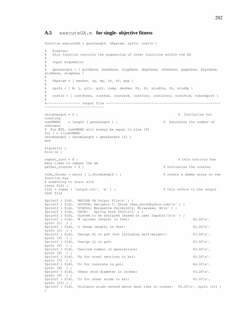
202
A.5 executeGA.m for single- objective fitness function executeGA ( geneLength, GAparam, sysIn, costIn ) % Purpose: % This function controls the sequencing of other functions within the GA % % Input Arguments: % % geneLength = [ girdGene, beamGene, ctypGene, dhgtGene, cthkGene, gageGene, baysGene, studGene, stdgGene ] % % GAparam = [ maxGen, cp, mp, fs, ef, pop ] % % sysIn = [ W, L, q(1), q(2), comp, desGen, Fy, fc, studDia, fu, studUp ] % % costIn = [ costSteel, costFab, costDeck, costConc, costLConc, costStud, vibeImport ] % %----------------- output file ---------------------------------------------------------------------------------------- chromLength = 0 ; % Initialize for counting numUNKNO = length ( geneLength ) ; % Determine the number of unknowns % For BTS, numUNKNO will always be equal to nine (9) for i = 1:numUNKNO chromLength = chromLength + geneLength (i) ; end figure(1) ; hold on ; repeat_runs = 8 ; % this controls how many times to repeat the GA gather_counter = 0 ; % initialize the counter vibe_chromo = zeros ( 1,chromLength ) ; % create a dummy array so the function has % something to start with clear fid1 ; fid1 = fopen ( 'output.txt', 'w' ) ; % this refers to the output text file fprintf ( fid1, 'MATLAB GA Output File\n' ) ; fprintf ( fid1, 'AUTHOR: Benjamin T. Shock ([email protected])\n' ) ; fprintf ( fid1, 'SCHOOL: Marquette University, Milwaukee, WI\n' ) ; fprintf ( fid1, 'DATE: Spring Term 2003\n\n' ) ; fprintf ( fid1, 'System to be analyzed (based on user inputs):\n\n' ) ; fprintf ( fid1, 'W (girder length) in feet: %2.0f\n', sysIn (1) ) ; fprintf ( fid1, 'L (beam length) in feet: %2.0f\n', sysIn (2) ) ; fprintf ( fid1, 'Design DL in psf (not including self-weight): %3.0f\n', sysIn (3) ) ; fprintf ( fid1, 'Design LL in psf: %3.0f\n', sysIn (4) ) ; fprintf ( fid1, 'Desired number of generations: %3.0f\n', sysIn (6) ) ; fprintf ( fid1, 'Fy for steel sections in ksi: %2.0f\n', sysIn (7) ) ; fprintf ( fid1, 'Fc for concrete in psi: %4.0f\n', sysIn (8) ) ; fprintf ( fid1, 'Shear stud diameter in inches: %3.2f\n', sysIn (9) ) ; fprintf ( fid1, 'fu for shear studs in ksi: %2.0f\n', sysIn (10) ) ; fprintf ( fid1, 'Distance studs extend above deck ribs in inches: %3.2f\n', sysIn (11) ) ;

203
fprintf ( fid1, 'Cost per pound of steel in dollars: %3.2f\n', costIn (1) ) ; fprintf ( fid1, 'Cost per pound for fabrication in dollars: %3.2f\n', costIn (2) ) ; fprintf ( fid1, 'Cost per pound of deck in dollars: %3.2f\n', costIn (3) ) ; fprintf ( fid1, 'Cost per cubic yard of NW concrete in dollars: %3.0f\n', costIn (4) ) ; fprintf ( fid1, 'Cost per cubic yard of LW concrete in dollars: %3.0f\n', costIn (5) ) ; fprintf ( fid1, 'Cost per shear stud in dollars: %3.0f\n', costIn (6) ) ; fprintf ( fid1, 'Cut point for 75-per./25-per. scheme (0 to 100): %3.0f\n', GAparam (2) ) ; fprintf ( fid1, 'Mutation probability (0 to 1): %3.3f\n', GAparam (3) ) ; fprintf ( fid1, 'Elitism ( 0 is OFF, 1 is ON ): %1.0f\n', GAparam (5) ) ; fprintf ( fid1, 'With elitism on, percentage of parents allowed to \n' ) ; fprintf ( fid1, 'proceed to next generation. 100-percent means that \n' ) ; fprintf ( fid1, 'the most fit 50-percent of the parents will form \n' ) ; fprintf ( fid1, '50-percent of the next generation. %3.0f\n', GAparam (4) ) ; fprintf ( fid1, 'Population size: %3.0f\n', GAparam (6) ) ; fprintf ( fid1, 'Number of runs: %3.0f\n', repeat_runs ) ; fprintf(fid1, '\nPLOT COLORS: 1-black 2-black(--) 3-blue 4-blue(--)\n' ) ; fprintf ( fid1, '5-green 6-green(--) 7-red 8-red(--) 9-yellow 10-yellow(--)\n' ) ; %----------------- end of output file --------------------------------------------------------------------------------- for repeat = 1:repeat_runs % start the repeating loop % *** Build the Initial Population of Random Strings *** Generation = 1 ; % Initialize the generation counter popSize = GAparam (6) ; % Population size % *** Create the initial population of chromosomes *** [ chromosome ] = InitialPopulation ( popSize, geneLength ) ; % *** Decode chromosomes to unknown real values *** [ unknowns, allProps, totalWt, chromosome ] = decodeChromo ( sysIn, geneLength, chromosome ) ; % ********************************************************************************************************* % when using ap_g as the thirteenth penalty, floorVib.m must be used in this location: * % * % *** Pass individuals through floor vibe function *** * % * % [ f_n, Weqv, ap_g ] = floorVib ( allProps, sysIn, chromosome, GAparam ) ; * % *
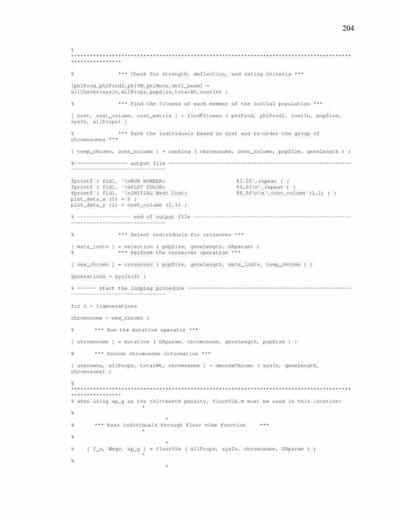
204
% ********************************************************************************************************* % *** Check for strength, deflection, and rating criteria *** [phiProd,phiProd2,phiVM,phiMore,defl_beam] = allChecks(sysIn,allProps,popSize,totalWt,costIn) ; % *** Find the fitness of each member of the initial population *** [ cost, cost_column, cost_matrix ] = findFitness ( phiProd, phiProd2, costIn, popSize, sysIn, allProps) ; % *** Rank the individuals based on cost and re-order the group of chromosomes *** [ temp_chromo, cost_column ] = ranking ( chromosome, cost_column, popSize, geneLength ) ; %----------------- output file ---------------------------------------------------------------------------------------- fprintf ( fid1, '\nRUN NUMBER: %3.0f',repeat ) ; fprintf ( fid1, '\nPLOT COLOR: %3.0f\n',repeat ) ; fprintf ( fid1, '\nINITIAL Best Cost: %8.0f\n\n',cost_column (1,1) ) ; plot_data_x (1) = 0 ; plot_data_y (1) = cost_column (1,1) ; % ----------------- end of output file -------------------------------------------------------------------------------- % *** Select individuals for crossover *** [ mate_indiv ] = selection ( popSize, geneLength, GAparam) ; % *** Perform the crossover operation *** [ new_chromo ] = crossover ( popSize, geneLength, mate_indiv, temp_chromo ) ; generations = sysIn(6) ; % ------ start the looping procedure ---------------------------------------------------------------------------------- for i = 1:generations chromosome = new_chromo ; % *** Run the mutation operator *** [ chromosome ] = mutation ( GAparam, chromosome, geneLength, popSize ) ; % *** Decode chromosome information *** [ unknowns, allProps, totalWt, chromosome ] = decodeChromo ( sysIn, geneLength, chromosome) ; % ********************************************************************************************************* % when using ap_g as the thirteenth penalty, floorVib.m must be used in this location: * % * % *** Pass individuals through floor vibe function *** * % * % [ f_n, Weqv, ap_g ] = floorVib ( allProps, sysIn, chromosome, GAparam ) ; * % *

205
% ********************************************************************************************************* % *** Perform checks on deflection, strength, rating *** [ phiProd, phiProd2, phiVM, phiMore, defl_beam ] = allChecks ( sysIn, allProps, popSize, totalWt, costIn ) ; % *** Evaluate the fitness of each member in the population *** [ cost, cost_column, cost_matrix ] = findFitness ( phiProd, phiProd2, costIn, popSize, sysIn, allProps ) ; % *** Evaluate frequency, equivalent weight, and acceleration for each individual in the population *** [ f_n, Weqv, ap_g] = floorVib ( allProps, sysIn, chromosome, GAparam ) ; % *** Perform the ranking operation on the population *** [ temp_chromo, cost_column ] = ranking ( chromosome, cost_column, popSize, geneLength ) ; % ----------------- output file --------------------------------------------------------------------------------------- fprintf ( fid1, 'GENERATION %3.0f Best Cost: %8.0f\n',i,cost_column (1,1) ) ; plot_data_x (1+i) = i ; plot_data_y (1+i) = cost_column ( 1,1 ) ; % ---------------------- end of output file --------------------------------------------------------------------------- % *** Select individuals for crossover *** [ mate_indiv ] = selection ( popSize, geneLength, GAparam ) ; % *** Perform the crossover operation *** [ new_chromo ] = crossover ( popSize, geneLength, mate_indiv, temp_chromo ) ; end % end of generation looping % *** Gather feasible individuals *** [ gather_counter, vibe_chromo ] = gather ( repeat, chromLength, phiProd, phiProd2, popSize, gather_counter, … temp_chromo, vibe_chromo ) ; % ---------------------- output file ---------------------------------------------------------------------------------- fprintf ( fid1, '\nCosts for the ten "fittest" individuals in the final generation' ) ; fprintf ( fid1, '\nindiv beam gird deck LWconc NWconc bmStud gdStud sum cost\n\n' ) ; for result = 1:10 location = cost_column ( result,2 ) ; beamCost ( result ) = cost_matrix ( location,1 ) ; girdCost ( result ) = cost_matrix ( location,2 ) ; deckCost ( result ) = cost_matrix ( location,3 ) ; LWcost ( result ) = cost_matrix ( location,4 ) ; NWcost ( result ) = cost_matrix ( location,5 ) ; beamStudCost ( result ) = cost_matrix ( location,6 ) ; girdStudCost ( result ) = cost_matrix ( location,7 ) ; sum_e ( result ) = cost_matrix ( location,8 ) ; cost ( result ) = cost_matrix ( location,9 ) ;
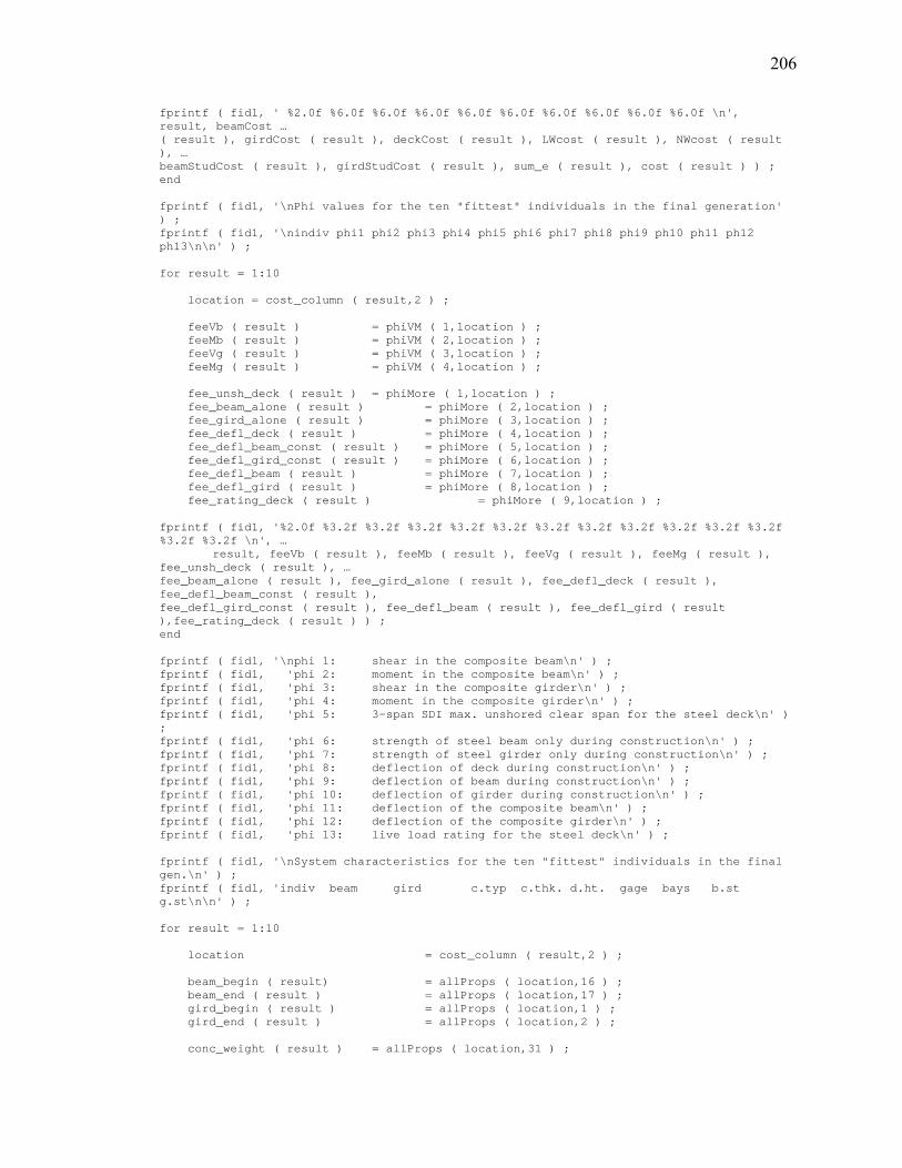
206
fprintf ( fid1, ' %2.0f %6.0f %6.0f %6.0f %6.0f %6.0f %6.0f %6.0f %6.0f %6.0f \n', result, beamCost … ( result ), girdCost ( result ), deckCost ( result ), LWcost ( result ), NWcost ( result ), … beamStudCost ( result ), girdStudCost ( result ), sum_e ( result ), cost ( result ) ) ; end fprintf ( fid1, '\nPhi values for the ten "fittest" individuals in the final generation' ) ; fprintf ( fid1, '\nindiv phi1 phi2 phi3 phi4 phi5 phi6 phi7 phi8 phi9 ph10 ph11 ph12 ph13\n\n' ) ; for result = 1:10 location = cost_column ( result,2 ) ; feeVb ( result ) = phiVM ( 1,location ) ; feeMb ( result ) = phiVM ( 2,location ) ; feeVg ( result ) = phiVM ( 3,location ) ; feeMg ( result ) = phiVM ( 4,location ) ; fee_unsh_deck ( result ) = phiMore ( 1,location ) ; fee_beam_alone ( result ) = phiMore ( 2,location ) ; fee_gird_alone ( result ) = phiMore ( 3,location ) ; fee_defl_deck ( result ) = phiMore ( 4,location ) ; fee_defl_beam_const ( result ) = phiMore ( 5,location ) ; fee_defl_gird_const ( result ) = phiMore ( 6,location ) ; fee_defl_beam ( result ) = phiMore ( 7,location ) ; fee_defl_gird ( result ) = phiMore ( 8,location ) ; fee_rating_deck ( result ) = phiMore ( 9,location ) ; fprintf ( fid1, '%2.0f %3.2f %3.2f %3.2f %3.2f %3.2f %3.2f %3.2f %3.2f %3.2f %3.2f %3.2f %3.2f %3.2f \n', … result, feeVb ( result ), feeMb ( result ), feeVg ( result ), feeMg ( result ), fee_unsh_deck ( result ), … fee_beam_alone ( result ), fee_gird_alone ( result ), fee_defl_deck ( result ), fee_defl_beam_const ( result ), fee_defl_gird_const ( result ), fee_defl_beam ( result ), fee_defl_gird ( result ),fee_rating_deck ( result ) ) ; end fprintf ( fid1, '\nphi 1: shear in the composite beam\n' ) ; fprintf ( fid1, 'phi 2: moment in the composite beam\n' ) ; fprintf ( fid1, 'phi 3: shear in the composite girder\n' ) ; fprintf ( fid1, 'phi 4: moment in the composite girder\n' ) ; fprintf ( fid1, 'phi 5: 3-span SDI max. unshored clear span for the steel deck\n' ) ; fprintf ( fid1, 'phi 6: strength of steel beam only during construction\n' ) ; fprintf ( fid1, 'phi 7: strength of steel girder only during construction\n' ) ; fprintf ( fid1, 'phi 8: deflection of deck during construction\n' ) ; fprintf ( fid1, 'phi 9: deflection of beam during construction\n' ) ; fprintf ( fid1, 'phi 10: deflection of girder during construction\n' ) ; fprintf ( fid1, 'phi 11: deflection of the composite beam\n' ) ; fprintf ( fid1, 'phi 12: deflection of the composite girder\n' ) ; fprintf ( fid1, 'phi 13: live load rating for the steel deck\n' ) ; fprintf ( fid1, '\nSystem characteristics for the ten "fittest" individuals in the final gen.\n' ) ; fprintf ( fid1, 'indiv beam gird c.typ c.thk. d.ht. gage bays b.st g.st\n\n' ) ; for result = 1:10 location = cost_column ( result,2 ) ; beam_begin ( result) = allProps ( location,16 ) ; beam_end ( result ) = allProps ( location,17 ) ; gird_begin ( result ) = allProps ( location,1 ) ; gird_end ( result ) = allProps ( location,2 ) ; conc_weight ( result ) = allProps ( location,31 ) ;

207
conc_thick (result ) = allProps ( location,33 ) ; deck_height ( result ) = allProps ( location,32 ) ; deck_gage ( result ) = allProps ( location,34 ) ; bays ( result ) = allProps ( location,66 ) ; beam_studs ( result ) = allProps ( location,67 ) ; gird_studs ( result ) = allProps ( location,68 ) ; fprintf ( fid1, '%2.0f w%2.0fx%3.0f w%2.0fx%3.0f %3.0f %2.1f %2.1f %2.0f %1.0f %3.0f %3.0f\n', result, … beam_begin ( result ), beam_end ( result ), gird_begin ( result ), gird_end ( result ), conc_weight ( result ), … conc_thick ( result ), deck_height ( result ), deck_gage ( result ), bays ( result ), beam_studs ( result ), … gird_studs ( result ) ) ; end fprintf ( fid1, '\nBeam deflections for the ten "fittest" individuals in the final gen.\n' ) ; fprintf ( fid1, 'indiv deflection\n\n' ) ; for result = 1:10 location = cost_column ( result,2 ) ; beam_deflection ( result ) = defl_beam ( location ) ; fprintf ( fid1, '%2.0f %5.4f\n', result, beam_deflection ( result ) ) ; end fprintf ( fid1, '\nNatural frequencies for the ten "fittest" individuals in the final gen.\n' ) ; fprintf ( fid1, 'indiv natural frequency\n\n' ) ; for result = 1:10 location = cost_column ( result,2 ) ; nat_freq ( result ) = f_n ( location ) ; fprintf ( fid1, '%2.0f %3.2f\n', result, nat_freq ( result ) ) ; end fprintf ( fid1, '\nDimensionless acceleration values for the ten "fittest" individuals in the final gen.\n' ) ; fprintf ( fid1, 'indiv ap / g \n\n' ) ; for result = 1:10 location = cost_column ( result,2 ) ; accel ( result ) = ap_g ( location ) ; fprintf ( fid1, '%2.0f %5.4f\n', result, accel ( result ) ) ; end % ----------------- output file --------------------------------------------------------------------------------------- % --------------------------------------------------------------------------------------------------------------------- if repeat == 1 plot ( plot_data_x, plot_data_y, 'k' ) ; xlabel ( 'Generation' ) ; ylabel ( 'Cost for "fittest" individual' ) ; title ( 'Convergence Trajectory Plot, MATLAB GA' ) ; elseif repeat == 2 plot ( plot_data_x, plot_data_y,'k--' ) ; elseif repeat == 3 plot ( plot_data_x, plot_data_y, 'b' ) ;
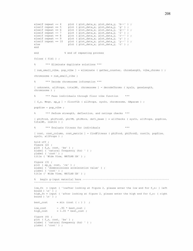
208
elseif repeat == 4 plot ( plot_data_x, plot_data_y, 'b--' ) ; elseif repeat == 5 plot ( plot_data_x, plot_data_y, 'g' ) ; elseif repeat == 6 plot ( plot_data_x, plot_data_y, 'g--' ) ; elseif repeat == 7 plot ( plot_data_x, plot_data_y, 'r' ) ; elseif repeat == 8 plot ( plot_data_x, plot_data_y, 'r--' ) ; elseif repeat == 9 plot ( plot_data_x, plot_data_y, 'y' ) ; elseif repeat == 10 plot ( plot_data_x, plot_data_y, 'y--' ) ; else plot ( plot_data_x, plot_data_y, 'c' ) ; end end % end of repeating process fclose ( fid1 ) ; % *** Eliminate duplicate solutions *** [ num_small_vibe, pop_vibe ] = eliminate ( gather_counter, chromLength, vibe_chromo ) ; chromosome = num_small_vibe ; % *** Decode chromosome information *** [ unknowns, allProps, totalWt, chromosome ] = decodeChromo ( sysIn, geneLength, chromosome ) ; % *** Pass individuals through floor vibe function *** [ f_n, Weqv, ap_g ] = floorVib ( allProps, sysIn, chromosome, GAparam ) ; popSize = pop_vibe ; % *** Peform strength, deflection, and ratings checks *** [ phiProd, phiProd2, phiVM, phiMore, defl_beam ] = allChecks ( sysIn, allProps, popSize, totalWt, costIn ) ; % *** Evaluate fitness for individuals *** [ cost, cost_column, cost_matrix ] = findFitness ( phiProd, phiProd2, costIn, popSize, sysIn, allProps ) ; hold off ; figure (2) ; plot ( f_n, cost, 'bx' ) ; xlabel ( 'natural frequency (hz) ' ) ; ylabel ( 'cost' ) ; title ( 'Wide View, MATLAB GA' ) ; figure (3) ; plot ( ap_g, cost, 'rx' ) ; xlabel ( 'dimensionless acceleration value' ) ; ylabel ( 'cost' ) ; title (' Wide View, MATLAB GA' ) ; % begin g-input material here --------------------------------------------------------------------------------------- low_fn = input ( '\nafter looking at figure 2, please enter the low end for f_n: ( left bound ) \n' ) ; high_fn = input ( 'after looking at figure 2, please enter the high end for f_n: ( right bound ) \n' ) ; best_cost = min (cost ( : ) ) ; low_cost = .95 * best_cost ; high_cost = 1.35 * best_cost ; figure (4) ; plot ( f_n, cost, 'bx' ) ; xlabel ( 'natural frequency (hz) ' ) ; ylabel ( 'cost' ) ;
209
title ( 'Zoomed View, MATLAB GA' ) ; axis ( [ low_fn high_fn low_cost high_cost ] ) low_apg = input ( '\nafter looking at figure 3, please enter the low end for ap/g: ( left bound ) \n' ) ; high_apg = input ( 'after looking at figure 3, please enter the high end for ap/g: ( right bound ) \n' ) ; best_cost = min ( cost ( : ) ) ; low_cost = .95 * best_cost ; high_cost = 1.35 * best_cost ; figure (5) ; plot ( ap_g, cost, 'rx' ) ; xlabel ( 'dimensionless acceleration' ) ; ylabel ( 'cost' ) ; title ( 'Zoomed View, MATLAB GA' ) ; axis ( [ low_apg high_apg low_cost high_cost ] ) % continue g-input -------------------------------------------------------------------------------------------------- msg1 = sprintf ( 'Place the cursor over the point you would like to ' ) ; msg1 = [ msg1,sprintf ( 'investigate and then press the LEFT mouse button. ' ) ] ; msg1 = [ msg1,sprintf ( 'Repeat for desired number of points, then hit ENTER.' ) ] ; h = msgbox ( msg1 ) ; [ acceleration, cost_graph ] = ginput ; length_a = length ( acceleration ) ; for indiv = 1:length_a rounded_accel_plot ( indiv ) = ( round ( acceleration ( indiv ) * 100 ) ) / 100 ; rounded_cost_plot ( indiv ) = ( round ( cost_graph ( indiv ) / 1000 ) ) * 1000 ; end for indiv = 1:popSize rounded_ap_g ( indiv ) = ( round ( ap_g ( indiv ) * 100 ) ) / 100 ; rounded_cost ( indiv ) = ( round (cost ( indiv ) / 1000 ) ) * 1000 ; end clear fid2 ; fid2 = fopen ( 'results.txt', 'w' ) ; fprintf ( fid2, '\nSystem characteristics for the individuals chosen in figure 5\n' ) ; fprintf ( fid2, 'indiv beam gird c.tp c.thk. d.ht. gag bay b.st g.st $ ap/g\n\n' ) ; for mouse_clicks = 1:length_a for popul = 1:popSize if rounded_ap_g ( popul ) == rounded_accel_plot ( mouse_clicks ) ... & rounded_cost ( popul ) == rounded_cost_plot ( mouse_clicks ) ; fprintf ( fid2, '\n' ) ; % if they match up, then report the system characteristics for indiv: popul fprintf ( fid2, '%3.0f w%2.0fx%3.0f w%2.0fx%3.0f %3.0f %2.1f %2.1f %2.0f %1.0f %3.0f %3.0f %6.0f %2.2f\n', … popul, allProps ( popul,16 ), allProps ( popul,17 ), allProps ( popul,1 ), allProps ( popul,2 ), … allProps ( popul,31 ), allProps ( popul,33 ), allProps ( popul,32 ), allProps ( popul,34 ), … allProps ( popul,66 ), allProps ( popul,67 ), allProps ( popul,68 ), cost ( popul ), ap_g ( popul ) ) ; end end end fclose ( fid2 ) ; % *** END OF PROGRAM ***
210
A.6 executeGA.m for multi- objective fitness function executeGA ( geneLength, GAparam, sysIn, costIn ) % Purpose: % This function controls the sequencing of other functions within the GA % % Input Arguments: % % geneLength = [ girdGene, beamGene, ctypGene, dhgtGene, cthkGene, gageGene, baysGene, studGene, stdgGene ] % % GAparam = [ maxGen, cp, mp, fs, ef, pop ] % % sysIn = [ W, L, q(1), q(2), comp, desGen, Fy, fc, studDia, fu, studUp ] % % costIn = [ costSteel, costFab, costDeck, costConc, costLConc, costStud, vibeImport ] %----------------- output file ---------------------------------------------------------------------------------------- chromLength = 0 ; % Initialize for counting numUNKNO = length(geneLength) ; % Determine the number of unknowns % For BTS, numUNKNO will always be equal to eight (9) for i = 1:numUNKNO chromLength = chromLength + geneLength(i) ; end clear fid1 ; fid1 = fopen('output.txt', 'w') ; fprintf ( fid1, 'MATLAB GA Output File\n' ) ; fprintf ( fid1, 'AUTHOR: Benjamin T. Shock ( [email protected] )\n' ) ; fprintf ( fid1, 'SCHOOL: Marquette University, Milwaukee, WI\n' ) ; fprintf ( fid1, 'DATE: Spring Term 2003\n\n' ) ; fprintf ( fid1, 'System to be analyzed ( based on user inputs ): \n\n' ) ; fprintf ( fid1, 'W ( girder length ) in feet: %2.0f\n', sysIn ( 1 ) ) ; fprintf ( fid1, 'L ( beam length ) in feet: %2.0f\n', sysIn ( 2 ) ) ; fprintf ( fid1, 'Design DL in psf (not including self-weight): %3.0f\n', sysIn ( 3 ) ) ; fprintf ( fid1, 'Design LL in psf: %3.0f\n', sysIn ( 4 ) ) ; fprintf ( fid1, 'Desired number of generations: %3.0f\n', sysIn ( 6 ) ) ; fprintf ( fid1, 'Fy for steel sections in ksi: %2.0f\n', sysIn ( 7 ) ) ; fprintf ( fid1, 'Fc for concrete in psi: %4.0f\n', sysIn ( 8 ) ) ; fprintf ( fid1, 'Shear stud diameter in inches: %3.2f\n', sysIn ( 9 ) ) ; fprintf ( fid1, 'fu for shear studs in ksi: %2.0f\n', sysIn (10 ) ) ; fprintf ( fid1, 'Distance studs extend above deck ribs in inches: %3.2f\n', sysIn (11 ) ) ; fprintf ( fid1, 'Cost per pound of steel in dollars: %3.2f\n', costIn (1) ) ; fprintf ( fid1, 'Cost per pound for fabrication in dollars: %3.2f\n', costIn (2) ) ; fprintf ( fid1, 'Cost per pound of deck in dollars: %3.2f\n', costIn (3) ) ; fprintf ( fid1, 'Cost per cubic yard of NW concrete in dollars: %3.0f\n', costIn (4) ) ; fprintf ( fid1, 'Cost per cubic yard of LW concrete in dollars: %3.0f\n', costIn (5) ) ; fprintf ( fid1, 'Cost per shear stud in dollars: %3.0f\n', costIn (6) ) ;
211
fprintf ( fid1, 'Cut point for 75-per./25-per. scheme (0 to 100): %3.0f\n', GAparam (2) ) ; fprintf ( fid1, 'Mutation probability (0 to 1): %3.3f\n', GAparam (3) ) ; fprintf ( fid1, 'Elitism ( 0 is OFF, 1 is ON ): %1.0f\n', GAparam (5) ) ; fprintf ( fid1, 'With elitism on, percentage of parents allowed to \n' ) ; fprintf ( fid1, 'proceed to next generation. 100-percent means that \n' ) ; fprintf ( fid1, 'the most fit 50-percent of the parents will form \n' ) ; fprintf ( fid1, '50-percent of the next generation. %3.0f\n', GAparam (4) ) ; fprintf ( fid1, 'Population size: %3.0f\n', GAparam (6) ) ; % *** Build the Initial Population of Random Strings *** Generation = 1 ; % Initialize the generation counter popSize = GAparam(6) ; % Population size % *** Create the initial population of chromosomes *** [ chromosome ] = InitialPopulation ( popSize , geneLength ) ; % *** Decode chromosomes to unknown real values *** [ unknowns,allProps,totalWt,totalWt_beam,chromosome ] = decodeChromo ( sysIn,geneLength,chromosome ) ; [ phiProd,phiProd2,phiVM,phiMore,defl_beam,defl_gird ] = allChecks ( sysIn,allProps,popSize,totalWt,costIn ) ; % *** Find the fitness of each member of the initial population *** [ cost,cost_column,cost_matrix,ap_g ] = findFitness ( phiProd,phiProd2,costIn,popSize,sysIn,allProps,chromosome,GAparam ) ; % *** Rank the individuals based on cost and re-order the group of chromosomes *** [ temp_chromo,cost_column ] = ranking ( chromosome,cost_column,popSize,geneLength ) ; % *** Analyze the maximin fitness of the initial generation *** figure(98) ; hold on ; title(' .05-y .15-k .25-b .35-g .45-m .55-yx .65-kx .75-bx .85-gx .95-mx') ; Fitness = cost_column ; for indiv = 1:popSize location = cost_column ( indiv,2 ) ; F_1 ( indiv,1 ) = ap_g ( location ) ; F_2 ( indiv,1 ) = cost_matrix ( location,9 ) ; end for i = 1:popSize if ( Fitness ( i,1 ) >= 0.0 ) & ( Fitness ( i,1 ) < 0.10 ) scatter ( F_1 ( I,1 ), F_2 ( i,1 ), 'y' ) elseif ( Fitness ( i,1 ) >= 0.10 ) & ( Fitness ( i,1 ) < 0.20 ) scatter ( F_1 ( i,1 ), F_2 ( i,1 ) ,'k' ) elseif ( Fitness ( i,1 ) >= 0.20 ) & ( Fitness ( i,1 ) < 0.30 ) scatter ( F_1 ( i,1 ), F_2 ( i,1 ) , 'b' ) elseif ( Fitness ( i,1 ) >= 0.30 ) & ( Fitness ( i,1 ) < 0.40 ) scatter ( F_1 ( i,1 ) , F_2 ( i,1 ) , 'g' ) elseif ( Fitness ( i,1 ) >= 0.40 ) & ( Fitness ( i,1 ) < 0.50 )
212
scatter ( F_1 ( i,1 ) , F_2 ( i,1 ) , 'm' ) elseif ( Fitness ( i,1 ) >= 0.50 ) & ( Fitness ( i,1 ) < 0.60 ) scatter ( F_1 ( i,1 ) , F_2 ( i,1 ) , 'yx' ) elseif ( Fitness ( i,1 ) >= 0.60 ) & ( Fitness ( i,1 ) < 0.70 ) scatter ( F_1 ( i, 1 ) , F_2 ( i,1 ) , 'kx' ) elseif ( Fitness ( i,1 ) >= 0.70 ) & ( Fitness ( i,1 ) < 0.80 ) scatter ( F_1 ( i,1 ) , F_2 ( i,1 ), 'bx' ) elseif ( Fitness ( i,1 ) >= 0.80 ) & ( Fitness ( i,1 ) < 0.90 ) scatter ( F_1 ( i,1 ) , F_2 ( i,1 ) , 'gx' ) else scatter ( F_1 ( i,1 ), F_2 ( i,1 ) , 'mx' ) end end % *** Use the selection function *** [ mate_indiv ] = selection ( popSize , geneLength , GAparam ) ; % *** Use the crossover function *** [ new_chromo ] = crossover ( popSize , geneLength , mate_indiv , temp_chromo ) ; generations = sysIn (6) ; % *** Start the looping procedure *** for i = 1:generations chromosome = new_chromo ; % *** Run the mutation operator *** [ chromosome ] = mutation ( GAparam , chromosome , geneLength , popSize ) ; % *** Decode the chromosome *** [ unknowns , allProps , totalWt , totalWt_beam , chromosome ] = decodeChromo ( sysIn , geneLength , chromosome ) ; % *** Perform the checks on strength, deflection, etc. *** [ phiProd , phiProd2 , phiVM , phiMore , defl_beam , defl_gird ] … = allChecks ( sysIn , allProps , popSize , totalWt , costIn ) ; % *** Find fitness for each individual *** [ cost , cost_column , cost_matrix , ap_g ] … = findFitness ( phiProd , phiProd2 , costIn , popSize , sysIn , allProps , chromosome , GAparam ) ; % *** Rank the population *** [ temp_chromo , cost_column ] = ranking ( chromosome , cost_column , popSize , geneLength ) ; % --------------------------------------------------------------------------------------------------------------------- % *** Do MaxiMin plotting *** all within generation loop % --------------------------------------------------------------------------------------------------------------------- % *** get correct cost data ($) *** display = 100 ; % number of best individuals % to plot (out of 200 total) % *** do plotting *** if i == 1 figure (99) ; hold on ;
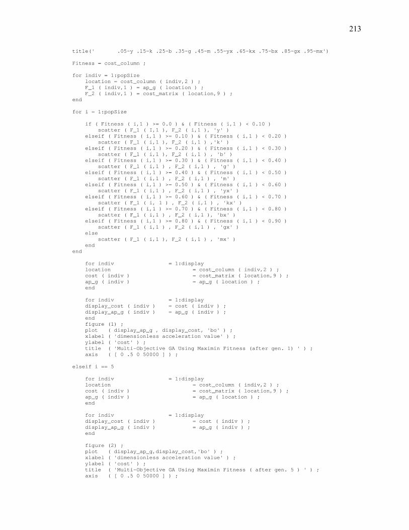
213
title(' .05-y .15-k .25-b .35-g .45-m .55-yx .65-kx .75-bx .85-gx .95-mx') Fitness = cost_column ; for indiv = 1:popSize location = cost_column ( indiv,2 ) ; F_1 ( indiv,1 ) = ap_g ( location ) ; F_2 ( indiv,1 ) = cost_matrix ( location,9 ) ; end for i = 1:popSize if ( Fitness ( i,1 ) >= 0.0 ) & ( Fitness ( i,1 ) < 0.10 ) scatter ( F_1 ( I,1 ), F_2 ( i,1 ), 'y' ) elseif ( Fitness ( i,1 ) >= 0.10 ) & ( Fitness ( i,1 ) < 0.20 ) scatter ( F_1 ( i,1 ), F_2 ( i,1 ) ,'k' ) elseif ( Fitness ( i,1 ) >= 0.20 ) & ( Fitness ( i,1 ) < 0.30 ) scatter ( F_1 ( i,1 ), F_2 ( i,1 ) , 'b' ) elseif ( Fitness ( i,1 ) >= 0.30 ) & ( Fitness ( i,1 ) < 0.40 ) scatter ( F_1 ( i,1 ) , F_2 ( i,1 ) , 'g' ) elseif ( Fitness ( i,1 ) >= 0.40 ) & ( Fitness ( i,1 ) < 0.50 ) scatter ( F_1 ( i,1 ) , F_2 ( i,1 ) , 'm' ) elseif ( Fitness ( i,1 ) >= 0.50 ) & ( Fitness ( i,1 ) < 0.60 ) scatter ( F_1 ( i,1 ) , F_2 ( i,1 ) , 'yx' ) elseif ( Fitness ( i,1 ) >= 0.60 ) & ( Fitness ( i,1 ) < 0.70 ) scatter ( F_1 ( i, 1 ) , F_2 ( i,1 ) , 'kx' ) elseif ( Fitness ( i,1 ) >= 0.70 ) & ( Fitness ( i,1 ) < 0.80 ) scatter ( F_1 ( i,1 ) , F_2 ( i,1 ), 'bx' ) elseif ( Fitness ( i,1 ) >= 0.80 ) & ( Fitness ( i,1 ) < 0.90 ) scatter ( F_1 ( i,1 ) , F_2 ( i,1 ) , 'gx' ) else scatter ( F_1 ( i,1 ), F_2 ( i,1 ) , 'mx' ) end end for indiv = 1:display location = cost_column ( indiv,2 ) ; cost ( indiv ) = cost_matrix ( location,9 ) ; ap_g ( indiv ) = ap_g ( location ) ; end for indiv = 1:display display_cost ( indiv ) = cost ( indiv ) ; display_ap_g ( indiv ) = ap_g ( indiv ) ; end figure (1) ; plot ( display_ap_g , display_cost, 'bo' ) ; xlabel ( 'dimensionless acceleration value' ) ; ylabel ( 'cost' ) ; title ( 'Multi-Objective GA Using Maximin Fitness (after gen. 1) ' ) ; axis ( [ 0 .5 0 50000 ] ) ; elseif i == 5 for indiv = 1:display location = cost_column ( indiv,2 ) ; cost ( indiv ) = cost_matrix ( location,9 ) ; ap_g ( indiv ) = ap_g ( location ) ; end for indiv = 1:display display_cost ( indiv ) = cost ( indiv ) ; display_ap_g ( indiv ) = ap_g ( indiv ) ; end figure (2) ; plot ( display_ap_g,display_cost,'bo' ) ; xlabel ( 'dimensionless acceleration value' ) ; ylabel ( 'cost' ) ; title ( 'Multi-Objective GA Using Maximin Fitness ( after gen. 5 ) ' ) ; axis ( [ 0 .5 0 50000 ] ) ;

214
elseif i == 10 for indiv = 1:display location = cost_column ( indiv,2 ) ; cost ( indiv ) = cost_matrix ( location,9 ) ; ap_g ( indiv ) = ap_g ( location ) ; end for indiv = 1:display display_cost ( indiv ) = cost ( indiv ) ; display_ap_g ( indiv ) = ap_g ( indiv ) ; end figure (3) ; plot ( display_ap_g,display_cost,'bo' ) ; xlabel ( 'dimensionless acceleration value' ) ; ylabel ( 'cost' ) ; title ( 'Multi-Objective GA Using Maximin Fitness ( after gen. 10 ) ' ) ; axis ( [ 0 .5 0 50000 ] ) ; elseif i == 20 for indiv = 1:display location = cost_column ( indiv,2 ) ; cost ( indiv ) = cost_matrix ( location,9 ) ; ap_g ( indiv ) = ap_g ( location ) ; end for indiv = 1:display display_cost ( indiv ) = cost ( indiv ) ; display_ap_g ( indiv ) = ap_g ( indiv ) ; end figure (4) ; plot ( display_ap_g,display_cost,'bo' ) ; xlabel ( 'dimensionless acceleration value' ) ; ylabel ( 'cost' ) ; title ( 'Multi-Objective GA Using Maximin Fitness ( after gen. 20 ) ' ) ; axis ( [ 0 .5 0 50000 ] ) ; elseif i == 30 for indiv = 1:display location = cost_column ( indiv,2 ) ; cost ( indiv ) = cost_matrix ( location,9 ) ; ap_g ( indiv ) = ap_g ( location ) ; end for indiv = 1:display display_cost ( indiv ) = cost ( indiv ) ; display_ap_g ( indiv ) = ap_g ( indiv ) ; end figure (5) ; plot ( display_ap_g,display_cost,'bo' ) ; xlabel ( 'dimensionless acceleration value' ) ; ylabel ( 'cost' ) ; title ( 'Multi-Objective GA Using Maximin Fitness ( after gen. 30 ) ' ) ; axis ( [ 0 .5 0 50000 ] ) ; elseif i == 40 for indiv = 1:display location = cost_column ( indiv,2 ) ; cost ( indiv ) = cost_matrix ( location,9 ) ; ap_g ( indiv ) = ap_g ( location ) ; end for indiv = 1:display display_cost ( indiv ) = cost ( indiv ) ;
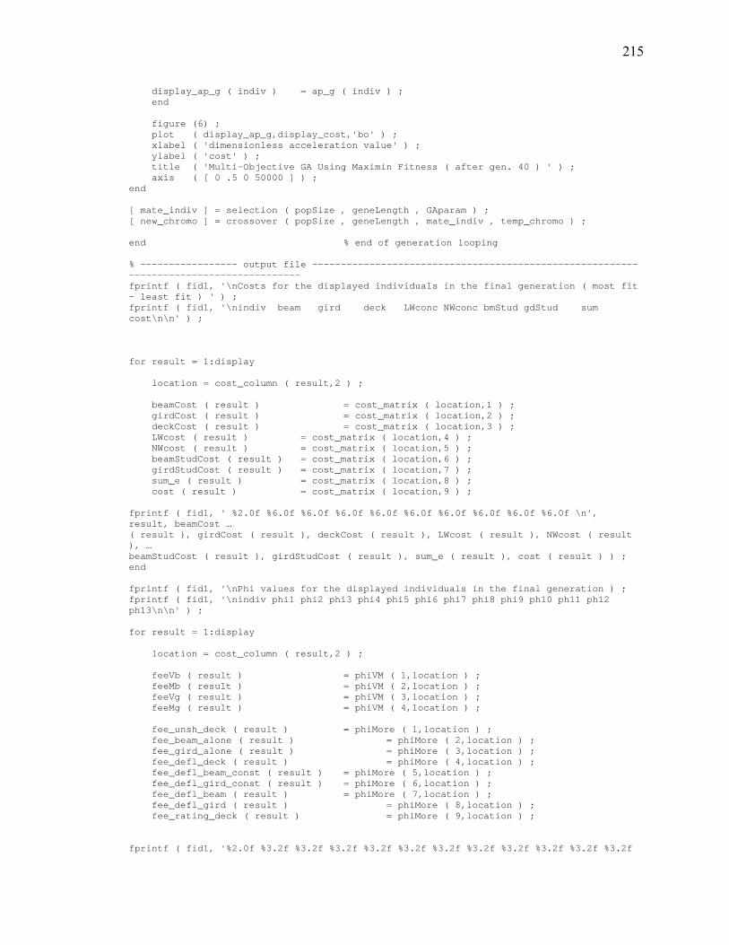
215
display_ap_g ( indiv ) = ap_g ( indiv ) ; end figure (6) ; plot ( display_ap_g,display_cost,'bo' ) ; xlabel ( 'dimensionless acceleration value' ) ; ylabel ( 'cost' ) ; title ( 'Multi-Objective GA Using Maximin Fitness ( after gen. 40 ) ' ) ; axis ( [ 0 .5 0 50000 ] ) ; end [ mate_indiv ] = selection ( popSize , geneLength , GAparam ) ; [ new_chromo ] = crossover ( popSize , geneLength , mate_indiv , temp_chromo ) ; end % end of generation looping % ----------------- output file --------------------------------------------------------------------------------------- fprintf ( fid1, '\nCosts for the displayed individuals in the final generation ( most fit - least fit ) ' ) ; fprintf ( fid1, '\nindiv beam gird deck LWconc NWconc bmStud gdStud sum cost\n\n' ) ; for result = 1:display location = cost_column ( result,2 ) ; beamCost ( result ) = cost_matrix ( location,1 ) ; girdCost ( result ) = cost_matrix ( location,2 ) ; deckCost ( result ) = cost_matrix ( location,3 ) ; LWcost ( result ) = cost_matrix ( location,4 ) ; NWcost ( result ) = cost_matrix ( location,5 ) ; beamStudCost ( result ) = cost_matrix ( location,6 ) ; girdStudCost ( result ) = cost_matrix ( location,7 ) ; sum_e ( result ) = cost_matrix ( location,8 ) ; cost ( result ) = cost_matrix ( location,9 ) ; fprintf ( fid1, ' %2.0f %6.0f %6.0f %6.0f %6.0f %6.0f %6.0f %6.0f %6.0f %6.0f \n', result, beamCost … ( result ), girdCost ( result ), deckCost ( result ), LWcost ( result ), NWcost ( result ), … beamStudCost ( result ), girdStudCost ( result ), sum_e ( result ), cost ( result ) ) ; end fprintf ( fid1, '\nPhi values for the displayed individuals in the final generation ) ; fprintf ( fid1, '\nindiv phi1 phi2 phi3 phi4 phi5 phi6 phi7 phi8 phi9 ph10 ph11 ph12 ph13\n\n' ) ; for result = 1:display location = cost_column ( result,2 ) ; feeVb ( result ) = phiVM ( 1,location ) ; feeMb ( result ) = phiVM ( 2,location ) ; feeVg ( result ) = phiVM ( 3,location ) ; feeMg ( result ) = phiVM ( 4,location ) ; fee_unsh_deck ( result ) = phiMore ( 1,location ) ; fee_beam_alone ( result ) = phiMore ( 2,location ) ; fee_gird_alone ( result ) = phiMore ( 3,location ) ; fee_defl_deck ( result ) = phiMore ( 4,location ) ; fee_defl_beam_const ( result ) = phiMore ( 5,location ) ; fee_defl_gird_const ( result ) = phiMore ( 6,location ) ; fee_defl_beam ( result ) = phiMore ( 7,location ) ; fee_defl_gird ( result ) = phiMore ( 8,location ) ; fee_rating_deck ( result ) = phiMore ( 9,location ) ; fprintf ( fid1, '%2.0f %3.2f %3.2f %3.2f %3.2f %3.2f %3.2f %3.2f %3.2f %3.2f %3.2f %3.2f
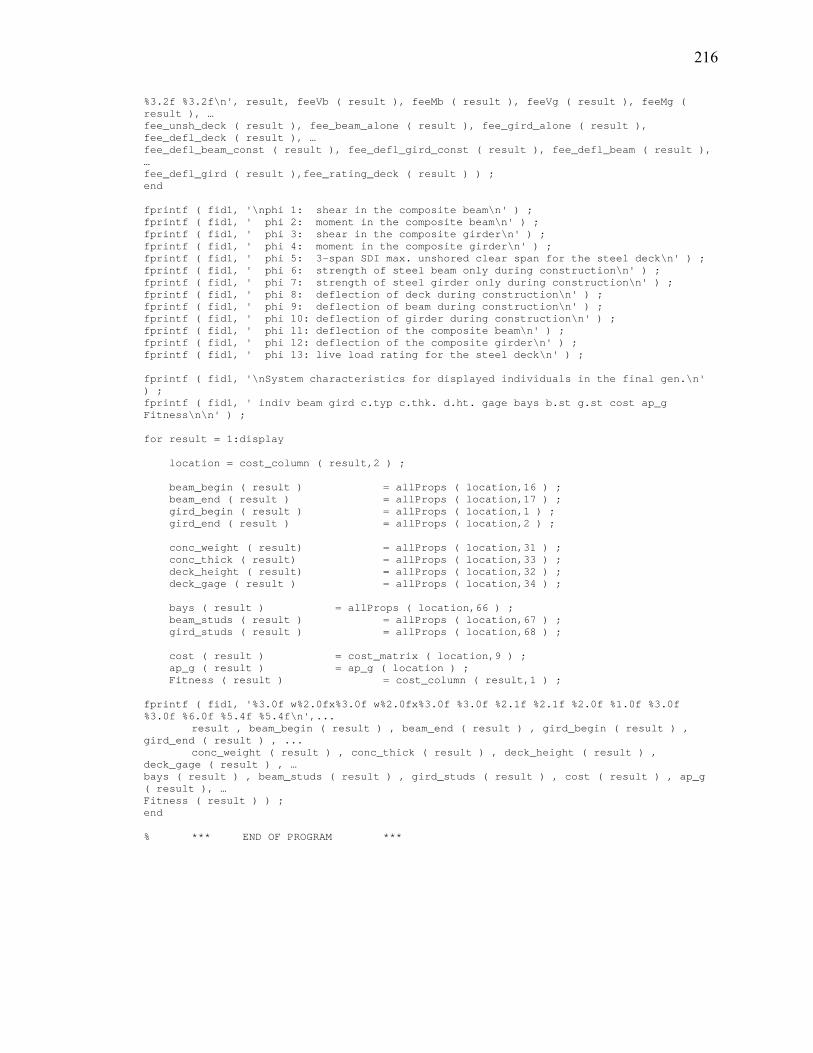
216
%3.2f %3.2f\n', result, feeVb ( result ), feeMb ( result ), feeVg ( result ), feeMg ( result ), … fee_unsh_deck ( result ), fee_beam_alone ( result ), fee_gird_alone ( result ), fee_defl_deck ( result ), … fee_defl_beam_const ( result ), fee_defl_gird_const ( result ), fee_defl_beam ( result ), … fee_defl_gird ( result ),fee_rating_deck ( result ) ) ; end fprintf ( fid1, '\nphi 1: shear in the composite beam\n' ) ; fprintf ( fid1, ' phi 2: moment in the composite beam\n' ) ; fprintf ( fid1, ' phi 3: shear in the composite girder\n' ) ; fprintf ( fid1, ' phi 4: moment in the composite girder\n' ) ; fprintf ( fid1, ' phi 5: 3-span SDI max. unshored clear span for the steel deck\n' ) ; fprintf ( fid1, ' phi 6: strength of steel beam only during construction\n' ) ; fprintf ( fid1, ' phi 7: strength of steel girder only during construction\n' ) ; fprintf ( fid1, ' phi 8: deflection of deck during construction\n' ) ; fprintf ( fid1, ' phi 9: deflection of beam during construction\n' ) ; fprintf ( fid1, ' phi 10: deflection of girder during construction\n' ) ; fprintf ( fid1, ' phi 11: deflection of the composite beam\n' ) ; fprintf ( fid1, ' phi 12: deflection of the composite girder\n' ) ; fprintf ( fid1, ' phi 13: live load rating for the steel deck\n' ) ; fprintf ( fid1, '\nSystem characteristics for displayed individuals in the final gen.\n' ) ; fprintf ( fid1, ' indiv beam gird c.typ c.thk. d.ht. gage bays b.st g.st cost ap_g Fitness\n\n' ) ; for result = 1:display location = cost_column ( result,2 ) ; beam_begin ( result ) = allProps ( location,16 ) ; beam_end ( result ) = allProps ( location,17 ) ; gird_begin ( result ) = allProps ( location,1 ) ; gird_end ( result ) = allProps ( location,2 ) ; conc_weight ( result) = allProps ( location,31 ) ; conc_thick ( result) = allProps ( location,33 ) ; deck_height ( result) = allProps ( location,32 ) ; deck_gage ( result ) = allProps ( location,34 ) ; bays ( result ) = allProps ( location,66 ) ; beam_studs ( result ) = allProps ( location,67 ) ; gird_studs ( result ) = allProps ( location,68 ) ; cost ( result ) = cost_matrix ( location,9 ) ; ap_g ( result ) = ap_g ( location ) ; Fitness ( result ) = cost_column ( result,1 ) ; fprintf ( fid1, '%3.0f w%2.0fx%3.0f w%2.0fx%3.0f %3.0f %2.1f %2.1f %2.0f %1.0f %3.0f %3.0f %6.0f %5.4f %5.4f\n',... result , beam_begin ( result ) , beam_end ( result ) , gird_begin ( result ) , gird_end ( result ) , ... conc_weight ( result ) , conc_thick ( result ) , deck_height ( result ) , deck_gage ( result ) , … bays ( result ) , beam_studs ( result ) , gird_studs ( result ) , cost ( result ) , ap_g ( result ), … Fitness ( result ) ) ; end % *** END OF PROGRAM ***

217
A.7 findFitness.m function [ cost, cost_column, cost_matrix ] = findFitness ( phiProd, phiProd2, costIn, popSize, sysIn, allProps ) % % phiProd ( indiv ) = phiVM ( 1,indiv ) * phiVM ( 2,indiv ) * phiVM ( 3,indiv ) * phiVM ( 4,indiv ) ; % % costIn = [ costSteel, costFab, costDeck, costConc, costLConc, costStud, vibeImport ] % % sysIn = [ W, L, q(1), q(2), comp, desGen, Fy, fc, studDia, fu, studUp ] % % allProps = [ wfGird, wfBeam, stDeck, nBays, nStud, ngStud ] % % totalWt ( indiv ) = wtBeams ( indiv ) + wtGirds ( indiv ) + wtDeck ( indiv ) ; % for indiv = 1:popSize wtBeams = allProps ( indiv,17 ) ; % pounds per foot wtGirds = allProps ( indiv,2 ) ; % pounds per foot wtDeck = allProps ( indiv,38 ) ; % pounds per square foot beamStuds = allProps ( indiv,67 ) ; % number of studs per half beam girdStuds = allProps ( indiv,68 ) ; % number of studs per half girder W = sysIn (1) ; % this will be the length of the girders L = sysIn (2) ; % this will be the length of the beams nBays = allProps ( indiv,66 ) ; % the number of beams will be ( nBays + 1 ) squareFeet = W * L ; % this is the square footage for the system (ft^2) squares = squareFeet / 100 ; % this is the number of squares (100 square feet) % for the system costSteel = costIn (1) ; % this is the cost in dollars per pound of % steel (materials) costFab = costIn (2) ; % this is annother cost in dollars per pound % of steel (fabrication) costDeck = costIn (3) ; % this is a cost in dollars per pound of deck costConc = costIn (4) ; % this is a cost in dollars per cubic yard of % normal-weight concrete costLConc = costIn (5) ; % this is a cost in dollars per cubic yard of % light-weight concrete costStud = costIn (6) ; % this is a cost in dollars per shear stud % (including labor) % Find volume of concrete ------------------------------------------------------------------------------------------- concType = allProps ( indiv,31 ) ; % this will either be 110 or 145 pcf tc = allProps ( indiv,33 ) ; % this is the thickness of the concrete cover ribThick = allProps ( indiv,32 ) ; % this is rib height totalThick = tc + ribThick ; % total thickness (rib + concrete cover) % yardsPerSq is the value from the Vulcraft catalog % yardsOfLW is the value for yards of light-weight % concrete % yardsOfNW is the value for yards of normal-weight
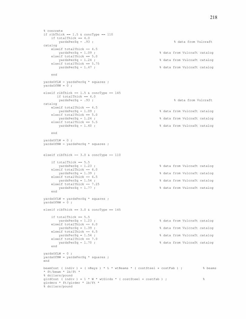
218
% concrete if ribThick == 1.5 & concType == 110 if totalThick == 4.0 yardsPerSq = .93 ; % data from Vulcraft catalog elseif totalThick == 4.5 yardsPerSq = 1.09 ; % data from Vulcraft catalog elseif totalThick == 5.0 yardsPerSq = 1.24 ; % data from Vulcraft catalog elseif totalThick == 5.75 yardsPerSq = 1.47 ; % data from Vulcraft catalog end yardsOfLW = yardsPerSq * squares ; yardsOfNW = 0 ; elseif ribThick == 1.5 & concType == 145 if totalThick == 4.0 yardsPerSq = .93 ; % data from Vulcraft catalog elseif totalThick == 4.5 yardsPerSq = 1.09 ; % data from Vulcraft catalog elseif totalThick == 5.0 yardsPerSq = 1.24 ; % data from Vulcraft catalog elseif totalThick == 5.5 yardsPerSq = 1.40 ; % data from Vulcraft catalog end yardsOfLW = 0 ; yardsOfNW = yardsPerSq * squares ; elseif ribThick == 3.0 & concType == 110 if totalThick == 5.5 yardsPerSq = 1.23 ; % data from Vulcraft catalog elseif totalThick == 6.0 yardsPerSq = 1.39 ; % data from Vulcraft catalog elseif totalThick == 6.5 yardsPerSq = 1.54 ; % data from Vulcraft catalog elseif totalThick == 7.25 yardsPerSq = 1.77 ; % data from Vulcraft catalog end yardsOfLW = yardsPerSq * squares ; yardsOfNW = 0 ; elseif ribThick == 3.0 & concType == 145 if totalThick == 5.5 yardsPerSq = 1.23 ; % data from Vulcraft catalog elseif totalThick == 6.0 yardsPerSq = 1.39 ; % data from Vulcraft catalog elseif totalThick == 6.5 yardsPerSq = 1.54 ; % data from Vulcraft catalog elseif totalThick == 7.0 yardsPerSq = 1.70 ; % data from Vulcraft catalog end yardsOfLW = 0 ; yardsOfNW = yardsPerSq * squares ; end beamCost ( indiv ) = ( nBays ) * L * wtBeams * ( costSteel + costFab ) ; % beams * ft/beam * lb/ft * % dollars/pound girdCost ( indiv ) = 1 * W * wtGirds * ( costSteel + costFab ) ; % girders * ft/girder * lb/ft * % dollars/pound
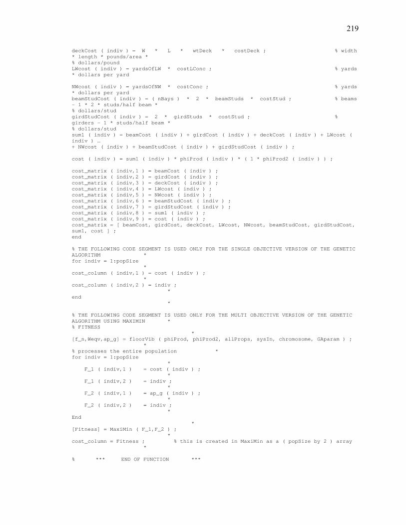
219
deckCost ( indiv ) = W * L * wtDeck * costDeck ; % width * length * pounds/area * % dollars/pound LWcost ( indiv ) = yardsOfLW * costLConc ; % yards * dollars per yard NWcost ( indiv ) = yardsOfNW * costConc ; % yards * dollars per yard beamStudCost ( indiv ) = ( nBays ) * 2 * beamStuds * costStud ; % beams - 1 * 2 * studs/half beam * % dollars/stud girdStudCost ( indiv ) = 2 * girdStuds * costStud ; % girders - 1 * studs/half beam * % dollars/stud sum1 ( indiv ) = beamCost ( indiv ) + girdCost ( indiv ) + deckCost ( indiv ) + LWcost ( indiv ) … + NWcost ( indiv ) + beamStudCost ( indiv ) + girdStudCost ( indiv ) ; cost ( indiv ) = sum1 ( indiv ) * phiProd ( indiv ) * ( 1 * phiProd2 ( indiv ) ) ; cost_matrix ( indiv,1 ) = beamCost ( indiv ) ; cost_matrix ( indiv,2 ) = girdCost ( indiv ) ; cost_matrix ( indiv,3 ) = deckCost ( indiv ) ; cost_matrix ( indiv,4 ) = LWcost ( indiv ) ; cost_matrix ( indiv,5 ) = NWcost ( indiv ) ; cost_matrix ( indiv,6 ) = beamStudCost ( indiv ) ; cost_matrix ( indiv,7 ) = girdStudCost ( indiv ) ; cost_matrix ( indiv,8 ) = sum1 ( indiv ) ; cost_matrix ( indiv,9 ) = cost ( indiv ) ; cost_matrix = [ beamCost, girdCost, deckCost, LWcost, NWcost, beamStudCost, girdStudCost, sum1, cost ] ; end % THE FOLLOWING CODE SEGMENT IS USED ONLY FOR THE SINGLE OBJECTIVE VERSION OF THE GENETIC ALGORITHM * for indiv = 1:popSize * cost_column ( indiv,1 ) = cost ( indiv ) ; * cost_column ( indiv,2 ) = indiv ; * end * % THE FOLLOWING CODE SEGMENT IS USED ONLY FOR THE MULTI OBJECTIVE VERSION OF THE GENETIC ALGORITHM USING MAXIMIN * % FITNESS * [f_n,Weqv,ap_g] = floorVib ( phiProd, phiProd2, allProps, sysIn, chromosome, GAparam ) ; * % processes the entire population * for indiv = 1:popSize * F_1 ( indiv,1 ) = cost ( indiv ) ; * F_1 ( indiv,2 ) = indiv ; * F_2 ( indiv,1 ) = ap_g ( indiv ) ; * F_2 ( indiv,2 ) = indiv ; * End * [Fitness] = MaxiMin ( F_1,F_2 ) ; * cost_column = Fitness ; % this is created in MaxiMin as a ( popSize by 2 ) array * % *** END OF FUNCTION ***
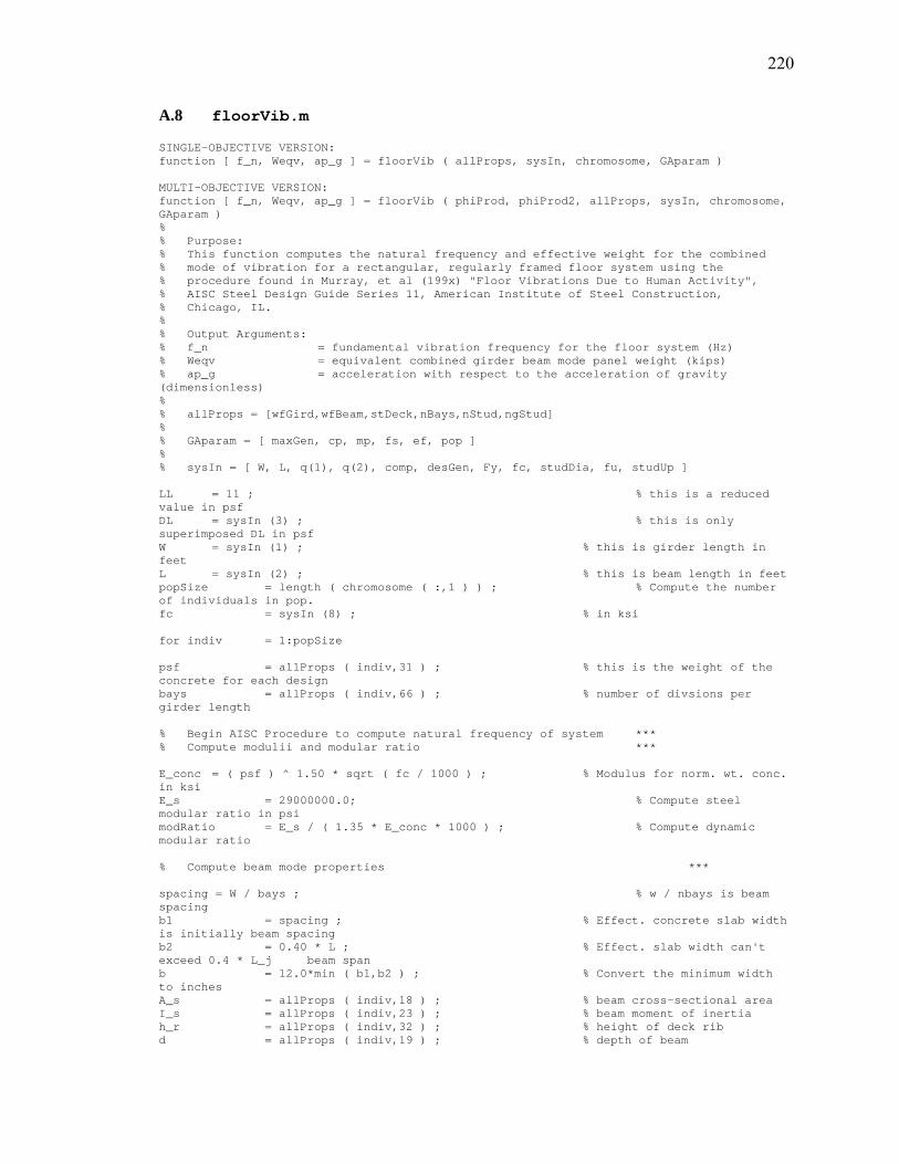
220
A.8 floorVib.m SINGLE-OBJECTIVE VERSION: function [ f_n, Weqv, ap_g ] = floorVib ( allProps, sysIn, chromosome, GAparam ) MULTI-OBJECTIVE VERSION: function [ f_n, Weqv, ap_g ] = floorVib ( phiProd, phiProd2, allProps, sysIn, chromosome, GAparam ) % % Purpose: % This function computes the natural frequency and effective weight for the combined % mode of vibration for a rectangular, regularly framed floor system using the % procedure found in Murray, et al (199x) "Floor Vibrations Due to Human Activity", % AISC Steel Design Guide Series 11, American Institute of Steel Construction, % Chicago, IL. % % Output Arguments: % f_n = fundamental vibration frequency for the floor system (Hz) % Weqv = equivalent combined girder beam mode panel weight (kips) % ap_g = acceleration with respect to the acceleration of gravity (dimensionless) % % allProps = [wfGird,wfBeam,stDeck,nBays,nStud,ngStud] % % GAparam = [ maxGen, cp, mp, fs, ef, pop ] % % sysIn = [ W, L, q(1), q(2), comp, desGen, Fy, fc, studDia, fu, studUp ] LL = 11 ; % this is a reduced value in psf DL = sysIn (3) ; % this is only superimposed DL in psf W = sysIn (1) ; % this is girder length in feet L = sysIn (2) ; % this is beam length in feet popSize = length ( chromosome ( :,1 ) ) ; % Compute the number of individuals in pop. fc = sysIn (8) ; % in ksi for indiv = 1:popSize psf = allProps ( indiv,31 ) ; % this is the weight of the concrete for each design bays = allProps ( indiv,66 ) ; % number of divsions per girder length % Begin AISC Procedure to compute natural frequency of system *** % Compute modulii and modular ratio *** E_conc = ( psf ) ^ 1.50 * sqrt ( fc / 1000 ) ; % Modulus for norm. wt. conc. in ksi E_s = 29000000.0; % Compute steel modular ratio in psi modRatio = E_s / ( 1.35 * E_conc * 1000 ) ; % Compute dynamic modular ratio % Compute beam mode properties *** spacing = W / bays ; % w / nbays is beam spacing b1 = spacing ; % Effect. concrete slab width is initially beam spacing b2 = 0.40 * L ; % Effect. slab width can't exceed 0.4 * L_j beam span b = 12.0*min ( b1,b2 ) ; % Convert the minimum width to inches A_s = allProps ( indiv,18 ) ; % beam cross-sectional area I_s = allProps ( indiv,23 ) ; % beam moment of inertia h_r = allProps ( indiv,32 ) ; % height of deck rib d = allProps ( indiv,19 ) ; % depth of beam

221
a = allProps ( indiv,33 ) ; % height of concrete above rib conc_psf = allProps(indiv,36) ; % weight of concrete in psf deck_psf = allProps(indiv,38) ; % weight of deck in psf beam_plf = allProps(indiv,17) ; % weight of beam in plf yBar = ( A_s * ( h_r + d / 2.0 ) - ( b / modRatio ) * a * ( a / 2.0 ) ) ... / ( A_s + b / modRatio * a ) ; % Centroid depth from deck top I_j = I_s + A_s * ( h_r + d / 2.0 – yBar ) ^ 2 + ( b/ modRatio ) … * ( a ^ 3 ) / 12.0 + ( b / modRatio ) * a * ( yBar + a / 2.0 ) ^ 2 ; % Beam composite moment of inertia w_j = spacing * ( LL + DL + conc_psf + deck_psf )+ beam_plf ; % Unif. distrib. load Delta_j = ( 5.0 * w_j * L ^ 4 ) / ( 384.0 * E_s * I_j ) * 1728.0 ; % Deflection f_j = 0.18 * sqrt ( 386.4 / Delta_j ); % Joist frequency contribution d_e = h_r / 2.0 + a ; % Average concrete thickness A = 12.0 * d_e / modRatio ; % Equivalent area of composite slab D_s = ( 12.0 / modRatio ) * ( d_e ^ 3 / 12.0 ) ; % Transformed moment of inertia % of slab per unit width D_j = I_j / spacing ; % Transformed mom. of iner. % of beam panel per width C_j = 2.0 ; % Assumes beam is interior B1 = ( 2.0 / 3.0 ) * W * 3 ; % THE THREE IS ASSUMING AT % LEAST THREE PANELS B2 = C_j * ( D_s / D_j ) ^ 0.25 * L ; B_j = min ( B1,B2 ) ; % Effective beam panel width W_j = 1.5 * ( w_j / spacing ) * B_j * L ; % Effective weight of beam panel % Compute Girder mode properties *** b1 = 0.40 * W ; % Effect. concrete slab width is initially 0.4*L_g b2 = L ; % Effect. slab width can't exceen L_j b = 12.0*min ( b1,b2 ) ; % Convert to inches A_s = allProps ( indiv,3 ) ; % beam cross-sectional area I_s = allProps ( indiv,8 ) ; % beam moment of inertia h_r = allProps ( indiv,32 ) ; % height of deck rib d = allProps ( indiv,4 ) ; % depth of beam a = allProps ( indiv,33 ) ; % height of concrete above rib acd = a + h_r / 2 ; % average concrete depth gird_plf = allProps(indiv,2) ; % weight of girder yBar = ( A_s * ( h_r / 2 + d / 2.0) - ( b / modRatio ) * acd * … ( acd / 2.0 ) ) / ( A_s + b / modRatio * acd ) ; % Centroid depth from deck top I_g = I_s + A_s * ( h_r / 2 + d / 2.0 – yBar ) ^ 2 + … ( b / modRatio ) * ( acd ^ 3 ) / 12.0 + … ( b / modRatio ) * acd * ( yBar + acd / 2.0 ) ^ 2 ;

222
% Beam composite moment of inertia w_g = L * ( w_j / spacing ) + gird_plf ; % Equivalent girder unif. Load Delta_g = ( 5.0 * w_g * W ^ 4 ) / ( 384.0 * E_s * I_g ) * 1728.0 ; % Deflection f_g = 0.18 * sqrt ( 386.4 / Delta_g ) ; % Girder frequency contribution D_g = I_g/L ; % Girder transformed flexural rigidity per foot C_g = 1.80 ; % Assumes beam connected to girder web B1 = ( 2.0 / 3.0 ) * L * 3 ; % 2/3 times floor length limit % THE THREE IS ASSUMING AT LEAST THREE PANELS B2 = C_g * ( D_j / D_g ) ^ 0.25 * W ; % Actual panel width B_g = min ( B1,B2 ) ; % Effective panel width for girder (ft) W_g = ( w_g / L) * B_g * W ; % Effective weight of girder panel if W < B_j Delta_g = W / B_j * Delta_g ; % Reduce girder deflection accordingly end % Compute vibration parameters of the floor system *** f_n ( indiv ) = 0.18 * sqrt ( 386.4 / ( Delta_j + Delta_g ) ) ; % Fundamental frequency of floor system Weqv ( indiv ) = ( Delta_j / ( Delta_j + Delta_g) ) * W_j ... + ( Delta_g / ( Delta_j + Delta_g) ) * W_g ; % Equivalent combined mode panel weight P_o = 65 ; % Constant Force in lbs. ( AISC Design Guide Series 11, 1997 ) Beta = 0.030 ; % this is an approximate value ( AISC Design Guide Series 11, 1997 ) % this is for floors with non-structural components and furnishings % this is what was used in LAMAN and AISC 11 examples SINGLE-OBJECTIVE VERSION: ap_g ( indiv ) = ( P_o * exp ( -0.35 * f_n ( indiv ) ) ) / ( Beta * Weqv ( indiv ) ) * 100 ; MULTI-OBJECTIVE VERSION: ap_g ( indiv ) = ( P_o * exp ( -0.35 * f_n ( indiv ) ) ) / ( Beta * Weqv ( indiv ) ) * 100 * phiProd(indiv) ... * phiProd2(indiv) ; end % *** END OF FUNCTION ***
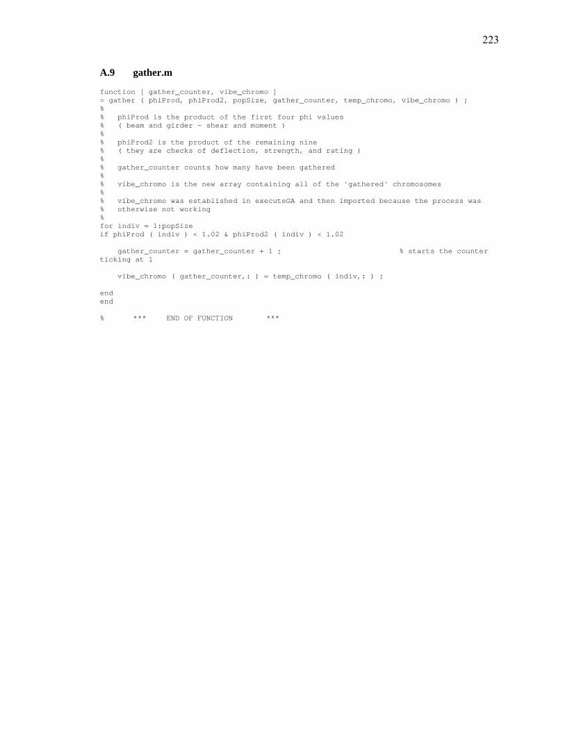
223
A.9 gather.m function [ gather_counter, vibe_chromo ] = gather ( phiProd, phiProd2, popSize, gather_counter, temp_chromo, vibe_chromo ) ; % % phiProd is the product of the first four phi values % ( beam and girder - shear and moment ) % % phiProd2 is the product of the remaining nine % ( they are checks of deflection, strength, and rating ) % % gather_counter counts how many have been gathered % % vibe_chromo is the new array containing all of the 'gathered' chromosomes % % vibe_chromo was established in executeGA and then imported because the process was % otherwise not working % for indiv = 1:popSize if phiProd ( indiv ) < 1.02 & phiProd2 ( indiv ) < 1.02 gather_counter = gather_counter + 1 ; % starts the counter ticking at 1 vibe_chromo ( gather_counter,: ) = temp_chromo ( indiv,: ) ; end end % *** END OF FUNCTION ***

224
A.10 initialPopulation.m function [ chromosome ] = initialPopulation ( popSize, geneLength ) % Purpose: % This function will create an initial population with randomly chosen % characteristics. % % Inputs: % popSize population size (from executeGA.m) % geneLength array of gene lengths for each design variable % (from master.m) % geneLength = [ girdGene, beamGene, ctypGene, dhgtGene, cthkGene, gageGene, baysGene, studGene, stdgGene ] % % Outputs: % chromosome randomly generated chromosomes % unknowns decoded chromosome values % Determine the length of the chromosome ---------------------------------------------------------------------------- chromLength = 0 ; % Initialize for counting numUNKNO = length ( geneLength ) ; % Determine the number of unknowns % For BTS, numUNKNO will always be equal to nine (9) for i = 1:numUNKNO chromLength = chromLength + geneLength (i) ; end % For BTS, this loop has added the total number of binary digits in the chromosome (34) % Create individual chromosome binary digits randomly --------------------------------------------------------------- for indiv = 1:popSize % Loop over the individuals in the population randNum = rand ( 1,chromLength ) ; % Generate an array of random numbers for allele = 1:chromLength % Loop over all alleles in the chromosome if randNum(allele) > 0.5 chromosome ( indiv,allele ) = 1 ; else chromosome ( indiv,allele ) = 0 ; end end end % *** END OF FUNCTION ***
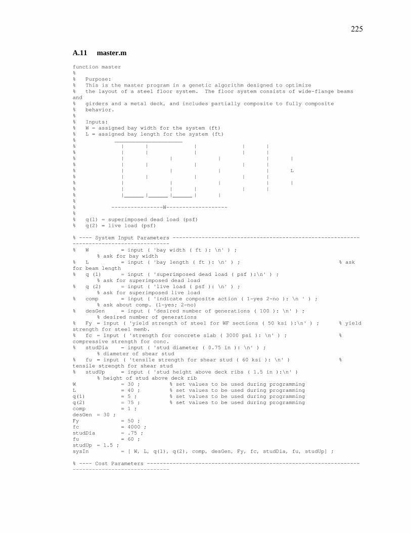
225
A.11 master.m function master % % Purpose: % This is the master program in a genetic algorithm designed to optimize % the layout of a steel floor system. The floor system consists of wide-flange beams and % girders and a metal deck, and includes partially composite to fully composite % behavior. % % Inputs: % W = assigned bay width for the system (ft) % L = assigned bay length for the system (ft) % _____________________ % | | | | | % | | | | | % | | | | | % | | | | | % | | | | L % | | | | | % | | | | | % | | | | | % |______ |______ |______ | | % % ----------------W------------------- % % q(1) = superimposed dead load (psf) % q(2) = live load (psf) % ---- System Input Parameters ---------------------------------------------------------------------------------------- % W = input ( 'bay width ( ft ): \n' ) ; % ask for bay width % L = input ( 'bay length ( ft ): \n' ) ; % ask for beam length % q (1) = input ( 'superimposed dead load ( psf ):\n' ) ; % ask for superimposed dead load % q (2) = input ( 'live load ( psf ): \n' ) ; % ask for superimposed live load % comp = input ( 'indicate composite action ( 1-yes 2-no ): \n ' ) ; % ask about comp. (1-yes; 2-no) % desGen = input ( 'desired number of generations ( 100 ): \n' ) ; % desired number of generations % Fy = input ( 'yield strength of steel for WF sections ( 50 ksi ):\n' ) ; % yield strength for steel memb. % fc = input ( 'strength for concrete slab ( 3000 psi ): \n' ) ; % compressive strength for conc. % studDia = input ( 'stud diameter ( 0.75 in ): \n' ) ; % diameter of shear stud % fu = input ( 'tensile strength for shear stud ( 60 ksi ): \n' ) % tensile strength for shear stud % studUp = input ( 'stud height above deck ribs ( 1.5 in ):\n' ) % height of stud above deck rib W = 30 ; % set values to be used during programming L = 40 ; % set values to be used during programming q(1) = 5 ; % set values to be used during programming q(2) = 75 ; % set values to be used during programming comp = 1 ; desGen = 30 ; Fy = 50 ; fc = 4000 ; studDia = .75 ; fu = 60 ; studUp = 1.5 ; sysIn = [ W, L, q(1), q(2), comp, desGen, Fy, fc, studDia, fu, studUp] ; % ---- Cost Parameters ------------------------------------------------------------------------------------------------
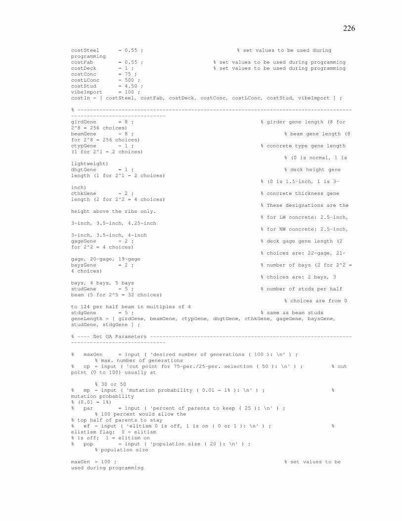
226
costSteel = 0.55 ; % set values to be used during programming costFab = 0.55 ; % set values to be used during programming costDeck = 1 ; % set values to be used during programming costConc = 75 ; costLConc = 500 ; costStud = 4.50 ; vibeImport = 100 ; costIn = [ costSteel, costFab, costDeck, costConc, costLConc, costStud, vibeImport ] ; % --------------------------------------------------------------------------------------------------------------------- girdGene = 8 ; % girder gene length (8 for 2^8 = 256 choices) beamGene = 8 ; % beam gene length (8 for 2^8 = 256 choices) ctypGene = 1 ; % concrete type gene length (1 for 2^1 = 2 choices) % (0 is normal, 1 is lightweight) dhgtGene = 1 ; % deck height gene length (1 for 2^1 = 2 choices) % (0 is 1.5-inch, 1 is 3-inch) cthkGene = 2 ; % concrete thickness gene length (2 for 2^2 = 4 choices) % These designations are the height above the ribs only. % for LW concrete: 2.5-inch, 3-inch, 3.5-inch, 4.25-inch % for NW concrete: 2.5-inch, 3-inch, 3.5-inch, 4-inch gageGene = 2 ; % deck gage gene length (2 for 2^2 = 4 choices) % choices are: 22-gage, 21-gage, 20-gage, 19-gage baysGene = 2 ; % number of bays (2 for 2^2 = 4 choices) % choices are: 2 bays, 3 bays, 4 bays, 5 bays studGene = 5 ; % number of studs per half beam (5 for 2^5 = 32 choices) % choices are from 0 to 124 per half beam in multiples of 4 stdgGene = 5 ; % same as beam studs geneLength = [ girdGene, beamGene, ctypGene, dhgtGene, cthkGene, gageGene, baysGene, studGene, stdgGene ] ; % ---- Set GA Parameters ---------------------------------------------------------------------------------------------- % maxGen = input ( 'desired number of generations ( 100 ): \n' ) ; % max. number of generations % cp = input ( 'cut point for 75-per./25-per. selection ( 50 ): \n' ) ; % cut point (0 to 100) usually at % 30 or 50 % mp = input ( 'mutation probability ( 0.01 = 1% ): \n' ) ; % mutation probability % (0.01 = 1%) % par = input ( 'percent of parents to keep ( 25 ): \n' ) ; % 100 percent would allow the % top half of parents to stay % ef = input ( 'elitism 0 is off, 1 is on ( 0 or 1 ): \n' ) ; % elistism flag: 0 = elitism % is off; 1 = elitism on % pop = input ( 'population size ( 20 ): \n' ) ; % population size maxGen = 100 ; % set values to be used during programming

227
cp = 40 ; % set values to be used during programming mp = 0.015 ; % set values to be used during programming par = 15 ; ef = 1 ; % protects the top (1) choice from mutation % and preserves the top (10) for the next generation pop = 250 ; GAparam = [ maxGen, cp, mp, par, ef, pop] ; % array of GA parameters % ---- Execute GA ----------------------------------------------------------------------------------------------------- executeGA ( geneLength, GAparam, sysIn, costIn ) ; % *** END OF FUNCTION ***
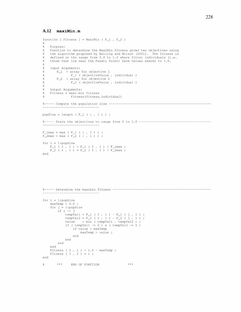
228
A.12 maxiMin.m function [ Fitness ] = MaxiMin ( F_1 , F_2 ) % % Purpose: % Function to determine the MaxiMin fitness given two objectives using % the algorithm proposed by Balling and Wilson (2001). The fitness is % defined on the range from 0.0 to 1.0 where fitter individuals (i.e. % those that lie near the Pareto front) have values nearer to 1.0. % % Input Arguments: % F_1 = array for objective 1 % F_1 ( objectiveValue , individual ) % F_2 = array for objective 2 % F_2 ( objectiveValue , individual ) % % Output Arguments: % Fitness = maxi-min fitness % Fitness(fitness,individual) %----- Compute the population size ------------------------------------------------------------------------------------ popSize = length ( F_1 ( : , 1 ) ) ; %----- Scale the objectives to range from 0 to 1.0 -------------------------------------------------------------------- F_1max = max ( F_1 ( : , 1 ) ) ; F_2max = max ( F_2 ( : , 1 ) ) ; for i = 1:popSize F_1 ( I , 1 ) = F_1 ( I , 1 ) / F_1max ; F_2 ( I , 1 ) = F_2 ( I , 1 ) / F_2max ; end %----- Determine the maximin fitness ---------------------------------------------------------------------------------- for i = 1:popSize maxTemp = 0.0 ; for j = 1:popSize if i ~= j tempVal1 = F_1 ( I , 1 ) - F_1 ( j , 1 ) ; tempVal2 = F_2 ( I , 1 ) - F_2 ( j , 1 ) ; value = min ( tempVal1 , tempVal2 ) ; if ( tempVal1 ~= 0 ) & ( tempVal2 ~= 0 ) if value > maxTemp maxTemp = value ; end end end end Fitness ( I , 1 ) = 1.0 - maxTemp ; Fitness ( I , 2 ) = i ; end % *** END OF FUNCTION ***

229
A.13 moreCheck.m function [ phiMore, defl_beam ] = moreCheck ( sysIn, allProps, popSize, totalWt, ratios ) % This function performs additional checks on strength and deflection states, as well as span ratings, % for construction and end user conditions. % % Outputs: % SINGLE_OBJECTIVE GA: % phiMore = [ unshoredDeck; beamAlone; girdAlone; deflBeamConstr; deflGirdConstr; deflBeam; deflGird; % ratingDeck ] % % SINGLE_OBJECTIVE GA WITH ACCELERATION PENALTY: % phiMore = [ unshoredDeck; beamAlone; girdAlone; accel; deflBeamConstr; deflGirdConstr; deflBeam; deflGird; % ratingDeck ] % % MULTI-OBJECTIVE GA WITH MAXIMIN FITNESS: % phiMore = [ unshoredDeck; beamAlone; girdAlone; deflBeamConstr; deflGirdConstr; deflBeam; deflGird; % ratingDeck ] % % defl_beam is an array of size ( 1 x popSize ) containing deflections % of the composite beam under service LL and s-DL % % Inputs % sysIn = [ W, L, q(1), q(2), comp, desGen, Fy, fc, studDia, fu, studUp ] % allProps = [ wfGird, wfBeam, stDeck, nBays, nStud, ngStud] % totalWt ( indiv ) = wtBeams ( indiv ) + wtGirds ( indiv ) + wtDeck ( indiv ) % % ratios = ( popSize x 2 ) array % consisting of ( beam_ration girder_ratio ) % for each individual in the popululation % % These ratios are used in moreCheck when finding the effective % moment of inertia, Ieff, to be used in calculating the deflection % of the composite beam and girder. Equation (C-I3-6) LRFD 1998 p.6-208. % % Each ratio is: sum Qn / Cf % which is: the strength of the shear connectors between the pointof maximum % positive moment and the point of zero moment divided by the % compression force in the concrete slab for fully composite action. % (the smaller of C-I3-1 and C-I3-2 LRFD 1998 p.6-206. % start by importing the 3-span SDI max. unshored clear span for indiv = 1:popSize threeSpan ( indiv ) = allProps ( indiv,44 ) ; % the 3-span SDI max. unshored clear span W = sysIn (1) ; bays = allProps ( indiv,66 ) ; bf = allProps ( indiv,21 ) ; clearSpan ( indiv ) = ( W / bays ) - ( bf / 12 ) ; % in feet unshoredDeck ( indiv ) = clearSpan ( indiv ) / threeSpan ( indiv ) ; if unshoredDeck ( indiv ) < 1 unshoredDeck ( indiv ) = 1 ; end end % Check strength of steel beams only during construction ----------------------------------------------------------- for indiv = 1:popSize
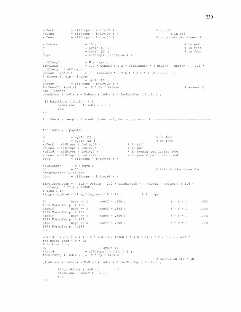
230
wtDeck = allProps ( indiv,38 ) ; % in psf wtConc = allProps ( indiv,36 ) ; % in psf wtBeam = allProps ( indiv,17 ) ; % in pounds per linear foot wtConstr = 10 ; % in psf W = sysIn (1) ; % in feet L = sysIn (2) ; % in feet bays = allProps ( indiv,66 ) ; tribLength = W / bays ; lineLoad = 1.2 * wtBeam + 1.2 * tribLength * ( wtConc + wtDeck ) + 1.6 * tribLength * wtConstr ; MuBeam ( indiv ) = ( ( lineLoad * L * L ) / 8 ) * ( 12 / 1000 ) ; % answer in kip * inches Fy = sysIn (7) ; ZxBeam = allProps ( indiv,26 ) ; facBeamCap (indiv) = .9 * Fy * ZxBeam ; % answer in kip * inches beamAlone ( indiv ) = MuBeam ( indiv ) / facBeamCap ( indiv ) ; if beamAlone ( indiv ) < 1 beamAlone ( indiv ) = 1 ; end end % Check strength of steel girder only during construction ----------------------------------------------------------- for indiv = 1:popSize W = sysIn (1) ; % in feet L = sysIn (2) ; % in feet wtDeck = allProps ( indiv,38 ) ; % in psf wtConc = allProps ( indiv,36 ) ; % in psf wtGird = allProps ( indiv,2 ) ; % in pounds per linear foot wtBeam = allProps ( indiv,17 ) ; % in pounds per linear foot bays = allProps ( indiv,66 ) ; tribLength = W / bays ; LL = 10 ; % this is the value for construction LL in psf bays = allProps ( indiv,66 ) ; line_from_beam = ( 1.2 * wtBeam + 1.2 * tribLength * ( wtDeck + wtConc ) + 1.6 * tribLength * LL ) / 12000 ; % kips / in fac_point_load = line_from_beam * L * 12 ; % in kips if bays == 2 coeff = .250 ; % * P * L LRFD 1998 Formulae p. 4.189 elseif bays == 3 coeff = .333 ; % * P * L LRFD 1998 Formulae p. 4.189 elseif bays == 4 coeff = .500 ; % * P * L LRFD 1998 Formulae p. 4.189 elseif bays == 5 coeff = .600 ; % * P * L LRFD 1998 Formulae p. 4.189 end MuGird ( indiv ) = ( ( 1.2 * wtGird / 12000 ) * ( W * 12 ) ^ 2 / 8 ) + coeff * fac_point_load * W * 12 ; % in kips * in Fy = sysIn (7) ; ZxGird = allProps ( indiv,11 ) ; facGirdCap ( indiv ) = .9 * Fy * ZxGird ; % answer in kip * in girdAlone ( indiv ) = MuGird ( indiv ) / facGirdCap ( indiv ) ; if girdAlone ( indiv ) < 1 girdAlone ( indiv ) = 1 ; end end
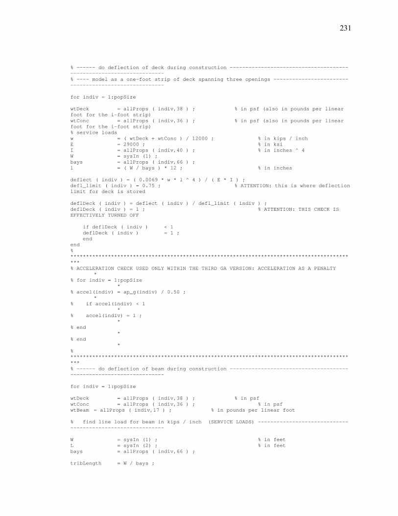
231
% ------ do deflection of deck during construction -------------------------------------------------------------------- % ---- model as a one-foot strip of deck spanning three openings ------------------------------------------------------ for indiv = 1:popSize wtDeck = allProps ( indiv,38 ) ; % in psf (also in pounds per linear foot for the i-foot strip) wtConc = allProps ( indiv,36 ) ; % in psf (also in pounds per linear foot for the i-foot strip) % service loads w = ( wtDeck + wtConc ) / 12000 ; % in kips / inch E = 29000 ; % in ksi I = allProps ( indiv,40 ) ; % in inches ^ 4 W = sysIn (1) ; bays = allProps ( indiv,66 ) ; l = ( W / bays ) * 12 ; % in inches deflect ( indiv ) = ( 0.0069 * w * l ^ 4 ) / ( E * I ) ; defl_limit ( indiv ) = 0.75 ; % ATTENTION: this is where deflection limit for deck is stored deflDeck ( indiv ) = deflect ( indiv ) / defl_limit ( indiv ) ; deflDeck ( indiv ) = 1 ; % ATTENTION: THIS CHECK IS EFFECTIVELY TURNED OFF if deflDeck ( indiv ) < 1 deflDeck ( indiv ) = 1 ; end end % ******************************************************************************************** % ACCELERATION CHECK USED ONLY WITHIN THE THIRD GA VERSION: ACCELERATION AS A PENALTY * % for indiv = 1:popSize * % accel(indiv) = ap_g(indiv) / 0.50 ; * % if accel(indiv) < 1 * % accel(indiv) = 1 ; * % end * % end * % ******************************************************************************************** % ------ do deflection of beam during construction -------------------------------------------------------------------- for indiv = 1:popSize wtDeck = allProps ( indiv,38 ) ; % in psf wtConc = allProps ( indiv,36 ) ; % in psf wtBeam = allProps ( indiv,17 ) ; % in pounds per linear foot % find line load for beam in kips / inch (SERVICE LOADS) ----------------------------------------------------------- W = sysIn (1) ; % in feet L = sysIn (2) ; % in feet bays = allProps ( indiv,66 ) ; tribLength = W / bays ;

232
w = ( tribLength * ( wtConc+wtDeck ) + wtBeam ) / 12000 ; % in kips / inch l = L * 12 ; % in inches E = 29000 ; % in ksi I = allProps ( indiv,23 ) ; % in inches ^ 4 defl_beam ( indiv ) = ( 5 * w * l^4 ) / ( 384 * E * I ) ; % in inches defl_b_limit ( indiv ) = l / 360 ; % in inches deflBeamConstr ( indiv ) = defl_beam ( indiv ) / defl_b_limit ( indiv ) ; if deflBeamConstr ( indiv ) < 1 deflBeamConstr ( indiv ) = 1 ; end end % ------ do deflection of girder during construction ------------------------------------------------------------------ % ------ APPROXIMATED WITH DISTRIBUTED LOAD --------------------------------------------------------------------------- for indiv = 1:popSize wtDeck = allProps ( indiv,38 ) ; % in psf wtConc = allProps ( indiv,36 ) ; % in psf wtGird = allProps ( indiv,2 ) ; % in pounds per linear foot % find line load for girder in kips / inch (SERVICE LOADS) --------------------------------------------------------- W = sysIn (1) ; % in feet L = sysIn (2) ; % in feet tribLength = L ; w = ( tribLength * ( wtConc+wtDeck ) + wtGird ) / 12000 ; % in kips / inch l = W * 12 ; % in inches E = 29000 ; % in ksi I = allProps ( indiv,8 ) ; % in inches ^ 4 defl_gird ( indiv ) = ( 5 * w * l^4 ) / ( 384 * E * I ) ; % in inches defl_g_limit ( indiv ) = l / 360 ; % in inches deflGirdConstr ( indiv ) = defl_gird ( indiv ) / defl_g_limit ( indiv ) ; if deflGirdConstr ( indiv ) < 1 deflGirdConstr ( indiv ) = 1 ; end end % ------ do deflection of composite beam after construction ----------------------------------------------------------- % begin by finding Itr, the moment of inertia for the fully composite uncracked transformed section, in inches ^ 4 for indiv = 1:popSize
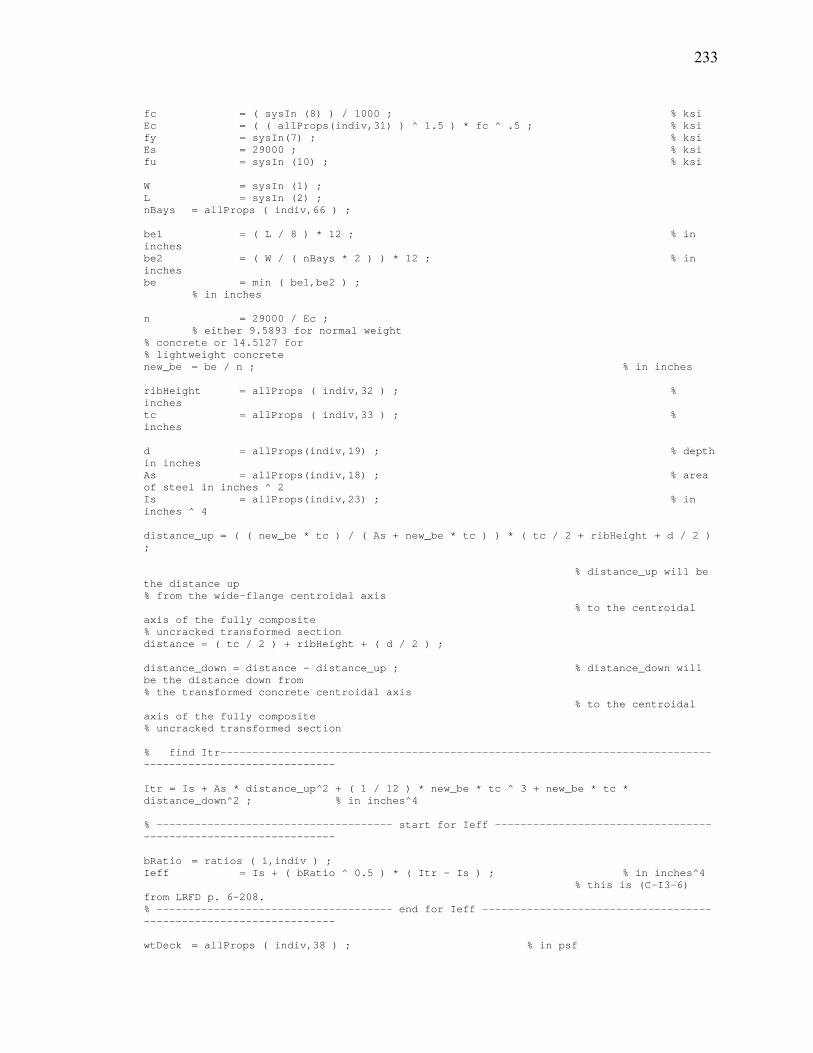
233
fc = ( sysIn (8) ) / 1000 ; % ksi Ec = ( ( allProps(indiv,31) ) ^ 1.5 ) * fc ^ .5 ; % ksi fy = sysIn(7) ; % ksi Es = 29000 ; % ksi fu = sysIn (10) ; % ksi W = sysIn (1) ; L = sysIn (2) ; nBays = allProps ( indiv,66 ) ; be1 = ( L / 8 ) * 12 ; % in inches be2 = ( W / ( nBays * 2 ) ) * 12 ; % in inches be = min ( be1,be2 ) ; % in inches n = 29000 / Ec ; % either 9.5893 for normal weight % concrete or 14.5127 for % lightweight concrete new_be = be / n ; % in inches ribHeight = allProps ( indiv,32 ) ; % inches tc = allProps ( indiv,33 ) ; % inches d = allProps(indiv,19) ; % depth in inches As = allProps(indiv,18) ; % area of steel in inches ^ 2 Is = allProps(indiv,23) ; % in inches ^ 4 distance_up = ( ( new_be * tc ) / ( As + new_be * tc ) ) * ( tc / 2 + ribHeight + d / 2 ) ; % distance_up will be the distance up % from the wide-flange centroidal axis % to the centroidal axis of the fully composite % uncracked transformed section distance = ( tc / 2 ) + ribHeight + ( d / 2 ) ; distance_down = distance - distance_up ; % distance_down will be the distance down from % the transformed concrete centroidal axis % to the centroidal axis of the fully composite % uncracked transformed section % find Itr----------------------------------------------------------------------------------------------------------- Itr = Is + As * distance_up^2 + ( 1 / 12 ) * new_be * tc ^ 3 + new_be * tc * distance_down^2 ; % in inches^4 % ------------------------------------- start for Ieff ---------------------------------------------------------------- bRatio = ratios ( 1,indiv ) ; Ieff = Is + ( bRatio ^ 0.5 ) * ( Itr - Is ) ; % in inches^4 % this is (C-I3-6) from LRFD p. 6-208. % ------------------------------------- end for Ieff ------------------------------------------------------------------ wtDeck = allProps ( indiv,38 ) ; % in psf

234
wtConc = allProps ( indiv,36 ) ; % in psf wtBeam = allProps ( indiv,17 ) ; % in pounds per linear foot % find line load for beam in kips / inch (SERVICE LOADS) ------------------------------------------------------------- W = sysIn (1) ; % in feet L = sysIn (2) ; % in feet bays = allProps ( indiv,66 ) ; DL = sysIn (3) ; % in psf LL = sysIn (4) ; % in psf tribLength = W / bays ; w = ( tribLength * ( DL + LL ) ) / 12000 ; % in kips / inch % *********** LL ONLY *********** l = L * 12 ; % in inches E = 29000 ; % in ksi I = Ieff ; % in inches ^ 4 defl_beam ( indiv ) = ( 5 * w * l ^ 4 ) / ( 384 * E * I ) ; % in inches defl_b_limit ( indiv ) = l / 360 ; % in inches % *** THIS IS WHERE THE BEAM DEFLECTION % LIMIT IS RECORDED*** deflBeam ( indiv ) = defl_beam ( indiv ) / defl_b_limit ( indiv ) ; if deflBeam ( indiv ) < 1 deflBeam ( indiv ) = 1 ; end end % ------ do deflection of composite girder after construction --------------------------------------------------------- % begin by finding Itr, the moment of inertia for the fully composite uncracked transformed section, in inches ^ 4 for indiv = 1:popSize fc = ( sysIn (8) ) / 1000 ; % ksi Ec = ( ( allProps ( indiv,31 ) ) ^ 1.5 ) * fc ^ .5 ; % ksi fy = sysIn (7) ; % ksi Es = 29000 ; % ksi fu = sysIn (10) ; % ksi W = sysIn (1) ; L = sysIn (2) ; be1 = ( W / 8 ) * 12 ; % in inches be2 = ( L / 2 ) * 12 ; % in inches be = min ( be1,be2 ) ; % in inches n = 29000 / Ec ; % either 9.5893 for normal weight concrete % or 14.5127 for lightweight concrete new_be = be / n ; % in inches ribHeight = allProps ( indiv,32 ) ; % inches tc = allProps ( indiv,33 ) ; % inches d = allProps ( indiv,4 ) ; % depth in inches As = allProps ( indiv,3 ) ; % area of steel in inches ^ 2
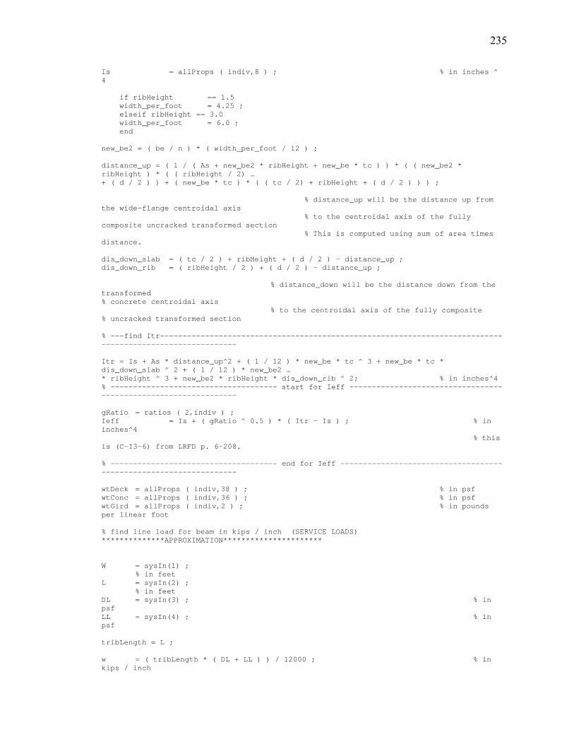
235
Is = allProps ( indiv,8 ) ; % in inches ^ 4 if ribHeight == 1.5 width_per_foot = 4.25 ; elseif ribHeight == 3.0 width_per_foot = 6.0 ; end new_be2 = ( be / n ) * ( width_per_foot / 12 ) ; distance_up = ( 1 / ( As + new_be2 * ribHeight + new_be * tc ) ) * ( ( new_be2 * ribHeight ) * ( ( ribHeight / 2) … + ( d / 2 ) ) + ( new_be * tc ) * ( ( tc / 2) + ribHeight + ( d / 2 ) ) ) ; % distance_up will be the distance up from the wide-flange centroidal axis % to the centroidal axis of the fully composite uncracked transformed section % This is computed using sum of area times distance. dis_down_slab = ( tc / 2 ) + ribHeight + ( d / 2 ) - distance_up ; dis_down_rib = ( ribHeight / 2 ) + ( d / 2 ) - distance_up ; % distance_down will be the distance down from the transformed % concrete centroidal axis % to the centroidal axis of the fully composite % uncracked transformed section % ---find Itr---------------------------------------------------------------------------------------------------------- Itr = Is + As * distance_up^2 + ( 1 / 12 ) * new_be * tc ^ 3 + new_be * tc * dis_down_slab ^ 2 + ( 1 / 12 ) * new_be2 … * ribHeight ^ 3 + new_be2 * ribHeight * dis_down_rib ^ 2; % in inches^4 % ------------------------------------- start for Ieff ---------------------------------------------------------------- gRatio = ratios ( 2,indiv ) ; Ieff = Is + ( gRatio ^ 0.5 ) * ( Itr - Is ) ; % in inches^4 % this is (C-I3-6) from LRFD p. 6-208. % ------------------------------------- end for Ieff ------------------------------------------------------------------ wtDeck = allProps ( indiv,38 ) ; % in psf wtConc = allProps ( indiv,36 ) ; % in psf wtGird = allProps ( indiv,2 ) ; % in pounds per linear foot % find line load for beam in kips / inch (SERVICE LOADS) **************APPROXIMATION********************** W = sysIn(1) ; % in feet L = sysIn(2) ; % in feet DL = sysIn(3) ; % in psf LL = sysIn(4) ; % in psf tribLength = L ; w = ( tribLength * ( DL + LL ) ) / 12000 ; % in kips / inch
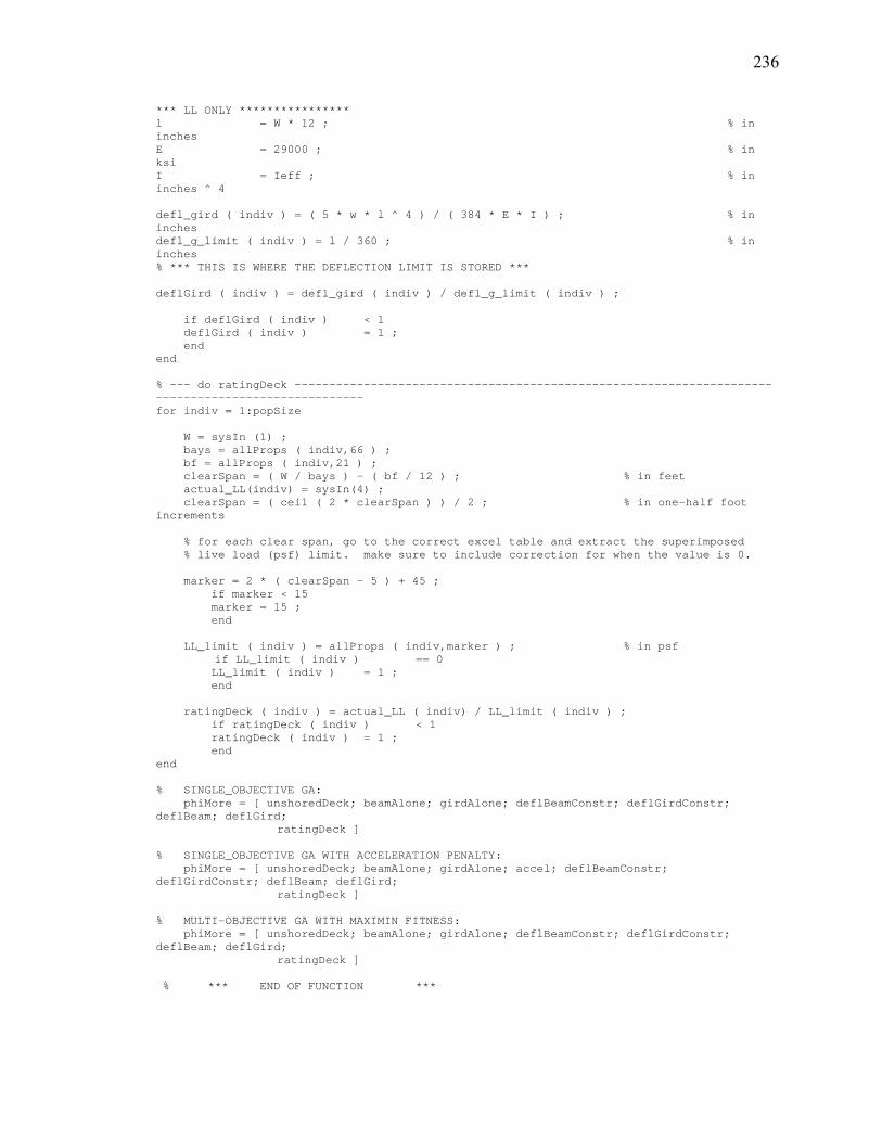
236
*** LL ONLY **************** l = W * 12 ; % in inches E = 29000 ; % in ksi I = Ieff ; % in inches ^ 4 defl_gird ( indiv ) = ( 5 * w * l ^ 4 ) / ( 384 * E * I ) ; % in inches defl_g_limit ( indiv ) = l / 360 ; % in inches % *** THIS IS WHERE THE DEFLECTION LIMIT IS STORED *** deflGird ( indiv ) = defl_gird ( indiv ) / defl_g_limit ( indiv ) ; if deflGird ( indiv ) < 1 deflGird ( indiv ) = 1 ; end end % --- do ratingDeck --------------------------------------------------------------------------------------------------- for indiv = 1:popSize W = sysIn (1) ; bays = allProps ( indiv,66 ) ; bf = allProps ( indiv,21 ) ; clearSpan = ( W / bays ) - ( bf / 12 ) ; % in feet actual_LL(indiv) = sysIn(4) ; clearSpan = ( ceil ( 2 * clearSpan ) ) / 2 ; % in one-half foot increments % for each clear span, go to the correct excel table and extract the superimposed % live load (psf) limit. make sure to include correction for when the value is 0. marker = 2 * ( clearSpan - 5 ) + 45 ; if marker < 15 marker = 15 ; end LL_limit ( indiv ) = allProps ( indiv,marker ) ; % in psf if LL_limit ( indiv ) == 0 LL_limit ( indiv ) = 1 ; end ratingDeck ( indiv ) = actual_LL ( indiv) / LL_limit ( indiv ) ; if ratingDeck ( indiv ) < 1 ratingDeck ( indiv ) = 1 ; end end % SINGLE_OBJECTIVE GA: phiMore = [ unshoredDeck; beamAlone; girdAlone; deflBeamConstr; deflGirdConstr; deflBeam; deflGird; ratingDeck ] % SINGLE_OBJECTIVE GA WITH ACCELERATION PENALTY: phiMore = [ unshoredDeck; beamAlone; girdAlone; accel; deflBeamConstr; deflGirdConstr; deflBeam; deflGird; ratingDeck ] % MULTI-OBJECTIVE GA WITH MAXIMIN FITNESS: phiMore = [ unshoredDeck; beamAlone; girdAlone; deflBeamConstr; deflGirdConstr; deflBeam; deflGird; ratingDeck ] % *** END OF FUNCTION ***

237
A.14 mutation.m function [chromosome] = mutation ( GAparam, chromosome, geneLength, popSize ) % % The array, chromosome, is brought into this function, certain digits are mutated, % and the array is returned to executeGA. % % GAparam = [ maxGen, cp, mp, fs, ef, pop ] % geneLength = [ girdGene, beamGene, ctypGene, dhgtGene, cthkGene, gageGene, baysGene, studGene, stdgGene ] mutation_prob = GAparam (3) ; sum_m = sum ( geneLength ) ; % should be 34 random_mutation = rand ( popSize,sum_m ) ; % ------ elitism ------------------------------------------------------------------------------------------------------ elitism_flag = GAparam (5) ; parents = GAparam (4) ; amount = floor ( ( parents / 200 ) * popSize ) ; marker = popSize – amount + 1 ; if elitism_flag == 1 for digit = 1:sum_m random_mutation ( marker,digit ) = 0.75 ; end end % ------ elitism ------------------------------------------------------------------------------------------------------ for indiv = 1:popSize for digit = 1:sum_m if random_mutation ( indiv,digit ) < mutation_prob if chromosome ( indiv,digit ) == 0 chromosome ( indiv,digit ) = 1 ; else chromosome ( indiv,digit ) = 0 ; end end end end % *** END OF FUNCTION ***
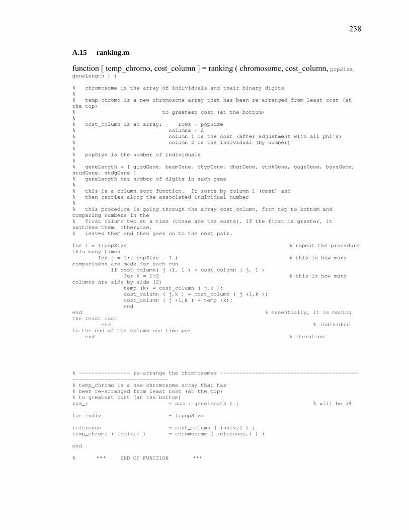
238
A.15 ranking.m function [ temp_chromo, cost_column ] = ranking ( chromosome, cost_column, popSize, geneLength ) ; % chromosome is the array of individuals and their binary digits % % temp_chromo is a new chromosome array that has been re-arranged from least cost (at the top) % to greatest cost (at the bottom) % % cost_column is an array: rows = popSize % columns = 2 % column 1 is the cost (after adjustment with all phi's) % column 2 is the individual (by number) % % popSize is the number of individuals % % geneLength = [ girdGene, beamGene, ctypGene, dhgtGene, cthkGene, gageGene, baysGene, studGene, stdgGene ] % geneLength has number of digits in each gene % % this is a column sort function. It sorts by column 1 (cost) and % then carries along the associated individual number % % this procedure is going through the array cost_column, from top to bottom and comparing numbers in the % first column two at a time (these are the costs). If the first is greater, it switches them, otherwise, % leaves them and then goes on to the next pair. for i = 1:popSize % repeat the procedure this many times for j = 1:( popSize – 1 ) % this is how many comparisons are made for each run if cost_column( j +1, 1 ) < cost_column ( j, 1 ) for k = 1:2 % this is how many columns are side by side (2) temp (k) = cost_column ( j,k ); cost_column ( j,k ) = cost_column ( j +1,k ); cost_column ( j +1,k ) = temp (k); end end % essentially, it is moving the least cost end % individual to the end of the column one time per end % iteration % ---------------- re-arrange the chromosomes ------------------------------------------------------------------------- % temp_chromo is a new chromosome array that has % been re-arranged from least cost (at the top) % to greatest cost (at the bottom) sum_r = sum ( geneLength ) ; % will be 34 for indiv = 1:popSize reference = cost_column ( indiv,2 ) ; temp_chromo ( indiv,: ) = chromosome ( reference,: ) ; end % *** END OF FUNCTION ***
239
A.16 selection.m function [ mate_indiv ] = selection ( popSize, geneLength, GAparam ) % mate_indiv is an array; rows = popSize columns = 3 % columns 1 and 2 are the parents to use for creating the new individual % column 3 is location ( 1 to (34-1) ) where single point crossover will occur % % popSize is the number of individuals % % geneLength = [ girdGene, beamGene, ctypGene, dhgtGene, cthkGene, gageGene, baysGene, studGene, stdgGene] % geneLength has number of digits in each gene % % GAparam = [maxGen,cp,mp,par,ef,pop] ; % cut_point = GAparam (2) ; % usually 40 (75-percent come from top 40-percent) % this means that when selecting two parents to mate, % 75-percent will come from the more-fit group above this cut-off % and 25-percent will come from the less-fit group below the cut. random_matrix = rand ( popSize,5 ) ; % create an array with random numbers % columns 1 and 2 are for parent 1 % columns 3 and 4 are for parent 2 % column 5 is for the location of single-point crossover for indiv = 1:popSize % for the first partner for mating if random_matrix ( indiv,1 ) <= .75 % then we are talking about the top 30 % percent (or number from GAparam(2) ) column_two = random_matrix ( indiv,2 ) ; % holder for the random number which % indicates the individual if column_two == 0 column_two = .0001 ; end % take care of possible zero situation mate_indiv ( indiv,1 ) = ceil ( column_two *… ( cut_point / 100 ) * popSize ) ; else column_two = random_matrix ( indiv,2 ) ; % this is the lower part of the population if column_two == 0 column_two = .0001 ; end mate_indiv ( indiv,1 ) = ceil ( ( cut_point / 100 ) * … popSize + column_two * ( (100-cut_point )… / 100) * popSize ) ; end end for indiv = 1:popSize % for the second partner for mating if random_matrix ( indiv,3 ) <= 0.75 % then we are talking about the top 30 percent % (or number from GAparam(2) ) column_two = random_matrix ( indiv,4 ) ; % holder for the random number which indicates % the individual if column_two == 0 column_two = .0001 ; end % same as above mate_indiv ( indiv,2 ) = ceil ( column_two * … ( cut_point / 100 ) * popSize ) ; % designate mate 2 by number else column_two = random_matrix ( indiv,4 ) ; % same as above if column_two == 0 column_two = .0001 ; end mate_indiv ( indiv,2 ) = ceil ( ( cut_point / 100) … * popSize + column_two * ( (100 - cut_point ) … * / 100) * popSize ) ;
240
end end sum_s = sum( geneLength ) ; % will be 34 for indiv = 1:popSize mate_indiv ( indiv,3 ) = cei l( ( sum_s - 1 ) * random_matrix ( indiv,5 ) ) ; % this establishes the single % point for crossover end % ------ do elitism part. If the elitism flag is on [ GAparam (5) == 1 ] , hold the top ( most-fit ) individuals % ------ and have them return in the new generation. Do this by including the following pairs in % ------ mate_indiv: 1 1 1 % 2 2 1 % 3 3 1 % 4 4 1 % 5 5 1 % --------------------------------------------------------------------------------------------------------------------- elitism_flag = GAparam (5) ; % flag parents = GAparam (4) ; % ( 0 to 100 ) percentage of the population % which becomes number of parents to return amount = floor ( ( parents / 200 ) * popSize ) ; number = 1 ; % this will keep the "most-fit" group of individuals in the current population % it will do so by mating each of the ten best individuals with itself % these couples will form the last "x" lines in the array, mate_indiv if elitism_flag == 1 for line = ( popSize - amount + 1 ):popSize mate_indiv ( line,1 ) = number ; mate_indiv ( line,2 ) = number ; mate_indiv ( line,3 ) = 1 ; number = number + 1 ; end end % *** END OF FUNCTION ***

241
A.17 vmCheck.m function [ phiVM, ratios ] = vmCheck ( sysIn, allProps, popSize, totalWt) % The purpose of this function is to construct the array: % % phiVM = (phiVb;phiMb;phiVg;phiMg) % % where phiXX = factored load / capacity % for the four conditions: % % (1) shear in the beam % (2) moment in the beam % (3) shear in the girder % (4) moment in the girder % % Begin by determining the factored loads that the beam and girder must meet: % based on system inputs: % % sysIn = [ W, L, q(1), q(2), comp, desGen, fy, fc, studDia, fu ] ; % % for each individual (1:popSize), the number of bays is % allProps(indiv,66) % % allProps = [ wfGird, wfBeam, stDeck, nBays, nStud, ngStud] % allProps is of size ( popSize x 68 ) where: % totalWt ( indiv ) = wtBeams ( indiv ) + wtGirds ( indiv ) + wtDeck ( indiv ) ; % --------------------------------------------------------------------------------------------------------------------- for indiv = 1:popSize W = sysIn (1) ; % girder length ( ft ) L = sysIn (2) ; % beam length ( ft ) DL = sysIn (3) ; % superimposed DL ( psf ) LL = sysIn (4) ; % superimposed LL ( psf ) N = allProps ( indiv,66 ) ; % number of bays beam_self_weight = allProps ( indiv,17 ) ; % beam self weight ( plf ) gird_self_weight = allProps ( indiv,2 ) ; % girder self weight ( plf ) conc_psf = allProps ( indiv,36 ) ; % concrete weight ( psf ) deck_psf = allProps ( indiv,38 ) ; % deck weight ( psf ) % begin by finding the factored shear in the beam ------------------------------------------------------------------- % find factored line load on beam: beam_trib = W / N ; % beam tributary width in feet line_beam = ( 1.2 * beam_self_weight + 1.2 * beam_trib * ( DL + conc_psf + deck_psf )… + 1.6 * beam_trib * LL ) / 12000 ; % k/in vMAXb ( indiv ) = ( line_beam * L * 12 ) / 2 ; % kips % find the factored moment in the beam ------------------------------------------------------------------------------ mMAXb(indiv) = ( line_beam * ( L * 12 ) ^ 2 ) / 8 ; % in kips * in

242
% find the factored shear and moment in the girder ------------------------------------------------------------------ fac_point_load = line_beam * L * 12 ; % in kips vMAXg ( indiv ) = ( (N - 1) / 2 ) * fac_point_load + ( ( 1.2 * gird_self_weight * W ) / 2000 ) ; % in kips (works for all N) if N == 2 coeff = .250 ; % * P * L LRFD 1998 Formulae p. 4.189 elseif N == 3 coeff = .333 ; % * P * L LRFD 1998 Formulae p. 4.189 elseif N == 4 coeff = .500 ; % * P * L LRFD 1998 Formulae p. 4.189 elseif N == 5 coeff = .600 ; % * P * L LRFD 1998 Formulae p. 4.189 end % answer in kip * in. mMAXg ( indiv ) = ( ( 1.2 * gird_self_weight / 12000 ) * ( W * 12 ) ^ 2 / 8 )… + coeff * fac_point_load * W * 12 ; % in kip * in end % --------------------------------------------------------------------------------------------------------------------- % This section will be used to develop the facored BEAM % shear and moment capacities of the beam and girder BEAM for indiv = 1:popSize % ---- steel and concrete properties ---------------------------------------------------------------------------------- fc = ( sysIn (8) ) / 1000 ; % ksi Ec = ( ( allProps ( indiv,31 ) ) ^ 1.5 ) * fc ^ .5 ; % ksi fy = sysIn (7) ; % ksi Es = 29000 ; % ksi fu = sysIn (10) ; % ksi % ---- stud properties BEAM -------------------------------------------------------------------------------------- studDia = sysIn(9) ; % inches studArea = ( studDia / 2 ) ^ 2 * 3.14159265 ; % in ^ 2 numStuds = allProps ( indiv, 67 ) ; Qn = 0.5 * studArea * ( fc * Ec ) ^ .5 ; % per stud in kips limit = studArea * fu ; % limit per stud in kips if Qn > limit Qn = limit ; end % ---- find effective width of slab BEAM --------------------------------------------------------------------------- W = sysIn (1) ; L = sysIn (2) ; nBays = allProps ( indiv,66 ) ; be1 = ( L / 8 ) * 12 ; % in inches be2 = ( W / (nBays*2) ) * 12 ; % in inches be = min(be1,be2) ; % in inches % ---- beam data ------------------------------------------------------------------------------------------------------ tw = allProps ( indiv,20 ) ; % web thickness in inches d = allProps ( indiv,19 ) ; % depth in inches As = allProps ( indiv,18 ) ; % area of steel in inches ^ 2 bf = allProps ( indiv,21 ) ; % flange width in inches
243
tf = allProps ( indiv,22 ) ; % thickness of the flange in inches % ---- deck data BEAM ----------------------------------------------------------------------------------------------- ribSpacing = allProps ( indiv,35 ) ; % inches ribHeight = allProps ( indiv,32 ) ; % inches tc = allProps ( indiv,33 ) ; yc = tc + ribHeight ; % ---- stud spacing issues BEAM ------------------------------------------------------------------------------------- numSpots = floor ( L / 2 ) * 2 ; % This is the number of spots per half beam % in the longitudinal direction. It takes into if numStuds > numSpots % account the fact that there are two spots per longitudinal Nr = ceil ( numStuds / numSpots ) ; % direction in the 3-inch deck, but does not include else % 2 or more (buddy) in transverse direction. Nr = 1 ; end if Nr > 3 % I 3-1 LRFD Gray p 6 - 65 Nr = 3 ; end % ---- find R BEAM ------------------------------------------------------------------------------------------------ hr = ribHeight ; if hr == 1.5 wr = 2.125 ; else wr = 6 ; end hs = hr + sysIn(11) ; % The height of a stud will be height of the deck rib plus user input R = ( ( .85 * wr ) / ( ( Nr ^ 0.5) * hr ) ) * ( (hs / hr) - 1 ) ; if R > 1 R = 1 ; end % ---- Shear strength of studs in formed metal decks with ribs perpendicular to beam BEAM --------------------------- Qnr = R * .5 * studArea * ( fc * Ec ) ^ 0.5 ; limitTwo = studArea * fu ; if Qnr > limitTwo Qnr = limitTwo end % ---- shear (V) check for BEAM --------------------------------------------------------------------------------------- BeamVcap ( indiv ) = .9 * tw * d *.6 * fy ; % in kips phiVb ( indiv ) = vMAXb ( indiv ) / BeamVcap ( indiv ) ; if phiVb ( indiv ) < 1.0 phiVb ( indiv ) = 1 ; end % ---- moment (M) check for BEAM -------------------------------------------------------------------------------------- Zx = allProps ( indiv,26 ) ;
244
Mp = Zx * fy ; C_star = .85 * fc * tc * be ; Pyf = bf * tf * fy ; Py = As * fy ; Pyweb = Py - 2 * Pyf ; a = Py / ( .85 * fc * be ) ; if a > tc a = tc ; end y2 = yc - ( a / 2) ; y_bar = ( ( Py - C_star ) / ( 2 * bf * fy ) ) ; z_bar = ( C_star / ( 2 * tw * fy ) ) ; N = allProps ( indiv,67 ) ; % --------------------------------------------------------------------------------------------------------------------- if C_star >= 0 & C_star < Pyweb % then PNA in WEB BEAM % then PNA in WEB BEAM N_full = min ( ( Py / Qnr ) , (C_star / Qnr ) ) ; % then PNA in WEB if N >= N_full % then PNA in WEB BEAM phi_Mn ( indiv ) = .85 * C_star * ( ( d / 2) + y2 ) + … .85 * Mp - .85 * fy * tw * ( ( z_bar ) ^ 2) ; % then PNA in WEB BEAM Qn_defl ( indiv ) = C_star ; % this is the strength of shear connectors C_defl ( indiv ) = C_star ; % this is the C force in the slab for % fully comp. action else % then PNA in WEB BEAM C = N * Qnr ; a = C / ( .85 * fc * be ) ; y2 = yc - (a/2) ; z_bar = ( C / ( 2 * tw * fy ) ) ; % then PNA in WEB phi_Mn ( indiv ) = .85 * C * ( ( d / 2) + y2 ) + .85 * Mp - .85 * fy * tw * ( ( z_bar ) ^ 2 ) ; % answer in k * in Qn_defl ( indiv ) = C ; % this is the strength of shear connectors C_defl ( indiv ) = C_star ; % this is the C force in the slab end % for fully comp. action elseif C_star >= Pyweb & C_star < Py % then PNA in FLANGE BEAM N_full = min ( (Py/Qnr) , (C_star/Qnr) ) ; if N >= N_full phi_Mn ( indiv ) = .85 * C_star * ( ( y_bar / 2) + y2 ) + .85 * Py * ( ( d - y_bar ) / 2 ) ; % answer in k * in Qn_defl ( indiv ) = C_star ; % this is the strength of shear connectors C_defl ( indiv ) = C_star ; % this is the C force in the slab for fully comp. action else
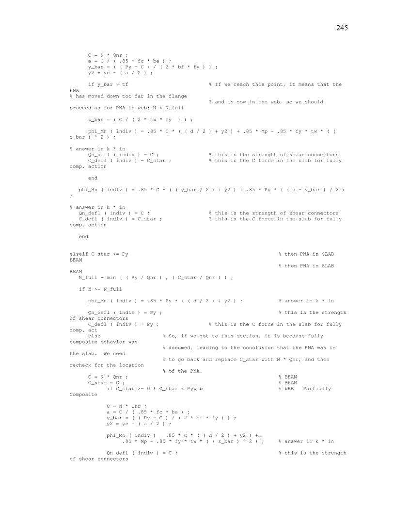
245
C = N * Qnr ; a = C / ( .85 * fc * be ) ; y_bar = ( ( Py - C ) / ( 2 * bf * fy ) ) ; y2 = yc - ( a / 2 ) ; if y_bar > tf % If we reach this point, it means that the PNA % has moved down too far in the flange % and is now in the web, so we should proceed as for PNA in web: N < N_full z_bar = ( C / ( 2 * tw * fy ) ) ; phi_Mn ( indiv ) = .85 * C * ( ( d / 2 ) + y2 ) + .85 * Mp - .85 * fy * tw * ( ( z_bar ) ^ 2 ) ; % answer in k * in Qn_defl ( indiv ) = C ; % this is the strength of shear connectors C_defl ( indiv ) = C_star ; % this is the C force in the slab for fully comp. action end phi_Mn ( indiv ) = .85 * C * ( ( y_bar / 2 ) + y2 ) + .85 * Py * ( ( d - y_bar ) / 2 ) ; % answer in k * in Qn_defl ( indiv ) = C ; % this is the strength of shear connectors C_defl ( indiv ) = C_star ; % this is the C force in the slab for fully comp. action end elseif C_star >= Py % then PNA in SLAB BEAM % then PNA in SLAB BEAM N_full = min ( ( Py / Qnr ) , ( C_star / Qnr ) ) ; if N >= N_full phi_Mn ( indiv ) = .85 * Py * ( ( d / 2 ) + y2 ) ; % answer in k * in Qn_defl ( indiv ) = Py ; % this is the strength of shear connectors C_defl ( indiv ) = Py ; % this is the C force in the slab for fully comp. act else % So, if we got to this section, it is because fully composite behavior was % assumed, leading to the conclusion that the PNA was in the slab. We need % to go back and replace C_star with N * Qnr, and then recheck for the location % of the PNA. C = N * Qnr ; % BEAM C_star = C ; % BEAM if C_star >= 0 & C_star < Pyweb % WEB Partially Composite C = N * Qnr ; a = C / ( .85 * fc * be ) ; y_bar = ( ( Py - C ) / ( 2 * bf * fy ) ) ; y2 = yc - ( a / 2 ) ; phi_Mn ( indiv ) = .85 * C * ( ( d / 2 ) + y2 ) +… .85 * Mp - .85 * fy * tw * ( ( z_bar ) ^ 2 ) ; % answer in k * in Qn_defl ( indiv ) = C ; % this is the strength of shear connectors
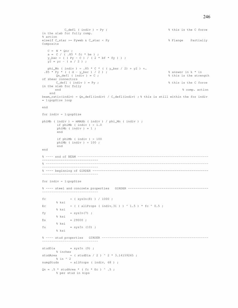
246
C_defl ( indiv ) = Py ; % this is the C force in the slab for fully comp. % action elseif C_star >= Pyweb & C_star < Py % Flange Partially Composite C = N * Qnr ; a = C / ( .85 * fc * be ) ; y_bar = ( ( Py - C ) / ( 2 * bf * fy ) ) ; y2 = yc - ( a / 2 ) ; phi_Mn ( indiv ) = .85 * C * ( ( y_bar / 2) + y2 ) +… .85 * Py * ( ( d - y_bar ) / 2 ) ; % answer in k * in Qn_defl ( indiv ) = C ; % this is the strength of shear connectors C_defl ( indiv ) = Py ; % this is the C force in the slab for fully end % comp. action end beam_ratio(indiv) = Qn_defl(indiv) / C_defl(indiv) ; % this is still within the for indiv = 1:popSize loop end for indiv = 1:popSize phiMb ( indiv ) = mMAXb ( indiv ) / phi_Mn ( indiv ) ; if phiMb ( indiv ) < 1.0 phiMb ( indiv ) = 1 ; end if phiMb ( indiv ) > 100 phiMb ( indiv ) = 100 ; end end % ---- end of BEAM ---------------------------------------------------------------------------------------------------- % --------------------------------------------------------------------------------------------------------------------- % ---- beginning of GIRDER -------------------------------------------------------------------------------------------- for indiv = 1:popSize % ---- steel and concrete properties GIRDER ------------------------------------------------------------------------- fc = ( sysIn(8) ) / 1000 ; % ksi Ec = ( ( allProps ( indiv,31 ) ) ^ 1.5 ) * fc ^ 0.5 ; % ksi fy = sysIn(7) ; % ksi Es = 29000 ; % ksi fu = sysIn (10) ; % ksi % ---- stud properties GIRDER --------------------------------------------------------------------------------------- studDia = sysIn (9) ; % inches studArea = ( studDia / 2 ) ^ 2 * 3.14159265 ; % in ^ 2 numgStuds = allProps ( indiv, 68 ) ; Qn = .5 * studArea * ( fc * Ec ) ^ .5 ; % per stud in kips
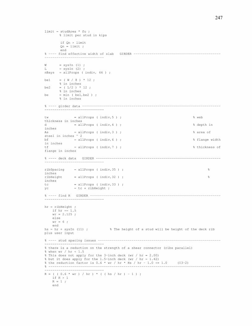
247
limit = studArea * fu ; % limit per stud in kips if Qn > limit Qn = limit ; end % ---- find effective width of slab GIRDER -------------------------------------------------------------------------- W = sysIn (1) ; L = sysIn (2) ; nBays = allProps ( indiv, 66 ) ; be1 = ( W / 8 ) * 12 ; % in inches be2 = ( L/2 ) * 12 ; % in inches be = min ( be1,be2 ) ; % in inches % ---- girder data ---------------------------------------------------------------------------------------------------- tw = allProps ( indiv,5 ) ; % web thickness in inches d = allProps ( indiv,4 ) ; % depth in inches As = allProps ( indiv,3 ) ; % area of steel in inches ^ 2 bf = allProps ( indiv,6 ) ; % flange width in inches tf = allProps ( indiv,7 ) ; % thickness of flange in inches % ---- deck data GIRDER --------------------------------------------------------------------------------------------- ribSpacing = allProps ( indiv,35 ) ; % inches ribHeight = allProps ( indiv,32 ) ; % inches tc = allProps ( indiv,33 ) ; yc = tc + ribHeight ; % ---- find R GIRDER ------------------------------------------------------------------------------------------------ hr = ribHeight ; if hr == 1.5 wr = 2.125 ; else wr = 6 ; end hs = hr + sysIn (11) ; % The height of a stud will be height of the deck rib plus user input % ---- stud spacing issues -------------------------------------------------------------------------------------------- % there is a reduction on the strength of a shear connector (ribs parallel) % when wr / hr < 1.5 % This does not apply for the 3-inch deck (wr / hr = 2.00) % but it does apply for the 1.5-inch deck (wr / hr = 1.42) % the reduction factor is 0.6 * wr / hr * Hs / hr - 1.0 <= 1.0 (I3-2) % --------------------------------------------------------------------------------------------------------------------- R = ( ( 0.6 * wr ) / hr ) * ( ( hs / hr ) - 1 ) ; if R > 1 R = 1 ; end
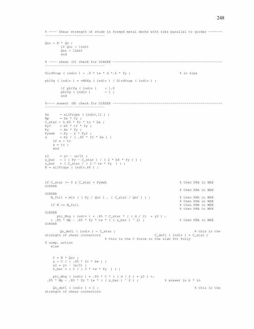
248
% ---- Shear strength of studs in formed metal decks with ribs parallel to girder ------------------------------------- Qnr = R * Qn ; if Qnr > limit Qnr = limit end % ---- shear (V) check for GIRDER ------------------------------------------------------------------------------------- GirdVcap ( indiv ) = .9 * tw * d *.6 * fy ; % in kips phiVg ( indiv ) = vMAXg ( indiv ) / GirdVcap ( indiv ) ; if phiVg ( indiv ) < 1.0 phiVg ( indiv ) = 1 ; end %---- moment (M) check for GIRDER ------------------------------------------------------------------------------------- Zx = allProps ( indiv,11 ) ; Mp = Zx * fy ; C_star = 0.85 * fc * tc * be ; Pyf = bf * tf * fy ; Py = As * fy ; Pyweb = Py - 2 * Pyf ; a = Py / ( .85 * fc * be ) ; if a > tc a = tc ; end y2 = yc - (a/2) ; y_bar = ( ( Py - C_star ) / ( 2 * bf * fy ) ) ; z_bar = ( C_star / ( 2 * tw * fy ) ) ; N = allProps ( indiv,68 ) ; if C_star >= 0 & C_star < Pyweb % then PNA in WEB GIRDER % then PNA in WEB GIRDER N_full = min ( ( Py / Qnr ) , ( C_star / Qnr ) ) ; % then PNA in WEB % then PNA in WEB if N >= N_full % then PNA in WEB % then PNA in WEB GIRDER phi_Mng ( indiv ) = .85 * C_star * ( ( d / 2) + y2 ) … + .85 * Mp - .85 * fy * tw * ( ( z_bar ) ^ 2) ; % then PNA in WEB GIRDER Qn_defl ( indiv ) = C_star ; % this is the strength of shear connectors C_defl ( indiv ) = C_star ; % this is the C force in the slab for fully % comp. action else C = N * Qnr ; a = C / ( .85 * fc * be ) ; y2 = yc - (a/2) ; z_bar = ( C / ( 2 * tw * fy ) ) ; phi_Mng ( indiv ) = .85 * C * ( ( d / 2 ) + y2 ) +… .85 * Mp - .85 * fy * tw * ( ( z_bar ) ^ 2 ) ; % answer in k * in Qn_defl ( indiv ) = C ; % this is the strength of shear connectors
249
C_defl ( indiv ) = C_star ; % this is the C force in the slab for fully % comp. action end elseif C_star >= Pyweb & C_star < Py % then PNA in FLANGE GIRDER N_full = min ( ( Py / Qnr ) , ( C_star / Qnr ) ) ; if N >= N_full phi_Mng ( indiv ) = .85 * C_star * ( ( y_bar / 2) + y2 )… + .85 * Py * ( ( d - y_bar ) / 2 ) ; % answer in k * in Qn_defl ( indiv ) = C_star ; % this is the strength of shear connectors C_defl ( indiv ) = C_star ; % this is the C force in the slab for % fully comp. action else C = N * Qnr ; a = C / ( .85 * fc * be ) ; y_bar = ( ( Py - C ) / ( 2 * bf * fy ) ) ; y2 = yc - ( a / 2 ) ; if y_bar > tf % If we reach this point, it means that the PNA has moved down too far in the flange % and is now in the web, so we should proceed as for PNA in web: N < N_full z_bar = ( C / ( 2 * tw * fy ) ) ; phi_Mng ( indiv ) = .85 * C * ( ( d / 2 ) + y2 ) + .85 * Mp - .85 * fy * tw * ( ( z_bar ) ^ 2 ) ; % answer in k * in Qn_defl ( indiv ) = C ; % this is the strength of shear connectors C_defl ( indiv ) = C_star ; % this is the C force in the slab for fully comp. action end phi_Mng ( indiv ) = .85 * C * ( ( y_bar / 2 ) + y2 ) + .85 * Py * ( ( d - y_bar ) / 2 ) ; % answer in k * in Qn_defl ( indiv ) = C ; % this is the strength of shear connectors C_defl ( indiv ) = C_star ; % this is the C force in the slab for fully comp. action end elseif C_star >= Py % then PNA in SLAB % then PNA in SLAB N_full = min ( ( Py / Qnr ) , ( C_star / Qnr ) ) ; if N >= N_full phi_Mng ( indiv ) = .85 * Py * ( ( d / 2 ) + y2 ) ; % answer in k * in Qn_defl ( indiv ) = Py ; % this is the strength of shear connectors C_defl ( indiv ) = Py ; % this is the C force in the slab for % fully comp. action
250
else % So, if we got to this section, it is because fully composite behavior was % assumed, leading to the conclusion that the PNA was in the slab. We need % to go back and replace C_star with N * Qnr, and then recheck for the location % of the PNA. C = N * Qnr ; % GIRDER C_star = C ; % GIRDER if C_star >= 0 & C_star < Pyweb C = N * Qnr ; a = C / ( .85 * fc * be ) ; y_bar = ( ( Py - C ) / ( 2 * bf * fy ) ) ; y2 = yc - ( a / 2 ) ; phi_Mng ( indiv ) = .85 * C * ( ( d / 2 ) + y2 ) + .85 * Mp - .85 * fy * tw * ( ( z_bar ) ^ 2) ; % answer in k * in Qn_defl ( indiv ) = C ; % this is the strength of shear connectors C_defl ( indiv ) = Py ; % this is the C force in the slab for fully % comp. action elseif C_star >= Pyweb & C_star < Py C = N * Qnr ; a = C / ( .85 * fc * be ) ; y_bar = ( ( Py - C ) / ( 2 * bf * fy ) ) ; y2 = yc - ( a / 2 ) ; phi_Mng ( indiv ) = .85 * C * ( ( y_bar / 2 ) + y2 ) + .85 * Py * ( (d - y_bar) / 2 ) ; % answer in k * in Qn_defl ( indiv ) = C ; % this is the strength of shear connectors C_defl ( indiv ) = Py ; % this is the C force in the slab for % fully comp. action end end gird_ratio ( indiv ) = Qn_defl ( indiv ) / C_defl ( indiv ) ; end for indiv = 1:popSize phiMg ( indiv ) = mMAXg ( indiv ) / phi_Mng ( indiv ) ; if phiMg ( indiv ) < 1.0 phiMg ( indiv ) = 1 ; end if phiMg ( indiv ) > 100 phiMg ( indiv ) = 100 ; end end ratios = [ beam_ratio; gird_ratio ] ; % *** END OF FUNCTION ***

251
Appendix B
Error in Deflection Resulting from
Girder Loading Assumption
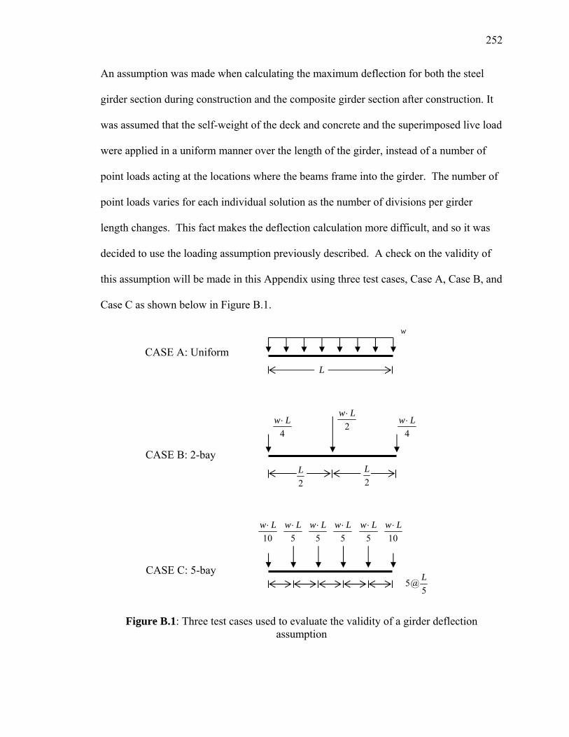
252
An assumption was made when calculating the maximum deflection for both the steel
girder section during construction and the composite girder section after construction. It
was assumed that the self-weight of the deck and concrete and the superimposed live load
were applied in a uniform manner over the length of the girder, instead of a number of
point loads acting at the locations where the beams frame into the girder. The number of
point loads varies for each individual solution as the number of divisions per girder
length changes. This fact makes the deflection calculation more difficult, and so it was
decided to use the loading assumption previously described. A check on the validity of
this assumption will be made in this Appendix using three test cases, Case A, Case B, and
Case C as shown below in Figure B.1.
Figure B.1: Three test cases used to evaluate the validity of a girder deflection assumption
CASE A: Uniform
w
L
CASE B: 2-bay
2L
2L
2w L⋅
4w L⋅
4w L⋅
CASE C: 5-bay 5@
5L
5w L⋅
5w L⋅
5w L⋅
5w L⋅
10w L⋅
10w L⋅

253
Cases A, B, and C all have a total loading of w L⋅ , distributed according to the number of
beams framing into the girder. For Case A, with a uniform loading of w and a beam
length of L, the mid-span deflection is given as,
4 4
max5 0.01302384
w L w LEI EI
δ⎛ ⎞⋅ ⋅ ⋅
= = ⋅⎜ ⎟⋅ ⎝ ⎠ (B.3)
For Case B, with a point load of 2
w L⋅ in the center and a beam length L, the mid-span
deflection is given as,
3
max 48P L
EIδ ⋅
=⋅
(B.4)
where 2
w LP ⋅= , resulting in,
4 4
max 0.0104296w L w L
EI EIδ
⎛ ⎞⋅ ⋅= = ⋅⎜ ⎟⋅ ⎝ ⎠
(B.5)
For Case C, with point loads of 5
w L⋅ and a beam length of L, the mid-span deflection is
given as,
3
maxe P L
EIδ ⋅ ⋅
= (B.6)
where e is given on p. 4-189 of the LRFD Manual (1998) beam tables as 0.063
and5
w LP ⋅= , which results in,
4
max 0.0126 w LEI
δ⎛ ⎞⋅
= ⋅⎜ ⎟⎝ ⎠
(B.7)
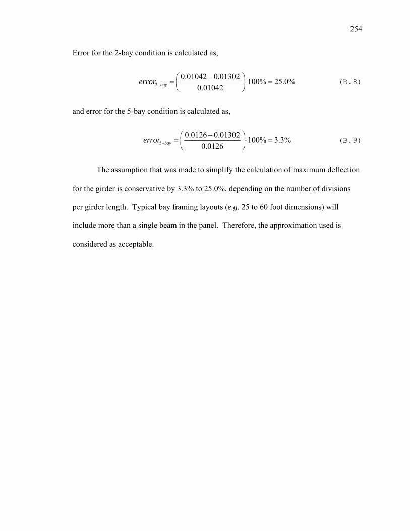
254
Error for the 2-bay condition is calculated as,
20.01042 0.01302 100% 25.0%
0.01042bayerror −
−⎛ ⎞= ⋅ =⎜ ⎟⎝ ⎠
(B.8)
and error for the 5-bay condition is calculated as,
50.0126 0.01302 100% 3.3%
0.0126bayerror −
−⎛ ⎞= ⋅ =⎜ ⎟⎝ ⎠
(B.9)
The assumption that was made to simplify the calculation of maximum deflection
for the girder is conservative by 3.3% to 25.0%, depending on the number of divisions
per girder length. Typical bay framing layouts (e.g. 25 to 60 foot dimensions) will
include more than a single beam in the panel. Therefore, the approximation used is
considered as acceptable.

255
Marquette University
This is to certify that we have examined this copy of the master’s thesis by
Benjamin T. Shock
And have found that it is complete and satisfactory in all respects.
The thesis has been approved by: _____________________________________ Dr. Christopher M. Foley, Department of Civil and Environmental Engineering _____________________________________ Dr. Sriramulu Vinnakota, Department of Civil and Environmental Engineering _____________________________________ Dr. Stephen M. Heinrich, Department of Civil and Environmental Engineering
Approved on: