automated designation of tie-points for image-to-image...
TRANSCRIPT
. . , 2003, . 24, . 17, 3467–3490
Automated designation of tie-points for image-to-image coregistration
R. E. KENNEDY
Department of Forest Science, 321 Richardson Hall, Oregon State University,Corvallis, OR 97331, USA; e-mail: [email protected]
and W. B. COHEN
USDA Forest Service, Pacific Northwest Research Station, Forestry SciencesLaboratory, Corvallis, OR 9733, USA; e-mail: [email protected]
(Received 3 May 2001; in final form 13 June 2002 )
Abstract. Image-to-image registration requires identification of common pointsin both images (image tie-points; ITPs). Here, we describe software implementingan automated, area-based technique for identifying ITPs. The ITP software wasdesigned to follow two strategies: (1) capitalize on human knowledge and pattern-recognition strengths, and (2) favour robustness in many situations over optimalperformance in any one situation. We tested the software under several con-founding conditions, representing image distortions, inaccurate user input, andchanges between images. The software was robust to additive noise, moderatechange between images, low levels of image geometric distortion, undocumentedrotation, and inaccurate pixel size designation. At higher levels of image geometricdistortion, the software was less robust, but such conditions are often visible tothe eye. Methods are discussed for adjusting parameters in the ITP software toreduce error under such conditions. For more than 1600 tests, median time neededto identify each ITP was approximately 8 s on a common image-processingcomputer system. Although correlation-based techniques—such as those imple-mented in the free software documented here—have been criticized, we suggestthat they may, in fact, be quite useful in many situations for users in the remotesensing community.
1. IntroductionWhen two images of the same area are to be analysed, they must be geometrically
registered to one another. Image-to-image registration involves: (1) the identificationof many image tie-points (ITPs), followed by (2) a calculation based on thosepoints for transforming one image’s pixel coordinates into the coordinate space ofthe other image, followed finally by (3) a resampling based on that transformation.While steps 2 and 3 are relatively standardized processes, the manual identificationof image tie-points may be time-consuming and expensive, and includes bias of theinterpreter. For these reasons, automated techniques for detection of ITPs have beendeveloped that are potentially cheaper and repeatable.
The variety of automated registration techniques has been amply summarizedelsewhere (Bernstein 1983, Brown 1992, Fonseca and Manjunath 1996, Schowengerdt1997). Briefly, the techniques to identify tie-points in two images fall into two main
International Journal of Remote SensingISSN 0143-1161 print/ISSN 1366-5901 online © 2003 Taylor & Francis Ltd
http://www.tandf.co.uk/journalsDOI: 10.1080/0143116021000024249
R. E. Kennedy and W. B. Cohen3468
categories: area-based matching and feature-based matching. Area-based matchingapproaches compare spatial patterns of pixel grey-scale values (digital numbers) insmall image subsets (Pratt 1974, Davis and Kenue 1978). Match-points betweenimage subsets are located by maximizing some function of similarity between animage subset in one image and the image subset in another image. The function ofsimilarity may be a modified difference function or a more complex correlationfunction (Bernstein 1983, Schowengerdt 1997). Variations on this basic theme existthat seek to decrease computation time (Barnea and Silverman 1972) or to computea simultaneous solution for multiple points, rather than using sequential imagesubsets (Rosenholm 1987, Li 1991). In contrast to area-based matching, feature-based matching does not attempt to directly match grey-scale pixel patterns betweenthe two images. Rather, pattern-recognition algorithms are applied to grey-scalepixel patterns within each image separately to identify prominent spatial features,such as edges (Davis and Kenue 1978, Li et al. 1995) or unique shapes (Tseng et al.1997). These features are described in terms of shape or pattern parameters that areindependent of the image grey-scale values (Goshtasby et al. 1986, Tseng et al. 1997).The separate features in the two images are then matched based on those shape andpattern parameters.
Although these techniques have been in existence for decades and are well-documented in image-processing texts (Pratt 1991, Schowengerdt 1997), many usersof satellite data still rely on manual designation of tie-points. To assess use ofautomated techniques, we surveyed every article published in the InternationalJournal of Remote Sensing for the year 2001 (i.e. all of volume 22, not including theshorter communications in the L etters section). Of 206 articles surveyed, 59 includedmethodology that required co-registering of images, and thus could have benefitedfrom the use of an automated approach. Only five of those (~8%) used some typeof automated approach for locating ITPs, while 24 (~40%) appeared to use manualco-location of points (table 1). Another 13 studies (~22%) stated that theyco-registered images, but provided no detail how they did so. However, we inferfrom the lack of attention paid to describing geo-registration methodology that mostor all of these studies did not use techniques other than the traditional manualapproach. Thus, it appears likely that over 60% of the studies used manual ITPidentification, while fewer than 10% of the studies used an automated approach.The remaining 30% of the studies manually registered both images to a commonsystem, which is another situation where automated approaches could have beenused. In all, more than 90% of the studies that could have used automated techniquesdid not.
Table 1. Tallies of International Journal of Remote Sensing 2001 articles that co-registeredimages, broken down by the method used to identify ITPs.
Image co-registration method Number of papers
Images separately registered to common system 17Manual ITP selection 12Manual ITP selection inferred, but not explicitly stated 12Automated approach 5Method not stated 13
Total 59
Image-to-image coregistration 3469
The cause for this avoidance of automated techniques is unclear. Certainly,reviews of automated techniques have stressed the weaknesses of both categories ofautomated tie-point designation. Area-based methods require significant computertime (Barnea and Silverman 1972), may only deal with translational offsets (Pratt1974), and may not be useful for data fusion between optical and non-optical sensors(Rignot et al. 1991, Li et al. 1995). Feature-based methods require the existence ofrobust features that are relatively invariant between images, and also require use ofsophisticated feature-extraction algorithms (Fonseca and Manjunath 1996). Fromthe perspective of an applied user of satellite data, it may appear that the automateddetection of tie-points holds more risk than potential reward.
We suggest that many applied users of remote sensing data could benefit from asimple automated approach. In this paper, we describe a publicly-available softwarepackage we have developed that uses a simple area-based approach for automateddetection of image tie-points. We base the software on two strategies: (1) capitalizeon user knowledge and pattern recognition ability, and (2) favour robustness to avariety of image conditions over optimality in any one condition. The former strategyeliminates the greatest unknowns and the costliest components of automated image-matching. The latter relies on the high speed of today’s computers to overcome thetime-consumption of the area-based approach. In addition to describing the software,we report on tests designed to characterize its usefulness under a range of potentiallylimiting conditions.
2. Methods2.1. Automated location of tie-points
Locating each tie-point is a three-step process. In the first step, an approximatetie-point pair is defined in the two images. The approximate tie-point pair is fed tothe area-based correlation module that derives the precise image tie-point pair.Finally, the new pair is validated. The next cycle begins by referring to the positionof the previous tie-point pair.
Step 1: L ocating approximate tie-point pairs. For each image pair, the user suppliesthe coordinates of the first approximate tie-point pair. This simple user input followsthe strategy of capitalizing on human input. The match need not be a true imagetie-point, only an approximation to seed the process (see section 4.7 for a briefdiscussion of this strategy). After the first image tie-point is found and validated(Steps 2 and 3 below), the program automatically locates the second and all sub-sequent approximate tie-point pairs along a regular grid pattern, working systematic-ally left to right and up to down within the images. The spacing of the grid isadjustable.
For the grids to be scaled properly, the true pixel size (pixel-centre to pixel-centredistance on the ground) of each image must be known, as well as the rotation ofthe images relative to each other. The user supplies both of these values. Tests ofthe sensitivity of the process to errors in these estimates are described in section 2.2.Again, the rationale for requiring this user input is based on the strategy of capitaliz-ing on human strengths: the human user likely knows this basic informationabout the two images, and even if these two values are not already known, they canbe approximated easily from simple trigonometry. This is far more efficient thandesigning an iterative procedure to derive these values automatically under any setof circumstances.
R. E. Kennedy and W. B. Cohen3470
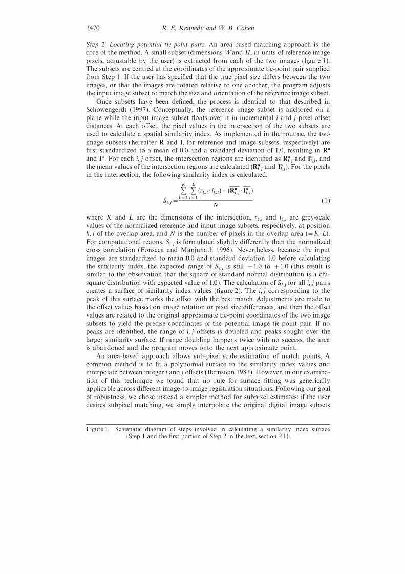
Step 2: L ocating potential tie-point pairs. An area-based matching approach is thecore of the method. A small subset (dimensions W and H, in units of reference imagepixels, adjustable by the user) is extracted from each of the two images (figure 1).The subsets are centred at the coordinates of the approximate tie-point pair suppliedfrom Step 1. If the user has specified that the true pixel size differs between the twoimages, or that the images are rotated relative to one another, the program adjuststhe input image subset to match the size and orientation of the reference image subset.
Once subsets have been defined, the process is identical to that described inSchowengerdt (1997). Conceptually, the reference image subset is anchored on aplane while the input image subset floats over it in incremental i and j pixel offsetdistances. At each offset, the pixel values in the intersection of the two subsets areused to calculate a spatial similarity index. As implemented in the routine, the twoimage subsets (hereafter R and I, for reference and image subsets, respectively) arefirst standardized to a mean of 0.0 and a standard deviation of 1.0, resulting in Rnand In . For each i, j offset, the intersection regions are identified as Rn
i,j and Ini,j , and
the mean values of the intersection regions are calculated (Rni,j and In
i,j ). For the pixelsin the intersection, the following similarity index is calculated:
Si,j=
∑K
k=1∑L
l=1(rk,l · ik,l )−(Rn
i,j · Ini,j )
N(1)
where K and L are the dimensions of the intersection, rk,l and i
k,l are grey-scalevalues of the normalized reference and input image subsets, respectively, at positionk, l of the overlap area, and N is the number of pixels in the overlap area (=K·L ).For computational reaons, S
i,j is formulated slightly differently than the normalizedcross correlation (Fonseca and Manjunath 1996). Nevertheless, because the inputimages are standardized to mean 0.0 and standard deviation 1.0 before calculatingthe similarity index, the expected range of S
i,j is still −1.0 to +1.0 (this result issimilar to the observation that the square of standard normal distribution is a chi-square distribution with expected value of 1.0). The calculation of S
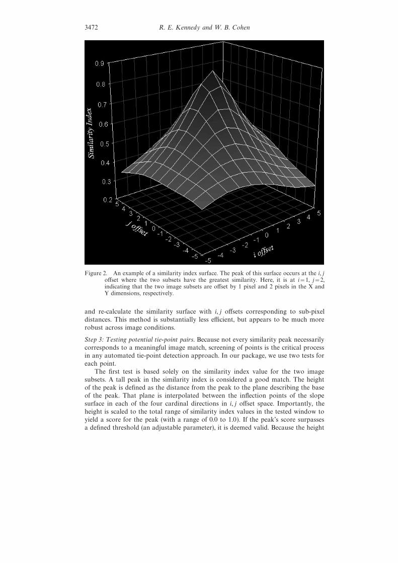
i,j for all i, j pairscreates a surface of similarity index values (figure 2). The i, j corresponding to thepeak of this surface marks the offset with the best match. Adjustments are made tothe offset values based on image rotation or pixel size differences, and then the offsetvalues are related to the original approximate tie-point coordinates of the two imagesubsets to yield the precise coordinates of the potential image tie-point pair. If nopeaks are identified, the range of i, j offsets is doubled and peaks sought over thelarger similarity surface. If range doubling happens twice with no success, the areais abandoned and the program moves onto the next approximate point.
An area-based approach allows sub-pixel scale estimation of match points. Acommon method is to fit a polynomial surface to the similarity index values andinterpolate between integer i and j offsets (Bernstein 1983). However, in our examina-tion of this technique we found that no rule for surface fitting was genericallyapplicable across different image-to-image registration situations. Following our goalof robustness, we chose instead a simpler method for subpixel estimates: if the userdesires subpixel matching, we simply interpolate the original digital image subsets
Figure 1. Schematic diagram of steps involved in calculating a similarity index surface(Step 1 and the first portion of Step 2 in the text, section 2.1).
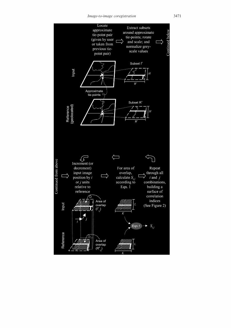
Image-to-image coregistration 3471
R. E. Kennedy and W. B. Cohen3472
Figure 2. An example of a similarity index surface. The peak of this surface occurs at the i, joffset where the two subsets have the greatest similarity. Here, it is at i=1, j=2,indicating that the two image subsets are offset by 1 pixel and 2 pixels in the X andY dimensions, respectively.
and re-calculate the similarity surface with i, j offsets corresponding to sub-pixeldistances. This method is substantially less efficient, but appears to be much morerobust across image conditions.
Step 3: T esting potential tie-point pairs. Because not every similarity peak necessarilycorresponds to a meaningful image match, screening of points is the critical processin any automated tie-point detection approach. In our package, we use two tests foreach point.
The first test is based solely on the similarity index value for the two imagesubsets. A tall peak in the similarity index is considered a good match. The heightof the peak is defined as the distance from the peak to the plane describing the baseof the peak. That plane is interpolated between the inflection points of the slopesurface in each of the four cardinal directions in i, j offset space. Importantly, theheight is scaled to the total range of similarity index values in the tested window toyield a score for the peak (with a range of 0.0 to 1.0). If the peak’s score surpassesa defined threshold (an adjustable parameter), it is deemed valid. Because the height
Image-to-image coregistration 3473
of the peak is scaled to the values observed in each subset image, a general thresholdcan be used that appears to be robust for many different image conditions. If twoor more peaks are determined to be valid with this test, the highest peak is acceptedonly if it exceeds the second-highest peak by a determined proportion. Based on thei, j offset of the peak, the coordinates of the image tie-points are calculated and asecond test is performed.
The second test is based on the relationship between the newly-matched pointand the body of existing tie-points. The distance between any two tie-points can bemeasured either in input image pixel counts, or in reference image map units.Dividing the former distance by the latter distance yields a quantity we refer to asthe pixel size ratio. Unless there is severe distortion in one image, this ratio shouldbe relatively similar across all tie-point pairs. For the second test, then, we estimatethis ratio using only pairs involving the new point and compare that to the estimateusing only pairs without the new point. If the comparison suggests that the newpoint is not from the same population (as determined by a user-alterable threshold),the point is discarded. Note that this second validity test can only be performedwhen a large enough sample of pre-existing image tie-points has been built, and thuscannot be applied to the first few image tie-points located by the methodology. Inevery run of the software reported in section 2.2, the second validity test was onlyused once 10 pairs of tie-points had accumulated.
Although the double-testing process screens out most poor ITPs, a low percentageof sub-optimal pairs may still persist. Before a final matrix of polynomial transforma-tion coefficients is calculated from the points, human screening is advised as a lastcheck. An initial model for the geometric projection solution is calculated andpositional error calculated for all points. Those points with unusually high contribu-tions to the error of the model should be investigated to determine if they areblatantly incorrect and should be screened. As described in section 2.2, it is alsopossible to automate this screening process.
Both the ITP software and the testing software were written in IDL v5.2 (ResearchSystems, Inc., Boulder, CO). They are available at ftp://ftp.fsl.orst.edu/pub/gisdata/larse/itpfind.tar.gz.
2.2. Method for evaluating the ITP location softwareIdeally, the above procedure should be capable of locating ITPs on image pairs
when there are several confounding factors. Broadly, those factors are: (1) the imagesare geometrically distorted relative to each other; (2) image metadata supplied bythe user is not perfectly accurate; and (3) some parts of the images are obscured byclouds or have changed. To evaluate the influence of these factors, we developed aprocedure to quantify error in the ITP process run on any image-to-image pair. Wecould then apply a confounding factor to an image pair, run the ITP software, anddetermine error. By repeating this across many levels of confounding factors, wewere able to build a general evaluation of the conditions under which the softwarewas appropriate.
The procedure to quantify error in a single image pair had three steps. In thefirst, an input image was created from a reference image. Reference images from fivedifferent landscapes were used, as described in section 2.2.1 below. Reference imageswere 601 by 601 pixels in size. Input images were created by projecting the referenceimage with a polynomial transformation coefficient matrix and resampling with anearest-neighbour rule. By creating the input image from the reference image, we

R. E. Kennedy and W. B. Cohen3474
were able to strictly control the types of confounding factors present in the matchingprocess. Geometric distortions were applied by appropriate alteration of the trans-formation matrix prior to resampling. Landscape changes and cloud effects weresimulated by replacing portions of the input image with randomly-placed solid disksof known density, size, and grey-scale value. Simulated inaccuracies in imagemetadata were passed to the ITP process along with the input image.
The second testing step involved running the automated ITP process to locateITPs and then deriving a transformation matrix from those points. For this research,the subset image size was set to 60 reference pixels, with spacing of 80 referencepixels between points, resulting in a grid with a maximum of 60 ITP pairs. Tofacilitate the large number of tests, the human post-processing screen was replacedwith an automated approach. In this approach, an initial transformation solutionwas derived after all ITP pairs had been designated. The contribution of each pointto the total positional error was assessed. The point with the highest contributionto the error was eliminated and the transformation matrix re-calculated. Again, thepoint with the highest error was eliminated. The process was continued until thetotal root-mean square error for all points was less than one reference pixel. In caseswhere there were too few ITPs to calculate a valid transformation matrix, the entirerun was declared invalid. This would only occur when the software had failed toadequately locate stable points, and thus the number of successful test runs servedas an indicator of robustness of the ITP-locating process.
If the run was valid, the final derived transformation matrix was then used toproject the input image back into the coordinate system of the original referenceimage. The distance between each pixel in the recreated reference image and itsposition in the original reference image was the error of position for that pixel. Theaverage of all errors of position was calculated as the true root-mean-square errorof position (true RMS error). The true RMS served as the final and most usefulmeasure of the effectiveness of the software.
Several geometric distortions were used in the first step of the testing process.The first distortion involved rotating the input image relative to the reference image(ranging from 0 to 14°, in increments of 2°; compare figure 3(a) to figure 3(b)). Thesecond was a simple scaling effect, where the input image was resampled to containpixels of twice the true pixel size of the reference image. In both cases, the softwarewas supplied with accurate information about these confounding factors, both ofwhich regularly occur in real-world applications. These tests represent validationthat the software will function when the user can supply accurate information aboutthe relative characteristics of the images. Additionally, we tested two geometricdistortions that cannot be specified in the software. The first, referred to here asskew, is the condition where true pixel size is a linear function of the pixel position.Visually, a skewed image appears compressed on one end and expanded on theother (figure 3(c)). The second distortion is similar to skew in that pixel size is afunction of position, but in this case the function is curvilinear. The image appearsbowed (figure 3(d)). It will be referred to as warping. The maximum of either effectwas the condition where the skew or distortion would either completely compressor bow adjacent corners of the image. The magnitude of both effects was quantifiedas a proportion of a maximum (0.0 for no effect, 1.0 for maximum effect). We testedvalues from 0.02 to 0.18 for skew and −0.10 to 0.10 for warping.
The second type of confounding factor was inaccurate geometric informationsupplied by the user to the software. The first test involved inaccuracies in the ‘true

Image-to-image coregistration 3475
(a) (b)
(c) (d)
(e) (f)
Figure 3. Examples of some of the confounding factors tested, using (a) an example imagewith no confounding factors as a base. Shown is the example image with: (b) rotationof 6°; (c) skew of 0.10; (d) warp of 0.10; (e) noise of 2.0; and ( f ) change density of 50%and change level of 1.5.
pixel size’ parameter (the pixel-centre to pixel-centre distance) of the input image.Here, the input image was maintained at the same pixel size as the reference image,but the program was incorrectly informed that the value for input image was eitherlarger or smaller than that of the reference image. Hence, a ‘true pixel size distortion’of 1.10 meant that the supplied parameter value for input image true pixel size was110% that of the reference image. Tested values ranged from 0.85 to 1.20. The secondtype of inaccurate geometric information involved rotation of the input image. Theinput image was rotated relative to the reference image, but the program wasinformed that the two images were unrotated. This effect was tested for rotationmismatches of 1 to 10°.
The final type of confounding factor was change between input and referenceimages. Atmospheric noise was simulated by additive random noise (figure 3(e)).Coherent change was simulated by replacing portions of the input image with flatgrey disks. The percentage of the surface area of the image covered by the disksvaried from 0 to 50%. In one set of tests, the grey-scale value of the disks was setat 150% of the mean value of the image, simulating landscape changes (figure 3( f )).In a second set, the value was 250% of the mean value of the image, simulatingbright objects such as clouds.

R. E. Kennedy and W. B. Cohen3476
2.2.1. Sources of imageryBecause the ITP process is based on spatial pattern analysis, the spatial pattern
in test images may be important. Therefore, we repeated all tests on Landsat TMimages from five landscapes with different spatial patterns (see figure 4). From eachlandscape, we extracted a region approximately 1500 pixels square where the spatialpatterns were relatively consistent. When each test was run, a reference image of 601by 601 pixels was extracted at a random location within that larger region.
For each combination of landscape and confounding factor, seven repetitions ofthe entire testing process described in the previous paragraphs were conducted. Forexample, the influence of unknown rotation was tested across rotations of 1 to 10°with a single degree step, making 10 levels of the confounding factor. At each degreeincrement, the test was repeated seven times for each of the five landscapes, making35 tests per degree increment, 350 tests in total, with a possible maximum of350·60=21 000 image tie-point pairs.
3. Results3.1. Geometric distortions
Figure 5(a) shows how the ITP software performed for the conditions where theinput image was rotated relative to the reference image, and that rotation was passedcorrectly to the ITP software by the user. The figure shows the average true RMSerror for tests at rotations from zero to 14°. RMS error is reported in units of pixels.
(a) (b)
(c) (d)
(e)
Figure 4. Representative regions from the five Landsat TM images used for testing, showing:(a) undisturbed tropical rainforest, southeast of Santarem, Brazil; (b) large-field agricul-ture in Gallatin Valley, Montana, USA; (c) large-block conifer forest and high-altitudeopen areas, Gallatin Mountains, Montana, USA; (d) small-field agriculture, hardwood,and mixed forest, St Croix River valley, Minnesota and Wisconsin, USA; (e) coniferforest with clearcut openings, Blue River, Oregon, USA.
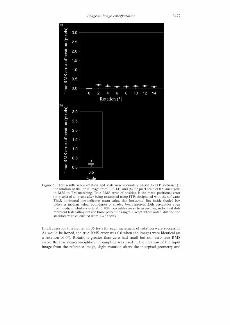
Image-to-image coregistration 3477
Figure 5. Test results when rotation and scale were accurately passed to ITP software: (a)for rotation of the input image from 0 to 14°; and (b) for pixel scale of 0.5, analogousto MSS to TM matching. True RMS error of position is the mean positional error(in pixels) of all pixels after being resampled using ITPs designated with the software.Thick horizontal line indicates mean value; thin horizontal line inside shaded boxindicates median value; boundaries of shaded box represent 25th percentiles awayfrom median; whiskers extend to 40th percentiles away from median; individual dotsrepresent tests falling outside those percentile ranges. Except where noted, distributionstatistics were calculated from n=35 tests.
In all cases for this figure, all 35 tests for each increment of rotation were successful.As would be hoped, the true RMS error was 0.0 when the images were identical (ata rotation of 0°). Rotations greater than zero had small but non-zero true RMSerror. Because nearest-neighbour resampling was used in the creation of the inputimage from the reference image, slight rotation alters the interpixel geometry and
R. E. Kennedy and W. B. Cohen3478
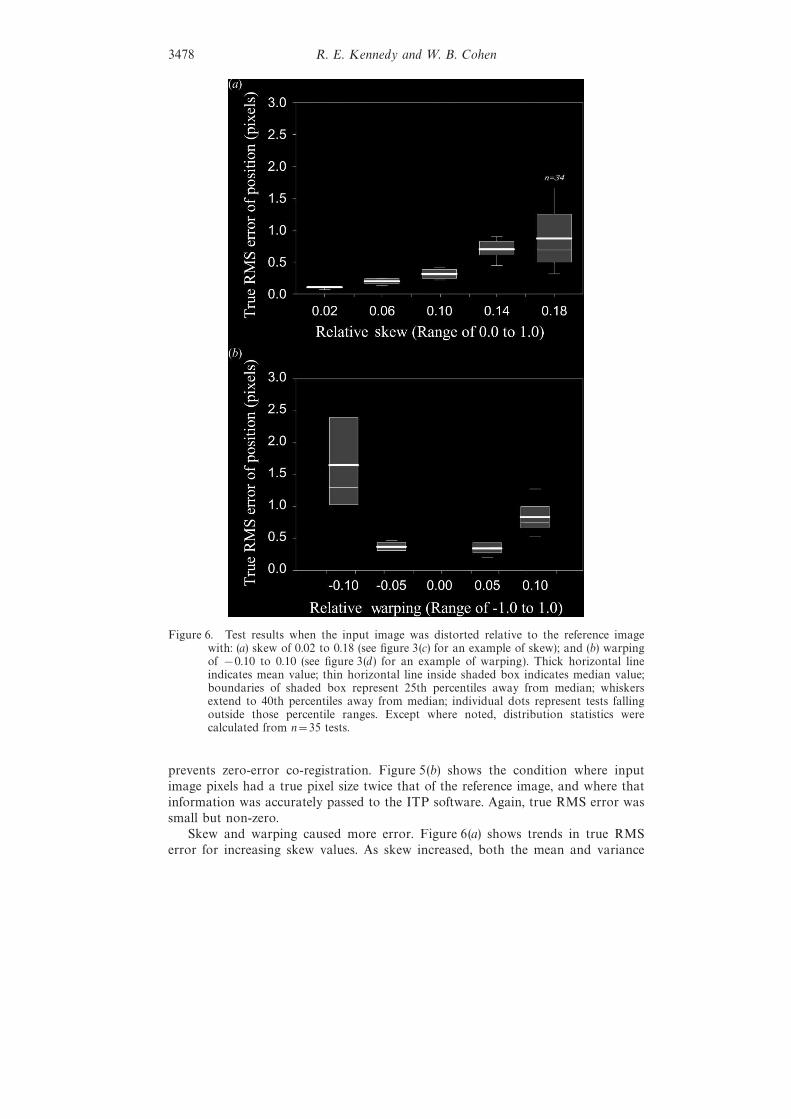
Figure 6. Test results when the input image was distorted relative to the reference imagewith: (a) skew of 0.02 to 0.18 (see figure 3(c) for an example of skew); and (b) warpingof −0.10 to 0.10 (see figure 3(d) for an example of warping). Thick horizontal lineindicates mean value; thin horizontal line inside shaded box indicates median value;boundaries of shaded box represent 25th percentiles away from median; whiskersextend to 40th percentiles away from median; individual dots represent tests fallingoutside those percentile ranges. Except where noted, distribution statistics werecalculated from n=35 tests.
prevents zero-error co-registration. Figure 5(b) shows the condition where inputimage pixels had a true pixel size twice that of the reference image, and where thatinformation was accurately passed to the ITP software. Again, true RMS error wassmall but non-zero.
Skew and warping caused more error. Figure 6(a) shows trends in true RMSerror for increasing skew values. As skew increased, both the mean and variance

Image-to-image coregistration 3479
about the mean increased. For skew values of 0.02 to 0.10, the mean and mediantrue RMS error values were below one-half pixel. An image with a skew of 0.10 willhave one side with length 10% narrower and the other side 10% wider than thecentre of the image, as illustrated in figure 3(c). In relation to skew, warping causedsimilar but amplified effects (figure 6(b)). At a warping of positive or negative 0.05,true RMS error was moderately low (means and medians less than 0.4 pixels). Itwas moderately higher for a warping value of positive 0.10, but much higher (greaterthan 1.0 pixel ) for a warping value of negative 0.10. Figure 3(d) provides a samplewarped image with a warping value of 0.10. An image with negative warping wouldhave convex rather than concave edges. Recall that for both skew and warping tests,only the input image is distorted; the reference image geometry remains as infigure 3(a).
3.2. Inaccurate input informationThe next set of tests involved situations where the user supplied the software
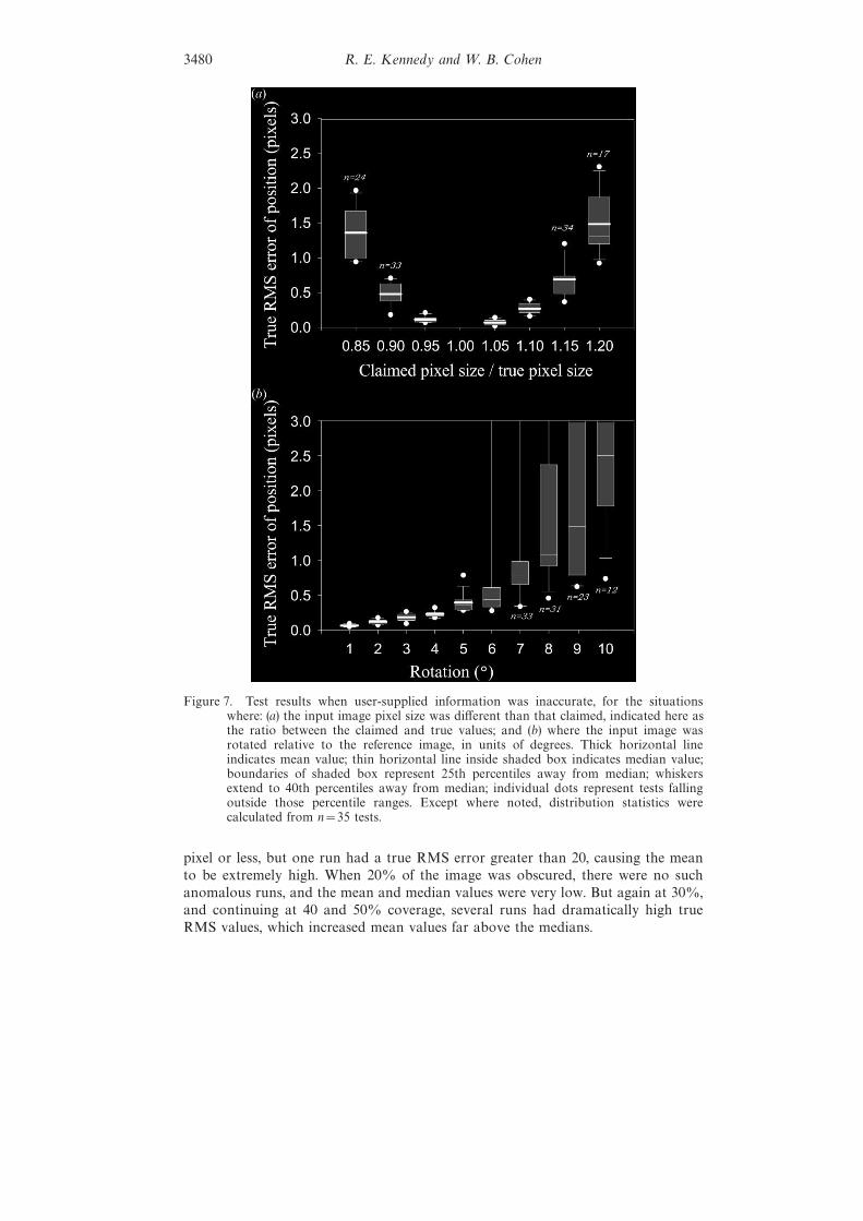
with inaccurate information about the images. Figure 7(a) shows how true RMSerror changed when true pixel size was inaccurate. When the true pixel size parameterof the input image was claimed to be within 5% of the actual value (true pixel sizedistortion of 0.95 to 1.05), the error was relatively small ( less than 0.2 pixels). Butwhen the distortion was 10%, true RMS error was near or over 0.5 pixels. By thetime distortion was 15%, error was large (near 1.5 pixels) and several tests failed(note that successful test counts indicated in the figure are much lower than thepossible 35), indicating that there were too few tie-points to adequately calculategeometric transformation matrices.
Undocumented rotation also caused error. In this situation, the input image wasrotated relative to the reference image, but the software was not informed of thatrotation. When the input image was rotated 5° relative to the reference image, themean and median true RMS error were under 0.5 pixels (figure 7(b)). When rotationreached 6°, however, variability in true RMS was much higher, and the mean wasmuch larger than the median. Three runs at a rotation of 6° had extremely high trueRMS values (>5 pixels). This is indicative of the breakdown of the software at higherrotations: by 10° of rotation, even the median true RMS value was near 2.5 pixels,and fewer than half of the runs (12 of 35) provided enough valid points to calculatea transformation matrix (figure 7(b)). For reference, figure 3(b) shows an example ofan image with a rotation of 6°.
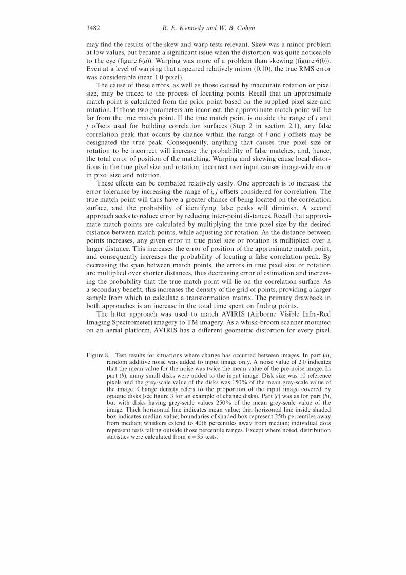
3.3. Change between imagesThe final tests were designed to emulate the situation where parts of the scene
change between images. Additive noise did little to reduce the effectiveness of theroutine (figure 8(a)), although a relative noise level of 2.0 confused the softwareenough to eliminate some tests from validity (only 28 of 35 runs successful ). Simulatedlandscape change also had little effect (figure 8(b)). Even when 50% of the inputimage was covered with opaque disks masking underlying patten (i.e. change densityof 0.5; see figure 3(e) for an example of change density of 0.5), true RMS error wasless than 0.2 pixels. The situation was less predictable when the opaque disks weremuch brighter than the background scene, as might be the case with clouds(figure 8(c)). True RMS error was much less predictable, and was generally higher,than for the simulated landscape changes. When 10% of the image was obscuredwith these brighter disks, all runs except one had true RMS error of a third of a
R. E. Kennedy and W. B. Cohen3480
Figure 7. Test results when user-supplied information was inaccurate, for the situationswhere: (a) the input image pixel size was different than that claimed, indicated here asthe ratio between the claimed and true values; and (b) where the input image wasrotated relative to the reference image, in units of degrees. Thick horizontal lineindicates mean value; thin horizontal line inside shaded box indicates median value;boundaries of shaded box represent 25th percentiles away from median; whiskersextend to 40th percentiles away from median; individual dots represent tests fallingoutside those percentile ranges. Except where noted, distribution statistics werecalculated from n=35 tests.
pixel or less, but one run had a true RMS error greater than 20, causing the meanto be extremely high. When 20% of the image was obscured, there were no suchanomalous runs, and the mean and median values were very low. But again at 30%,and continuing at 40 and 50% coverage, several runs had dramatically high trueRMS values, which increased mean values far above the medians.
Image-to-image coregistration 3481
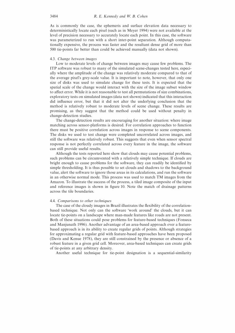
3.4. T ime per pointFigure 9 shows a histogram of the number of runs by the average number of
seconds per tie point in that run. This figure incorporates all runs referenced in thispaper. Recall that each run represents the average of up to 60 image tie points.Median time per point was 7.8 seconds. Because of the highly skewed distribution,the mean was much higher than the median (approximately 27 seconds per point).All runs were conducted on a Sun Ultra-1 workstation (1996 technology).
4. Discussion4.1. Overview
Correlation-based identification of image tie points has been criticized for beingtoo computationally expensive (Barnea and Silverman 1972, Brown 1992), and forbeing unable to handle certain types of image distortion (Pratt 1974) and cross-platform matching (Fonseca and Manjunath 1996). While these drawbacks certainlylimit its usefulness in some cases, correlation-based matching may be very helpfulfor many users. Our goal has been to introduce a software package that usescorrelation-based matching, and, more importantly, to test its constraints.
The tests provided herein were designed to be illustrative, not exhaustive.Nevertheless, we feel that the confounding factors we tested are an important subsetof those that might influence the ITP software. Two unaddressed factors in particularshould be considered before using the ITP software. First, to capture spatial pattern,the size of subset windows used to build the correlation indices (section 2.1) shouldbe much larger than the dominant spatial patterns of the images being matched. Astheir sizes converge, precision will drop. Second, the method of locating maximumspatial correlation requires that dark and light features in one image be correspond-ingly dark and light in the other. This will not necessarily be the case for imagesacquired on different platforms, as noted in many reviews of the subject (Rignotet al. 1991, Fonseca and Manjunath 1996). In summary, the utility of the methodwill ultimately depend upon the unique combination of scene spatial features, sensordetection characteristics, and the parameters used to run the ITP software.
4.2. Known and unknown distortionsThe tests reported here show that the ITP software can be useful under a wide
variety of conditions, although it does have limits. When the images were exactly asthe software expected i.e. when the user provided precisely accurate informationabout the images, the software was accurate and precise (figure 5(a)). The slightpixel-based error due to nearest neighbour resampling is an error source that waspresent in all of the tests, and was essentially impossible to separate on a test-by-test basis. Despite this error, the total error of position was minimal for both rotationand true pixel size differences, so long as those differences were accurately known(figure 5). This is likely the case for many users of satellite imagery: the images areminimally-distorted, any rotations are systematic and documented, and true pixelsize is relatively consistent and well-known.
Even when rotation and true pixel size were slightly inaccurate, error was stillrelatively small (figure 7). This suggests that the user need only provide roughestimates of these two quantities. Following the strategy of capitalizing on humanstrengths in pattern recognition, the user can quickly locate two approximate matchpoints and use simple trigonometry to gain these rough estimates.
Users of low-altitude aerial photography or of aerial scanners (such as AVIRIS)
R. E. Kennedy and W. B. Cohen3482
may find the results of the skew and warp tests relevant. Skew was a minor problemat low values, but became a significant issue when the distortion was quite noticeableto the eye (figure 6(a)). Warping was more of a problem than skewing (figure 6(b)).Even at a level of warping that appeared relatively minor (0.10), the true RMS errorwas considerable (near 1.0 pixel ).
The cause of these errors, as well as those caused by inaccurate rotation or pixelsize, may be traced to the process of locating points. Recall that an approximatematch point is calculated from the prior point based on the supplied pixel size androtation. If those two parameters are incorrect, the approximate match point will befar from the true match point. If the true match point is outside the range of i andj offsets used for building correlation surfaces (Step 2 in section 2.1), any falsecorrelation peak that occurs by chance within the range of i and j offsets may bedesignated the true peak. Consequently, anything that causes true pixel size orrotation to be incorrect will increase the probability of false matches, and, hence,the total error of position of the matching. Warping and skewing cause local distor-tions in the true pixel size and rotation; incorrect user input causes image-wide errorin pixel size and rotation.
These effects can be combated relatively easily. One approach is to increase theerror tolerance by increasing the range of i, j offsets considered for correlation. Thetrue match point will thus have a greater chance of being located on the correlationsurface, and the probability of identifying false peaks will diminish. A secondapproach seeks to reduce error by reducing inter-point distances. Recall that approxi-mate match points are calculated by multiplying the true pixel size by the desireddistance between match points, while adjusting for rotation. As the distance betweenpoints increases, any given error in true pixel size or rotation is multiplied over alarger distance. This increases the error of position of the approximate match point,and consequently increases the probability of locating a false correlation peak. Bydecreasing the span between match points, the errors in true pixel size or rotationare multiplied over shorter distances, thus decreasing error of estimation and increas-ing the probability that the true match point will lie on the correlation surface. Asa secondary benefit, this increases the density of the grid of points, providing a largersample from which to calculate a transformation matrix. The primary drawback inboth approaches is an increase in the total time spent on finding points.
The latter approach was used to match AVIRIS (Airborne Visible Infra-RedImaging Spectrometer) imagery to TM imagery. As a whisk-broom scanner mountedon an aerial platform, AVIRIS has a different geometric distortion for every pixel.
Figure 8. Test results for situations where change has occurred between images. In part (a),random additive noise was added to input image only. A noise value of 2.0 indicatesthat the mean value for the noise was twice the mean value of the pre-noise image. Inpart (b), many small disks were added to the input image. Disk size was 10 referencepixels and the grey-scale value of the disks was 150% of the mean grey-scale value ofthe image. Change density refers to the proportion of the input image covered byopaque disks (see figure 3 for an example of change disks). Part (c) was as for part (b),but with disks having grey-scale values 250% of the mean grey-scale value of theimage. Thick horizontal line indicates mean value; thin horizontal line inside shadedbox indicates median value; boundaries of shaded box represent 25th percentiles awayfrom median; whiskers extend to 40th percentiles away from median; individual dotsrepresent tests falling outside those percentile ranges. Except where noted, distributionstatistics were calculated from n=35 tests.

Image-to-image coregistration 3483
R. E. Kennedy and W. B. Cohen3484
As is commonly the case, the ephemeris and surface elevation data necessary todeterministically locate each pixel (such as in Meyer 1994) were not available at thelevel of precision necessary to accurately locate each point. In this case, the softwarewas parameterized to run with a short inter-point separation. Although computa-tionally expensive, the process was faster and the resultant dense grid of more than500 tie-points far better than could be achieved manually (data not shown).
4.3. Change between imagesLow to moderate levels of change between images may cause few problems. The
ITP software was robust to many of the simulated scene-changes tested here, especi-ally where the amplitude of the change was relatively moderate compared to that ofthe average pixel’s grey-scale value. It is important to note, however, that only onesize of disks was used to simulate change for these tests. It is expected that thespatial scale of the change would interact with the size of the image subset windowto affect error. While it is not reasonable to test all permutations of size combinations,exploratory tests on simulated images (data not shown) indicated that this interactiondid influence error, but that it did not alter the underlying conclusion that themethod is relatively robust to moderate levels of scene change. These results arepromising, as they suggest that the method could be used without penalty inchange-detection studies.
The change-detection results are encouraging for another situation: where imagematching across sensor-platforms is desired. For correlation approaches to functionthere must be positive correlation across images in response to scene components.The disks we used to test change were completed uncorrelated across images, andstill the software was relatively robust. This suggests that even when sensor spectralresponse is not perfectly correlated across every feature in the image, the softwarecan still provide useful results.
Although the tests reported here show that clouds may cause potential problems,such problems can be circumvented with a relatively simple technique. If clouds arebright enough to cause problems for the software, they can readily be identified bysimple thresholding. It is thus possible to set clouds and shadows to the backgroundvalue, alert the software to ignore those areas in its calculations, and run the softwarein an otherwise normal mode. This process was used to match TM images from theAmazon. To illustrate the success of the process, a tiled image composite of the inputand reference images is shown in figure 10. Note the match of drainage patternsacross the tile boundaries.
4.4. Comparisons to other techniquesThe case of the cloudy images in Brazil illustrates the flexibility of the correlation-
based technique. Not only can the software ‘work around’ the clouds, but it canlocate tie-points on a landscape where man-made features like roads are not present.Both of these situations could pose problems for feature-based techniques (Fonsecaand Manjunath 1996). Another advantage of an area-based approach over a feature-based approach is in its ability to create regular grids of points. Although strategiesfor approximating a regular grid with feature-based approaches have been proposed(Davis and Kenue 1978), they are still constrained by the presence or absence of arobust feature in a given grid cell. Moreover, area-based techniques can create gridsof tie-points at any arbitrary density.
Another useful technique for tie-point designation is a sequential-similarity
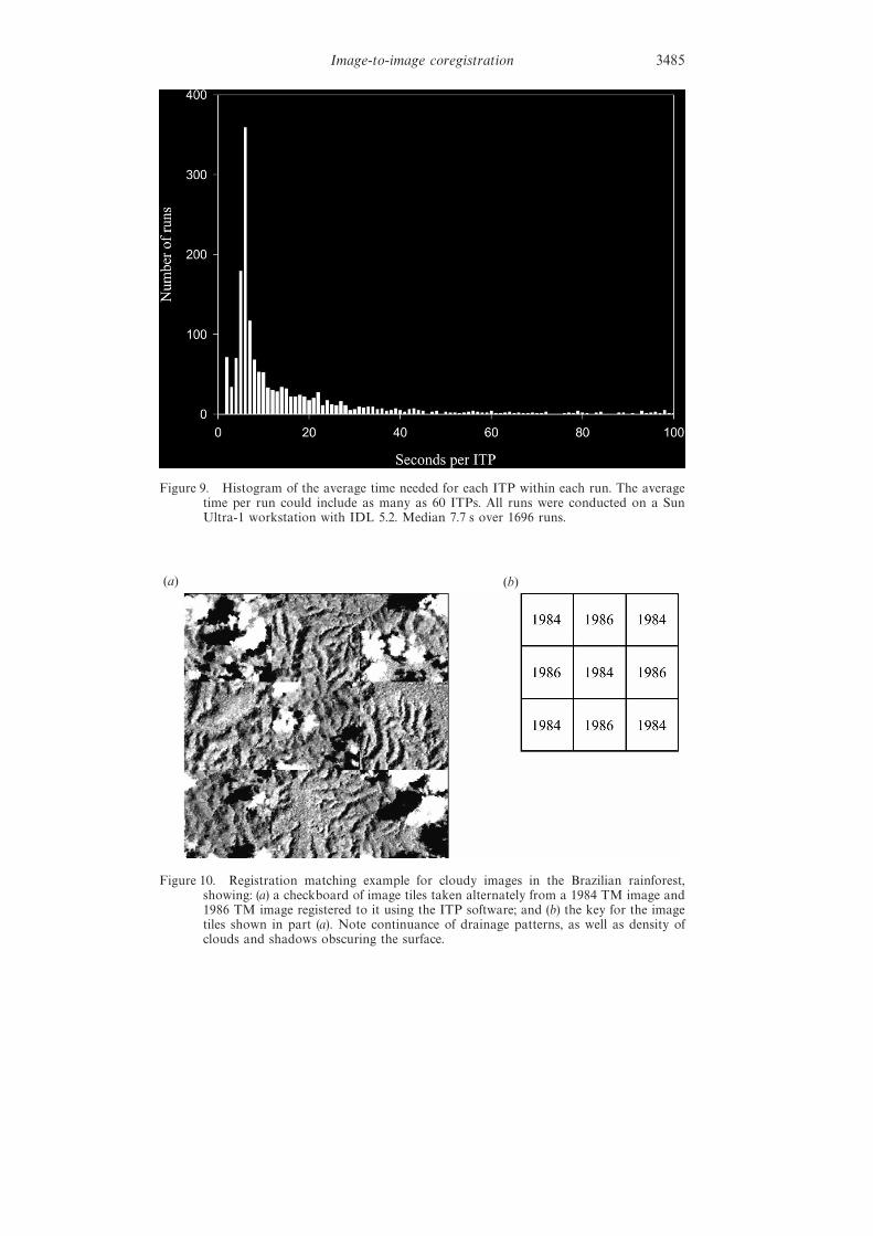
Image-to-image coregistration 3485
Figure 9. Histogram of the average time needed for each ITP within each run. The averagetime per run could include as many as 60 ITPs. All runs were conducted on a SunUltra-1 workstation with IDL 5.2. Median 7.7 s over 1696 runs.
(a) (b)
Figure 10. Registration matching example for cloudy images in the Brazilian rainforest,showing: (a) a checkboard of image tiles taken alternately from a 1984 TM image and1986 TM image registered to it using the ITP software; and (b) the key for the imagetiles shown in part (a). Note continuance of drainage patterns, as well as density ofclouds and shadows obscuring the surface.
R. E. Kennedy and W. B. Cohen3486
detection algorithm (SSDA; Barnea and Silverman 1972). Like a correlationapproach, an SSDA builds a similarity surface for a range of i, j offsets. For a givenoffset, absolute differences between pixel values are added sequentially in an increas-ing radius around a random point until a threshold is met. The similarity measureis the number of pixels added before the threshold is met; the matchpoint lies at themaximum. Although clearly faster than a correlation based approach, it may not beas robust across situations. Bernstein (1983) notes difficulty in designating a thresholdthat is generally applicable. Moreover, because the method includes only a sampleof the image subset pixels, it may be more susceptible to isolated anomalous features,such as regions of changed pixels. In the search for a general approach, then, theSSDA may not be as useful as a correlation-based approach.
In contrast to both feature-based approaches and the SSDA strategy, correlationtechniques allow for subpixel approximation of matchpoint position (Bernstein 1983).This is again computationally expensive, but may be useful where high precision isrequired.
4.5. Computational costsThe biggest criticism of correlation-based approaches is their high computational
expense. Yet with today’s computers, the computational cost of the correlation-basedapproaches may be small enough to be insignificant for many potential users.Approximately 75% of the runs reported here had a mean time per ITP under 20seconds, and 90% were under 1 minute. In practice, we have found that new TMimages can be accurately, repeatably matched and resampled in under 45 minutes,with user attention required for only a few minutes of that time.
4.6. Examples of applicationsWe have applied the software successfully in many situations and environments.
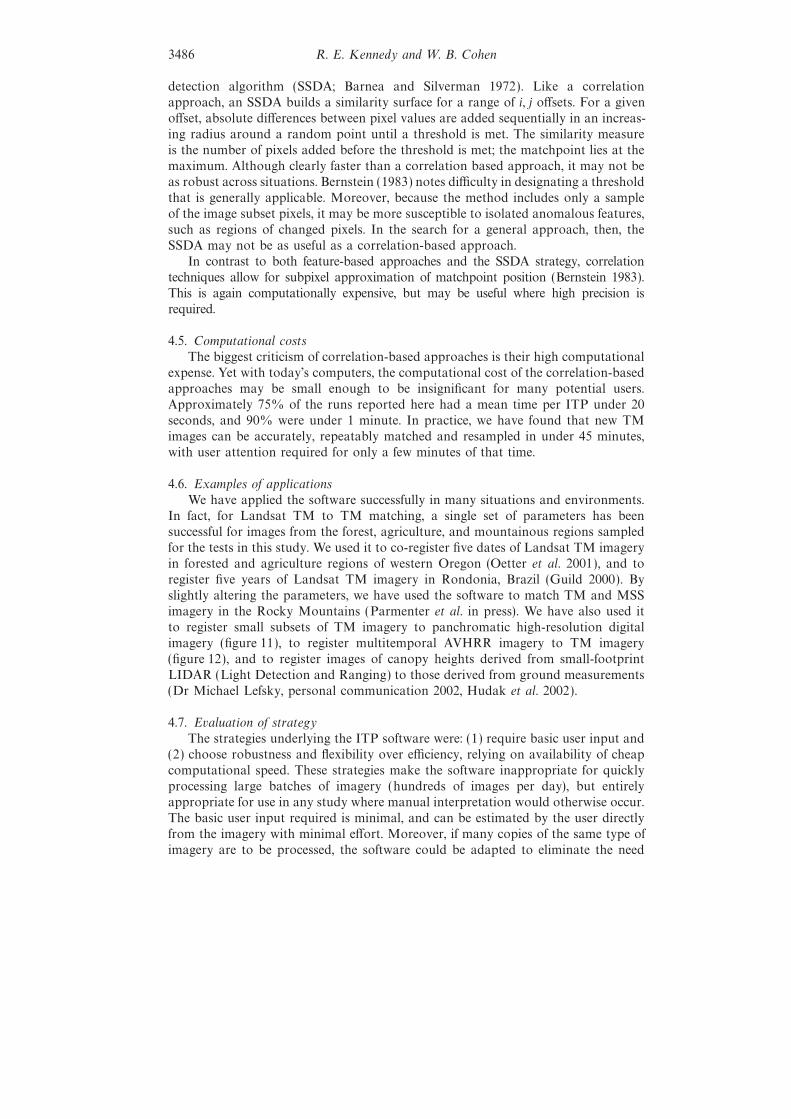
In fact, for Landsat TM to TM matching, a single set of parameters has beensuccessful for images from the forest, agriculture, and mountainous regions sampledfor the tests in this study. We used it to co-register five dates of Landsat TM imageryin forested and agriculture regions of western Oregon (Oetter et al. 2001), and toregister five years of Landsat TM imagery in Rondonia, Brazil (Guild 2000). Byslightly altering the parameters, we have used the software to match TM and MSSimagery in the Rocky Mountains (Parmenter et al. in press). We have also used itto register small subsets of TM imagery to panchromatic high-resolution digitalimagery (figure 11), to register multitemporal AVHRR imagery to TM imagery(figure 12), and to register images of canopy heights derived from small-footprintLIDAR (Light Detection and Ranging) to those derived from ground measurements(Dr Michael Lefsky, personal communication 2002, Hudak et al. 2002).
4.7. Evaluation of strategyThe strategies underlying the ITP software were: (1) require basic user input and
(2) choose robustness and flexibility over efficiency, relying on availability of cheapcomputational speed. These strategies make the software inappropriate for quicklyprocessing large batches of imagery (hundreds of images per day), but entirelyappropriate for use in any study where manual interpretation would otherwise occur.The basic user input required is minimal, and can be estimated by the user directlyfrom the imagery with minimal effort. Moreover, if many copies of the same type ofimagery are to be processed, the software could be adapted to eliminate the need
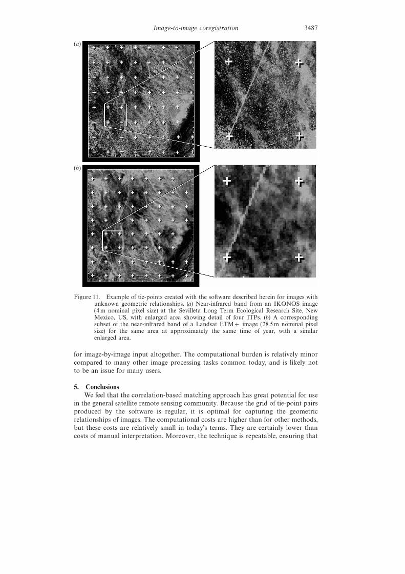
Image-to-image coregistration 3487
(a)
(b)
Figure 11. Example of tie-points created with the software described herein for images withunknown geometric relationships. (a) Near-infrared band from an IKONOS image(4 m nominal pixel size) at the Sevilleta Long Term Ecological Research Site, NewMexico, US, with enlarged area showing detail of four ITPs. (b) A correspondingsubset of the near-infrared band of a Landsat ETM+ image (28.5 m nominal pixelsize) for the same area at approximately the same time of year, with a similarenlarged area.
for image-by-image input altogether. The computational burden is relatively minorcompared to many other image processing tasks common today, and is likely notto be an issue for many users.
5. ConclusionsWe feel that the correlation-based matching approach has great potential for use
in the general satellite remote sensing community. Because the grid of tie-point pairsproduced by the software is regular, it is optimal for capturing the geometricrelationships of images. The computational costs are higher than for other methods,but these costs are relatively small in today’s terms. They are certainly lower thancosts of manual interpretation. Moreover, the technique is repeatable, ensuring that

R. E. Kennedy and W. B. Cohen3488
(a)
(b)
Figure 12. As figure 11, but for imagery acquired over western Oregon, US. (a) The greennessband from a tasselled-cap transformation of Landsat TM data (28.5 m nominal pixelsize) mosaicked from five scenes, with an enlargement to show detail around nineITPs. (b) An NDVI image composited from two weeks of AVHRR imagery (nominalpixel size 1 km; data courtesy Brad Reed, USGS EROS Data Center) around the sametime as the TM scene, with an enlargement showing detail for an area of nine ITPs.
image libraries built up over time have consistent geometric properties. It is relativelyrobust to simple distortions and inaccuracies, although special attention must bepaid to warping and to inaccuracies in pixel size estimation. Nevertheless, thecorrelation-based approach is flexible, and the software allows complete control overimage-matching parameters. By focusing on robustness over absolute efficiency, andby relying on simple user input, we feel that correlation-based software can be usefulto many users in the remote-sensing community.
AcknowledgmentsFunding for this project was provided from NASA through the Terrestrial
Ecology Program, the EPSCOR program, and the Land Cover Land Use Change
Image-to-image coregistration 3489
program. Additional support came from the NSF-funded LTER program at the H. J.Andrews Experimental Forest, and from the USDA Forest Service Pacific NorthwestStation’s Ecosystem Processes program. The authors would like to thank KarinFassnacht and Andrew Hudak for helpful comments on the manuscript, AndyHansen for collaboration on one of the funding projects, Greg Asner for imagesfrom Brazil, Brad Reed for AVHRR composite imagery, and Alisa Gallant, DouglasOetter, Tom Maiersperger, Keith Olsen, Michael Lefsky, Mercedes Berterreche, andAndrea Wright Parmenter for comments on the software package described herein.
ReferencesB, D. I., and S, H. F., 1972, A class of algorithms for fast digital image
registration. IEEE T ransactions on Geoscience and Remote Sensing, 21, 179–186.B, R., 1983, Image geometry and rectification. In Manual of Remote Sensing, edited
by R. Colwell (Falls Church, VA: American Society of Photogrammetry), pp. 873–922.B, L. G., 1992, A survey of image registration techniques. ACM Computing Surveys,
24, 325–376.D,W.A., andK, S.K., 1978, Automatic selection of control points for the registration
of digital images. Proceedings of the Fourth International Joint Conference on PatternRecognition, Kyoto, Japan (New York: IEEE), pp. 936–938.
F, L. M. G., and M, B. S., 1996, Registration techniques for multisensorremotely sensed imagery. Photogrammetric Engineering and Remote Sensing, 62,1049–1056.
G, A., S, G. C., and P, C. V., 1986, A region-based approach to digitalimage registration with subpixel accuracy. IEEE T ransactions on Geoscience andRemote Sensing, 24, 390–399.
G, L. S., 2000, Detection of deforestation and conversion and estimation of atmosphericemissions and elemental pool losses from biomass burning in Rondonia, Brazil. PhDthesis, Oregon State University, 120 pp.
H, A. T., L, M. A., C, W. B., and B, M., 2002, Integration oflidar and Landsat ETM+ data for estimating and mapping forest canopy height.Remote Sensing of Environment, 82, 397–416.
L, H.,M, B. S., andM, S. K., 1995, A contour-based approach to multisensorimage registration. IEEE T ransactions on Geoscience and Remote Sensing, 4, 320–334.
L, M., 1991, Hierarchical multipoint matching. Photogrammetric Engineering and RemoteSensing, 57, 1039–1047.
M, P., 1994, A parametric approach for the geocoding of airborne visible/infrared imagingspectrometer (AVIRIS) data in rugged terrain. Remote Sensing of Environment, 49,118–130.
O, D. R., C,W. B., B,M.,M, T. K., and K, R. E.,2001, Land cover mapping in an agricultural setting using multi-seasonal ThematicMapper data. Remote Sensing of Environment, 76, 139–155.
P, A. W., H, A., K, R., L, U., C, W., L, R.,M, B., A, R., and G, A., in press, Land use and land coverchange in the Greater Yellowstone Ecosystem: 1975–1995. Ecological Applications.
P, W. K., 1974, Correlation techniques of image registration. IEEE T ransactions onAerospace and Electronic Systems, 10, 353–358.
P, W. K., 1991, Digital Image Processing (New York: John Wiley and Sons, Inc.).R, E. J., K, R., C, J. C., and P, S. S., 1991, Automated multisensor
registration: requirements and techniques. Photogrammetric Engineering and RemoteSensing, 57, 1029–1038.
R, D., 1987, Multi-point matching using the least-squares technique for evaluationof three-dimensional models. Photogrammetric Engineering and Remote Sensing, 53,621–626.
S, T. A., D, M. J., W, J. C., and B, R. A., 1992,Application of image cross-correlation to the measurement of glacier velocity usingsatellite image data. Remote Sensing of Environment, 42, 177–186.

Image-to-image coregistration3490
S, R. A., 1997, Remote Sensing: Models and methods for image processing (SanDiego: Academic Press).
T, Y.-H., T, J.-J., T, K.-P., and L, S.-H., 1997, Image-to-image registration bymatching area features using fourier descriptors and neural networks. PhotogrammetricEngineering and Remote Sensing, 63, 975–983.