Automated Force Field Parameterization for Atomic Models

Based on Ab Initio Target Data

Li-Ping XU

Supervisor: Prof. Wiest

Prof. Wu

Introduction

• Force fields in molecular mechanics

• The ingredients of a force field

• Functional form

• Reference data

• Optimization method

General Automated Atomic Model Parameterization

• Overview of method

• Results and discussion

• Limitation and possible improvements

Outline

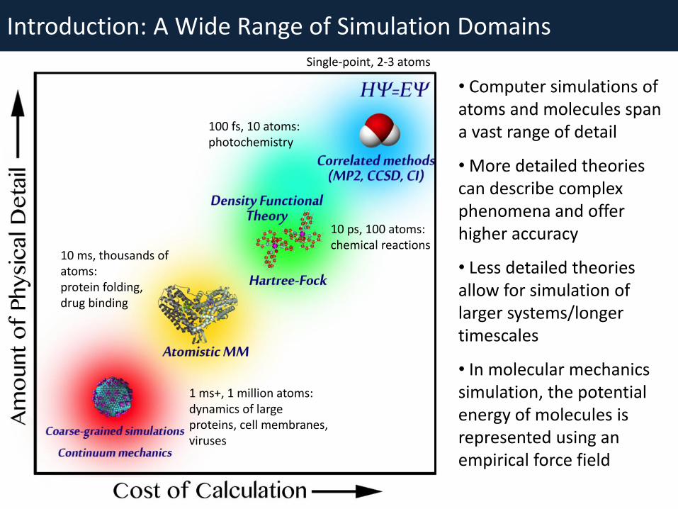
• Computer simulations of atoms and molecules span a vast range of detail

• More detailed theories can describe complex phenomena and offer higher accuracy

• Less detailed theories allow for simulation of larger systems/longer timescales

• In molecular mechanics simulation, the potential energy of molecules is represented using an empirical force field

10 ps, 100 atoms: chemical reactions

100 fs, 10 atoms: photochemistry

10 ms, thousands of atoms: protein folding, drug binding

Single-point, 2-3 atoms

1 ms+, 1 million atoms: dynamics of large proteins, cell membranes, viruses

Introduction: A Wide Range of Simulation Domains

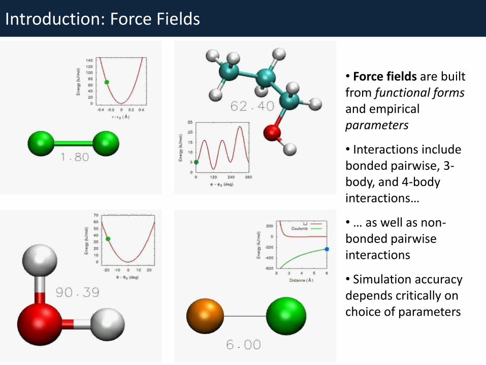
Introduction: Force Fields

• Force fields are built from functional forms and empirical parameters

• Interactions include bonded pairwise, 3-body, and 4-body interactions…

• … as well as non-bonded pairwise interactions

• Simulation accuracy depends critically on choice of parameters

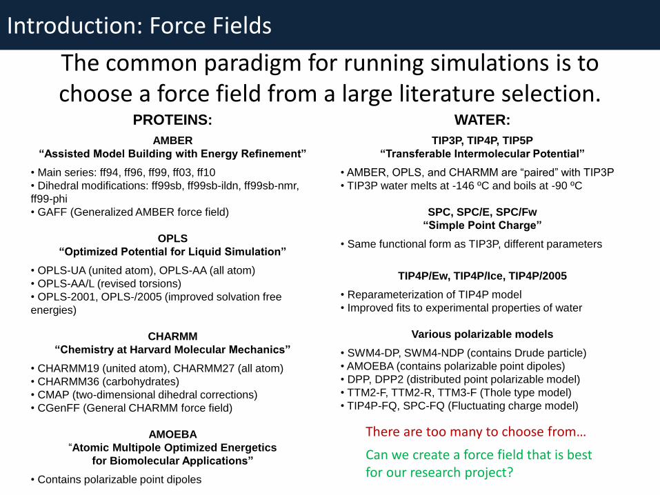
Introduction: Force Fields

The common paradigm for running simulations is to choose a force field from a large literature selection.

PROTEINS:

AMBER

“Assisted Model Building with Energy Refinement”

• Main series: ff94, ff96, ff99, ff03, ff10

• Dihedral modifications: ff99sb, ff99sb-ildn, ff99sb-nmr,

ff99-phi

• GAFF (Generalized AMBER force field)

OPLS

“Optimized Potential for Liquid Simulation”

• OPLS-UA (united atom), OPLS-AA (all atom)

• OPLS-AA/L (revised torsions)

• OPLS-2001, OPLS-/2005 (improved solvation free

energies)

CHARMM

“Chemistry at Harvard Molecular Mechanics”

• CHARMM19 (united atom), CHARMM27 (all atom)

• CHARMM36 (carbohydrates)

• CMAP (two-dimensional dihedral corrections)

• CGenFF (General CHARMM force field)

AMOEBA

“Atomic Multipole Optimized Energetics

for Biomolecular Applications”

• Contains polarizable point dipoles

WATER:

TIP3P, TIP4P, TIP5P

“Transferable Intermolecular Potential”

• AMBER, OPLS, and CHARMM are “paired” with TIP3P

• TIP3P water melts at -146 ºC and boils at -90 ºC

SPC, SPC/E, SPC/Fw

“Simple Point Charge”

• Same functional form as TIP3P, different parameters

TIP4P/Ew, TIP4P/Ice, TIP4P/2005

• Reparameterization of TIP4P model

• Improved fits to experimental properties of water

Various polarizable models

• SWM4-DP, SWM4-NDP (contains Drude particle)

• AMOEBA (contains polarizable point dipoles)

• DPP, DPP2 (distributed point polarizable model)

• TTM2-F, TTM2-R, TTM3-F (Thole type model)

• TIP4P-FQ, SPC-FQ (Fluctuating charge model)

There are too many to choose from…

Can we create a force field that is best for our research project?

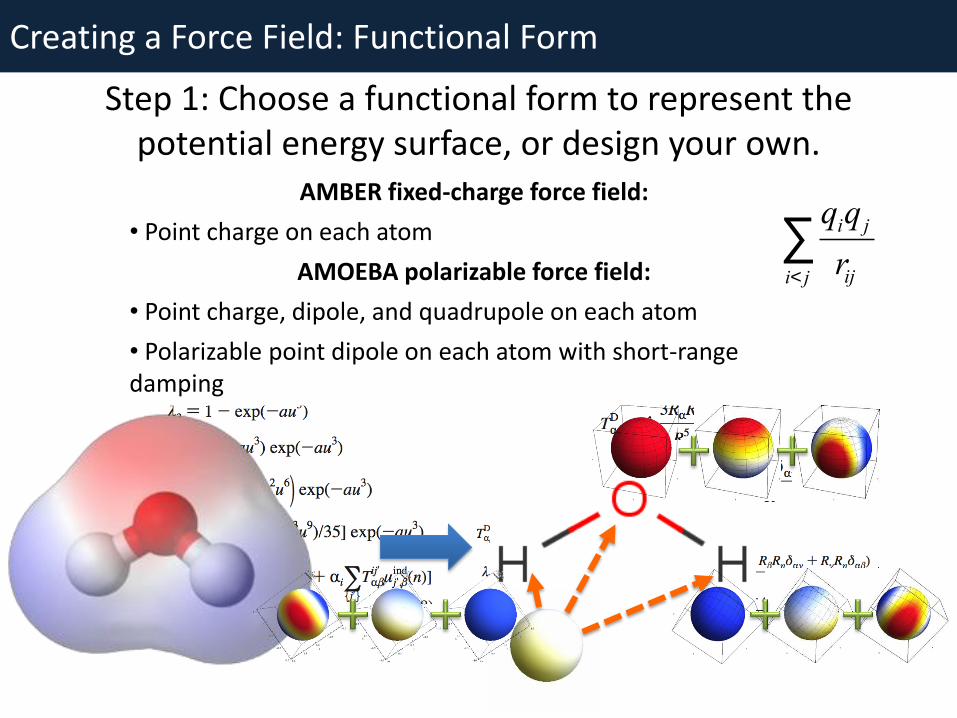
Creating a Force Field: Functional Form

Step 1: Choose a functional form to represent the potential energy surface, or design your own.

AMBER fixed-charge force field:

• Point charge on each atom

AMOEBA polarizable force field:

• Point charge, dipole, and quadrupole on each atom

• Polarizable point dipole on each atom with short-range damping

qiq j

riji< j

å

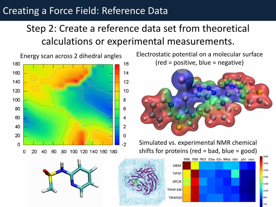
Creating a Force Field: Reference Data

Step 2: Create a reference data set from theoretical calculations or experimental measurements.

Energy scan across 2 dihedral angles Electrostatic potential on a molecular surface (red = positive, blue = negative)

Simulated vs. experimental NMR chemical shifts for proteins (red = bad, blue = good)

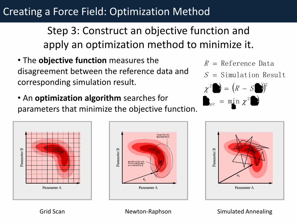
Creating a Force Field: Optimization Method

• The objective function measures the disagreement between the reference data and corresponding simulation result.

• An optimization algorithm searches for parameters that minimize the objective function.

kk

kk

k

2

22

min

Result Simulation

Data Reference

opt

SR

S

R

Step 3: Construct an objective function and apply an optimization method to minimize it.

Grid Scan Newton-Raphson Simulated Annealing

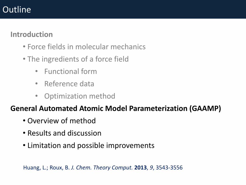
Introduction

• Force fields in molecular mechanics

• The ingredients of a force field

• Functional form

• Reference data

• Optimization method

General Automated Atomic Model Parameterization (GAAMP)

• Overview of method

• Results and discussion

• Limitation and possible improvements

Outline

Huang, L.; Roux, B. J. Chem. Theory Comput. 2013, 9, 3543-3556

Introducing GAAMP

There are some tools for parameterization of novel molecules: • Antechamber: automatically parameterize small

compounds in accord with general Amber force field (GAFF) • CGenFF: provide CHARMM-consistent force field

parameters for small compounds and drug-like molecules.

However, partial charges and dihedral parameters have limited transferabilities. The accuracy is still a problem.

Introducing GAAMP

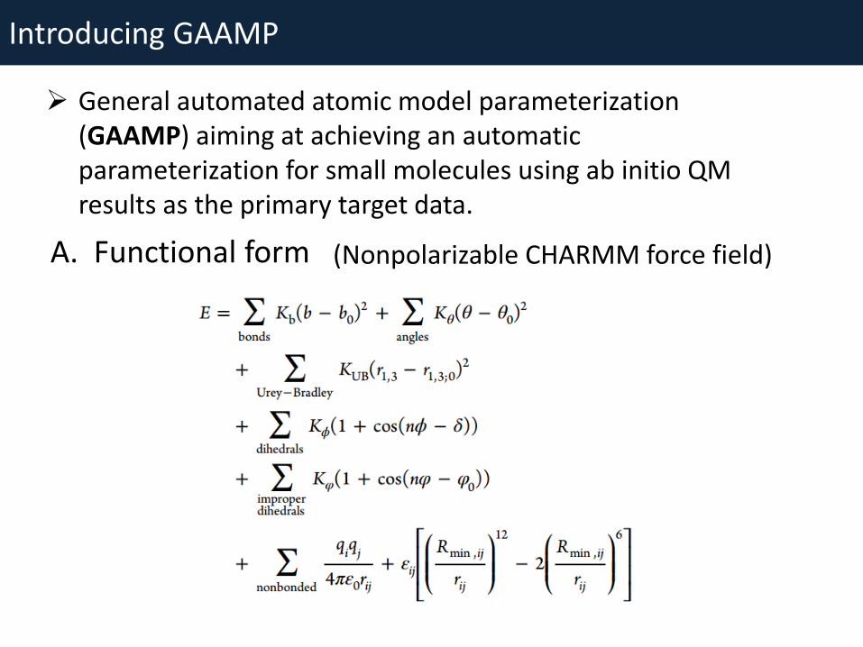
General automated atomic model parameterization (GAAMP) aiming at achieving an automatic parameterization for small molecules using ab initio QM results as the primary target data.

(Nonpolarizable CHARMM force field) A. Functional form

Introducing GAAMP

1. Bond length and angle parameters: from GAFF, CGenFF geometry or QM calculation 2. Charge fitting: combination of ESP fitting and compound-water interaction fitting

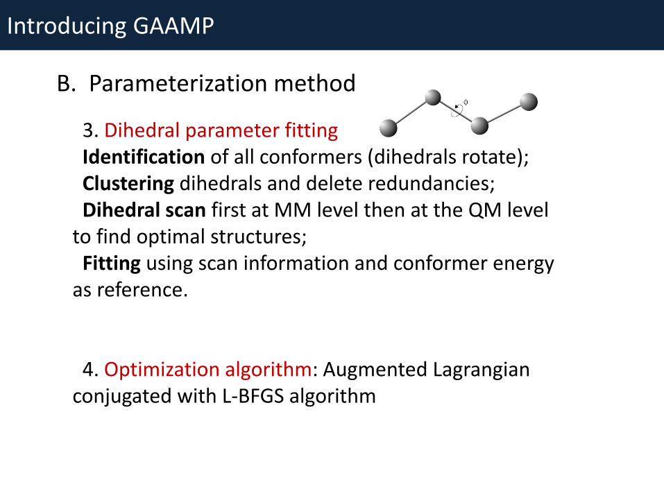
B. Parameterization method

Introducing GAAMP

3. Dihedral parameter fitting Identification of all conformers (dihedrals rotate); Clustering dihedrals and delete redundancies; Dihedral scan first at MM level then at the QM level to find optimal structures; Fitting using scan information and conformer energy as reference. 4. Optimization algorithm: Augmented Lagrangian conjugated with L-BFGS algorithm

B. Parameterization method

GAAMP: Result and Discussion

Results 1. Dihedral parameters

φ1 = 1-2-3-4 φ2 = 2-3-4-6 φ3 = 3-4-6-7

GAFF/AM1-BCC works reasonably for this molecule; GAAMP perfectly matches QM results of the dihedral energy profiles; QM conformer energies also can be reproduced well.

GAAMP: Result and Discussion

Results 1. Dihedral parameters

GAFF/AM1-BCC does not perform well For φ4 and φ6; GAAMP can reproduce QM energy Profiles reasonably well for all dihedrals.

“Gleevec”

GAAMP: Result and Discussion

Results 2. Solvation free energies of 217 compounds

98 compounds without hydrogen-bond donor/acceptor

AUE = 0.74 kcal/mol AUE = 0.58 kcal/mol

GAFF/AM1-BCC GAAMP/RESP

AUE: average unassigned error, the lower, the better.

GAAMP: Result and Discussion

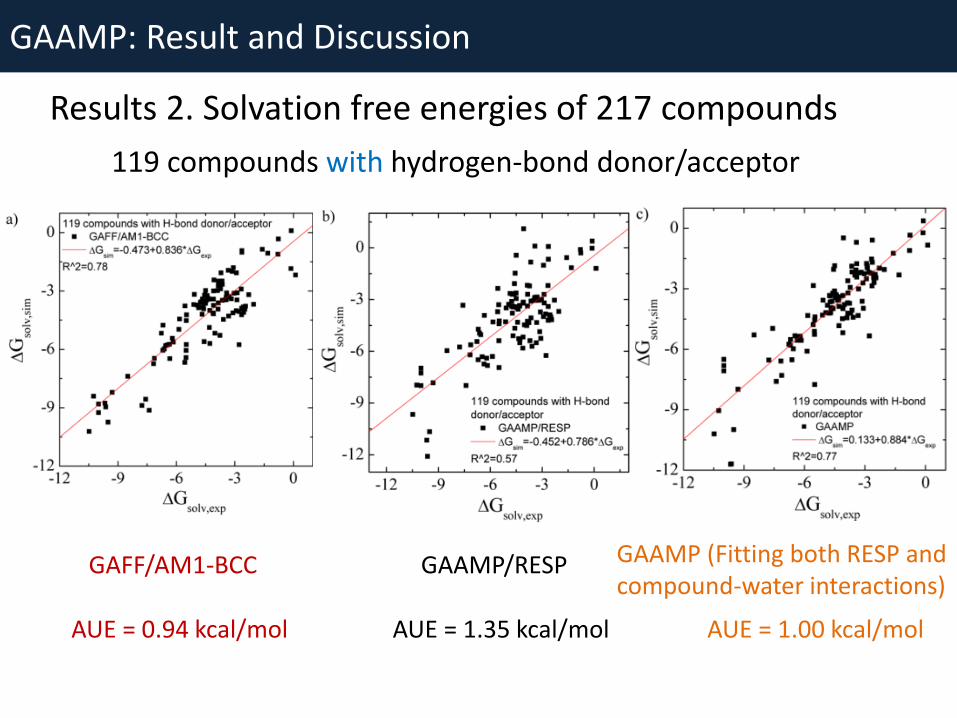
Results 2. Solvation free energies of 217 compounds

AUE = 0.94 kcal/mol AUE = 1.00 kcal/mol

GAFF/AM1-BCC GAAMP/RESP GAAMP (Fitting both RESP and compound-water interactions)

AUE = 1.35 kcal/mol

119 compounds with hydrogen-bond donor/acceptor

GAAMP: Result and Discussion

Results 2. Solvation free energies of 217 compounds

AUE = 0.85 kcal/mol AUE = 0.81 kcal/mol

GAFF/AM1-BCC

217 compounds including both polar and nonpolar molecules

GAAMP (Fitting both RESP and compound-water interactions)

GAAMP: Result and Discussion

Results 3. GAAMP vs CHARMM27 in protein simulation

CHARMM27 GAAMP

Four independent 100 ns simulation from crystal structure

The protein is stable both in CHARMM27 and GAAMP with conformational fluctuations.

The parameters of amino acids generated by GAAMP are consistent with existing CHARMM27.

GAAMP: Result and Discussion

Results 3. GAAMP vs CHARMM27 in protein simulation

CHARMM27 GAAMP

Four independent 100 ns simulation from crystal structure

GAAMP: Limitations and Possible Improvements

GAAMP targets ab initio calculations, which could be expensive.

Cut large molecule into smaller fragments, parameterize them separately, then join them together.

Geometry optimization is performed in a vacuum. QM geometry optimization with a continuum solvent method. For molecules inherently not supported by GAFF or CGenFF,

hard to get initial parameters, hard to parameterize. Manually or use other force field development method, such

as Q2MM, to prepare a reasonable initial FF

Thank You for Your Listening!