automated lod-2 model reconstruction from very-high

To appear in ISPRS Journal of photogrammetry and Remote Sensing (2021)

Automated LoD-2 Model Reconstruction from Very-High-

Resolution Satellite-derived Digital Surface Model and

Orthophoto

Shengxi Gui a,b, Rongjun Qin a,b,c,d,*

a Geospatial Data Analytics Lab, The Ohio State University, Columbus, USA;

b Department of Civil, Environmental and Geodetic Engineering, The Ohio State University, Columbus,

USA;

c Department of Electrical and Computer Engineering, The Ohio State University, Columbus, USA;

d Translational Data Analytics Institute, The Ohio State University, Columbus, USA;

*Corresponding author: [email protected], 2036 Neil Avenue, Columbus Ohio 43210, USA.

Abstract:

Digital surface models (DSM) generated from multi-stereo satellite images are getting higher in quality

owing to the improved data resolution and photogrammetric reconstruction algorithms. Very-high-

resolution (VHR, with sub-meter level resolution) satellite images effectively act as a unique data source

for 3D building modeling, because it provides a much wider data coverage with lower cost than the

traditionally used LiDAR and airborne photogrammetry data. Although 3D building modeling from point

clouds has been intensively investigated, most of the methods are still ad-hoc to specific types of buildings

and require high-quality and high-resolution data sources as input. Therefore, when applied to satellite-

based point cloud or DSMs, these developed approaches are not readily applicable and more adaptive and

robust methods are needed. As a result, most of the existing work on building modeling from satellite DSM

achieves LoD-1 generation. In this paper, we propose a model-driven method that reconstructs LoD-2

building models following a "decomposition-optimization-fitting” paradigm. The proposed method starts

building detection results through a deep learning-based detector and vectorizes individual segments into

polygons using a “three-step” polygon extraction method, followed by a novel grid-based decomposition

method that decomposes the complex and irregularly shaped building polygons to tightly combined

elementary building rectangles ready to fit elementary building models. We have optionally introduced

OpenStreetMap (OSM) and Graph-Cut (GC) labeling to further refine the orientation of 2D building

rectangle. The 3D modeling step takes building-specific parameters such as hip lines, as well as non-rigid

and regularized transformations to optimize the flexibility for using a minimal set of elementary models.

Finally, roof type of building models s refined and adjacent building models in one building segment are

merged into the complex polygonal model. Our proposed method has addressed a few technical caveats

over existing methods, resulting in practically high-quality results, based on our evaluation and

comparative study on a diverse set of experimental datasets of cities with different urban patterns. (codes

/binaries may be available under this GitHub page: https://github.com/GDAOSU/LOD2BuildingModel)

Keywords:

LoD-2 Building Modeling, data-driven, decomposition and merging, multi-stereo satellite images

mailto:[email protected]


1. Introduction

Remotely sensed satellite imagery effectively acts as one of the preferred ways to reconstruct wide-

area and low-cost 3D building models used in urban and regional scale studies (Brown et al., 2018;

Facciolo et al., 2017; Leotta et al., 2019). However, because satellite imagery has a relatively lower spatial

resolution than aerial imagery and LiDAR, 3D building models base on satellite data faces challenges in

detecting buildings, extracting building boundaries, and reconstructing an accurate building 3D model,

especially in regions with small and dense buildings (Sirmacek & Unsalan, 2011). Level-of-Detail (LoD)

building models defined through the city geography markup language (CityGML), present 3D building

models in several levels 0 to 4 (Gröger et al., 2008). An improved LoD standard CityGML 2.0 speciate

LoD-0 to LoD-3 as four sub-definitions from LoD x.0 to LoD x.3 bases on the exterior geometry of

buildings (Gröger et al., 2012; Biljecki et al., 2016). With relatively fine digital surface models derived

from satellite photogrammetry, using satellite-based DSM and building polygon to generate Level-of-

Detail 1 (LoD-1) 3D building models with a flat roof is now becoming a standard practice. However, 3D

building models reconstruction with prototypical roof structures (LoD-2), remains a challenging problem,

especially from low-cost data sources such as satellite images (Kadhim & Mourshed, 2018; Bittner &

Korner, 2018). Despite the increasingly higher resolution of satellite images (as high as 0.3-0.5 GSD) on

par with past aerial images, the generated 3D information from the satellite images, due to 1) image quality

(being high altitude collection distorted by the atmosphere), 2) relatively low resolution in comparison to

aerial data, and 3) cross-track collections (Qin, 2019) with temporal variations, often posses high

uncertainties leading to challenges in LoD-2 modeling. Although 3D building modeling from point clouds

has been intensively studied, most of the methods are still ad-hoc to specific types of buildings and assume

these input point clouds to be highly accurate and dense (i.e. those captured with LiDAR). However, when

presented with low-resolution point clouds with relatively high uncertainties as produced by satellite

images, these methods no longer produce reasonable results, especially for areas with dense buildings, as

traditional bottom-up approaches are not able to identify and separate between individual buildings given

the low resolution and blurry boundaries both in height (from digital surface models (DSM) or point

clouds) and in color (or spectrum), therefore it requires approaches to be sufficiently robust to identify,

regularize and extract individual buildings, often following a top-down approach (i.e. model-driven). To

extract individual and well-delineated boundaries of the building, one often needs to decompose

“overestimated” building footprint candidates, using regularity, spectral or height cues (Brédif et al., 2013;

Partovi et al., 2019), and adapt models that are well-suited to the extracted/decomposed footprints.

However, among the limited studies focusing on LoD-2 reconstruction based on satellite-derived DSMs

(Alidoost et al., 2019; Partovi et al., 2019; Woo & Park, 2011), caveats exist in the decomposition

procedure, which often does not fully explore the use spectrum, DSM and contextual information, resulting

in unsatisfactory results, especially in areas where buildings are dense: on the one hand the individual

buildings are often incorrectly extracted/oriented, on the other hand, buildings in clusters are not consistent.

In this paper, we revisit this process and fill a number of gaps by developing a three-step approach

that specifically aims to improve the extraction of building polygon and fitting models in such challenging

cases, which formed our proposed LoD-2.0 model reconstruction pipeline for satellite-derived DSM and

Orthophotos: our proposed method starts with building mask detection by using a weighted U-Net and

RCNN (region-based Convolutional Neural Networks), followed by the proposed three-step approach


through “extraction-decomposition- refinement” for regularized 2D building rectangle generation. In the

“extraction” step, we vectorize building masks as boundary lines, and then regularize lines orientation

through line segments from orthophoto. In the “decomposition” step, a grid-based building rectangle

generating method is developed by a grid pyramid to generate rectangles and subsequent separating and

merging steps to optimize polygons. In the “refinement” step, we post-refine the 2D model parameters

through propagating similarities of neighboring buildings (in terms of their orientation and type) through a

Graph-Cut (GC) algorithm, with optionally a second refinement step using OpenStreetMap road vector

data. The individual building rectangle and the corresponding DSMs are then fitted by taking models from

a pre-defined model library that minimizes the difference between the model and the DSM. In this process,

the motivation is to fully utilize the spectral and height information when performing the decomposition

process and take global assumptions on orientation and building type consistencies of the building clusters

to yield results that are superior to state-of-the-art methods. The proposed method is validated using a

diverse set of data, and although our approach follows and refines the existing modeling paradigm, we find

the proposed approach yields robust performance on various types of data and is able to reconstruct areas

with dense urban buildings. This therefore leads to our contributions in this paper: 1) we present a model-

driven workflow that performs LoD-2 model reconstruction that yields highly accurate results as compared

to state-of-the-art methods; 2) We demonstrate that the use of a combined semantic segmentation and

Region-based CNN (RCNN) leverages detection and completeness for object-level mask generation; 3) we

propose a novel three-stage (“extraction-decomposition-refinement”) approach to perform vectorization of

building masks that yields superior performance; 4) We validate that the use of multiple cues of

neighboring buildings, and optionally road vector maps, can generally improve the accuracy of the

resulting reconstruction.

The remainder of the paper is organized as follows: Section 2 introduces related works, and Section 3

describes our approach for 3D building modeling in detail, includes pre-processing, building detection and

segmentation, building footprint extraction, building polygon decomposition, building polygon orientation

refinement, 3D building model fitting, adjacent building model merging. Section 4 summarizes four study

areas in two cities and experiment results of qualitative and quantitative evaluation, and the comparison

with other current methods. Finally, Section 5 concludes this paper.

2. Related work

There are many approaches for the detection and reconstruction of 3D building models from airborne

photogrammetry and LiDAR data (Cheng et al., 2011; Wang, 2013), and relatively few on the satellite-

derived data (Arefi & Reinartz, 2013; Woo & Park, 2011) given that dense matching method yielding

relatively high-quality data was only getting advanced in recent years (Bosch et al., 2017; Leotta et al.,

2019; Qin, 2016; Qin et al., 2019), and SAR data contributes to LOD-1 building reconstruction in state and

national scale recent years (Geis et al., 2019; Li et al., 2020; Frantz et al., 2021). Most satellite-based

methods can be classified into three categories: data-driven, model-driven, and hybrid approaches. In data-

driven approaches, buildings are assumed to be individual parts of roof planes, by considering the

geometrical relationship of point, lines, and surface from DSMs and point cloud. In model-driven

approaches, buildings DSMs or point clouds are compared with 3D building models in the model library,

to select the most appropriate fitting model and the best parameters. In hybrid approaches, both former

approaches have been included that data-driven approaches extract the geometric feature (line, plane) of

the building model, and model-driven approaches compute the model parameters and reconstruct the 3D


model.

Typical LoD-2 model reconstruction approaches using satellite images take the following steps: The

initial step detects and segments building areas from either images or combined images and orthophotos

(Qin & Fang, 2014). Traditional approaches for building detection used Support Vector Machine (SVM,

Gualtieri & Cromp, 1999) to classify building classes as to explore sparse labels, and spatial features

exploiting region-wise information such as Length-Width Extraction Algorithm (LWEA, Shackelford &

Davis, 2003) are stacked into the feature vectors for classification. Recently, deep learning models are

often used to perform so-called semantic segmentation to fully explore the growingly available labeled

satellite datasets, among which U-Net (Ronneberger et al., 2015) is often the baseline to start with, which

predicts labels for every pixel. On the other hand, instance-level prediction is of relevance, as detectors

capable of detecting individual buildings may move a step further for building modeling. The fast region-

based Convolutional Network (Fast R-CNN, Girshick, 2015) belongs to this class of approach, which took

a window-based approach to efficiently identify regions (bounding boxes) containing objects of interest,

and its advanced version, the Mask R-CNN (He et al., 2017) concurrently identifies the regions (bounding

boxes) of the individual object of interest, as well as performing pixel-level labeling within each bounding

box, which normally serves as a baseline approach for any type of detection tasks, which a few variants of

this type of approaches are available as well (Cai & Vasconcelos, 2018; Zhang et al., 2020);

Once initial building masks are extracted, the next logical step is to vectorize the masks such that the

boundaries of individual buildings are modeled with regularized polylines (hereafter we call it building

boundaries). Initial steps to pre-processing the detected masks can be to use shape reconstruction methods

such as alpha-shape (Kada & Wichmann, 2012) or gift wrapping algorithm (Lee et al., 2011) to obtain

initial boundaries, which might be followed by line fitting methods to further simplify the lines of the

boundaries by using for example, random sampling consensus (RANSAC, Schnabel et al., 2007), least-

square line fitting (O’Leary et al., 2005), and Douglas–Peucker algorithm (Douglas & Peucker, 1973). The

processes can be aided by extracting lines directly from orthophotos, such as LSD (Line Segment Detector,

Von Gioi et al., 2010) and KIPPI (KInetic Polygonal Partitioning of Images, Bauchet & Lafarge, 2018)

algorithms. The proposed method adopts a pipeline based on the Douglas-Peucker algorithm to initially

extract building polygons from the mask and uses LSD to refine boundary lines. Another refinement

method directly refines the orthogonal boundary lines from Mask R-CNN polygon (Zhao et al., 2018).

With refined building boundaries, regularizations or decompositions can be performed to further identify

individual buildings for fitting preliminary building models: for example, Partovi et al. (2019) proposed an

orthogonal line-based 2D rectangle extraction method that assumed orthogonality and parallelism of the

building footprint, which aims to decompose a tentative building footprint to rectangle shapes by starting

from the longest boundary lines. Once these individual rectangle shapes are extracted, a merging operation

might be needed to obtain the final simplified shapes (Brédif et al. 2013). Often this process can be aided

with supplementary information such as OpenStreetMap or Ordnance Survey data (Haklay, 2010) when

those with sufficient quality are available. Furthermore, Girindran et al. (2020) proposed a 3D model

generation approach that uses open-source data directly, including OSM and Advanced Land Observing

Satellite World 3D digital surface model (AW3D DSM).

The model fitting for satellite-derived data is usually carried out by fitting a few preliminary models

in a model library, based on the resulting 2D building rectangle and the available DSM, and these models

normally consist of a few parameters to allow efficient fitting. Partovi et al. (2015) calculated the roof

components parameters using an exhaustive search to fit the DSMs. The proposed approach follows a

process of a defined model library and model parameters exhaustive searching. Other than exhaustive


search, Alidoost et al. (2019) presented a deep learning-based approach to predict nDSM and roof

parameters of roof based on multi-scale convolutional–deconvolutional network (MSCDN) from the aerial

RGB images. Given the low-resolution (and potentially high uncertainty of the 3D geometry), a post-

processing step can be considered to recover complex roofs such as merging of falsely separated building

components through for example, eave (Brédif et al., 2013) or ridgeline (Alidoost et al., 2019). This step is

often ad-hoc with different levels of regularization depending on the accuracy of the detected 2D building

footprint, the complexity of the model and accuracy of the 3D geometry (i.e. DSM). In recent years, end-

to-end methods create a solution to derive building models from the remotely sensed image directly. Qian

et al. (2021) provided a deep learning method Roof-GAN to generates structured geometry of roof

structures.

3. Methodology

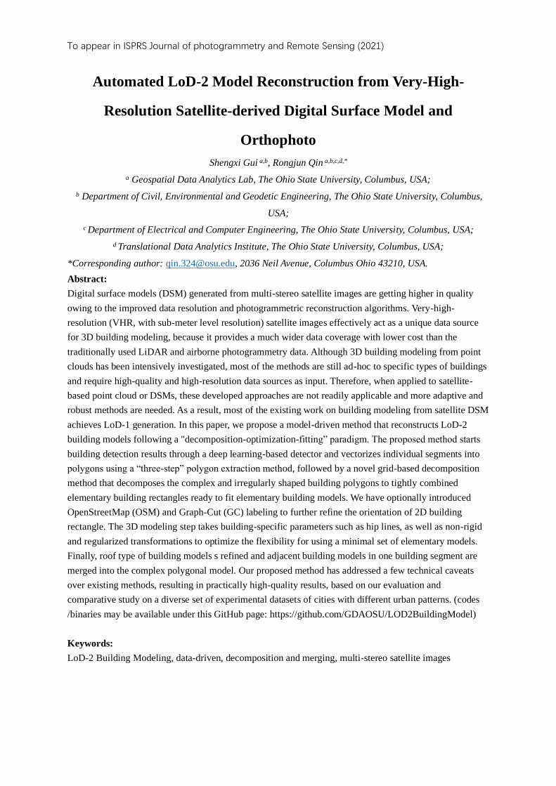
Fig. 1 presents the workflow of our method. We follow the typical reconstruction paradigm as

introduced in Section 2, with a produced DSM and Orthophoto (pre-processing), the process consists of six

main steps: 1) building segmentation, 2) building polygon extraction, 3) building rectangle decomposition,

4) orientation refinement, 5) 3D model fitting, and 6) model post-refinement. The input data of our method

is DSM and the corresponding orthophoto, which is generated by using a workflow based on RPC stereo

processor (RSP) that includes sequentially a level 2 rectification, geo-referencing, point cloud generation,

DSM resampling, and orthophoto rectification (Qin, 2016). The building segmentation from orthophoto is

developed using a combined U-Net based semantic labeling and Mask R-CNN segmentation algorithm. To

extract building polygon, we propose a novel method that first detects the rough boundary of building

segments using the Douglas–Peucker algorithm and then adjusts and regularizes the boundary lines

combining orientation from LSD. Next, to generate and decompose the basic 2D building model from

building polygon, especially in the polygon with several individual small buildings, a novel grid-based

decomposition method is developed to generate and post-process the building rectangles with serval sub-

rectangles in a building segment. The building rectangles are subject to an orientation refinement process

using GC optimization and optionally a rule-based adjustment using OpenStreetMap (OSM). LOD-2

model reconstruction is performed by fitting the most appropriate roof model in a building model library

by optimizing the shape parameters that yield minimum RMSE with the original DSM. In the last step,

model roof type is refined using GC optimization, and simple building models are merged as complex

models based on a few heuristics. The detailed components of each step are given in the following sections.


Fig. 1. Workflow of our proposed method, each key component is described in subsections in the texts.

3.1. Building detection and segmentation

We used an approach that combines two baselines as introduced in Section 2: the U-Net and Mask R-

CNN. U-Net (Ronneberger et al., 2015) with its structure designated for preserving details, provides well-

delineated boundaries of objects, while Mask R-CNN (He et al., 2017) with its original structure, although

less complex to preserve good boundaries, has the ability to perform instance-level segmentation thus often

to have better recall, while given the nature of the region-based detection for Mask R-CNN, it may omit

certain large-sized buildings. These two are complementary to each other, therefore we perform a

segmentation-level fusion for results generated by both networks (introduced in Section 3.1.3). In the

following sections, we introduce training details of U-Net, in which we used a revised loss (Qin et al.,

2019), and the Mask R-CNN, both of which are trained using satellite datasets.

bookmark://Section2/


3.1.1 Semantic labeling based on U-net

We used the training dataset provided by John's Hopkins University Applied Physics Lab's (JHUAPL)

through the 2019 IEEE GRSS Data Fusion Contest (Le Saux et al., 2019). In total, five classes are

considered in this data: ground, tree, roof, water, and bridge and elevated road. While in practice, those

five objects are not balanced, so the number of training patches is adjusted to make the number of each

category have similar patches (Qin et al., 2019).

For the data preparation of training, to improve the training samples, each image with a size of 1024 ×

1024 pixels was split into 512 × 512 patches with 50% overlap. Thus, for each image of 1024 × 1024, 9

patches are available for semantic segmentation so that the training samples are nine times larger than the

original samples.

The loss for this network is defined as dynamic and class-weighted, to adjusts weights of five classes

based on their number of pixels during the process in the individual patch. The weight is computed as:

𝑊𝑖 = 𝑁𝑐 ∙ (1 − 𝑛𝑖

𝑁 ) ( 1 )

where 𝑊𝑖 means the loss weight for class 𝑖, 𝑁𝑐 represents the number of class, 𝑛𝑖 is the number of pixels in

the current patch, and 𝑁 is the total valid pixels in the current patch.

For the prediction part, the data splitting and fusion method are performed as well. The original

testing images with a size of 1024 × 1024 are divided into 512 × 512 patches with 80% overlap. Moreover,

four predictions are performed by rotating the patches into four directions for each patch. The final

prediction can be derived by fusing these predictions with the following strategy: the size of each patch is

512*512, a buffer with a width of 64 pixels in the patch border will not be considered (weight = 0),

otherwise pixels will have a weight equal to 1. In the merging process, a voting strategy is used to calculate

the summed weight of each patch (predictions of four directions are rotated to the original direction), and

the class of pixels will be assigned as the class with the highest weight in that pixel. Thus, the

segmentation result can be developed from orthophotos.

3.1.2 Mask R-CNN building detection

The only category we need is building, and this group is masked for training, validating, and testing.

The vertexes of building masks in samples are extracted using the building polygon extraction method,

described in Section 3.2 and Section 3.3. Furthermore, the bounding-boxes are generated from these

vertexes as well.

In the study, the pre-train weight focus on building segmentation provided by CrowdAI (Mohanty,

2018) is used to Mask R-CNN processing. Furthermore, the dataset of 2019 IEEE GRSS Data Fusion

Contest (Le Saux et al., 2019) is used for training and validation, to achieve a specific weight of network

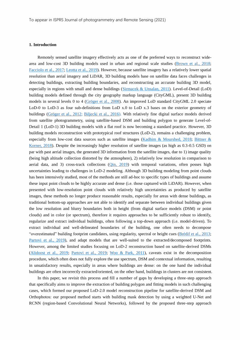
for building segments of orthophoto. During the training step, a total number of 120 epochs training has

been performed, with 30 epochs for RPN training, 60 epochs for FCN training, and 30 epochs for all layers.

Thus, each epoch contains 500 training steps and 50 validation steps. Fig. 2 shows the training process for

Mask R-CNN for a different component of the loss. There is a small disturbance in the epoch of 30

(between RPN training and FCN training), and it remains stably decreasing afterward. On the other hand,

in the validation part, only RPN loss slightly increase, and the other losses include Mask R-CNN loss still


remain decreasing with respect to the training loss.

For the prediction part, the data splitting and fusion method are performed as well. The original

testing images with a size of 1024 × 1024 are divided into 512 × 512 patches. Moreover, the entire

segmentation is developed by merging the segment of the individual patch.

Fig. 2. The relationship between epochs and Mask R-CNN loss for training and validation

3.1.3 Building segmentation fusion

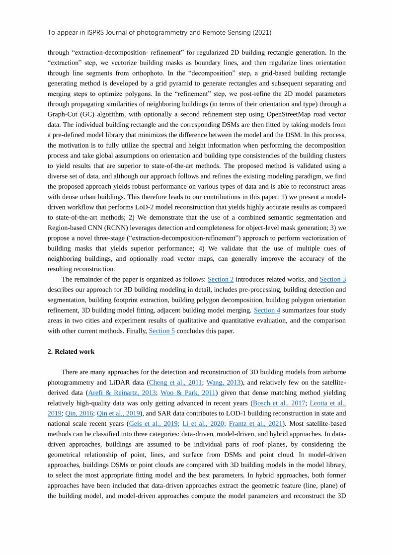
As mentioned above (a schematic workflow is shown in Fig. 3), we used a segmentation-level fusion

to obtain the initial building masks. The fusion method is rather heuristic, as U-Net tends to produce sharp

object boundaries and Mask R-CNN tends to capture individual objects. Therefore, we start by using the

U-Net result as the primary segmentation and use a decision weight 𝑤 to decide if the label of a segment

from Mask R-CNN needs to be used for replacing the result of UNet, as shown below:

𝑤 =1

𝑎𝑟𝑒𝑎𝑏𝑏𝑜𝑥∙

𝑎𝑟𝑒𝑎𝑐𝑙𝑎𝑠𝑠

𝑎𝑟𝑒𝑎𝑏𝑏𝑜𝑥=

𝑎𝑟𝑒𝑎𝑐𝑙𝑎𝑠𝑠

(𝑎𝑟𝑒𝑎𝑏𝑏𝑜𝑥)2 (2)

where 𝑤 indicates the decision weight of a bounding box, 𝑎𝑟𝑒𝑎𝑐𝑙𝑎𝑠𝑠 is the area of the masked pixel cover

in the bounding box, 𝑎𝑟𝑒𝑎𝑏𝑏𝑜𝑥 is the area of the bounding box. The rationale of this formulation follows

the observation that the Mask R-CNN tends to perform well with smaller buildings (possibility due to a

large number of small buildings in the training set), and as long as detection has a good filling within its

bounding box, it may be used as a confident detection of individual buildings. The determination threshold

is empirical (here we variably used 0.1 to 0.2 to yield reasonable results for this 0.5 m resolution data),

which is stable in one region. If the average size is large, the threshold will be close to 0.1. Otherwise, the

threshold will be close to a larger value. , shows the decision process. Firstly, use the semantic labeling

result as primary classification. Secondly, calculate the segment weight of each segment from Mask R-

CNN result, select segments with weight exceeding threshold as potential segments. Finally, use the

potential segments in Mask R-CNN result to replace the corresponding mask of semantic labeling result. 3,

shows the decision process. Firstly, use the semantic labeling result as primary classification. Secondly,

calculate the segment weight of each segment from Mask R-CNN result, select segments with weight

bookmark://Fig2/


exceeding threshold as potential segments. Finally, use the potential segments in Mask R-CNN result to

replace the corresponding mask of semantic labeling result.

Fig. 3. A schematic workflow for segmentation-level fusion

3.2 Initial 2D building polygon extraction

Building polygon extraction aims to vectorize building boundaries as polylines to assist regularized

building model fitting. These polylines need to follow constraints as man-made architectures do, such as

complying with orthogonality and parallelism. For coarse resolution data, this is simplified as polylines

consisting of parallel or orthogonal lines, the extraction of which in this work follows three steps: initial

line extraction, line adjustment, and regularization; the result of each step by example is shown in Fig. 4.

The initial line extraction is performed with well-known Douglas–Peucker algorithm (Douglas &

Peucker, 1973). It starts at the boundary points of the building mask and extracts lines recursively. Due to

the irregularity of the building masks, the initial line segments present errors, sharp angles and are short.

The line adjustment process aims to use the concept of main orientations to connect and turn these short

line segments into consistently long and straight lines: One or more main orientations are defined for the

polygon to separate fitted lines into bins presenting orthogonal lines pairs. First, we draw a histogram of

orientations varying from 0° to 90° with 10° of the interval, and each bin presents two angles that are 90°

different: for example, for the bin present 30°, it would include line segments close to -60° as well. This is

to facilitate maximizing the line adjustment to contain mainly orthogonal and parallel lines for regularity.

Then we sum up the length of lines for each bin and select the bins whose summed length is bigger than a

given threshold (here we set 120 pixels), in which we conclude the main orientation by taking the weighted

average (weight being the length of each segment) of the orientations in that bin. The orientation for the

bin is computed as the weighted average of lines’ orientation in this group (Note: orthogonal orientations

are deemed identify thus only represented by angles within 0°-90°). The adjustment is made by iterating

through each line segment, reassigning to the closest main orientation, intersect and reconnect with

neighboring segments; clear differences can be noted in Fig. 4(a) and Fig. 4(b).

The line regularization process further optimizes line orientation by utilizing detected lines from the

orthophoto: Line-Segment Detector (LSD) algorithm (Von Gioi et al., 2010) is used to extract line

segments and the orientation of each line segment is used to readjust orientations of the nearest line of the

initially extracted line segments from the building mask to enable consistencies between the detected


footprint and the image edges. The resulting building footprint after this process is regarded as the initial

building polygon for reference.

(a) (b) (c)

Fig. 4. Two examples are showing boundary extraction of building polygon. (a) boundary after initial line

extraction; (b) boundary after line adjustment; (c) boundary after line regularization.

3.3. A grid-based rectangle decomposition algorithm for building rectangles

The polyline based initial building polygon can be overcomplex for the limited number of simplex

models to fit, thus it requires to decompose these building polygons (as produced following method

introduced in Section 3.2), into simple shapes, which in this work as basic rectangles on which the model

fitting can base on (we call it building rectangle hereafter). Existing methods mostly follow a greedy

strategy for decomposition, which identifies the main orientation following the longest straight line,

extends parallel lines gradually to get decomposed rectangles to fill the polygon (Kada, 2007; Partovi et al.,

2019). However, often the results of such a greedy-decomposition method do not match the actual building

components. We therefore present our grid-based decomposition approach, in which can be flexibly

integrated information from the orthophoto and DSMs to guide this process.

The grid-based decomposition approach assumes that multicomplex building polygons generally

follow the Manhattan type and are composed of simplex rectangles, the seamlines of which can be

approximately either horizontal or vertical on a 2D grid. The workflow is shown in Fig. 5. To start, we

first rotate the 2D building polygon by aligning its main orientation to the x-axis (Fig. 5), and the same

transformation will be performed on the Orthophoto and DSM. The decomposition of the polygon to

rectangles starts with a DSM and orthophoto based initial decomposition: first, gradients of the DSM in

both the horizontal and vertical directions are computed and the those larger than a threshold (0.3 m),

followed by a non-maximum suppression (with a window size of 7 pixels) are selected as the candidate of

lines for separating the polygon, which is further filtered by considering the color information: for each

candidate separating line, we create a small buffer on both side and only lines with color differences of

between these two buffers bigger than a threshold Td (we used 10 for an 8-bit image). For the segments

after this initial decomposition, a maximum inner rectangle extraction (Alt et al., 1995) is performed to

extract individual rectangles. Note this above process is performed on the coarsest layer of an image

pyramid to reduce impacts of the noise, and the results are then interpolated to the finer layers for further

analysis. We kept three layers for our 0.5m resolution data, (grid level 1-3, Fig. 5), meaning that the top


layer is ¼ of the original resolution.

The individual rectangles will then be projected to the original resolution grid and post-processed by

using a merging operation, as the above process might over separate the building masks. However,here the

merging operation will only be performed on rectangles that share one edge, as the merged rectangles must

be rectangles as well to enable fitting. To start, we first identify adjacent rectangles by dilating their

boundaries for 7 pixels and define adjacency as long as there are overlaps and the common edge has a

similar length (the difference shorter than 5 pixels in length). The criterion used to decide if two adjacent

rectangles should be merged as below:

{𝑚𝑒𝑟𝑔𝑒, |𝐶1

− 𝐶2 | < 𝑇𝑑 ∩ |𝐻1

− 𝐻2 | < 𝑇ℎ1 ∩ 𝑚𝑎𝑥|∆𝐻𝑒𝑑𝑔𝑒| < 𝑇ℎ2

𝑛𝑜𝑡 𝑚𝑒𝑟𝑔𝑒, 𝑜𝑡ℎ𝑒𝑟𝑤𝑖𝑠𝑒 (3)

meaning that the mean color differences (|𝐶1 − 𝐶2

|) of the two rectangles (projected onto the orthophoto)

is smaller than a threshold Td (here we define as 10 for an 8-bit image); 2) mean height difference (|𝐻1 −

𝐻2 |) is smaller than a threshold Th1 (1 m); 3) There is no dramatic height changes in a buffered region that

cover the common edge, to avoid narrow streets in between, and this criterion is defined as the height

gradient (∆𝐻𝑒𝑑𝑔𝑒) in the overlapped region (after the dilation) smaller than Th2 (0.2 m).

Fig. 5. The proposed grid-based decomposition algorithm. Details are in the texts.

3.4 Orientation refinement for Building rectangles

The rectangular building elements produced based on the process as described above are independent

of each other, and on the other hand, the orientation of these rectangle footprints can be easily impacted by

noises of the initial building mask and the orthophotos & DSM, considering that most neighboring

buildings follow consistent orientations, such as those in the same street block. Therefore, we optimize the

orientations for buildings using the Graph-Cut algorithm (Boykov & Jolly, 2001), and as an optional step

to refine the orientation using available OpenStreetMap road networks (covering 80% of the cities

worldwide (Barrington-Leigh & Millard-Ball, 2017)).


3.4.1 Building rectangle orientation refinement by graph-cut labeling

We formulate the orientation adjustment problem as a multi-labeling problem, by assigning each

building rectangle, possible labels as discrete angle values, ranging from 0° to 180°, with a 2° as the

interval, resulting in approximately 90 labels (0° pointing to the north). We aim to assign these labels such

that similar neighboring building rectangles have the same or similar labels, where similarity is defined by

using texture and height differences. GC is well known for solving multi-label problems in polynomial

time (Kolmogorov & Zabih, 2002). It aims to minimize a cost function consisting of data and a smoothness

term, in which the smoothness terms aims to enforce consistency between nodes and the data terms encode

a priori information, shown in

𝐸(ℒ) = ∑ 𝑅(𝑥𝑖 , ℒ𝑖)𝑥𝑖𝜖𝑃 + 𝜆 ∑ 𝐵(𝑥𝑖 , 𝑥𝑗 )(𝑥𝑖, 𝑥𝑗)𝜖ℕ 𝛿(ℒ𝑖 , ℒ𝑗) (4)

𝑅(𝑥𝑖 , ℒ𝑖) = 1 − 𝑒−|𝜃𝑥𝑖−𝜃ℒ𝑖

| (5)

𝐵(𝑥𝑖 , 𝑥𝑗) = 𝑊(𝑖, 𝑗) (6)

𝛿(ℒ𝑖 , ℒ𝑗) = {0, 𝑖𝑓 ℒ𝑖 = ℒ𝑗

1, 𝑖𝑓 ℒ𝑖 ≠ ℒ𝑗 (7)

where ℒ = {0,1,2, . . . ,89} is the label space indicating the orientation of the rectangle being 𝜃ℒ = 2 × ℒ

degrees, and ℒ𝑖 refers to the optimized label (or 𝜃ℒ𝑖 as the optimized orientation) for the building rectangle

𝑥𝑖. 𝜃𝑥𝑖 refers to the initial orientation of the building rectangle and the data term 𝑅(𝑥𝑖 , ℒ𝑖) tends to keep the

initial orientation unchanged and is defined as a normalized value (smaller than 1) that gets bigger as the

optimized orientation differs more. 𝐵(𝑥𝑖 , 𝑥𝑗 ) is the smooth term, which defines the similarity of

neighboring building rectangles (set ℕ ), and 𝜆 is the weight that leverages the contributions of the

smoothness term. The smoothness term 𝐵(𝑥𝑖 , 𝑥𝑗 ) is determined by using affinity matrix 𝑊(𝑖, 𝑗), and

which adapts an exponential kernel (Liu & Zhang, 2004):

𝑊(𝑖, 𝑗) = 𝑒−𝑑𝑖𝑠𝑡(𝑖,𝑗)/2𝜎2 (8)

𝑑𝑖𝑠𝑡(𝑖, 𝑗) = √𝑤𝑟(𝒏𝒓𝒊 − 𝒏𝒓𝒋)

2+ 𝑤𝜃(𝑛𝜃𝑖 − 𝑛𝜃𝑗)

2+ 𝑤𝑆(𝒏𝑺𝒊 − 𝒏𝑺𝒋)

2

+𝑤𝐶(𝒏𝑪𝒊 − 𝒏𝑪𝒋)2

+ 𝑤𝜎(𝒏𝝈𝒊 − 𝒏𝝈𝒋)2 (9)

where 𝑊(𝑖, 𝑗) is the affinity weight matrix for neighboring building rectangle 𝑖 and 𝑗, with 0 < 𝑊(𝑖, 𝑗) <

1, 𝜎 is the bandwidth of exponential kernel. 𝑑𝑖𝑠𝑡(𝑖, 𝑗) is the similarity between building rectangle 𝑥𝑖 and 𝑥𝑗,

calculated as a weighted (and normalized) combination of a few factors including the distance of two

rectangle center 𝒏𝒓𝒊, the difference of the orientation, the shape 𝒏𝑺𝒊, the color 𝒏𝑺𝒊, and that of the color

variations 𝒏𝝈𝒊 , respectively defined as 𝒏𝒓𝒊 = (𝑛𝑋𝑖 , 𝑛𝑌𝑖), where 𝑛𝑋𝑖 and 𝑛𝑌𝑖 referring to the location of

the rectangle center, 𝒏𝑺𝒊 = (𝑛𝐿1,𝑖 , 𝑛𝐿2,𝑖) referring to the length 𝑛𝐿1,𝑖 and width 𝑛𝐿2,𝑖 of the rectangle,

𝒏𝑪𝒊 = (𝑛𝐶𝑅,𝑖 , 𝑛𝐶𝐺,𝑖 , 𝑛𝐶𝐵,𝑖) referring the mean value of RGB that rectangle covers, 𝒏𝝈𝒊 =


(𝑛𝜎𝑅,𝑖 , 𝑛𝜎𝐺,𝑖 , 𝑛𝜎𝐵,𝑖) referring to the standard deviation of RGB. We give a higher weight value 𝑤𝑟 = 3 to

location, to ensure consistencies are mainly optimized locally; the weight of orientation 𝑤𝜃 and the weight

of shape 𝑤𝑆 are set by default as 1, and the weight of RGB color 𝑤𝐶 and the weight of RGB standard

deviation 𝑤𝜎 are set as 0.3, since both the 𝒏𝑪 and 𝒏𝝈 have three components. Note all measures for

computing similarities are normalized through an exponential kernel similar to (8). These weights (for

location, orientation & shape, color-consistency to decide similarity of two neighboring buildings), are set

to be intuitive and often can be fixed in the optimization based on the quality of the data. It is possible to

automatically tune these parameters based on prior information of the dataset with the meta-learning

method, or to decide the parameter based on the distribution of the data (while only slight difference from

our empirical values (Kramer, 1987)). Here since these parameters are intuitive and explainable, these

weights do not proceed an automated tuning.

3.4.2 Building rectangle orientation refinement using OpenStreetMap

OpenStreetMap is a publicly available vector database and it was known to have covered more than

80% (Barrington-Leigh & Millard-Ball, 2017) of the road networks globally, thus it may serve as a valid

source to refine building orientations for the well geo-referenced dataset. We made a simple assumption

that the buildings always have the same direction as their surrounding road vectors (Zhuo et al., 2018).

Therefore, we perform the OSM based orientation refinement following simple heuristics or reassigning

orientation using nearest criterion: for each building rectangle, the nearest road vector is found by

computing the distance between the center of the building rectangle and each road vector, and if the

intersection angle between the main orientation line of a building polygon (introduced in Section 3.2) and

the nearest road vector is smaller than 30°, the orientation of the rectangle will be adjusted, otherwise kept

unchanged. This process will allow minor adjustment of the orientation when the OSM data is available.

Two examples are shown in Fig. 6 as comparisons when the GC optimization and the OSM-based

adjustment are respectively applied, resulting in adjusted rectangles (in blue and green). Once OSM is

unavailable in a certain region or orientation difference between building and OSM street line, orientation

refinement using OSM will not execute and there will be sole refinement by using GC.

(a) (b) (c)

Fig. 6. Two examples showing building rectangle orientation respectively adjusted by GC (b) and OSM (c).


Blue and Green rectangles refer to those changed during the decomposition. (a) shows polygons before the

orientation refinement.

3.5 3D model fitting

The extracted building polygons are in rectangle shapes; together with DSM/nDSM, these can be

easily fitted by simplex building models. Here we only consider five types of building models namely: flat,

gable, hip, pyramid, and mansard, a brief illustration of which is shown in Fig. 7. It can be noted the

complexity of the roof topology increases from left to right, along with more parameters to be considered

for fitting.

(a) (b)

Fig. 7. (a) Model roof library with five types and geometrical parameters, color-coded for subsequent

demonstration of results. (b). Tunable parameters to define these model types.

Each building model can be described by using several geometrical parameters. we adopt the

parameterization based on (Partovi et al., 2019), where the geometrical parameters 𝜓 are defined as

follows:

𝜓 ∈ 𝚿; 𝚿 = {𝑷, 𝑪, 𝑺} (10)

where Ψ includes three subsections, 𝑃, 𝐶, 𝑆. With 𝑷 = {𝑥0, 𝑦0, 𝑂𝑟𝑖𝑒𝑛𝑡𝑎𝑡𝑖𝑜𝑛} are the location parameters of

the building model, and 𝑪 = {𝑙𝑒𝑛𝑔𝑡ℎ, 𝑤𝑖𝑑𝑡ℎ} are the contour parameters of the building model, and 𝑺 =

{𝑍𝑟𝑖𝑑𝑔𝑒 , 𝑍𝑒𝑎𝑣𝑒 , ℎ𝑖𝑝𝑙, ℎ𝑖𝑝𝑤} are the shape parameters of the building model, and the geometrically meaning

of these parameters are shown in Fig. 7 (b). Each type of building model may be special cases for this type

(shown in Fig. 7): for example: for flat building 𝑍𝑟𝑖𝑑𝑔𝑒 = 𝑍𝑒𝑎𝑣𝑒, and for hip building, ℎ𝑖𝑝𝑤 = 𝑤𝑖𝑑𝑡ℎ/2

etc. Details of different models under this rationale can be found in Table 1, where “width”, “length” come

from the fitted polygons, and “Height ” is calculated as the mean elevation (from DSM) based on the

building polygon (i.e. rectangle).

Table. 1. Initial parameters of the building model, parameters with * means these are constants

Model type hipl(0) hipw(0) Zeave(0) Zridge(0)

Flat building 0∗ 0∗ Height − 0.5 m Height − 0.5 m

Gable building 0∗ 1/2 width∗ Height − 0.5 m Height

Hip building 1/4 length 1/2 width∗ Height − 0.5 m Height

Pyramid building 1/2 length∗ 1/2 width∗ Height − 0.5 m Height

Mansard building 1/4 length 1/4 width Height − 0.5 m Height

The optimization specifically updates the parameter set 𝑺 = {𝑍𝑟𝑖𝑑𝑔𝑒 , 𝑍𝑒𝑎𝑣𝑒 , ℎ𝑖𝑝𝑙, ℎ𝑖𝑝𝑤} based on the

DSM, where the starting terrain height is computed by taking the local minimum of building height. Given

the noisiness of the DSM, we consider directly perform an exhaustive search over the parameters set and

choose the model and parameter set with the smallest RMSE. As can be seen from Table 1, the enabled

parameters for exhaustive search increase as the model get more complex. We observe that since one


building only covers a few hundreds of pixels, even with exhaustive search, the computational time is still

reasonable to scale up. Ranges of parameters for searching are shown in Table 2, the value of “searching

step size” decided by the resolution of satellite-derived DSM (0.5-meter ground sampling distance (GSD)).

Table. 2. Optimization parameters with their range and step

Parameter Parameter range Searching step size

Zeave (Zeave(0) − 3, Zeave(0) + 3) 0.2

Zridge (Zeave + 0.5, Zeave + 4) 0.2

Hipl (hipl(0) − 1/8 length, hipl(0) + 1/8 length) 0.4

Hipw (hipw(0) − 1/8 width, hipw(0) + 1/8 width) 0.4

3.6 Model post-refinement

3.6.1 Enforcing building type consistency

Since the type of models are individually fitted and the nosiness of the DSM may result in

inconsistent types of building for neighboring and similar building objects (an example shown in Fig. 8(a)).

Here we use the same idea to enforce the consistencies of the building types through GC optimization

(details in Section 3.4.2), in which label space contains five labels representing the used building types,

and the smooth term 𝐵(𝑥𝑖 , 𝑥𝑗) keeps the same (Equation (6) ~ (9)) as to enforce label consistency for

neighboring buildings with similar color and height, and the data term 𝑅 (𝑥𝑖 , ℒ𝑖

′) for building type follows

a binary representation being a constant if the target label equals to the initial label, otherwise a large

number:

𝐸 (ℒ ′) = ∑ 𝑅 (𝑥𝑖 , ℒ𝑖

′)𝑥𝑖𝜖𝑃 + 𝜆 ∑ 𝐵(𝑥𝑖 , 𝑥𝑗 )(𝑥𝑖, 𝑥𝑗)𝜖ℕ 𝛿 (ℒ

𝑖

′, ℒ

𝑗

′) (11)

𝑅 (𝑥𝑖 , ℒ𝑖

′) = 1 − 𝑒

−𝐷(𝑥𝑖,ℒ𝑖

′) (12)

𝐷 (𝑥𝑖 , ℒ𝑖

′) = {

0, 𝑇𝑦𝑝𝑒𝑥𝑖= 𝑇𝑦𝑝𝑒

ℒ𝑖

′

1, 𝑇𝑦𝑝𝑒𝑥𝑖≠ 𝑇𝑦𝑝𝑒

ℒ𝑖

′ (13)

where ℒ ′ = {𝑓𝑙𝑎𝑡, 𝑔𝑎𝑏𝑙𝑒, ℎ𝑖𝑝, 𝑝𝑦𝑟𝑎𝑚𝑖𝑑, 𝑚𝑎𝑛𝑠𝑎𝑟𝑑} is the label space indicating the building type of the

rectangle for type refinement, and ℒ𝑖

′ refers to the optimized label (same as 𝑇𝑦𝑝𝑒

ℒ𝑖

′) for building rectangle

𝑥𝑖. 𝑇𝑦𝑝𝑒𝑥𝑖 refers to the initial building type of building rectangle and the data term 𝑅 (𝑥𝑖 , ℒ

𝑖

′) tends to

remain the same type as initial, the value of which is normalized using an exponential kernel. Data term

𝑅 (𝑥𝑖 , ℒ𝑖

′) is determined by a binary function 𝐷 (𝑥𝑖 , ℒ

𝑖

′), representing the building type difference between

building rectangle 𝑥𝑖 and potential label ℒ𝑖

′, and it is set as zero if the building types are the same as the

initial type.


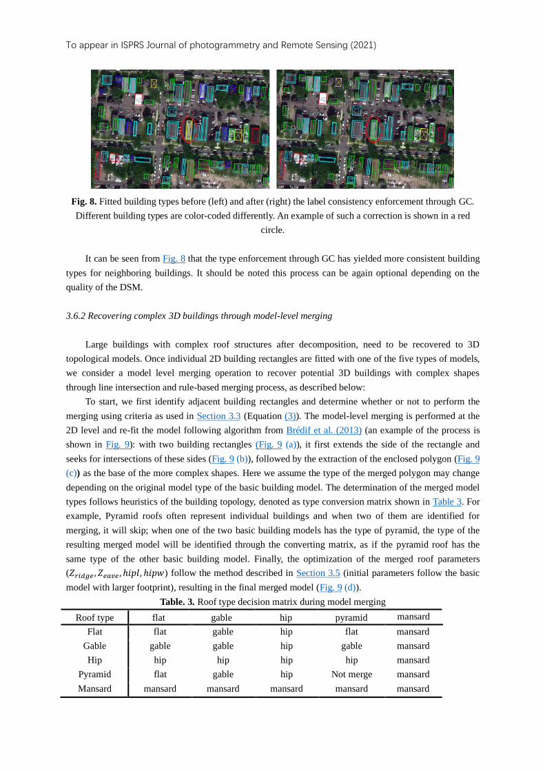
Fig. 8. Fitted building types before (left) and after (right) the label consistency enforcement through GC.

Different building types are color-coded differently. An example of such a correction is shown in a red

circle.

It can be seen from Fig. 8 that the type enforcement through GC has yielded more consistent building

types for neighboring buildings. It should be noted this process can be again optional depending on the

quality of the DSM.

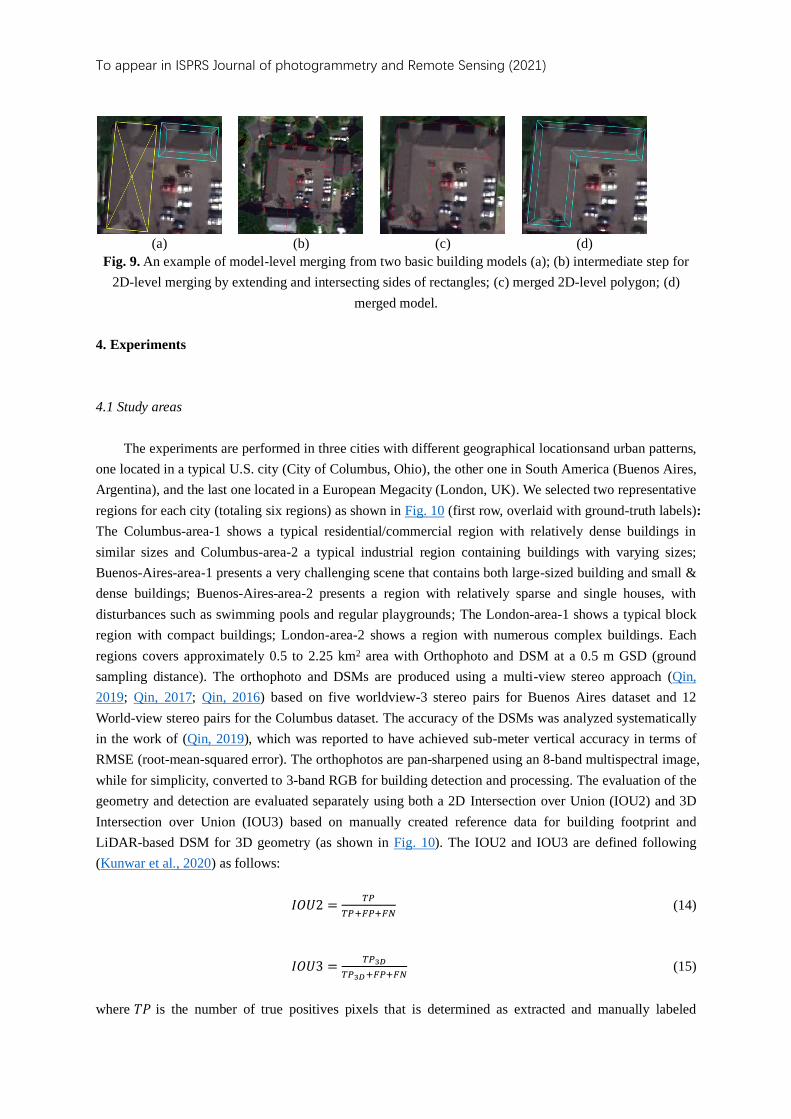
3.6.2 Recovering complex 3D buildings through model-level merging

Large buildings with complex roof structures after decomposition, need to be recovered to 3D

topological models. Once individual 2D building rectangles are fitted with one of the five types of models,

we consider a model level merging operation to recover potential 3D buildings with complex shapes

through line intersection and rule-based merging process, as described below:

To start, we first identify adjacent building rectangles and determine whether or not to perform the

merging using criteria as used in Section 3.3 (Equation (3)). The model-level merging is performed at the

2D level and re-fit the model following algorithm from Brédif et al. (2013) (an example of the process is

shown in Fig. 9): with two building rectangles (Fig. 9 (a)), it first extends the side of the rectangle and

seeks for intersections of these sides (Fig. 9 (b)), followed by the extraction of the enclosed polygon (Fig. 9

(c)) as the base of the more complex shapes. Here we assume the type of the merged polygon may change

depending on the original model type of the basic building model. The determination of the merged model

types follows heuristics of the building topology, denoted as type conversion matrix shown in Table 3. For

example, Pyramid roofs often represent individual buildings and when two of them are identified for

merging, it will skip; when one of the two basic building models has the type of pyramid, the type of the

resulting merged model will be identified through the converting matrix, as if the pyramid roof has the

same type of the other basic building model. Finally, the optimization of the merged roof parameters

(𝑍𝑟𝑖𝑑𝑔𝑒 , 𝑍𝑒𝑎𝑣𝑒 , ℎ𝑖𝑝𝑙, ℎ𝑖𝑝𝑤) follow the method described in Section 3.5 (initial parameters follow the basic

model with larger footprint), resulting in the final merged model (Fig. 9 (d)).

Table. 3. Roof type decision matrix during model merging

Roof type flat gable hip pyramid mansard

Flat flat gable hip flat mansard

Gable gable gable hip gable mansard

Hip hip hip hip hip mansard

Pyramid flat gable hip Not merge mansard

Mansard mansard mansard mansard mansard mansard


(a) (b) (c) (d)

Fig. 9. An example of model-level merging from two basic building models (a); (b) intermediate step for

2D-level merging by extending and intersecting sides of rectangles; (c) merged 2D-level polygon; (d)

merged model.

4. Experiments

4.1 Study areas

The experiments are performed in three cities with different geographical locationsand urban patterns,

one located in a typical U.S. city (City of Columbus, Ohio), the other one in South America (Buenos Aires,

Argentina), and the last one located in a European Megacity (London, UK). We selected two representative

regions for each city (totaling six regions) as shown in Fig. 10 (first row, overlaid with ground-truth labels):

The Columbus-area-1 shows a typical residential/commercial region with relatively dense buildings in

similar sizes and Columbus-area-2 a typical industrial region containing buildings with varying sizes;

Buenos-Aires-area-1 presents a very challenging scene that contains both large-sized building and small &

dense buildings; Buenos-Aires-area-2 presents a region with relatively sparse and single houses, with

disturbances such as swimming pools and regular playgrounds; The London-area-1 shows a typical block

region with compact buildings; London-area-2 shows a region with numerous complex buildings. Each

regions covers approximately 0.5 to 2.25 km2 area with Orthophoto and DSM at a 0.5 m GSD (ground

sampling distance). The orthophoto and DSMs are produced using a multi-view stereo approach (Qin,

2019; Qin, 2017; Qin, 2016) based on five worldview-3 stereo pairs for Buenos Aires dataset and 12

World-view stereo pairs for the Columbus dataset. The accuracy of the DSMs was analyzed systematically

in the work of (Qin, 2019), which was reported to have achieved sub-meter vertical accuracy in terms of

RMSE (root-mean-squared error). The orthophotos are pan-sharpened using an 8-band multispectral image,

while for simplicity, converted to 3-band RGB for building detection and processing. The evaluation of the

geometry and detection are evaluated separately using both a 2D Intersection over Union (IOU2) and 3D

Intersection over Union (IOU3) based on manually created reference data for building footprint and

LiDAR-based DSM for 3D geometry (as shown in Fig. 10). The IOU2 and IOU3 are defined following

(Kunwar et al., 2020) as follows:

𝐼𝑂𝑈2 =𝑇𝑃

𝑇𝑃+𝐹𝑃+𝐹𝑁 (14)

𝐼𝑂𝑈3 =𝑇𝑃3𝐷

𝑇𝑃3𝐷+𝐹𝑃+𝐹𝑁 (15)

where 𝑇𝑃 is the number of true positives pixels that is determined as extracted and manually labeled


building footprint simultaneously, 𝐹𝑃 is the number of false positives and 𝐹𝑁 is the number of false

negatives. 𝑇𝑃3𝐷 is 𝑇𝑃 pixels whose 3D vertical difference from the ground-truth LiDAR is within 2 m.

Fig. 10. First row: Orthophotos of the study areas, overlaid with manually drawn masks; second row:

corresponding ground-truth LiDAR data.

4.2 Experimental results

The orthophotos study areas are shown in Fig. 10, first row, overlaid with manually drawn building

masks results of the building 2D polygon and rectangle extraction (methods described in Section 3.1-3.4)

and building 3D model fitting (methods described in Section 3.5-3.6) are shown in Fig. 11, which

specifically includes building mask detection, initial building polygon detection, decomposition & merging,

and orientation refinement with GC and OSM. We show the model fitting results of the six experimental

regions in the first row of Fig. 11, by projecting the wireframes of the model on the orthophoto; in the

second row of Fig. 11, we demonstrate intermediate results of the first region (i.e. Columbus-area-1)

including initial building polygon extraction, building rectangle decomposition and refinement, as well as

the final fitted more, with the third row of Fig. 11 highlighting some of the results. It can be seen that the

proposed method has detected most of the buildings and correctly outlined the building boundaries. In

addition, most of the buildings initially detected to be connected are successfully decomposed as individual

rectangles. Minor errors are observed for small and complex buildings where decompositions may fail: an

example is shown in the third row (circled in red), which has erroneously separated buildings into a thin

rectangle thus being reconstructed incorrectly.

Fig. 11 also shows the final result of building modeling for the six regions with roof type, and classes

other than building are set as terrain DSM. Fig. 12 display the LoD-2 reconstructed buildings in six

experimental areas. The result indicates that the proposed approach performs well on community building

in Columbus-area-1, Columbus-area-2, and Buenos-Aires-area-2, while in extraordinarily complex blocks,

like Buenos-Aires-area-1 and London-area-1, some buildings are not reconstructed so accurate, since

building mask from Section 3.1 does not detect perfect segments.


Fig. 11. LoD-2 model reconstruction steps for Columbus-area-1. First row: Intermediate results of the

“Columbus-area-1” region including initial building polygon extraction, polygon decomposition and

refinement, model fitting and the last figure of this row shows the 3D visualization. The second row

enlarges part of each figure of the second row for visualization. The building circled in red shows an

example of erroneous reconstruction.


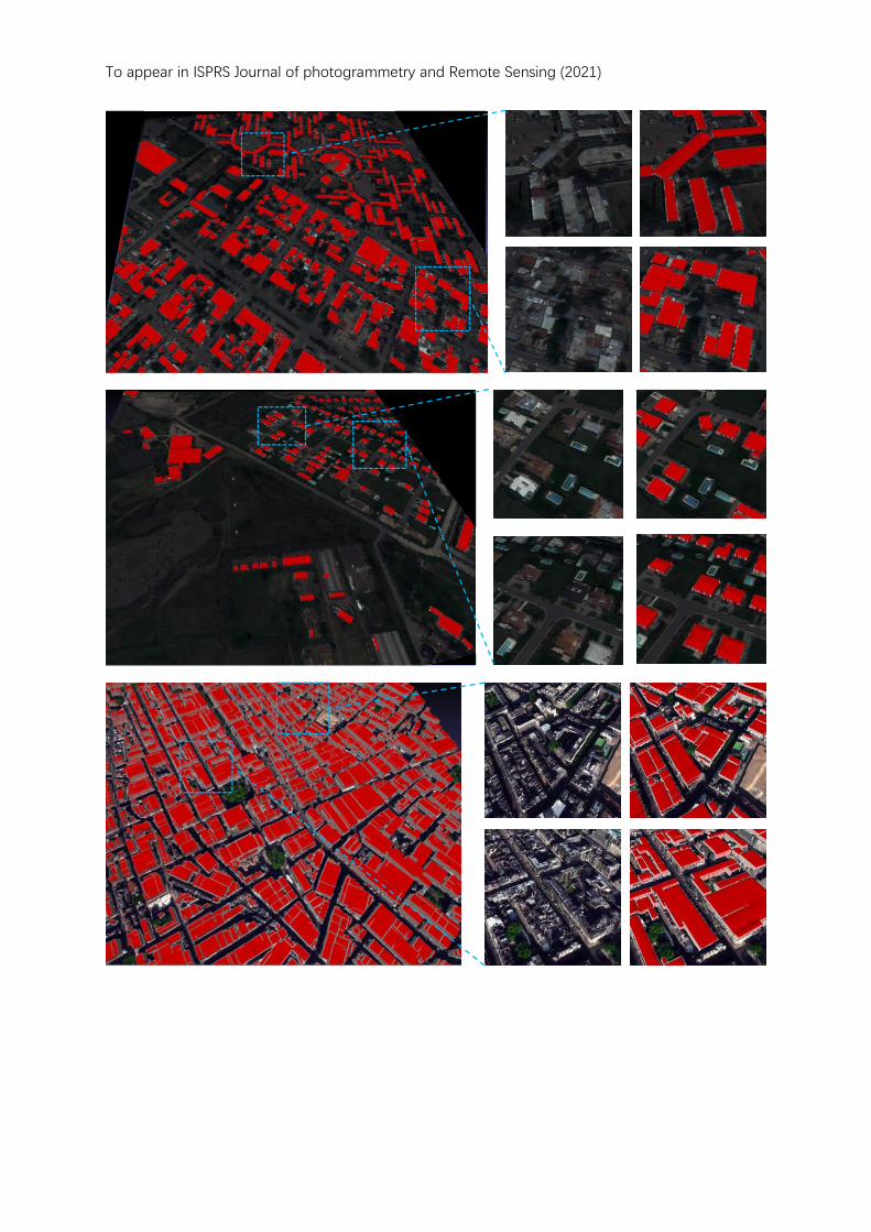
Fig. 12. LoD-2 model reconstruction results of the six experimental regions. Left column: 3D model with

roof covered by red mask and façade covered by white; medium column: DSM with texture in a close view,

right column: 3D model with roof covered by red mask in a close view. From top to bottom: Columbus-

area-1, Columbus-area-2, Buenos-Aires-area-1, Buenos-Aires-area-2, London-area-1, and London-area-2.

4.3 Accuracy evaluation of experiment areas

The accuracy of the resulting models is evaluated using the IOU2 and IOU3 metrics, respectively to

assess the 2D building footprint extraction accuracy and the 3D fitting accuracy. The accuracy of ‘DSM’

represents the raw measurements to be compared with the ground truth. We have ablated the results with

and without the GC and OSM refinements, statistics against the ground truth are shown in Table 4, where

“OSM” or “GC” indicates that the orientation is refined using OSM or GC alone, and “OSM+GC”

indicates the orientation being refined by OSM first and followed by GC. Notable examples are shown in

Fig. 13, the first two rows of which indicated that the OSM might be able to correct orientations of

buildings, while do not influence cases if orientations of the buildings are already well-estimated (third

row of Fig. 13). In both cases, OSM and GC refinement had a positive impact on the resulting metrics in

three out of the six areas, and it is possible that incorrect OSM might adversely impact the final IOU. It

should be noted that although the statistics show only a marginal improvement of the GC and OSM

refinement (largely due to that these adjustments are small and the building segments are rather accurate),

it visually shows a much better consistency in occasions where the buildings are misoriented (e.g. Fig. 6).

The fitted DSM has a larger error distribution than the original DSM, since often fitting will result in

reduced accuracy given that the regularized shape may introduce errors, as for example, a raw

measurement curved surface may be approximated by multiple pieces of a planar surface, and the same

applies to the model fittings.


Fig. 13. Building model height result with different orientation refinement options. The red circled regions

highlight notable differences among different strategies.

Table. 4. Accuracy evaluation of the resulting building models

Region Accuracy DSM No

refinement OSM GC OSM+GC

Columbus area 1

IOU2 0.6929 0.6348 0.6359 0.6349 0.6362

IOU3 0.6632 0.5780 0.5794 0.5782 0.5796

Columbus area 2

IOU2 0.8360 0.8076 0.8084 0.8076 0.8085

IOU3 0.8287 0.7950 0.7961 0.7951 0.7962

Buenos Aires area 1

IOU2 0.6709 0.6378 0.6377 0.6380 0.6381

IOU3 0.6551 0.5892 0.5888 0.5893 0.5894

Buenos Aires area 2

IOU2 0.3539 0.5301 0.5298 0.5302 0.5301

IOU3 0.3281 0.4829 0.4825 0.4828 0.4827

London area 1

IOU2 0.6830 0.5797 0.5799 0.5796 0.5798

IOU3 0.6176 0.4711 0.4714 0.4707 0.4712

London area 2

IOU2 0.6004 0.5053 0.5052 0.5048 0.5052

IOU3 0.5626 0.4180 0.4180 0.4160 0.4163

4.4 Comparative study

We compare our results with results generated by state-of-the-art methods, and given the nature of the

LoD-2 model reconstruction method being component-rich, trivial and often ad-hoc, we re-implement and

compare the key components of some of the existing methods on their algorithms for building polygon

extraction and decomposition, these methods being: the method in (Partovi et al., 2019), (Wei et al., 2020),

(Arefi & Reinartz, 2013), and that in (Li et al., 2019). The two key components we are comparing against

existing methods are: 1) building polygon extraction (process described in Section 3.2), and 2) building

polygon decomposition (process described in Section 3.3). The building polygon extraction methods

include 1) a generalization of line segments-based building outline extraction method (Partovi et al., 2019),

which generates building mask by applying SVM classification to gradient feature from PAN image and

extract primitive boundary points by using SIFT algorithm (Lowe, D. G, 2004), and then fit boundary line

segments from points and regularized them by finding building’s orientation; 2) a toward automatic

building footprint delineation by using CNN and regularization method (Wei et al., 2020), which firstly

segments buildings via FCN with multiple scale aggregation of feature pyramids from convolutional layers,

and next regularizes polygon by adapting a coarse and fine polygon adjustment; 3) a minimum bounding

rectangle (MBR) based method (Arefi & Reinartz, 2013), which approximates the remaining polygon by


calculating bounding rectangle of building segment and the difference mask between bounding rectangle

and building mask, with MBR-based algorithm for rectilinear building and RANSAC-based approximation

algorithm for non-rectilinear building. The rectangle decomposition methods include 1) a parallel line-

based building decomposition method (Partovi et al., 2019), which moves line segments until it meets the

buffer of another parallel line segment and then generates rectangles using these two parallel line segments;

2) a primitive-based 3d building modeling method (Li et al., 2019), which cascades a building into a set of

parts via mask R-CNN, and uses a greedy approach to select and move instance with largest IOU to

decompose the building into a set of shapes. To ensure that the performance of building polygon extraction

methods and rectangle decomposition method are evaluated individually, the comparison is designed as

that polygon extraction methods share the same building mask input from Section 3.1, and rectangle

decomposition methods share the same building polygon from Section 3.2 and IOU2 is used as the metric

for evaluation. The building polygon extraction from (Partovi et al., 2019) was realized using the SIFT

algorithm to detect key points and those points are selected as boundary points only around the building

mask from Section 3.1. For (Wei et al., 2020) and (Arefi & Reinartz, 2013), primitive building segment is

replaced by using building mask from Section 3.1.

Fig. 14 shows the sample result of all methods for building polygon extraction, Fig. 15 shows the

sample result of all methods for building polygon decomposition to building rectangles, and Table 5 gives

the statistics. It can be seen that our method in both of the tasks outperforms all the existing methods,

especially in Fig. 14-15, our methods due to the nature of deeply integrating decision criteria on the image

color similarity and DSM continuity through a grid-based approach, the detection and decomposition

algorithms are able to identify regularized polylines, and identify separating boundaries for building

rectangles. Compared to all other existing approaches, either miss detections or incorrectly locate or

identify building rectangles. Examples showing the limitation of our method can be found in Fig. 15, the

last row, in which our method has failed to separate a connected building and created a minor artifact due

to shadows, whereas other methods in this example are found to be worse in decomposition. Table 5 shows

that among the six regions we have experimented on, the IOU2 of our results achieves the highest for both

tasks, except for Buenos-Aires-area 2 and London-area 2, which is marginally lower.


Fig. 14. Comparative results on building polygon extraction with other state-of-the-art methods.

Table. 5. IOU2 values of comparing results in building footprint extraction and decomposition (Bold

values indicate the best performing approach and italic the second best)

Method Columbus

area1 Columbus

area2 Buenos

Aires area 1 Buenos

Aires area 2 London area 1

London area 2

Building Polygon

Extraction

(Partovi, 2019) 0.6827 0.8157 0.6456 0.6109 0.6623 0.5744

(Wei, 2020) 0.6811 0.8179 0.6543 0.6093 0.6601 0.5765

(Arefi, 2013) 0.6433 0.7761 0.5381 0.5778 0.4545 0.4639

Ours 0.6831 0.8195 0.6549 0.6099 0.6624 0.5749

Rectangle Decomposition

(Partovi, 2019) 0.6579 0.7679 0.5976 0.5532 0.5745 0.4848

(Li, 2019) 0.5768 0.7618 0.5980 0.5533 0.5781 0.5110

Ours 0.6587 0.8133 0.6375 0.5969 0.5796 0.5136


Fig. 15. Comparative results on building polygon decomposition with other state-of-the-art methods.

4.5 Parameter analysis

With several tunable parameters in the proposed approach, it is worth discussing the sensitivity of the

parameters in Table 6. All five thresholds listed in Table. 6 contribute to the 2D building shape in the

approach, and are assigned based on the empirical studies in the experiment. Two areas in Columbus are

taken to analyze the impact of each threshold. A pair of initial thresholds are separately assigned to those

two experimental areas, with 𝑻𝟏 = {𝑇𝑤 , 𝑇𝑙 , 𝑇𝑑 , 𝑇ℎ1 , 𝑇ℎ2 } = {0.16,120,10,1,0.2} for Columbus-area-1 and

𝑻𝟐 = {𝑇𝑤 , 𝑇𝑙 , 𝑇𝑑 , 𝑇ℎ1, 𝑇ℎ2 } = {0.2,120,10,1,0.2} for Columbus-area-2. IOU2 of building rectangles after

building polygon decomposition is calculated to represent the performance of different pairs of thresholds.

The initial IOU2 of Columbus-area-1 with threshold 𝑻𝟏 equals 0.6584, and 0.8131 for Columbus-area-2

with threshold 𝑻𝟐. Fig. 16 shows the relationship and difference between IOU2 with individually changed

parameters 𝑻′ and IOU2 with initial parameters 𝑻𝟏 and 𝑻𝟐, equals to 𝑻′ − 𝑻𝒊, with 𝑻′ means the pair of

threshold that solely change one threshold based on 𝑻𝒊, and 𝑖 = {1,2}. Fig. 16(a) shows the decreasing

trend of IOU2 when the weight threshold 𝑇𝑤 close to 0.1 in Columbus-area-1; Fig.16(b) to (e) show that

the tuning thresholds lead to an influence lower than 0.005 of IOU2, which represents there are minors

influences once those thresholds are assigned as different values. Therefore, the sensitivity of several major


thresholds is reliable for the proposed approach.

Table. 6. List of tunable parameters of the proposed approach

Parameter Section Description

Weight threshold 𝑇𝑤 Section 3.1.3 A threshold of decision weight of a bounding box, to determine whether to use building segment from Mask R-CNN.

Length threshold 𝑇𝑙 (pixel)

Section 3.2 A threshold of summed up length for determining building main orientations.

Color difference

threshold 𝑇𝑑 (RGB) Section 3.3

A threshold of mean color differences (|𝐶1 − 𝐶2

|) of the two rectangles to decide whether to merge two nearby rectangles in building decomposition.

Mean height difference

threshold 𝑇ℎ1 (m) Section 3.3

A threshold of mean height difference (|𝐻1 − 𝐻2

|) between two nearby rectangles to decide whether to merge two nearby rectangles in building decomposition.

Gap threshold 𝑇ℎ2 (m) Section 3.3 A threshold of dramatic height changes in a buffered region that cover the common edge between two nearby rectangles between two nearby rectangles.

(a) (b)

(c) (d)

(e)

Fig. 16. The IoU2 of decomposed building rectangles differenced between initial setting and changed

thresholds. Columbus-area-1 initial 𝐼𝑂𝑈2 = 0.6584, Columbus-area-2 initial 𝐼𝑂𝑈2 = 0.8131. (a) the

relationship between weight threshold 𝑇𝑤 and IOU2; (b) the relationship between length threshold 𝑇𝑙 and

IOU2; (c) the relationship between color difference threshold 𝑇𝑑 and IOU2; (d) the relationship between


mean height difference threshold 𝑇ℎ1 and IOU2; (e) the relationship between gap threshold 𝑇ℎ2 and IOU2;

5 Conclusion

In this paper, we propose an

LoD-2 model reconstruction approach performed on DSM and orthophoto derived from very-high-

resolution multi-view satellite stereo images (0.5 meter GSD). The proposed method follows a typical

model-driven paradigm that follows a series of steps including: instance-level building segment detection,

initial 2D building polygon extraction, polygon decomposition and refinement, basic model fitting and

merging, in which we address a few technical caveats over existing approaches: 1) we have deeply

integrated the use of color and DSM information throughout the process to decide the polygonal extraction

and decomposition to be context-aware (i.e., decision following orthophoto and DSM edges); 2) a grid-

based decomposition approach to allow only horizontal and vertical scanning lines for computing gradient

for regularized decompositions (parallelism and orthogonality). Six regions from two cities presenting

various urban patterns are used for experiments and both IOU2 and IOU3 (for 2D and 3D evaluation) are

evaluated, our approaches have achieved an IOU2 ranging from 47.12% to 80.85%, and an IOU3 ranging

from 41.46% to 79.62%. Our comparative studies against a few state-of-the-art results suggested that our

method achieves the best performance metrics in IOU measures and yields favorably visual results.

Furthermore, our parameter analysis indicates the robustness of threshold tuning for the proposed approach.

Given that our method assumes only a few model types rooted in rectangle shapes, the limitation is

that the proposed approach may not perform for other types of buildings such as those with dome roofs and

may to over-decompose complex-shaped buildings. It should be noted the proposed method involves a

series of basic algorithms that may involve resolution-dependent parameters, and default values are set

based on 0.5 meter resolution data and can be appropriately scaled when necessarily processing data with

higher resolution, while the authors suggest when processing with higher resolution data that are

potentially sourced from airborne platforms, bottom-up approaches or processing components can be

potentially considered to yield favorable results. The proposed approach developed in this paper, is

specifically designed for satellite-based data that rich the existing upper limit of resolution (0.3-0.5 GSD)

to accommodate the data uncertainty and resolution at scale. In the region with numerous compact blocks,

the proposed approach capability is limited to reconstruct the roof structure of those blocks.

In our future work, a direct prediction of model type and parameters will be attempted, and other

building segmentation methods will be introduced for building mask improvement, and types of models

will be increased rooted not only on rectangle shapes but also circular and complexly parameterized shapes,

followed by continued investigation on approaches to favorably offer reasonable decomposition of

overcomplex building and post-merging. In addition, as future works it is worth establishing benchmark

datasets with varying sources, where LiDAR data are available to construct LoD-2 ground truth data,

which can evaluate image-based building model reconstruction approaches.

6. Acknowledgements

This work is supported in part by the Office of Naval Research (Award No. N000141712928). Part of the

datasets used and involved in this research were released by IARPA, John Hopkins University Applied

Research Lab, IEEE GRSS committee, and SpaceNet. The satellite imagery in the MVS benchmark data

set was provided courtesy of DigitalGlobe.


References

Alidoost, F., Arefi, H., & Tombari, F. (2019). 2D image-to-3D model: Knowledge-based 3D building

reconstruction (3DBR) using single aerial images and convolutional neural networks (CNNs).

Remote Sensing, 11(19), 2219.

Alt, H., Hsu, D., & Snoeyink, J. (1995). Computing the largest inscribed isothetic rectangle. CCCG, 67–72.

Arefi, H., & Reinartz, P. (2013). Building reconstruction using DSM and orthorectified images. Remote

Sensing, 5(4), 1681–1703.

Barrington-Leigh, C., & Millard-Ball, A. (2017). The world’s user-generated road map is more than 80%

complete. PloS One, 12(8), e0180698.

Bauchet, J.-P., & Lafarge, F. (2018). Kippi: Kinetic polygonal partitioning of images. Proceedings of the

IEEE Conference on Computer Vision and Pattern Recognition, 3146–3154.

Biljecki, F., Ledoux, H., & Stoter, J. (2016). An improved LOD specification for 3D building

models. Computers, Environment and Urban Systems, 59, 25-37.

Bittner, K., & Korner, M. (2018). Automatic large-scale 3d building shape refinement using conditional

generative adversarial networks. In Proceedings of the IEEE Conference on Computer Vision and

Pattern Recognition Workshops (pp. 1887-1889).

Bosch, M., Kurtz, Z., Hagstrom, S., & Brown, M. (2017). A multiple view stereo benchmark for satellite

imagery. 2016 IEEE Applied Imagery Pattern Recognition Workshop (AIPR), 1–9.

Boykov, Y. Y., & Jolly, M.-P. (2001). Interactive graph cuts for optimal boundary & region segmentation of

objects in ND images. Proceedings Eighth IEEE International Conference on Computer Vision.

ICCV 2001, 1, 105–112.

Brédif, M., Tournaire, O., Vallet, B., & Champion, N. (2013). Extracting polygonal building footprints

from digital surface models: A fully-automatic global optimization framework. ISPRS Journal of

Photogrammetry and Remote Sensing, 77, 57–65.

Brown, M., Goldberg, H., Foster, K., Leichtman, A., Wang, S., Hagstrom, S., ... & Almes, S. (2018, May).

Large-scale public lidar and satellite image data set for urban semantic labeling. In Laser Radar

Technology and Applications XXIII (Vol. 10636, p. 106360P). International Society for Optics and

Photonics.

Cai, Z., & Vasconcelos, N. (2018). Cascade r-cnn: Delving into high quality object detection. Proceedings

of the IEEE Conference on Computer Vision and Pattern Recognition, 6154–6162.

Cheng, L., Gong, J., Li, M., & Liu, Y. (2011). 3D building model reconstruction from multi-view aerial

imagery and lidar data. Photogrammetric Engineering & Remote Sensing, 77(2), 125–139.

Douglas, D. H., & Peucker, T. K. (1973). Algorithms for the reduction of the number of points required to

represent a digitized line or its caricature. Cartographica: The International Journal for

Geographic Information and Geovisualization, 10(2), 112–122.

Facciolo, G., De Franchis, C., & Meinhardt-Llopis, E. (2017). Automatic 3D reconstruction from multi-

date satellite images. In Proceedings of the IEEE Conference on Computer Vision and Pattern

Recognition Workshops (pp. 57-66).

Frantz, D., Schug, F., Okujeni, A., Navacchi, C., Wagner, W., van der Linden, S., & Hostert, P. (2021).

National-scale mapping of building height using Sentinel-1 and Sentinel-2 time series. Remote

Sensing of Environment, 252, 112128.

Geiß, C., Leichtle, T., Wurm, M., Pelizari, P. A., Standfuß, I., Zhu, X. X., ... & Taubenböck, H. (2019).


Large-area characterization of urban morphology—Mapping of built-up height and density using

TanDEM-X and Sentinel-2 data. IEEE Journal of Selected Topics in Applied Earth Observations

and Remote Sensing, 12(8), 2912-2927.

Girindran, R., Boyd, D. S., Rosser, J., Vijayan, D., Long, G., & Robinson, D. (2020). On the reliable

generation of 3D city models from open data. Urban Science, 4(4), 47.

Girshick, R. (2015). Fast r-cnn. Proceedings of the IEEE International Conference on Computer Vision,

1440–1448.

Gröger, G., Kolbe, T. H., Czerwinski, A., & Nagel, C. (2008). OpenGIS city geography markup language

(CityGML) encoding standard, version 1.0. 0.

Gröger, G., & Plümer, L. (2012). CityGML–Interoperable semantic 3D city models. ISPRS Journal of

Photogrammetry and Remote Sensing, 71, 12-33.

Gualtieri, J. A., & Cromp, R. F. (1999). Support vector machines for hyperspectral remote sensing

classification. 27th AIPR Workshop: Advances in Computer-Assisted Recognition, 3584, 221–232.

Haklay, M. (2010). How good is volunteered geographical information? A comparative study of

OpenStreetMap and Ordnance Survey datasets. Environment and Planning B: Planning and

Design, 37(4), 682–703.

He, K., Gkioxari, G., Dollár, P., & Girshick, R. (2017). Mask r-cnn. Proceedings of the IEEE International

Conference on Computer Vision, 2961–2969.

Kada, M. (2007). Scale-dependent simplification of 3D building models based on cell decomposition and

primitive instancing. International Conference on Spatial Information Theory, 222–237.

Kada, M., & Wichmann, A. (2012). Sub-surface growing and boundary generalization for 3D building

reconstruction. ISPRS Annals of the Photogrammetry, Remote Sensing and Spatial Information

Sciences I-3, 233–238.

Kadhim, N., & Mourshed, M. (2018). A shadow-overlapping algorithm for estimating building heights

from VHR satellite images. IEEE Geoscience and remote sensing letters, 15(1), 8-12.

Kolmogorov, V., & Zabih, R. (2002). What energy functions can be minimized via graph cuts? European

Conference on Computer Vision, 65–81.

Kramer, M. S. (1987). Determinants of low birth weight: methodological assessment and meta-

analysis. Bulletin of the world health organization, 65(5), 663.

Kunwar, S., Chen, H., Lin, M., Zhang, H., Dangelo, P., Cerra, D., Azimi, S. M., Brown, M., Hager, G.,

Yokoya, N., & others. (2020). Large-scale semantic 3D reconstruction: Outcome of the 2019 IEEE

GRSS data fusion contest-Part A. IEEE Journal of Selected Topics in Applied Earth Observations

and Remote Sensing.

Le Saux, B., Yokoya, N., Hansch, R., Brown, M., & Hager, G. (2019). 2019 data fusion contest [technical

committees]. IEEE Geoscience and Remote Sensing Magazine, 7(1), 103–105.

Lee, J., Han, S., Byun, Y., & Kim, Y. (2011). Extraction and regularization of various building boundaries

with complex shapes utilizing distribution characteristics of airborne LIDAR points. ETRI Journal,

33(4), 547–557.

Leotta, M. J., Long, C., Jacquet, B., Zins, M., Lipsa, D., Shan, J., Xu, B., Li, Z., Zhang, X., Chang, S.-F., &

others. (2019). Urban semantic 3d reconstruction from multiview satellite imagery. Proceedings of

the IEEE/CVF Conference on Computer Vision and Pattern Recognition Workshops, 0–0.

Li, M., Koks, E., Taubenböck, H., & van Vliet, J. (2020). Continental-scale mapping and analysis of 3D

building structure. Remote Sensing of Environment, 245, 111859.

Li, X., Lin, Y.-L., Miller, J., Cheon, A., & Dixon, W. (2019). Primitive-Based 3D Building Modeling,


Sensor Simulation, and Estimation. IGARSS 2019-2019 IEEE International Geoscience and

Remote Sensing Symposium, 5148–5151.

Liu, R., & Zhang, H. (2004). Segmentation of 3D meshes through spectral clustering. 12th Pacific

Conference on Computer Graphics and Applications, 2004. PG 2004. Proceedings., 298–305.

Lowe, D. G. (2004). Distinctive image features from scale-invariant keypoints. International journal of

computer vision, 60(2), 91-110.

Mohanty, S. P. (2018). Crowdai mapping challenge 2018: Baseline with mask rcnn.

O’Leary, P., Harker, M., & Zsombor-Murray, P. (2005). Direct and least square fitting of coupled geometric

objects for metric vision. IEE Proceedings-Vision, Image and Signal Processing, 152(6), 687–694.

Partovi, T., Fraundorfer, F., Bahmanyar, R., Huang, H., & Reinartz, P. (2019). Automatic 3-D building

model reconstruction from very high resolution stereo satellite imagery. Remote Sensing, 11(14),

1660.

Partovi, T., Huang, H., Krauß, T., Mayer, H., & Reinartz, P. (2015). Statistical Building Proof

Reconstruction from Worldview-2 Stereo Imagery. International Archives of the Photogrammetry

Remote Sensing and Spatial Information Sciences, 43(W2), 161–167.

Qian, Y., Zhang, H., & Furukawa, Y. (2021). Roof-GAN: learning to generate roof geometry and relations

for residential houses. In Proceedings of the IEEE/CVF Conference on Computer Vision and

Pattern Recognition (pp. 2796-2805).

Qin, R. (2017). Automated 3D recovery from very high resolution multi-view images Overview of 3D

recovery from multi-view satellite images. ASPRS Conference (IGTF) 2017, 12–16.

Qin, R. (2016). Rpc stereo processor (rsp)–a software package for digital surface model and orthophoto

generation from satellite stereo imagery. ISPRS Annals of the Photogrammetry, Remote Sensing

and Spatial Information Sciences, 3, 77.

Qin, R. (2019). A critical analysis of satellite stereo pairs for digital surface model generation and a

matching quality prediction model. ISPRS Journal of Photogrammetry and Remote Sensing, 154,

139–150.

Qin, R, & Fang, W. (2014). A hierarchical building detection method for very high resolution remotely

sensed images combined with DSM using graph cut optimization. Photogrammetric Engineering

& Remote Sensing, 80(9), 873–883.

Qin, R, Huang, X., Liu, W., & Xiao, C. (2019). Semantic 3D Reconstruction Using Multi-View High-

Resolution Satellite Images Based on U-Net and Image-Guided Depth Fusion. IGARSS 2019-2019

IEEE International Geoscience and Remote Sensing Symposium, 5057–5060.

Ronneberger, O., Fischer, P., & Brox, T. (2015). U-net: Convolutional networks for biomedical image

segmentation. International Conference on Medical Image Computing and Computer-Assisted

Intervention, 234–241.

Schnabel, R., Wahl, R., & Klein, R. (2007). Efficient RANSAC for point-cloud shape detection. Computer

Graphics Forum, 26(2), 214–226.

Sirmacek, B., & Unsalan, C. (2011). A probabilistic framework to detect buildings in aerial and satellite

images. IEEE Transactions on Geoscience and Remote Sensing, 49(1), 211–221.

Shackelford, A. K., & Davis, C. H. (2003). A hierarchical fuzzy classification approach for high-resolution

multispectral data over urban areas. IEEE Transactions on Geoscience and Remote Sensing, 41(9),

1920–1932.

Von Gioi, R. G., Jakubowicz, J., Morel, J.-M., & Randall, G. (2010). LSD: A fast line segment detector

with a false detection control. IEEE Transactions on Pattern Analysis and Machine Intelligence,


32(4), 722–732.

Wang, R. (2013). 3D building modeling using images and LiDAR: A review. International Journal of

Image and Data Fusion, 4(4), 273–292.

Wei, S., Ji, S., & Lu, M. (2020). Toward automatic building footprint delineation from aerial images using

CNN and regularization. IEEE Transactions on Geoscience and Remote Sensing, 58(3), 2178–

2189.

Woo, D.-M., & Park, D.-C. (2011). Stereoscopic modeling of building rooftop from IKONOS satellite

image data. 2011 International Conference on Information Science and Applications, 1–5.

Zhao, K., Kang, J., Jung, J., & Sohn, G. (2018). Building extraction from satellite images using mask R-

CNN with building boundary regularization. In Proceedings of the IEEE Conference on Computer

Vision and Pattern Recognition Workshops (pp. 247-251).

Zhang, Y., Chu, J., Leng, L., & Miao, J. (2020). Mask-refined R-CNN: A network for refining object

details in instance segmentation. Sensors, 20(4), 1010.

Zhuo, X., Fraundorfer, F., Kurz, F., & Reinartz, P. (2018). Optimization of OpenStreetMap building

footprints based on semantic information of oblique UAV images. Remote Sensing, 10(4), 624.

automated lod-2 model reconstruction from very-high

Documents