automated parameter configuration for an smt solver -...
TRANSCRIPT

DISI - Via Sommarive, 14 - 38123 POVO, Trento - Italyhttp://disi.unitn.it
Automated Parameter Configurationfor an SMT Solver
Duy Tin Truong
November 2010
Technical Report # DISI-10-057 Truong Duy Tin


UNIVERSITA DEGLI STUDI DI TRENTO
Facolta di Scienze Matematiche Fisiche e Naturali
Corso di Laurea Specialistica in Informatica
Tesi dal Titolo
Automated Parameter Configurationfor an SMT Solver
Relatore:Roberto Sebastiani
Laureando:Duy Tin Truong
Anno Accademico 2009/2010

Contents
1 Introduction 11.1 Satisfiability Modulo Theories and MathSAT . . . . . . . . . . .11.2 Automatic Configuration Framework . . . . . . . . . . . . . . . . 21.3 Summary of Contributions . . . . . . . . . . . . . . . . . . . . . 2
I BACKGROUND AND STATE OF THE ART 5
2 SMT Techniques and MathSAT 72.1 Lazy SMT in MathSAT . . . . . . . . . . . . . . . . . . . . . . . 7
2.1.1 Satisfiability Modulo Theories - SMT . . . . . . . . . . . 72.1.2 Lazy SMT = SAT +T -Solvers . . . . . . . . . . . . . . . 82.1.3 MathSAT . . . . . . . . . . . . . . . . . . . . . . . . . . 9
2.2 SMT Techniques Implemented in MathSAT . . . . . . . . . . . . 92.2.1 Concept of the section . . . . . . . . . . . . . . . . . . . 92.2.2 Integration of DPLL andT -Solver . . . . . . . . . . . . . 102.2.3 Adaptive Early Pruning . . . . . . . . . . . . . . . . . . . 122.2.4 T -propagation . . . . . . . . . . . . . . . . . . . . . . . 132.2.5 Dual Rail Encoding . . . . . . . . . . . . . . . . . . . . . 132.2.6 Dynamic Ackermann Expansion . . . . . . . . . . . . . . 142.2.7 Boolean Conflict Clause Minimization . . . . . . . . . . . 152.2.8 Learned Clauses Deleting . . . . . . . . . . . . . . . . . 152.2.9 Ghost Filtering . . . . . . . . . . . . . . . . . . . . . . . 162.2.10 Increase The Initial Weight of Boolean Variables . . .. . 162.2.11 Threshold for Lazy Explanation of Implications . . . .. . 162.2.12 Incremental Theory Solvers . . . . . . . . . . . . . . . . 162.2.13 Mixed Boolean+Theory Conflict Clauses . . . . . . . . . 172.2.14 Permanent Theory Lemmas . . . . . . . . . . . . . . . . 172.2.15 Pure Literal Filtering . . . . . . . . . . . . . . . . . . . . 172.2.16 Random Decisions . . . . . . . . . . . . . . . . . . . . . 182.2.17 Restart . . . . . . . . . . . . . . . . . . . . . . . . . . . 18
i

CONTENTS
2.2.18 Static Learning . . . . . . . . . . . . . . . . . . . . . . . 192.2.19 Splitting of Equalities . . . . . . . . . . . . . . . . . . . 192.2.20 Theory Combination . . . . . . . . . . . . . . . . . . . . 202.2.21 Propagation of Toplevel Information . . . . . . . . . . . . 20
3 ParamILS 213.1 An Automatic Configuration Scenario . . . . . . . . . . . . . . . 213.2 The ParamILS Framework . . . . . . . . . . . . . . . . . . . . . 213.3 The BasicILS Algorithm . . . . . . . . . . . . . . . . . . . . . . 233.4 The FocusedILS Algorithm . . . . . . . . . . . . . . . . . . . . . 253.5 Usage . . . . . . . . . . . . . . . . . . . . . . . . . . . . . . . . 26
3.5.1 ParamILS Configuration . . . . . . . . . . . . . . . . . . 263.5.2 Tuning-scenario file . . . . . . . . . . . . . . . . . . . . 28
II CONTRIBUTIONS 31
4 Determine ParamILS Parameters 334.1 Two runs of Basic ParamILS using DAE . . . . . . . . . . . . . . 34
4.1.1 Experimental setup . . . . . . . . . . . . . . . . . . . . . 344.1.2 Experimental result . . . . . . . . . . . . . . . . . . . . . 34
4.2 Two runs of Basic ParamILS using RAE . . . . . . . . . . . . . . 374.2.1 Experimental setup . . . . . . . . . . . . . . . . . . . . . 374.2.2 Experimental result . . . . . . . . . . . . . . . . . . . . . 37
4.3 Summary of two Basic ParamILS runs using DAE and RAE . . . 404.4 Basic ParamILS using DAE and RAE . . . . . . . . . . . . . . . 41
4.4.1 Experimental setup . . . . . . . . . . . . . . . . . . . . . 414.4.2 Experimental result . . . . . . . . . . . . . . . . . . . . . 41
4.5 Focused ParamILS with DAE and RAE . . . . . . . . . . . . . . 434.5.1 Experimental setup . . . . . . . . . . . . . . . . . . . . . 434.5.2 Experimental result . . . . . . . . . . . . . . . . . . . . . 43
4.6 Summary of Basic and Focused ParamILS using DAE and RAE . 454.7 RAE Basic ParamILS with different MathSAT timeouts . . . .. . 46
4.7.1 Experimental setup . . . . . . . . . . . . . . . . . . . . . 464.7.2 Experimental result . . . . . . . . . . . . . . . . . . . . . 46
4.8 DAE Focused ParamILS with different training MathSAT timeouts 494.8.1 Experimental setup . . . . . . . . . . . . . . . . . . . . . 494.8.2 Experimental result . . . . . . . . . . . . . . . . . . . . . 49
4.9 DAE Focused ParamILS with different training times . . . .. . . 524.9.1 Experimental setup . . . . . . . . . . . . . . . . . . . . . 524.9.2 Experimental result . . . . . . . . . . . . . . . . . . . . . 52
ii

CONTENTS
4.10 DAE Focused ParamILS with different numRuns . . . . . . . . .544.10.1 Experimental setup . . . . . . . . . . . . . . . . . . . . . 544.10.2 Experimental result . . . . . . . . . . . . . . . . . . . . . 54
4.11 Summary . . . . . . . . . . . . . . . . . . . . . . . . . . . . . . 56
5 Configuring MathSAT on Five Theories on the SMT-COMP Benchmark 575.1 QFIDL with Focused ParamILS using DAE . . . . . . . . . . . . 59
5.1.1 Experimental setup . . . . . . . . . . . . . . . . . . . . . 595.1.2 Training Result . . . . . . . . . . . . . . . . . . . . . . . 595.1.3 Testing Result . . . . . . . . . . . . . . . . . . . . . . . . 59
5.2 QFLIA with Focused ParamILS using DAE . . . . . . . . . . . . 635.2.1 Experimental setup . . . . . . . . . . . . . . . . . . . . . 635.2.2 Training Result . . . . . . . . . . . . . . . . . . . . . . . 635.2.3 Testing Result . . . . . . . . . . . . . . . . . . . . . . . . 63
5.3 QFLRA with Focused ParamILS using DAE . . . . . . . . . . . 675.3.1 Experimental setup . . . . . . . . . . . . . . . . . . . . . 675.3.2 Training Result . . . . . . . . . . . . . . . . . . . . . . . 675.3.3 Testing Result . . . . . . . . . . . . . . . . . . . . . . . . 67
5.4 QFUFIDL with Focused ParamILS using DAE . . . . . . . . . . 715.4.1 Experimental setup . . . . . . . . . . . . . . . . . . . . . 715.4.2 Training Result . . . . . . . . . . . . . . . . . . . . . . . 715.4.3 Testing Result . . . . . . . . . . . . . . . . . . . . . . . . 71
5.5 QFUFLRA with Focused ParamILS using DAE . . . . . . . . . 755.5.1 Experimental setup . . . . . . . . . . . . . . . . . . . . . 755.5.2 Training Result . . . . . . . . . . . . . . . . . . . . . . . 755.5.3 Testing Result . . . . . . . . . . . . . . . . . . . . . . . . 75
5.6 Summary . . . . . . . . . . . . . . . . . . . . . . . . . . . . . . 79
6 Configuring on Other Theories on the SMT-COMP Benchmark 816.1 QFUFLIA with Focused ParamILS using DAE . . . . . . . . . . 82
6.1.1 Experimental setup . . . . . . . . . . . . . . . . . . . . . 826.1.2 Experimental result . . . . . . . . . . . . . . . . . . . . . 82
6.2 QFUF with Focused ParamILS using DAE . . . . . . . . . . . . 836.2.1 Experimental setup . . . . . . . . . . . . . . . . . . . . . 836.2.2 Experimental result . . . . . . . . . . . . . . . . . . . . . 83
6.3 QFRDL with Focused ParamILS using DAE . . . . . . . . . . . 846.3.1 Experimental setup . . . . . . . . . . . . . . . . . . . . . 846.3.2 Experimental result . . . . . . . . . . . . . . . . . . . . . 84
iii

CONTENTS
7 More Results of the Five Theories on the SMT-LIB Benchmark 857.1 QFIDL with Focused ParamILS using DAE . . . . . . . . . . . . 86
7.1.1 Experimental setup . . . . . . . . . . . . . . . . . . . . . 867.1.2 Training Result . . . . . . . . . . . . . . . . . . . . . . . 867.1.3 Testing Result . . . . . . . . . . . . . . . . . . . . . . . . 86
7.2 QFLIA with Focused ParamILS using DAE . . . . . . . . . . . . 907.2.1 Experimental setup . . . . . . . . . . . . . . . . . . . . . 907.2.2 Training Result . . . . . . . . . . . . . . . . . . . . . . . 907.2.3 Testing Result . . . . . . . . . . . . . . . . . . . . . . . . 90
7.3 QFLRA with Focused ParamILS using DAE . . . . . . . . . . . 947.3.1 Experimental setup . . . . . . . . . . . . . . . . . . . . . 947.3.2 Training Result . . . . . . . . . . . . . . . . . . . . . . . 947.3.3 Testing Result . . . . . . . . . . . . . . . . . . . . . . . . 94
7.4 QFUFIDL with Focused ParamILS using DAE . . . . . . . . . . 987.4.1 Experimental setup . . . . . . . . . . . . . . . . . . . . . 987.4.2 Training Result . . . . . . . . . . . . . . . . . . . . . . . 987.4.3 Testing Result . . . . . . . . . . . . . . . . . . . . . . . . 98
7.5 QFUFLRA with Focused ParamILS using DAE . . . . . . . . . 1027.5.1 Experimental setup . . . . . . . . . . . . . . . . . . . . . 1027.5.2 Training Result . . . . . . . . . . . . . . . . . . . . . . . 1027.5.3 Testing Result . . . . . . . . . . . . . . . . . . . . . . . . 102
7.6 Summary . . . . . . . . . . . . . . . . . . . . . . . . . . . . . . 106
8 Conclusion 109
9 List of Acronyms 111
iv

Chapter 1
Introduction
In this thesis, we use an Automatic Configuration Framework (implemented inParamILS) to find the most suitable techniques for a set of popular theories solvedby Satisfiability Modulo Theories (SMT). The techniques that we investigate arethe most effective techniques of interest for the lazy SMT and which have beenproposed in various communities and implemented in theMathSATtool.
The ultimate goal of this thesis is to provide the guidelinesabout the choice ofoptimized techniques for solving popular theories using SMT.
1.1 Satisfiability Modulo Theories and MathSAT
Satisfiability Modulo Theories (SMT)is the problem of deciding the satisfiabilityof a first-order formula with respect to some decidable first-order theoryT (SMT (T )).These problems are typically not handled adequately by standard automated the-orem provers. SMT is being recognized as increasingly important due to its ap-plications in many domains in different communities, in particular in formal veri-fication.
Typical SMT(T ) problems require testing the satisfiability of formulas whichare Boolean combinations of atomic propositions and atomicexpressions inT, so that heavy Boolean reasoning must be efficiently combined with expres-sive theory-specific reasoning. The dominating approach toSMT(T ), calledlazyapproach, is based on the integration of a SAT solver (widely used is a mod-ern conflict-driven DPLL solver) and of a decision procedureable to handle setsof atomic constraints inT (T -solver), handling respectively the Boolean and thetheory-specific components of reasoning.
An amount of papers with novel and very efficient techniques for optimizingthe integration of DPLL andT -solver has been published in the last years, andsome very efficient SMT tools are now available. However, it is still very difficult
1

CHAPTER 1. INTRODUCTION
to decide which technique is the most suitable one for a theory, or even harder,which combination of techniques is the best choice for a theory. Therefore, inthis thesis, we useMathSAT, one of the efficient SMT tools, which implementsmost of these techniques to compare the effectiveness of techniques on differenttheories.
1.2 Automatic Configuration Framework
The identification of performance-optimizing parameter settings is an importantpart of the development and application of algorithms. Usually, we start withsome parameter configuration, and then modify a single parameter. If the resultis improved after tuning, we keep this new result. We repeat this job until sometermination criteria is satisfied. This approach is very expensive in term of humantime and the performance is also very poor. Fortunately, Frank Hutter and HolgerH. Hoos has proposedParamILS, an automatic configuration framework, to solvethis problem automatically and effectively. Experiments on many algorithms likeSAPS, SPEAR, CPLEX with different benchmarks Graph colouring (Gent et.el,1999), Quasigroup completion (Gomes and Selman, 1997), etc. has proved thatthe configurations found by ParamILS outperform the defaultconfigurations inall cases, especially faster than 50 times for some special cases. Therefore, in thisthesis, we use ParamILS to search for the best possible configurations of MathSATon different theories.
1.3 Summary of Contributions
The main contribution of this thesis is a comprehensive study of the most effectiveSMT techniques by mean of the MathSAT and ParamILS tool. Thisincludes anempirical analysis approach to study the characteristics of the MathSAT configu-ration scenario, two experimental groups on eight and five theories to determinethe best possible configurations for MathSAT on the SMT-COMP2009 and SMT-LIB benchmark. Here, we describe these in more detail:
• We do many experiments on one theory to determine the most suitable sce-nario for MathSAT before starting experiments on a set of theories. Themain parameters in a scenario are the ParamILS strategy (Basic or Focused),the timeout of ParamILS (tunerTimeout), the timeout of eachMathSATrun(cutoff time), the effect of ParamILS random seeds, the determinismofMathSAT.
• Then, we start ParamILS on eight theories using the SMT-COMP2009
2

1.3. SUMMARY OF CONTRIBUTIONS
benchmark. In these experiments, we use the same dataset of SMT-COMP2009 for training and testing phases in order to check whether we can havebetter configurations than the default configurations and the configurationsused in SMT-COMP 2009 (smt-comp configurations, these configurationscan bechangedaccording to different problem classes based on a statis-tics module in MathSAT). In three of five cases, the number solved tests ofthe optimized configurations increases significantly compared with the smt-comp configurations. In two other cases, although the numberof solvedtests are equal to the number of tests solved by the smt-comp configura-tions, the mean runtime is reduced approximately byhalf and bya factorof eight. In addition, in training and testing phases, we also obtainsets ofMathSAT bugs on three theories and report them to the MathSATteam.
• Next, we use the benchmark selection tool of SMT-COMP 2009 toextractfrom the SMT-LIB benchmark different training and testing datasets for fivesuccessfully tested theories (no errors found in training and testing phasesfor these theories in Chapter 5) to find general optimized MathSAT con-figurations. In all cases, the number of tests solved by the optimized con-figurations is much larger than the number of tests solved by the defaultconfigurations.
3

4

Part I
BACKGROUND AND STATE OFTHE ART
5


Chapter 2
SMT Techniques and MathSAT
The description in this chapter is mostly taken from [4].
2.1 Lazy SMT in MathSAT
2.1.1 Satisfiability Modulo Theories - SMT
Satisfiability Modulo Theories is the problem of deciding the satisfiability of afirst-order formula with respect to some decidable first-order theoryT (SMT (T )).Examples of theories of interest are those ofEquality and Uninterpreted Functions(EUF), Linear Arithmetic(LA), both over the reals(LA(Q)) and the integers(LA(Z)), its subclasses ofDifference Logic(DL) and Unit-Two-Variable-Per-Inequality(UT VPI), the theories ofbit-vectors(BV), of arrays (AR) and oflists (LI). These problems are typically not handled adequately by standard au-tomated theorem provers - like, e.g., those based on resolution calculus - becausethe latter cannot satisfactorily deal with the theory-specific interpreted symbols(i.e., constants, functions, predicates).
SMT is being recognized as increasingly important due to itsapplications inmany domains in different communities, ranging from resource planning [95] andtemporal reasoning [19] to formal verification, the latter including verification ofpipelines and of circuits at Register-Transfer Level (RTL)[39, 75, 33], of proofobligations in software systems [76, 52], of compiler optimizations [29], of real-time embedded systems [23, 45, 22].
An amount of papers with novel and very efficient techniques for SMT hasbeen published in the last years, and some very efficient SMT tools are now avail-able (e.g., Ario [81], BarceLogic [72], CVCLite/CVC3 [25],DLSAT [67], haR-Vey [76], MathSAT [34], Sateen [64], SDSAT [53] Simplify [46], TSAT++ [20],UCLID [65], Yices [47], Verifun [51], Zapato [24]), Z3 [43].An amount of bench-
7

CHAPTER 2. SMT TECHNIQUES AND MATHSAT
marks, mostly derived from verification problems, is available at the SMT-LIBofficial page [77, 78]. A workshop devoted to SMT and an official competition onSMT tools are run yearly.
For a complete survey, please refer [4] and [12].
2.1.2 Lazy SMT = SAT +T -Solvers
All applications mentioned above require testing the satisfiability of formulaswhich are (possibly-big) Boolean combinations of atomic propositions and atomicexpressions in some theoryT , so that heavy Boolean reasoning must be effi-ciently combined with expressive theory-specific reasoning.
On the one hand, in the last decade we have witnessed an impressive advancein the efficiency of propositional satisfiability techniques, SAT [85, 30, 69, 58,49, 48]). As a consequence, some hard real-world problems have been success-fully solved by encoding them into SAT. SAT solvers are now a fundamental toolin most formal verification design flows for hardware systems, both for equiva-lence, property checking, and ATPG [31, 68, 89]; other application areas include,e.g., the verification of safety-critical systems [88, 32],and AI planning in itsclassical formulation [63], and in its extensions to non-deterministic do-mains[40, 59]. Plain Boolean logic, however, is not expressive enough for representingmany other real-world problems (including, e.g., the verification of pipelined mi-croprocessors, of real-time and hybrid control systems, and the analysis of proofobligations in software verification); in other cases, suchas the verification ofRTL designs or assembly-level code, even if Boolean logic isexpressive enoughto encode the verification problem, it does not seem to be the most effective levelof abstraction (e.g., words in the data path are typically treated as collections ofunrelated Boolean variables).
On the other hand, decision procedures for much more expressive decidablelogics have been conceived and implemented in different communities, like, e.g.,automated theorem proving, operational research, knowledge representation andreasoning, AI planning, CSP, formal verification. In particular, since the pioneer-ing work of Nelson and Oppen [70, 71, 73, 74] and Shostak [83, 84], efficientprocedures have been conceived and implemented which are able to check theconsistency of sets/conjunctions of atomic expressions indecidable F.O. theories.(We call these procedures, Theory Solvers orT -solvers.) To this extent, mosteffort has been concentrated in producingT -solvers of increasing expressivenessand efficiency and, in particular, in combining them in the most efficient way (e.g.,[70, 71, 73, 74, 83, 84, 50, 28, 80]). These procedures, however, deal only withconjunctions of atomic constraints, and thus cannot handlethe Boolean compo-nent of reasoning.
In the last ten years new techniques for efficiently integrating SAT solvers
8

2.2. SMT TECHNIQUES IMPLEMENTED IN MATHSAT
with logic- specific or theory-specific decision procedureshave been proposedin different communities and domains, producing big performance improvementswhen applied (see, e.g., [57, 61, 19, 95, 45, 27, 21, 93, 67, 51, 54, 34, 82]). Mostsuch systems have been implemented on top of SAT techniques based on variantsof the DPLL algorithm [42, 41, 85, 30, 69, 58, 49, 48].
In particular, the dominating approach to SMT (T ), which underlies moststate-of-the-art SMT (T ) tools, is based on the integration of a SAT solver andone (or more)T -solver(s), respectively handling the Boolean and the theory-specific components of reasoning: the SAT solver enumeratestruth assignmentswhich satisfy the Boolean abstraction of the input formula,whilst theT -solverchecks the consistency inT of the set of literals corresponding to the assign-ments enumerated. This approach is calledlazy, in contraposition to the eager ap-proach to SMT (T ), consisting on encoding an SMT formula into an equivalently-satisfiable Boolean formula, and on feeding the result to a SAT solver (see, e.g.,[94, 38, 92, 91, 79]). All the most extensive empirical evaluations performed inthe last years [54, 44, 72, 35, 26, 86, 87] confirm the fact thatcurrently all themost efficient SMT tools are based on the lazy approach.
2.1.3 MathSAT
MathSAT is a DPLL-based decision procedure for the SMT problem for varioustheories, including those of Equality and Uninterpreted Function (EUF), Differ-ence Logics (DL), Linear Arithmetic over the Reals (LA(R)) and Linear Arith-metic over the Integers (LA(Z)). MathSAT is based on the approach of integratinga state-of-the-art SAT solver with a hierarchy of dedicatedsolvers for the differ-ent theories, and implements several optimization techniques. MathSat pioneersa lazy and layered approach, where propositional reasoningis tightly integratedwith solvers of increasing expressive power, in such a way that more expensivelayers are called less frequently. MathSAT has been appliedin different real-worldapplication domains, ranging from formal verification of infinite state systems(e.g. timed and hybrid systems) to planning with resources,equivalence checkingand model checking of RTL hardware designs. For more detail,please visit theMathSAT websitehttp://mathsat4.disi.unitn.it/.
2.2 SMT Techniques Implemented in MathSAT
2.2.1 Concept of the section
Before presenting SMT techniques in detail, we present the following basic con-cepts that are used throughout this section.
9

CHAPTER 2. SMT TECHNIQUES AND MATHSAT
Let Σ be a first-order signature containing function and predicate symbolswith their arities, andν be a set of variables. A 0-ary function symbolc is calleda constant. A 0-ary predicate symbol A is called aBoolean atom. A Σ-term iseither a variable inν or it is built by applying function symbols inΣ to Σ-terms.If t1, ..., tn areΣ-terms andP is a predicate symbol, thenP (t1, ..., tn) is aΣ-atom.A Σ-literal is either aΣ-atom (a positive literal) or its negation (a negative literal).The set ofΣ-atoms andΣ-literals occurring inϕ are denoted byAtoms(ϕ) andLits(ϕ) respectively.
Given a decidable first-order theoryT , we call atheory solver forT , T -solver,any tool able to decide the satisfiability inT of sets/conjunctions of ground atomicformulas and their negations -theory literals orT -literals - in the languageT .
We will often use the prefix ”T -” to denote ”in the theoryT ”: e.g., we call a”T -formula” a formula in (the signature of)T , ”T -model” a model inT , andso on. We also use the bijective functionT 2B (”Theory-to-Boolean”) and itsinverseB2T := T 2B−1 (”Boolean-to-Theory”), s.t.T 2B maps Boolean atomsinto themselves and non-BooleanT -atoms into fresh Boolean atoms - so thattwo atom instances inϕ are mapped into the same Boolean atom iff they aresyntactically identical - and distributes with sets and Boolean connectives.
For the combination of theories, we use the concept ofinterface equalities, thatis, equalities between variables appearing in atoms of different theories (interfacevariables).
2.2.2 Integration of DPLL and T -Solver
Several procedures exploiting the integration schema havebeen proposed indifferent communities and domains (see, e.g., [57, 95, 19, 21, 51, 54, 36]). Inthis integration schema,T -DPLL is a variant of the DPLL procedure, modified towork as an enumerator of truth assignments, whoseT -satisfiability is checked byaT -solver.
Procedure 1 represents the schema of aT -DPLL procedure based on a modernDPLL engine. The inputϕ andµ are aT -formula and a reference to an (initiallyempty) set ofT -literals respectively. The DPLL solver embedded inT -DPLLreasons on and updatesϕp andµp, andT -DPLL maintains some data structureencoding the set Lits(ϕ) and the bijective mappingT 2B/B2T on literals.T -preprocesssimplifiesϕ into a simpler formula, and updatesµ if it is the
case, so that to preserve theT -satisfiability ofϕ ∧ µ. If this process producessome conflict, thenT -DPLL returns Unsat.T -preprocess combines most or allthe Boolean preprocessing steps with some theory-dependent rewriting steps ontheT -literals ofϕ.T -decide next branch implements the key non-deterministic step in DPLL,
for which many heuristic criteria have been conceived. Old-style heuristics like
10

2.2. SMT TECHNIQUES IMPLEMENTED IN MATHSAT
Procedure 1SatValueT -DPLL (T -formulaϕ, T -assignment &µ)1: if (T -preprocess(ϕ, µ) == Conflict) then2: return Unsat;3: end if4: ϕp = T 2B(ϕ); µp = T 2B(µ);5: while (1) do6: T -decidenext branch(ϕp, µp)7: while (1) do8: status =T -deduce(ϕp, µp)9: if (status == Sat)then
10: µ = B2T (µp)11: return Sat12: else if(status == Conflict)then13: blevel =T -analyzeconflict(ϕp, µp)14: if (blevel == 0)then15: return Unsat16: else17: T -backtrack(blevel,ϕp, µp)18: end if19: else20: break21: end if22: end while23: end while
MOMS and Jeroslow- Wang [62] used to select a new literal at each branchingpoint, picking the literal occurring most often in the minimal-size clauses (see,e.g., [60]). The heuristic implemented in SATZ [66] selectsa candidate set ofliterals, performs Boolean Constraint Propagation (BCP),chooses the one lead-ing to the smallest clause set; this maximizes the effects ofBCP, but introducesbig overheads. When formulas derive from the encoding of some specific prob-lem, it is sometimes useful to allow the encoder to provide tothe DPLL solvera list of ”privileged” variables on which to branch first (e.g., action variablesin SAT-based planning [56], primary inputs in bounded modelchecking [90]).Modern conflict-driven DPLL solvers adopt evolutions of theVSIDS heuristic[69, 58, 49], in which decision literals are selected according to a score whichis updated only at the end of a branch, and which privileges variables occurringin recently-learned clauses; this makesT -decidenext branch state-independent(and thus much faster, because there is no need to recomputing the scores at eachdecision) and allows it to take into account search history,which makes search
11

CHAPTER 2. SMT TECHNIQUES AND MATHSAT
more effective and robust. In addition,T -decidenext branch takes into consider-ation also the semantics inT of the literals to select.T -deduceiteratively deduces Boolean literalslp which derive propositionally
from the current assignment (i.e., s.t.ϕp ∧ µp |=p lp) and updatesϕp andµp
accordingly, until one of the following facts happens:
(i) µp propositionally violatesϕp (µp ∧ϕp |=p⊥). If so,T -deduce returnsCon-flict.
(ii) µp propositionally satisfiesϕp(µp |=p ϕp). If so,T -deduce invokesT -solver
onB2T (µp): if the latter returnsSat, thenT -deduce returnsSat; otherwise,T -deduce returnsConflict.
(iii) no more literals can be deduced. If so,T -deduce returnsUnknown. Aslightly more elaborated version ofT -deduce can invokeT -solver onB2T (µp)also at this intermediate stage: ifT -solver returnsUnsat, thenT -deduce re-turnsConflict.
T -analyzeconflict: if the conflict produced byT -deduce is caused by aBoolean failure (case (i) above), thenT -analyzeconflict produces a Booleanconflict setηp and the corresponding value of blevel; if instead the conflict iscaused by aT -inconsistency revealed byT -solver (case (ii) or (iii) above), thenT -analyzeconflict produces as a conflict set the Boolean abstractionηp of thetheory conflict setη produced byT -solver (i.e.,ηp := T 2B(η)), or computesa mixed Boolean+theory conflict set by a backward-traversalof the implicationgraph starting from the conflicting clause¬T 2B(µ). If T -solver is not able to re-turn a theory conflict set, the whole assignmentµ may be used, after removing allBoolean literals fromµ. Once the conflict setηp and blevel have been computed,T -backtrack adds the clause¬ηp toϕp and backtracks up to blevel.
2.2.3 Adaptive Early Pruning
In its simplest form, Early Pruning (EP) is based on the empirical observation thatmost assignments which are enumerated byT -DPLL, and which are found Un-sat byT -solver, are such that theirT -unsatisfiability is caused by much smallersubsets. Thus, if theT -unsatisfiability of an assignmentµ is detected duringits construction, then this prevents checking theT -satisfiability of all the up to2|Atoms(φ)|−|µ| total truth assignments which extendµ. However, as EP may causeuseless calls toT -solver, the benefits of the pruning effect may be partly counter-balanced by the overhead introduced by the extra EP calls [4].
A standard solution for this problem, adopted by several SMTsolvers, isto use incomplete but fastT -solvers for EP calls, performing the complete but
12

2.2. SMT TECHNIQUES IMPLEMENTED IN MATHSAT
potentially-expensive check only when absolutely necessary (i.e. when a truthassignment which propositionally satisfies the input formula is found). This tech-nique is usually called Weak (or Approximate) Early Pruning.
In MathSAT, a different approach, which we call Adaptive Early Pruning(AEP), is implemented. The main idea of AEP is that of controlling the frequencyof EP calls, by adapting the rate at whichT -solvers are invoked according tosome measure of the usefulness of EP: the more EP calls contribute to pruning thesearch by detectingT -conflicts orT -deductions, the more frequentlyT -solversare invoked [5].
In MathSAT, the parameter of this technique isaep. We experiment on thefollowing values:{yes: enable, no: disable}.
2.2.4 T -propagation
T -propagation was introduced in its simplest form (plunging, see [4]) by [19]for DL; [21] proposed an improved technique for LA; however,T -propagationshowed its full potential in [93, 54, 72], where it was applied aggressively.
As discussed in [4], for some theories it is possible to implementT -solver sothat a call toT -solver(µ) returning Sat can also perform one or more deduction(s)in the formη �T l, s.t. η ⊆ µ and l is a literal on a not-yet-assigned atom inφ. If this is the case, thenT -solver can returnl to T -DPLL, so thatT ∈B(l) isunit-propagated. This may induce new literals to be assigned, new calls toT -solver, new assignments deduced, and so on, possibly causing a beneficial loopbetweenT -propagation and unit-propagation. Notice thatT -solver can return thededuction(s) performedη �T l to T -DPLL, which can add the deduction clauseT 2B(η → l) to ϕp, either temporarily and permanently. The deduction clausewill be used for the future Boolean search, with benefits analogous to those ofT -learning (see [4]).
In MathSAT, the parameter of this technique isdeduction. This parameter isused to set the deduction level of theories and we experimenton the followingvalues:{0,1,2,3}.
2.2.5 Dual Rail Encoding
We would like to reduce the number of literals sent to the bit-vector theory solver,since each theory solver call is potentially very expensive. One way to do thisis to have the boolean enumerator enumerate minimal models.In [13], Roordaand Claessen uses a technique based on a dual-rail encoding which gives minimalmodels for the SAT problem, and the same technique lifts intoSMT.
In a dual rail encoding of a formula, each propositional atomP is replaced bytwo fresh atomsP ⊺ andP⊥. These are used to encode a three valued semantics of
13

CHAPTER 2. SMT TECHNIQUES AND MATHSAT
P ⊺ P τ MeaningFalse False No valueFalse True FalseTrue False TrueTrue True Illegal
Table 2.1: Three value logic semantic of dual rail encoding
propositional logic according to table 2.1. To translate a formula in CNF to dualrail, all positive literals A are replaced withA⊺, and all negative literals¬A arereplace withA⊥. To rule out the illegal value, for every atom A the clause{¬A⊺,¬A⊥} is added to the CNF.
To see why this encoding would help in enumerating minimal models, we cannotice that in DPLL, if the decision heuristic always assigns false to decision vari-ables, then any modelµ for a set of clausesΓ has the minimal number of positiveliterals. This means that it is not possible to negate any of the positive literals inµ and still haveµ |= Γ. We say that such a model is (positive) sign-minimal. Thereverse is true if the decision heuristic always assigns true to decision variables,and we call such models negative sign-minimal. See [6] for the full proof.
In MathSAT, the parameter of this technique isdual rail . We experiment onthe following values:
• off: disables dual rail encoding.
• circuit: ensures enumerating minimal models for the original formula.
• cnf: a ”lighter” version that introduces less clauses, but only ensures that theenumerated models are minimal w.r.t. the CNF-conversion ofthe originalproblem (i.e., they might not be minimal for the original formula).
2.2.6 Dynamic Ackermann Expansion
When the theoryT solved is combination of many theories, and one of the theo-riesTi is EUF , one further approach to theSMT (T1∪T2) problem is to eliminateuninterpreted function symbols by means of Ackermanns expansion [18] so thatto obtain anSMT (T ) problem with only one theory. The method works by re-placing every function application occurring in the input formulaϕ with a freshvariable and then adding toϕ all the needed functional congruence constraints.The new formulaϕ′ obtained is equisatisfiable withϕ, and contains no uninter-preted function symbols.
However, the traditional congruence-closure algorithm misses the propagationrule f(x) 6= f(y) x 6= y which has a dramatic performance benefit on many
14

2.2. SMT TECHNIQUES IMPLEMENTED IN MATHSAT
problems. An approach calledDynamic Ackermannizationis proposed to copewith this problem [10].
In MathSAT, the parameter of this technique isdyn ack. We experiment onthe following values:{yes: enable, no: disable}.
Besides, this parameter is used together with two followingparameters:
• dyn ack limit Maximum number of clauses added by dynamic Ackermann’sexpansion. We experiment this parameter only on the value of0 whichmeans unlimited.
• dyn ack thresholdNumber of times a congruence must be used before acti-vating its dynamic Ackermann’s expansion. We experiment this parameteron the following values:{0, 10,50}.
2.2.7 Boolean Conflict Clause Minimization
LetC andC ′ be clauses,⊗x the resolution operator on variable x. IfC⊗xC′ ⊆ C
thenC is said to be self-subsumed byC ′ w.r.t. x. In effect,C ′ is used to removex (or x) fromC by the fact thatC is subsumed byC ⊗x C
′. A particularly usefuland simple place to apply self-subsumption is in the conflictclause generation.The following 5-line algorithm can easily be added to any clause recording SATsolver [11]:
strengthenCC(Clause C) - C is the conflict clause
for eachp ∈ C doif (reason(p) \ {p} ⊆ C) then
mark pend ifremove all marked literals in C
end for
By reason(p) we denote the clause that became unit and propagatedp =True.
In MathSAT, the parameter of this technique isexpensiveccmin. We experi-ment on the following values:{yes: enable, no: disable}.
2.2.8 Learned Clauses Deleting
In theT -learning technique (see [4]), when a conflict setη is found, the clauseT 2B(¬η) is added in conjunction toϕp. Since then,T -DPLL will never againgenerate any branch containingη. In fact, as soon as|η| − 1 literals in η are
15

CHAPTER 2. SMT TECHNIQUES AND MATHSAT
assigned to true, the remaining literal will be immediatelyassigned to false byunit-propagation onT 2B(¬η). However,T -learning must be used with somecare, because it may cause an explosion in size ofϕ. To avoid this, one has tointroduce techniques for discarding learned clauses when necessary [30].
In MathSAT, the parameter of this technique isfrequentreducedb. We exper-iment on the following values:{yes: aggressively delete learned clause that areconsider unrelevant, no: not delete aggressively}.
2.2.9 Ghost Filtering
In Lazy SMT, when DPLL decides the next branch, it may select also literalswhich occur only in clauses which have already been satisfied(which we call”ghost literals”). The technique ’Ghost Filter’ prevents DPLL from splitting brancheson the ghost literals.
In MathSAT, the parameter of this technique isghostfilter. We experiment onthe following values:{yes: enable, no: disable}.
2.2.10 Increase The Initial Weight of Boolean Variables
Increase the initial weight of non-theory atoms which were not introduced by thecnf conversion in the splitting heuristic. It means that theoriginal non-theoryatoms have the highest score, and the introduced variables have the lowest score.
In MathSAT, the parameter of this technique isibliwi . We experiment on thefollowing values:{yes: enable, no: disable}.
2.2.11 Threshold for Lazy Explanation of Implications
MathSAT can learn only the clauses whose length less thann (which is calledthreshold for lazy explanation of implications) and other clauses in the conflict seton demand.
In MathSAT, the parameter of this technique isimpl expl threshold. We ex-periment on the following values:{0: learn all clauses, 1}.
2.2.12 Incremental Theory Solvers
MathSAT can introduce and handle new atoms during search.In MathSAT, the parameter of this technique isincr tsolvers. We experiment
on the following values:{yes: enable this feature, no: disable this feature}.
16

2.2. SMT TECHNIQUES IMPLEMENTED IN MATHSAT
2.2.13 Mixed Boolean+Theory Conflict Clauses
In the online approach to integrate SAT andT -solver [4], whenT -DPLL reachesthe status ofConflict, it will call T -analyze-conflictto analyze the failure. Ifconflict produced byT -deduceis caused by a Boolean failure, thenT -analyze-conflictproduces a Boolean conflict setηp and the corresponding value ofblevel,as described in [4] if instead the conflict is caused by aT -inconsistencyrevealedby T -solver, thenT -analyze-conflictproduces as a conflict set the Boolean ab-stractionηp of the theory conflict setη produced byT -solver(i.e.,ηp := T2B(η)),or computes a mixed Boolean+theory conflict set by a backward-traversal of theimplication graph starting from the conflicting clause¬T 2B(η) (see [4]). IfT -solver is not able to return a theory conflict set, the whole assignment µ maybe used, after removing all Boolean literals fromµ. Once the conflict setηp
andblevelhave been computed,T -backtrackbehaves analogously tobacktrackin DPLL: it adds the clause¬ηp to ϕp and backtracks up toblevel.
In MathSAT, the parameter of this technique ismixedcs. We experiment onthe following values:{yes: enable. no: disable}.
2.2.14 Permanent Theory Lemmas
If S = {l1, ..., ln} is a set of literals inT , we call (T )-conflict setany subsetηof S which is inconsistent inT . We call¬η a T -lemma [9]. (Notice that¬ηis a T -valid clause.) TheseT -lemma can be deleted to avoid explosion whennecessary.
In MathSAT, the parameter of this technique ispermanenttheory lemmas. Weexperiment on the following values:{yes: never delete theory lemmas, no: deletewhen necessary}.
2.2.15 Pure Literal Filtering
This technique, which we call pure-literal filtering, was implicitly proposed by[95] and then generalized by [55, 21, 35].
The idea is that, if we have non-BooleanT -atoms occurring only positively[resp. negatively] in the input formula, we can safely drop every negative [resp.positive] occurrence of them from the assignment to be checked by T -solver.Moreover, if bothT -propagation and pure-literal filtering are implemented, thenthe filtered literals must be dropped not only from the assignment, but also fromthe list of literals which can beT -deduced byT -solver, so that to avoid theT -propagation of literals which have been filtered away.
We notice first that pure-literal filtering has the same two benefits describedfor reduction to prime implicants [4]. Moreover, this technique is particularly
17
CHAPTER 2. SMT TECHNIQUES AND MATHSAT
useful in some situations. For instance, in DL(Z) and LA(Z) many solvers cannotefficiently handle disequalities (e.g.,(x1 − x2 6= 3)), so that they are forced tosplit them into the disjunction of strict inequalities(x1−x2 > 3)∨ (x1−x2 < 3).(This is done either off-line, by rewriting all equalities [resp. disequalities] into aconjunction of inequalities [resp. a disjunction of strictinequalities], or on-line,at each call to T -solver.) This causes an enlargement of the search, because thetwo disjuncts must be investigated separately.
However, in many problems it is very frequent that many equalities (t1 = t2)occur with positive polarity only. If so, pure-literal filtering avoids adding(t1 6=t2) to µ whenT 2B((t1 = t2)) is assigned to false byT -DPLL, so that no split isneeded [21].
In MathSAT, the parameter of this technique ispure literal filter. This pa-rameter may affect negatively theory deduction, but can be abenefit for complextheories. We experiment on the following values{yes: enable, no: disable}.
2.2.16 Random Decisions
Perform randomly about 5% of the branching decisions.In MathSAT, the parameter of this technique israndomdecisions. We experi-
ment on the following values:{yes: enable, no: disable}.
2.2.17 Restart
When searching for a solution, SMT can get stuck in some branches. In that case,the solution is to escape from the current branch by restarting the whole process.
In MathSAT, the parameter of this technique isrestart. We experiment on thefollowing values:
• Normal: The restart policies implemented in MiniSat. They all observedifferent search parameters like: conflict level (the height of the search tree(i.e. the number of decisions) when a conflict occurred) or backtrack level(the height of the search tree to which the solver jumped backto resolvethe conflict), length of learned clauses (the length of the currently learnedclause), and trail size (the total number of assigned variables when a conflictoccurred (including variables assigned by unit propagation)) over time and,based on their development, decide whether to perform a restart or not [16].
• Quick: Using a small prototype SAT solver, calledTINISAT, which imple-ments the essentials of a modern clause learning solver and is designed tofacilitate adoption of arbitrary restart policies [7].
18

2.2. SMT TECHNIQUES IMPLEMENTED IN MATHSAT
• Adaptive: This technique measures the ”agility” of the SAT solver as ittraverses the search space, based on the rate of recently flipped assign-ments. The level of agility dynamically determines the restart frequency.Low agility enforces frequent restarts, high agility prohibits restarts [8].
2.2.18 Static Learning
The technique was proposed by [19] for a lazy SMT procedure for DL. Similarsuch techniques were generalized and used in [23, 35, 96].
On some specific kind of problems, it is possible to quickly detect a priori shortand ’obviouslyT -inconsistent’ assignments toT -atoms in Atoms(ϕ) (typicallypairs or triplets). Some examples are:
• incompatible value assignments (e.g.,x = 0, x = 1),
• congruence constraints (e.g.,(x1 = y1), (x2 = y2),¬(f(x1, x2) = f(y1, y2))),
• transitivity constraints (e.g.,(x− y ≤ 2), (y − z ≤ 4),¬(x− z ≤ 7)),
• equivalence constraints ((x = y), (2x− 3z ≤ 3),¬(2y − 3z ≤ 3)).
If so, the clauses obtained by negating the assignments (e.g.,¬(x = 0)∨¬(x =1)) can be added a priori to the formula before the search starts. Whenever all butone literal in the inconsistent assignment are assigned, the negation of the remain-ing literal is assigned deterministically by unit-propagation, which prevents thesolver generating any assignment which include the inconsistent one. This tech-nique may significantly reduce the Boolean search space, andhence the numberof calls toT -solver, producing very relevant speed-ups [19, 23, 35, 96].
Intuitively, one can think of static learning as suggestinga priori some smalland ‘obvious’T -valid lemmas relating someT -atoms ofφ, which drive DPLL inits Boolean search. Notice that, unlike the extra clauses added in ’per-constraint’eager approaches [92, 79] (see [4]), the clauses added by static learning refer onlyto atoms which already occur in the original formula, so thatthe Boolean searchspace is not enlarged, and they are not needed for correctness and completeness:rather, they are used only for pruning the Boolean search space.
In MathSAT, the parameter of this technique issl. This parameter is used toset the level of static learning. And we experiment on the following values:{0:disable, 1, 2}.
2.2.19 Splitting of Equalities
This technique rewrites(x = y) into (x ≤ y) and (y ≤ x) during preprocessing.
19

CHAPTER 2. SMT TECHNIQUES AND MATHSAT
In MathSAT, the parameter of this technique issplit eq. We experiment on thefollowing values{yes: enable, no: disable}.
2.2.20 Theory Combination
In many practical applications of SMT, the theoryT is a combination of two ormore theoriesT1, ..., Tn. For instance, an atom of the formf(x + 4y) = g(2xy),that combines uninterpreted function symbols (fromEUF) with arithmetic func-tions (fromLA(Z)), could be used to naturally model in a uniform setting theabstraction of some functional blocks in an arithmetic circuit (see e.g. [37, 33]).
In MathSAT, the parameter of this technique istcomb. We experiment on thefollowing values:
• off: Do not use theory combination.
• ack: Using Ackermann’s expansion as described in section 2.2.6.
• dtc: Delayed Theory Combination (DTC) is a general approachfor com-bining theories in SMT proposed in [14]. With DTC, the solvers forT1 andT2 do not communicate directly. The integration is performed by the SATsolver, by augmenting the Boolean search space with up to allthe possibleinterface equalities, so that each truth assignment on bothoriginal atomsand interface equalities is checked for consistency independently on boththeories [9].
• decide: Use heuristics to select ack or dtc.
2.2.21 Propagation of Toplevel Information
Use top-level equalities to simplify the formula. Example:(x = 0) and (y ≤ x)can be rewritten to(y ≤ 0).
In MathSAT, the parameter of this techniques istoplevelprop. The set of valuesthat we experiment is:{0: disable, 1: standard, 2: aggressive}.
20

Chapter 3
ParamILS
Most description in this chapter is extracted from [3].
3.1 An Automatic Configuration Scenario
The algorithm configuration problem can be informally stated as follows: givenan algorithm, a set of parameters for the algorithm and a set of input data, find pa-rameter values under which the algorithm achieves the best possible performanceon the input data.
To avoid potential confusion between algorithms whose performance is opti-mized and algorithms used for carrying out that optimization task, we refer to theformer as target algorithms and to the latter as configuration procedures (or simplyconfigurators). The setup is illustrated as in Figure 3.1, the automatic configura-tion scenario includes an algorithm to be configured and a collection of instances.A configuration procedure executes the target algorithm with specified parametersettings on some or all of the instances, receives information about the perfor-mance of these runs, and uses this information to decide about what subsequentparameter configurations to evaluate.
3.2 The ParamILS Framework
This section describes an iterated local search framework called ParamILS. Tostart with, we fix the other two dimensions, using an unvarying benchmark set ofinstances and fixed cutoff times for the evaluation of each parameter configuration.Thus, the stochastic optimization problem of algorithm configuration reduces toa simple optimization problem, namely to find the parameter configuration thatyields the lowest mean runtime on the given benchmark set. Then, in Section 3.3
21

CHAPTER 3. PARAMILS
Figure 3.1: An Automated Configuration Scenario
and 3.4, we address the question of how many runs should be performed for eachconfiguration.
Consider the following manual parameter optimization process:
1. begin with some initial parameter configuration;
2. experiment with modifications to single parameter values, accepting newconfigurations whenever they result in improved performance;
3. repeat step 2 until no single-parameter change yields an improvement.
This widely used procedure corresponds to a manually-executed local searchin parameter configuration space. Specifically, it corresponds to an iterative firstimprovement procedure with a search space consisting of allpossible configura-tions, an objective function that quantifies the performance achieved by the targetalgorithm with a given configuration, and a neighbourhood relation based on themodification of one single parameter value at a time (i.e., a ”one-exchange” neigh-bourhood).
Viewing this manual procedure as a local search algorithm isadvantageousbecause it suggests the automation of the procedure as well as its improvementby drawing on ideas from the stochastic local search community. For example,note that the procedure stops as soon as it reaches a local optimum (a parameterconfiguration that cannot be improved by modifying a single parameter value). Amore sophisticated approach is to employ iterated local search [15] to search forperformance-optimizing parameter configurations. ILS is aprominent stochasticlocal search method that builds a chain of local optima by iterating through a mainloop consisting of
1. a solution perturbation to escape from local optima,
2. a subsidiary local search procedure and
22

3.3. THE BASICILS ALGORITHM
3. an acceptance criterion to decide whether to keep or reject a newly obtainedcandidate solution.
ParamILS (given in pseudocode as Procedure 2 and Algorithm Framework 3) is an ILS method that searches parameter configuration space. It uses a com-bination of default and random settings for initialization, employs iterative firstimprovement as a subsidiary local search procedure, uses a fixed number (s) ofrandom moves for perturbation, and always accepts better orequally-good pa-rameter configurations, but re-initializes the search at random with probabilityprestart. Furthermore, it is based on a one-exchange neighbourhood,that is, wealways consider changing only one parameter at a time. ParamILS deals withconditional parameters by excluding all configurations from the neighbour- hoodof a configurationθ that differ only in a conditional parameter that is not relevantin θ.
Procedure 2IterativeFirstImprovement(θ)
1: repeat2: θ′ ← θ;3: for θ′′ ∈ Nbh(θ′) in randomized orderdo4: if better(θ′′, θ′) then5: θ ← θ′′; break;6: end if7: end for8: until θ′ = θ;9: return θ;
3.3 The BasicILS Algorithm
In order to turn ParamILS as specified in Algorithm Framework3 into an exe-cutable configuration procedure, it is necessary to instantiate the function betterthat determines which of two parameter settings should be preferred. We will ulti-mately present several different ways of doing this. Here, we describe the simplestapproach, which we call BasicILS. Specifically, we use the termBasicILS(N) torefer to a ParamILS algorithm in which the functionbetter(θ1, θ2) is implementedas shown in Procedure 4: simply comparing estimatescN of the cost statisticsc(θ1) andc(θ2) that are based onN runs each.
Because BasicParamILS is simple, when benchmark instancesare very het-erogeneous or when the user can identify a rather small “representative” subset
23

CHAPTER 3. PARAMILS
Algorithm Framework 3 ParamILS( θ0, r, prestart, s)Outline of iterated local search in parameter conguration space; the specic vari-ants of ParamILS we study,BasicILS(N) andFocusedILS, are derived from thisframework by instantiating procedurebetter (which comparesθ, θ′ ∈ Θ). Ba-sicILS(N)usesbetterN (see Procedure 4), whileFocusedILSusesbetterFoc (seeProcedure 6). The neighbourhoodNbh(θ) of a configurationθ is the set of all con-figurations that differ fromθ in one parameter, excluding configurations differingin a conditional parameter that is not relevant inθ.
1: Input : Initial configurationθ0 ∈ Θ, algorithm parametersr, prestart, ands.2: Output : Best parameter configurationθ found.3: for i = 1,...,rdo4: θ ← random θ ∈ Θ5: if better(θ, θ0) then6: θ0 ← θ7: end if8: end for9: θils ← IterativeF irstImprovement(θ0)
10: while not TerminationCriterion()do11: θ ← θils;12: // ===== Perturbation13: for i = 1,...,sdo14: θ ← random θ′ ∈ Nbh(θ);15: end for16: // ===== Basic local search17: θ ← IterativeF irstImprovement(θ);18: // ===== AcceptanceCriterion19: if better(θ, θils) then20: θils ← θ;21: end if22: with probabilityprestart doθils ← random θ ∈ θ;23: end while24: return overall bestθinc found;
24

3.4. THE FOCUSEDILS ALGORITHM
Procedure 4betterN (θ1, θ2)Procedure used inBasicILS(N) to compare two parameter configurations. Pro-cedureobjective(θ,N) returns the user-defined objective of the target algorithmwith the configurationθ on the firstN instances, and keeps track of the incumbentsolution,θinc
1: Input : Parameter configurationθ1, parameter configurationθ2.2: Output : True if θ1 does better than or equal toθ2 on the firstN instances;
false otherwise.3: Side Effect: Adds runs to the global caches of performed algorithm runs
Rθ1 andRθ2 of configurationθ1 andθ2, respectively; potentially updates theincumbentθinc.
4: cN (θ2)← objective(θ2, N)5: cN (θ1)← objective(θ1, N)6: return cN(θ1) ≤ cN (θ2)
of instances, this approach can find good parameter configurations with low com-putational effort. However, BasicILS uses a fixed number of Nruns to evaluateeach configurationθ. Therefore, this strategy is not flexible in general cases. Be-cause if N is large, evaluating a configuration is very expensive and optimizationprocess is very slow. On the contrary, if N is small, ParamILScan suffer a poorgeneralisation to independent test runs.
3.4 The FocusedILS Algorithm
FocusedILS is a variant of ParamILS that deals with the problems of BasicParamILSby adaptively varying the number of training samples considered from one pa-rameter configuration to another. We denote the number of runs available to es-timate the cost statisticc(θ) for a parameter configurationθ by N(θ). Havingperformed different numbers of runs using different parameter configurations, weface the question of comparing two parameter configurationsθ andθ′ for whichN(θ) ≤ N(θ′). One option would be simply to compute the empirical cost statis-tic based on the available number of runs for each configuration. However, thiscan lead to systematic biases if, for example, the first instances are easier than theaverage instance. Instead, we compareθ andθ′ based onN(θ) runs on the sameinstances and seeds. This approach leads us to a concept of domination and thedomination procedure is presented in Procedure 5.
Procedure 6 shows the procedurebetterFoc used by FocusedParamILS to com-pare two parameter configurations. This procedure first acquires one additionalsample for the configurationi having smallerN(θi), or one run for both configu-
25

CHAPTER 3. PARAMILS
rations if they have the same number of runs. Then, it continues performing runsin this way until one configuration dominates the other. At this point it returns trueif θ1 dominatesθ2, and false otherwise. We also keep track of the total numberof configurations evaluated since the last improving step (i.e., since the last timebetterFoc returned true); we denote this number asB. WheneverbetterFoc(θ1, θ2)returns true, we perform B “bonus” runs forθ1 and reset B to 0. This mechanismensures that we perform many runs with good configurations, and that the errormade in every comparison of two configurationsθ1 andθ2 decreases on expecta-tion.
Procedure 5dominates(θ1, θ2)
if N(θ1) < N(θ2) thenreturn false
end ifreturn objective(θ1, N(θ2)) ≤ objective(θ2, N(θ2))
3.5 Usage
ParamILS [1, 2] is a tool for parameter optimization. It works for any parameter-ized algorithm whose parameters can be discretized. ParamILS searches throughthe space of possible parameter configurations, evaluatingconfigurations by run-ning the algorithm to be optimized on a set of benchmark instances.
What users need to provide for ParamILS are:
• a parametric algorithm A (executable to be called from the command line),
• all parameters and their possible values (parameters need to be configurablefrom the command line), and
• a set of benchmark problems, S.
Users can also choose from a multitude of optimization objectives, reachingfrom minimizing average runtime to maximizing median approximation qualities.ParamILS then executes algorithm A with different combinations of parameterson instances sampled from S, searching for the configurationthat yields overallbest performance across the benchmark problems. For details, see [2].
3.5.1 ParamILS Configuration
There are a number of configurable parameters the user can set:
26
3.5. USAGE
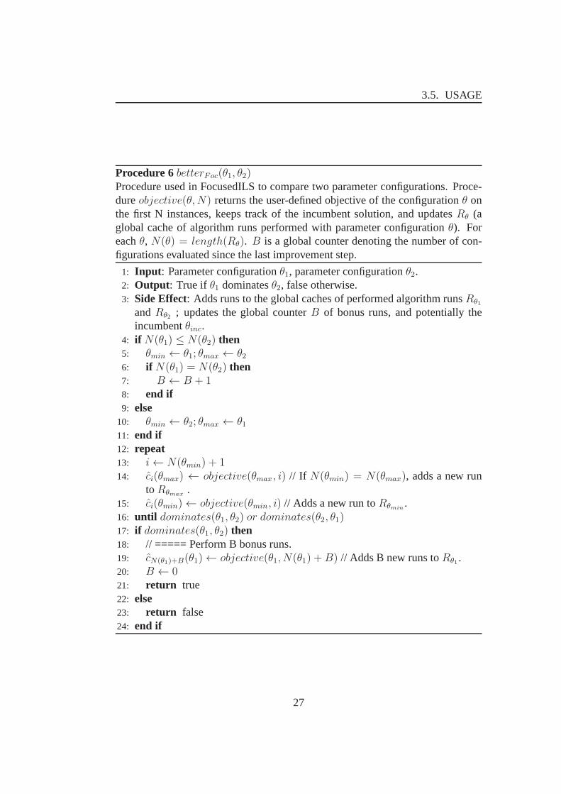
Procedure 6betterFoc(θ1, θ2)Procedure used in FocusedILS to compare two parameter configurations. Proce-dureobjective(θ,N) returns the user-defined objective of the configurationθ onthe first N instances, keeps track of the incumbent solution,and updatesRθ (aglobal cache of algorithm runs performed with parameter configurationθ). Foreachθ, N(θ) = length(Rθ). B is a global counter denoting the number of con-figurations evaluated since the last improvement step.
1: Input : Parameter configurationθ1, parameter configurationθ2.2: Output : True if θ1 dominatesθ2, false otherwise.3: Side Effect: Adds runs to the global caches of performed algorithm runsRθ1
andRθ2 ; updates the global counterB of bonus runs, and potentially theincumbentθinc.
4: if N(θ1) ≤ N(θ2) then5: θmin ← θ1; θmax ← θ26: if N(θ1) = N(θ2) then7: B ← B + 18: end if9: else
10: θmin ← θ2; θmax ← θ111: end if12: repeat13: i← N(θmin) + 114: ci(θmax) ← objective(θmax, i) // If N(θmin) = N(θmax), adds a new run
toRθmax.
15: ci(θmin)← objective(θmin, i) // Adds a new run toRθmin.
16: until dominates(θ1, θ2) or dominates(θ2, θ1)17: if dominates(θ1, θ2) then18: // ===== Perform B bonus runs.19: cN(θ1)+B(θ1)← objective(θ1, N(θ1) +B) // Adds B new runs toRθ1 .20: B ← 021: return true22: else23: return false24: end if
27

CHAPTER 3. PARAMILS
• maxEvalsThe number of algorithm executions after which the optimizationis terminated.
• maxIts The number of ILS iterations after which the optimization istermi-nated.
• approachUse basic for BasicILS, focused for FocusedILS, and random forrandom search.
• N For BasicILS, N is the number of runs to perform to evaluate each param-eter configuration. For FocusedILS, it is the maximal numberof runs toperform to evaluate a parameter configuration.
• userunlog If this parameter is 1 or true, another file ending in -runlog willbe placed in the output directory. This file will contain the configurationsand results for every algorithm run performed by ParamILS. There are alsoseveral internal parameters that control the heuristics inParamILS.
3.5.2 Tuning-scenario file
Tuning-scenario files such as this define a tuning scenario completely, and alsocontain some information about where ParamILS should writeits results, etc.They can contain the following information:
• algo An algorithm executable or a call to a wrapper script around an algo-rithm that conforms with the input/output format of ParamILS.
• execdir Directory to execute〈algo〉 from: ’cd 〈execdir〉; 〈algo〉’
• deterministic Set to 0 for randomized algorithms, 1 for deterministic
• run obj A scalar quantifying how ’good’ a single algorithm execution is,such as its required runtime. Implemented examples for thisinclude run-time, runlength, approx (approximation quality, i.e., 1-(optimal quality di-vided by found quality)), speedup (speedup over a referenceruntime for thisinstance - note that for this option the reference needs to bedefined in theinstance seed file as covered in Section 6). Additional objectives for sin-gle algorithm executions can be defined by modifying function single runobjective in file algospecifics.rb.
• overall obj While run obj defines the objective function for a single algo-rithm run, overall obj defines how those single objectives are combined toreach a single scalar value to compare two parameter configurations. Imple-mented examples include mean, median, q90 (the 90% quantile), adj mean
28

3.5. USAGE
(a version of the mean accounting for unsuccessful runs: total runtime di-vided by number of succesful runs), mean1000 (another version of the meanaccounting for unsuccessful runs: (total runtime of successful runs + 1000xruntime of unsuccessful runs) divided by number of runs - this effectivelymaximizes the number of successful runs, breaking ties by the runtime ofsuccessful runs), and geomean (geometric mean, primarily used in combi-nation with runobj = speedup. The empirical statistic of the cost distri-bution (across multiple instances and seeds) to be minimized, such as themean (of the single run objectives).
• cutoff time The time after which a single algorithm execution will be termi-nated unsuccesfully. This is an important parameter: if choosen too high,lots of time will be wasted with unsuccessful runs. If chosentoo low theoptimization is biased to perform well on easy instances only.
• cutoff length The run length after which a single algorithm execution willbe terminated unsuccessfully. This length can, e.g. be defined in flips for anSLS algorithm or decisions for a tree search.
• tunerTimeout The timeout of the tuner. Validation of the final best foundparameter configuration starts after the timeout.
• paramfile Specifies the file with the parameters of the algorithms.
• outdir Specifies the directory ParamILS should write its results to.
• instancefile Specifies the file with a list of training instances.
• test instance file Specifies the file with a list of test instances.
• instanceseedfile Specifies the file with a list of training instance/seed pairs- this and instance file are mutually exclusive.
• test instance seed fileSpecifies the file with a list of training instance/seedpairs - this and test instance file are mutually exclusive.
29

30

Part II
CONTRIBUTIONS
31


Chapter 4
Determine ParamILS Parameters
The experiments in this Section will clarify which are the most suitable ParamILSparameters for MathSAT. The most important ParamILS parameters are:
• approach the strategy that ParamILS uses to find the optimized configura-tions for ParamILS. We can set theapproachparameter asBasic, Focused,andRandomsearch. Because theBasic, andFocusedsearch are better thantheRandomsearch in all experiments of [2], therefore in this thesis weonlycheck whetherBasicor Focusedis the fittest one for MathSAT.
• deterministic the way ParamILS evaluates the target algorithm (MathSAT,in this case). Ifdeterministicis set to 1 (DAE), then ParamILS will onlyevaluate a single〈configuration, instance〉 pair once (with the seed of -1for the target algorithm, since the seed is not used by a deterministic targetalgorithm). Otherwise, thedeterministicparameter is set to 0 (RAE), thena 〈configuration, instance〉 pair will be evaluated several times, each with adifferent seed. This is in order to obtain a more representative picture of thealgorithm’s expected performance on that instance.
• cutoff-time the time after which a single algorithm execution will be termi-nated unsuccessfully. This is an important parameter because: if it is chosentoo high, lots of time will be wasted with unsuccessful runs.If it is chosentoo low the optimization is biased to perform well on easy instances only.
• tunerTimeout the timeout of the tuner (ParamILS). The validation of thefinal best found parameter configuration starts after this timeout.
• numRun the random seed for ParamILS.
33
CHAPTER 4. DETERMINE PARAMILS PARAMETERS
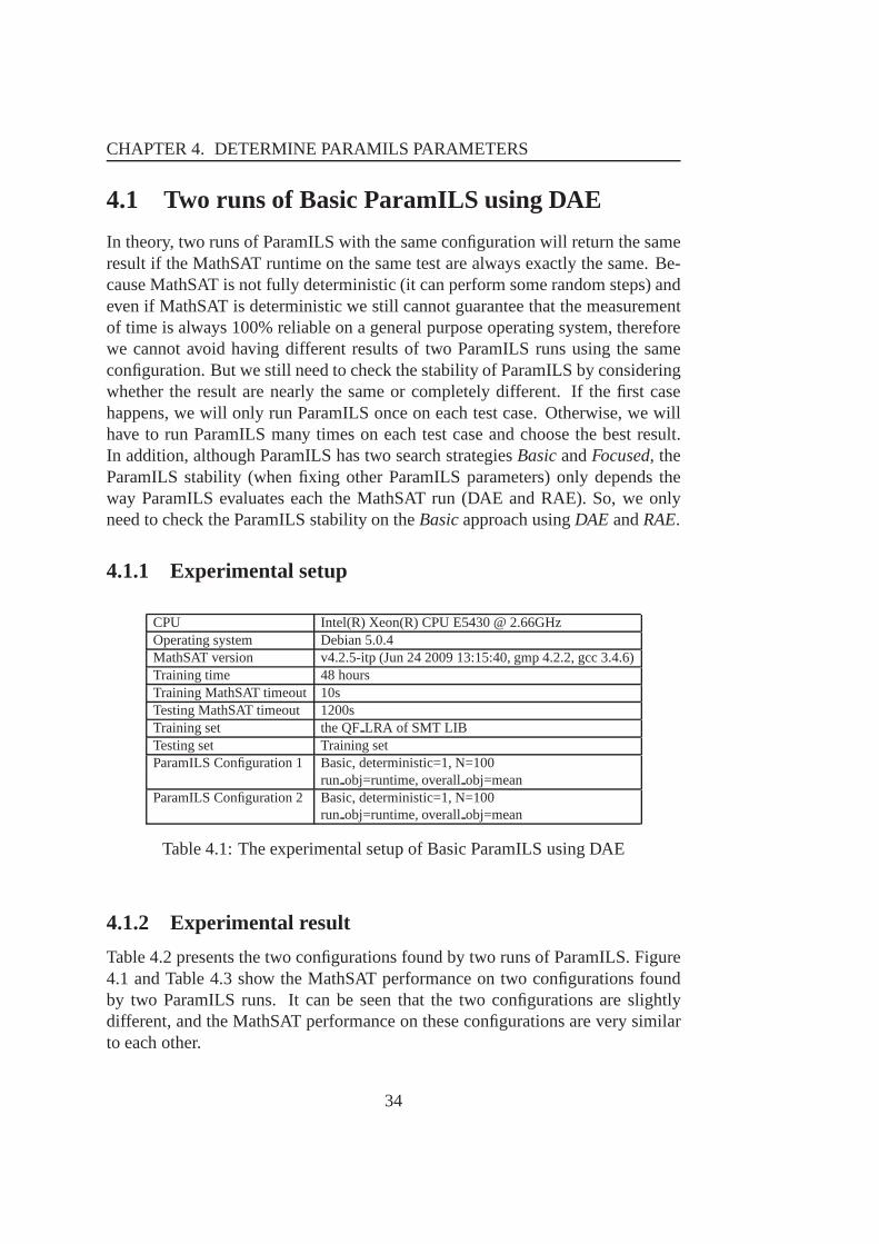
4.1 Two runs of Basic ParamILS using DAE
In theory, two runs of ParamILS with the same configuration will return the sameresult if the MathSAT runtime on the same test are always exactly the same. Be-cause MathSAT is not fully deterministic (it can perform some random steps) andeven if MathSAT is deterministic we still cannot guarantee that the measurementof time is always 100% reliable on a general purpose operating system, thereforewe cannot avoid having different results of two ParamILS runs using the sameconfiguration. But we still need to check the stability of ParamILS by consideringwhether the result are nearly the same or completely different. If the first casehappens, we will only run ParamILS once on each test case. Otherwise, we willhave to run ParamILS many times on each test case and choose the best result.In addition, although ParamILS has two search strategiesBasicandFocused, theParamILS stability (when fixing other ParamILS parameters)only depends theway ParamILS evaluates each the MathSAT run (DAE and RAE). So, we onlyneed to check the ParamILS stability on theBasicapproach usingDAE andRAE.
4.1.1 Experimental setup
CPU Intel(R) Xeon(R) CPU E5430 @ 2.66GHzOperating system Debian 5.0.4MathSAT version v4.2.5-itp (Jun 24 2009 13:15:40, gmp 4.2.2, gcc 3.4.6)Training time 48 hoursTraining MathSAT timeout 10sTesting MathSAT timeout 1200sTraining set the QFLRA of SMT LIBTesting set Training setParamILS Configuration 1 Basic, deterministic=1, N=100
run obj=runtime, overallobj=meanParamILS Configuration 2 Basic, deterministic=1, N=100
run obj=runtime, overallobj=mean
Table 4.1: The experimental setup of Basic ParamILS using DAE
4.1.2 Experimental result
Table 4.2 presents the two configurations found by two runs ofParamILS. Figure4.1 and Table 4.3 show the MathSAT performance on two configurations foundby two ParamILS runs. It can be seen that the two configurations are slightlydifferent, and the MathSAT performance on these configurations are very similarto each other.
34

4.1. TWO RUNS OF BASIC PARAMILS USING DAE
0.001
0.01
0.1
1
10
100
1000
10000
0.001 0.01 0.1 1 10 100 1000 10000
Def
ault
Optimized
Performance comparison
satisfiableunsatisfiableerror/timeout
(a) The first run
0.001
0.01
0.1
1
10
100
1000
10000
0.001 0.01 0.1 1 10 100 1000 10000
Def
ault
Optimized
Performance comparison
satisfiableunsatisfiableerror/timeout
(b) The second run
Figure 4.1: Performance comparison of two runs of Basic ParamILS with deter-ministic=1
35

CHAPTER 4. DETERMINE PARAMILS PARAMETERS
Configuration Default Basic DAE Basic DAEParameteraep yes yes yesdeduction 2 2 2dual rail off off offdyn ack no no yesdyn ack limit 0 0 0dyn ack threshold 1 1 50expensiveccmin yes no yesfrequentreducedb no no yesghostfilter no yes yesibliwi no yes yesimpl expl threshold 0 0 0mixed cs yes no nopermanenttheory lemmas yes yes yespure literal filter no yes yesrandomdecisions no no norestarts normal adaptive adaptivesl 2 2 2split eq no no notcomb off off acktoplevelprop 1 0 0tsolver euf la la euf la
Table 4.2: Experimental result of Basic ParamILS using DAE
Tests solved (Optimized/Default) 501/496Mean runtime(not include TIMEOUT tests) 30.639/29.202Optimized compared with Default ResultBetter runtime tests/The total number of tests 265/543Equal runtime tests/The total number of tests 92/543Worse runtime tests/The total number of tests 186/543
(a) The first run
Tests solved (Optimized/Default) 501/496Mean runtime(not include TIMEOUT tests) 25.978/29.999Optimized compared with Default ResultBetter runtime tests/The number of tests 255/543Equal runtime tests/The number of tests 105/543Worse runtime tests/The number of tests 183/543
(b) The second run
Table 4.3: Experimental result of Basic ParamILS using DAE
36

4.2. TWO RUNS OF BASIC PARAMILS USING RAE
4.2 Two runs of Basic ParamILS using RAE
The experiments in this section accompanied with the experiments in the previoussection are used to check the stability of ParamILS by considering whether theresults of two ParamILS runs are nearly the same or completely different. If thefirst case happens, we will only run ParamILS once on each testcase. Otherwise,we will have to run ParamILS many times on each test case and choose the bestresult.
4.2.1 Experimental setup
CPU Intel(R) Xeon(R) CPU E5430 @ 2.66GHzOperating system Debian 5.0.4MathSAT version v4.2.5-itp (Jun 24 2009 13:15:40, gmp 4.2.2, gcc 3.4.6)Training time 48 hoursTraining MathSAT timeout 10sTesting MathSAT timeout 1200sTraining set the QFLRA of SMT LIBTesting set Training setParamILS Configuration 1 Basic, deterministic=0, N=100
run obj=runtime, overallobj=meanParamILS Configuration 2 Basic, deterministic=0, N=100
run obj=runtime, overallobj=mean
Table 4.4: Experimental setup of two runs of Basic ParamILS using RAE
4.2.2 Experimental result
Table 4.5 presents two configurations found by two ParamILS runs. Figure 4.2and Table 4.6 show the MathSAT performance on two configurations found by twoParamILS runs. It can be seen that the two configurations are slightly different,and the MathSAT performance on these configurations are verysimilar to eachother.
37

CHAPTER 4. DETERMINE PARAMILS PARAMETERS
0.001
0.01
0.1
1
10
100
1000
10000
0.001 0.01 0.1 1 10 100 1000 10000
Def
ault
Optimized
Performance comparison
satisfiableunsatisfiableerror/timeout
(a) The first run
0.001
0.01
0.1
1
10
100
1000
10000
0.001 0.01 0.1 1 10 100 1000 10000
Def
ault
Optimized
Performance comparison
satisfiableunsatisfiableerror/timeout
(b) The second run
Figure 4.2: Performance comparison of Two runs of Basic ParamILS using RAE
38

4.2. TWO RUNS OF BASIC PARAMILS USING RAE
Configuration Default Basic RAE Basic RAEParameteraep yes no nodeduction 2 2 2dual rail off off offdyn ack no no nodyn ack limit 0 0 0dyn ack threshold 1 1 1expensiveccmin yes yes yesfrequentreducedb no no noghostfilter no yes noibliwi no yes yesimpl expl threshold 0 0 0mixed cs yes yes yespermanenttheory lemmas yes yes yespure literal filter no yes norandomdecisions no yes norestarts normal normal adaptivesl 2 2 2split eq no yes yestcomb off off offtoplevelprop 1 0 1tsolver euf la la la
Table 4.5: Experimental result of two runs of Basic ParamILSusing RAE
Tests solved (Optimized/Default) 524/496Mean runtime(not include TIMEOUT tests) 20.547/29.211Optimized compared with Default ResultBetter runtime tests/The number of tests 155/543Equal runtime tests/The number of tests 36/543Worse runtime tests/The number of tests 352/543
(a) The first run
Tests solved (Optimized/Default) 523/496Mean runtime(not include TIMEOUT test) 18.321/28.163Optimized compared with Default ResultBetter runtime tests/The number of tests 158/543Equal runtime tests/The number of tests 55/543Worse runtime tests/The number of tests 330/543
(b) The second run
Table 4.6: Experimental result of two runs of Basic ParamILSusing RAE
39

CHAPTER 4. DETERMINE PARAMILS PARAMETERS
4.3 Summary of two Basic ParamILS runs using DAEand RAE
From the summary result in Table 4.7, it can be seen that the MathSAT perfor-mances of configurations found by the two ParamILS runs are almost the same.The difference seems not to justify the overhead of running ParamILS severaltimes. Therefore, from now on, we have decided to run ParamILS once on eachtest case.
Default Basic DAE 1 Basic DAE 2 Basic RAE 1 Basic RAE 2Tests solved 496 501 501 524 523Mean runtime 28.163 30.639 25.978 20.547 18.321
Table 4.7: The number of solved tests and mean runtime in second (not includeTIMEOUT tests) of configurations found by Basic ParamILS using DAE and RAE
40

4.4. BASIC PARAMILS USING DAE AND RAE
4.4 Basic ParamILS using DAE and RAE
The purpose of the experiments in this section is to check which algorithm evalu-ation (DAE or RAE) Basic ParamILS uses is better for MathSAT.
4.4.1 Experimental setup
CPU Intel(R) Xeon(R) CPU E5430 @ 2.66GHzOperating system Debian 5.0.4MathSAT version v4.2.5-itp (Jun 24 2009 13:15:40, gmp 4.2.2, gcc 3.4.6)Training time 48 hoursTraining MathSAT timeout 10sTesting MathSAT timeout 1200sTraining set the QFLRA of SMT LIBTesting set Training setParamILS Configuration 1 Basic, deterministic=1, N=100
run obj=runtime, overallobj=meanParamILS Configuration 2 Basic, deterministic=0, N=100
run obj=runtime, overallobj=mean
Table 4.8: Experimental setup of Basic ParamILS using DAE and RAE
4.4.2 Experimental result
Tests solved (Optimized/Default) 501/496Mean runtime(not include TIMEOUT tests) 30.639/29.202Optimized compared with Default ResultBetter runtime tests/The number of tests 265/543Equal runtime tests/The number of tests 92/543Worse runtime tests/The number of tests 186/543
(a) Deterministic
Tests solved (Optimized/Default) 524/496Mean runtime(not include TIMEOUT tests) 20.547/29.114Optimized compared with Default ResultBetter runtime tests/The number of tests 155/543Equal runtime tests/The number of tests 36/543Worse runtime tests/The number of tests 352/543
(b) Random
Table 4.9: Experimental result of Basic ParamILS using DAE and RAE
41

CHAPTER 4. DETERMINE PARAMILS PARAMETERS
0.001
0.01
0.1
1
10
100
1000
10000
0.001 0.01 0.1 1 10 100 1000 10000
Def
ault
Optimized
Performance comparison
satisfiableunsatisfiableerror/timeout
(a) Deterministic
0.001
0.01
0.1
1
10
100
1000
10000
0.001 0.01 0.1 1 10 100 1000 10000
Def
ault
Optimized
Performance comparison
satisfiableunsatisfiableerror/timeout
(b) Random
Figure 4.3: Performance comparison of Basic ParamILS usingDAE and RAE
42

4.4. BASIC PARAMILS USING DAE AND RAE
The experimental results in Table 4.9 and Figure 4.3 show that Basic ParamILSusing RAE is better in this case, although MathSAT is a deterministic algorithm.The main reason is that Basic ParamILS evaluates every configuration only oncewith the same number of MathSAT runs, and the MathSAT run timeof the sameinstance on general purpose operating systems can vary in different runs. There-fore, RAE is more robust than DAE in the case of Basic ParamILSbecause RAEevaluates a single〈configuration, instance〉 pair many times, each with a differentseed (this helps to obtain a more representative picture of the algorithm’s expectedperformance on that instance).
43

CHAPTER 4. DETERMINE PARAMILS PARAMETERS
4.5 Focused ParamILS with DAE and RAE
The purpose of the experiments in this section is to check which algorithm evalu-ation (DAE or RAE) Focused ParamILS uses is better for MathSAT.
4.5.1 Experimental setup
CPU Intel(R) Xeon(R) CPU E5430 @ 2.66GHzOperating system Debian 5.0.4MathSAT version v4.2.5-itp (Jun 24 2009 13:15:40, gmp 4.2.2, gcc 3.4.6)Training time 48 hoursTraining MathSAT timeout 10sTesting MathSAT timeout 1200sTraining set the QFLRA of SMT LIBTesting set Training setParamILS Configuration 1 Focused, deterministic=1, N=543
run obj=runtime, overallobj=meanParamILS Configuration 2 Focused, deterministic=0, N=543
run obj=runtime, overallobj=mean
Table 4.10: The experimental setup of Focused ParamILS withdeterministic andrandom
4.5.2 Experimental result
Tests solved (Optimized/Default) 525/496Mean runtime(not include TIMEOUT tests) 24.367/28.903Optimized compared with Default ResultBetter runtime tests/The number of tests 148/543Equal runtime tests/The number of tests 40/543Worse runtime tests/The number of tests 355/543
(a) Deterministic
Tests solved (Optimized/Default) 523/496Mean runtime(not include TIMEOUT test) 18.150/28.593Optimized compared with Default ResultBetter runtime tests/The number of tests 165/543Equal runtime tests/The number of tests 56/543Worse runtime tests/The number of tests 322/543
(b) Random
Table 4.11: Experimental result of Focused ParamILS using DAE and RAE
44

4.5. FOCUSED PARAMILS WITH DAE AND RAE
0.001
0.01
0.1
1
10
100
1000
10000
0.001 0.01 0.1 1 10 100 1000 10000
Def
ault
Optimized
Performance comparison
satisfiableunsatisfiableerror/timeout
(a) Deterministic
0.001
0.01
0.1
1
10
100
1000
10000
0.001 0.01 0.1 1 10 100 1000 10000
Def
ault
Optimized
Performance comparison
satisfiableunsatisfiableerror/timeout
(b) Random
Figure 4.4: Performance comparison of Focused ParamILS using DAE and RAE
45

CHAPTER 4. DETERMINE PARAMILS PARAMETERS
The experimental results in Table 4.11 and Figure 4.4 show that FocusedParamILS using DAE is better. This is because although usingDAE, a Math-SAT run is evaluated only once, Focused ParamILS evaluates each configurationmany times, each with a different number of MathSAT runs. In other words, eval-uating a MathSAT run once still guarantees the configurationevaluation is preciseby evaluating that configuration many times. Besides, DAE saves a lot of timewhen evaluating a MathSAT run compared with RAE, and this makes FocusedParamILS evaluate a configuration more precisely by testingthat configuration ona large number of instances.
46

4.6. SUMMARY OF BASIC AND FOCUSED PARAMILS USING DAE ANDRAE
4.6 Summary of Basic and Focused ParamILS us-ing DAE and RAE
From the results in Table 4.12, it can be seen that Focused ParamILS is morestable than Basic ParamILS, and Focused ParamILS using DAE provides us withthe best performance. Therefore, Focused ParamILS using DAE is chosen forrunning on other experiments in this thesis.
Default Basic DAE Basic RAE Focused DAE Focused RAETests solved 496 501 524 525 523
Table 4.12: The number of tests solved (on 543 tests) of configurations found byBasic and Focused ParamILS using DAE and RAE
47

CHAPTER 4. DETERMINE PARAMILS PARAMETERS
4.7 RAE Basic ParamILS with different MathSATtimeouts
In order to choose the suitable MathSAT timeout (cutofftime), we base on thepercentage of tests solved by the default (or smt-comp) configuration using thatMathSAT timeout. The experiments in this section and the next section are usedto check whether ParamILS configured with the MathSAT timeouts in which thedefault configuration solves similar percentage of tests will have similar results.
4.7.1 Experimental setup
CPU Intel(R) Xeon(R) CPU E5430 @ 2.66GHzOperating system Debian 5.0.4MathSAT version v4.2.5-itp (Jun 24 2009 13:15:40, gmp 4.2.2, gcc 3.4.6)Training time 48 hoursTesting MathSAT timeout 1200sTraining set the QFLRA of SMT LIBTesting set Training setParamILS Configuration Basic, deterministic=0, N=100
run obj=runtime, overallobj=meanTraining MathSAT timeout 5s, 10s, 20s, 40s, 60s
Table 4.13: The experimental setup of Basic ParamILS with different MathSATtimeouts
MathSAT timeout 5s 10s 20s 40s 60sPercentage of tests solved 79.7% 82.5% 85.6% 88.8% 90.4%by the default configuration
Table 4.14: The percentage of tests solved when running MathSAT with differenttimeouts on the training set
4.7.2 Experimental result
From the results in Table 4.15 and Figure 4.5, except for timeout=5s, other Math-SAT timeouts have similar performance because the target algorithm MathSAT(using the default configuration) configured with these training timeouts solve ap-proximately the same percentage of instances in the training set.
48

4.7. RAE BASIC PARAMILS WITH DIFFERENT MATHSAT TIMEOUTS
0.001
0.01
0.1
1
10
100
1000
10000
0.001 0.01 0.1 1 10 100 1000 10000
Def
ault
Optimized
Performance comparison
satisfiableunsatisfiableerror/timeout
(a) training MathSAT timeout=5s
0.001
0.01
0.1
1
10
100
1000
10000
0.001 0.01 0.1 1 10 100 1000 10000
Def
ault
Optimized
Performance comparison
satisfiableunsatisfiableerror/timeout
(b) training MathSAT timeout=10s
Figure 4.5: Performance comparison of Basic ParamILS with different trainingMathSAT timeouts
49
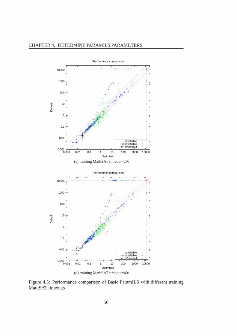
CHAPTER 4. DETERMINE PARAMILS PARAMETERS
0.001
0.01
0.1
1
10
100
1000
10000
0.001 0.01 0.1 1 10 100 1000 10000
Def
ault
Optimized
Performance comparison
satisfiableunsatisfiableerror/timeout
(c) training MathSAT timeout=20s
0.001
0.01
0.1
1
10
100
1000
10000
0.001 0.01 0.1 1 10 100 1000 10000
Def
ault
Optimized
Performance comparison
satisfiableunsatisfiableerror/timeout
(d) training MathSAT timeout=40s
Figure 4.5: Performance comparison of Basic ParamILS with different trainingMathSAT timeouts
50

4.7. RAE BASIC PARAMILS WITH DIFFERENT MATHSAT TIMEOUTS
0.001
0.01
0.1
1
10
100
1000
10000
0.001 0.01 0.1 1 10 100 1000 10000
Def
ault
Optimized
Performance comparison
satisfiableunsatisfiableerror/timeout
(e) training MathSAT timeout=60s
Figure 4.5: Performance comparison of Basic ParamILS with different trainingMathSAT timeouts
51

CHAPTER 4. DETERMINE PARAMILS PARAMETERS
Tests solved (Optimized/Default) 500/496Mean runtime(not include TIMEOUT tests) 29.194/28.274Optimized compared with Default ResultBetter runtime tests/The number of tests 280/543Equal runtime tests/The number of tests 97/543Worse runtime tests/The number of tests 166/543
(a) training MathSAT timeout=5s
Tests solved (Optimized/Default) 524/496Mean runtime(not include TIMEOUT tests) 20.547/29.211Optimized compared with Default ResultBetter runtime tests/The number of tests 155/543Equal runtime tests/The number of tests 36/543Worse runtime tests/The number of tests 352/543
(b) training MathSAT timeout=10s
Tests solved (Optimized/Default) 520/496Mean runtime(not include TIMEOUT tests) 23.137/30.939Optimized compared with Default ResultBetter runtime tests/The number of tests 123/543Equal runtime tests/The number of tests 34/543Worse runtime tests/The number of tests 386/543
(c) training MathSAT timeout=20s
Tests solved (Optimized/Default) 521/496Mean runtime(not include TIMEOUT tests) 22.308/31.188Optimized compared with Default ResultBetter runtime tests/The number of tests 120/543Equal runtime tests/The number of tests 49/543Worse runtime tests/The number of tests 374/543
(d) training MathSAT timeout=40s
Tests solved (Optimized/Default) 521/495Mean runtime(not include TIMEOUT tests) 21.072/30.121Optimized compared with Default ResultBetter runtime tests/The number of tests 132/543Equal runtime tests/The number of tests 47/543Worse runtime tests/The number of tests 364/543
(e) training MathSAT timeout=60s
Table 4.15: Experimental result of RAE Basic ParamILS with different trainingMathSAT timeouts
52

4.8. DAE FOCUSED PARAMILS WITH DIFFERENT TRAINING MATHSATTIMEOUTS
4.8 DAE Focused ParamILS with different trainingMathSAT timeouts
In order to choose the suitable MathSAT timeout (cuttofftime), we base on thepercentage of tests solved by the default (or smt-comp) configuration using thatMathSAT timeout. The experiments in this section and the previous section areused to check whether ParamILS configured with the MathSAT timeouts in whichthe default configuration solves similar percentage of tests will have similar re-sults.
4.8.1 Experimental setup
CPU Intel(R) Xeon(R) CPU E5430 @ 2.66GHzOperating system Debian 5.0.4MathSAT version v4.2.5-itp (Jun 24 2009 13:15:40, gmp 4.2.2, gcc 3.4.6)Training time 48 hoursTesting MathSAT timeout 1200sTraining set the QFLRA of SMT LIBTesting set Training setParamILS Configuration Focused, deterministic=1, N=543
run obj=runtime, overallobj=meanTraining MathSAT timeout 5s, 10s, 20s, 40s, 60s
Table 4.16: The experimental setup of DAE Focused ParamILS with differenttimeouts
MathSAT timeout 5s 10s 20s 40s 60sPercentage os tests solved 79.7% 82.5% 85.6% 88.8% 90.4%by the default configuration
Table 4.17: The percentage of tests solved and mean runtime when running Math-SAT with different MathSAT timeouts on the training set
4.8.2 Experimental result
From the results in Table 4.18 and Figure 4.6, except for training MathSAT time-out=5s, other training MathSAT timeouts have similar performance because thetarget algorithm MathSAT (using the default configuration)configured with thesetraining MathSAT timeouts solve approximately the same percentage of instancesin the training set.
53

CHAPTER 4. DETERMINE PARAMILS PARAMETERS
0.001
0.01
0.1
1
10
100
1000
10000
0.001 0.01 0.1 1 10 100 1000 10000
Def
ault
Optimized
Performance comparison
satisfiableunsatisfiableerror/timeout
(a) timeout=5s
0.001
0.01
0.1
1
10
100
1000
10000
0.001 0.01 0.1 1 10 100 1000 10000
Def
ault
Optimized
Performance comparison
satisfiableunsatisfiableerror/timeout
(b) timeout=10s
Figure 4.6: Performance comparison of DAE Focused ParamILSwith differentMathSAT timeouts
54

4.8. DAE FOCUSED PARAMILS WITH DIFFERENT TRAINING MATHSATTIMEOUTS
0.001
0.01
0.1
1
10
100
1000
10000
0.001 0.01 0.1 1 10 100 1000 10000
Def
ault
Optimized
Performance comparison
satisfiableunsatisfiableerror/timeout
(c) timeout=20s
0.001
0.01
0.1
1
10
100
1000
10000
0.001 0.01 0.1 1 10 100 1000 10000
Def
ault
Optimized
Performance comparison
satisfiableunsatisfiableerror/timeout
(d) timeout=40s
Figure 4.6: Performance comparison of DAE Focused ParamILSwith differentMathSAT timeouts
55
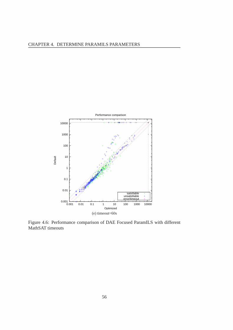
CHAPTER 4. DETERMINE PARAMILS PARAMETERS
0.001
0.01
0.1
1
10
100
1000
10000
0.001 0.01 0.1 1 10 100 1000 10000
Def
ault
Optimized
Performance comparison
satisfiableunsatisfiableerror/timeout
(e) timeout=60s
Figure 4.6: Performance comparison of DAE Focused ParamILSwith differentMathSAT timeouts
56

4.8. DAE FOCUSED PARAMILS WITH DIFFERENT TRAINING MATHSATTIMEOUTS
Tests solved (Optimized/Default) 496/495Mean runtime(not include TIMEOUT tests) 28.651s/28.633sOptimized compared with Default ResultBetter runtime tests/The number of tests 275/543Equal runtime tests/The number of tests 102/543Worse runtime tests/The number of tests 166/543
(a) timeout=5s
Tests solved (Optimized/Default) 523/495Mean runtime(not include TIMEOUT tests) 19.407s/28.953sOptimized compared with Default ResultBetter runtime tests/The number of tests 182/543Equal runtime tests/The number of tests 50/543Worse runtime tests/The number of tests 311/543
(b) timeout=10s
Tests solved (Optimized/Default) 519/495Mean runtime(not include TIMEOUT tests) 21.957s/30.743sOptimized compared with Default ResultBetter runtime tests/The number of tests 129/543Equal runtime tests/The number of tests 56/543Worse runtime tests/The number of tests 358/543
(c) timeout=20s
Tests solved (Optimized/Default) 520/496Mean runtime(not include TIMEOUT tests) 19.954s/30.789sOptimized compared with Default ResultBetter runtime tests/The number of tests 155/543Equal runtime tests/The number of tests 59/543Worse runtime tests/The number of tests 329/543
(d) timeout=40s
Tests solved (Optimized/Default) 522/496Mean runtime(not include TIMEOUT tests) 18.814s/30.496sOptimized compared with Default ResultBetter runtime tests/The number of tests 166/543Equal runtime tests/The number of tests 50/543Worse runtime tests/The number of tests 327/543
(e) timeout=60s
Table 4.18: Performance comparison of DAE Focused ParamILSwith differenttraining MathSAT timeouts
57

CHAPTER 4. DETERMINE PARAMILS PARAMETERS
4.9 DAE Focused ParamILS with different trainingtimes
ParamILS configured with the MathSAT timeout of 60s converges within 48 hours(by considering the ParamILS log file). The experiments in this section are usedto check whether we can get the over-training situation by expanding the trainingtime to 72 hours.
4.9.1 Experimental setup
CPU Intel(R) Xeon(R) CPU E5430 @ 2.66GHzOperating system Debian 5.0.4MathSAT version v4.2.5-itp (Jun 24 2009 13:15:40, gmp 4.2.2, gcc 3.4.6)Training MathSAT timeout 60sTesting MathSAT timeout 1200sTraining set the QFLRA of SMT LIBTesting set Training setParamILS Configuration Focused, deterministic=1, N=543
run obj=runtime, overallobj=meanTraining time 1 48 hoursTraining time 2 72 hours
Table 4.19: The experimental setup of DAE Focused ParamILS with differenttraining times
4.9.2 Experimental result
The results in Table 4.20 and Figure 4.7 show that we can get the over-trainingsituation. Therefore, if the MathSAT timeout is less than orequal to 60s, weshould not train ParamILS more than 48 hours.
58

4.9. DAE FOCUSED PARAMILS WITH DIFFERENT TRAINING TIMES
0.001
0.01
0.1
1
10
100
1000
10000
0.001 0.01 0.1 1 10 100 1000 10000
Def
ault
Optimized
Performance comparison
satisfiableunsatisfiableerror/timeout
(a) Training time = 48hours
0.001
0.01
0.1
1
10
100
1000
10000
0.001 0.01 0.1 1 10 100 1000 10000
Def
ault
Optimized
Performance comparison
satisfiableunsatisfiableerror/timeout
(b) Training time = 72hours
Figure 4.7: Performance comparison of Focused ParamILS, deterministic=1 withdifferent training times
59

CHAPTER 4. DETERMINE PARAMILS PARAMETERS
Tests solved (Optimized/Default) 522/496Mean runtime(not include TIMEOUT tests) 18.814s/30.496sOptimized compared with Default ResultBetter runtime tests/The number of tests 166/543Equal runtime tests/The number of tests 50/543Worse runtime tests/The number of tests 327/543
(a) Training time = 48hours
Tests solved (Optimized/Default) 519/495Mean runtime(not include TIMEOUT tests) 19.442s/27.850sOptimized compared with Default ResultBetter runtime tests/The number of tests 167/543Equal runtime tests/The number of tests 51/543Worse runtime tests/The number of tests 325/543
(b) Training time = 72 hours
Table 4.20: Performance comparison of DAE Focused ParamILSwith differenttraining times
60

4.10. DAE FOCUSED PARAMILS WITH DIFFERENT NUMRUNS
4.10 DAE Focused ParamILS with different num-Runs
Because the ParamILS random behaviour depends on a random seed, numRun,therefore we need to check whether ParamILS performances with different ran-dom seeds are completely different or similar to each other.The experiments inthis section are used to verify this property.
4.10.1 Experimental setup
CPU Intel(R) Xeon(R) CPU E5430 @ 2.66GHzOperating system Debian 5.0.4MathSAT version v4.2.5-itp (Jun 24 2009 13:15:40, gmp 4.2.2, gcc 3.4.6)Tunning time 48 hoursTraining MathSAT timeout 10sTesting MathSAT timeout 1200sTraining set the QFLRA of SMT LIBTesting set Training setParamILS Configuration Focused, deterministic=1, N=543
run obj=runtime, overallobj=meannumRun 1, 2, 3
Table 4.21: Experimental setup of DAE Focused ParamILS withdifferent num-Runs
4.10.2 Experimental result
The results in Table 4.22 and Figure 4.8 show that ParamILS has nearly the sameperformance on different numRuns. Hence, we fix the numRun parameter forother experiments in this thesis.
61

CHAPTER 4. DETERMINE PARAMILS PARAMETERS
Tests solved (Optimized/Default) 523/496Mean runtime(not include TIMEOUT tests) 22.373s/30.867sOptimized compared with Default ResultBetter runtime tests/The number of tests 180/543Equal runtime tests/The number of tests 48/543Worse runtime tests/The number of tests 315/543
(a) numRun 1
Tests solved (Optimized/Default) 523/496Mean runtime(not include TIMEOUT tests) 18.165s/28.200sOptimized compared with Default ResultBetter runtime tests/The number of tests 186/543Equal runtime tests/The number of tests 52/543Worse runtime tests/The number of tests 305/543
(b) numRun 2
Tests solved (Optimized/Default) 523/495Mean runtime(not include TIMEOUT tests) 19.407s/28.953sOptimized compared with Default ResultBetter runtime tests/The number of tests 182/543Equal runtime tests/The number of tests 50/543Worse runtime tests/The number of tests 311/543
(c) numRun 3
Table 4.22: Performance comparison of DAE Focused ParamILSwith differentnumRuns
62

4.10. DAE FOCUSED PARAMILS WITH DIFFERENT NUMRUNS
0.001
0.01
0.1
1
10
100
1000
10000
0.001 0.01 0.1 1 10 100 1000 10000
Def
ault
Optimized
Performance comparison
satisfiableunsatisfiableerror/timeout
(a) numRun 1
0.001
0.01
0.1
1
10
100
1000
10000
0.001 0.01 0.1 1 10 100 1000 10000
Def
ault
Optimized
Performance comparison
satisfiableunsatisfiableerror/timeout
(b) numRun 2
Figure 4.8: Performance comparison of DAE Focused ParamILSwith differentnumRuns
63

CHAPTER 4. DETERMINE PARAMILS PARAMETERS
0.001
0.01
0.1
1
10
100
1000
10000
0.001 0.01 0.1 1 10 100 1000 10000
Def
ault
Optimized
Performance comparison
satisfiableunsatisfiableerror/timeout
(c) numRun 3
Figure 4.8: Performance comparison of DAE Focused ParamILSwith differentnumRuns
64

4.11. SUMMARY
4.11 Summary
From the experimental results in this section, we conclude thatFocused ParamILSusing DAEis the most suitable configuration of ParamILS for MathSAT. As for thetraining time,48 hoursis enough for the ParamILS convergence because we ex-perimented on theQF LRA, one of the most difficult theories in the set of theoriessupported by MathSAT, and observed that ParamILS convergedwithin 48 train-ing hourswith the MathSAT timeouts less than 60s. In order to choose suitableMathSAT timeouts when training, we run MathSAT with the default (or smtcomp)configuration on the training dataset in advance and choose the three MathSATtimeouts (all timeouts have value from 0 to 1200 with step of 5) which are lessthan 60 seconds and solve similar percentage of tests.
65

66

Chapter 5
Configuring MathSAT on FiveTheories on the SMT-COMPBenchmark
This section shows the results of using ParamILS to find the best possible config-urations for twelve theories implemented by MathSAT on the SMT-COMP 2009benchmark. The experiments in this section use the same dataset of SMT-COMP2009 for training and testing because we want to get the best possible MathSATconfigurations for the SMT-COMP 2009. In addition, MathSAT is under heavydevelopment, therefore these experiments help a lot in revealing MathSAT bugs.
The experiment setup for all tests in this chapter is summarised as follows:Based on the experimental results in Chapter 4, Focused ParamILS using DAE isthe best strategy for MathSAT. In addition, the training time of 48 hours is enoughfor MathSAT to converge with the MathSAT timeouts less than 60 seconds. Asfor choosing the training MathSAT timeouts, we run MathSAT with the smt-compconfiguration on the training dataset in advance and choose the three MathSATtimeouts (all timeouts have value from 0 to 1200 with step 5) which are less than60 seconds and solve similar percentage of tests.
Notice that the smt-comp configurations areadaptive, i.e. they can be changedaccording to different problem classes based on a statistics module in MathSAT.
Before moving to the next sections of experiments, we introduce briefly thefive theories [17] :
• QF IDL : Difference Logic over the integers. In essence, Boolean combi-nations of inequations of the form(x − y < b) where x and y are integervariables and b is an integer constant.
• QF LIA : Unquantified linear integer arithmetic. In essence, Boolean com-binations of inequations between linear polynomials over integer variables.
67

CHAPTER 5. CONFIGURING MATHSAT ON FIVE THEORIES ON THESMT-COMP BENCHMARK
These inequations are written in the form(a1.x1 + ... + an.xn ⊲⊳ a0), s.t.⊲⊳ ∈ {≤, <, 6=,=,≥, >}.
• QF LRA : Unquantified linear real arithmetic. In essence, Boolean combi-nations of inequations between linear polynomials over real variables.
• QF UFIDL : Difference Logic over the integers (in essence) but with unin-terpreted sort and function symbols (QFUF is described in chapter 6). Forexample:
UF : (f(x1) = f(x2)) ∧ ¬(f(x2) = f(x3))
IDL : (x1 − x3 < 1) ∧ (x3 − x1 < 1)
• QF UFLRA : Unquantified linear real arithmetic with uninterpreted sortand function symbols.
68

5.1. QFIDL WITH FOCUSED PARAMILS USING DAE
5.1 QF IDL with Focused ParamILS using DAE
5.1.1 Experimental setup
CPU Intel(R) Xeon(R) CPU E5430 @ 2.66GHzOperating system Debian 5.0.4MathSAT version v4.2.10-itp (May 12 2010 08:54:51, gmp 4.3.2, gcc 4.4.3)Training MathSAT timeout 1 35s (the smt-comp configuration solved 75.49% of tests)Training MathSAT timeout 2 40s (the smt-comp configuration solved 76.47% of tests)Training MathSAT timeout 3 45s (the smt-comp configuration solved 76.47% of tests)Testing MathSAT timeout 1200sTraining time 48 hoursTraining set the QFIDL of SMT-COMP 2009Testing set Training setParamILS Configuration Focused, deterministic=1, N=102
run obj=runtime, overallobj=mean
Table 5.1: The experimental setup of QFIDL with different training MathSATtimeouts
5.1.2 Training Result
Table 5.2 shows the default configuration and the optimized configurations foundby running ParamILS with different MathSAT timeouts. Thebold font is usedto show the difference between configurations. It can be seenthat for QFIDL,ghostfilter andincr solversshould be enabled, whilemixedcsandsplit eqshouldbe disabled. Besides, thedeductionlevel should be 2 instead of 0 as default andthestatic learning(sl) level should be 1 instead of 2 as default.
5.1.3 Testing Result
Table 5.3 and Figure 5.1 show the performance comparison between the opti-mized, default and adaptive smt-comp configurations. The optimized configu-rations solve14 tests, 12 tests, and 13 tests more compared with the adaptivesmt-comp configuration. Moreover, the winner on this theoryin the SMT compe-tition 2009 can solve only86 testsbut the best optimized configuration can solve96 tests(despite the fact that we are using the older version of MathSAT in thisexperiment, not the one in the SMT competition 2009). The result is a significantimprovement because the smt-comp configuration is anadaptiveconfiguration
69

CHAPTER 5. CONFIGURING MATHSAT ON FIVE THEORIES ON THESMT-COMP BENCHMARK
Configuration Default 35s 40s 45sParameteraep yes yes yes yesdeduction 2 0 0 0dual rail off off off offdyn ack no no no nodyn ack limit 0 0 0 0dyn ack threshold 1 1 1 1expensiveccmin yes yes no nofrequentreducedb no no no noghost filter no yes yes yesibliwi yes yes yes yesimpl expl threshold 0 1 1 0incr tsolvers no yes yes yesmixed cs yes no no nopermanenttheory lemmas yes yes no yespure literal filter no no no norandomdecisions no no no norestarts normal adaptive normal normalsl 2 1 1 1split eq yes no no notcomb off off off offtoplevelprop 1 2 1 1tsolver dl dl dl dl
Table 5.2: QFIDL configurations found by different training MathSAT timeouts
70

5.1. QFIDL WITH FOCUSED PARAMILS USING DAE
which is the combination of many a prior chosen configurations and changed ac-cording to different problem classes while the optimized configuration isfixed forall tests.
Tests solved (Optimized/Default/SMTCOMP) 96/81/82Mean runtime (not include TIMEOUT tests) 14.755s/25.069s/40.349sOptimized compared with Default ResultBetter runtime tests/The number of tests 63/102Equal runtime tests/The number of tests 21/102Worse runtime tests/The number of tests 18/102
(a) training MathSAT timeout = 35s
Tests solved (Optimized/Default/SMTCOMP) 94/81/82Mean runtime(not include TIMEOUT tests) 22.805s/25.069s/40.349sOptimized compared with Default ResultBetter runtime tests/The number of tests 54/102Equal runtime tests/The number of tests 30/102Worse runtime tests/The number of tests 18/102
(b) training MathSAT timeout = 40s
Tests solved (Optimized/Default/SMTCOMP) 95/81/82Mean runtime(not include TIMEOUT tests) 13.165s/25.069s/40.349sOptimized compared with Default ResultBetter runtime tests/The number of tests 58/102Equal runtime tests/The number of tests 28/102Worse runtime tests/The number of tests 16/102
(c) training MathSAT timeout = 45s
Table 5.3: Performance comparison of QFIDL configurations found by differenttraining MathSAT timeouts
71

CHAPTER 5. CONFIGURING MATHSAT ON FIVE THEORIES ON THESMT-COMP BENCHMARK
0.001
0.01
0.1
1
10
100
1000
10000
0.001 0.01 0.1 1 10 100 1000 10000
Def
ault
Optimized
Performance comparison
satisfiableunsatisfiableerror/timeout
(a) training MathSAT timeout = 35s
Figure 5.1: Performance comparison of QFIDL configurations found by differenttraining MathSAT timeouts
72

5.1. QFIDL WITH FOCUSED PARAMILS USING DAE
0.001
0.01
0.1
1
10
100
1000
10000
0.001 0.01 0.1 1 10 100 1000 10000
Def
ault
Optimized
Performance comparison
satisfiableunsatisfiableerror/timeout
(b) training MathSAT timeout = 40s
0.001
0.01
0.1
1
10
100
1000
10000
0.001 0.01 0.1 1 10 100 1000 10000
Def
ault
Optimized
Performance comparison
satisfiableunsatisfiableerror/timeout
(c) training MathSAT timeout = 45s
Figure 5.1: Performance comparison of QFIDL configurations found by differenttraining MathSAT timeouts (cont.)
73

CHAPTER 5. CONFIGURING MATHSAT ON FIVE THEORIES ON THESMT-COMP BENCHMARK
5.2 QF LIA with Focused ParamILS using DAE
5.2.1 Experimental setup
CPU Intel(R) Xeon(R) CPU E5430 @ 2.66GHzOperating system Debian 5.0.4MathSAT version v4.2.10-itp (May 12 2010 08:54:51, gmp 4.3.2, gcc 4.4.3)Training MathSAT timeout 1 50s (the smt-comp configuration solved 83.41% of tests)Training MathSAT timeout 2 55s (the smt-comp configuration solved 83.90% of tests)Training MathSAT timeout 3 60s (the smt-comp configuration solved 85.58% of tests)Testing MathSAT timeout 1200sTraining time 48 hoursTraining set the QFLIA of SMT-COMP 2009Testing set Training setParamILS Configuration Focused, deterministic=1, N=205
run obj=runtime, overallobj=mean
Table 5.4: The experimental setup of QFLIA with different training MathSATtimeouts
5.2.2 Training Result
Table 5.5 shows the default configuration and the optimized configurations foundby ParamILS. For this theory, ParamILS suggests thataep, pure literal filter, andsplit eqshould be disabled whileghostfilter, ibliwi , andrandomdecisionsshouldbe enabled. In addition, thestatic learninglevel (sl) should be 0 instead of 2 asdefault and using one theory solverla is better to solve this theory than using twotheorieseuf, and laas default.
5.2.3 Testing Result
Table 5.6 and Figure 5.2 show the performance comparison between the opti-mized, default and adaptive smt-comp configuration. In three optimized configu-rations, the optimized configuration found by the MathSAT timeout of 60 secondshas the mean runtimereduced by halfcompared with the mean runtime of theadaptivesmt-comp configuration.
74

5.2. QFLIA WITH FOCUSED PARAMILS USING DAE
Configuration Default 50s 55s 60sParameteraep yes no no nodeduction 2 2 2 2dual rail off off off offdyn ack no no no nodyn ack limit 0 0 0 0dyn ack threshold 1 1 1 1expensiveccmin yes no no yesfrequentreducedb no no yes yesghost filter no yes yes yesibliwi no yes yes yesimpl expl threshold 0 0 0 0incr tsolvers no yes yes yesmixed cs yes yes no nopermanenttheory lemmas yes yes yes nopure literal filter yes no no norandom decisions no yes yes yesrestarts normal normal quick quicksl 2 0 0 0split eq yes no no notcomb off off off offtoplevelprop 1 0 0 1tsolver euf laz laz laz laz
Table 5.5: QFLIA configurations found by different training MathSAT timeouts
75

CHAPTER 5. CONFIGURING MATHSAT ON FIVE THEORIES ON THESMT-COMP BENCHMARK
Tests solved (Optimized/Default/SMTCOMP) 201/201/202Mean runtime (not include TIMEOUT tests) 11.892s/15.495s/26.322sOptimized compared with Default ResultBetter runtime tests/The number of tests 165/205Equal runtime tests/The number of tests 12/205Worse runtime tests/The number of tests 28/205
(a) training MathSAT timeout = 50s
Tests solved (Optimized/Default/SMTCOMP) 201/201/202Mean runtime(not include TIMEOUT tests) 13.377s/15.495s/26.322sOptimized compared with Default ResultBetter runtime tests/The number of tests 165/205Equal runtime tests/The number of tests 8/205Worse runtime tests/The number of tests 32/205
(b) training MathSAT timeout = 55s
Tests solved (Optimized/Default/SMTCOMP) 202/201/202Mean runtime(not include TIMEOUT tests) 13.850s/15.495s/26.322sOptimized compared with Default ResultBetter runtime tests/The number of tests 164/202Equal runtime tests/The number of tests 9/202Worse runtime tests/The number of tests 32/202
(c) training MathSAT timeout = 60s
Table 5.6: Performance comparison of QFLIA configurations found by differenttraining MathSAT timeouts
76

5.2. QFLIA WITH FOCUSED PARAMILS USING DAE
0.001
0.01
0.1
1
10
100
1000
10000
0.001 0.01 0.1 1 10 100 1000 10000
Def
ault
Optimized
Performance comparison
satisfiableunsatisfiableerror/timeout
(a) training MathSAT timeout = 50s
Figure 5.2: Performance comparison of QFLIA configurations found by differenttraining MathSAT timeouts
77

CHAPTER 5. CONFIGURING MATHSAT ON FIVE THEORIES ON THESMT-COMP BENCHMARK
0.001
0.01
0.1
1
10
100
1000
10000
0.001 0.01 0.1 1 10 100 1000 10000
Def
ault
Optimized
Performance comparison
satisfiableunsatisfiableerror/timeout
(b) training MathSAT timeout = 55s
0.001
0.01
0.1
1
10
100
1000
10000
0.001 0.01 0.1 1 10 100 1000 10000
Def
ault
Optimized
Performance comparison
satisfiableunsatisfiableerror/timeout
(c) training MathSAT timeout = 60s
Figure 5.2: Performance comparison of QFLIA configurations found by differenttraining MathSAT timeouts (cont.)
78

5.3. QFLRA WITH FOCUSED PARAMILS USING DAE
5.3 QF LRA with Focused ParamILS using DAE
5.3.1 Experimental setup
CPU Intel(R) Xeon(R) CPU E5430 @ 2.66GHzOperating system Debian 5.0.4MathSAT version v4.2.10-itp (May 12 2010 08:54:51, gmp 4.3.2, gcc 4.4.3)Training MathSAT timeout 1 40s (the smt-comp configuration solved 85.64 % of tests)Training MathSAT timeout 2 45s (the smt-comp configuration solved 86.13% of tests)Training MathSAT timeout 3 50s (the smt-comp configuration solved 86.63% of tests)Testing MathSAT timeout 1200sTraining time 48 hoursTraining set the QFLRA of SMT-COMP 2009Testing set Training setParamILS Configuration Focused, deterministic=1, N=202
run obj=runtime, overallobj=mean
Table 5.7: The experimental setup of QFLRA with different training MathSATtimeouts
5.3.2 Training Result
Table 5.8 shows the default configuration and the optimized configurations foundby ParamILS. The main difference between the optimized configurations and thedefault configuration is thatpure literal filter is disabled (instead of being enabledas default) andsplit eq is enabled (instead of being disabled by default), and onlyone theoryla is used in the optimized configurations while the default configura-tion uses two theories solvereuf, and la.
5.3.3 Testing Result
Table 5.9 and Figure 5.3 show the performance comparison between the opti-mized, default and adaptive smt-comp configurations. It canbe seen that the firstoptimized configuration solve1 testmore compared with theadaptive smt-compconfiguration and the other two optimized configurations hasthe mean runtimereduced by a factor of around 1.5compared with theadaptive smt-compconfigu-ration. If compared with the default configuration, the three optimized configura-tions solve7, or 6 tests more.
79

CHAPTER 5. CONFIGURING MATHSAT ON FIVE THEORIES ON THESMT-COMP BENCHMARK
Configuration Default 40s 45s 50sParameteraep yes yes no nodeduction 2 2 2 2dual rail off off off offdyn ack no no no nodyn ack limit 0 0 0 0dyn ack threshold 1 1 1 1expensiveccmin yes yes yes nofrequentreducedb no yes no noghostfilter no no no yesibliwi no yes no noimpl expl threshold 0 0 0 0incr tsolvers no no no nomixed cs yes yes yes yespermanenttheory lemmas yes yes yes nopure literal filter yes no no norandomdecisions no yes no norestarts normal quick adaptive normalsl 2 2 2 1split eq no yes yes yestcomb off off off offtoplevelprop 1 1 1 1tsolver euf la la la la
Table 5.8: QFLRA configurations found by different training MathSAT timeouts
80

5.3. QFLRA WITH FOCUSED PARAMILS USING DAE
Tests solved (Optimized/Default/SMTCOMP) 184/177/183Mean runtime(not include TIMEOUT tests) 27.641s/35.057s/19.177sOptimized compared with Default ResultBetter runtime tests/The number of tests 68/202Equal runtime tests/The number of tests 37/202Worse runtime tests/The number of tests 97/202
(a) training MathSAT timeout = 40s
Tests solved (Optimized/Default/SMTCOMP) 183/177/183Mean runtime(not include TIMEOUT tests) 12.988s/35.057s/19.177sOptimized compared with Default ResultBetter runtime tests/The number of tests 76/202Equal runtime tests/The number of tests 33/202Worse runtime tests/The number of tests 93/202
(b) training MathSAT timeout = 45s
Tests solved (Optimized/Default/SMTCOMP) 183/177/183Mean runtime(not include TIMEOUT tests) 13.155s/35.057s/19.177sOptimized compared with Default ResultBetter runtime tests/The number of tests 78/202Equal runtime tests/The number of tests 32/202Worse runtime tests/The number of tests 92/202
(c) training MathSAT timeout = 50s
Table 5.9: Performance comparison of QFLRA configurations found by differenttraining MathSAT timeouts
81

CHAPTER 5. CONFIGURING MATHSAT ON FIVE THEORIES ON THESMT-COMP BENCHMARK
0.001
0.01
0.1
1
10
100
1000
10000
0.001 0.01 0.1 1 10 100 1000 10000
Def
ault
Optimized
Performance comparison
satisfiableunsatisfiableerror/timeout
(a) training MathSAT timeout = 40s
Figure 5.3: Performance comparison of QFLRA configurations found by differ-ent training MathSAT timeouts
82

5.3. QFLRA WITH FOCUSED PARAMILS USING DAE
0.001
0.01
0.1
1
10
100
1000
10000
0.001 0.01 0.1 1 10 100 1000 10000
Def
ault
Optimized
Performance comparison
satisfiableunsatisfiableerror/timeout
(b) training MathSAT timeout = 45s
0.001
0.01
0.1
1
10
100
1000
10000
0.001 0.01 0.1 1 10 100 1000 10000
Def
ault
Optimized
Performance comparison
satisfiableunsatisfiableerror/timeout
(c) training MathSAT timeout = 50s
Figure 5.3: Performance comparison of QFLRA configurations found by differ-ent training MathSAT timeouts (cont.)
83

CHAPTER 5. CONFIGURING MATHSAT ON FIVE THEORIES ON THESMT-COMP BENCHMARK
5.4 QF UFIDL with Focused ParamILS using DAE
5.4.1 Experimental setup
CPU Intel(R) Xeon(R) CPU E5430 @ 2.66GHzOperating system Debian 5.0.4MathSAT version v4.2.10-itp (May 12 2010 08:54:51, gmp 4.3.2, gcc 4.4.3)Training MathSAT timeout 1 50s (the smt-comp configuration solved 82.67% of tests)Training MathSAT timeout 2 55s (the smt-comp configuration solved 83.66% of tests)Training MathSAT timeout 3 60s (the smt-comp configuration solved 84.65% of tests)Testing MathSAT timeout 1200sTraining time 48 hoursTraining set the QFUFIDL of SMT-COMP 2009Testing set Training setParamILS Configuration Focused, deterministic=1, N=202
run obj=runtime, overallobj=mean
Table 5.10: The experimental setup of QFUFIDL with different training Math-SAT timeouts
5.4.2 Training Result
Table 5.11 shows the default configuration and the optimizedconfigurations foundby ParamILS. For QFUFIDL, ParamILS suggests usingdeductionof 2 andimpl expl thresholdof 0, enablingdyn ackandghostfilter, disablingexpensiveccmin.
5.4.3 Testing Result
Table 5.12 and Figure 5.4 show the performance comparison ofthe optimized,default andadaptive smt-compconfiguration. Similar to the case of QFIDL, theoptimized configurations solve3 tests morecompared with theadaptive smt-compconfiguration although the optimized configurations arefixed for all tests and thesmt-comp configuration can bechangedaccording to different problem classes.
84

5.4. QFUFIDL WITH FOCUSED PARAMILS USING DAE
Configuration Default 50s 55s 60sParameteraep yes yes yes yesdeduction 2 1 1 1dual rail off off off offdyn ack no yes yes yesdyn ack limit 0 0 0 0dyn ack threshold 1 1 1 1expensiveccmin yes no no nofrequentreducedb no no yes yesghost filter no yes yes yesibliwi yes yes yes yesimpl expl threshold 0 1 1 1incr tsolvers no no no nomixed cs yes yes yes yespermanenttheory lemmas yes yes yes yespure literal filter no no no norandomdecisions no no yes yesrestarts normal normal normal normalsl 2 2 2 2split eq yes yes yes yestcomb dtc dtc dtc dtctoplevelprop 1 0 1 1tsolver dl euf euf dl euf dl euf dl euf
Table 5.11: QFUFIDL configurations found by different training MathSAT time-outs
85

CHAPTER 5. CONFIGURING MATHSAT ON FIVE THEORIES ON THESMT-COMP BENCHMARK
Tests solved (Optimized/Default/SMTCOMP) 192/182/189Mean runtime(not include TIMEOUT tests) 24.645s/39.063s/33.415sOptimized compared with Default ResultBetter runtime tests/The number of tests 150/202Equal runtime tests/The number of tests 25/202Worse runtime tests/The number of tests 27/202
(a) training MathSAT timeout = 50s
Tests solved (Optimized/Default/SMTCOMP) 192/182/189Mean runtime(not include TIMEOUT tests) 28.460s/39.063s/33.415sOptimized compared with Default ResultBetter runtime tests/The number of tests 140/202Equal runtime tests/The number of tests 21/202Worse runtime tests/The number of tests 41/202
(b) training MathSAT timeout = 55s
Tests solved (Optimized/Default/SMTCOMP) 192/182/189Mean runtime(not include TIMEOUT tests) 28.502s/39.063s/33.415sOptimized compared with Default ResultBetter runtime tests/The number of tests 138/202Equal runtime tests/The number of tests 22/202Worse runtime tests/The number of tests 42/202
(c) training MathSAT timeout = 60s
Table 5.12: Performance comparison of QFUFIDL configurations found by dif-ferent training MathSAT timeouts
86

5.4. QFUFIDL WITH FOCUSED PARAMILS USING DAE
0.001
0.01
0.1
1
10
100
1000
10000
0.001 0.01 0.1 1 10 100 1000 10000
Def
ault
Optimized
Performance comparison
satisfiableunsatisfiableerror/timeout
(a) training MathSAT timeout = 50s
Figure 5.4: Performance comparison of QFUFIDL configurations found by dif-ferent training MathSAT timeouts
87

CHAPTER 5. CONFIGURING MATHSAT ON FIVE THEORIES ON THESMT-COMP BENCHMARK
0.001
0.01
0.1
1
10
100
1000
10000
0.001 0.01 0.1 1 10 100 1000 10000
Def
ault
Optimized
Performance comparison
satisfiableunsatisfiableerror/timeout
(b) training MathSAT timeout = 55s
0.001
0.01
0.1
1
10
100
1000
10000
0.001 0.01 0.1 1 10 100 1000 10000
Def
ault
Optimized
Performance comparison
satisfiableunsatisfiableerror/timeout
(c) training MathSAT timeout = 60s
Figure 5.4: Performance comparison of QFUFIDL configurations found by dif-ferent training MathSAT timeouts (cont.)
88

5.5. QFUFLRA WITH FOCUSED PARAMILS USING DAE
5.5 QF UFLRA with Focused ParamILS using DAE
5.5.1 Experimental setup
CPU Intel(R) Xeon(R) CPU E5430 @ 2.66GHzOperating system Debian 5.0.4MathSAT version v4.2.10-itp (May 12 2010 08:54:51, gmp 4.3.2, gcc 4.4.3)Training MathSAT timeout 1 5s (the smt-comp configuration solved 100% of tests)Training MathSAT timeout 2 10s (the smt-comp configuration solved 100% of tests)Training MathSAT timeout 3 15s (the smt-comp configuration solved 100% of tests)Testing MathSAT timeout 1200sTraining time 48 hoursTraining set the QFUFLRA of SMT-COMP 2009Testing set Training setParamILS Configuration Focused, deterministic=1, N=200
run obj=runtime, overallobj=mean
Table 5.13: The experimental setup of QFUFLRA with different training Math-SAT timeouts
5.5.2 Training Result
Table 5.14 shows the default configuration and the optimizedconfigurations foundby ParamILS. For this theory, ParamILS suggest usingdeductionof 1, sl of 2, andtoplevelpropof 1. ParamILS also recommend users to enabledyn ack, incr tsolvers,and disableexpensiveccmin, pure literal filter.
5.5.3 Testing Result
Table 5.15 and Figure 5.5 show the performance comparison ofthe optimized,default andadaptive smt-compconfiguration. In all cases, the mean runtime ofthe optimized configurations are reduced approximately bya factor of 8andafactor of 4compared with the mean runtime of theadaptive smt-compand defaultconfiguration, respectively.
89

CHAPTER 5. CONFIGURING MATHSAT ON FIVE THEORIES ON THESMT-COMP BENCHMARK
Configuration Default 5s 10s 15sParameteraep yes yes yes yesdeduction 2 1 1 1dual rail off off off offdyn ack no yes yes yesdyn ack limit 0 0 0 0dyn ack threshold 1 50 1 50expensiveccmin yes no no nofrequentreducedb no no no yesghost filter no yes yes yesibliwi no no yes yesimpl expl threshold 0 0 0 0incr tsolvers no yes yes yesmixed cs yes yes yes yespermanenttheory lemmas yes yes yes yespure literal filter yes no no norandomdecisions no no no norestarts normal normal normal normalsl 2 0 0 0split eq no no no notcomb dtc dtc dtc dtctoplevelprop 1 0 0 0tsolver euf la euf la euf la euf la
Table 5.14: QFUFLRA configurations found by different training MathSATtimeouts
90

5.5. QFUFLRA WITH FOCUSED PARAMILS USING DAE
Tests solved (Optimized/Default/SMTCOMP) 200/200/200Mean runtime(not include TIMEOUT tests) 0.056s/0.204s/0.410sOptimized compared with Default ResultBetter runtime tests/The number of tests 190/200Equal runtime tests/The number of tests 5/200Worse runtime tests/The number of tests 5/200
(a) training MathSAT timeout = 5s
Tests solved (Optimized/Default/SMTCOMP) 200/200/200Mean runtime(not include TIMEOUT tests) 0.059s/0.204s/0.410sOptimized compared with Default ResultBetter runtime tests/The number of tests 186/200Equal runtime tests/The number of tests 5/200Worse runtime tests/The number of tests 9/200
(b) training MathSAT timeout = 10s
Tests solved (Optimized/Default/SMTCOMP) 200/200/200Mean runtime(not include TIMEOUT tests) 0.062s/0.204s/0.410sOptimized compared with Default ResultBetter runtime tests/The number of tests 185/200Equal runtime tests/The number of tests 11/200Worse runtime tests/The number of tests 4/200
(c) training MathSAT timeout = 15s
Table 5.15: Performance comparison of QFUFLRA configurations found by dif-ferent training MathSAT timeouts
91
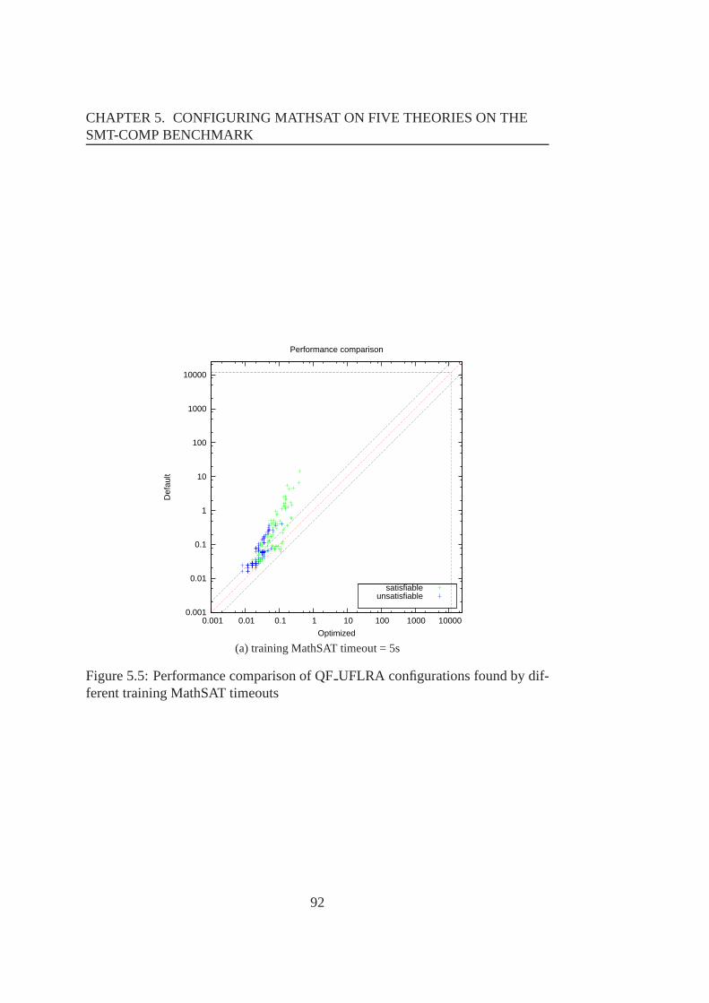
CHAPTER 5. CONFIGURING MATHSAT ON FIVE THEORIES ON THESMT-COMP BENCHMARK
0.001
0.01
0.1
1
10
100
1000
10000
0.001 0.01 0.1 1 10 100 1000 10000
Def
ault
Optimized
Performance comparison
satisfiableunsatisfiable
(a) training MathSAT timeout = 5s
Figure 5.5: Performance comparison of QFUFLRA configurations found by dif-ferent training MathSAT timeouts
92

5.5. QFUFLRA WITH FOCUSED PARAMILS USING DAE
0.001
0.01
0.1
1
10
100
1000
10000
0.001 0.01 0.1 1 10 100 1000 10000
Def
ault
Optimized
Performance comparison
satisfiableunsatisfiable
(b) training MathSAT timeout = 10s
0.001
0.01
0.1
1
10
100
1000
10000
0.001 0.01 0.1 1 10 100 1000 10000
Def
ault
Optimized
Performance comparison
satisfiableunsatisfiable
(c) training MathSAT timeout = 15s
Figure 5.5: Performance comparison of QFUFLRA configurations found by dif-ferent training MathSAT timeouts (cont.)
93
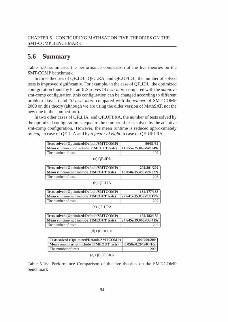
CHAPTER 5. CONFIGURING MATHSAT ON FIVE THEORIES ON THESMT-COMP BENCHMARK
5.6 Summary
Table 5.16 summaries the performance comparison of the five theories on theSMT-COMP benchmark.
In three theories of QFIDL, QF LRA, and QFUFIDL, the number of solvedtests is improved significantly. For example, in the case of QF IDL, the optimizedconfiguration found by ParamILS solves14 tests morecompared with theadaptivesmt-comp configuration (this configuration can be changed according to differentproblem classes) and10 tests morecompared with thewinner of SMT-COMP2009 on this theory (although we are using the older version of MathSAT, not thenew one in the competition).
In two other cases of QFLIA, and QF UFLRA, the number of tests solved bythe optimized configuration is equal to the number of tests solved by the adaptivesmt-comp configuration. However, the mean runtime is reduced approximatelyby half in case of QFLIA and bya factor of eightin case of QFUFLRA.
Tests solved (Optimized/Default/SMTCOMP) 96/81/82Mean runtime (not include TIMEOUT tests) 14.755s/25.069s/40.349sThe number of tests 102
(a) QF IDL
Tests solved (Optimized/Default/SMTCOMP) 202/201/202Mean runtime(not include TIMEOUT tests) 13.850s/15.495s/26.322sThe number of tests 205
(b) QF LIA
Tests solved (Optimized/Default/SMTCOMP) 184/177/183Mean runtime(not include TIMEOUT tests) 27.641s/35.057s/19.177sThe number of tests 202
(c) QF LRA
Tests solved (Optimized/Default/SMTCOMP) 192/182/189Mean runtime(not include TIMEOUT tests) 24.645s/39.063s/33.415sThe number of tests 202
(d) QF UFIDL
Tests solved (Optimized/Default/SMTCOMP) 200/200/200Mean runtime(not include TIMEOUT tests) 0.056s/0.204s/0.410sThe number of tests 200
(e) QFUFLRA
Table 5.16: Performance Comparison of the five theories on the SMT-COMPbenchmark
94

Chapter 6
Configuring on Other Theories onthe SMT-COMP Benchmark
This chapter summaries the experimental results on the three other theories QFUFLIA,QF UF, QF RDL. In these theories, we found bugs in the testing phase this is dueto the fact that in the training phase, we use not only the tested parameter but alsothe internal parameterswhich were used by developers and not tested carefully.
Before moving to the next sections of experiments, we introduce briefly thethree theories experimented in this chapter:
• QF UF: Unquantified formulas built over a signature of uninterpreted (i.e.,free) sort and function symbols. For example:{(f(x1) = f(x2)),¬(f(x2) =f(x3))}.
• QF RDL Difference Logic over the reals. In essence, Boolean combina-tions of inequations of the form(x−y < b) where x and y are real variablesand b is a rational constant.
• QF UFLIA : Unquantified linear integer arithmetic with uninterpreted sortand function symbols.
95

CHAPTER 6. CONFIGURING ON OTHER THEORIES ON THESMT-COMP BENCHMARK
6.1 QF UFLIA with Focused ParamILS using DAE
6.1.1 Experimental setup
CPU Intel(R) Xeon(R) CPU E5430 @ 2.66GHzOperating system Debian 5.0.4MathSAT version v4.2.10-itp (May 12 2010 08:54:51, gmp 4.3.2, gcc 4.4.3)Training MathSAT timeout 1 50s (the smt-comp configuration solved 98.01% of tests)Training MathSAT timeout 2 55s (the smt-comp configuration solved 98.01% of tests)Training MathSAT timeout 3 60s (the smt-comp configuration solved 98.51% of tests)Testing MathSAT timeout 1200sTraining time 48 hoursTraining set the QFUFLIA of SMT-COMP 2009Testing set Training setParamILS Configuration Focused, deterministic=1, N=202
run obj=runtime, overallobj=mean
Table 6.1: The experimental setup of QFUFLIA with different training MathSATtimeouts
6.1.2 Experimental result
Testing bugs:In testing phase, we found many inconsistent results. For example:bin/mathsat -input=smt -solve -logic=QFUFLIA data/QFUFLIA/wisas/xs16 36.smt
returns UNSAT.bin/mathsat -input=smt -solve -deduction=2 -implexpl threshold=0 -noaep -
dual rail=off -no pure literal filter -randomdecisions -spliteq -noincr tsolvers-tsolver=dl -tsolver=laz -dynack -dynack limit=0 -dyn ack threshold=10 -noexpensiveccmin-no frequentreducedb -noghostfilter -no ibliwi -mixed cs -permanenttheory lemmas-restarts=adaptive -sl=0 -tcomb=dtc -toplevelprop=2 data/QF UFLIA/wisas/xs16 36.smtreturns SAT.
96
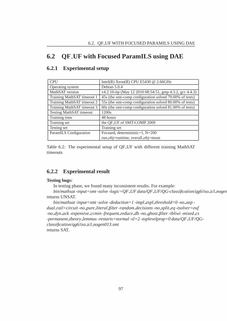
6.2. QFUF WITH FOCUSED PARAMILS USING DAE
6.2 QF UF with Focused ParamILS using DAE
6.2.1 Experimental setup
CPU Intel(R) Xeon(R) CPU E5430 @ 2.66GHzOperating system Debian 5.0.4MathSAT version v4.2.10-itp (May 12 2010 08:54:51, gmp 4.3.2, gcc 4.4.3)Training MathSAT timeout 1 45s (the smt-comp configuration solved 79.00% of tests)Training MathSAT timeout 2 55s (the smt-comp configuration solved 80.00% of tests)Training MathSAT timeout 3 60s (the smt-comp configuration solved 81.00% of tests)Testing MathSAT timeout 1200sTraining time 48 hoursTraining set the QFUF of SMT-COMP 2009Testing set Training setParamILS Configuration Focused, deterministic=1, N=200
run obj=runtime, overallobj=mean
Table 6.2: The experimental setup of QFUF with different training MathSATtimeouts
6.2.2 Experimental result
Testing bugs:In testing phase, we found many inconsistent results. For example:bin/mathsat -input=smt -solve -logic=QFUF data/QFUF/QG-classification/qg6/isoicl nogen0
returns UNSAT.bin/mathsat -input=smt -solve -deduction=1 -implexpl threshold=0 -noaep -
dual rail=circuit -no pure literal filter -randomdecisions -nosplit eq -tsolver=euf-no dyn ack -expensiveccmin -frequentreducedb -noghostfilter -ibliwi -mixed cs-permanenttheory lemmas -restarts=normal -sl=2 -toplevelprop=0 data/QFUF/QG-classification/qg6/isoicl nogen013.smtreturns SAT.
97

CHAPTER 6. CONFIGURING ON OTHER THEORIES ON THESMT-COMP BENCHMARK
6.3 QF RDL with Focused ParamILS using DAE
6.3.1 Experimental setup
CPU Intel(R) Xeon(R) CPU E5430 @ 2.66GHzOperating system Debian 5.0.4MathSAT version v4.2.10-itp (May 12 2010 08:54:51, gmp 4.3.2, gcc 4.4.3)Training MathSAT timeout 1 50s (the smt-comp configuration solved 86.85% of tests)Training MathSAT timeout 2 55s (the smt-comp configuration solved 88.00% of tests)Training MathSAT timeout 3 60s (the smt-comp configuration solved 89.14% of tests)Testing MathSAT timeout 1200sTraining time 48 hoursTraining set the QFRDL of SMT-COMP 2009Testing set Training setParamILS Configuration Focused, deterministic=1, N=175
run obj=runtime, overallobj=mean
Table 6.3: The experimental setup of QFRDL with different training MathSATtimeouts
6.3.2 Experimental result
Testing bugs:In testing phase, we found many inconsistent results of MathSAT on the same
test. For example:bin/mathsat -input=smt -solve -logic=QFRDL data/QFRDL/sal/fischer6-mutex-
20.smtreturns UNSAT.
bin/mathsat -input=smt -solve -deduction=0 -implexpl threshold=0 -aep -randomdecisions -nosplit eq -tsolver=euf -tsolver=dl -expensiveccmin -frequentreducedb-ghostfilter -dual rail=off -no pure literal filter -ibliwi -no mixedcs -permanenttheory lemmas-restarts=normal -sl=0 -toplevelprop=2 data/QFRDL/sal/fischer9-mutex-20.smtreturns SAT.
98

Chapter 7
More Results of the Five Theories onthe SMT-LIB Benchmark
This section shows the results of using ParamILS to find the best possible con-figurations for the five theories having no bugs (in Chapter 5)on the SMT-LIBbenchmark. The experiments in this section usedifferent datasetsof SMT-LIBfor training and testing because we want to get the best possible MathSAT con-figurations forgeneral cases. For each theory, a training dataset is extracted fromSMT-LIB by using the benchmark selection tool of SMT-COMP 2009. Then,we remove that training dataset from SMT-LIB, and extract another dataset fortesting.
The experiment setup for all tests in this chapter is summarised as follows:Based on the experimental results in Chapter 4, Focused ParamILS using DAE isthe best strategy for MathSAT. In addition, the training time of 48 hours is enoughfor MathSAT to converge with the MathSAT timeouts less than 60 seconds. Asfor choosing the training MathSAT timeouts, we run MathSAT with the smtcompconfiguration on the training dataset in advance and choose the three MathSATtimeouts (all timeouts have value from 0 to 1200 with step 5) which are less than60 seconds and solve similar percentage of tests.
Notice that the smt-comp configurations areadaptive, i.e. they can be changedaccording to different problem classes based on a statistics module in MathSAT.
99
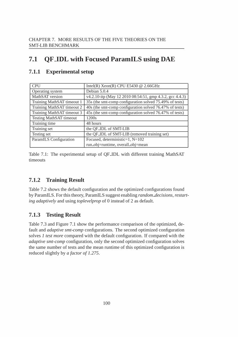
CHAPTER 7. MORE RESULTS OF THE FIVE THEORIES ON THESMT-LIB BENCHMARK
7.1 QF IDL with Focused ParamILS using DAE
7.1.1 Experimental setup
CPU Intel(R) Xeon(R) CPU E5430 @ 2.66GHzOperating system Debian 5.0.4MathSAT version v4.2.10-itp (May 12 2010 08:54:51, gmp 4.3.2, gcc 4.4.3)Training MathSAT timeout 1 35s (the smt-comp configuration solved 75.49% of tests)Training MathSAT timeout 2 40s (the smt-comp configuration solved 76.47% of tests)Training MathSAT timeout 3 45s (the smt-comp configuration solved 76.47% of tests)Testing MathSAT timeout 1200sTraining time 48 hoursTraining set the QFIDL of SMT-LIBTesting set the QFIDL of SMT-LIB (removed training set)ParamILS Configuration Focused, deterministic=1, N=102
run obj=runtime, overallobj=mean
Table 7.1: The experimental setup of QFIDL with different training MathSATtimeouts
7.1.2 Training Result
Table 7.2 shows the default configuration and the optimized configurations foundby ParamILS. For this theory, ParamILS suggest enablingrandomdecisions, restart-ing adaptivelyand usingtoplevelpropof 0 instead of 2 as default.
7.1.3 Testing Result
Table 7.3 and Figure 7.1 show the performance comparison of the optimized, de-fault andadaptive smt-compconfigurations. The second optimized configurationsolves1 test morecompared with the default configuration. If compared with theadaptive smt-compconfiguration, only the second optimized configuration solvesthe same number of tests and the mean runtime of this optimized configuration isreduced slightly bya factor of 1.275.
100

7.1. QFIDL WITH FOCUSED PARAMILS USING DAE
Configuration Default 35s 40s 45sParameteraep yes yes yes yesdeduction 2 2 2 1dual rail off off off offdyn ack no no no nodyn ack limit 0 0 0 0dyn ack threshold 1 1 1 1expensiveccmin yes yes yes yesfrequentreducedb no no no noghostfilter no no no noibliwi yes no yes noimpl expl threshold 0 0 0 0incr tsolvers no no no nomixed cs yes yes yes yespermanenttheory lemmas yes yes yes yespure literal filter no no no norandom decisions no no yes yesrestarts normal adaptive adaptive quicksl 2 2 2 2split eq yes yes yes yestcomb off off off offtoplevelprop 1 2 0 0tsolver dl dl dl dl
Table 7.2: QFIDL configurations found by different training MathSAT timeouts
101

CHAPTER 7. MORE RESULTS OF THE FIVE THEORIES ON THESMT-LIB BENCHMARK
Tests solved (Optimized/Default/SMTCOMP) 94/94/95Mean runtime (not include TIMEOUT tests) 1.848s/2.744s/6.410sOptimized compared with Default ResultBetter runtime tests/The number of tests 60/100Equal runtime tests/The number of tests 29/100Worse runtime tests/The number of tests 11/100
(a) training MathSAT timeout = 35s
Tests solved (Optimized/Default/SMTCOMP) 95/94/95Mean runtime(not include TIMEOUT tests) 5.207s/2.744s/6.410sOptimized compared with Default ResultBetter runtime tests/The number of tests 50/100Equal runtime tests/The number of tests 12/100Worse runtime tests/The number of tests 38/100
(b) training MathSAT timeout = 40s
Tests solved (Optimized/Default/SMTCOMP) 94/94/95Mean runtime(not include TIMEOUT tests) 1.352s/2.744s/6.410sOptimized compared with Default ResultBetter runtime tests/The number of tests 42/100Equal runtime tests/The number of tests 14/100Worse runtime tests/The number of tests 44/100
(c) training MathSAT timeout = 45s
Table 7.3: Performance comparison of QFIDL configurations found by differenttraining MathSAT timeouts
102

7.1. QFIDL WITH FOCUSED PARAMILS USING DAE
0.001
0.01
0.1
1
10
100
1000
10000
0.001 0.01 0.1 1 10 100 1000 10000
Def
ault
Optimized
Performance comparison
satisfiableunsatisfiableerror/timeout
(a) training MathSAT timeout = 35s
Figure 7.1: Performance comparison of QFIDL configurations found by differenttraining MathSAT timeouts
103

CHAPTER 7. MORE RESULTS OF THE FIVE THEORIES ON THESMT-LIB BENCHMARK
0.001
0.01
0.1
1
10
100
1000
10000
0.001 0.01 0.1 1 10 100 1000 10000
Def
ault
Optimized
Performance comparison
satisfiableunsatisfiableerror/timeout
(b) training MathSAT timeout = 40s
0.001
0.01
0.1
1
10
100
1000
10000
0.001 0.01 0.1 1 10 100 1000 10000
Def
ault
Optimized
Performance comparison
satisfiableunsatisfiableerror/timeout
(c) training MathSAT timeout = 45s
Figure 7.1: Performance comparison of QFIDL configurations found by differenttraining MathSAT timeouts (cont.)
104

7.2. QFLIA WITH FOCUSED PARAMILS USING DAE
7.2 QF LIA with Focused ParamILS using DAE
7.2.1 Experimental setup
CPU Intel(R) Xeon(R) CPU E5430 @ 2.66GHzOperating system Debian 5.0.4MathSAT version v4.2.10-itp (May 12 2010 08:54:51, gmp 4.3.2, gcc 4.4.3)Training MathSAT timeout 1 50s (the smt-comp configuration solved 83.41% of tests)Training MathSAT timeout 2 55s (the smt-comp configuration solved 83.90% of tests)Training MathSAT timeout 3 60s (the smt-comp configuration solved 85.58% of tests)Testing MathSAT timeout 1200sTraining time 48 hoursTraining set the QFLIA of SMT-LIBTesting set the QFLIA of SMT-LIB (remove training set)ParamILS Configuration Focused, deterministic=1, N=205
run obj=runtime, overallobj=mean
Table 7.4: The experimental setup of QFLIA with different training MathSATtimeouts
7.2.2 Training Result
Table 7.5 shows the default configuration and the optimized configuration foundby ParamILS. For QFLIA, ParamILS suggest usingimpl expl thresholdof 1 in-stead of 0,sl of 0 instead of 2,toplevelpropof 1, enablingincr tsolversand dis-ablingsplit eq.
7.2.3 Testing Result
Table 7.6 and Figure 7.2 of the optimized, default andadaptive smt-compconfig-urations. Although only in two of three cases, the optimizedconfigurations solvethe same number of tests compared with the default and the adaptive smt-compconfigurations, the mean runtime of the optimized configurations are reduced ap-proximately bya factor of 1.35, 3.56compared with the mean runtime of thedefault and smt-comp configuration, respectively.
105
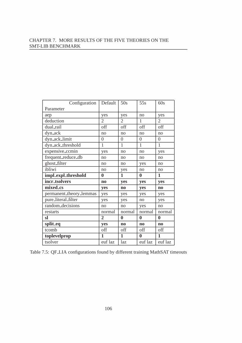
CHAPTER 7. MORE RESULTS OF THE FIVE THEORIES ON THESMT-LIB BENCHMARK
Configuration Default 50s 55s 60sParameteraep yes yes no yesdeduction 2 2 1 2dual rail off off off offdyn ack no no no nodyn ack limit 0 0 0 0dyn ack threshold 1 1 1 1expensiveccmin yes no no yesfrequentreducedb no no no noghostfilter no no yes noibliwi no yes no noimpl expl threshold 0 1 0 1incr tsolvers no yes yes yesmixed cs yes no yes nopermanenttheory lemmas yes yes yes yespure literal filter yes yes no yesrandomdecisions no no yes norestarts normal normal normal normalsl 2 0 0 0split eq yes no no notcomb off off off offtoplevelprop 1 1 0 1tsolver euf laz laz euf laz euf laz
Table 7.5: QFLIA configurations found by different training MathSAT timeouts
106

7.2. QFLIA WITH FOCUSED PARAMILS USING DAE
Tests solved (Optimized/Default/SMTCOMP) 199/199/199Mean runtime (not include TIMEOUT tests) 12.456s/17.369s/44.378sOptimized compared with Default ResultBetter runtime tests/The number of tests 181/200Equal runtime tests/The number of tests 5/200Worse runtime tests/The number of tests 14/200
(a) training MathSAT timeout = 50s
Tests solved (Optimized/Default/SMTCOMP) 198/199/199Mean runtime(not include TIMEOUT tests) 12.791s/17.369s/44.378sOptimized compared with Default ResultBetter runtime tests/The number of tests 148/200Equal runtime tests/The number of tests 8/200Worse runtime tests/The number of tests 44/200
(b) training MathSAT timeout = 55s
Tests solved (Optimized/Default/SMTCOMP) 199/199/199Mean runtime(not include TIMEOUT tests) 12.069s/17.369s/44.378sOptimized compared with Default ResultBetter runtime tests/The number of tests 183/200Equal runtime tests/The number of tests 8/200Worse runtime tests/The number of tests 9/200
(c) training MathSAT timeout = 60s
Table 7.6: Performance comparison of QFLIA configurations found by differenttraining MathSAT timeouts
107

CHAPTER 7. MORE RESULTS OF THE FIVE THEORIES ON THESMT-LIB BENCHMARK
0.001
0.01
0.1
1
10
100
1000
10000
0.001 0.01 0.1 1 10 100 1000 10000
Def
ault
Optimized
Performance comparison
satisfiableunsatisfiableerror/timeout
(a) training MathSAT timeout = 50s
Figure 7.2: Performance comparison of QFLIA configurations found by differenttraining MathSAT timeouts
108

7.2. QFLIA WITH FOCUSED PARAMILS USING DAE
0.001
0.01
0.1
1
10
100
1000
10000
0.001 0.01 0.1 1 10 100 1000 10000
Def
ault
Optimized
Performance comparison
satisfiableunsatisfiableerror/timeout
(b) training MathSAT timeout = 55s
0.001
0.01
0.1
1
10
100
1000
10000
0.001 0.01 0.1 1 10 100 1000 10000
Def
ault
Optimized
Performance comparison
satisfiableunsatisfiableerror/timeout
(c) training MathSAT timeout = 60s
Figure 7.2: Performance comparison of QFLIA configurations found by differenttraining MathSAT timeouts (cont.)
109

CHAPTER 7. MORE RESULTS OF THE FIVE THEORIES ON THESMT-LIB BENCHMARK
7.3 QF LRA with Focused ParamILS using DAE
7.3.1 Experimental setup
CPU Intel(R) Xeon(R) CPU E5430 @ 2.66GHzOperating system Debian 5.0.4MathSAT version v4.2.10-itp (May 12 2010 08:54:51, gmp 4.3.2, gcc 4.4.3)Training MathSAT timeout 1 40s (the smt-comp configuration solved 85.64 % of tests)Training MathSAT timeout 2 45s (the smt-comp configuration solved 86.13% of tests)Training MathSAT timeout 3 50s (the smt-comp configuration solved 86.63% of tests)Testing MathSAT timeout 1200sTraining time 48 hoursTraining set the QFLRA of SMT-LIBTesting set the QFLRA of SMT-LIB (removed training set)ParamILS Configuration Focused, deterministic=1, N=202
run obj=runtime, overallobj=mean
Table 7.7: The experimental setup of QFLRA with different training MathSATtimeouts
7.3.2 Training Result
Table 7.8 shows the default configuration and the optimized configurations foundby ParamILS. For QFLRA, ParamILS suggests disablingaep, pure literal filter,enablingsplit eqand using only one theory solverla.
7.3.3 Testing Result
Table 7.9 and Figure 7.3 show the performance comparison of the optimized, deaf-ault andadaptive smt-compconfiguration. Only the second optimized configura-tion has the same number of solved tests as the smt-comp configuration. However,if compared with the default configuration, the optimized configurations solve6,or 7 tests more.
110

7.3. QFLRA WITH FOCUSED PARAMILS USING DAE
Configuration Default 40s 45s 50sParameteraep yes no no nodeduction 2 2 2 2dual rail off off off offdyn ack no no no nodyn ack limit 0 0 0 0dyn ack threshold 1 1 1 1expensiveccmin yes yes yes yesfrequentreducedb no no no yesghostfilter no no yes noibliwi no no no noimpl expl threshold 0 0 0 1incr tsolvers no no no nomixed cs yes no no nopermanenttheory lemmas yes yes yes yespure literal filter yes no no yesrandomdecisions no no no norestarts normal normal normal normalsl 2 2 2 2split eq no yes yes yestcomb off off off offtoplevelprop 1 1 1 1tsolver euf la la la la
Table 7.8: QFLRA configurations found by different training MathSAT timeouts
111

CHAPTER 7. MORE RESULTS OF THE FIVE THEORIES ON THESMT-LIB BENCHMARK
Tests solved (Optimized/Default/SMTCOMP) 199/193/200Mean runtime(not include TIMEOUT tests) 11.099s/31.269s/9.033sOptimized compared with Default ResultBetter runtime tests/The number of tests 88/200Equal runtime tests/The number of tests 23/200Worse runtime tests/The number of tests 89/200
(a) training MathSAT timeout = 40s
Tests solved (Optimized/Default/SMTCOMP) 200/193/200Mean runtime(not include TIMEOUT tests) 19.759s/31.269s/9.033sOptimized compared with Default ResultBetter runtime tests/The number of tests 90/200Equal runtime tests/The number of tests 18/200Worse runtime tests/The number of tests 92/200
(b) training MathSAT timeout = 45s
Tests solved (Optimized/Default/SMTCOMP) 199/193/200Mean runtime(not include TIMEOUT tests) 13.799s/31.269s/9.033sOptimized compared with Default ResultBetter runtime tests/The number of tests 65/200Equal runtime tests/The number of tests 17/200Worse runtime tests/The number of tests 118/200
(c) training MathSAT timeout = 50s
Table 7.9: Performance comparison of QFLRA configurations found by differenttraining MathSAT timeouts
112
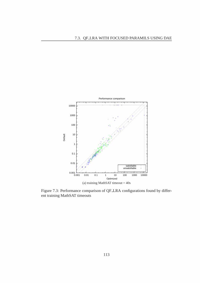
7.3. QFLRA WITH FOCUSED PARAMILS USING DAE
0.001
0.01
0.1
1
10
100
1000
10000
0.001 0.01 0.1 1 10 100 1000 10000
Def
ault
Optimized
Performance comparison
satisfiableunsatisfiable
(a) training MathSAT timeout = 40s
Figure 7.3: Performance comparison of QFLRA configurations found by differ-ent training MathSAT timeouts
113

CHAPTER 7. MORE RESULTS OF THE FIVE THEORIES ON THESMT-LIB BENCHMARK
0.001
0.01
0.1
1
10
100
1000
10000
0.001 0.01 0.1 1 10 100 1000 10000
Def
ault
Optimized
Performance comparison
satisfiableunsatisfiable
(b) training MathSAT timeout = 45s
0.001
0.01
0.1
1
10
100
1000
10000
0.001 0.01 0.1 1 10 100 1000 10000
Def
ault
Optimized
Performance comparison
satisfiableunsatisfiable
(c) training MathSAT timeout = 50s
Figure 7.3: Performance comparison of QFLRA configurations found by differ-ent training MathSAT timeouts (cont.)
114

7.4. QFUFIDL WITH FOCUSED PARAMILS USING DAE
7.4 QF UFIDL with Focused ParamILS using DAE
7.4.1 Experimental setup
CPU Intel(R) Xeon(R) CPU E5430 @ 2.66GHzOperating system Debian 5.0.4MathSAT version v4.2.10-itp (May 12 2010 08:54:51, gmp 4.3.2, gcc 4.4.3)Training MathSAT timeout 1 50s (the smt-comp configuration solved 82.67% of tests)Training MathSAT timeout 2 55s (the smt-comp configuration solved 83.66% of tests)Training MathSAT timeout 3 60s (the smt-comp configuration solved 84.65% of tests)Testing MathSAT timeout 1200sTraining time 48 hoursTraining set the QFUFIDL of SMT-LIBTesting set the QFUFIDL of SMT-LIB (removed training)ParamILS Configuration Focused, deterministic=1, N=202
run obj=runtime, overallobj=mean
Table 7.10: The experimental setup of QFUFIDL with different training Math-SAT timeouts
7.4.2 Training Result
Table 7.11 shows the default configuration and the optimizedconfigurations foundby ParamILS. The main difference between the optimized configurations andthe default configuration is that usingdeductionof 2 instead of 1, and enablingghostfilter instead of disabling as default.
7.4.3 Testing Result
Table 7.12 and Figure 7.4 show the performance comparison ofthe optimized,default andadaptive smt-compconfiguration. There is no optimized configurationhaving the number of solved tests greater than the number of tests solved by thesmt-comp configuration. However, if compared with the default configuration, theoptimized configurations solve11, 10, 6 tests more.
115

CHAPTER 7. MORE RESULTS OF THE FIVE THEORIES ON THESMT-LIB BENCHMARK
Configuration Default 50s 55s 60sParameteraep yes yes no nodeduction 2 1 1 1dual rail off off off offdyn ack no yes no nodyn ack limit 0 0 0 0dyn ack threshold 1 1 1 1expensiveccmin yes yes yes nofrequentreducedb no no no yesghost filter no yes yes yesibliwi yes yes yes yesimpl expl threshold 0 1 0 1incr tsolvers no no no nomixed cs yes yes no nopermanenttheory lemmas yes yes yes yespure literal filter no no no norandomdecisions no no yes yesrestarts normal quick normal adaptivesl 2 2 0 1split eq yes yes yes yestcomb dtc dtc decide decidetoplevelprop 1 1 1 0tsolver euf dl euf dl euf dl euf dl
Table 7.11: QFUFIDL configurations found by different training MathSAT time-outs
116
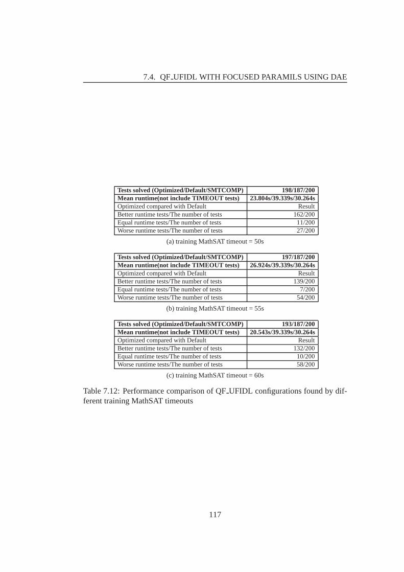
7.4. QFUFIDL WITH FOCUSED PARAMILS USING DAE
Tests solved (Optimized/Default/SMTCOMP) 198/187/200Mean runtime(not include TIMEOUT tests) 23.804s/39.339s/30.264sOptimized compared with Default ResultBetter runtime tests/The number of tests 162/200Equal runtime tests/The number of tests 11/200Worse runtime tests/The number of tests 27/200
(a) training MathSAT timeout = 50s
Tests solved (Optimized/Default/SMTCOMP) 197/187/200Mean runtime(not include TIMEOUT tests) 26.924s/39.339s/30.264sOptimized compared with Default ResultBetter runtime tests/The number of tests 139/200Equal runtime tests/The number of tests 7/200Worse runtime tests/The number of tests 54/200
(b) training MathSAT timeout = 55s
Tests solved (Optimized/Default/SMTCOMP) 193/187/200Mean runtime(not include TIMEOUT tests) 20.543s/39.339s/30.264sOptimized compared with Default ResultBetter runtime tests/The number of tests 132/200Equal runtime tests/The number of tests 10/200Worse runtime tests/The number of tests 58/200
(c) training MathSAT timeout = 60s
Table 7.12: Performance comparison of QFUFIDL configurations found by dif-ferent training MathSAT timeouts
117

CHAPTER 7. MORE RESULTS OF THE FIVE THEORIES ON THESMT-LIB BENCHMARK
0.001
0.01
0.1
1
10
100
1000
10000
0.001 0.01 0.1 1 10 100 1000 10000
Def
ault
Optimized
Performance comparison
satisfiableunsatisfiableerror/timeout
(a) training MathSAT timeout = 50s
Figure 7.4: Performance comparison of QFUFIDL configurations found by dif-ferent training MathSAT timeouts
118

7.4. QFUFIDL WITH FOCUSED PARAMILS USING DAE
0.001
0.01
0.1
1
10
100
1000
10000
0.001 0.01 0.1 1 10 100 1000 10000
Def
ault
Optimized
Performance comparison
satisfiableunsatisfiableerror/timeout
(b) training MathSAT timeout = 55s
0.001
0.01
0.1
1
10
100
1000
10000
0.001 0.01 0.1 1 10 100 1000 10000
Def
ault
Optimized
Performance comparison
satisfiableunsatisfiableerror/timeout
(c) training MathSAT timeout = 60s
Figure 7.4: Performance comparison of QFUFIDL configurations found by dif-ferent training MathSAT timeouts (cont.)
119

CHAPTER 7. MORE RESULTS OF THE FIVE THEORIES ON THESMT-LIB BENCHMARK
7.5 QF UFLRA with Focused ParamILS using DAE
7.5.1 Experimental setup
CPU Intel(R) Xeon(R) CPU E5430 @ 2.66GHzOperating system Debian 5.0.4MathSAT version v4.2.10-itp (May 12 2010 08:54:51, gmp 4.3.2, gcc 4.4.3)Training MathSAT timeout 1 5s (the smt-comp configuration solved 100% of tests)Training MathSAT timeout 2 10s (the smt-comp configuration solved 100% of tests)Training MathSAT timeout 3 15s (the smt-comp configuration solved 100% of tests)Testing MathSAT timeout 1200sTraining time 48 hoursTraining set the QFUFLRA of SMT-LIBTesting set the QFUFLRA of SMT-LIB (removed training)ParamILS Configuration Focused, deterministic=1, N=200
run obj=runtime, overallobj=mean
Table 7.13: The experimental setup of QFUFLRA with different training Math-SAT timeouts
7.5.2 Training Result
Table 7.14 shows the default configuration and the optimizedconfigurations foundParamILS. For QFUFLRA, ParamILS recommends users to enabledyn ack, fre-quentreducedb, ghostfilter, incr tsolversand disablepure literal filter. ParamILSalso suggests usingdeductionof 1,dyn ack thresholdof 50, or 10,slof 0, toplevel-propof 0.
7.5.3 Testing Result
Table 7.15 and Figure 7.5 show the performance comparison ofthe optimized,default andadaptive smt-compconfigurations. It can be seen that in call cases,the mean runtime of the optimized configurations are reducedapproximately bya factor of 6.678 and 3.375compared with the mean runtime of the default, andsmt-comp configuration.
120

7.5. QFUFLRA WITH FOCUSED PARAMILS USING DAE
Configuration Default 5s 10s 15sParameteraep yes yes yes yesdeduction 2 1 1 1dual rail off off off offdyn ack no yes yes yesdyn ack limit 0 0 0 0dyn ack threshold 1 50 50 10expensiveccmin yes yes no yesfrequent reduce db no yes yes yesghost filter no yes yes yesibliwi no no no noimpl expl threshold 0 0 0 0incr tsolvers no yes yes yesmixed cs yes yes yes yespermanenttheory lemmas yes yes no yespure literal filter yes no no norandomdecisions no no no norestarts normal normal normal normalsl 2 0 0 0split eq no no no notcomb dtc dtc dtc dtctoplevelprop 1 0 0 0tsolver euf la euf la euf la euf la
Table 7.14: QFUFLRA configurations found by different training MathSATtimeouts
121

CHAPTER 7. MORE RESULTS OF THE FIVE THEORIES ON THESMT-LIB BENCHMARK
Tests solved (Optimized/Default/SMTCOMP) 200/200/200Mean runtime(not include TIMEOUT tests) 0.057s/0.374s/0.189sOptimized compared with Default ResultBetter runtime tests/The number of tests 193/200Equal runtime tests/The number of tests 4/200Worse runtime tests/The number of tests 3/200
(a) training MathSAT timeout = 5s
Tests solved (Optimized/Default/SMTCOMP) 200/200/200Mean runtime(not include TIMEOUT tests) 0.059s/0.374s/0.189sOptimized compared with Default ResultBetter runtime tests/The number of tests 189/200Equal runtime tests/The number of tests 4/200Worse runtime tests/The number of tests 7/200
(b) training MathSAT timeout = 10s
Tests solved (Optimized/Default/SMTCOMP) 200/200/200Mean runtime(not include TIMEOUT tests) 0.056s/0.374s/0.189sOptimized compared with Default ResultBetter runtime tests/The number of tests 192/200Equal runtime tests/The number of tests 5/200Worse runtime tests/The number of tests 3/200
(c) training MathSAT timeout = 15s
Table 7.15: Performance comparison of QFUFLRA configurations found by dif-ferent training MathSAT timeouts
122

7.5. QFUFLRA WITH FOCUSED PARAMILS USING DAE
0.001
0.01
0.1
1
10
100
1000
10000
0.001 0.01 0.1 1 10 100 1000 10000
Def
ault
Optimized
Performance comparison
satisfiableunsatisfiable
(a) training MathSAT timeout = 5s
Figure 7.5: Performance comparison of QFUFLRA configurations found by dif-ferent training MathSAT timeouts
123

CHAPTER 7. MORE RESULTS OF THE FIVE THEORIES ON THESMT-LIB BENCHMARK
0.001
0.01
0.1
1
10
100
1000
10000
0.001 0.01 0.1 1 10 100 1000 10000
Def
ault
Optimized
Performance comparison
satisfiableunsatisfiable
(b) training MathSAT timeout = 10s
0.001
0.01
0.1
1
10
100
1000
10000
0.001 0.01 0.1 1 10 100 1000 10000
Def
ault
Optimized
Performance comparison
satisfiableunsatisfiable
(c) training MathSAT timeout = 15s
Figure 7.5: Performance comparison of QFUFLRA configurations found by dif-ferent training MathSAT timeouts (cont.)
124

7.6. SUMMARY
7.6 Summary
Table 7.16 summaries the performance comparison of the five theories on theSMT-LIB benchmark.
In four theories of QFIDL, QF LIA, QF LRA, and QFUFLRA, the num-ber of tests solved by the optimized configuration is equal tothe number of testssolved by theadaptivesmt-comp configuration (this configuration can be changedaccording to different problem classes) and is larger than the number of testssolved by the default configurations. In addition, the mean runtime is reducedby a factor of1.231in case of QFIDL, by a factor of3.677 in case of QFLIA,and by a factor of3.375 in case of QFUFLRA. Only in the case of QFLRA,the mean runtime of the optimized configuration is increasedby a factor of2.187compared with the mean runtime of the adaptive smt-comp configuration. Butif compared with the default configuration, the optimized configuration solves7tests more.
In the case of QFUFIDL, the optimized configuration solves2 tests lesscom-pared with the adaptive smt-comp configuration. However, ifcompared with thedefault configuration, the optimized configuration solves11 tests more.
125

CHAPTER 7. MORE RESULTS OF THE FIVE THEORIES ON THESMT-LIB BENCHMARK
Tests solved (Optimized/Default/SMTCOMP) 95/94/95Mean runtime(not include TIMEOUT tests) 5.207s/2.744s/6.410sThe number of tests 100
(a) QF IDL
Tests solved (Optimized/Default/SMTCOMP) 199/199/199Mean runtime(not include TIMEOUT tests) 12.069s/17.369s/44.378sThe number of tests 200
(b) QF LIA
Tests solved (Optimized/Default/SMTCOMP) 200/193/200Mean runtime(not include TIMEOUT tests) 19.759s/31.269s/9.033sThe number of tests 200
(c) QF LRA
Tests solved (Optimized/Default/SMTCOMP) 198/187/200Mean runtime(not include TIMEOUT tests) 23.804s/39.339s/30.264sThe number of tests 200
(d) QF UFIDL
Tests solved (Optimized/Default/SMTCOMP) 200/200/200Mean runtime(not include TIMEOUT tests) 0.056s/0.374s/0.189sThe number of tests 200
(e) QFUFLRA
Table 7.16: Performance Comparison of the five theories on the SMT-LIB bench-mark
126

Chapter 8
Conclusion
The main contribution of this thesis is a comprehensive study of the most effectiveSMT techniques. This includes an empirical analysis approach to study the char-acteristics of the MathSAT configuration scenario, two experimental groups oneight and five theories to determine the best possible configurations for MathSATon the SMT-COMP 2009 and SMT-LIB benchmark. Here, we describe these inmore detail:
• We have done many experiments on a theory to determine the most suitablescenario for MathSAT before starting experiments on a set oftheories. Themain parameters in a scenario are the ParamILS strategy (Basic or Focused),the timeout of ParamILS (tunnerTimeout), the timeout of each MathSATrun(cutoff time), the effect of ParamILS random seeds, the determinismofMathSAT. From the experimental results, we have concluded thatFocusedParamILS using DAEis the most suitable ParamILS for MathSAT. As forthe training time,48 hoursis enough for the ParamILS convergence becausewe have experimented on theQF LRA, one of the most difficult theoriesin the set of theories supported by MathSAT, and observed that ParamILSconverged within48 training hourswith the MathSAT timeouts less than60s. In order to choose suitable MathSAT timeouts when training, we haverun MathSAT with the default (or smt-comp) configuration on the trainingdataset in advance and chosen the three MathSAT timeouts (all timeoutshave value from 0 to 1200 with step 5) which are less than 60 seconds andsolve similar percentage of tests.
• Then, we have started ParamILS on eight theories using the SMT-COMP2009 benchmark. In these experiments, we have used the same dataset ofSMT-COMP 2009 for training and testing phases in order to check whetherwe could have better configurations than the default configurations and theconfigurations used in SMT-COMP 2009 (smt-comp configurations, these
127

CHAPTER 8. CONCLUSION
configurations could bechangedaccording to different problem classesbased on a statistics module in MathSAT). In three theories of QF IDL,QF LRA, and QFUFIDL, the number of solved tests is improved signif-icantly. For example, in the case of QFIDL, the optimized configurationfound by ParamILS solves14 tests morecompared with the adaptive smt-comp configuration and10 tests morecompared with thewinner of SMT-COMP 2009 on this theory (despite the fact that we are using the older ver-sion of MathSAT, not the new one in the competition). In two other casesof QF LIA, and QF UFLRA, the number of tests solved by the optimizedconfiguration is equal to the number of tests solved by the adaptive smt-comp configuration. However, the mean runtime is reduced approximatelyby half in case of QFLIA and by a factor of eightin case of QFUFLRA.For other three theories, we have encountered some bugs whentesting, andreport them to the MathSAT team because we used not only the tested pa-rameters but alsointernalparameters which are used for developers and nottested carefully.
• Next, we have used the benchmark selection tool of SMT-COMP 2009 toextract from the SMT-LIB benchmark different training and testing datasetsfor five successfully tested theories (no errors found in training and test-ing phases for these theories in Chapter 5) to find general optimized Math-SAT configurations. In four theories of QFIDL, QF LIA, QF LRA, andQF UFLRA, the number of tests solved by the optimized configuration isequal to the number of tests solved by theadaptivesmt-comp configurationand is larger than the number of tests solved by the default configurations.In addition, the mean runtime is reduced by a factor of1.231 in case ofQF IDL, by a factor of3.677 in case of QFLIA, and by a factor of3.375in case of QFUFLRA. Only in the case of QFLRA, the mean runtime ofthe optimized configuration is increased by a factor of2.187compared withthe mean runtime of the adaptive smt-comp configuration. Butif comparedwith the default configuration, the optimized configurationsolves7 testsmore. In the case of QFUFIDL, the optimized configuration solves2 testslesscompared with the adaptive smt-comp configuration. However, if com-pared with the default configuration, the optimized configuration solves11tests more.
128

Chapter 9
List of Acronyms
• RAE Random Algorithm Evaluation (used in ParamILS).
• DAE Deterministic Algorithm Evaluation (used in ParamILS).
129

130

Bibliography
[1] Frank Hutter, Holger H. Hoos, and Thomas Stutzle. Automatic algorithmconfiguration based on local search. In AAAI, pages 11521157. AAAI Press,2007. 26
[2] Diplomarbeit In Englischer Sprache, Von Frank Hutter, and Betreuer Dr.Thomas Stutzle. Stochastic local search for solving the most probable expla-nation problem in bayesian networks, 2004. 26, 33
[3] Frank Hutter, Holger H. Hoos, Kevin Leyton-Brown, and Thomas Stutzle.ParamILS: An Automatic Algorithm Conguration Framework. In Journal ofArtificial Intelligence Research 36 (2009) 267-306, 2009. 21
[4] Roberto Sebastiani. Lazy Satisability Modulo Theories. JSAT, Vol. 3, Num-ber 3-4, pp. 141-224, 2007. 7, 8, 12, 13, 15, 17, 19
[5] Alberto Griggio. An effective SMT engine for Formal Verification. Ph.D.Thesis, DISI - University of Trento. 13
[6] Anders Franzn. Efficient Solving of the Satisfiability Modulo Bit-VectorsProblem and Some Extensions to SMT. Ph.D. Thesis, DISI - University ofTrento. 14
[7] Jinbo Huang. The Effect of Restarts on the Efficiency of Clause Learning.IJCAI, pp. 2318-2323, 2007. 18
[8] Armin Biere. Adaptive Restart Strategies for Conflict Driven SAT Solvers.SAT, Lecture Notes in Computer Science, Vol. 4996, pp. 28-33, Springer,2008. 19
[9] Alessandro Cimatti, Alberto Griggio and Roberto Sebastiani. Efficient Inter-polant Generation in Satisfiability Modulo Theories. ACM Transaction onComputational Logics, TOCL. To appear. Available from TOCLacceptedpapers web page. 17, 20
131
BIBLIOGRAPHY
[10] Dutertre, B., de Moura, L.: The Yices SMT Solver.http://yices.csl.sri.com/tool-paper.pdf (2006) 15
[11] Niklas Sorensson, Niklas Een. Minisat 1.13 system description,http://www.minisat.se/downloads/MiniSatv1.13 short.pdf. 15
[12] Clark Barrett, Roberto Sebastiani, Sanjit Seshia, Cesare Tinelli. SatisfiabilityModulo Theories. Part II, Chapter 26, The Handbook of Satisfiability. 2009.IOS press. 8
[13] Jan-Willem Roorda and Koen Claessen. SAT-Based assistance in abstractionrefinement for symbolic trajectory evaluation. In ComputerAided Verifica-tion, pages 175-189, Springer-Verlag, 2006. 13
[14] Bozzano, M., Bruttomsesso, R., Cimatti, A., Junttila,T., Van Rossum, P.,Ranise, S., And Sebastiani, R.. Efficient Theory Combination via BooleanSearch. Information and Computation 204, 10(October), 1411-1596, 2006.20
[15] Lourenco, H. R., Martin, O., & Stutzle, T. Iterated local search. In F.Glover & G. Kochenberger (Eds.), Handbook of Metaheuristics (pp. 321-353). Kluwer Academic Publishers, Norwell, MA, USA, 2002. 22
[16] Carsten Sinz and Markus Iser. Problem-Sensitive Restart Heuristics for theDPLL Procedure. SAT, Lecture Notes in Computer Science, Vol. 5584, pp.356-362, Springer, 2009. 18
[17] http://goedel.cs.uiowa.edu/smtlib/ 57
[18] W. Ackermann. Solvable Cases of the Decision Problem. North Holland Pub.Co., Amsterdam, 1954. 14
[19] A. Armando, C. Castellini, and E. Giunchiglia. SAT-based procedures fortemporal reasoning. In Proc. European Conference on Planning, CP-99,1999. 7, 9, 10, 13, 19
[20] A. Armando, C. Castellini, E. Giunchiglia, and M. Maratea. A SAT-basedDecision Procedure for the Boolean Combination of Difference Constraints.In Proc. SAT04, 2004. 7
[21] G. Audemard, P. Bertoli, A. Cimatti, A. Korni lowicz, and R. Sebastiani.A SAT Based Approach for Solving Formulas over Boolean and LinearMathematical Propositions. In Proc. CADE’2002., volume 2392 of LNAI.Springer, July 2002. 9, 10, 13, 17, 18
132

BIBLIOGRAPHY
[22] G. Audemard, M. Bozzano, A. Cimatti, and R. Sebastiani.Verifying In-dustrial Hybrid Systems with MathSAT. In Proc. BMC04, volume 89/4 ofENTCS. Elsevier, 2003. 7
[23] G. Audemard, A. Cimatti, A. Korni lowicz, and R. Sebastiani. SAT-BasedBounded Model Checking for Timed Systems. In Proc. FORTE02., volume2529 of LNCS. Springer, November 2002. 7, 19
[24] T. Ball, B. Cook, S. K. Lahiri, and L. Zhang. Zapato: Automatic Theo-rem Proving for Predicate Abstraction Refinement. In Proc. CAV04, volume3114 of LNCS. Springer, 2004. 7
[25] C. Barrett and S. Berezin. CVC Lite: A New Implementation of the Cooper-ating Validity Checker. In Proceedings of the 16th International Conferenceon Computer Aided Verification (CAV 04), volume 3114 of LNCS.Springer,2004. 7
[26] C. Barrett, L. de Moura, and A. Stump. SMT-COMP: Satisfiability ModuloTheories Competition. In Proc. CAV05, volume 3576 of LNCS. Springer,2005. 9
[27] C. Barrett, D. Dill, and A. Stump. Checking Satisfiability of First-Order For-mulas by Incremental Translation to SAT. In 14th International Conferenceon Computer-Aided Verification, 2002. 9
[28] C. W. Barrett, D. L. Dill, and A. Stump. A generalizationof Shostaksmethod for combining decision procedures. In Frontiers of Combining Sys-tems (FROCOS), LNAI. Springer, April 2002. S. Margherita Ligure, Italy.8
[29] C. W. Barrett, Y. Fang, B. Goldberg, Y. Hu, A. Pnueli, andL. D. Zuck.TVOC: A Translation Validator for Optimizing Compilers. InProc. CAV05,volume 3576 of LNCS. Springer, 2005. 7
[30] R. J. Bayardo and R. C. Schrag. Using CSP Look-Back Techniques to SolveReal-World SAT instances. In Proc. AAAI97, pages 203208. AAAI Press,1997. 8, 9, 16
[31] A. Biere, A. Cimatti, E. Clarke, and Y. Zhu. Symbolic model checking with-out BDDs. In Proc. CAV99, 1999. 8
[32] A. Boralv. A Fully Automated Approach for Proving Safety Properties inInter- locking Software Using Automatic Theorem-Proving.In Proceedingsof the Second International ERCIM Workshop on Formal Methods for In-dustrial Critical Systems, 1997. 8
133

BIBLIOGRAPHY
[33] M. Bozzano, R. Bruttomesso, A. Cimatti, A. Franzen, Z. Hanna, Z. Khasi-dashvili, A Palti, and R. Sebastiani. Encoding RTL Constructs for MathSAT:a Preliminary Report. In Proc. PDPAR05, volume 144 of ENTCS.Elsevier,2006. 7, 20
[34] M. Bozzano, R. Bruttomesso, A. Cimatti, T. Junttila, P.van Rossum, S.Schulz, and R. Sebastiani. An incremental and Layered Procedure for theSatisfiability of Linear Arithmetic Logic. In Proc. TACAS05, volume 3440of LNCS. Springer, 2005. 7, 9
[35] M. Bozzano, R. Bruttomesso, A. Cimatti, T. Junttila, P.van Rossum, S.Schulz, and R. Sebastiani. MathSAT: A Tight Integration of SAT and Mathe-matical Decision Procedure. Journal of Automated Reasoning, 35(1-3), Oc-tober 2005. 9, 17, 19
[36] M. Bozzano, R. Bruttomesso, A. Cimatti, T. Junttila, P.van Rossum,S. Ranise, and R. Sebastiani. Efficient Theory Combination via BooleanSearch. Information and Computation, 204(10), 2006. 10
[37] R. Brinkmann and R. Drechsler. RTL-datapath verification using integer lin-ear programming. In Proc. ASP-DAC 2002, pages 741-746. IEEE, 2002. 20
[38] R. E. Bryant, S. K. Lahiri, and S. A. Seshia. Modeling andVerifying Sys-tems Using a Logic of Counter Arithmetic with Lambda Expressions andUninterpreted Functions. In Proc. CAV02, volume 2404 of LNCS. Springer,2002. 9
[39] J. R. Burch and D. L. Dill. Automatic Verification of Pipelined Micropro-cessor Control. In Proc. CAV 94, volume 818 of LNCS. Springer, 1994. 7
[40] C. Castellini, E. Giunchiglia, and A. Tacchella. SAT-based planning in com-plex domains: Concurrency, constraints and nondeterminism. Artificial In-telligence, 147(12):85-117, 2003. 8
[41] M. Davis, G. Logemann, and D. Loveland. A machine program for theoremproving. Journal of the ACM, 5(7), 1962. 9
[42] M. Davis and H. Putnam. A computing procedure for quantification theory.Journal of the ACM, 7:201-215, 1960. 9
[43] L. de Moura and N. Bjrner. System Description: Z3 0.1. In3rd Int. Competition of Satisfiability Modulo Theories tools, 2007.http://research.microsoft.com/projects/z3/smtcomp07.pdf. 7
134

BIBLIOGRAPHY
[44] L. de Moura and H. Ruess. An Experimental Evaluation of Ground DecisionProcedures. In Proc. CAV04, volume 3114 of LNCS. Springer, 2004. 9
[45] L. de Moura, H. Rue, and M. Sorea. Lazy Theorem Proving for BoundedModel Checking over Infinite Domains. In Proc. of the 18th InternationalConference on Automated Deduction, volume 2392 of LNCS, pages 438-455. Springer, July 2002. 7, 9
[46] D. Detlefs, G. Nelson, and J. Saxe. Simplify: a theorem prover for programchecking. Journal of the ACM, 52(3):365-473, 2005. 7
[47] B. Dutertre and L. de Moura. A Fast Linear-Arithmetic Solver for DPLL(T).In Proc. CAV06, volume 4144 of LNCS. Springer, 2006. 7
[48] N. Een and A. Biere. Effective Preprocessing in SAT Through Variable andClause Elimination. In proc. SAT05, volume 3569 of LNCS. Springer, 2005.8, 9
[49] N. Een and N. Sorensson. An extensible SAT-solver. In Theory and Appli-cations of Satisfiability Testing (SAT 2003), volume 2919 ofLNCS, pages502-518. Springer, 2004. 8, 9, 11
[50] J.C: Filliatre, S. Owre, H. Rue, and N. Shankar. ICS: Integrated Canonizerand Solver. Proc. CAV2001, 2001. 8
[51] C. Flanagan, R. Joshi, X. Ou, and J. B. Saxe. Theorem Proving Using LazyProof Explication. In Proc. CAV 2003, LNCS. Springer, 2003.7, 9, 10
[52] Anders Franzen. Using Satisfiability Modulo Theories for Inductive Verifica-tion of Lustre Programs. In Proc. BMC05, volume 144 of ENTCS.Elsevier,2006. 7
[53] M. K. Ganai, M. Talupur, and A. Gupta. SDSAT: Tight integration of smalldomain encoding and lazy approaches in a separation logic solver. In Proc.TACAS06, volume 3920 of LNCS. Springer, 2006. 7
[54] H. Ganzinger, G. Hagen, R. Nieuwenhuis, A. Oliveras, and C. Tinelli.DPLL(T): Fast Decision Procedures. In Proc. CAV04, volume 3114 ofLNCS. Springer, 2004. 9, 10, 13
[55] E. Giunchiglia, F. Giunchiglia, and A. Tacchella. SAT Based Decision Proce-dures for Classical Modal Logics. Journal of Automated Reasoning. SpecialIssue: Satisfiability at the start of the year 2000, 2001. 17
135

BIBLIOGRAPHY
[56] E. Giunchiglia, A. Massarotto, and R. Sebastiani. Act,and the Rest Will Fol-low: Exploiting Determinism in Planning as Satisfiability.In Proc. AAAI98,pages 948-953, 1998. 11
[57] F. Giunchiglia and R. Sebastiani. Building decision procedures for modallogics from propositional decision procedures - the case study of modal K. InCADE-13, LNAI, New Brunswick, NJ, USA, August 1996. Springer Verlag.9, 10
[58] E. Goldberg and Y. Novikov. BerkMin: A Fast and Robust SAT-Solver. InProc. DATE 02, page 142, Washington, DC, USA, 2002. IEEE ComputerSociety. 8, 9, 11
[59] J. Hoffmann and R. I. Brafman. Contingent Planning via Heuristic ForwardSearch witn Implicit Belief States. In Proceedings of the Fifteenth Interna-tional Conference on Automated Planning and Scheduling (ICAPS 2005),pages 71-80. AAAI, 2005. 8
[60] John N. Hooker and V. Vinay. Branching Rules for Satisfiability. Journal ofAuto- mated Reasoning, 15(3):359-383, 1995. 11
[61] I. Horrocks and P. F. Patel-Schneider. Optimising propositional modal satis-fiability for description logic subsumption. In Proc. AISC98, volume 1476of LNAI. Springer, 1998. 9
[62] R.G. Jeroslow and J. Wang. Solving Propositional Satisfiability Problems.Annals of Mathematics and Artificial Intelligence, 1(1-4):167-187, 1990. 11
[63] H. Kautz, D. McAllester, and B. Selman. Encoding Plans in PropositionalLogic. In Proc. KR96, 1996. 8
[64] H. Kim and F. Somenzi. Finite Instantiations for Integer Difference Logic.In proc FMCAD06. ACM Press, 2006. 7
[65] S. K. Lahiri and S. A. Seshia. The UCLID Decision Procedure. In Proc.CAV04, volume 3114 of LNCS, 2004. 7
[66] C. M. Li and Anbulagan. Heuristics based on unit propagation for satisfia-bility problems. In Proceedings of the 15th International Joint Conferenceon Artificial Intelligence (IJCAI-97), pages 366-371, 1997. 11
[67] M. Mahfoudh, P. Niebert, E. Asarin, and O. Maler. A Satisfibaility Checkerfor Difference Logic. In Proceedings of SAT-02, pages 222-230, 2002. 7, 9
136

BIBLIOGRAPHY
[68] K. McMillan. Applying SAT Methods in Unbounded Symbolic ModelChecking. In Proc. CAV 02, volume 2404 of LNCS. Springer, 2002. 8
[69] M. W. Moskewicz, C. F. Madigan, Y. Z., L. Zhang, and S. Malik. Chaff: En-gineering an efficient SAT solver. In Design Automation Conference, 2001.8, 9, 11
[70] C. G. Nelson and D. C. Oppen. Simplification by cooperating decision pro-cedures. TOPLAS, 1(2):245-257, 1979. 8
[71] G. Nelson and D. C. Oppen. Fast Decision Procedures Based on CongruenceClosure. Journal of the ACM, 27(2):356-364, 1980. 8
[72] R. Nieuwenhuis and A. Oliveras. DPLL(T) with Exhaustive Theory Prop-agation and its Application to Difference Logic. In Proc. CAV05, volume3576 of LNCS. Springer, 2005. 7, 9, 13
[73] D. C. Oppen. Complexity, Convexity and Combinations ofTheories. Theo-retical Computer Science, 12:291-302, 1980. 8
[74] D.C. Oppen. Reasoning about Recursively Defined Data Structures. Journalof the ACM, 27(3):403-411, 1980. 8
[75] G. Parthasarathy, M. K. Iyer, K.-T. Cheng, and L.-C. Wang. An efficientfinite-domain constraint solver for circuits. In Proc. DAC04. ACM Press,2004. 7
[76] S. Ranise and D. Deharbe. Light-Weight Theorem Provingfor Debuggingand Verifying Units of Code-. In Proc. of the International Conference onSoftware Engineering and Formal Methods SEFM03. IEEE Computer Soci-ety Press, 2003. 7
[77] S. Ranise and C. Tinelli. The Satisfiability Modulo Theories Library (SMT-LIB). http://www.SMT-LIB.org, 2006. 8
[78] S. Ranise and C. Tinelli. The SMT-LIB Standard: Version1.2. Technical re-port, Department of Computer Science, The University of Iowa, 2006. Avail-able at http://www.SMT-LIB.org. 8
[79] S. A. Seshia, S. K. Lahiri, and R. E. Bryant. A Hybrid SAT-Based Deci-sion Procedure for Separation Logic with Uninterpreted Functions. In Proc.DAC03, 2003. 9, 19
[80] N. Shankar and Harald Rue. Combining shostak theories.Invited paper forFloc02/RTA02, 2002. 8
137

BIBLIOGRAPHY
[81] H. M. Sheini and K. A. Sakallah. A Scalable Method for Solving Satisfia-bility of Integer Linear Arithmetic Logic. In Proc. SAT05, volume 3569 ofLNCS. Springer, 2005. 7
[82] H. M. Sheini and K. A. Sakallah. From Propositional Satisfiability to Satis-fiability Modulo Theories. Invited lecture. In Proc. SAT06,volume 4121 ofLNCS. Springer, 2006. 9
[83] R. Shostak. A Pratical Decision Procedure for Arithmetic with FunctionSymbols. Journal of the ACM, 26(2):351-360, 1979. 8
[84] R.E. Shostak. Deciding Combinations of Theories. Journal of the ACM,31:1-12, 1984. 8
[85] J. P. M. Silva and K. A. Sakallah. GRASP - A new Search Algorithm forSatisfiability. In Proc. ICCAD96, 1996. 8, 9
[86] SMT-COMP05: 1st Satisfiability Modulo Theories Competition, 2005.http://www.csl.sri.com/users/demoura/smt-comp/2005/. 9
[87] SMT-COMP06: 2nd Satisfiability Modulo Theories Competition, 2006.http://www.csl.sri.com/users/demoura/smt-comp/. 9
[88] G. Stalmarck and M. Saflund. Modelling and Verifying Systems and Soft-ware in Propositional Logic. Ifac SAFECOMP90, 1990. 8
[89] P. Stephan, R. Brayton, , and A. Sangiovanni-Vincentelli. CombinationalTest Generation Using Satisfiability. IEEE Transactions onComputer-AidedDesign of Integrated Circuits and Systems, 15:1167-1176, 1996. 8
[90] O. Strichman. Tuning SAT checkers for Bounded Model Checking. In Proc.CAV00, volume 1855 of LNCS, pages 480-494. Springer, 2000. 11
[91] O. Strichman. On Solving Presburger and Linear Arithmetic with SAT.In Proc. of Formal Methods in Computer-Aided Design (FMCAD 2002),LNCS. Springer, 2002. 9
[92] O. Strichman, S. Seshia, and R. Bryant. Deciding separation formulas withSAT. In Proc. of Computer Aided Verification, (CAV02), LNCS.Springer,2002. 9, 19
[93] C. Tinelli. A DPLL-based Calculus for Ground Satisfiability Modulo The-ories. In Proc. JELIA-02, volume 2424 of LNAI, pages 308-319. Springer,2002. 9, 13
138
BIBLIOGRAPHY
[94] M. N. Velev and R. E. Bryant. Exploiting Positive Equality and Partial Non-Consistency in the Formal Verification of Pipelined Microprocessors. In De-sign Automation Conference, pages 397-401, 1999. 9
[95] S. Wolfman and D. Weld. The LPSAT Engine and its Application to Re-source Planning. In Proc. IJCAI, 1999. 7, 9, 10, 17
[96] Y. Yu and S. Malik. Lemma Learning in SMT on Linear Constraints. In Proc.SAT06, volume 4121 of LNCS. Springer, 2006. 19
139