automatic continuous speech recognition with rapid speaker adaptation for human/machine

��

� ��

��

��

Nikko Ström

Department of Speech, Music, and HearingKungliga Tekniska HögskolanStockholm, 1997

ISRN KTH/TMH/FR--97/6--SETRITA-TMH 1997:6ISSN 1104-5787

Akademisk avhandling som medtillstånd av Kungliga TekniskaHögskolan i Stockholm fram-lägges till offentlig granskning föravläggande av teknologiedoktorsexamen fredagen den 5december 1997 kl 14.00 iKollegiesalen Valhallavägen 79,KTH, Stockholm. Avhandlingenförsvaras på engelska.

Nikko Ström

Automatic continuous speech recognition with rapid speaker adaptation for human/machine interaction

AbstractThis thesis presents work in three main directions of theautomatic speech recognition field. The work within two ofthese – dynamic decoding and hybrid HMM/ANN speechrecognition – has resulted in a real-time speech recognitionsystem, currently in use in the human/machine dialoguedemonstration system WAXHOLM, developed at thedepartment. The third direction is fast unsupervised speakeradaptation, where “fast” refers to adaptation with a smallamount of adaptation speech.

The work in dynamic decoding has involved thedevelopment of a continuous speech decoding engine based onthe A* search paradigm. An efficient implementation of thealgorithms has made real-time continuous speech recognitionpossible in the WAXHOLM dialogue system with a lexicon ofabout 1000 words. Features of the search algorithms that areimportant for the real-time performance are proposed. Theseinclude efficient use of beam-pruning, and graph reductionmethods that greatly reduce the effective search space.

The hybrid HMM/ANN recognition is an area of work inits own right, but is also important in the speaker adaptationexperiments. A very flexible ANN architecture has beendeveloped and refined during the course of the thesis work.The architecture is a generalization of the TDNN and the RNNarchitecture, and allows both delayed and look-aheadconnections. In the latest experiments, sparsely connectednetworks were investigated. Sparsely connected networks wereshown to perform significantly better than their fully connectedcounterparts with an equal number of connections. In anexperiment with phoneme recognition of the TIMIT database,the recognition rate of the hybrid HMM/ANN system is in therange of the highest reported, and only outperformed byanother hybrid system.

The fast speaker adaptation work is based on the notionthat an explicit a priori model of the speaker variability helpsto rapidly adapt to a new speaker. In the experiments, aparametric speaker characterization is introduced in the ANNby adding special-purpose speaker-space input units whoseactivity values are determined by the speaker adaptation.Experiments have been made both with the American EnglishTIMIT database and the Swedish WAXHOLM database, and apositive adaptation effect is detected after only a few syllables.

Keywords: Automatic speech recognition (ASR), hybrid HMM/ANN, lexical search, speaker adaptation,speaker characterization, human/machine dialogue system.

Nikko Ström

ContentsIncluded papers 1

Abbreviations 2

1. Introduction 2

2. Hybrid HMM/ANN speech recognition 72.1 Introduction 72.2 The standard CDHMM 82.3 Problems with the standard model 102.4 The artificial neural network 122.5 Sparse connectivity and pruning in the ANN 14

3. Dynamic Decoding 163.1 Introduction 163.2 Viterbi decoding 163.3 The N-best paradigm and A* search 173.4 Word lattice representation of multiple hypotheses 19

4. Word graph minimization 214.1 Introduction 214.2 Problem formulation 214.3 Approximative methods 224.4 The minimal deterministic graph 224.5 Determinization 234.6 Minimization 244.7 Computational considerations 254.8 Discussion 26

5. Speaker adaptation 275.1 Introduction 275.2 Speaker modeling 285.3 Speaker-sensitive phonetic evaluation 295.4 Speaker adaptation in the speaker modeling framework 29

6. Applications 326.1 The WAXHOLM dialogue demonstrator 326.2 An instructional system for teaching spoken dialogue systemstechnology 33

7. Summaries and comments on individual papers 357.1 Paper 1. 357.2 Paper 2 367.3 Paper 3 377.4 Paper 4 387.5 Paper 5 397.6 Paper 6 40

Acknowledgments 41

References 42


1

Included papersThe dissertation consists of this summary and thefollowing papers, listed in chronological order ofpublication, except for Paper 4 – its position is movedback to indicate the time of creation because of thedelay to the publication. Section 4 of the summary is anextended version of a presentation (Ström, 1995) at theIEEE Workshop on Automatic Speech Recognition,1995. This extended version is not previouslypublished.

Paper 1 Nikko Ström (1994): “Optimising the Lexical Representation to Speed UpA* Lexical Search,” STL QPSR 2-3/1994, pp. 113-124.

Paper 2 Nikko Ström (1995): “A Speaker Sensitive Artificial Neural NetworkArchitecture for Speaker Adaptation,” ATR Technical Report, TR-IT-0116,ATR, Japan.

Paper 3 Nikko Ström (1996): “Continuous Speech Recognition in the WAXHOLMDialogue System,” STL QPSR 4/1996, pp. 67-96.

Paper 4 Nikko Ström (1997): “Speaker Modeling for Speaker Adaptation inAutomatic Speech Recognition,” in: Talker Variability in SpeechProcessing, Chapter 9, pp. 167-190, Eds.: Keith Johnson and John Mullennix,Academic Press, ISBN 0-12-386560-3.

Paper 5 Nikko Ström (1996): “Speaker Adaptation by Modeling the SpeakerVariation in a Continuous Speech Recognition System,” Proc. ICSLP '96,Philadelphia, pp. 989-992.

Paper 6 Nikko Ström (1997): “Phoneme Probability Estimation with DynamicSparsely Connected Artificial Neural Networks,” The Free Speech Journal(http://www.cse.ogi.edu/CSLU/fsj/), Vol. 1(5).

Nikko Ström

2

AbbreviationsANN Artificial N eural Network. The framework that

is used in the hybrid HMM/ANN recognizer tocompute local phoneme probabilities.

ASR Automatic Speech Recognition.

CDHMM Continuous Density Hidden Markov Model.Currently the most popular flavor of the HMMfor ASR.

CSR Continuous (automatic) Speech Recognition

CTT Centrum för talteknologi (Centre for SpeechTechnology), based at KTH, Stockholm.

DAG Directed acyclic graph

DFA Deterministic Finite State Automaton.

DP Dynamic Programming. An computationallyefficient scheme for solving certainoptimization problems.

EM Expectation Maximization. Statistical methodfor parameter estimation.

EUROSPEECH European Conference on SpeechCommunication and Technology.

FSA Finite State Automaton.

HMM Hidden Markov Model. A statistical time-seriesmodel that forms the basis of mostcontemporary state-of-the-art ASR systems.

ICASSP International Conference on Acoustics, Speech,and Signal Processing.

ICSLP International Conference on Spoken LanguageProcessing.

IEEE The Institute of Electrical and ElectronicEngineers, Inc.

JASA Journal of the Acoustic Society of America.

KTH Kungliga Tekniska Högskolan (Royal Instituteof Technology), Stockholm, Sweden.

MAP Maximum a posteriori. Optimization criterionfor the estimation of statistical parameters.

MCE Minimum Classification Error. Generaloptimization criterion for statistical classifiers.

ML Maximum Likelihood. Optimization criterionfor the estimation of statistical parameters.

NFA Non-deterministic Finite State Automaton.

SD Speaker Dependent.

SI Speaker Independent.

STL-QPSR Speech Transmission Laboratory – QuarterlyProgress and Status Report, THM, KTH.

TMH Institutionen för tal, musik och hörsel(Department of Speech, Music and Hearing),KTH, Stockholm.

TIMIT Speech database recorded and processed byTexas Instruments and Massachusetts Instituteof Technology.

1. Introduction


3

Continuous speech recognition (CSR), not long agoimaginable only in science-fiction stories, is a realitytoday. The first commercial, large vocabulary,continuous speech dictation system for use on standardPCs is already on the market (Naturally Speaking™ byDragon Systems), and others will follow. IBM hasannounced a similar product to be released at the end of1997. There is however a long way to go fromcontemporary state-of-the-art recognition systems to asystem that is comparable with human speechperception. The research on the SWITCHBOARDcorpus of spontaneous speech over the telephone is anillustration of this discrepancy (Cohen, 1996). For thistask, today’s technology is clearly not sufficient.

Today’s best large vocabulary systems are used forone speaker only, because it is desirable to fine-tune tothe speaker’s voice, and the systems are still vulnerableto noisy conditions. Also, humans have an unlimitedlexicon as new words can always be formed. This istrue in particular for many Germanic languages wherethere is virtually no limit on the compounding of words.CSR systems recognize at best a few ten thousandwords.

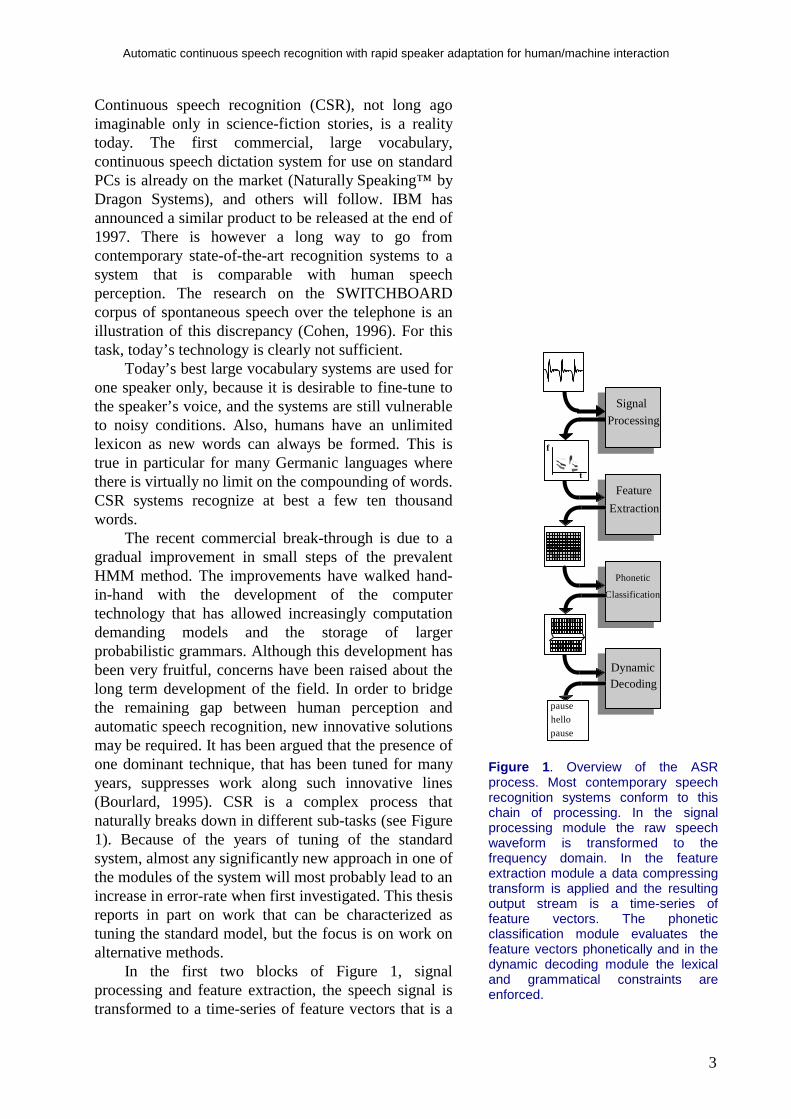
The recent commercial break-through is due to agradual improvement in small steps of the prevalentHMM method. The improvements have walked hand-in-hand with the development of the computertechnology that has allowed increasingly computationdemanding models and the storage of largerprobabilistic grammars. Although this development hasbeen very fruitful, concerns have been raised about thelong term development of the field. In order to bridgethe remaining gap between human perception andautomatic speech recognition, new innovative solutionsmay be required. It has been argued that the presence ofone dominant technique, that has been tuned for manyyears, suppresses work along such innovative lines(Bourlard, 1995). CSR is a complex process thatnaturally breaks down in different sub-tasks (see Figure1). Because of the years of tuning of the standardsystem, almost any significantly new approach in one ofthe modules of the system will most probably lead to anincrease in error-rate when first investigated. This thesisreports in part on work that can be characterized astuning the standard model, but the focus is on work onalternative methods.

In the first two blocks of Figure 1, signalprocessing and feature extraction, the speech signal istransformed to a time-series of feature vectors that is a

Signal

Processing

Feature

Extraction

Phonetic

Classification

DynamicDecoding

pausehello

pause

f

t

Figure 1 . Overview of the ASRprocess. Most contemporary speechrecognition systems conform to thischain of processing. In the signalprocessing module the raw speechwaveform is transformed to thefrequency domain. In the featureextraction module a data compressingtransform is applied and the resultingoutput stream is a time-series offeature vectors. The phoneticclassification module evaluates thefeature vectors phonetically and in thedynamic decoding module the lexicaland grammatical constraints areenforced.

Nikko Ström

4

suitable representation for the subsequent statisticalphonetic evaluation in the next module. The samplerate of the feature vectors is usually about 100 Hz.These first two blocks are often called the front-end ofthe ASR system. Apart from the implementation of afew of the most popular features, e.g., mel-frequencycepstrum coefficients, the work reported on in thisthesis is not much concerned with the front-end.

The standard method for implementing thephonetic classification module is to evaluate the featurevectors phonetically using multivariate Gaussianprobability density functions. The density functions areconditioned by the phoneme in context, i.e., theyestimate the likelihood of the feature vector given thehypothesized phoneme and its neighboring phonemes.However, several alternative methods have beenproposed. For example, Digalakis, Ostendorf andRohlicek (1992) use a stochastic model of phone-lengthsegments instead of evaluation of the feature vectorsindependently, and Glass, Chang, and McCandless(1996) use a method based on phone-length segmentfeature-vectors and discrete landmarks in the speechsignal.

Another alternative approach is the hybridHMM/ANN method (Bourlard and Wellekens, 1988),where an ANN is used for the phonetic evaluation ofthe feature vectors. The hybrid HMM/ANN method isused in Paper 3, Paper 5 and Paper 6 of this thesis andis discussed in more detail in the next section of thissummary.

The dynamic decoding module is where therecognition system searches for sequences of words thatmatch phoneme sequences with high likelihood in thephonetic evaluation. This is also the module where theprobabilistic grammar is included. Thus, wordsequences are evaluated on the merits of their phoneticmatch and their grammatical likelihood. The outputfrom the module is the most likely sequence of words,or a set of likely word sequence hypotheses that arethen further processed by other modules of the system.

The dynamic decoding search of a large vocabularyCSR system can be computationally very costly.Therefore, current research and development in thisfield are dominated by computational issues. Popularthemes for reducing computation are pruning and fastsearch. In pruning methods, partial hypotheses that arerelatively unlikely are not pursued in the continuedsearch. A particularly efficient pruning is proposed inPaper 3. In fast search methods, an initial fast, but less


5

accurate search is used to guide a subsequent, moreaccurate search, in order to pursue the most promisinghypotheses.

Multi-pass methods are generalizations of fastsearch. In a multi pass method, the output of the firstsearch pass is a set of the most likely hypotheses giventhe knowledge sources available in this first pass.Subsequent passes re-score the set of hypotheses basedon additional knowledge sources. The additionalknowledge sources require more computation, so it isbeneficial to apply them only on the selected set ofhypotheses instead of the whole search space. Examplesof knowledge sources that can be added in later passesare of the type that span word boundaries, e.g., higherorder N-grams in the probabilistic grammar, and tri-phones that condition on phones across wordboundaries.

A concept that can be applied to all the modules ofFigure 1 is speaker adaptation. Although the role ofspeaker adaptation in the human perception process isnot completely understood, there is convincingevidence that such a process takes place. In particular,the presence of a rapid adaptation was proposed byLadefoged and Broadbent (1957). This process operateson a time scale of a few syllables.

Speaker adaptation methods have beensuccessfully applied also for ASR. The success shouldbe no surprise, because of the discrepancy in theperformance between speaker-dependent (SD) andspeaker-independent (SI) systems (e.g., Huang and Lee,1991). Different adaptation methods can be classifiedby the amount of supervision required from the userand on what time-scale they operate. At one end of thespectrum are methods that require the user to read asample text that is then used to re-train the system. Thismethod can asymptotically reach the performance of acorresponding SD system if the size of the sample textis increased (e.g., Brown, Lee, and Spohrer, 1983;Gauvain and Lee, 1994). More advanced methodscollect the speaker-dependent sample as the system isrunning, and do re-training based on the data collected,without the need of a special training session by theuser. This latter scheme is called unsupervisedadaptation. However, both supervised and unsupervisedre-training methods are typically relatively slow – theadaptation effect is significant only after a minute ormore.

At the other end of the spectrum of speakeradaptation, are methods that have access to a model of

Nikko Ström

6

speaker variability. This additional knowledge lets thesystem concentrate on adapting to voices that are likelyto exist in the population of speakers, instead of blindlytrying to adapt based on the (initially) very smallsample from the new speaker. These methods can reacha positive adaptation effect after only a few syllables ofspeech. The speaker modeling approach to speakeradaptation is developed and investigated in the contextof hybrid HMM/ANN recognition in Paper 2, Paper 4and Paper 5. However, the approach does not require anANN model – a related adaptation scheme in the HMMdomain, is found in a paper by Leggeter and Woodland(1994), and Hazen and Glass (1997) use a relatedmethod in a segment-based system.

The remainder of this summary is organized insections corresponding to the three main directions ofwork: hybrid ANN/HMM recognition, dynamicdecoding, and fast speaker adaptation. The exception issection 4, that contains previously unpublished materialon the representation of large sets of alternativehypotheses – the output of the dynamic decodingsearch. Section 6 contains a brief presentation of theapplications of the developed CSR system. Finally,section 7 contains brief summaries and comments onthe included papers. In particular, the originalcontribution and innovative elements of each paper arediscussed in this section.


7

2. Hybrid HMM/ANN speech recognition

2.1 IntroductionThe continuous density hidden Markov model(CDHMM) is the dominant technology for automaticspeech recognition today. However, a few significantlimitations of the standard CDHMM suggest that othermethods, or combinations of CDHMM with othermethods, may improve the performance of therecognition. One class of such methods is based onartificial neural networks (ANNs).

Speech recognition was one of the first problemsthat ANN models were applied to during the rapidspread of the methods in the 1980’s. The complexmapping between the acoustic domain, and the set ofphonemes, has properties that are regarded to bemodeled well with ANN methods. One reason for thisis the good discriminative power of ANN models.

ANN models have been used for word recognitiondirectly (e.g., Ström, 1992; English and Boggess, 1992;Li, Naylor, and Rossen, 1992), but with limited success.It has been proven difficult to model the temporalaspects in an efficient manner within the ANNformalism. Combinations of an ANN with HMM thatmodels most of the temporal constraints have beenmore successful. Several different methods have beenproposed for combining the two. A few of the morewell-known are: “Hybrid HMM/ANN Architecture”(Bourlard and Wellekens, 1988), “Linked PredictiveNeural Networks” (Tebelskis and Waibel, 1990),“Hidden Control Neural Architecture” (Levin, 1990),and “Stochastic Observation HMM” (Mitchel, Harperand Jamieson, 1996).

The most successful architecture for combiningCDHMM and ANN technology is currently the hybridHMM/ANN model, where the ANN is utilized toestimate the observation probabilities of a CDHMM.This combination makes use of the discriminativepower of the ANN approach, and relies on the HMM tomodel temporal aspects and the invocation of aprobabilistic grammar.

In this chapter, the hybrid system used in several ofthe included papers is reviewed. First the CDHMM thatmodels the dynamic constrains imposed by the lexiconand grammar is discussed. Then I describe the ANNthat models the mapping between acoustic observations

Nikko Ström

8

and phonemes, and in section 2.5, sparse connectionand pruning in the ANN are covered.

2.2 The standard CDHMMAlthough used for speech recognition, the HMM ismost easily described as a speech production model. AnHMM based speech recognizer has a set of differentHMMs representing different units of speech, e.g.,phonemes or words. The recognition process is a searchto find the sequence of models that are the most likelyto have produced the utterance.

In the standard CDHMM formalism, the speechsignal is assumed to be produced by a probabilisticfinite state automaton (FSA). A graphic representationof an HMM, modeling a phoneme is shown in Figure 2.In the following I assume that all HMMs modelphonemes or special segments such as pauses etc. Themodel produces the signal by emitting, at each state ofthe FSA, an output observation and then moving to anew state. The emission of observations occurs atequidistant time-points, typically every 10 ms, and theoutput observation is a random variable with a differentprobability density function for each state. Also themotion between the states is governed by statisticallaws. The allowed transitions have transitionprobabilities associated with them such that some pathsthrough the FSA are more likely than others. This is theonly inherent duration modeling in the standardCDHMM.

The output probability densities are typicallymodeled by mixtures of multivariate Gaussianprobability distributions with diagonal covariancematrices. This functional form is selected mostly for itsmathematical properties, and in the case of the choiceof diagonal covariance matrices, to reducecomputations.

The observations are representations of the speechsignals in the short time frame of circa 10 ms coveredby each emission. A set of features, the feature vector,is computed for each frame. A popular basic featurevector is the so called cepstrum coefficients vector. Thecepstrum coefficients are the cosine coefficients of thespectrum of the signal in the frame. Typically, thecepstrum features, the total energy in the frame, and thefirst and second time-derivatives of these features, arethe components of the observation vectors modeled bythe multivariate mixture of Gaussian probabilitydistributions. The size of these observation vectors are

p11 p22 p33

p01 p12 p23 p34

ϕλ1(•) ϕλ2(•) ϕλ3(•)

{ } ( )( )

ϕπλ µ σ

µ

σ

=

−

=

=

= ⋅∑

=

=∑

∑w i

o

i

M

ii

M

i ij ij

ij ij

ijj

D

o wD

e

w

, ,

1

2

1

2

21 2

1

1

Figure 2 . Graphical representation ofan HMM. The HMM has one “hidden”stochastic process and one observablestochastic process. At each point intime, the model “is” in one of its states.The hidden process is the sequence ofstates visited. This process isgoverned by the transition probabilities,pij in the figure, for moving from onestate to another. The observableprocess is the output acoustic featurevector at each state. These vectors aremixtures of multivariate Gaussianstochastic variables (with densityfunction ϕ in the figure). This particularstructure with three states andtransitions from left to right, self-loopsbut no skips, is typically used forphoneme models.


9

typically around 40. The feature vector extraction isdiscussed in detail in Paper 3.

The framework of the CDHMM makes it straight-forward to optimize the model parameters using well-known parameter estimation paradigms from statistictheory. In particular, the maximum likelihood (ML)method is used. In short, it means that the parameters ofthe model – the means, variances and mixture weightsof the distributions, and the transition probabilities –should be chosen in such a way that the probability thatthe correct sequence of HMMs produced the utterancesof a training database is maximized. Or put in anotherway, the probability that the training utterances wereproduced by the models is maximized. There exists acomputationally efficient algorithm, the Baum-Welchalgorithm, that performs this maximization in aniterative expectation-maximization (EM) procedure.Each iteration of the algorithm is guaranteed to increasethe probability of the training utterances, and thusconvergence is established.

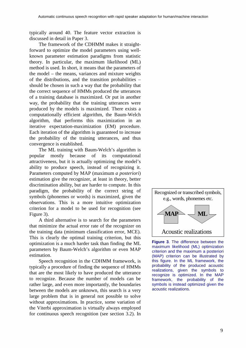
The ML training with Baum-Welch’s algorithm ispopular mostly because of its computationalattractiveness, but it is actually optimizing the model’sability to produce speech, instead of recognizing it.Parameters computed by MAP (maximum a posteriori)estimation give the recognizer, at least in theory, betterdiscrimination ability, but are harder to compute. In thisparadigm, the probability of the correct string ofsymbols (phonemes or words) is maximized, given theobservations. This is a more intuitive optimizationcriterion for a model to be used for recognition (seeFigure 3).

A third alternative is to search for the parametersthat minimize the actual error rate of the recognizer onthe training data (minimum classification error, MCE).This is clearly the optimal training criterion, but thisoptimization is a much harder task than finding the MLparameters by Baum-Welch’s algorithm or even MAPestimation.

Speech recognition in the CDHMM framework, istypically a procedure of finding the sequence of HMMsthat are the most likely to have produced the utteranceto recognize. Because the number of models can berather large, and even more importantly, the boundariesbetween the models are unknown, this search is a verylarge problem that is in general not possible to solvewithout approximations. In practice, some variation ofthe Viterbi approximation is virtually always employedfor continuous speech recognition (see section 3.2). In

Recognized or transcribed symbols,e.g., words, phonemes etc.

Acoustic realizations

MAP ML

Figure 3 . The difference between themaximum likelihood (ML) optimizationcriterion and the maximum a posteriori(MAP) criterion can be illustrated bythis figure. In the ML framework, theprobability of the produced acousticrealizations, given the symbols torecognize is optimized. In the MAPframework, the probability of thesymbols is instead optimized given theacoustic realizations.

Nikko Ström

10

this approximation it is assumed that the probability ofone path through the HMMs has much higherprobability than all other paths. It is very clear that thisunderlying assumption is often not justified, but onceagain it is the attractive computational properties of theso called Viterbi algorithm that has made it the standarddecoding method for CDHMM.

2.3 Problems with the standard modelThe weaknesses of the standard CDHMM model,touched upon in the previous section, have been pointedout by several authors (e.g., Bourlard and Morgan 1993;Robinson, 1994), and can be summarized in thefollowing points:1. Poor discrimination due to the fact that model

parameters are estimated by maximum likelihood(ML) estimation instead of an estimation methodthat attempts to explicitly minimize theclassification error. Examples of such estimationschemes are: minimum classification error (MCE),and maximum a posteriori (MAP) estimation.

2. The a priori choice of model topology, and inparticular the choice of functional form of thestatistical distributions, e.g., assuming that theemission probabilities for the acoustic observationsare mixtures of multivariate Gaussian densities withdiagonal covariance matrices. This choice is basedon the mathematical properties of the family ofdistribution functions and is not necessarily optimal.

3. The so called Markov assumption that statesequences are first-order Markov chains, i.e., theprobability density distributions depend only on thecurrent state.

4. The correlation between successive acousticobservations is not acknowledged. Note that this isdifferent from the previous point where theinfluence of the state sequence was considered.

5. There is a mismatch between the Baum-Welchtraining and evaluation of the HMMs because theViterbi approximation is active only in theevaluation phase.

Thus, it seems that we have a rather strong case againstthe HMM technology. However, during the history ofthe model, designers of state-of-the-art CDHMMrecognition systems have addressed all the above pointsand found ways to reduce the negative effects of them.The effects of point (3) have been reduced byintroducing context dependent models, e.g., tri-phones.


11

Point (4) has been addressed by adding delta and delta-delta coefficients to the observation vector. Parameter-tying schemes have made it possible to train verygeneral probability density functions that can solveproblems due to point (2), and recently, the ML trainingscheme has been complemented with MAP training inresponse to point (1).

To summarize the analysis of the weaknesses ofthe CDHMM: on the foundation of an initial model thatseems rather inappropriate for the task, an increasinglycomplex and more accurate model has emerged throughincremental refinement. It is noteworthy that theoriginal motivation for the choice of model that leads tothe discussed weaknesses was to keep computationdown, but the subsequent improvements that partiallysolved the initial problems have increased thecomputational demands dramatically. This is true inparticular for the many models needed for triphonemodeling and the computationally demandingprobability distribution functions used. Thus, theimprovements go hand in hand with the rapiddevelopment of computers.

Given the above, it is not self-evident that theCDHMM would be the choice of model if automaticspeech recognition were to be reinvented today. Butbecause of the complexity of the problem and the largeresearch and development investments in the currenttechnology, it is very difficult to make a competitivesystem based on a completely new framework. WhenBourlard (1995) discusses the present situation in theASR field, he characterizes the prevailing CDHMMarchitecture as a local optimum in the space ofrecognition systems. He argues that it is necessary tochange the architecture in a manner that increasesrecognition error rates in the short run, but has potentialof long term improvement, thus escaping from the localoptimum.

In the hybrid HMM/ANN architecture, thestandard framework is kept intact, but the observationprobabilities are computed by an ANN. This addressespoint (1) and (2) above, by the selection of model andtraining paradigm chosen – ANNs put very weak apriori constraints on the distributions and are trained inthe MAP paradigm. Point (5) is also neutralizedbecause the Baum-Welch algorithm is not used, butmany of the imperfections of the standard modelremain, e.g., the Viterbi approximation and points (3)and (4).

Nikko Ström

12

2.4 The artificial neural networkIn the late 1980’s it was pointed out by several authorsthat the output activities of ANNs trained with theback-propagation algorithm approximate the aposteriori class probabilities (Baum and Wilczek 1988;Bourlard and Wellekens, 1988; Gish, 1990; Richardand Lippman, 1991). In the case of an ANN trained torecognize phonemes, this means that the ANNestimates the probability of each phoneme given theacoustic observation vector. This observation is offundamental importance for the theoretical justificationof the hybrid HMM/ANN model. By application ofBayes’ rule, it is easy to convert the a posterioriprobabilities to observation likelihoods, i.e,

( ) ( )( ) ( )p o c

p c o

p cp oi

i

i

||

=(1)

where ci is the event that phoneme i is the correctphoneme, o is the acoustic observation, and p(ci) is thea priori likelihood of phoneme i. The unconditionedobservation probability, p(o), is a constant for allphonemes and can consequently be dropped withoutchanging the relative relation between phonemes, andthe a priori phoneme probabilities are easily computedfrom relative frequencies in training speech data. Thus,equation (1) can be used to define output probabilitydensity functions of a CDHMM.

Back-propagation ANNs have intrinsically manyof the features that have been added to the standardCDHMM in the development process discussed in theprevious section. The normal back-propagationestimates MAP phoneme probabilities, not MLestimates that is the normal estimation method forCDHMM. As mentioned, MAP has betterdiscrimination ability than ML, and is a more intuitivemethod to train a model for recognition.


13

Also the parameter sharing/tying is available in theANN at no extra cost. This was introduced in theCDHMM with added complexity as a consequence, tobe able to use complex probability density functionswithout introducing too many free parameters. In Figure4 it is seen that all output-units in the ANN share theintermediate results computed in the hidden units.However, this total sharing scheme can sometimes hurtperformance and it is therefore beneficial to limit thesharing of hidden units. This is discussed more insection 2.5.

The important short time dynamic features –formant transitions etc. – have been captured in ANNsby time-delayed connections between units (Waibel etal., 1987). This is a more general mechanism than thesimple dynamic features (1st and 2nd time-derivatives)used in the standard CDHMM. One use of time-delayedconnections is to let hidden units merge informationfrom a window of acoustic observations, e.g., a numberof frames centered at the frame to evaluate. The samemechanism can be used to feed the activity of thehidden units at past times, e.g., the previous time point,back to the hidden units. This yields recurrent networksthat utilize contextual information by their internalmemory in the hidden units (e.g., Robinson andFallside, 1991). A general ANN architecture thatencompasses both time delay windows and recurrency,is presented in Paper 6.

Problems that are related to the HMM-part of thehybrid, are of course not solved by the introduction ofthe ANN. The Markov assumption, the Viterbiapproximation etc. still remain. In many cases, the adhoc solutions developed to reduce the effects of theseproblems for CDHMM can easily be translated to thehybrid environment, but in the case of contextdependent models, e.g., tri-phones, there is an extracomplication. It is not as straight-forward to applyBayes’ rule to the output activities when they areconditioned by the surrounding phoneme identities. Itturns out that, to compute the observation likelihood inthis case, the probability of the context given theobservation is needed, i.e.,

( ) ( ) ( )( )

( ) ( ) ( )( ) ( )

p o l c rp c l r o p o l r

p c l r

p c l r o p l r o p o

p c l r p l r

| , ,| , , | ,

| ,

| , , , |

| , ,

= =(2)

hiddenunits

input units

output units

a1 a2

a6a5

a3 a4

a7 a8 a9 a10

a11 a13a12 a14

( ) ( )

( )a w a x

e

a w a w a w a w a

i ji jj

n

xi= =

+= + + +

= −∑σ σ

σ

1

5 15 1 25 2 35 45 4

1

1

3

,

e.g.,

Figure 4 . Graphical representation ofa feed-forward ANN. Associated witheach node at each time is an activity.This is a real bounded number, e.g.,[0; 1] or [-1; 1]. The activities of theinput units constitutes the input patternto classify. The activities of all otherunits are computed by taking aweighted sum of the activities of theunits in lower layers, and then applyinga compressing function σ to get abounded value. The activities of theoutput units are the network responseto the input pattern. To train an ANNfor a particular task, a trainingdatabase is prepared with inputpatterns and corresponding targetvectors for the output units. Theweights, wij, of the ANN are adjusted tomake the output units’ activities asclose as possible to the target values.This is done iteratively in the so calledback-propagation training.

Nikko Ström

14

where c is the phoneme, and l and r are the right andleft context phonemes. This problem has been solvedby (Bourlard and Morgan, 1993; Kershaw, Hochbergand Robinson, 1996) by introducing a separate set ofoutput units for the context probabilities, p(l,r |o), buttheir results indicate that the gain with tri-phones issmaller for the hybrid model than for the standardCDHMM.

2.5 Sparse connectivity and pruning in theANN

The number of hidden units determines to a large extenta network’s ability to estimate the a posterioriprobabilities accurately. One could argue that it is thenumber of free trainable parameters in the network thatis the important factor. In this view, it is not the numberof units, but the number of connections that isimportant. However, from experience we know that notonly the number of parameters is important, but alsohow they are put to use. In large, fully-connectednetworks, the number of connections is several ordersof magnitude higher than the number of units. Thismeans that each unit has several hundred, sometimesthousands of in-flowing connections. It is unlikely thatall these connections can provide useful information tothe one-dimensional output of the unit. Also, bystudying the distribution of the weights in trainedANNs it can be noted that there is a high concentrationof weights close to zero. Therefore it can beadvantageous to work with sparsely connectednetworks where units are connected only to a fraction ofall units in higher layers.

In Paper 6 I show that the ANN performance canbe greatly increased by shifting the balance between thenumber of units and connections by introducing sparseconnectivity. Two different approaches for achievingsparse connectivity are explored: connection pruningand sparse connection.

Connection pruning is a method that is appliedafter the network is trained. The network is analyzedand each connection is given a measure of salience. Afraction of the connections with the smallest salience isthen removed and the resulting, smaller ANN isretrained. The most well-known pruning criterion is dueto Le Cun, Denker, and Solla (1990), and was given theimaginative name “Optimal Brain Damage”. In thismethod the salience depends on the second derivativeof the objective function of the back-propagation. In


15

Paper 6, a more simplistic measure is used, the salienceis simply the magnitude of the connection weight.

In Paper 6, a reduction to about half the number ofconnections was found to be possible withoutsignificant performance degradation. Thecomputational complexity for running the ANN isproportional to the number of connections. Thus, thismay be of great importance when computation iscritical. Since pruning reduces the number of freeparameters, it can also improve the network’sgeneralization ability (e.g. Le Cun, Denker and Solla,1990; Sietsma and Dow, 1991), but since we used atruncated training that handles problems with over-adaptation to the training data, this potential benefit isless important in our case.

Pruning the connections of an already trainednetwork has no impact on the computational effort fortraining. To be able to apply the pruning criterion to theconnections, the weights of the fully connected networkmust first be trained. Therefore, a second method – tostart the training with already sparsely connectednetworks – was also explored in Paper 6. Beforetraining, there is no available information about whichconnections are salient, so a random set of connectionsmust be selected. Of course, this is in general not anoptimal set, but the results show that sparsely connectedANNs perform much better than their fully connectedcounterparts with equal number of connections.

Nikko Ström

16

3. Dynamic Decoding

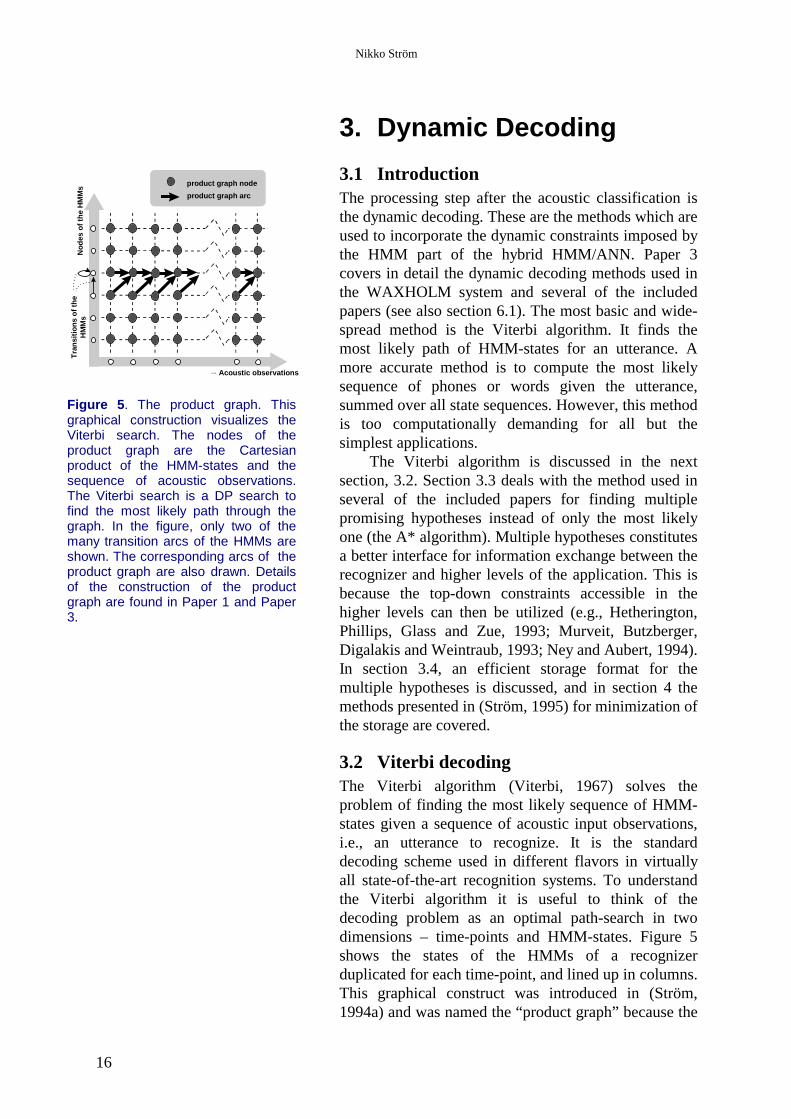
3.1 IntroductionThe processing step after the acoustic classification isthe dynamic decoding. These are the methods which areused to incorporate the dynamic constraints imposed bythe HMM part of the hybrid HMM/ANN. Paper 3covers in detail the dynamic decoding methods used inthe WAXHOLM system and several of the includedpapers (see also section 6.1). The most basic and wide-spread method is the Viterbi algorithm. It finds themost likely path of HMM-states for an utterance. Amore accurate method is to compute the most likelysequence of phones or words given the utterance,summed over all state sequences. However, this methodis too computationally demanding for all but thesimplest applications.

The Viterbi algorithm is discussed in the nextsection, 3.2. Section 3.3 deals with the method used inseveral of the included papers for finding multiplepromising hypotheses instead of only the most likelyone (the A* algorithm). Multiple hypotheses constitutesa better interface for information exchange between therecognizer and higher levels of the application. This isbecause the top-down constraints accessible in thehigher levels can then be utilized (e.g., Hetherington,Phillips, Glass and Zue, 1993; Murveit, Butzberger,Digalakis and Weintraub, 1993; Ney and Aubert, 1994).In section 3.4, an efficient storage format for themultiple hypotheses is discussed, and in section 4 themethods presented in (Ström, 1995) for minimization ofthe storage are covered.

3.2 Viterbi decodingThe Viterbi algorithm (Viterbi, 1967) solves theproblem of finding the most likely sequence of HMM-states given a sequence of acoustic input observations,i.e., an utterance to recognize. It is the standarddecoding scheme used in different flavors in virtuallyall state-of-the-art recognition systems. To understandthe Viterbi algorithm it is useful to think of thedecoding problem as an optimal path-search in twodimensions – time-points and HMM-states. Figure 5shows the states of the HMMs of a recognizerduplicated for each time-point, and lined up in columns.This graphical construct was introduced in (Ström,1994a) and was named the “product graph” because the

Nod

es o

f the

HM

Ms

Tra

nsiti

ons

of th

eH

MM

s

Acoustic observations

product graph node

product graph arc

...

Figure 5 . The product graph. Thisgraphical construction visualizes theViterbi search. The nodes of theproduct graph are the Cartesianproduct of the HMM-states and thesequence of acoustic observations.The Viterbi search is a DP search tofind the most likely path through thegraph. In the figure, only two of themany transition arcs of the HMMs areshown. The corresponding arcs of theproduct graph are also drawn. Detailsof the construction of the productgraph are found in Paper 1 and Paper3.


17

nodes are the Cartesian product of the nodes of theHMMs and the time-points.

In Paper 3, I account in detail for how the best pathis found in the 2-dimensional grid of Figure 5. Thegeneral principle is dynamic programming (DP), whichyields a time-synchronous search, i.e., time-points areprocessed one at a time. Therefore the search can beperformed in real time as the speaker utters a sentence.This is an important feature in human/machine dialoguewhere short response times often are critical for users’acceptance of the systems.

The Viterbi search is the most computationallydemanding part of the dynamic decoding of the systemdescribed in Paper 3, but several approximations areused to keep computation down. The most importantone is beam pruning. A combination of two differentpruning criteria – both a threshold on the pathprobabilities and a maximum number of alive paths –are enforced. A section of Paper 3 is devoted to thistopic that is of great importance for fast computation. Itis shown that the combination of the pruning criteria ismore efficient than each criterion by itself.

3.3 The N-best paradigm and A* searchA human/machine dialogue system is a large andcomplex software program that is impossible toconstruct and maintain without a great deal ofmodularity. For example, the ASR module takes audiospeech input and delivers a symbolic representation ofthe utterance as its output. Interpretation of the meaningof the utterance is left to higher level modules. Thesymbolic representation can simply consist of the mostlikely string of words computed by the Viterbialgorithm. However, because the ASR module does notnecessarily have access to information about the currentdialogue state, or a deep syntactic, semantic andpragmatic analysis of the utterance, this is probably notthe optimal interface to other modules.

An output representation that takes betteradvantage of the acoustic evidence is one where theASR module delivers a set of acoustically scoredhypotheses to higher modules. These modules can thenselect the most likely word-string hypothesis on thebasis of both the acoustical evidence computed by theASR module, and the syntactic, semantic and pragmaticanalysis. A popular representation of this set ofhypotheses is an N-best list. This is simply a list of theN most likely word strings given the sequence ofacoustic observation vectors. Thus, an N-best list is a

waxholmfor

four

leave

leave

boatthe

does

as

giveboat

boat

time

next nodeto expand

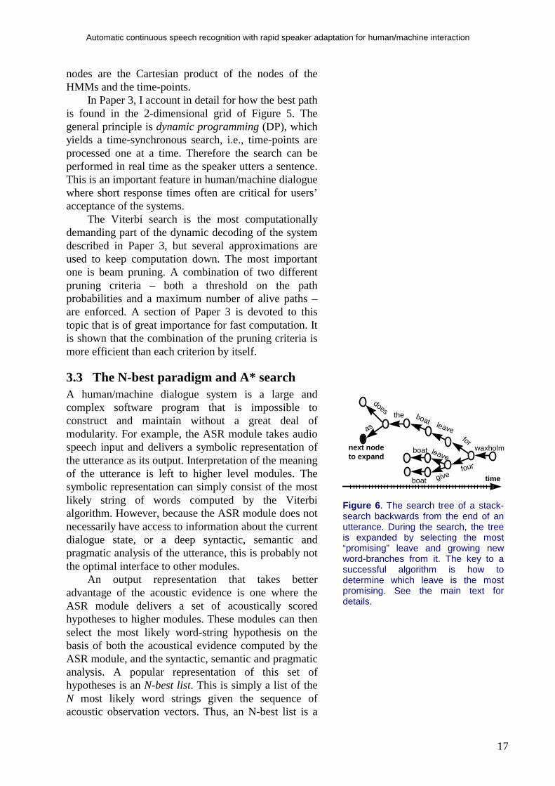
Figure 6 . The search tree of a stack-search backwards from the end of anutterance. During the search, the treeis expanded by selecting the most“promising” leave and growing newword-branches from it. The key to asuccessful algorithm is how todetermine which leave is the mostpromising. See the main text fordetails.

Nikko Ström

18

generalization of the output of the Viterbi algorithm (inthe case of the Viterbi algorithm, N = 1).

Finding the N-best word-strings is a significantlyharder problem than just finding the most likely word-string. It can be solved by extending the DP search andkeeping a stack of hypotheses at each search point inFigure 5 instead of just the most likely as in thestandard Viterbi algorithm. This has the advantage ofpreserving the time-synchronous feature of the Viterbialgorithm, but the complexity is proportional to N, i.e.,the already computationally demanding algorithmbecomes slower in proportion to the desired number ofhypotheses.

A more computationally efficient method is the socalled A* (a-star) search. This method is based on thestack decoding paradigm where a search tree is builtwith partial hypotheses represented by paths from theroot to the leaves. The word-symbols are associatedwith the branches of the tree (see Figure 6). During thesearch, most paths are partial hypotheses, i.e., they donot cover the whole utterance. The partial path that ismost promising according to a search heuristic isexpanded by growing new branches from its leave.When there are enough complete paths in the tree, thesearch is terminated.

The key to an efficient A* search is the searchheuristic. When evaluating partial paths, the likelihoodof the words in the path so far, given the acousticobservation, is easily accessible and should of course beutilized. But it turns out that this is not enough – it isalso necessary to estimate the influence of theremainder of the utterance. It is possible that a partialpath with a high likelihood turns out to be in a “dead-end”, and can not be completed with a high likelihood.

It was an observation of Soong and Huang (1991)that made A* practically applicable to the N-bestproblem in ASR. They realized that the likelihoodscomputed in the Viterbi algorithm constitute aparticularly well behaved A* heuristic. In the Viterbisearch, the highest likelihoods of the observations fromthe beginning of the utterance to all points in theproduct graph (see Figure 5) are computed. If the A*search is performed backwards from the end of theutterance, the partial paths are from some interior pointto the end of the utterance, and the remainder of theutterance is from the beginning to the interior point.Thus, the best possible likelihood for the remainder ofthe utterance is the likelihood computed in the Viterbisearch. This particular heuristic has many attractive


19

features, one is that complete paths are expanded inorder of likelihood, i.e., when N complete paths withdifferent word strings have been expanded, the searchcan be terminated.

The development of an A* search algorithm,currently used in the WAXHOLM dialogue system hasbeen a significant part of my work in the ASR field, andis reported on in Paper 1 and Paper 3. The most originalaspect of the work in this area is the optimization of the“lexical network”, introduced in Paper 1, that greatlyreduces computation in the search. The optimizationmethod is developed further in Paper 3, where theconcept of word pivot arcs is introduced. Although inthis case it is used only in the A* framework, wordpivot arcs are relevant also in standard Viterbidecoding, because they can be used to significantlyreduce the size of the product graph.

3.4 Word lattice representation of multiplehypotheses

Passing N-best lists from the ASR module as therecognition result to higher level modules is a step thatincreases the coupling between the modules withoutdecreasing the modularity. It is a clean interfacebetween modules, but in some cases the entry in the N-best list that is optimal after considering knowledgesources provided by higher level modules, is very fardown the list. Thus, it is necessary to pass long listsbetween the modules. In this case, a so called word-lattice or word-graph is a better representation of thehypotheses because it is more compact (see Figure 7and Figure 8).

In Paper 3, the A* search is modified to produce aword-lattice instead of an N-best list. A word lattice is agraph that generates all hypotheses, including all time-alignments of the words, above a likelihood threshold.This is the method now used in the WAXHOLMdemonstration system (see section 6.1). The dialoguemodule of the WAXHOLM system requires an N-bestlist as input, but this is computed in a subsequent searchin the word-lattice.

The direct construction of a word-lattice in the A*search gives a cleaner implementation, but alsoimproves the performance. It is computationallyadvantageous to make a separate search for the N-besthypotheses in the produced word-lattice instead ofproducing the list while performing the first A* search.The reason is that finding the N-best list is inherently an

Vaxholmthe boatwhen

does

as

leave

give

four

for

when as the boat give for Vaxholm when does the boat give for Vaxholmwhen as the boat leave for Vaxholmwhen does the boat leave for Vaxholmwhen as the boat give four Vaxholmwhen does the boat give four Vaxholmwhen as the boat leave four Vaxholmwhen does the boat leave four Vaxholm

Word graph

N-best list

Figure 7 . Two differentrepresentations of a set of hypotheses.From this simple example, thedifference between the two formats isclearly seen. The entries in the N-bestlist are typically similar to each other,therefore it is sometimes practical towork with the more compact wordgraph representation.

0 100 200 300 400 500100

101

102

103

104

105

word lattice density

size of equivalent N-best list

Figure 8 . This graph shows the size ofthe word lattice (number of arcs perword) versus the number of entries inan hypothetical N-best list covering thesame hypotheses. It is easy to see thebenefit of the word lattice for large setsof hypotheses. The example is takenfrom Paper 3.

Nikko Ström

20

exponential complexity problem while constructing theword-lattice is of polynomial complexity (this isdiscussed in Paper 3).


21

4. Word graph minimizationThis section is an extended version of the summary (Ström, 1995) of a presentation at theIEEE Workshop on Automatic Speech Recognition, 1995. This extended material has not beenpublished before.

4.1 IntroductionWith the development of complex speech technologyapplications, the ability of an automatic speechrecognition (ASR) system to output multiplerecognition hypotheses is becoming increasinglyimportant. Examples of such applications arehuman/dialogue applications and machine translationwhere the ASR must interact with modules that handlediscourse, semantics and pragmatics. Passing multiplerecognition hypotheses to the higher levels of thesystem is a way of increasing the coupling withoutdecreasing the modularity, which is essential for thedevelopment of large complex systems.

Another use is hypothesis re-scoring, where themultiple hypotheses are an internal, intermediaterepresentation generated by a fast initial search. Theseare then used to limit the search-space in a second,more accurate search.

Word-lattices and word-graphs provide a compactrepresentation of sets of hypotheses as described insection 3.4. I will mean by a word-lattice, a word graphthat contains all time alignments that have a likelihoodabove the pruning threshold.

For re-scoring using new acoustic models, theword-lattice constructed in the A* search is a goodrepresentation because in this case, it is necessary to re-score the different alignments. However, if theobjective is re-scoring using only a new grammar, themultiple time-alignments are excessive, and a morecompact representation is better.

4.2 Problem formulationIt is not trivial to define a measure of size for word-graphs. From a practical point of view, the size of thegraph should reflect the amount of computationrequired to perform critical operations on the graph.Such an operation may for example be searching for themost likely path through the graph. The number of arcsis in many cases a good indication on the amount ofcomputation required, and a wide-spread measure ofword-graph size is lattice density. The lattice density ofa word-graph is the number of arcs divided by the

Nikko Ström

22

number of words actually uttered (Ney and Aubert,1994).

Another measure of size is the number of nodes inthe graph. In contrast to the number of arcs, the numberof nodes has typically only a small impact on thecomputation required for search operations. Instead thememory requirement of the algorithms is affectedbecause search algorithms often store state-informationfor the nodes at each time-frame.

If the objective is re-scoring word-graphs with anew grammar, the time-alignments of words is notimportant and it is therefore desirable to reduce the sizeas much as possible without altering the generated setof word-strings. Thus, the problem can be defined asfinding the word-graph with the minimum number ofarcs or nodes that generates exactly the same word-strings as a given word-lattice.

4.3 Approximative methodsA word lattice is a directed acyclic graph (DAG) – asubclass of non-deterministic finite state automatons(NFA) (see for example Hopcroft and Ullman, 1979).Minimizing an NFA is a hard problem that can not ingeneral be solved in polynomial time. Therefore, theproblem has been attacked using heuristic methods thatreduce the graph but not to its minimal size.

In the word-pair approximation (Ney and Aubert,1994), it is assumed that the positions of wordboundaries are independent. In most cases this is asound assumption, but it may lead to search errors forshort words and when a minimum duration constraint isenforced for phones.

In the A* search by Hetherington, Phillips, Glassand Zue (1993), arcs are not added to a node of theword-graph if they do not introduce a new partial word-sequence. This reduces the constructed graphsignificantly.

4.4 The minimal deterministic graphAlthough the approximate methods can be quiteeffective, it is not satisfactory to settle with anapproximation without having established a baselinewith an exact method.

A well-known minimization algorithm exists forminimizing NFAs. The procedure results in a minimal(with respect to the number of nodes) equivalentdeterministic finite automaton (DFA). This is a welldefined objective, and in addition the deterministic

0 100 200 300 400 5001

2

3

4

5

6

7

word lattice density

density of minimaldeterministic graph

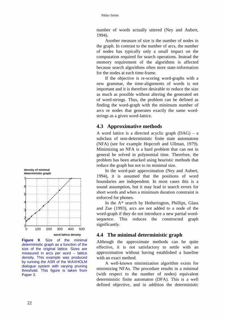
Figure 9 . Size of the minimaldeterministic graph as a function of thesize of the original lattice. Sizes aremeasured in arcs per word – latticedensity. This example was producedby running the ASR of the WAXHOLMdialogue system with varying pruningthreshold. This figure is taken fromPaper 3.


23

property of the resulting graphs has some other niceeffects.

The algorithm (Hopcroft and Ullman, 1979) can bebroken down into two steps. The first step is toconstruct an equivalent deterministic finite stateautomaton (DFA) – the “determinization”. Adeterministic FSA has the property that, given asequence of words, there is at most one path throughthe graph that generates it. This is accomplished forexample by allowing only one start state and no morethan one out-flowing arc for each word from any state.The second step is minimization of the DFA to obtainthe minimal deterministic graph – the minimization.

The resulting reduction of the number ofconnections in the graph can be seen in Figure 9. In thisexample the reduction is about 50 times, but this islikely to be a problem dependent number.

Of the two steps, the determinization is thecomputationally hardest. In general the determinizationcan not be done in polynomial time or space. But as wewill see, the particular structure of word-graphs can beutilized to attain an acceptable computational cost. Theminimization algorithm has N log(N) complexity ingeneral, but in the case of word-graphs this can bereduced to approximately linear complexity. In the nexttwo sections the two steps are reviewed briefly. A morethorough account of the classic algorithm can be foundin (Hopcroft and Ullman, 1979). Here we focus on theaspects that are specific to optimizing word-graphs –the short-cuts due to the special structure of word-graphs, and computational considerations given thisparticular type of NFA.

4.5 DeterminizationThe key to the determinization algorithm is theidentification of sets of nodes in the original graph withsingle nodes in the resulting deterministic graph. This isalso what causes the exponential computationalcomplexity as there are 2N sets of nodes in an originalgraph of N nodes. Fortunately, all sets will not beconsidered during the construction of the deterministicgraph. Still, the main effort in the implementation ofthe algorithm involves the storage of sets of nodes in anefficient manner.

To simplify the algorithm slightly, we assume thatthere is exactly one start node and one end node in thegraph. This can easily be enforced in the case of word-lattices, in particular if all utterances must begin andend with the special “silence” symbol.

ss

s

ss s

ss

a bc

b

c

c de

d

dd

ed

gg

h

g ff

f ff

i

Original, non-deterministic lattice

Deterministic graph

nendn0

s ic

h

gs

f

f

b ss

d

b

ade

e

ss

s

ss

sss

ab

cb

c

c de

d

d dd

gg

h

g ff

f ff

i

Nend

Sets of nodes for construction of deterministic graph

N0

e

Figure 10 . Illustration of thedeterminization algorithm described inthe main text. The set N0 is the first tobe taken care of in step 4, and thereare only words labeled “s” flowing outfrom it so w=s. The set of nodesreached by the s-arcs is the next nodeof the deterministic graph. This set inturn has four different words flowingout from it (c, i, g, h), and fourcorresponding new sets are formed.The process continues until no newsets are formed.

Nikko Ström

24

The algorithm can now be described as follows:1) Identify nodes ni of the deterministic graph with sets

of nodes Ni in the original latice.2) Define N0 to be the set containing only the start

node of the lattice, and Nend to be the set containingonly the end node of the lattice.

3) Initialize the deterministic graph with the node n0.4) For each node, nx in the deterministic graph and

each word wLet Ny be the set of nodes in the lattice thatcan be reached from a node in Nx with theword w.

If there is no node ny in the deterministicgraph - add it.

Add an arc with word w from nx to ny.

The procedure is illustrated in Figure 10.Computationally, the greatest problem is how to

store the sets of nodes in an efficient manner. It isimportant to be able to quickly determine whether a setalready exists, or if it represents a new node in thedeterministic graph. In the implementation, this wassolved by a combination of a hash-table and comparingsorted sets of nodes. The hash table is based on a hash-key that is independent of the order of the nodes, andthe sets are not sorted unless necessary. This means thatwhenever an already existing set is looked up, it will benecessary to sort it and the lists with the same hash-keyamong the already existing. But no sorting is needed toinsert a new set unless a hash-table clash occurs.Because large sets are likely to be looked up only once,the effect is that larger sets are seldom sorted.

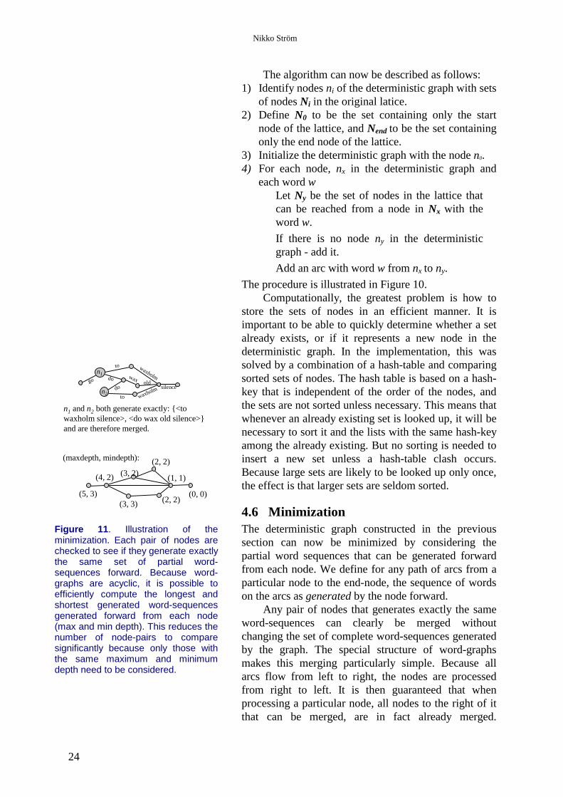
4.6 MinimizationThe deterministic graph constructed in the previoussection can now be minimized by considering thepartial word sequences that can be generated forwardfrom each node. We define for any path of arcs from aparticular node to the end-node, the sequence of wordson the arcs as generated by the node forward.

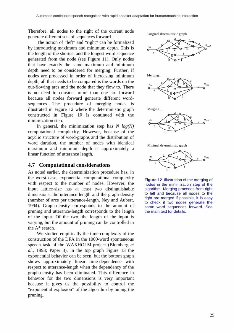
Any pair of nodes that generates exactly the sameword-sequences can clearly be merged withoutchanging the set of complete word-sequences generatedby the graph. The special structure of word-graphsmakes this merging particularly simple. Because allarcs flow from left to right, the nodes are processedfrom right to left. It is then guaranteed that whenprocessing a particular node, all nodes to the right of itthat can be merged, are in fact already merged.

silence

n1

n2

go

to waxholm

do

do

to waxholm

wax old

n1 and n2 both generate exactly: {<towaxholm silence>, <do wax old silence>}and are therefore merged.

(maxdepth, mindepth):

(0, 0)

(4, 2) (3, 2)

(3, 3)

(2, 2)

(1, 1)

(2, 2)(5, 3)

Figure 11 . Illustration of theminimization. Each pair of nodes arechecked to see if they generate exactlythe same set of partial word-sequences forward. Because word-graphs are acyclic, it is possible toefficiently compute the longest andshortest generated word-sequencesgenerated forward from each node(max and min depth). This reduces thenumber of node-pairs to comparesignificantly because only those withthe same maximum and minimumdepth need to be considered.


25

Therefore, all nodes to the right of the current nodegenerate different sets of sequences forward.

The notion of “left” and “right” can be formalizedby introducing maximum and minimum depth. This isthe length of the shortest and the longest word sequencegenerated from the node (see Figure 11). Only nodesthat have exactly the same maximum and minimumdepth need to be considered for merging. Further, ifnodes are processed in order of increasing minimumdepth, all that needs to be compared is the words on theout-flowing arcs and the node that they flow to. Thereis no need to consider more than one arc forwardbecause all nodes forward generate different word-sequences. The procedure of merging nodes isillustrated in Figure 12 where the deterministic graphconstructed in Figure 10 is continued with theminimization step.

In general, the minimization step has N log(N)computational complexity. However, because of theacyclic structure of word-graphs and the distribution ofword duration, the number of nodes with identicalmaximum and minimum depth is approximately alinear function of utterance length.

4.7 Computational considerationsAs noted earlier, the determinization procedure has, inthe worst case, exponential computational complexitywith respect to the number of nodes. However, theinput lattice-size has at least two distinguishabledimensions: the utterance-length and the graph-density(number of arcs per utterance-length, Ney and Aubert,1994). Graph-density corresponds to the amount ofpruning and utterance-length corresponds to the lengthof the input. Of the two, the length of the input isvarying, but the amount of pruning can be controlled inthe A* search.

We studied empirically the time-complexity of theconstruction of the DFA in the 1000-word spontaneousspeech task of the WAXHOLM-project (Blomberg etal., 1993; Paper 3). In the top graph Figure 13 theexponential behavior can be seen, but the bottom graphshows approximately linear time-dependence withrespect to utterance-length when the dependency of thegraph-density has been eliminated. This difference inbehavior for the two dimensions is very importantbecause it gives us the possibility to control the“exponential explosion” of the algorithm by tuning thepruning.

nendn0

si

c

h

gf

b sb

ade

Minimal deterministic graph

Original deterministic graph

nendn0

si

c

hg

s

f

f

b s

s

d

b

ad

ee

Merging...

nendn0

s i

c

hg

ff

bs

d

b

ade

e

nendn0

s

ic

h

gf

bs

d

b

ade

e

Merging...

Figure 12 . Illustration of the merging ofnodes in the minimization step of thealgorithm. Merging proceeds from rightto left and because all nodes to theright are merged if possible, it is easyto check if two nodes generate thesame word sequences forward. Seethe main text for details.

Nikko Ström

26

For comparison, the word-pair approximation wasalso investigated. Applying the word-pairapproximation to the word-lattice resulted on average ina reduction in the number of arcs to 8.1% of theoriginal lattice. The minimal deterministic graph for thesame word-lattice was on average reduced to 1.4% ofthe lattice.

4.8 DiscussionThe exact minimization algorithm investigated in thisstudy was clearly shown to produce smaller graphs thanthe approximate word-pair approximation method. Thisis true in spite of the fact that the exact algorithmminimizes the number of nodes, but the two methodsare compared on the basis of the number of arcs. In theexample investigated, the exact algorithm producedalmost six times smaller graphs than the approximatemethod, but the exact quotient is likely to be dependenton the lexicon, pruning aggressiveness etc.

In contrast to the word-pair approximation, thegraph of the proposed algorithm generates exactly thesame word-strings as the original lattice (no hypothesesare lost by approximation). However, since theproposed method is exponential with respect to lattice-density, a hybrid-approach where the lattice is firstreduced by the word-pair approximation and thenminimized, seems to be an attractive alternative.

The computational demands of the exactminimization are probably too high for use in the on-line recognition mode of a real-time ASR system (withcontemporary computer technology). However, for off-line tasks, where the same minimized word-graphs areused repeatedly, the effort may be worthwhile. Iterativeestimation of grammar parameters during training ofthe system is one example.

com

pu

tatio

n ti

me

[s]

com

p.

time

/ e

xp(a

rcs/

wo

rd)

lattice density [arcs/word]

number of words

Figure 13. Top: Time for constructionof the DFA as a function of the lattice-density.Bottom: Construction timedivided by the exponential of the latticedensity. The simulation was made on aSPARC 10 workstation.


27

5. Speaker adaptation

5.1 IntroductionSpeaker adaptation is one of the main areas of work ofthis thesis. In particular, rapid adaptation to a new voicehas been investigated. Although there is evidence forsuch an adaptation process in speech perception, therole of speaker adaptation in the speech perceptionprocess is still not completely understood. In a famousexperiment with synthetic speech stimuli, Ladefogedand Broadbent (1957) found that altering the formantfrequencies in a precursor utterance resulted indifferently perceived identity of a target word. Toaccount for this effect they postulated a psychologicaladaptation process and concluded that:

“... unknown vowels are identified in termsof the way in which their acoustic structurefits into the pattern of sounds that the listenerhas been able to observe.”

This view has been very influential, but it has beenchallenged by others arguing that the effect is of minorimportance in the perception of natural speech. Inparticular, the dynamic patterns of the vowels in theirconsonantal context have been ascribed moreimportance (Verbrugge and Strange 1976, Strange1989). Strange (1989) wrote:

“If, as perceptual results suggest, there issufficient information within single syllablesto allow the listener to identify intendedvowels, even when those vowels arecoarticulated by different speakers indifferent consonantal contexts, then the needto postulate psychological processes bywhich the perceiver enriches otherwiseambiguous sensory input is eliminated.”

In ASR, the performance gap between speaker-independent (SI) and speaker dependent (SD) systems(e.g., Huang and Lee 1991) indicates that there is a lotto be gained from adapting SI-models to the speaker.Certainly, the variation due to consonantal context isrecognized as an important property of the speech-signal also for ASR. This is usually modeled by contextdependent models, e.g., triphones. Nevertheless, thereis general agreement that speaker adaptation schemescan further improve recognition performance

Nikko Ström

28

significantly. An overview of existing methods forspeaker adaptation in ASR is given in Paper 4.

Paper 2, Paper 4 and Paper 5 represent a line ofwork that aims at performing rapid speaker adaptationby accessing knowledge from an explicit model of thespeaker variability. The idea is that a priori knowledgeof the speaker variability will reduce the amount ofadaptation data necessary from the new speaker byconstraining the parameter space. For example, thevariability due to varying vocal tract length affects theformant patterns of all voiced phones in a coherent andsystematic fashion. Thus, if the rules governing thisvariability are known, it is not necessary to collectadaptation data for all phonemes.

Key concepts of the framework of Paper 2, Paper 4and Paper 5 are the speaker model that models thespeaker variability, and the speaker space that is thedomain of a set of parameters describing different voicecharacteristics. A speaker model is basically aprobability distribution function over a speaker space.

5.2 Speaker modelingA speaker model is a statistical model of the speakervariability. It includes a parametric description of thevariability and an a priori probability distribution forthe different characteristics. For example, vocal-tractlength is a characteristic that can be of importance in aspeaker model, independent of the particular ASRmethod used.

Vocal-tract length is an example a of speakerparameter – a parameter that describes the speaker. Thespeaker-space is the domain of the speaker parameters.In this framework, individual speakers have positions inthe speaker-space and adapting to a speaker involvesestimating this position. Note however that speakerparameters are not necessarily physiologically related asin the previous example. In Paper 2, I experiment with adata driven method to extract a speaker space that doesnot explicitly correspond to any knowledge-basedparameters.

An explicit model of speaker variation may offerother advantages than increased speech recognitionperformance. The speaker-model can provide aninterface for coupling with other modules of thehuman-machine interface. For example, consider thetwo possible speaker parameters dialect and age, bothknown to affect the acoustic realization of the speech.But speakers of differing dialects also have different


29

lexical preferences (Shiel 1993), and speakers ofdifferent age are interested in different subjects.

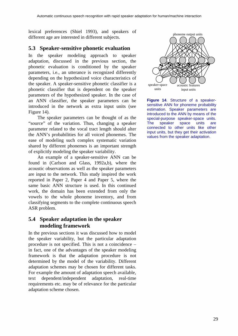
5.3 Speaker-sensitive phonetic evaluationIn the speaker modeling approach to speakeradaptation, discussed in the previous section, thephonetic evaluation is conditioned by the speakerparameters, i.e., an utterance is recognized differentlydepending on the hypothesized voice characteristics ofthe speaker. A speaker-sensitive phonetic classifier is aphonetic classifier that is dependent on the speakerparameters of the hypothesized speaker. In the case ofan ANN classifier, the speaker parameters can beintroduced in the network as extra input units (seeFigure 14).

The speaker parameters can be thought of as the“source” of the variation. Thus, changing a speakerparameter related to the vocal tract length should alterthe ANN’s probabilities for all voiced phonemes. Theease of modeling such complex systematic variationshared by different phonemes is an important strengthof explicitly modeling the speaker variability.

An example of a speaker-sensitive ANN can befound in (Carlson and Glass, 1992a,b), where theacoustic observations as well as the speaker parametersare input to the network. This study inspired the workreported in Paper 2, Paper 4 and Paper 5, where thesame basic ANN structure is used. In this continuedwork, the domain has been extended from only thevowels to the whole phoneme inventory, and fromclassifying segments to the complete continuous speechASR problem.

5.4 Speaker adaptation in the speakermodeling framework

In the previous sections it was discussed how to modelthe speaker variability, but the particular adaptationprocedure is not specified. This is not a coincidence –in fact, one of the advantages of the speaker modelingframework is that the adaptation procedure is notdetermined by the model of the variability. Differentadaptation schemes may be chosen for different tasks.For example the amount of adaptation speech available,text dependent/independent adaptation, real-timerequirements etc. may be of relevance for the particularadaptation scheme chosen.

speaker-spaceunits

acoustic featuresinput units

phoneme output units

Figure 14 . Structure of a speaker-sensitive ANN for phoneme probabilityestimation. Speaker parameters areintroduced to the ANN by means of thespecial-purpose speaker-space units.The speaker space units areconnected to other units like otherinput units, but they get their activationvalues from the speaker adaptation.

Nikko Ström

30

Clearly, speaker adaptation in the speakermodeling framework includes, in one form or the other,estimation of the current speaker’s position in thespeaker-space. If the speaker’s position is known, thisinformation can be used to condition the phoneticevaluation, and give a more accurate recognition. If theexact position in the speaker-space is unknown, it mustbe estimated from the knowledge sources at hand. Thisincludes speech recorded previously from the speaker(possibly only the one utterance to recognize), but itcould also include other types of information that isavailable to the system. For the analysis of the recordedspeech, features that are often discarded in ASR canpotentially be of use for the speaker characteristicsestimation, e.g., fundamental frequency, that is stronglycorrelated with gender.

The estimation of speaker-space position needs notbe explicit. An useful concept is the so called speakerconsistency principle. This is a formulation of theobservation that an utterance is spoken by one and thesame speaker, from the beginning to the end. Thisconstrains the observation space and can therefore beused to reduce the variation in the ASR model. In thespeaker modeling framework, the speaker consistencyprinciple can be introduced by enforcing constantspeaker parameters throughout the utterance. This canbe implemented by adding a new dimension to thesearch space of the dynamic decoding. The original twodimensions: time and HMM state, are thencomplemented with the third dimension of the speakerparameters. This is the method used in Paper 5. Theextended search space is illustrated in Figure 15.

The dynamic decoding search in the extendedsearch space of Figure 15 is pruned with beam-pruningjust like in the case of the standard search in twodimensions. The effect is that partial hypotheses withlow probability will not be further investigated in thesearch, leaving more computational resources for themore promising hypotheses. In the extended searchspace, a part of a hypothesis is the speakercharacteristics, so the effect of beam pruning is thathypotheses with unlikely speaker parameters will bepruned. In effect this is speaker adaptation – as theViterbi search progresses, unlikely speakercharacteristics are successively pruned, and thespeaker’s position in the speaker space will graduallybe more specified. Consequently, more resources can beallocated for the other dimension. Thus, in thisframework, adaptation in the sense that something in

HMM states

time

speakercharcteristics

HMM states

time

Figure 15 . Search-space of thedynamic decoding. Top: the standardsearch space with the two dimensionstime and HMM states. The objective ofthe dynamic decoding is to find themost likely path through the search-space. Because of beam-pruning,many paths in the search space arenever investigated. This is indicated bythe shadowed “beam” in the figure.Bottom: the search space with anadditional dimension of speakercharacteristics. At the beginning of thesearch, all possible speakercharacteristics are inside the beam,but as the search progresses, unlikelyspeaker characteristics aresuccessively pruned, and thespeaker’s position in the speakerspace is gradually more specified.


31

the system is progressively changed, is the changedbalance of attention in the search from speakercharacteristics to HMM states.

As a final note, we point out that the speakermodeling approach and speaker consistency modelingdo not require an ANN model – a related adaptationscheme in the HMM domain is found in a paper byLeggeter and Woodland (1994), and a slightly differentapproach to implement the speaker consistencyprinciple is taken by Hazen and Glass (1997). In theirconsistency model, the key concept is long rangecorrelation between speech sounds. No explicit speakermodel is used, but the method is successfully combinedwith speaker clustering and a technique called“reference speaker weighting”. Both of these implicitlydefine speaker models by the space spanned by theclusters and reference speakers respectively.

Nikko Ström

32

6. Applications

6.1 The WAXHOLM dialoguedemonstrator

The WAXHOLM human-machine dialoguedemonstrator is built on a generic framework forhuman/machine spoken dialogue under continuousdevelopment at the speech group at the department forSpeech, Music and Hearing of KTH. The domain of theWAXHOLM application is boat traffic and touristinformation about hotels, camping grounds, andrestaurants in the Stockholm archipelago. Theapplication database includes timetables for a fleet ofsome twenty boats from the Waxholm company, whichconnects about two hundred ports. The user input to thesystem is spoken language exclusively, but theresponses from the system include synthetic speech aswell as pictures, maps, charts and timetables (see Figure16).

The ASR module of the system, described in detailin Paper 4, has a domain-dependent vocabulary ofabout 1000 words. The application has similarities tothe ATIS domain within the ARPA community, theVoyager system from MIT (Glass et al., 1995) andEuropean systems such as SUNDIAL (Peckham, 1993),Philips’s train timetable information system (Aust etal., 1994) and the Danish dialogue project (Dalsgaardand Baekgaard, 1994). Summaries of the WAXHOLMdialogue system and the WAXHOLM project databasecan be found in (Bertenstam et al. 1995a,b) and an earlyreference is Blomberg et al. (1993).

The demonstration system is currently matureenough to be displayed and tested outside the laboratoryby completely novice users. A successful such attemptwas made at “Tekniska Mässan” (the technology fair)in Älvsjö in October ’96. Visitors with no priorexperience with the system were invited to try thedemonstrator in a rather noisy environment.

Grammar &Semantics

AutomaticSpeech

Recognition

DatabaseSearch

Data base

GraphicsSpeech synthesis(face and sound) Sound

DialogueManager

Record

Lexicon

INPUT

OUTPUT

Ship schedulesPort locationsLodgingEating

Charts Maps Tables Speech

WordsParts of speechSemantic informationPronunciation

Context sensitive rulesTransition networks

Recordings

Speech

Figure 16 . Overview of theWAXHOLM demonstrator system. Seethe main text for details.


33

6.2 An instructional system for teachingspoken dialogue systems technology

Human/machine dialogue systems are large complexsoftware projects, and have traditionally required highexpertise to design and develop. However, recentlyefforts have been made to make this type of userinterface available for developers that are not experts inthe area. Central to this development are the modulartoolkits that are being developed, e.g., OGI’s CSLUsh(Sutton et al., 1996), and MIT’s Sapphire (Hetheringtonand McCandless, 1996) toolkits. A toolkit in the samespirit is also being developed at the department forSpeech, Music and Hearing (Sjölander and Gustafson,1997). Existing components for speech recognition,speech synthesis, visual speech synthesis and NLP toolshave been extracted and re-designed to fit in a commonframework under the Tcl language. The Tcl languagehas many shortcomings, but is convenient for rapidprototyping and development work on the systemintegration level, and offers good graphical supportthrough the accompanying Tk-widget set. The ASRsystem described in the previous sections developed forthe WAXHOLM system is the underlying speechrecognition module of the toolkit.

The increased availability of the technology makesstudent courses in the subject matter possible. A simple,but fully functioning dialogue instructional system hasbeen developed using the toolkit for educationalpurposes (Sjölander and Gustafson, 1997). The systemhas been used for courses at the MSc level at KTH, andat Linköping University in Sweden. In thisenvironment, students are presented with a simplespoken dialogue application for yellow pages search ona few selected topics using voice input. The applicationis accompanied by a development environment thatallows the students to interactively follow theprocessing in the system and modify the differentmodules even while it runs. A screen-shot of the systemin use is shown in Figure 17

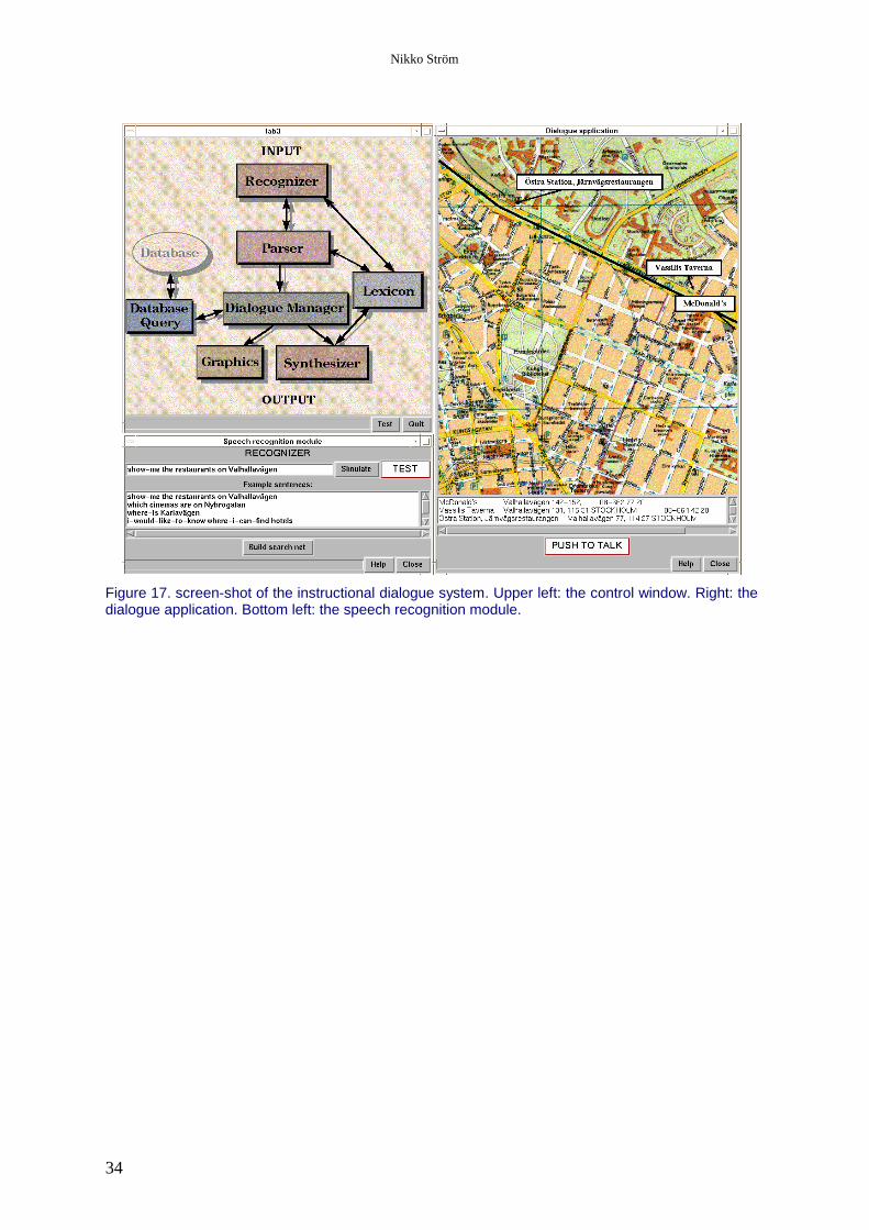
Nikko Ström

34

Figure 17. screen-shot of the instructional dialogue system. Upper left: the control window. Right: thedialogue application. Bottom left: the speech recognition module.


35

7. Summaries and comments on individualpapers

7.1 Paper 1.This paper was written after the first implementation ofthe ASR module of the WAXHOLM demonstrationsystem. Since then, the system has continuously beenimproved, and has been one of the main tools for theexperiments of this thesis.

The A* algorithm is defined in a graph formalism,where both the input and output of the algorithm, andthe lexicon and grammar model are represented bydirected graphs. The acoustic input observation of anutterance, and the word sequence hypotheses that arethe output, are represented by graphs called observationgraphs. The nodes of observation graphs have a time-tag, and arcs between the nodes represent some aspectof the observation between the two times. The graphrepresenting the lexicon and grammar model is aprobabilistic finite state automaton, e.g., an HMM. Thegraph formulation of the A* algorithm is also used inPaper 3 and has been a useful conceptual tool in thedevelopment of the search.

A large part of the paper is concerned withcomputational aspects of the search. CPU and memoryrequirements are discussed for the implementation ofthe first pass of the A* algorithm, but it is the graphreduction methods in the second, stack-decoding, passof the implantation that is the most importantcontribution of this paper. The idea is to utilize theregularities of the words in the lexicon to reduce theeffective search space. For example, many words beginwith the same phoneme, and it is not necessary toevaluate them more than once at a particular time. Thisnotion is generalized with the help of quotient graphs.The quotient graph is typically a significantly smallergraph than the original model graph, but all nodes ofthe original graph have a corresponding node in thequotient graph. The search can be made in the quotientgraph, and when a search result is needed for a node inthe original graph, there is always a reference to aquotient graph node where the result is available.

"Optimising the LexicalRepresentation to Speed Up A*Lexical Search,"STL QPSR 2-3/1994, pp. 113-124.

Nikko Ström

36

7.2 Paper 2In this report the speaker sensitive ANN, introduced inStröm (1994b), is further investigated. The generalframework, an ANN for phoneme evaluation with a setof extra input units that characterizes the speaker isinspired by the work of Carlson and Glass (1992a,b),and is also used in Paper 5 and discussed in Paper 4.

In this report, the speaker parameters supplied bythe extra input units are automatically extracted, i.e.,they have no explicit relation to any knowledge-basedparameters. However, using a novel analysis-by-synthesis method, the influence of the automaticallyextracted parameters was visualized in the formantspace. An ensemble of synthetic vowels were generatedby a formant synthesizer driven by an LF voice source(Fant, Liljencrants and Lin, 1985). The individualvowels of the ensemble were varied only in F1 and F2,(the first and second formant frequencies). Thesynthetic vowels were then fed to the ANN and thevowel classification was recorded. This makes itpossible to draw a map with the phoneme boundaries inthe F1/F2 space for the ANN. By repeating theprocedure with different speaker parameters, the effectof the speaker parameters on the phoneme boundariescan be studied. It was found that, in agreement withtheory, the phoneme boundaries were lower infrequency for speaker parameters corresponding to malevoices than female. In another analysis, a correlationbetween the knowledge-based parameter fundamentalfrequency, and one of the two automatically generatedparameters was also found.

This report was written during my stay as a guestresearcher at ATR, Kyoto, Japan. As a curiosity I canmention that, as part of my attempt to learn theJapanese language, it was written on a Macintosh withonly Japanese labels on all buttons and menu items.However, I never quite succeeded in learning the kanjicharacters, so sometimes some pretty spectacular thingshappened on the screen. This was how I learned torecognize the “undo” character.

"A Speaker Sensitive ArtificialNeural Network Architecture forSpeaker Adaptation,"ATR Technical Report, TR-IT-0116, 1995,ATR, Japan.


37

7.3 Paper 3This paper presents the status of the continuous speechrecognition engine of the WAXHOLM project at theend of 1996. At this point the demonstration systemwas mature enough to be displayed and tested outsidethe laboratory by completely novice users. A successfulsuch attempt was made at “Tekniska Mässan” (thetechnology fair) in Älvsjö in October ’96 where visitorswith no prior experience with the system were invitedto try the demonstrator in a rather noisy environment.

All parts of the ASR module are described in somedetail in the paper, including the different modes ofoperation: standard CDHMM, hybrid HMM/ANN, anda general phone-graph input mode. However, the focusis on the aspects of the system that are original in somesense, and the ANN part of the system is covered morethoroughly in Paper 6.

Most of the report is devoted to the dynamicdecoding block of the system. The graph representationof the search space of the dynamic decoding isdescribed in detail, and algorithms for graph reduction,Viterbi search, and A* stack decoding are given.

The optimization of the lexical graph is perhapsthe most original aspect of the decoding block of thesystem. This is a continuation of the work reported inPaper 1. The resulting graph has only one word-end andone word-start node for each word class. This results ina very small number of word connecting arcs. Withoutthe graph reduction, the algorithm would spend a largepart of its CPU time processing the word connectingarcs. The key concept that was utilized to achieve thishigh degree of reduction is word pivot arcs. This is aninnovation that was not used in Paper 1.

For the estimation of bigram grammarprobabilities, a novel estimate based of Zipf’s law forword frequency is proposed. However, theWAXHOLM corpus is not large enough for aconclusive judgment of the method.

"Continuous Speech Recognitionin the WAXHOLM DialogueSystem,"STL QPSR 4/1996, pp. 67-96.

Nikko Ström

38

7.4 Paper 4This book illuminates the subject of talker variabilityfrom the different viewpoints of research in auditoryword recognition, speech perception, voice perceptionand ASR. A common theme of all chapters is toapproach speaker variability as a source of informationrather than unwanted noise. In particular in the ASRfield, the latter have often been the case in the past. Theapproach is very apparent in my chapter, that describesthe ideas behind the experiments with fast speakeradaptation, reported on in Paper 2 and Paper 5. Theconcepts of a speaker space, and an explicit model forthe speaker variability are laid out.

The chapter also contains a survey of existingspeaker adaptation methods, and comparison withadaptation effects in the human speech perceptionprocess is made.

"Speaker Modeling for SpeakerAdaptation in Automatic SpeechRecognition,"in: Talker Variability in SpeechProcessing, Chapter 9, pp. 167-190, Eds: Keith Johnson and JohnMullennix, 1997, Academic Press.


39

7.5 Paper 5This is the latest included paper on fast speakeradaptation. In this paper, the speaker modelingapproach introduced in (Ström, 1994b), and developedfurther in Paper 2, is used in a full continuous speechrecognition experiment.

The adaptation performance was evaluated on theWAXHOLM database. Overall, the adaptation effectwas not very high, but the database contains a largeportion of very short utterances (only a few words), andthis was not enough for the adaptation to give a positiveeffect. On average the adaptation had positive effect onthe word-error rate for utterances longer than threewords, but increased the word-error rate for shorterutterances. The utterance level result, i.e., the fractioncompletely correctly recognized utterances, was incontrast, slightly improved for all utterance lengths.

Although it was shown that the proposedadaptation method can improve recognition both at theword and utterance level, the merit of this paper is notthe results achieved. The ANN used in the study israther small, the speaker space used in the experimentsis simplistic (only two speaker parameters), and thesampling of the speaker space is coarse. The maincontribution of this paper is that it showed that themethod is feasible in a full ASR system.

"Speaker Adaptation by Modelingthe Speaker Variation in aContinuous Speech RecognitionSystem,"Proc. ICSLP '96, Philadelphia, pp.989-992.

Nikko Ström

40

7.6 Paper 6This paper focuses on the latest development of, andprovides detailed information on a complete ANNtoolkit, developed during the course of my thesisstudies. The department of Speech, Music and Hearingat KTH has a history of research in the area (Eleniusand Takacs, 1990), and the first step of the developmentof the toolkit is reported on in Ström, 1992. Formulaeare given for back-propagation training of thegeneralized dynamic ANN architecture used. Thedynamic networks require that units’ activities arecomputed in a particular, time-asynchronous order, andan algorithm for computing this order is described indetail. All aspects of network training and evaluationare discussed; network topology, weight initialization,input feature representation, the “softmax” outputactivation function, and the theory that establishes thelink between multi-layer perceptrons and a posterioriphoneme probabilities.

This paper also announces the toolkit as a publiclyavailable software resource, available for free by theresearch community. In an appendix, detailedinstructions are given for training and evaluating ANNsfor phoneme probability estimation using the toolkit.The source code and documentation are available on theInternet. To this date, the toolkit has been downloadedfrom more than 75 different sites worldwide.

The innovative part of the paper is the sparseconnection and connection pruning of the networks,that to my knowledge have not been used for phoneprobability estimation ANNs before. The sparseconnectivity of the networks allows considerablyenlarged hidden layers without increasing thecomputational demands, and this is shown to improverecognition accuracy significantly. The phonemerecognition results for the TIMIT database are in therange of the lowest error-rate reported, and outperformsall HMM based systems for the core test set of thedatabase.

Since this paper was published, the development ofthe toolkit, and a new ANN architecture have resultedin further improvement of the phoneme recognition.Currently our lowest error-rate for the core test set ofthe TIMIT database is 26.7% (Ström, 1997). Thedevelopment of other systems have also resulted inreduced error-rates, Chang and Glass (1997) report anerror-rate of 26.6% using their segment based approach.

"Phoneme Probability Estimationwith Dynamic Sparsely ConnectedArtificial Neural Networks," TheFree Speech Journal, Vol. 1(5),1997.


41

AcknowledgmentsFirst of all, I would like to thank Evolution for comingup with the brilliant idea of using the same device forchewing, breathing, and emitting sounds forcommunication, making automatic speech recognitionone of the most challenging engineering tasks one canthink of.

I am grateful to my colleagues for making my workenvironment so stimulating, both at KTH, and duringmy stay as a guest researcher at ATR. In particular RolfCarlson has given important guidance over the wholeperiod. It was also studies of Rolf Carlson and JamesGlass that inspired to my work in the area of speakeradaptation. Michael Phillips deserves acknowledgmentfor introducing me to the A* algorithm and lexicalsearch algorithms, and Kjell Elenius has always been agood conversation partner in ANN related issues.

Further, I would like to thank Björn Granström forallowing me to work in this area, and for guidance andinspiration. I would also like to thank YoshinoriSagisaka for inviting me to work in the stimulatingresearch environment at ATR in Kyoto, Japan.

I also take the opportunity to thank all my teachers,all the way from kindergarten to graduate courseteachers. Of course, this thesis would have beenimpossible without them.

I thank my mother and father for all their support,and for providing a home where education was anatural part of life. All my friends deserveacknowledgment for being so patient with me when Ioccasionally completely forget about everything but mywork. Finally, thank you Linda for love, support, andunderstanding.

My first two years of doctoral studies were sponsoredby a donation by VOLVO AB, and the remainingstudies were financially supported by NUTEK andHSFR, and during the last year also by CTT, a centerfor speech technology, jointly sponsored by, NUTEK,Swedish industry and KTH.

Nikko Ström

42

ReferencesAhadi S. M. and Woodland P. C. (1995) : “Rapid speakeradaptation using model prediction,” Proc. ICASSP 1995, pp.684-687.

Aust H., Oerder M., Seide F., and Steinbiss V. (1994) :“Experience with the Philips automatic train timetableinformation system,” Proc. of IEEE Workshop onInteractive Voice Technology for TelecommunicationsApplications (IVTTA94), pp. 67-72.

Bertenstam J., Blomberg M., Carlson R., Elenius K.,Granström B., Gustafson J., Hunnicutt S., Högberg J.,Lindell R., Neovius L., de Serpa-Leitao A., and Ström N.(1995a) : “The Waxholm application database,” Proc.EUROSPEECH '95, Madrid, pp. 833-836.

Bertenstam J., Blomberg M., Carlson R., Elenius K.,Granström B,. Gustafson J., Hunnicutt S., Högberg J.,Lindell R., Neovius L., de Serpa-Leitao A., Nord L., andStröm N. (1995b) : “Spoken dialogue data collection in theWaxholm project,” STL-QPSR, KTH, 1/1995, pp. 50-73.

Blomberg M., Carlson R., Elenius K., Granström B.,Gustafson K., Hunnicutt S., Lindell R., and Neovius L.(1993) : “An experimental dialogue system: Waxholm,”EUROSPEECH '93, pp. 1867-1870.

Bourlard H. (1995) : “Towards increasing speechrecognition error rates,” Proc. EUROSPEECH ’95, pp. 883-894.

Bourlard H. and Morgan N. (1993) : “Continuous speechrecognition by connectionist statistical methods,” IEEEtrans. on Neural Networks, Vol. 4(6), pp. 893-909.

Bourlard H. and Wellekens C. J. (1988) : “Links betweenMarkov Models and Multilayer Perceptrons,” IEEE Transon PAMI, 12(12), pp. 1167-1178.

Brown P. F., Lee C-H, and Spohrer J. C. (1983) : “Bayesianadaptation in speech recognition,” Proc. ICASSP 1983, pp.761-764.

Carlson, R. and Glass J. (1992a) : “Vowel classificationbased on analysis-by-synthesis,” STL-QPSR 4/1992, pp. 17-27, Dept. of Speech Communication and Music Acoustics,KTH, Sweden.

Carlson R. and Glass J. (1992b) : “Vowel classificationbased on analysis-by-synthesis,” Proc. ICSLP 1992, pp.575-578.

Carlson R. and Hunnicutt S. (1996) : “Generic and domain-specific aspects of the Waxholm NLP and dialog modules”Proc. ICSLP 1996, pp. 677-680.


43

Chang J. and Glass J. (1997) : “Segmentation and modelingin segment-based recognition,” Proc. EUROSPEECH 1997,pp. 1199-1202.

Cohen J. (1996): “The summers of our discontent,” Proc.ICSLP 1996, distributed on CDROM version.

Dalsgaard P. and Baekgaard A. (1994) : “Spoken languagedialogue systems,” Proc. of Artificial Intelligence, Infix.Presented at the CRIM/FORWISS workshop on Progressand Prospects of Speech Research and Technology, Munich.

Digalakis V. V., Ostendorf M., and Rohlicek J. R. (1992) :“Fast algorithms for phone classification and recognitionusing segment-based models,” IEEE Trans. on SignalProcessing, Vol. 40, pp. 2885-2896.

Elenius K. and Takacs G. (1990) : “Acoustic-phoneticrecognition of continuos speech by artificial neuralnetworks,” STL-QPSR 2-3/1990, pp. 1-44, KTH, Dept. ofSpeech Communication and Music Acoustics, Sweden.

English T. M. and Boggess L. C. (1992) : “Back-propagation training of a neural network for word spotting”,Proc. ICASSP ´92, Vol. 2, pp. 357-360.

Fant G., Liljenkrans J., and Lin Q. (1985) : “A four-parameter model of glottal flow,” STL-QPSR 4/85, pp. 1-13,KTH, Dept. of Speech, Music and Hearing, Sweden.

Gauvain J. L. and Lee C. H. (1994) : “Maximum a posterioriestimation for multivariate Gaussian observations ofMarkov chains,” IEEE Trans. Speech and Audio Processing,Vol. 2(2), pp. 806-814.

Gish H. (1990) : A probabilistic approach to theunderstanding and training of neural network classifiers,”Proc. ICASSP '90, pp.1361-1364.

Glass J., Chang J., and McCandless M. (1996) : “Aprobabilistic framework for feature-based speechrecognition,” Proc. ICSLP ’96, pp. 2277-2280.

Glass J., Flammia G., Goodine D., Phillips M., Polifroni J.,Sakai S., Seneff S., and Zue V. (1995) : “Multilingualspoken language understanding in the MIT voyager system,”Speech Communication 17/1-2, pp. 1-18.

Hazen T. J. and Glass J. R. (1997) : “A comparison of noveltechniques for instantaneous speaker adaptation,” Proc.EUROSPEECH 1997, pp. 2047-2050.

Hetherington L. and McCandless M. (1996) : “SAPPHIRE:An extensible speech analysis and recognition tool based onTcl/Tk,” Proc ICSLP ’96, pp. 1942-1945.

Hetherington L., Phillips M., Glass J., and Zue V. (1993) :“A* word network search for continuous speechrecognition,” ICASSP '93, pp. 1533-1536.

Nikko Ström

44

Hopcroft J. and Ullman J. (1979) : Introduction to automatatheory, languages and computation, Addison and Wesley,ISBN 0-201-02988X.

Huang X. D. and Lee K. F. (1991) : “On speaker-independent, speaker-dependent and speaker-adaptivespeech recognition,” Proc. ICASSP 1991, pp. 877-880.

Kershaw D. J., Hochberg M. M., and Robinson A. J. (1996): “Context-dependent classes in a hybrid recurrent network-HMM speech recognition system,” In Advances in NeuralInformation Processing Systems, Vol. 8, eds: Touretsky D.S., Mozer M. C, and Hasselmo M. E., Morgan Kaufmann.

Ladefoged P., and Broadbent D. E. (1957) : “Informationconveyed by vowels,” JASA 29(1), pp. 99-104.

Le Cun Y., Denker J. S., and Solla S. A. (1990) : “Optimalbrain damage,” In Advances in Neural InformationProcessing Systems Vol. II , ed: Touretsky D. S., pp. 589-605, San Mateo, California IEEE, Morgan Kaufmann.

Leggetter C. J. and Woodland P. C. (1994) : “Speakeradaptation of continuous density HMMs using multivariatelinear regression,” Proc. ICSLP 1994, pp. 451-454.

Levin E. (1990): “Word recognition using hidden controlneural architecture”, Proc. ICASSP '90, Vol. 1, pp. 433-436.

Li K. P., Naylor J. A., and Rossen M. L. (1992) : “A wholeword recurrent neural network for keyword spotting,” Proc.ICASSP ´92, Vol. 2, pp. 81-84.

Mitchel C. D., Harper M. P., and Jamieson L. H. (1996) :“Stochastic observation hidden Markov models,” Proc.ICASSP '96, pp. 617-620.

Necioglu B. F., Ostendorf M., and Rohlicek J. R. (1992) :“A Bayesian approach to speaker adaptation for thestochastic segment model,” Proc. ICASSP 1992, pp. I-437 -I-440.

Ney H. and Aubert X. (1994) : “A word graph algorithm forlarge vocabulary, continuous speech recognition,” Proc.ICSLP '94, pp. 1355-1358.

Peckham J. (1993) : “A new generation of spoken dialogsystems: results and lessons from the SUNDIAL Project,”Proc. Eurospeech ’93; pp. 33-40.

Richard M. D. and Lippman R. P. (1991) : “Neural networkclassifiers estimate Bayesian a posteriori probabilities,”Neural Computation, Vol. 3, pp. 461-483.

Robinson A. J. (1994) : “An application of recurrent nets tophone probability estimation,” IEEE trans. on NeuralNetworks Vol. 5(2), pp. 298-305.

Robinson T. and Fallside F. (1991) : “A recurrent errorpropagation network speech recognition system,” ComputerSpeech & Language 5:3, pp. 259-274.


45

Shiel F. (1993) : “A new approach to speaker adaptation bymodelling pronounciation in automatic speech recognition,”Speech Communication Vol. 13, pp. 281-286.

Sietsma J. and Dow R. J. F. (1991) : “Creating artificialneural networks that generalize,” Neural Networks, 4(1) pp.67-69.

Sjölander K. and Gustafson J. (1997) : “An integratedsystem for teaching spoken dialogue systems technology,”Proc. EUROSPEECH ‘97, pp. 1927 - 1930.

Soong and Huang (1991) : “A tree-trellis based fast searchfor finding the N best sentence hypotheses in continuousspeech recognition,” Proc. ICASSP ‘91, pp. 713-716.

Strange W. (1989): “Evolving theories of vowelperception,” JASA 85(5), pp. 2081-2087.

Ström N. (1992): “Development of a recurrent time-delayneural net speech recognition system,” STL-QPSR 2-3/1992,pp. 1-44, KTH, Dept. of Speech Communication and MusicAcoustics, Sweden.

Ström N. (1994a) : “Optimising the lexical representation toimprove A* lexical search”, STL-QPSR 2-3/1994, pp. 113-124.

Ström N. (1994b): “Experiments with a new algorithm forfast speaker adaptation,” Proc. ICSLP 1994, pp. 459-462.

Ström N. (1995): Generation and minimisation of wordgraphs in continuous speech recognition,” Proc. Workshopon Automatic Speech Recognition, pp. 125-126, Snowbird,Utah.

Ström N. (1997): Nikko Ström (1997): “A tonotopicartificial neural network architechture for phonemeprobability estimatio,” To appear in Proc. of the 1997 IEEEWorkshop on Speech Recognition and Understanding, SantaBarbara, CA.

Sutton S., de Veilliers J., Schalkwyk J., Fanty M., Novick D.and Cole R. (1996): “Technical specification of the CSLUtoolkit;” Tech. Report No. CSLU-013096, CSLU, Dept. ofComputer Science and Engineering, Oregon GraduateInstitute of Science and Technology, Portland. OR.

Tebelskis J. and Waibel A. (1990): “Large vocabularyrecognition using linked predictive neural networks,” Proc.ICASSP '90, Vol. 1, pp. 437-440.

Verbrugge R. R. and Strange W. (1976): “What informationenables a listener to map a talker’s vowel space,” JASA60(1), pp. 198-212.

Viterbi A.J. (1967): “Error bounds for convolutional codesand an asymptotically optimum decoding algorithm,” IEEETrans. Information Theory, Vol. IT-13, pp. 260-269.

Nikko Ström

46

Waibel A., Hanazawa T., Hinton G., Shikano K. and LangK. (1987) : “Phoneme recognition using time-delay neuralnetworks,” ATR Technical Report TR-006, ATR, Japan.

automatic continuous speech recognition with rapid speaker adaptation for human/machine

Documents