automatic control and system theory - … · control of digital systems g. palli (dei) automatic...

Control of Digital Systems

Automatic Control & System Theory 1 G. Palli (DEI)

AUTOMATIC CONTROL AND SYSTEM THEORY

CONTROL OF DIGITAL SYSTEMS

Gianluca Palli

Dipartimento di Ingegneria dell’Energia Elettrica e dell’Informazione (DEI) Università di Bologna

Email: [email protected]

TexPoint fonts used in EMF. Read the TexPoint manual before you delete this box.:


G. Palli (DEI) Automatic Control & System Theory 2

Analog Control Systems

Analog Control Systems ü  The computation of the control action is carried out in the

continuous-time domain, by means of electric, hydraulic or mechanical systems

Controller plant

transducer

power amplifier actuator

+

-



Digital Control Systems

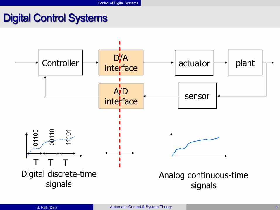
Digital Control Systems ü  A computer is present in the control loop:

ü The control action is computed in the discrete-time domain with period T

ü  Suitable interfaces are needed between: ü The plant (continuous time domain) ü The controller (discrete time domain)

plant

transducer

actuator DIGITAL COMPUTER D/A A/D

Clock (T)

Discrete-time domain

10

10

11

00

+

-



Digital Control Systems vs. Analog Control Systems

• Better precision and computational capabilities •  More complex control algorithms

•  Improved flexibility •  Different operating conditions can be managed

by just changing the software

• Better reliability and repeatability •  No fatigue, thermal drift etc.

• Digital signals can be easily transmitted •  Digital signals are more robust than analog ones

with respect to noise and disturbances

• A more difficult design process •  The designer must possess competences in

the field of electronics and digital interfaces

• Weaker stability •  Transmission discontinuities, delays •  The choice of the sampling time is important

• Undesired and unmanaged system failures •  It is difficult to consider and evaluate all the

possible failures during the software design

• Electric power is always needed



Signals Typologies

Analog continuous-time Sampled

data

Digital signal (quantized) Quantized continuous-time



Digital Control Systems

Analog continuous-time signals

Digital discrete-time signals

T

0110

0

T

0011

0

T

1110

1 D/A

interface plant Controller

sensor

actuator

A/D interface



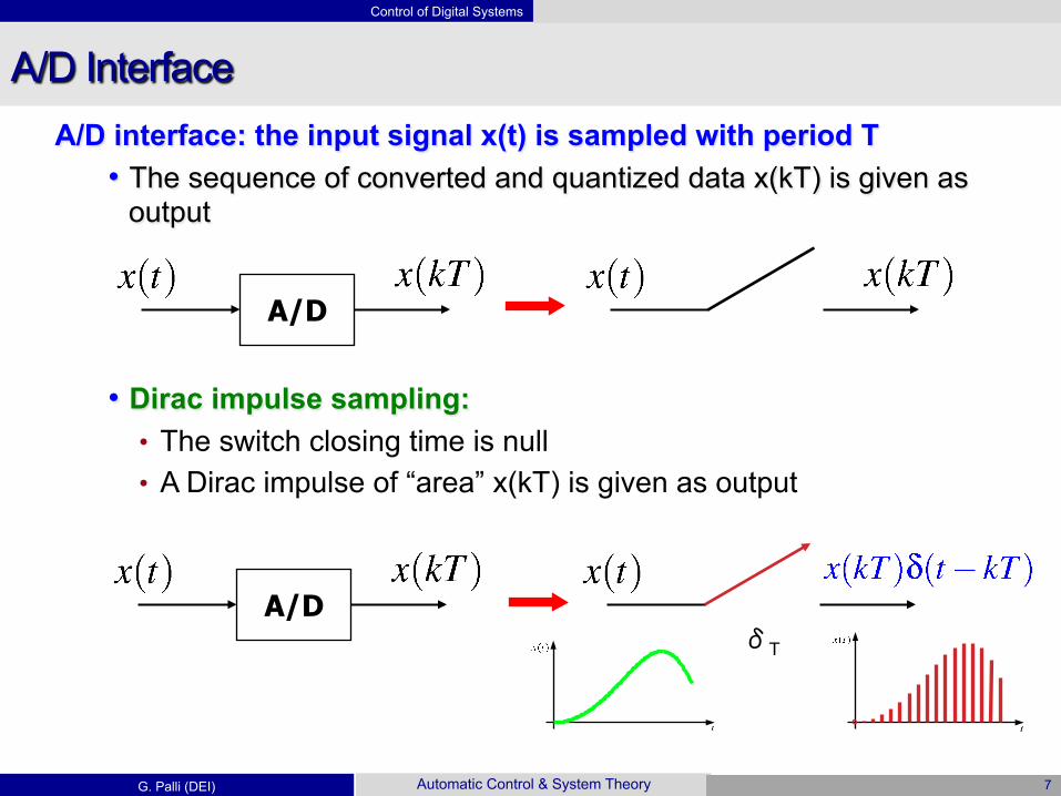
A/D Interface A/D interface: the input signal x(t) is sampled with period T

• The sequence of converted and quantized data x(kT) is given as output

• Dirac impulse sampling: •  The switch closing time is null •  A Dirac impulse of “area” x(kT) is given as output

A/D

A/D δT



• Provides an analog signal from the input sequence of sampled data •  The solution of the signal reconstruction problem is not unique if the

SHANNON THEOREM is not satisfied (ωs > 2 ωc, ωs = 2 π/T)

• Zero-Order Hold gives the output:

•  Assuming an ideal sampling:

D/A Interface



Two approaches are possible to the design of digital control laws: 1.  “Direct” method

•  Discretization of the plant model •  Design of the controller in the discrete-time domain

2.  “Indirect” Method •  Simplest approach, it does not requires specific knowledge of

design techniques in the discrete-time domain •  Some limitations are given by the choice of the sampling time

Design of Discrete-Time Controllers



Digit

• Indirect method (discretization)

R(s) G(s) x(t) e(t) ua(t) ya(t)

R(z) G(s) x(t) e(t) ua(t) ya(t)

H(s)

•  T = … ? (as small as possible…)




With the “indirect” method, four steps are usually involved: 1.  Choice of the sample time T

2.  Design of the continuous–time control law R(s)

3.  Discretization of the control function R(s) (e.g. bilinear transformation)

4.  Verification of the result by simulation (and experiments)




Digit Design of digital controllers

1) Choice of T and verification of the stability margins of the system

•  In designing the control law R(s), the process to be considered is




•  Example: Given the system

Design a digital lag net such that the phase margin results Mf = 55o

The smallest time constant, corresponding to the pole in p = -2, is τ = 0.5 s. Then, consider the sample time T = 0.1 s.

Impulse Response

Time (sec)

Am

plitu

de

0 1 2 3 4 5 6 7 8 9 100

0.1

0.2

0.3

0.4

0.5

0.6

0.7

0.8

0.9

1




Bode diagrams of the original transfer function and of the sampled one Bode Diagram

Frequency (rad/sec)

Phas

e (d

eg)

Mag

nitu

de (d

B)

-100

-80

-60

-40

-20

0

20

10-1 100 101-360

-315

-270

-225

-180

-135

-90

G(s)

G(z)



Digit

Nyquist Diagram

Real Axis

Imag

inar

y A

xis

-2 -1.5 -1 -0.5 0 0.5 1-2

-1.5

-1

-0.5

0

0.5

1

1.5

2

Design of digital controllers

• Considering the zero-order hold, the following system is obtained

G(s)

G1(s)

There is a small increase of the phase lag.

In this case, is “small” since T is small.

A similar result is obtained

with the approximation




•  Let then consider G1(s) instead of G(s)

•  The result of the design of the lag net for G1(s) (phase margin MF = 55o) is:

•  By discretization of R(s) (ex. bilinear trans.) with T = 0.1 s:

•  N.B. Possible numerical problems for “similar” numbers (round)




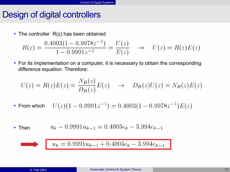
•  The controller R(z) has been obtained

•  For its implementation on a computer, it is necessary to obtain the corresponding difference equation. Therefore:

•  From which

•  Then




0 10 20 30 40 500

0.5

1

1.5

tempo (s)

Uscita del sistema

0 10 20 30 40 50-0.2

0

0.2

0.4

0.6

tempo (s)

Azione di controllo

0 1 2 3 4 50

0.2

0.4

0.6

0.81

tempo (s)

Uscita del sistema

0 1 2 3 4 50

0.1

0.2

0.3

0.4

tempo (s)

Azione di controllo

Results with T = 0.1 s




Results with T = 0.5 s

0 10 20 30 40 500

0.5

1

1.5

tempo (s)

Uscita del sistema

0 10 20 30 40 50-0.2

0

0.2

0.4

0.6

tempo (s)

Azione di controllo

0 1 2 3 4 50

0.2

0.4

0.6

0.81

tempo (s)

Uscita del sistema

0 1 2 3 4 50

0.1

0.2

0.3

0.4

tempo (s)

Azione di controllo



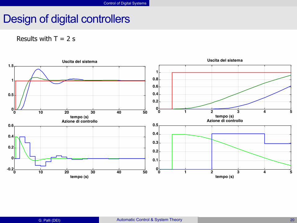
Digit Design of digital controllers Results with T = 2 s

0 10 20 30 40 500

0.5

1

1.5

tempo (s)

Uscita del sistema

0 10 20 30 40 50-0.2

0

0.2

0.4

0.6

tempo (s)

Azione di controllo

0 1 2 3 4 50

0.2

0.4

0.6

0.81

tempo (s)

Uscita del sistema

0 1 2 3 4 50

0.1

0.2

0.3

0.4

0.5

tempo (s)

Azione di controllo



Description of sampled data systems

Differential equations

Laplace transform

CONTINUOUS-TIME SYSTEMS

Finite-difference equations

Z transform

DISCRETE-TIME SYSTEMS

D/A

A/D



D/A

S&H

Plant Control algorithm

Y

Sensor

Actuator

A/D

The control algorithm must be designed in such a way that the overall control system with the same input behaves as much as possible to the continuous-time regulator R(s)

Main problem: selection of the sample time T so that the sampled– data represent a “good” approximation of the continuous-time signals

Discretization of Continuous-Time Controllers

Hold



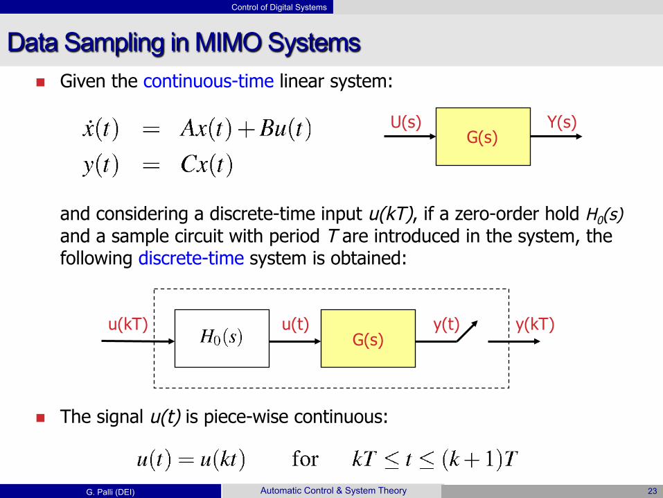
Data Sampling in MIMO Systems n  Given the continuous-time linear system:

and considering a discrete-time input u(kT), if a zero-order hold H0(s) and a sample circuit with period T are introduced in the system, the following discrete-time system is obtained:

n  The signal u(t) is piece-wise continuous:

u(kT) u(t) y(t) y(kT) G(s)

U(s) Y(s) G(s)



n  The signal u(t) is piecewise continuous:

n  The signal y(t) sampled with a period T generates the sampled signal y(kT)

u(kT) u(t)

0 2 4 6 8 10 -3

-2

-1

0

1

2

3

Tempo (sec)

Segnale y(t)

0 2 4 6 8 10 -3

-2

-1

0

1

2

3

Tempo kT (sec)

Segnale y(kT) y(kT) y(t)

for

Data Sampling



n  The input-output behavior of the overall system is the same of the discrete-time system:

G(z) U(z) Y(z)

u(kT) u(t) y(t) y(kT) G(s)

Data Sampling in MIMO Systems



n  A relation exists between matrices (A, B, C) and matrices (F, G, H). It can be computed by solving the following linear differential equation in the interval [kT, (k+1)T]:

n  The state x(t) that is reached starting from the initial state x(kT) at the time

instant t=kT is:

n  Hence, being u(t)=u(kT) constant, the state x((k+1)T) reached at the time instant t=(k+1)T is:




n  By means of the following change of variable:

the matrix G can be transformed as:

n  The output y(kT) is obtained from the signal y(t) sampled at t=kT:




n  Then, the relation between the matrices (A, B, C) and (F, G, H) is:

n  The discrete-time system G(z) obtained from the continuous-time one G(s) in this way is called sampled-data system.

n  Since matrices F and G depend on the sample time T, it is important to analyze how the structural properties of reachability and observability of the sampled-data system change in function of T.




n  Being matrix F = e AT always invertible, in the sampled data system: n  The controllability is always equivalent to reachability n  The reconstructability is always equivalent to observability

For single-input systems, the following property holds: n  THEOREM: Consider the completely reachable system (A, b) and the

sampling period T. The corresponding sampled-data system is reachable iff each couple λi , λj of distinct eigenvalues of A with the same real part satisfies the relation:

Reachability and Observability



For single-output systems, the following property holds (dual property with respect to the previous one):

n  THEOREM: Consider the completely observable system (A, c) and the sampling period T. The corresponding sampled data system is observable iff each couple λi , λj of distinct eigenvalues of A with the same real part satisfies the relation:

n  Note: If all the eigenvalues of matrix A are real, the sampled-data system maintains always, for any T > 0, the same structural characteristics (reachability, controllability, observability, reconstructability) of the original continuous-time system (A, b, c).

Reachability and Observability



n  Example: compute the matrices of the sampled-data system obtained from the following continuous-time system:

The matrices (F, G, H) result:




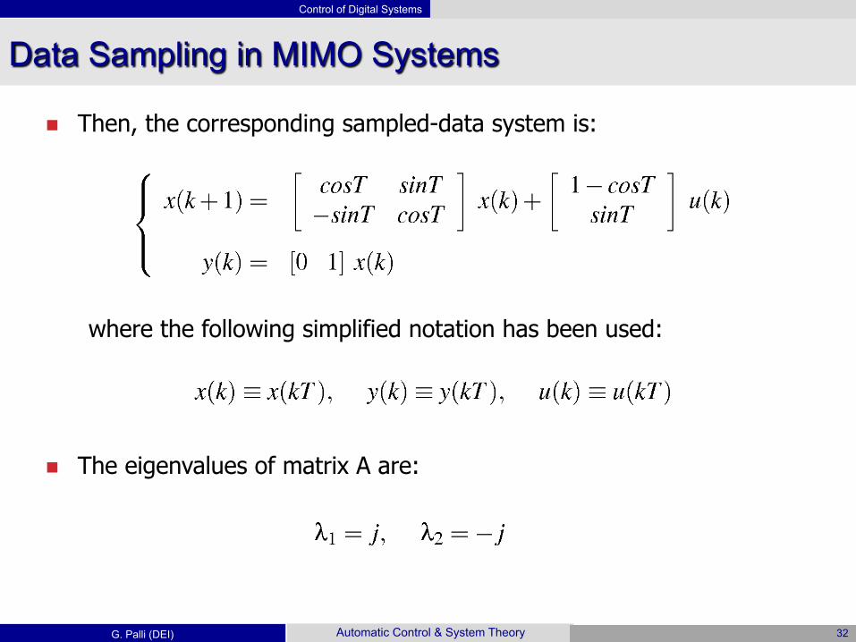
n  Then, the corresponding sampled-data system is:

where the following simplified notation has been used:

n  The eigenvalues of matrix A are:




n  The reachability matrix of the sampled-data system is:

n  For T=π the system is not fully reachable, indeed:

n  From the theorem on the reachability of sampled data systems:

Data Sampling in MIMO Systems - Reachability



n  The observability matrix of the sampled data system is:

n  The sampled data system is fully observable iff:

n  The characteristic polynomial of the matrix F is:

n  Then, the eigenvalues of F are:

Data Sampling in MIMO Systems - Observability



0 5 10 15 20 -4 -3 -2 -1 0 1 2 3 4

T = π/20

0 5 10 15 20 -15

-10

-5

0

5

10

15

T = π/2

0 5 10 15 20 -8 -6 -4 -2 0 2 4 6 8

T = π/5

0 5 10 15 20 -20 -15 -10 -5 0 5

10 15 20

T = π

Data Sampling in MIMO Systems – Impulse Response



T = π/5

T = π 0 5 10 15 20 -0.8

-0.6

-0.4

-0.2

0

0.2

0.4

0.6 0 5 10 15 20 -0.8

-0.6

-0.4

-0.2

0

0.2

0.4

0.6

0 5 10 15 20 -0.8

-0.6

-0.4

-0.2

0

0.2

0.4

0.6

T = π/20

The properties of controllability and observability degrades as the sampling period T grows

Data Sampling in MIMO Systems – Impulse Response



n  The transfer function G(s) of the continuous-time system is:

n  The transfer function G(z) of the corresponding sampled data system is:

Data Sampling in MIMO Systems – Transfer Function



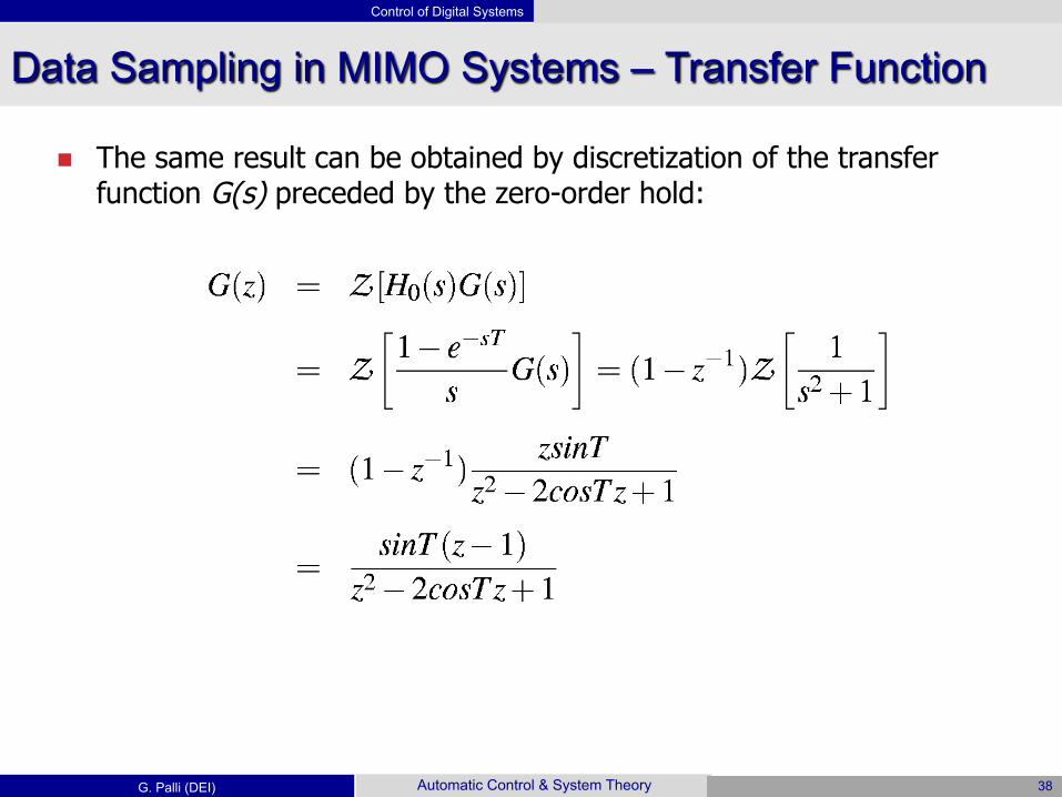
n  The same result can be obtained by discretization of the transfer function G(s) preceded by the zero-order hold:

Data Sampling in MIMO Systems – Transfer Function



n  Example: consider the following purely inertial system with unitary mass (m=1) subject to the external force u(t):

n  The state vector is given by the position and the velocity

n  The system output is the position of the mass

x

u(t) m




n  The dynamic model in the state-space representation is:

n  The matrices F and G of the corresponding sampled-data system are:




n  Therefore, the sampled-data system can be written as:

n  It can be easily verified that this system is fully reachable and observable

n  We are interested in designing a dead-beat controller: a state feedback controller u(k)=K x(k) such that all the eigenvalues of the closed-loop system eig(F+GK) are zero. This implies that the desired characteristic polynomial of the closed loop system is:




n  Assuming as state feedback matrix. Given u(k)=K x(k), the following system dynamic matrix is obtained:

n  The characteristic polynomial of this matrix is:

n  By imposing the desired characteristic polynomial we obtain:




n  Since we are considering a dead-beat controller, the state feedback u(k)=K x(t) is able to drive the state exactly to zero in just two steps (since the order of the system is two) with an arbitrary small sample time T




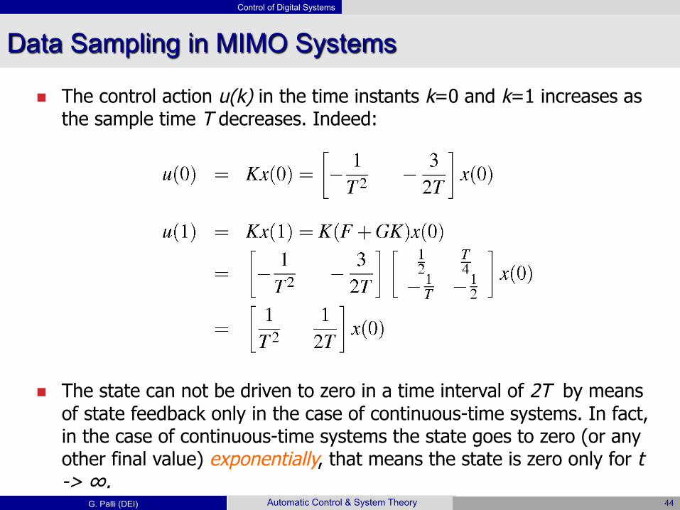
n  The control action u(k) in the time instants k=0 and k=1 increases as the sample time T decreases. Indeed:

n  The state can not be driven to zero in a time interval of 2T by means of state feedback only in the case of continuous-time systems. In fact, in the case of continuous-time systems the state goes to zero (or any other final value) exponentially, that means the state is zero only for t -> ∞.




n  Simulink scheme

Zero-Order Hold1

Zero-Order Hold

uo To Workspace6

ys To Workspace3

xo To Workspace2

yd To Workspace14

y To Workspace13

t To Workspace1

Pulse Generator

K*u Kups

K*u K

1 s

Integrator

Clock

K*u C1

K*u C

K*u B

K*u A




n  Ts = 1 sec, x0 = [5, -2]T, null setpoint

0 2 4 6 8 10 -2 0 2 4 6 Response of yd, y and ys

0 2 4 6 8 10 -5

0

5 Response of x1 and x2

0 1 2 3 4 5 6 7 8 9 10 -2

-1

0

1

2

3

4

5 Control action u(k)

Input values u(k) = -2, 4




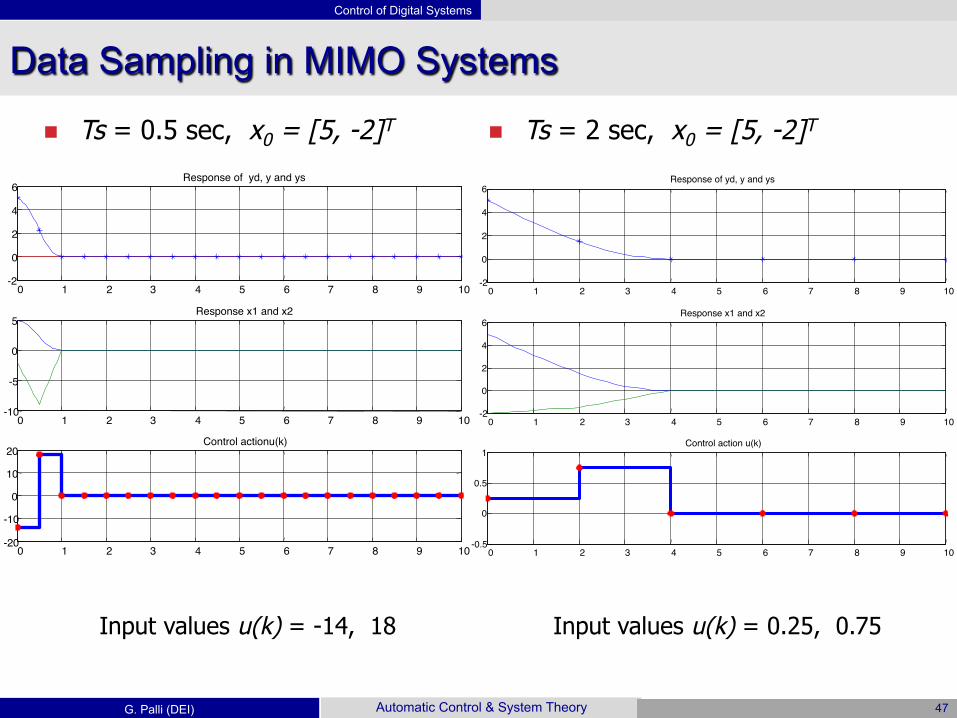
n  Ts = 0.5 sec, x0 = [5, -2]T

Input values u(k) = -14, 18

0 1 2 3 4 5 6 7 8 9 10 -2 0 2 4 6 Response of yd, y and ys

0 1 2 3 4 5 6 7 8 9 10 -10 -5 0 5 Response x1 and x2

0 1 2 3 4 5 6 7 8 9 10 -20 -10

0 10 20 Control actionu(k)

n  Ts = 2 sec, x0 = [5, -2]T

0 1 2 3 4 5 6 7 8 9 10 -2 0 2 4 6 Response of yd, y and ys

0 1 2 3 4 5 6 7 8 9 10 -2 0 2 4 6 Response x1 and x2

0 1 2 3 4 5 6 7 8 9 10 -0.5 0

0.5 1 Control action u(k)

Input values u(k) = 0.25, 0.75




n  Ts = 1 sec, x0 = [5, -2]T, square input setpoint with amplitude A = 10

0 10 20 30 40 50 60 -5 0 5

10 15 Respose of yd, y and ys

0 10 20 30 40 50 60 -10 -5 0 5

10 15 Response of x1 and x2

0 10 20 30 40 50 60 -3

-2

-1

0

1

2

3 Control action u(k)




n  If the state is not measureable, a dead-beat observer can be designed: in such an observer the state estimation error evolves with a dynamics characterized by two null eigenvalues (modes). This means that the eigenvalues of A+LC (or F+LH) are all zeros.

n  Example: design of a reduced-order dead-beat observer.

n  Recalling the design of a generic reduced-order observer in the discrete-time case: the system output directly coincides with the first q=1 components of the state.

n  Therefore, the observer dynamics is:

F

G




n  The dynamics of the dead-beat reduced-order observeris then:

it follows

and the state estimation is:

n  The transfer function G(s) of the continuous-time system is: n  The transfer function G(z) of the

corrsponding discrete-time system is:

n  The eigenvalues are imposed to be zero:




Zero-Order Hold1

Zero-Order Hold

uo To Workspace6

xhat To Workspace4

ys To Workspace3

xo To Workspace2

yd To Workspace14

y To Workspace13

t To Workspace1

In1 y

In2 u x hat

Subsystem

Pulse Generator

K*u Kups

K*u K

1 s

Integrator

Clock

K*u C.

K*u C

K*u B

K*u A

n  Simulink scheme

K*u

K*u L

-1

-1 Z

Integer Delay K*u

-1/T

2

1 In1 y

1 x hat

T/2 Z

Integer Delay1 In2 u




0 1 2 3 4 5 6 7 8 9 10 -10 -5 0 5 Andamento yd, y e ys

0 1 2 3 4 5 6 7 8 9 10 -10 -5 0 5

10 Andamento x1 e x2

0 1 2 3 4 5 6 7 8 9 10 -5 0 5

10 Azione di controllo u(k)

0 1 2 3 4 5 6 7 8 9 10 -10 -5 0 5 Andamento yd, y e ys

0 1 2 3 4 5 6 7 8 9 10 -20 -10

0 10 20 Andamento x1 e x2

0 1 2 3 4 5 6 7 8 9 10 -20 0

20 40 Azione di controllo u(k)

n  Ts = 2 sec, x0 = [5, -2]T n  Ts = 1 sec, x0 = [5, -2]T




n  Ts = 2 sec, x0 = [5, -2]T n  Ts = 1 sec, x0 = [5, -2]T

0 10 20 30 40 50 60 -5 0 5

10 15 Andamento yd, y e ys

0 10 20 30 40 50 60 -10 0

10 20 Andamento x1 e x2

0 10 20 30 40 50 60 -5

0

5 Azione di controllo u(k)

0 10 20 30 40 50 60 -5 0 5

10 15 Andamento yd, y e ys

0 10 20 30 40 50 60 -20 -10

0 10 20 Andamento x1 e x2

0 10 20 30 40 50 60 -20 -10

0 10 20 Azione di controllo u(k)



Automatic Control & System Theory 54 G. Palli (DEI)

AUTOMATIC CONTROL AND SYSTEM THEORY

CONTROL OF DIGITAL SYSTEMS

THE END

automatic control and system theory - … · control of digital systems g. palli (dei) automatic...

Documents