automatic estimating sound wave overview acoustic of p · phoneme example phoneme example phoneme...
TRANSCRIPT
Acoustic Theory of Speech Production
• Overview
• Sound sources
• Vocal tract transfer function
– Wave equations
– Sound propagation in a uniform acoustic tube
• Representing the vocal tract with simple acoustic tubes
• Estimating natural frequencies from area functions
• Representing the vocal tract with multiple uniform tubes
6.345 Automatic Speech Recognition Acoustic Theory of Speech Production 1
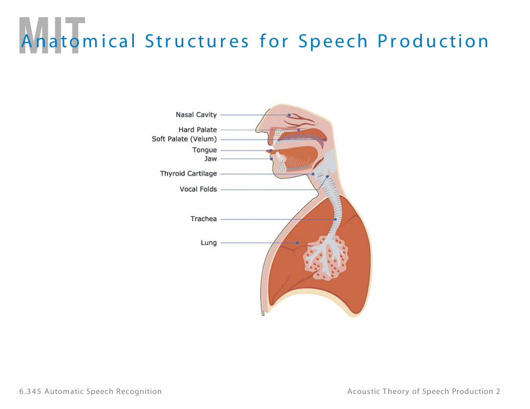
A n a to m i ca l St r u ctu r e s f o r Sp e e ch P r o d u ct i o n
6 .3 4 5 Automatic Speech Recognition Acous tic T heory of Speech Production 2
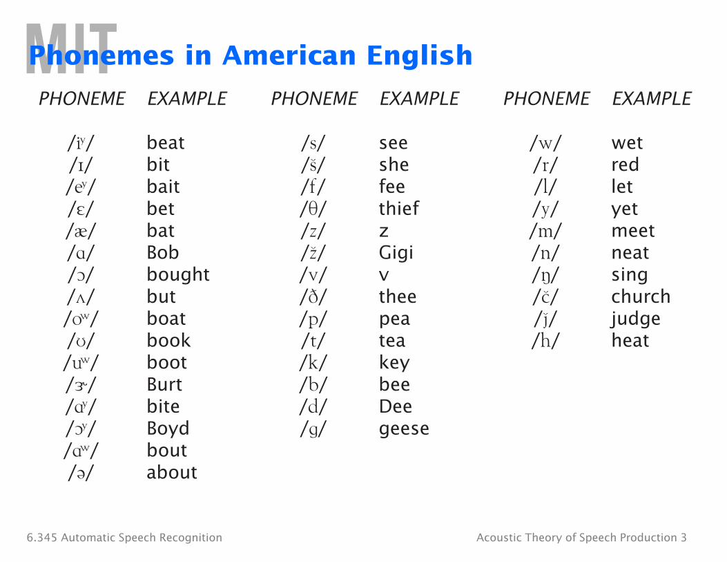
Phonemes in American English
PHONEME EXAMPLE PHONEME EXAMPLE PHONEME EXAMPLE
/i¤/ beat /I/ bit /e¤/ bait /E/ bet /@/ bat /a/ Bob /O/ bought /^/ but /o⁄/ boat /U/ book /u⁄/ boot /5/ Burt /a¤/ bite /O¤/ Boyd /a⁄/ bout /{/ about
/s/ see /w/ wet /S/ she /r/ red /f/ fee /l/ let /T/ thief /y/ yet /z/ z /m/ meet /Z/ Gigi /n/ neat /v/ v /4/ sing /D/ thee /C/ church /p/ pea /J/ judge /t/ tea /h/ heat /k/ key /b/ bee /d/ Dee /g/ geese
6.345 Automatic Speech Recognition Acoustic Theory of Speech Production 3
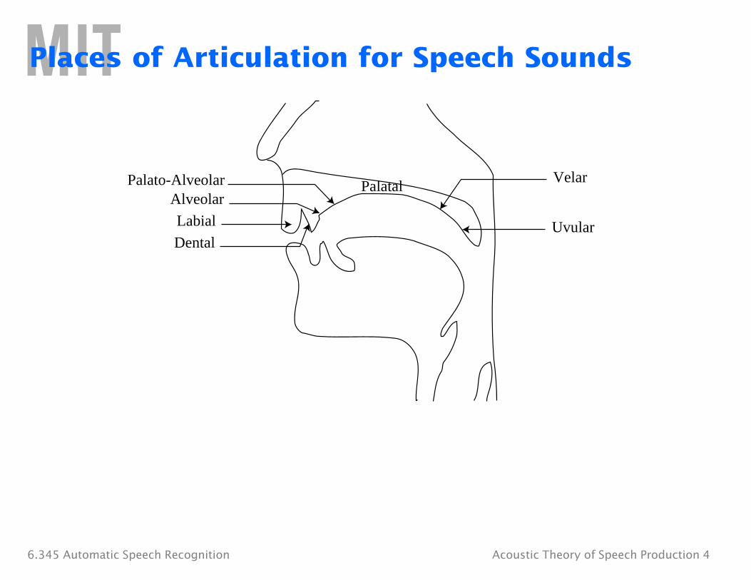
Places of Articulation for Speech Sounds
Palato-Alveolar Velar
Alveolar
Labial Uvular Dental
Palatal
6.345 Automatic Speech Recognition Acoustic Theory of Speech Production 4
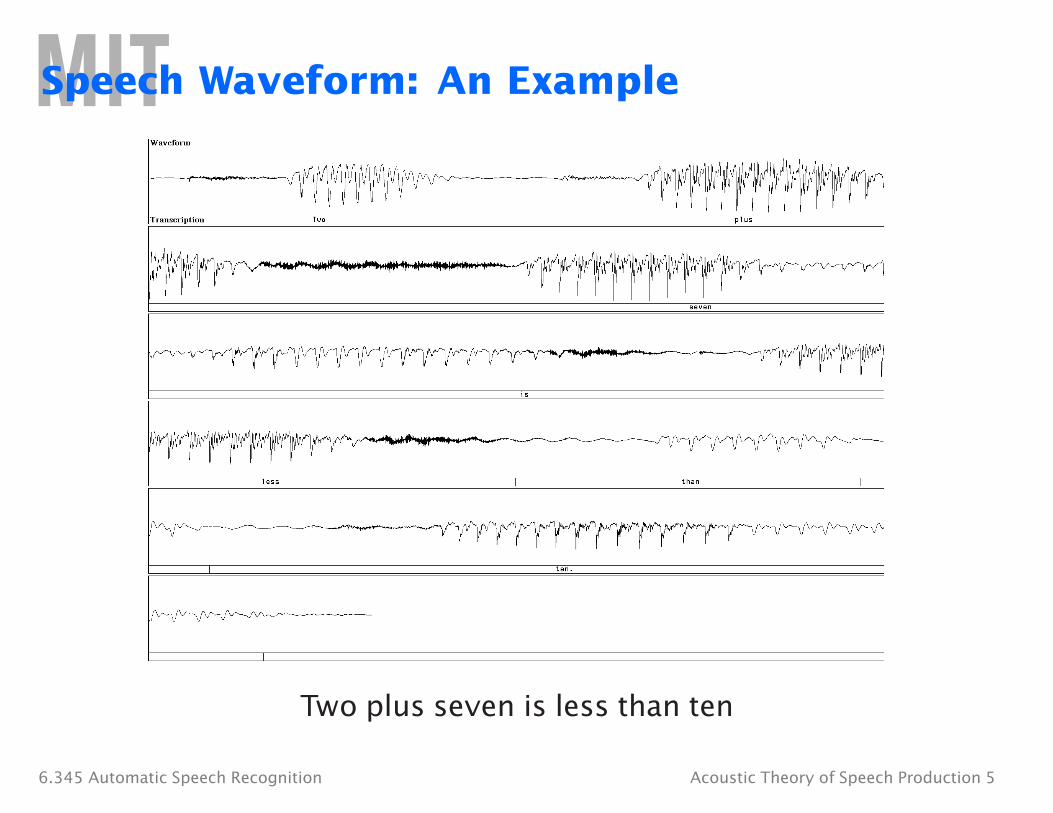
Speech Waveform: An Example
Two plus seven is less than ten
6.345 Automatic Speech Recognition Acoustic Theory of Speech Production 5
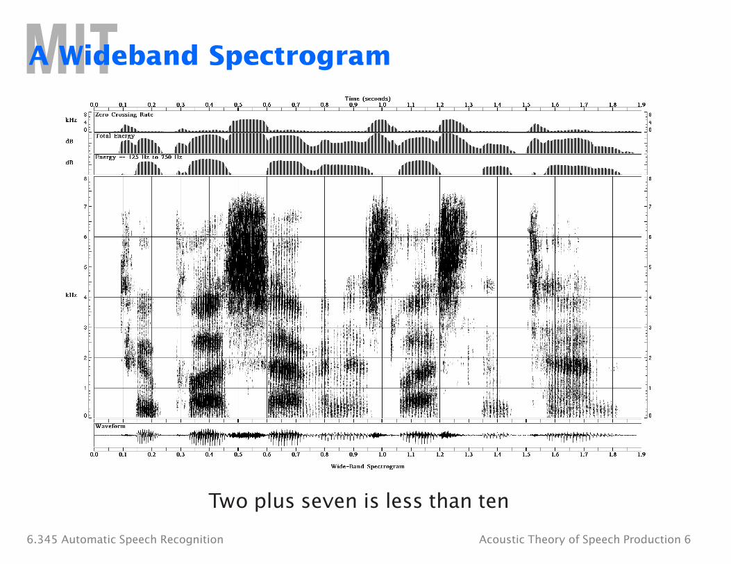
A Wideband Spectrogram
Two plus seven is less than ten
6.345 Automatic Speech Recognition Acoustic Theory of Speech Production 6
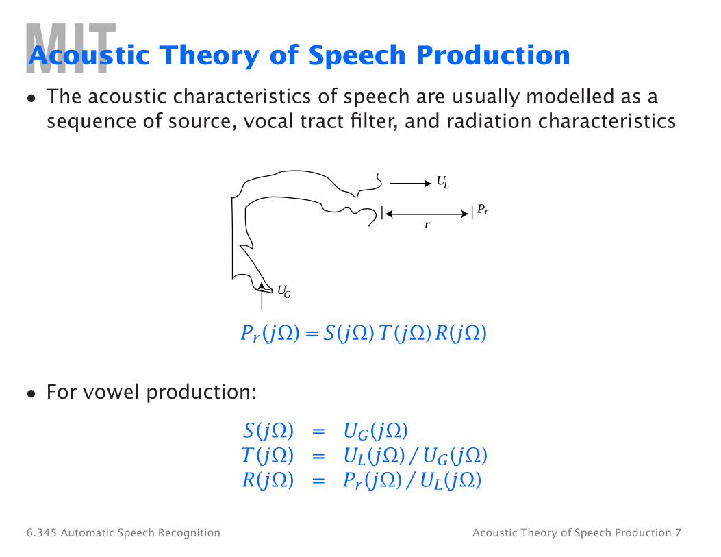
Acoustic Theory of Speech Production
• The acoustic characteristics of speech are usually modelled as a sequence of source, vocal tract filter, and radiation characteristics
UG
UL
Pr r
Pr (jΩ) = S(jΩ) T (jΩ) R(jΩ)
• For vowel production:
S(jΩ) = UG(jΩ) T (jΩ) = UL(jΩ) / UG(jΩ) R(jΩ) = Pr (jΩ) / UL(jΩ)
6.345 Automatic Speech Recognition Acoustic Theory of Speech Production 7
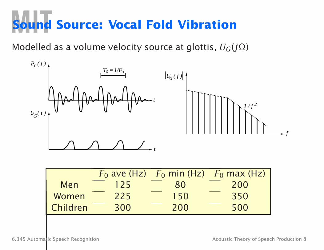
Sound Source: Vocal Fold Vibration
Modelled as a volume velocity source at glottis, UG(jΩ)
Pr ( t )
UG
( t )
T 1/Fo o =
t
t
UG ( f )
1 / f 2
f
F0 ave (Hz) F0 min (Hz) F0 max (Hz) Men 125 80 200
Women 225 150 350 Children 300 200 500
6.345 Automatic Speech Recognition Acoustic Theory of Speech Production 8
�
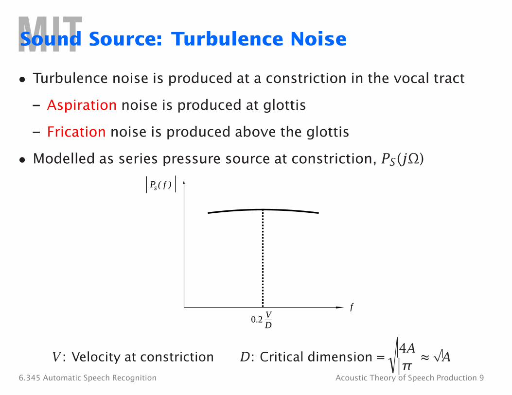
Sound Source: Turbulence Noise
• Turbulence noise is produced at a constriction in the vocal tract
– Aspiration noise is produced at glottis
– Frication noise is produced above the glottis
• Modelled as series pressure source at constriction, PS (jΩ)
P ( f )s
f
0.2 V D
4A √ V : Velocity at constriction D: Critical dimension = ≈ A
π 6.345 Automatic Speech Recognition Acoustic Theory of Speech Production 9
� �
� �
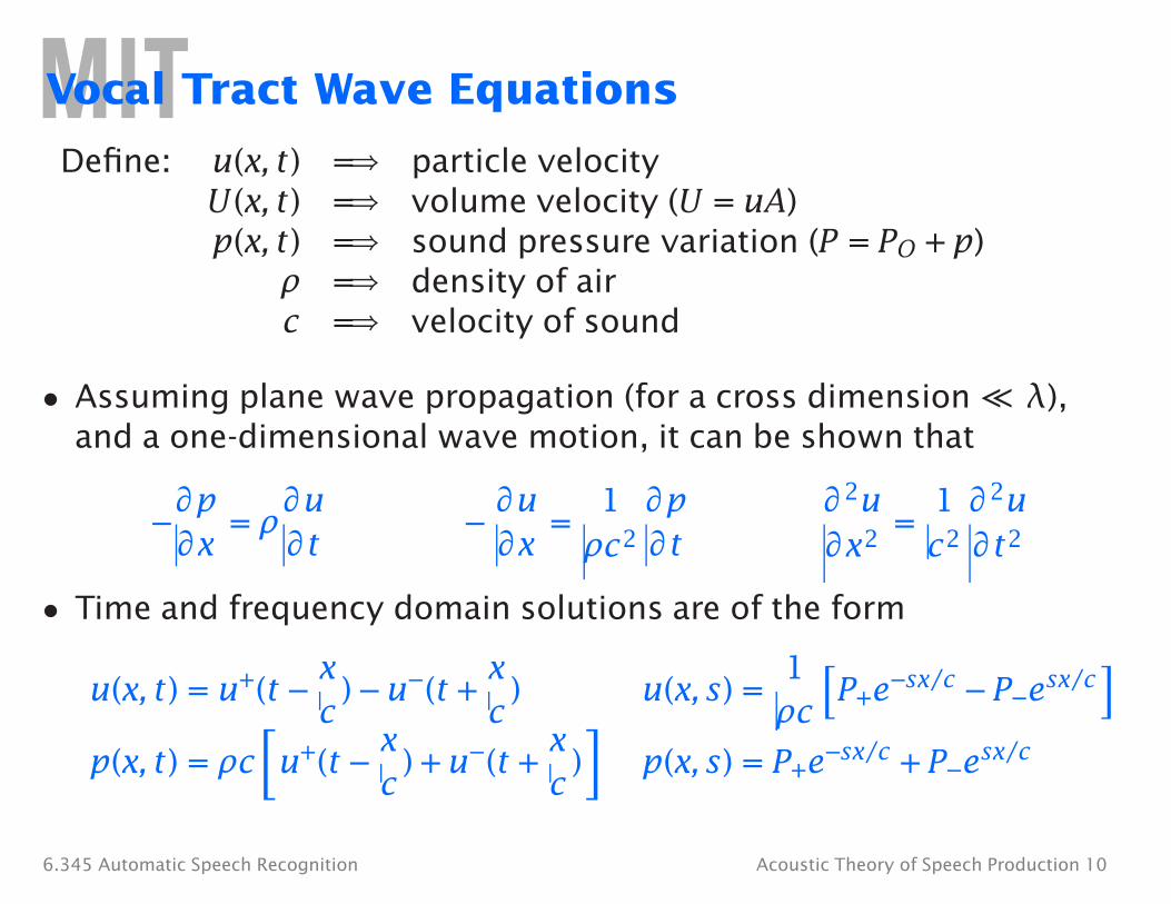
Vocal Tract Wave Equations
Define: u(x, t) =⇒ U (x, t) =⇒ p(x, t) =⇒
ρ =⇒c =⇒
particle velocityvolume velocity (U = uA)sound pressure variation (P = PO + p)density of airvelocity of sound
• Assuming plane wave propagation (for a cross dimension � λ), and a one-dimensional wave motion, it can be shown that
− ∂p
= ρ∂u −
∂u =
1 ∂p ∂2u 1 ∂2u =
∂x ∂t ∂x ρc2 ∂t ∂x2 c2 ∂t2
• Time and frequency domain solutions are of the form
u(x, t) = u+(t − x
) − u−(t + x
) u(x, s) = 1
P+e−sx/c − P−esx/c
c c ρc x x
p(x, t) = ρc u+(t − ) + u−(t + ) p(x, s) = P+e−sx/c + P−esx/c
c c
6.345 Automatic Speech Recognition Acoustic Theory of Speech Production 10
UG
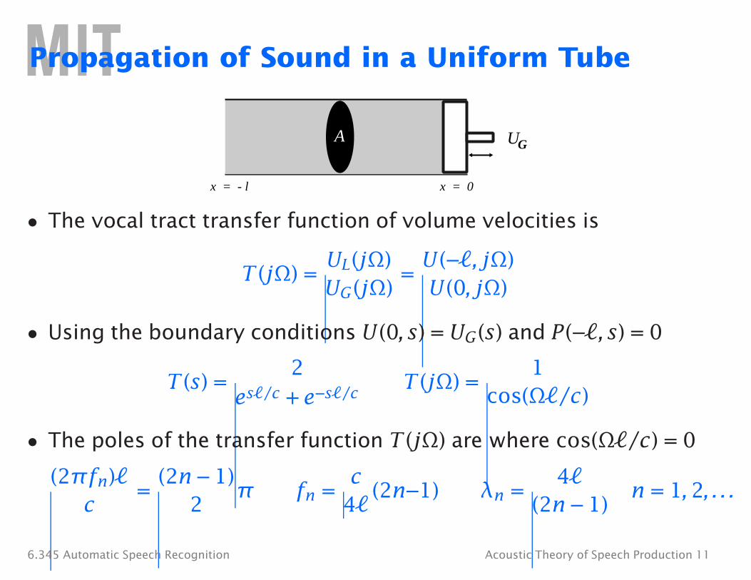
Propagation of Sound in a Uniform Tube
A
x = - l x = 0
• The vocal tract transfer function of volume velocities is
UL(jΩ) U (−�, jΩ)T (jΩ) =
UG(jΩ) =
U (0, jΩ)
• Using the boundary conditions U (0, s) = UG(s) and P(−�, s) = 0
2 1 T (s) =
es�/c + e−s�/c T (jΩ) =
cos(Ω�/c)
• The poles of the transfer function T (jΩ) are where cos(Ω�/c) = 0
4�(2πfn)� =
(2n 2 − 1)
π fn = 4 c
� (2n−1) λn =
(2n − 1) n = 1, 2, . . .
c
6.345 Automatic Speech Recognition Acoustic Theory of Speech Production 11
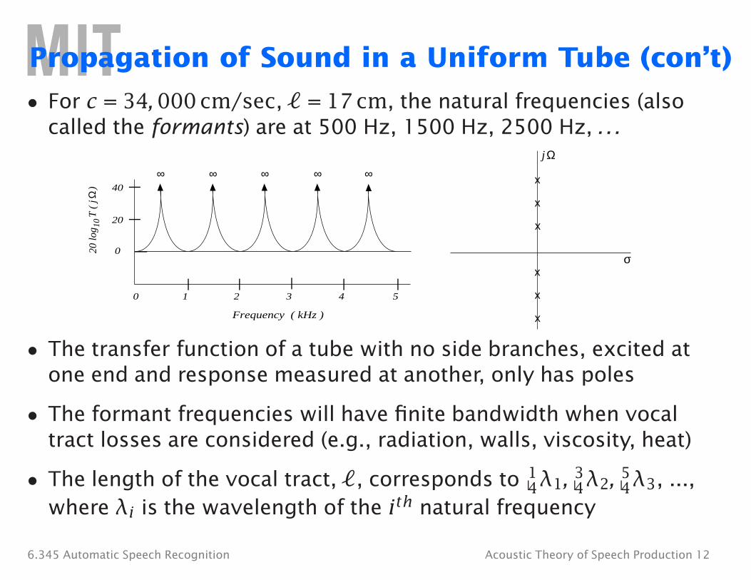
Propagation of Sound in a Uniform Tube (con’t)
• For c = 34, 000 cm/sec, � = 17 cm, the natural frequencies (also called the formants) are at 500 Hz, 1500 Hz, 2500 Hz, . . .
Ωj
x
x
x
x
x
x
∞ ∞∞∞ ∞40)
Ω
T (
j
2010
20 lo
g
0 σ
0 1 2 3 4 5
Frequency ( kHz )
• The transfer function of a tube with no side branches, excited at one end and response measured at another, only has poles
• The formant frequencies will have finite bandwidth when vocal tract losses are considered (e.g., radiation, walls, viscosity, heat)
4 λ1, 4 λ2, 4 λ3, ...,• The length of the vocal tract, �, corresponds to 1 3 5
where λi is the wavelength of the ith natural frequency
6.345 Automatic Speech Recognition Acoustic Theory of Speech Production 12
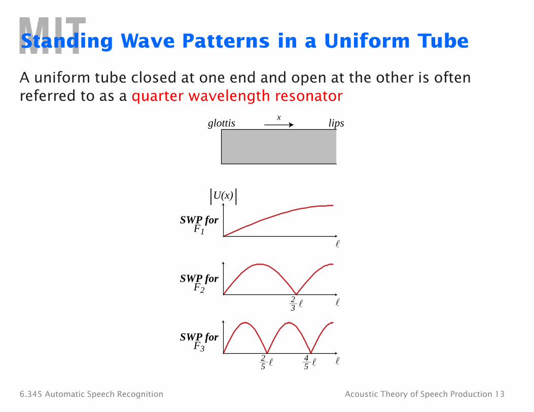
Standing Wave Patterns in a Uniform Tube
A uniform tube closed at one end and open at the other is often referred to as a quarter wavelength resonator
xglottis lips
SWP for F1
|U(x)|
SWP for F2
2 3
SWP for F3
2 4 5 5
6.345 Automatic Speech Recognition Acoustic Theory of Speech Production 13
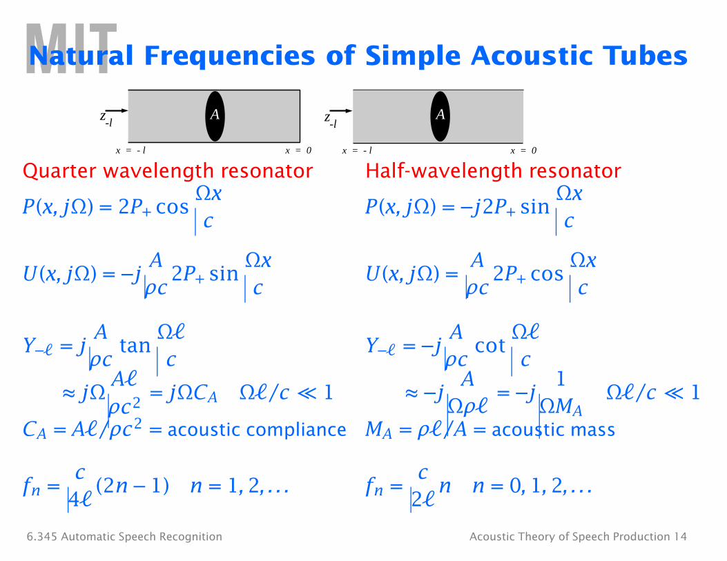
Natural Frequencies of Simple Acoustic Tubes
z-l
A z-l
A
x = - l x = 0 x = - l x = 0
Quarter wavelength resonator Half-wavelength resonator
P(x, jΩ) = 2P+ cosΩx
P(x, jΩ) = −j2P+ sin Ωx
c c
U(x, jΩ) = −jA A ρc
2P+ sinΩx
U(x, jΩ) = ρc
2P+ cosΩx
c c
ρc tan
ρc cotY−� = j
A Ω� Y−� = −j
A Ω� c c
≈ jΩA� A 1
ρc2 = jΩCA Ω�/c � 1 ≈ −j
Ωρ� = −j
ΩMA Ω�/c � 1
CA = A�/ρc2 = acoustic compliance MA = ρ�/A = acoustic mass
c cfn =
4�(2n − 1) n = 1, 2, . . . fn =
2�n n = 0, 1, 2, . . .
6.345 Automatic Speech Recognition Acoustic Theory of Speech Production 14
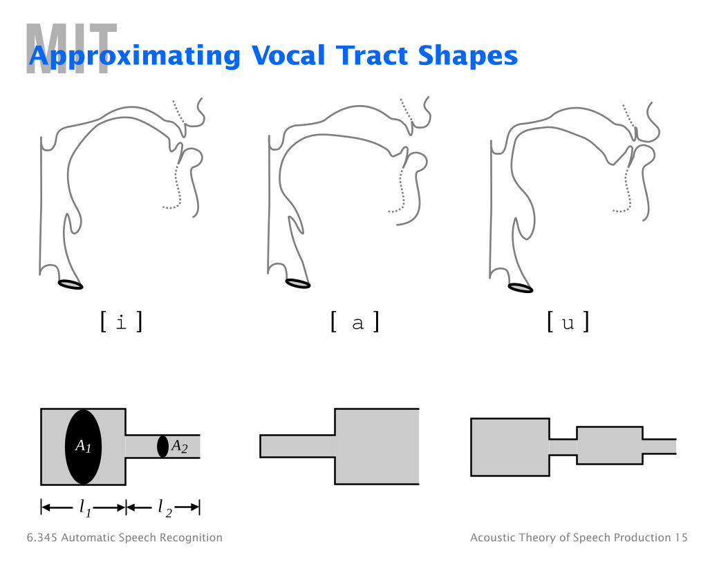
Approximating Vocal Tract Shapes
[� i� ] [ a� ] [� u� ]
A1 A2
1 l 2 l
6.345 Automatic Speech Recognition Acoustic Theory of Speech Production 15
2
1 2
l
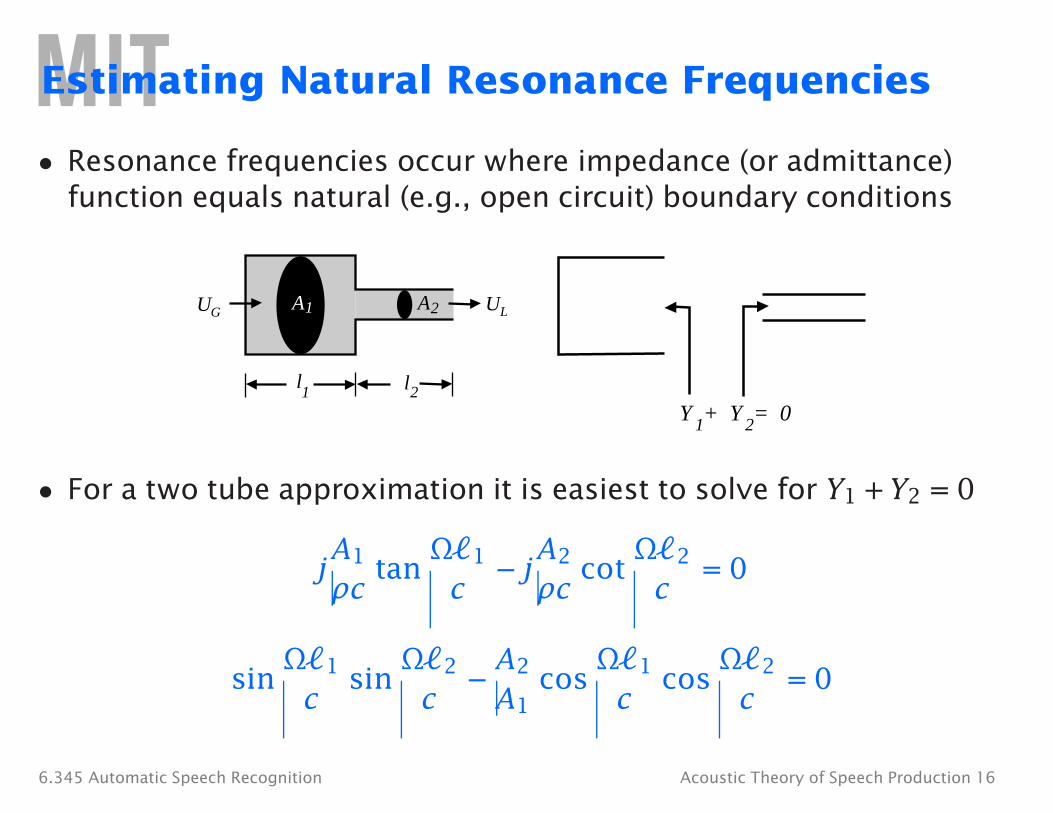
Estimating Natural Resonance Frequencies
• Resonance frequencies occur where impedance (or admittance) function equals natural (e.g., open circuit) boundary conditions
UG A1 A2 UL
1l
Y + Y = 0
• For a two tube approximation it is easiest to solve for Y1 + Y2 = 0
jA1 tan
Ω�1 −�j A2 cot Ω�2 = 0
ρc c ρc c
sin Ω�1 sin
Ω�2 −�A2 cos Ω�1 cos
Ω�2 = 0 c c A1 c c
6.345 Automatic Speech Recognition Acoustic Theory of Speech Production 16
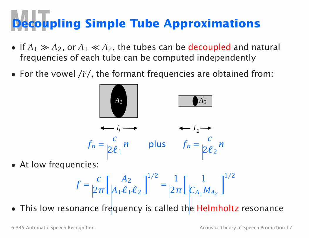
Decoupling Simple Tube Approximations
• If A1 ��A2, or A1 ��A2, the tubes can be decoupled and natural frequencies of each tube can be computed independently
• For the vowel /i¤/, the formant frequencies are obtained from:
A1 A2
1l 2l
c c fn = 2�1
n plus fn = 2�2 n
• At low frequencies: ��A2
�1/2 1 ��
1 �1/2 c
f = = 2π A1�1�2 2π CA1 MA2
• This low resonance frequency is called the Helmholtz resonance
6.345 Automatic Speech Recognition Acoustic Theory of Speech Production 17
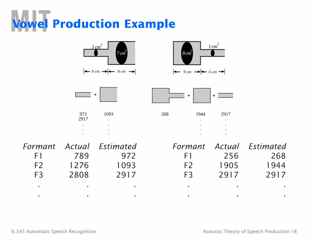
Vowel Production Example
7 cm2
1 cm2
8 cm2
1 cm2
9 cm 8 cm 9 cm 6 cm
+ + +
1093 268 1944 2917972 2917 . . .
. . . .
. . . .
. . . .
Formant Actual Estimated Formant Actual F1 789 972 F1 256 F2 1276 1093 F2 1905 F3 2808 2917 F3 2917 . . . . . . . . . .
Estimated 268
1944 2917
.
.
6.345 Automatic Speech Recognition Acoustic Theory of Speech Production 18
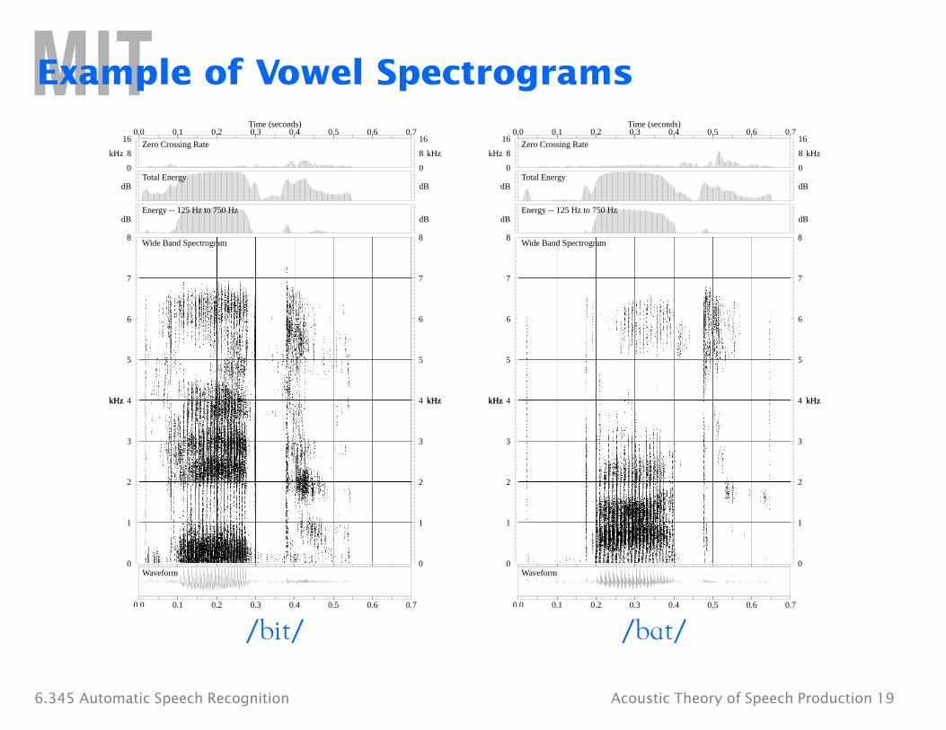
Example of Vowel Spectrograms
kHz kHz
Wide Band Spectrogram
kHz kHz
0
1
2
3
4
5
6
7
8
0
1
2
3
4
5
6
7
8
Time (seconds)0.0 0.1 0.2 0.3 0.4 0.5 0.6 0.7
kHz kHz
0 0
8 8
16 16Zero Crossing Rate
dB dBTotal Energy
dB dBEnergy -- 125 Hz to 750 Hz
Waveform
0.0 0.1 0.2 0.3 0.4 0.5 0.6 0.7
kHz kHz
Wide Band Spectrogram
kHz kHz
0
1
2
3
4
5
6
7
8
0
1
2
3
4
5
6
7
8
Time (seconds)0.0 0.1 0.2 0.3 0.4 0.5 0.6 0.7
kHz kHz
0 0
8 8
16 16Zero Crossing Rate
dB dBTotal Energy
dB dBEnergy -- 125 Hz to 750 Hz
Waveform
0.0 0.1 0.2 0.3 0.4 0.5 0.6 0.7
/bit/ bat/
6.345 Automatic Speech Recognition Acoustic Theory of Speech Production 19
/
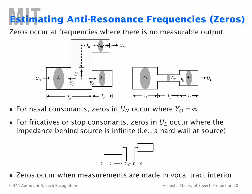
Estimating Anti-Resonance Frequencies (Zeros)Zeros occur at frequencies where there is no measurable output
UN
UG Ap Ao
An
Yp Yo
Yn
n l
Ab Ac Af P s UL
lp lo l b l c l f
• For nasal consonants, zeros in UN occur where YO = ∞
• For fricatives or stop consonants, zeros in UL occur where the impedance behind source is infinite (i.e., a hard wall at source)
Y = 0 Y + Y = 01 3 4
• Zeros occur when measurements are made in vocal tract interior 6.345 Automatic Speech Recognition Acoustic Theory of Speech Production 20
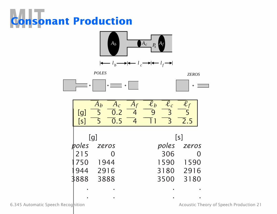
Consonant Production
Ab Ac AfPs
l b l c l f
POLES ZEROS
+ + + +
Ab Ac Af �b �c �f
[g] 5 0.2 4 9 3 5 [s] 5 0.5 4 11 3 2.5
[g] [s] poles zeros poles zeros 215 0 306 0
1750 1944 1590 1590 1944 2916 3180 2916 3888 3888 3500 3180
. . . .
. . . .6.345 Automatic Speech Recognition Acoustic Theory of Speech Production 21
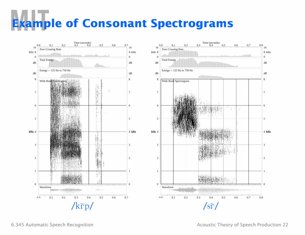
Example of Consonant Spectrograms
kHz kHz
Wide Band Spectrogram
kHz kHz
0
1
2
3
4
5
6
7
8
0
1
2
3
4
5
6
7
8
Time (seconds)0.0 0.1 0.2 0.3 0.4 0.5 0.6 0.7
kHz kHz
0 0
8 8
16 16Zero Crossing Rate
dB dBTotal Energy
dB dBEnergy -- 125 Hz to 750 Hz
Waveform
0.0 0.1 0.2 0.3 0.4 0.5 0.6 0.7
kHz kHz
Wide Band Spectrogram
kHz kHz
0
1
2
3
4
5
6
7
8
0
1
2
3
4
5
6
7
8
Time (seconds)0.0 0.1 0.2 0.3 0.4 0.5 0.6 0.7 0.8
kHz kHz
0 0
8 8
16 16Zero Crossing Rate
dB dBTotal Energy
dB dBEnergy -- 125 Hz to 750 Hz
Waveform
0.0 0.1 0.2 0.3 0.4 0.5 0.6 0.7 0.8
/ki¤ p/ si¤ /
6.345 Automatic Speech Recognition Acoustic Theory of Speech Production 22
/
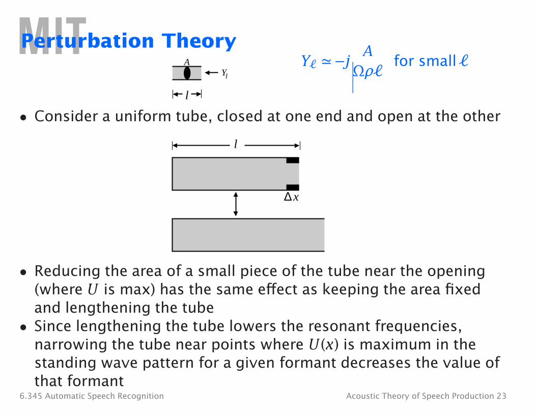
A Ωρ�
A Y� � −jYl
Perturbation Theory for small �
l
• Consider a uniform tube, closed at one end and open at the other
l
Δ x
• Reducing the area of a small piece of the tube near the opening (where U is max) has the same effect as keeping the area fixed and lengthening the tube
• Since lengthening the tube lowers the resonant frequencies, narrowing the tube near points where U (x) is maximum in the standing wave pattern for a given formant decreases the value of that formant
6.345 Automatic Speech Recognition Acoustic Theory of Speech Production 23
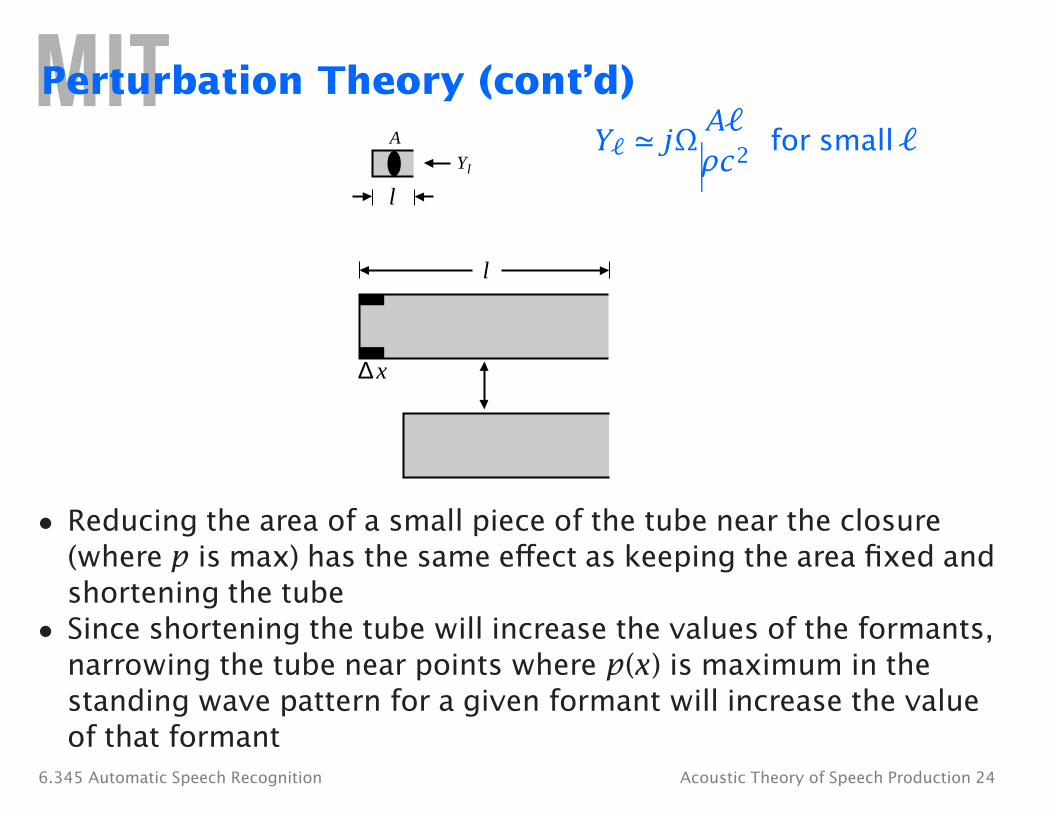
A� Perturbation Theory (cont’d)
A Y� � jΩ ρc2
for small � Yl
l
l
Δ x
• Reducing the area of a small piece of the tube near the closure (where p is max) has the same effect as keeping the area fixed and shortening the tube
• Since shortening the tube will increase the values of the formants, narrowing the tube near points where p(x) is maximum in the standing wave pattern for a given formant will increase the value of that formant
6.345 Automatic Speech Recognition Acoustic Theory of Speech Production 24
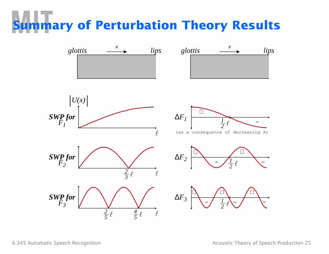
Summary of Perturbation Theory Results
xglottis lips
SWP for F1
|U(x)|
SWP for F2
2 3
SWP for F3
2 4 5 5
xglottis lips
Δ F1 1 2
+
−
(as a consequence of decreasing A)
Δ F2 1 2
+ +
− −
Δ F3 1 2
−
++
−
+
−
6.345 Automatic Speech Recognition Acoustic Theory of Speech Production 25
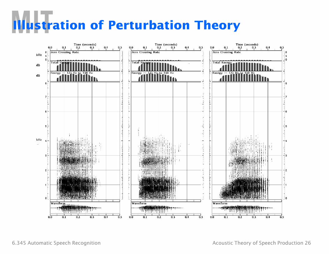
Illustration of Perturbation Theory
6.345 Automatic Speech Recognition Acoustic Theory of Speech Production 26
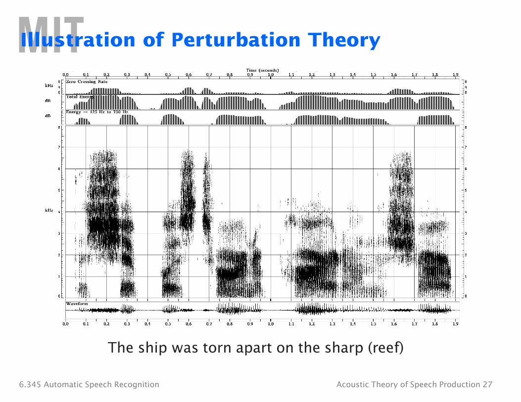
Illustration of Perturbation Theory
The ship was torn apart on the sharp (reef)
6.345 Automatic Speech Recognition Acoustic Theory of Speech Production 27
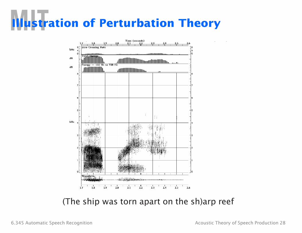
Illustration of Perturbation Theory
(The ship was torn apart on the sh)arp reef
6.345 Automatic Speech Recognition Acoustic Theory of Speech Production 28
�
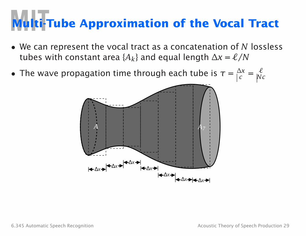
Multi-Tube Approximation of the Vocal Tract
• We can represent the vocal tract as a concatenation of N lossless tubes with constant area {Ak}�and equal length Δx = �/N
• The wave propagation time through each tube is τ = Δx = Ncc
A A7
Δx
ΔxΔx Δx
Δx Δx
Δx
6.345 Automatic Speech Recognition Acoustic Theory of Speech Production 29
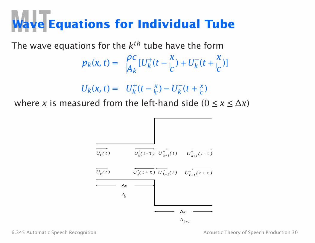
Wave Equations for Individual Tube
The wave equations for the kth tube have the form ρc x Ak
k (t −�x ) + U −�
c pk(x, t) = [U +
k (t + )] c
Uk(x, t) = U + c ) −�U −�
c )k (t −�x k (t + x
where x is measured from the left-hand side (0 ≤�x ≤�Δx)
+ + + +Uk ( t ) Uk( t - τ ) U k+1
( t ) U k+1
( t - τ )
- - - -Uk ( t ) U k( t + τ ) U k+1( t ) U
k+1( t + τ )
Ak
Δx
Δx
A k+1
6.345 Automatic Speech Recognition Acoustic Theory of Speech Production 30
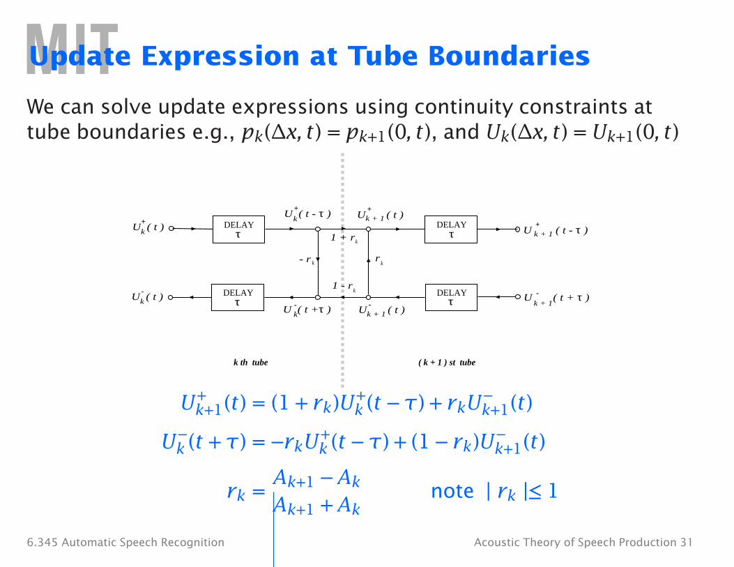
Update Expression at Tube Boundaries
We can solve update expressions using continuity constraints at tube boundaries e.g., pk(Δx, t) = pk+1(0, t), and Uk(Δx, t) = Uk+1(0, t)
+ k + 1 U+
k + 1 U-
kU τ ) -
k U τ )
+
1 - r
1 + rk
k
rk k - r
τ DELAY
τ DELAY
τ DELAY
τ DELAY
k th ( k + 1 ) st
k (t −�τ) + rkU −�
( t )
( t ) ( t +
( t -
tube tube
+Uk ( t ) U k + 1 ( t - τ )
- -Uk ( t ) U k + 1
( t + τ )
Uk ++1(t) = (1 + rk)U +
k+1(t)
Uk −(t + τ) = −rkUk
+(t −�τ) + (1 −�rk)U −�k+1(t)
rk = Ak+1 −�Ak note |�rk |≤�1 Ak+1 + Ak
6.345 Automatic Speech Recognition Acoustic Theory of Speech Production 31
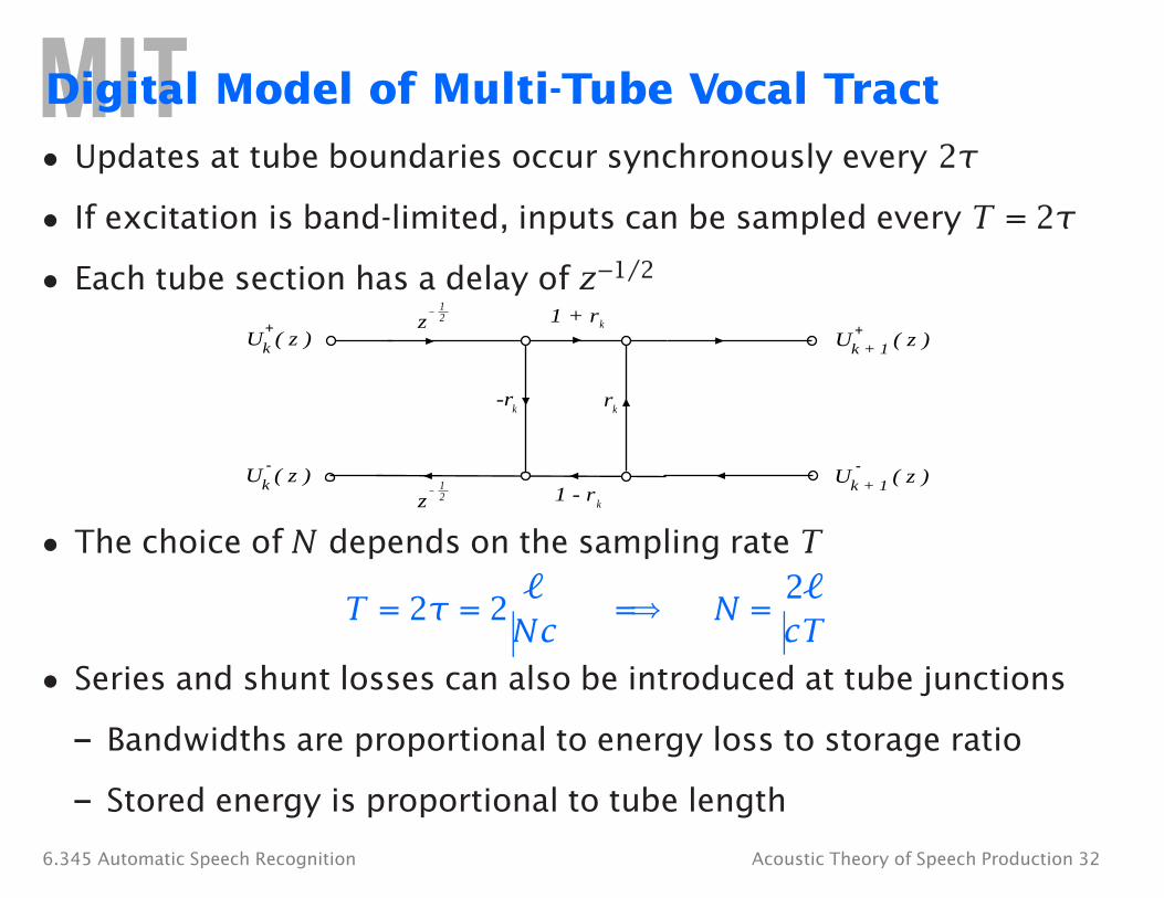
Digital Model of Multi-Tube Vocal Tract
• Updates at tube boundaries occur synchronously every 2τ
• If excitation is band-limited, inputs can be sampled every T = 2τ
• Each tube section has a delay of z−1/2 1
+ z 2 1 + rk +Uk ( z )
kr
1
k -r
Uk + 1 ( z )
- -Uk ( z ) Uk + 1 ( z )
z 2 1 - rk
• The choice of N depends on the sampling rate T
T = 2τ = 2 �
=⇒� N =2�
Nc cT
• Series and shunt losses can also be introduced at tube junctions
– Bandwidths are proportional to energy loss to storage ratio
– Stored energy is proportional to tube length
6.345 Automatic Speech Recognition Acoustic Theory of Speech Production 32
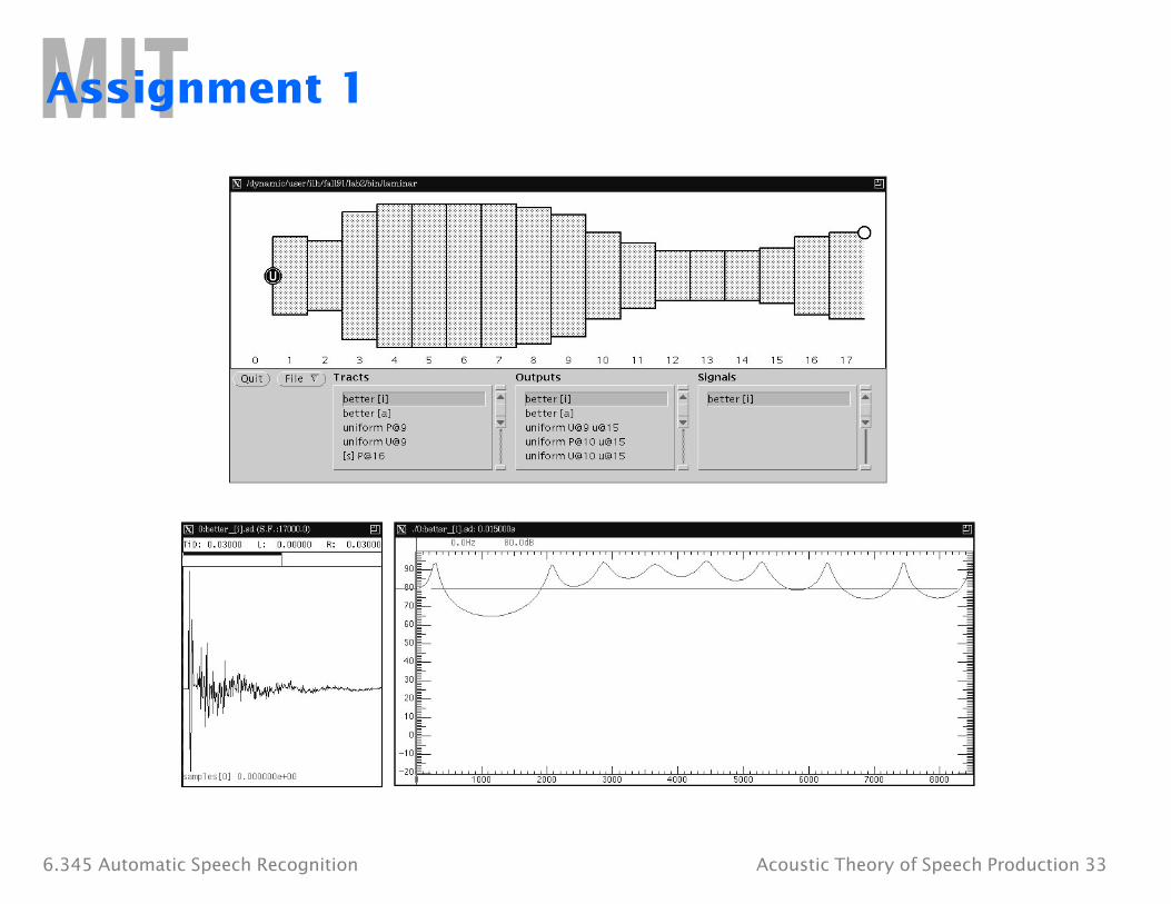
Assignment 1
6.345 Automatic Speech Recognition Acoustic Theory of Speech Production 33
References
• Zue, 6.345 Course Notes
• Stevens, Acoustic Phonetics, MIT Press, 1998.
• Rabiner & Schafer, Digital Processing of Speech Signals, Prentice-Hall, 1978.
6.345 Automatic Speech Recognition Acoustic Theory of Speech Production 34