automatic gain control for a small portable ultrasound device
TRANSCRIPT

Xk; rhap uhk;
Automatic Gain Control for a Small Portable Ultrasound Device by
Sripriya Natarajan
Submitted to the Department of Electrical Engineering and Computer Science in Partial Fulfillment of the Requirements for the Degree of Master of Engineering in Electrical
Engineering and Computer Science
at the Massachusetts Institute of Technology
May 23, 2001
Copyright 2001 Sripriya Natarajan. All rights reserved.
The author hereby grants to M.I.T. permission to reproduce and distribute publicly paper and electronic copies of this thesis and to grant others the right to do so.
Author_______________________________________________________ Department of Electrical Engineering and Computer Science
July 9, 2001
Certified by____________________________________________________ Martha L. Gray Thesis Supervisor
Accepted by___________________________________________________
Arthur C. Smith Chairman, Department Committee on Graduate Theses

Automatic Gain Control for a Small Portable Ultrasound Device
Sripriya Natarajan
Department of Electrical Engineering and Computer Science, Masschusetts Institute of Technology,
Cambridge, MA
Imaging Systems Division, Healthcare Solutions Group,
Agilent Technologies Andover, MA
Abstract Among the recent innovations in ultrasound is a new portable cardiac ultrasound device being developed at Agilent Technologies’s Healthcare Solutions Group. Such a device, because of its size, can be used in many more locations than a traditional ultrasound machine, and thus potentially by many people without the same extent of training as a cardiologist or sonographer. To facilitate this type of usage, the device requires an easy-to-learn user interface, incorporating simplifying features such as automatic gain control (AGC). This project developed and evaluated prototype, real-time AGC algorithms for 2D cardiac ultrasound, implemented in software. A view-based AGC algorithm was first considered, and shown to be unsuccessful. The second AGC algorithm considered has two components: the first is a classification component that designates blocks of acoustic data as consisting primarily of blood, ordinary tissue or specular tissue samples; the second component adjusts the 2D gains such that the brightness of the image is appropriate for the given classifications. Several versions of this classification-based AGC algorithm were qualitatively evaluated by clinical specialists. Preliminary results show that some of these algorithms produced images of a quality similar to that of images produced by an experienced sonographer using a device with manual gain controls, although these AGC algorithms are not very aggressive in their alteration of gain settings from the preset values. The results also suggest that even experienced clinical specialists prefer the convenience of automatic gain control over the precision of manual gain control for a screening device.

Om Sai Ram
Table of Contents
1. Introduction and Background ..........................................................................................1
2. Feasibility of a View-Matching Algorithm for AGC ....................................................20
3. Correlating Mean and Blood/Tissue Composition .......................................................40
4. Correlating Variance and Blood/Tissue Composition..................................................56
5. Classification-Based AGC Algorithms...........................................................................67
6. Characterization of Classification-Based AGC Algorithms ........................................79
7. Clinical Evaluations of Classification-Based AGC Algorithms...................................87
8. Conclusions and Further Work....................................................................................110
References.............................................................................................................................116
Acknowledgements ..............................................................................................................118

1
Om Sai Ram
1. Introduction and Background 1.1. Introduction to Medical Ultrasonic Imaging and Time Gain
Compensation
Two-dimensional diagnostic medical ultrasound is a non-invasive, real-time imaging
modality that allows clinicians to view the internal anatomical structures and motion of a
patient by transmitting sound waves, at frequencies above the audible range for humans,
into the body and analyzing the reflections that come back. In a typical ultrasound
system, a transducer sends out ultrasound pulses and receives their echoes, which are
then processed to produce a screen image of the targeted anatomy (Karrer and Dickey,
1983).
Fig. 1-1. Diagram of the geometry of an ultrasound sector of data. Each sample has an acoustic value measuring the echo that returned from the location corresponding to the sample.

2
The strength of these echoes is proportional to the incident wave’s energy and is also a
function of the reflector’s structural properties. Typically, a transducer shoots beams of
ultrasound along different lines of sight. The direction of each consecutive line is
incremented by some constant dθ so that ultimately a sector of data is captured (see Fig.
1-1). There is an implicit, transducer-dependent thickness to this sector, since one cannot
interrogate an infinitely thin slice of the body. Echoes from deeper in the body take a
longer time to return to the transducer; by taking this time delay into account, the
received signal can be decomposed into the different echoes that were returned from
different depths along the line. After digitization, the acoustic data for one image
consists of a polar-coordinate, two-dimensional array of s samples per line for N lines.
(Typically, N is on the order of a hundred, and s is on the order of a few hundred.) These
samples are then scan converted to generate pixel values for the rectangular coordinate
system of the display. This process is repeated many times a second so that the user can
perceive the motion of the heart.
(a) (b)
Fig. 1-2. Good quality typical cardiac ultrasound images. (a) Parasternal long axis view. (b) Apical four chamber view. Dark areas indicate blood-filled cavities, and bright areas indicate echolucent tissue.

3
A gain factor must be applied, in part before A/D conversion (front end) and in part after
A/D conversion (back end), to each of the pre-scan-conversion acoustic samples to create
images of adequate quality that accurately represent the target anatomy. Fig.1-2 shows
two good cardiac ultrasound images. The dark regions correspond to blood-filled
chambers of the heart, and the bright features correspond to the echolucent tissue of the
heart, including the heart wall and valves. The applied gain should be high enough that
the tissue is smooth and the valves appear well-defined, but not so high that the dark
chambers are filled with bright “clutter.” Fig. 1-3 shows examples of poor images
generated with improper gain settings. In addition, the soft tissue should be displayed
with similar, moderate gray pixel levels. To achieve this uniformity, the gain applied to
each sample may be different because energy losses are not constant over space or time.
Various propagation effects cause the signal to be attenuated differently depending on the
path of the sound wave and the distance it has traveled.
(a) (b)
Fig. 1-3. Cardiac ultrasound images generated with poor gain settings. (a) Parasternal long axis view generated with low gain settings. Note how the valves are not sharply delineated. (b) Apical four chamber view generated with high gain settings. Note that the chamber is filled with bright clutter, making it appear similar to tissue.

4
Time gain compensation (TGC) refers to the determination and application of a gain
profile depending on the distance that an ultrasound wave has traveled. Attenuation
increases with distance traveled. Since a sound wave travels to some point in the body
and is reflected back, the distance traveled is proportional to the depth of a sample by a
factor of 2. The speed of sound in the human body ranges from 1450 m/s in fat to 1580
m/s in blood and tissue (Rose, et. al. 20). If one approximates this speed to be a constant,
then the distance traveled by the waves are approximately proportional to the time of
propagation (thus, time gain compensation). Deeper echoes are weaker not only because
the received signal has attenuated more, but also because the incident pulse is weaker
when it hits the tissue. Thus, samples at a greater depth (far field) must have more gain
applied to them than shallower ones (near field) to normalize the returning echo values.
The transducer, or probe, design parameters also significantly affect the degree of
attenuation reflected in the value of a given sample. The strength of the returning echoes
is proportional to the power of the incident beam sent by the transducer. Attenuation
increases with higher frequency; thus the center frequency of the spectrum of a beam of
ultrasound shifts down as the beam goes deeper, as the amplitudes of the higher
frequencies fall off faster than those of the lower frequencies. This phenomenon, known
as beam softening, leads to a weaker incidence beam at greater depths than would be
predicted by distance attenuation alone. Variations in the beam width affect the
incidence level of the sound wave and thus the intensity of the returning signal
(O’Donnell, 1983). The temperature of the transducer, an indicator of incidence power,
is another factor used to determine the gains. A “rolloff effect” is caused by differences

5
in beam focusing; beams are best focused at an angle of 0, and as the line of sight travels
to the left or right, the signal strength falls. Corrections for these physical and
mechanical factors are often hard-coded into the control system, with specific profiles for
each transducer.
These static limitations are further complicated by the fact the composition of the human
body is not homogeneous. Different types of tissues have different attenuation
coefficients and acoustic impedences. Pathologies, such as tumors and lesions, also have
very different attenuation coefficients compared to healthy tissue. In addition, fluids,
such as the blood in the human vasculature, have attenuation characteristics dramatically
different from tissue. Another factor to consider is the specular reflection of the sound
waves at boundaries between different composition types. For example, the air-filled
lung has a low acoustic impedence value of 0.26 x 10⁻⁶ kg/m2s, whereas muscular cardiac
tissue has an acoustic impedence value of 1.73 x 10⁻⁶ kg/m2s; so as a sound wave passes
from tissue to lung, more energy is reflected than is transmitted, resulting in a specular
reflection artifact (Hussey 20). Thus, although the lung is very deep in the field when
imaging the heart, the echo samples from it often need less gain than reflections off
myocardium in the mid-field. In cases where the specular reflection is caused by an
irregularity in the tissue, such as a tumor, the specular reflection itself causes an overly
bright echo, but since so much energy has been reflected, the power of incidence at
depths beyond the reflection is significantly reduced, causing the appearance of a dark
shadow below the boundary.

6
In most commercial systems, the user is allowed to manipulate gain settings for different
depth bands, and sometimes even for lateral bands, to adjust for these complicated
effects. The user settings are interpolated to create a smooth gain profile for the image.
This manual gain correction is combined with the hard-coded mechanical gain
adjustments to achieve gain profiles that produce acceptable images. A chief drawback
to manual TGC is the lack of a rational approach to determining the right profile; it is
simply trial and error until the user sees an image he or she likes. Thus, the user has to
have significant expertise to produce an image of good diagnostic quality. Since the
settings are subjective, an image is not easily reproducible by another sonographer. The
more lateral and radial bands that can be adjusted independently, the more complex the
user interface becomes. Even with several bands in either direction, however, the
resolution of control is not always enough; if tissue and fluid are in the same zone,
artifacts occur. If too little gain is applied to a subset of samples in a zone, shadows
appear in the image; if too much gain is applied, bright spots arise. Thus, the
automatization of TGC can potentially improve both the simplicity and quality of the
current methods.
1.2. New Portable Ultrasound Device
A new portable cardiac ultrasound device being developed at Agilent Technologies
provides the ideal basis for developing an automatic gain control (AGC) system. This
ultrasound device has a very different use model than traditional ultrasound machines. It
is to be used primarily as a screening tool, not chiefly by sonographers and cardiologists,
but by other medical professionals who are not extensively trained in ultrasound imaging.

7
To augment the simplicity of the user interface and minimize the amount of training
required for the effective use of the device, it would be beneficial to automate the manual
gain controls. The widespread use of the machine also begs consistency among images
so that users can learn to interpret them with ease. In addition, since the device is a
screening tool rather than a diagnostic tool, it will only be used for one to two minutes
per study. If just 30 seconds are spent only on setting gain controls, upto a third of the
study time could be spent on simply adjusting system parameters for use. AGC would
minimize this setup time overhead, and greatly benefit the device users.
The device’s use model also makes it a good candidate for a successful practical
implementation of AGC. A screening tool’s image quality requirements are not as strict
as those of a high-performance diagnostic ultrasound machine, so it is easier to produce
acceptable output images for this device than for a traditional ultrasound scanner.
Currently, the device has only two manual gain controls, one to adjust the overall gain of
the image and one to adjust the near field gain, which affects approximately the top two-
thirds of the image, as opposed to the 8 or more controls on a high performance system.
The low granularity of the current gain controls make it more likely that orginal image
quality can be matched by an AGC system. These considerations motivate this
investigation of the feasibility of implementing AGC for this ultrasound device.

8
1.3. Related Work
1.3.1. Survey of Previous Investigations
There have been several investigations into AGC and adaptive TGC in the past thirty
years. Many varied approaches have been taken to move towards the goal of AGC.
Some have based their solutions on mathematical models, while others have used
physiological reasoning to develop their algorithms. Some implementations have relied
purely on circuit feedback techniques, while others designs, especially those including a
statistical analysis of the data, have incorporated software control in their designs. The
range of approaches that have been tried speaks to both the problem’s difficulty and its
interest.
Many approaches have made the assumption that the end goal is a uniform mean
brightness. One of the earliest prototype AGC systems used analog feedback circuitry to
use the average values of the earlier data on a line to control the gain for subsequent
times on the line (McDicken, et. al., 1974). At Stanford University, researchers
elaborated on this idea by maintaining the average values at discrete bands of depth for
an image’s worth of lines, in order to improve the stability of the AGC system's response.
Averages for eight depth bands were maintained using analog circuitry, and these values
were smoothed to produce a gain function based on depth (DeClercq and Maginness,
1975).
This latter approach is reminiscent of manual gain control, since both adjust gain on a
band by band basis, and interpolate these values to define the gain profile. The theme of

9
mimicking the user’s behavior is recurrent in the design of AGC systems. A patent
assigned to Elsint, Ltd. of Israel, describes feedback circuitry for an AGC system
designed to keep intensity vs. time functions relatively flat, which operates on bands of
data (Inbar and Delevy, 1989). For a short period during the mid-1980’s, an AGC feature
based on a similar feedback mechanism was incorporated into the SKI 4500, a
commercial cardiac ultrasound system manufactured by SmithKline Instruments, Inc.
A patent taken out by General Electric Company describes an AGC system that also tries
to imitate user control by processing data independently in lateral and radial bands. This
system is unique from the others in that it attempts to filter out noise as well as equalize
the acoustic data means across bands. It includes a noise model for the entire ultrasound
processing chain, from the beamformer all the way through the video processor and uses
this model to calculate the noise at each sample, given the current ultrasound system
parameters. If enough sample values in a lateral or radial band are above their respective
noise floors, a gain is applied to bring that band’s mean to a pre-determined optimal
level. Otherwise, noise is suppressed by deamplifying the acoustic values in the band
(Mo, 2000).
Other approaches have considered the entire image’s statistics to perform AGC. One
method uses two gain functions, both smoothing functions that try to bring all pixels to a
mid-gray level. One function, F(x), compares the value of a sample at depth x to several
adjacent sample values on a given scan line. The other function, G(x), compares the
sample at depth x to all the other values in the entire image. The final gain is determined

10
by combining the output of the two functions, weighing F(x) by β and G(x) by (1 - β).
The value of the parameter β is dependent on the function values themselves. If value of
the local function F(x) is greater than the value of the global function G(x), then the
sample is probably in an anechoic region, which should be dark. Thus, β is set to zero,
and the smaller of the two gain values is used. Otherwise, the applied gain is calculated
by averaging F(x) and G(x) equally; i.e., β = 0.5 (Pye, et. al., 1992).
The methods described so far all have aimed explicitly to have a uniform mean
brightness. An alternative method is based on segmentation of acoustic samples, and
applying a different gain to each category of sample. The inventors of rational gain
compensation for cardiac ultrasound justify this approach physiologically; they
categorize samples into myocardium, blood and chest wall. Since these three
composition types have different attenuation characteristics, different gain values are
applied to each type of sample. The method uses current backscatter values to guess at
the composition type of a sample, and also takes into consideration the composition type
of a fixed number of previous contiguous samples along a line, to reduce noise. Although
this method is fairly effective at adaptive gain control, it is not wholly automatic; it
requires that the user set a threshold value to control the classification of samples, and
performance is very sensitive to this threshold value (Melton and Skorton, 1983). The
path-dependent attenuation correction (PDAC) algorithm, is similar, using image
statistics and user-defined thresholds to determine if a sample is myocardium, blood or
chest wall (Pincu, et. al., 1986).

11
One related approach also includes automated threshold selection for segmentation. This
method creates a histogram of the acoustic data along one scan line, and determines the
most frequent acoustic value, A (the location of the peak of the histogram). A lower
threshold is set at A – A/2 and an upper threshold is set at A + A/2. The samples are
segmented into those with values below the lower threshold, between the two thresholds,
and above the upper threshold. As in the other segmentation algorithms, a different gain
is applied to each category of samples. These gain coefficients themselves are
determined from the sample values in each category. The process is iterated until the
standard deviation of the histogram does not change significantly (O’Donnell, 1983).
Yet other approaches have tried physical and mathematical modeling as their starting
point. One pair of researchers developed a potentially real-time, adaptive TGC system
for radiological ultrasound by assuming a polynomial relationship between the fractional
loss in amplitude with depth, a(x), and the fraction of the original signal received by the
transducer, b(x); i.e., b(x) = A + B*a(x)C. They implemented a solution where this
relationship was linear (C = 0) and tested it with computer simulations on video-grabbed
data with promising results (Hughes and Duck, 1997).
All these methods have tried to compensate for distance attenuation, inhomogeneous
attenuation, or both. There has also been work to develop AGC for handling specular
reflections. One method addresses this problem by throwing out sample values that vary
greatly from their neighbors. This algorithm calculates the first derivative of the sample
values with respect to depth along a line, and replaces the value of a sample whose first

12
derivative is positive and greater than one standard deviation of the original data with an
average of its neighbors’ values (O’Donnell, 1983).
All these AGC or adaptive TGC systems designed to adjust the gain levels of 2D
ultrasound data report promising results, but none has been implemented as a real-time,
real-world, successful strategy for AGC. In addtion to this work on AGC for 2D
ultrasound, there has also been work to develop AGC for Doppler studies, which is one
use of ultrasound to study the blood flow of the heart vessels. An engineer at Hewlett-
Packard Company has designed a commercial AGC solution that is based on an
examination of the overflows that occur when performing butterfly operations of the fast
Fourier transform (FFT) used in Doppler ultrasound processing (Leavitt, 1987; Hunt, et.
al., 1986).
1.3.2. Unique Features of This Investigation
Despite all these different efforts to develop AGC for 2D ultrasonic imaging, a truly
successful commercial implementation remains elusive, in part because these attempts
have neglected to take into consideration factors that are very relevant to producing a
practical solution. For one, AGC algorithms for radiological ultrasound devices are
unlikely to produce good results on a cardiac device. Echocardiography, the subfield of
sonography that focuses on imaging the heart, is unique from imaging other tissues, since
its target, the heart is continually in motion due to the heartbeat, and since the cardiac
tissue is juxtaposed with the large blood-filled chambers of the heart (see Fig. 1-2). The
cardiac sonographer focuses more on heart valve motion and blood flow patterns than on

13
tissue characterization. Thus, the post-processing of acoustic data required to create
appropriate images of the heart can be significantly different from the processing required
for radiology images (e.g., abdominal studies). This investigation of AGC focuses on
algorithms specialized for cardiac imaging.
Another major stumbling block to a successful commercial implementation of AGC is
user acceptance. Many of the prior studies of AGC have used the accuracy with which an
image describes the backscatter efficiency of the targets as the criteria for evaluating the
success of the AGC system. Such criteria are too theoretical for judging the diagnostic
performance of an ultrasound device. In most cases, an image that most accurately
captures the mechanical properties of the anatomy in question is diagnostically superior,
but these two characteristics do not always align. From an accuracy standpoint, the
intended effect of gain control is to achieve uniformity of tissue appearance. It may,
however, be necessary to retain some of the technically undesirable artifacts, since over
the years that ultrasound has been in use, sonographers have become accustomed to some
of these artifacts, and even use them to aid in image interpretation. For example, the
shadow caused by the specular reflection of a gallstone confirms its presence to a
sonographer (Snyder and Conrad, 1983). Attempts at commercial AGC implementations
have been poorly received because they have altered the appearance of the familiar
ultrasound image too much. With the SKI 4500, for example, images appeared “washed
out” to users because of the uniform mid-gray level. This investigation of AGC for a
portable ultrasound device takes both prior cardiac physiology knowledge and user
acceptance into consideration.

14
Most of the previous real-time AGC implementations were implemented in hardware,
often setting gains on a sample by sample or line by line basis. Gains were adjusted for a
given frame based on its own sample values. Software implementations that set gains at
such fine granularity, such as McDicken’s histogram approach, were off-line algorithms.
Having a real-time, software implementation of AGC that does not require any changes
to the current hardware restricts the amount of computation that can be done. This AGC
study focuses on adjusting gains in real-time for large areas of the imaging sector, and
using the data from one frame to adjust the gains for the next frame.
1.4. Incorporating AGC into the Current Time Gain Compensation (TGC) System
Manual time gain compensation (TGC) controls vary greatly from one ultrasound system
to another. Some are extremely complex, allowing users to adjust the gain levels in upto
8 different radial bands. Agilent’s portable ultrasound device has a much simpler user
interface, where the user can adjust the overall gain, which is applied to all the signals
making up a frame of data, and the near gain, which affects approximately the top two-
thirds of the image.
Fig. 1-4 shows the different components of the applied gain profile on the portable
device. Based on the transducer being used and the focus depth, the system selects a
basic gain profile, known as a “probe compensation” curve. This profile is identical for
every line received by the device. A probe compensation curve is a continuous function
that defines the gain applied to a returning signal as a function of time. Since signals

15
returning at a later time are coming back from deeper in the body, this curve can also be
considered to be a function of depth. A small offset is added to the entire curve
depending on the line number, to compensate for rolloff effect, where the signal strength
diminishes if the ultrasound beam is shot at a non-zero angle.
-500
0
500
1000
1500
2000
2500
Time/Depth
Gai
n In
dex
Probe Comp
Near Gain
Probe Comp + Rolloff
Probe Comp + Rolloff + Overall Gain
Probe Comp + Rolloff + Overall Gain + Near Gain
Fig. 1-4. An example of a gain profile applied to an acoustic line. A constant rolloff and overall gain, as well as a ramped near gain, is added to an appropriate probe compensation curve. .
-40
-20
0
20
40
60
80
100
0 128 256 384 512 640 768 896 1024
Index (0-1023 scale)
dB
front endback endtotal
Fig. 1-5. An example of how gain indices into a split table break the applied gain into a portion to be applied in the front end, and another portion to be applied in the back end.

16
The user-controlled overall gain is also added as an offset to the entire probe
compensation curve. The user-controlled near gain is added in full from time t = 0 to the
time corresponding to approximately a third of the image depth, and then reduced linearly
until it reaches 0 at the time that corresponds to approximately two-thirds of the image
depth. This gradual decrease of the near gain causes the gain profile to remain
continuous, creating a smooth image. The user-controlled overall and near gains can
have either positive or negative values, so that the probe compensation curve can be
shifted up or down as desired. The final gain profile is processed through a “split table,”
as shown in Fig. 1-5, which effectively determines how much of the gain should be
applied before A/D conversion and how much should be applied after A/D conversion.
The probe compensation curves, the rolloff offsets and the split table cannot be changed
by the user; he or she can only control the overall and near gain offsets.
Given this gain compensation system, there are many ways that AGC can be
implemented without altering the system hardware. The entire gain profile could be set,
ignoring the probe compensation curve and rolloff offsets. An offset curve to be added to
the probe compensation curve could be calculated. Even simpler would be to
automatically set the overall and near gain values, effectively mimicking the user. This
last option has several advantages; the few degrees of freedom reduce the chance of
error; there will be more data samples in a large radial band than a thin radial band to use
to set a gain value. Thus, the chances of mis-setting a gain value are greatly reduced. In
addition, an attempt to mimic the user’s behavior may produce images closer to manually

17
produced ones. Better image quality, however, could arise from controlling the gain in
more individual radial bands.
1.5. Research Summary
This thesis describes the development and performance of prototype AGC systems for
Agilent Technologies’s new portable cardiac ultrasound device. During the original
development of this ultrasound device, there was a study of the simplification of the
manual TGC controls (Alexander, et. al. 1995). The effect of transducer characteristics
on the attenuation of signal have been captured in probe compensation curves, so that
these experimentally derived gain profiles, in addition to just the two user controls for
overall and near gain, can provide adequate image quality. The goal of this project has
been to remove the necessity of even these two controls. Two main approaches are
considered, a view-dependent approach and a more generic statistical classification
approach.
In the first approach, an entire frame is classified as portraying a certain view of the heart,
such as the long axis or apical four chamber view. Once the intended view is determined,
the gains are set such that the error between the current frame and an “ideal” frame for
that view is minimized. Chapter 2 presents an analysis of data collected from the
portable ultrasound with manual TGC settings to determine possible statistics that could
be used to determine the intended view, then describes an algorithm that set gains for
frames depicting the long axis view. It discusses why these algorithms performed poorly,
and why finding “ideal” target data is an unrealistic for a real-time implementation.

18
The second approach, which has proved to be more promising, strives to mimic the user’s
actions when manually setting the gains. It examines small blocks of the acoustic data
and classifies each block as mostly blood, tissue or specular reflection. It then uses these
classifications and simple image statistics to determine if gains should be increased or
decreased. Gains are then adjusted until a majority of blocks fall within the appropriate
mean range for their composition. Chapter 3 presents an analysis of ultrasound acoustic
data to determine the relationship between mean and composition, and Chapter 4 presents
a similar analysis for variance. Chapter 5 describes in detail the implementation of the
entire AGC algorithm.
Chapter 6 describes experiments to choose appropriate parameters for the classification
component of the AGC algorithm. Along with determining the appropriate gain, another
factor that must be considered throughout this study is that the final solution must be a
real-time implementation. The most basic implication of this requirement is that the
solution must work fast enough to provide a reasonable frame rate for the user. Another
more subtle, but equally important implication, is that the response time of the AGC must
be fast enough so that there is no apparent delay to the user, but not so sensitive that a
small adjustment by the sonographer leads to drastic changes in the display. Thus,
appropriate attack and decay times for the best algorithms were also determined, as
described in Chapter 6.
Evaluating the effectiveness of each AGC algorithm is highly dependent on the measure
used to judge the quality of performance. Clinical specialists provided the primary

19
feedback of the effectiveness of each AGC algorithm. This criterion is a better choice
than the accuracy of an image’s description of backscatter, since it is an image’s
diagnostic quality that determines its real utility in medical ultrasound. Nevertheless, an
AGC-produced image that does have some different characteristics from a manually
produced image is more likely to be accepted by the users of the new ultrasound device,
since the most common end user is not a sonographer, but a doctor with little previous
experience in ultrasound imaging and thereby, few preconceived notions about what an
ultrasound image should look like. All the same, this project makes a conscious effort to
produce images that are consistent with traditional ultrasound input, and Chapter 7
describes the results of these clinical evaluations. Finally, Chapter 8 summarizes the
findings of these investigations into AGC and explores what further research is required
for a successful commercial implementation of AGC for an ultrasound device.

20
Xk; rhap uhk;
2. Feasibility of a View Matching Algorithm for AGC 2.1. View Matching AGC Algorithm Overview The spectrum of inputs to an ultrasound device is very wide. Even with a device
specialized for cardiac imaging, there are several different view angles that focus on the
detection of different pathologies of the heart. This variety, as well as the standard
medical imaging concerns of variable image centering and organ sizes, implies that the
choice parameter values are not static across all studies. Nevertheless, previous research
in AGC has not actively tried to differentiate between various views. Several standard
views are used when imaging the heart; the most common of these views are the
parasternal long axis (PLX), short axis (SAX), apical four chamber (A4C) and subcostal
(SBC) (see Fig. 2-1).
These views differ in the placement of the transducer on the body and the angle of the
transducer with respect to the heart. Thus, each view has different ratios of blood and
tissue content, and the placement of the chambers, vessels and valves are different in each
view. If each view is considered separately, one might be able to use more statistical
information than just the fact that the average grayscale value should remain the same
across images. These view-dependent data have not yet been fully exploited in
developing an AGC system. The first hypothesis considered during this investigation of
AGC was that knowing the view of the current image would enhance an AGC
algorithm’s ability to determine the appropriate gains, since it would have a better idea of
the content of the frame.

21
(a) (b)
(c) (d)
Fig. 2-1. Good quality typical cardiac ultrasound images. (a) Parasternal long axis (PLX) view. (b) Short axis (SAX) view. (c) Apical four chamber (A4C) view. (d) Subcostal (SBC) view.
A completely automatic view matching algorithm would first have to determine the
intended view of the input image data, and then set gains to drive the input data towards
some target ideal data for the given view. The algorithm would also have to contain the
target ideal data for the various views. To determine the feasibility of such an approach
in real time, three tasks must be assessed. First, is it possible to determine the view of an
input image using simple image statistics? Next, how likely is it that a target ideal data
set can be determined for each view, and if so, how would the ideal data set be defined?
Finally, if the view is known and a target data set is available, can matching the input
data set to the target data set produce acceptable results?
22
2.2. Data Collection To answer the first two questions, several sets of acoustic data were collected for analysis
from Agilent Technologies’s portable ultrasound device using manual gain settings. For
each data set, an experienced sonographer performed the imaging, including setting the
gain parameters. The data collected represents the digitized acoustic samples just prior to
scan conversion. Each sample can take on an integer value from 0 (48 dB) to 255 (96
dB). Three sets of data were used for this portion of the analysis: Set A (“average”), Set
D (“difficult”) and Set E (“easy”). Set A includes one frame’s worth of acoustic data
(121 lines of 480 samples each) for each of the four major views at high, low and good
gain. The subject was a medium-frame female.
For Sets D and E, instead of recording each sample’s value, frequency of value
occurrence was recorded for several blocks of data. The acoustic data set was split into 4
lateral bands (of 30 or 31 lines each) and 4 radial bands (of 120 samples each), resulting
in 16 blocks of 3600 or 3720 samples each. Sample values were considered in bins of 8,
so that the number of samples having a value from 0-7, 8-15, etc. was recorded for each
block. This procedure was used to speed up data collection from the ultrasound device.
Sets D and E contain these frequency of occurrence data for five different frames of each
of the four standard views taken at good gain settings. The subject for Set D was a large-
frame, difficult to image male, and the subject for Set E was a medium-frame, easy-to-
image female.

23
2.3. View Identification The success of a view matching AGC algorithm depends on its ability to determine the
view of the input frames. Data Set A was analyzed to examine the feasibility of
performing view identification with simple, statistical techniques. Fig. 2-2 shows the
frequency of occurrence histogram for the good manual gain settings frames in Set A.
Acoustic value bins of size 8 were used to generate the histogram. The histograms for
each of the four views are fairly similar, indicating that, at first glance, histogram
identification will not be a feasible method of differentiating the views.
Fig. 2-3a and b show a similar set of histograms, this time focusing only on the data
samples in the center 25% of the image. The top of an image sector and the edges all
exhibit relatively high amounts of noise, so the center of the image is generally the
“sweet spot” that contains the most important information in the frame. This figure
shows that, when concentrating on the most important part of the image, the acoustic
value content does differ significantly from view to view. Fig. 2-3a illustrates this
observation overall, and Fig. 2-3b, showing the same histogram on a logarithm scale,
highlights it for high acoustic values.
While these data are promising, it is necessary to keep in mind that the input to an AGC
algorithm will probably not have good gain settings already applied to it—the real task is
to identify a view even if the applied gains are off of the ideal value. Fig. 2-4a-d show
the acoustic values histogram for high, low and good gain settings frames for each of the

24
four views. These histograms vary greatly within each view for different gain settings.
Thus, histogram identification is not a viable technique for identifying the view.
0
1000
2000
3000
4000
5000
6000
7000
80000 8 16 24 32 40 48 56 64 72 80 88 96 104
112
120
128
136
144
152
160
168
176
184
192
200
208
216
224
232
240
248
Value
Freq
uenc
y (L
inea
r Sca
le)
PLX (Good)SAX (Good)SBC (Good)A4C (Good)
(a)
1
10
100
1000
10000
0 8 16 24 32 40 48 56 64 72 80 88 96 104
112
120
128
136
144
152
160
168
176
184
192
200
208
216
224
232
240
248
Value
Freq
uenc
y (L
ogar
ithm
ic S
cale
)
PLX (Good)SAX (Good)SBC (Good)A4C (Good)
(b)
Fig. 2-2. Histograms showing the frequency of occurrence of acoustic values in a frame of acoustic data for sample images from the four common views: PLX, SAX, SBC and A4C. (a) Linear scale. (b) Logarithmic scale.

25
0
500
1000
1500
2000
2500
3000
3500
0 8 16 24 32 40 48 56 64 72 80 88 96 104
112
120
128
136
144
152
160
168
176
184
192
200
208
216
224
232
240
248
Value
Freq
uenc
y (L
inea
r Sca
le)
PLX (Good)SAX (Good)SBC (Good)A4C (Good)
(a)
1
10
100
1000
10000
0 8 16 24 32 40 48 56 64 72 80 88 96 104
112
120
128
136
144
152
160
168
176
184
192
200
208
216
224
232
240
248
Value
Freq
uenc
y (L
ogar
ithm
ic S
cale
)
PLX (Good)SAX (Good)SBC (Good)A4C (Good)
(b)
Fig. 2-3. Histograms showing the frequency of occurrence of acoustic values in the center 25% of a frame of acoustic data for sample images from the four common views: PLX, SAX, SBC and A4C. (a) Linear scale. (b) Logarithmic scale.

26
1
10
100
1000
10000
100000
0 16 32 48 64 80 96 112
128
144
160
176
192
208
224
240
Value
Freq
uenc
y
PLX (Good)PLX (High)PLX (Low)
(a)
1
10
100
1000
10000
100000
0 16 32 48 64 80 96 112
128
144
160
176
192
208
224
240
Value
Freq
uenc
y
SAX (Good)SAX (High)SAX (Low)
(b)

27
1
10
100
1000
10000
100000
0 16 32 48 64 80 96 112
128
144
160
176
192
208
224
240
Value
Freq
uenc
y
A4C (Good)A4C (High)A4C (Low)
(c)
1
10
100
1000
10000
100000
0 16 32 48 64 80 96 112
128
144
160
176
192
208
224
240
Value
Freq
uenc
y
SBC (Good)SBC (High)SBC (Low)
(d)
Fig. 2-4. Histograms showing the frequency of occurrence of acoustic values for frames of acoustic data for sample images generated with good, high and low gain settings. (a) PLX view. (b) SAX view. (c) A4C view. (d) SBC view.

28
0
20
40
60
80
100
120
140
160
180
1 2 3 4
Radial Band
Mea
n
PLXSAXA4CSBC
Fig. 2-5. The means for the Set A data by radial band (1 corresponds to the top fourth of a sector; 4 corresponds to the bottom fourth of a sector). For each view (PLX, SAX, A4C and SBC), the good, low then high gain radial band means are plotted. Another approach is to look at relative means. As seen in Fig. 2-5, the means for frames
in a given view with differing gain settings vary differently. One hypothesis is that the
means of each radial band relative to the overall mean of the frame may have better
correlations. This hypothesis assumes that the effect of the gain is linear for all samples.
Fig. 2-6 shows the relative mean data.
-20
-15
-10
-5
0
5
10
15
20
1 2 3 4
Radial Band
Rel
ativ
e M
ean
PLXSAXA4CSBC
Fig. 2-6. The radial band means relative to the overall mean for the Set A data (radial band 1 corresponds to the top fourth of a sector; 4 corresponds to the bottom fourth of a sector). For each view (PLX, SAX, A4C and SBC), the good, low, then high gain radial band relative means are plotted.

29
Although some correlations exist, such as bands that are lower than the overall mean at
one gain setting, are generally lower at other gain settings also, the relationship is not
quantitative. Nevertheless, some heuristics may be applied to differentiate views using
simple image statistics; for example, parasternal long axis and short axis views have
bright third bands, while the apical four chamber view has a dim third band. The
parasternal long axis and short axis views have negative relative means for the second
band, which the other two views have positive relative means for this band. The
similarity of the parasternal long axis and short axis mean and relative mean data suggest
that similar gain profiles can be applied for both of these views. It seems possible that
views may be differentiated with simple statistical techniques such as looking at local
means and relative means. It must be noted that these observations only hold for one
patient, and whether these characteristics hold between views from different patients is
addressed in the next section.
2.4. Determining Ideal Data Sets A target ideal data set for a given view must be acceptable for any patient. The data from
Sets D and E were analyzed to see the degree of similarity between different frames of
the same view in one imaging session (“study”), and between frames of the same view in
different patients. Fig. 2-7a shows a plot of the frequency of occurrence of the acoustic
values for each of the Set E frames. Fig. 2-7b is a similar plot for the Set D data set.
Both of these plots demonstrate that even in one study, the frequency of occurrence of
high acoustic values differs significantly within a view. As seen in Fig. 2-7b, for a
difficult to image patient, the variation in the frequency of occurrence between frames of

30
the same view is comparable to the variance in the frequency of occurrence between
frames of different views, at acoustic values above 200.
1
10
100
1000
10000
100000
0 50 100 150 200 250
Acoustic Value (0-255)
Freq
uenc
y (L
ogar
ithm
ic S
cale
)
PLXSAXA4CSBC
(a)
1
10
100
1000
10000
100000
0 32 64 96 128 160 192 224 256
Acoustic Value (0-255)
Freq
uenc
y (L
ogar
ithm
ic S
cale
)
PLXSAXA4CSBC
(b)
Fig. 2-7. A plot of the frequency of occurrence of pre-dynamic-range-mapped acoustic values for frames of ultrasound data with different views (PLX, SAX, A4C, SBC), on (a) an easy-to-image patient and (b) a difficult-to-image patient. Data from five image frames for each patient-view combination is displayed.

31
The frequency of occurrence of acoustic values for frames of the same view differ
between patients as well. This observation is best illustrated by comparing the mean
acoustic value of the Set E and Set D frames, shown in Fig. 2-8. Since exact sample
values were not available, means were approximated by assigning the median value of a
bin to each sample in that bin, (e.g. all samples in the 0-7 bin would be assumed to have a
value of 3.5). Although for the long axis, short axis and four chamber views the mean
values do not vary greatly between the two patients, the mean value is dramatically lower
for Set D subcostal view frames compared to Set E frames. The mean acoustic values of
the samples from the center 25% of all the images (samples in both the second or third
lateral band and the second or third radial band) from Set E and Set D are graphed in Fig.
2-9. Fig. 2-9 shows that once the common edge noise is removed from consideration, the
mean varies more between frames and between patients.
0
10
20
30
40
50
60
PLX SAX A4C SBC
Radial Band
Mea
n
Fig. 2-8. The overall pre-dynamic-range-mapped acoustic value means for five frames each of different views (PLX, SAX, A4C, SBC) on an easy-to-image patient (gray) and a difficult-to-image patient (white).

32
25.00
30.00
35.00
40.00
45.00
50.00
55.00
60.00
65.00
PLX SAX A4C SBC
Radial Band
Mea
n
Fig. 2-9. The center 25% pre-dynamic-range-mapped acoustic value means for five frames each of different views (PLX, SAX, A4C, SBC) on an easy-to-image patient (gray) and a difficult-to-image patient (white).
0
20
40
60
80
100
120
All 1 2 3 4
Radial Band
Mea
n
0
10
20
30
40
50
60
70
80
90
All 1 2 3 4
Radial Band
Mea
n
(a) (b)
0
10
20
30
40
50
60
70
80
All 1 2 3 4
Radial Band
Mea
n
0
10
20
30
40
50
60
70
All 1 2 3 4
Radial Band
Mea
n
(c) (d)
Fig. 2-10. Acoustic means for an entire frame’s worth of acoustic samples, as well as by radial band (1 corresponds to the top fourth of a sector; 4 corresponds to the bottom fourth of a sector), for (a) PLX, (b) SAX, (c) A4C and (d) SBC views on an easy-to-image subject (gray) and a difficult-to-image subject (white). Data from five frames for each subject/view combination is shown.

33
-40
-30
-20
-10
0
10
20
30
40
50
60
1 2 3 4
Radial Band
Rel
ativ
e M
ean
-30
-20
-10
0
10
20
30
40
50
1 2 3 4
Radial Band
Rel
ativ
e M
ean
(a) (b)
-30
-20
-10
0
10
20
30
1 2 3 4
Radial Band
Rel
ativ
e M
ean
-20
-15
-10
-5
0
5
10
15
20
1 2 3 4
Radial Band
Rel
ativ
e M
ean
(c) (d) Fig. 2-11. Acoustic means for a frame’s worth of acoustic samples, by radial band (1 corresponds to the top fourth of a sector; 4 corresponds to the bottom fourth of a sector), for (a) PLX, (b) SAX, (c) A4C and (d) SBC views on an easy-to-image subject (gray) and a difficult-to-image subject (white). Data from five frames for each subject/view combination is shown.
Although the mean for some of the views is similar between subjects, it is necessary to
examine the means by radial band as well. Knowing the ideal overall mean for a view
only allows the development of an algorithm that can adjust the overall gain, but TGC
settings operate at a finer granularity. Fig. 2-10 presents acoustic value means by radial
band for all the frames in Set E and D. Here the difference in content of the easy-to-
image patient images and the hard-to-image patient frames is even more apparent. The
variation between frames of the same study is slight, but the variation between frames of
different patients is much more marked. Even the relative brightness of each radial band
is significantly different. Fig. 2-11 shows the radial band means relative to the overall
mean by subtracting the overall mean for the frame from each of the radial band means.

34
These graphs clearly show that the brightest band differs from frame to frame. For
example, for the parasternal long axis view the fourth radial band for Set E clearly has the
highest mean, but the first radial band has the highest mean in the Set D data. This
observation can be made for each of the views. Thus, a view cannot be characterized
simply by its radial band means.
2.5. Performance of Parasternal Long Axis View Matching Algorithm 2.5.1. Algorithm Design Despite the unencouraging results of the previous data analysis, a small study was
conducted to assess the potential performance of a view matching algorithm if view
identification and capture of a target “ideal” data set could be achieved. The chosen view
to test was the parasternal long axis view. The entire acoustic sample data from a 12 cm
depth parasternal long axis image of a medium-framed female was used as the target
data. Gains were selected to minimize some error function between the input and target
data.
For each frame of data, the algorithm calculates the mean. If the change from the
previous frame’s mean is greater than a threshold of 5% of the previous mean, then the
gains are left unadjusted. Otherwise, gain profiles are calculated that minimize the
chosen error function and are applied to the next frame. Thus, this algorithm assumes
that the transducer does not shift greatly from frame to frame and that the content from
frame to frame does not change much. These assumptions are quite valid since the frame
rate is around 30 Hz. The algorithm also assumes that the overall mean does change
significantly when the transducer is taken on and off the body. Thus, one feature of this

35
algorithm’s design is that once the transducer is moved onto to the body, the mean
change triggers the AGC mechanism and the gain change is immediate.
2.5.2. Gain Profile Application For any given error function, several different methods of applying gain were
implemented. The first two methods compute the error for n bands and determine the
appropriate gain value for each of these bands. n+1 points are then considered: the top
of the sector, the bottom of the sector, and the n-1 points between 2 adjacent bands. The
top and bottom are assigned the first and nth gain values respectively. The other points
are assigned the average of the gain values of the bands directly above and below them.
The gains for other samples are linearly interpolated between these points so that the
applied gain profile is smooth. The first method uses n = 8 bands. The second method
uses n = 28 bands, and adds to the computed gain profile the appropriate existing probe
compensation curve gain values (these are empirically determined values that compensate
for transducer characteristics).
The third method uses the bottom third of the image to determine an overall gain value,
and the top third of the image to determine the near gain. These values are passed on to
the existing TGC calculation algorithm in the system, which uses overall and near gain
values and probe compensation curves.
2.5.3. Error Functions Two error functions were considered. The first is a simple mean square error function,
that, for the region being considered, compares each sample in the input data to its

36
corresponding sample in the target data set (since the sample values are on a logarithmic
scale, applied gains are additive):
∑=
−+=N
iiiN yGxerror
1
21 )( ,
where N is the number of samples in the region being considered, xi and yi are
corresponding samples in the current and target acoustic data sets respectively, and G is
the gain to be applied to the region.
Since there may easily be a transducer shift corresponding to a few pixels, so the second
error considers the square of the error between the means of two corresponding blocks of
data. For each band, the data is split in four approximate equal blocks. The mean of each
input data block is compared to the mean of the corresponding block in the target data:
2
11
1 ))(( ∑∑==
−+=N
ii
N
iiN yGxerror ,
where N is the number of samples in the region being considered, xi and yi are
corresponding samples in the current and target acoustic data sets respectively, and G is
the gain to be applied to the region.
It can be shown that the first error function is minimized if
∑=
−=N
iiiN xyG
1
1 )(
It can also be shown that the second error function is minimized if
∑∑ −==
N
ii
N
iiN xyG )(
1
1

37
Since the input data already has some gain applied to it from the previous iteration of the
algorithm, G here represents the gain change to be applied.
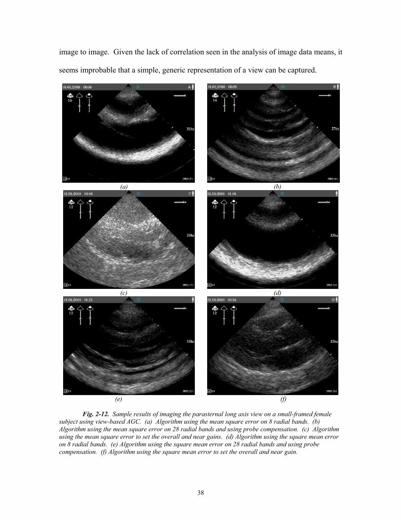
2.5.4. Results and Discussion Sample results of the six algorithms (3 gain profile applications each tested with the 2
error functions) are shown in Fig. 2-12a-f. The subject imaged was a small-framed
female. The screen shots show the first two gain profile application techniques grossly
overfit the data; there is an artificial bright band three-fourths of the way down the
image, corresponding to the spectral reflection of the parasternum seen in a typical
parasternal long axis view. Even with the second smoothing error function, the bright
artifact still occurs. The third gain profile application method works much better, since it
considers a larger number of samples in the calculation of each gain parameter.
Nevertheless, performance of this algorithm using either of the error functions was not
very consistent; it stabilized at extremely different gain settings when the experiments
were repeated.
The chief reasons for poor performance are probably the overfitting due to so many
bands, and the use of an inappropriate representation of the target data set. The relative
success of the last gain profile application method, however, underscores the fact that
achieving acceptable AGC is much likelier if only a few gain parameters are set. By
virtue of the fact that the first error function tries to match sample for sample, overfitting
is a very predictable behavior of these algorithms. The target data set used captures all
the details of a sample long axis image, instead of just the salient features that hold from
38
image to image. Given the lack of correlation seen in the analysis of image data means, it
seems improbable that a simple, generic representation of a view can be captured.
(a) (b)
(c) (d)
(e) (f)
Fig. 2-12. Sample results of imaging the parasternal long axis view on a small-framed female
subject using view-based AGC. (a) Algorithm using the mean square error on 8 radial bands. (b) Algorithm using the mean square error on 28 radial bands and using probe compensation. (c) Algorithm using the mean square error to set the overall and near gains. (d) Algorithm using the square mean error on 8 radial bands. (e) Algorithm using the square mean error on 28 radial bands and using probe compensation. (f) Algorithm using the square mean error to set the overall and near gain.

39
One reason for this difficulty is the inherent fact that each patient is a different size.
Although the maximum depth of interrogation can be adjusted to put the observed organ
at approximately the same location on the screen, the discreet depths available and the
different proportions of the heart (due to different inherited physiologies and different
health conditions) make each individual patient’s images quite different. In light of these
experiments with a view-based algorithm, an AGC algorithm that operates independently
of view seems more promising. Such a generic algorithm can also perform on non-
standard views, which are highly likely to occur given an inexperienced sonographer who
is simply trying to view the heart from any angle. The remainder of this thesis discusses
the development and performance of such a generic AGC algorithm.

40
Xk; Rhap uhk;
3. Correlating Mean and Blood/Tissue Composition 3.1. Motivation for Correlating Mean and Blood/Tissue Composition To design an algorithm that sets gain values based on the composition of the input image
requires an analysis of acoustic data to determine which parameters are useful in
determining the composition of an image. Since the AGC algorithm being designed must
be implemented in real time, only computationally simple parameters can be considered.
This chapter describes an investigation into the correlation between acoustic data means
and blood/tissue composition; the next chapter discusses a similar investigation into the
correlation between acoustic data variance and blood/tissue composition.
Theoretically, each sample in the acoustic data set for one frame could be classified as
blood or tissue, in the style of rational gain compensation. The primary problem with
such an approach is that from frame to frame, a sample in the same line and depth could
change its composition, because of the motion of the heart. Thus, gain values for a
particular sample could not be carried over from frame to frame. Hardware changes
could be made to apply the gain to the current sample being analyzed, but given the
architecture of the portable ultrasound device, such fine control is not possible through
software. Changing the gain profile for each line is a time-consuming hardware
operation and would reduce the frame rate. Thus, the goal is to control automatically the
manual time gain compensation (TGC) settings, and not operate on a line-by-line basis.
This consideration suggests that a block of acoustic data samples be considered together.
Since gains are only being set in the radial direction, the first approach would be to group

41
the data in radial bands. The composition of samples varies from line to line, so
classifying an entire radial band as blood or tissue is virtually impossible. A more viable
approach is to divide the acoustic data into r radial bands and l lateral bands, and each
block of this matrix could be classified as mostly blood or tissue, by looking at all the
acoustic samples in the block. Gains could be set to optimize the appearance of a
majority of blocks.
Useful image statistics must be found to classify and optimize blocks of the image. We
must be able to classify a block as blood or tissue, and then we must be able to define the
desired appearance of a block based on its classification. The simplest attribute to
consider, the mean of the values in a block of samples, can potentially answer both these
questions. The gains are set ultimately to bring the brightness of the image to a desired,
uniform level. The average value of a block is potentially a very good measure of its
appearance. Can we find an ideal target mean for a blood block or a tissue block?
Absolute means are not likely to be a good metric for classification, however; when
gains are mis-set, the means of each block would be expected to be significantly different
from the ideal means. One would reasonably expect, however, that the relative means
would be similar across images. For example, even if the gains are set extremely high,
blood samples should still have lower values that tissue samples, unless saturation occurs,
which is highly unlikely for moderate preset gain levels. Thus, the mean of each block
relative to the mean of the entire image may be a useful attribute to classify the block as

42
blood or tissue. These considerations motivate this analysis of the correlation between
block means and blood/tissue composition.
3.2. Data Collection The acoustic sample values can be collected from two different points in the processing
chain shown in Fig. 3-1. One choice is after dynamic range mapping, where the acoustic
sample values of 0 to 255 map to 48 to 96 dB (values above and below this range are
clipped to the minimum and maximum values). The dynamic-range-mapped (“B” mode)
values are the values input to the scan converter. Another choice is to use the pre-
dynamic-range-mapped (“A” mode) data, where the acoustic sample values of 0 to 255
map to 0 to 96 dB. Thus, the samples that show up as blood (value = 0) in the dynamic-
range-mapped-data occupy half the value range before dynamic range mapping. The
means of the samples can be calculated using the data from either of these points, and
both were considered.
AGCAlg.
“B” data121 lines of480 samples
0 - 255=>
48 - 96 dB
Signal fromtransducer
VariableGain and
Clip
A/DConv.
DynamicRange
Mapper
ScanConv.
Display
“A” data121 lines of 480 samples
0 - 255 => 0 - 96 dB
Fig. 3-1. Selected features of the ultrasound processing chain. The input data to the AGC algorithm can come from before dynamic range-mapping (“A” data) or after dynamic range-mapping (“B” data).

43
The data for this analysis came from Sets D and E (as described in Chapter 2), as well as
Set F (“fine”), where data was collected in finer precision. To collect Set F data, an
experienced sonographer performed the imaging, including setting the gain parameters.
The data collected represents the digitized acoustic samples from both just before
dynamic range mapping and just before scan conversion. Instead of recording each
sample’s value, frequency of value occurrence was recorded for several blocks of data for
Set F. The acoustic data set was split into 4 lateral bands (of 30 or 31 lines each) and 8
radial bands (of 60 samples each), resulting in 32 blocks of 3600 or 3720 samples each.
Sample values were considered in bins of 8, so that the number of samples having a value
from 0-7, 8-15, etc. was recorded for each block. Set F contains these frequency of
occurrence data for five different frames of each of the four standard views taken at
initial preset, good, low and high gain settings. The subject for Set F was a medium-
frame, easy-to-image female. Each image corresponding to the data collected in Set D, E
and F was split into 4 radial bands by 4 lateral bands (Sets D and E) or 8 radial bands by
4 lateral bands (Set F). Each of these block were hand-classified as blood or tissue.
3.3. Target Means for Blood and Tissue Composition 3.3.1. Target Dynamic-Range-Mapped Means To arrive at target means for blood and tissue blocks, the frequency of means in hand-
classified blood and tissue blocks from Set E, Set D and Set F data were examined. The
number of blocks with means that fell in ranges of size 8 (i.e. 0-7, 8-15, etc.) were
counted, and these counts were normalized over the total number of blocks. Fig. 3-2
shows the frequency of dynamic-range-mapped, “B” data means for blood and tissue
blocks for Set E, Set D and Set E and D combined (blocks from a 4 x 4 grid). The

44
histograms show that whether dealing with a difficult-to-image patient (Set D) or an
easy-to-image patient (Set E), the means for tissue and blood blocks fall in distinctly
different ranges. The histograms also demonstrate the distribution of block means for
different patients is fairly similar. The peak mean for blood blocks occurs between 24 –
32 for both Set D and Set E data. The peak mean for tissue occurs between 40 – 48 for
Set D, and between 56 – 64 for Set E, and the second highest peak for the Set D tissue
blocks also falls in the range of 56 - 64. The histograms illustrate that the range of means
for tissue is much wider for tissue than for blood. More than 5% of the tissue blocks in
both Set D and Set E data have means over 90. Looking at both sets of data together,
blood means fall in a range of width approximately 70, whereas the tissue blocks fall in a
range of width approximately 110.
0
0.05
0.1
0.15
0.2
0.25
0.3
0.35
0.4
3.5 11.5 19.5 27.5 35.5 43.5 51.5 59.5 67.5 75.5 83.5 91.5 99.5 107.5 115.5 123.5 131.5 139.5Mean
Freq
uenc
y
Blood - DBlood - E
Blood - TotalTissue - D
Tissue - ETissue - Total
Fig. 3-2. Frequency of occurrence of dynamic-range-mapped (“B” data) block means for blood and tissue blocks for data generated with good gains settings on difficult-to-image (“D”) and easy-to-image (“E”) subjects.

45
0
0.05
0.1
0.15
0.2
0.25
3.5 11.5 19.5 27.5 35.5 43.5 51.5 59.5 67.5 75.5 83.5 91.5 99.5 107.5 115.5 123.5 131.5 139.5 147.5 155.5 163.5 171.5 179.5 187.5
Mean
Freq
uenc
y
BloodTissue
Fig. 3-3. Frequency of occurrence of dynamic-range-mapped (“B” data) block means for blood and tissue blocks for data generated with good manual gains (Set F data).
0
0.05
0.1
0.15
0.2
0.25
0.3
0.35
0.4
67.5 75.5 83.5 91.5 99.5 107.5 115.5 123.5 131.5 139.5 147.5 155.5 163.5 171.5 179.5 187.5 195.5 203.5 211.5 219.5 227.5 235.5 243.5 251.5
Mean
Freq
uenc
y
BloodTissue
Fig. 3-4. Frequency of occurrence of pre-dynamic-range-mapped (“A” data) block means for blood and tissue blocks for data generated with good manual gains (Set F data).
Fig. 3-3 shows a similar plot using dynamic-range-mapped “B” data from the good
manual gain setting Set F blocks (from an 8 x 4 grid). Similar to the previous data, the

46
peak blood block mean occurs between 24 – 32, and the highest peaks for tissue blocks
occur between 40 – 48, 64 – 72 and 56 – 64. The range of tissue means, approximately
of a width of 150, is again much greater than the range of blood means, approximately of
a width of 95.
3.3.2. Target Pre-Dynamic-Range-Mapped Means
Fig. 3-4 shows an identical plot using the pre-dynamic-range-mapped “A” data from the
good manual gain setting Set F blocks. The peak blood mean, between 136 – 144, and
the peak tissue mean, between 144 – 152, are much closer in value than the dynamic-
range-mapped peak means. The range of tissue block means, approximately 85, is wider
than the range of blood block means, approximately 60, and the frequencies of
occurrence fall off more slowly as values increase than as they decrease. The range
widths for both blood block means and tissue block means are smaller than the
corresponding range widths for the dynamic-range-mapped data.
3.3.3. Conclusions from Target Mean Analysis
Both the dynamic-range-mapped data and the pre-dynamic-range-mapped data analyses
suggest that the blood block means should be around 52 – 53 dB and the tissue block
means should be around 55-59 dB. Since the separation between the blood and tissue
peak means is more pronounced in the dynamic-range-mapped data, it seems better to
define the target means in terms of the dynamic-range-mapped scale. Fig. 3-2, 3-3, and
3-4, however, all show a significant overlap between blood and tissue block means. This
overlap is probably due to the large block size. A block from 4 x 4 grid, or even an 8 x 4

47
grid, will most likely contain some samples that correspond to blood and some samples
that correspond to tissue, making the composition of the block bimodal. During manual
classification, there were several blocks encountered that were nearly half-blood and half-
tissue. A smaller block size would increase the chance of having unimodal block
composition. As block compositions become more uniform, it would be expected that
the target blood mean would lower and that the target tissue mean would rise.
Another practical consideration is to categorize tissue blocks into two more specific
classes, ordinary tissue blocks, and specular tissue blocks, that would have higher means,
due to the spread of tissue means. Blocks containing the specular reflections off the
pericardium would be an example of “tissue” blocks that have unusually high means.
Taking these observations and conjectures into account, a target blood mean (in terms of
dynamic-range-mapped values) of under 32, a target tissue mean around 64 and a target
specular mean over 90 are the suggested starting parameter values for a classification-
based AGC algorithm.
3.4. Determining Blood and Tissue Composition from Normalized Means For the successful implementation of a classification-based AGC algorithm, it is
necessary to find attributes to aid in the classification of blocks of data in addition to
defining the optimum appearance of each block. The normalized mean for each block,
that is, the mean of each block relative to the overall mean of data set, is potentially a
good attribute for classifying a block. Unless the gains cause the sample values to
saturate, which is highly unlikely at usual gain levels, areas that should be dark in an

48
image will be darker than areas that should be bright in an image, even if the whole
image is too bright or too dark.
3.4.1. Dynamic-Range-Mapped Relative Means
0
0.05
0.1
0.15
0.2
0.25
0.3
0.35
3.5 11.5 19.5 27.5 35.5 43.5 51.5 59.5 67.5 75.5 83.5 91.5 99.5 107.5 115.5 123.5 131.5 139.5 147.5 155.5 163.5 171.5 179.5 187.5
Relative Mean
Freq
uenc
y InitGoodLowHigh
(a)
0
0.02
0.04
0.06
0.08
0.1
0.12
0.14
0.16
0.18
3.5 11.5 19.5 27.5 35.5 43.5 51.5 59.5 67.5 75.5 83.5 91.5 99.5 107.5 115.5 123.5 131.5 139.5 147.5 155.5 163.5 171.5 179.5 187.5
Relative Mean
Freq
uenc
y InitGoodLowHigh
(b)
Fig. 3-5. Histograms showing the frequency of occurrence of dynamic-range-mapped (“B” data) block means for frames created with initial preset, good, low and high gain settings. (a) Tissue blocks. (b) Blood blocks. (Set F data.)

49
0
0.05
0.1
0.15
0.2
0.25
0.3
-92.5 -84.5 -76.5 -68.5 -60.5 -52.5 -44.5 -36.5 -28.5 -20.5 -12.5 -4.5 3.5 11.5 19.5 27.5 35.5 43.5 51.5 59.5 67.5 75.5 83.5 91.5
Relative Mean
Freq
uenc
y InitGoodLowHigh
(a)
0
0.05
0.1
0.15
0.2
0.25
0.3
-92.5 -84.5 -76.5 -68.5 -60.5 -52.5 -44.5 -36.5 -28.5 -20.5 -12.5 -4.5 3.5 11.5 19.5 27.5 35.5 43.5 51.5 59.5 67.5 75.5 83.5 91.5
Relative Mean
Freq
uenc
y InitGoodLowHigh
(b)
Fig. 3-6. Histograms showing the frequency of occurrence of dynamic-range-mapped (“B” data) block relative means for frames created with initial preset, good, low and high gain settings. (a) Tissue blocks. (b) Blood blocks. (Set F data.)
Fig. 3-5a and b show the frequency of absolute dynamic-range-mapped (“B”) means for
hand-classified blood and tissue blocks from images with four different gain settings: the

50
current preset (initial) manual gain settings, good manual gain settings, low manual gain
settings and high manual gain settings. These histograms clearly show that the
distribution of means is quite different for different gain settings, and there is significant
overlap in the mean ranges between different composition types. For example, the peak
tissue mean for low manual gain settings (between 40 – 48) is less that many of the
secondary peaks of the blood mean for high manual gain settings (between 80 – 120).
0
0.05
0.1
0.15
0.2
0.25
-92.5 -84.5 -76.5 -68.5 -60.5 -52.5 -44.5 -36.5 -28.5 -20.5 -12.5 -4.5 3.5 11.5 19.5 27.5 35.5 43.5 51.5 59.5 67.5 75.5 83.5 91.5
Relative Mean
Freq
uenc
y
BloodTissue
Fig. 3-7. Histograms showing the frequency of occurrence of dynamic-range-mapped (“B” data) block relative means for frames created with varying gain settings for both tissue block and blood blocks. (Set F data.)
In contrast, the histograms of dynamic-range-mapped (“B”) relative means, shown in Fig.
3-6, show that the distribution of relative means is quite similar among images produced
with different gain settings. The relative peaks for blood blocks for all the four different
gain settings fall between –48 to –26, and for tissue blocks, the relative mean peaks all
fall between –26 to 16. Fig. 3-7 shows the histograms for relative dynamic-range-mapped

51
means for all of the Set F blood and tissue blocks (all the different manual gain settings
data combined together). Although there is overlap, the blood and tissue peaks are
distinct, between –40 to –32 for blood blocks and between 0 to 8 for tissue blocks. There
is some significant overlap between the two histograms, mainly between –40 to 8 (a
width of 48). Several of the blocks, however, were nearly half-tissue and half-blood,
which could help to explain the overlap between the blood and tissue relative mean
histograms. As seen with the target mean histograms, the tissue relative mean histogram
is much more spread out than the blood relative mean histogram.
3.4.2. Pre-Dynamic-Range-Mapped Relative Means
Fig. 3-8 shows the frequency of absolute pre-dynamic-range-mapped (“A”) means for
hand-classified blood and tissue blocks from images with the four different gain settings.
These data exhibit a similar lack of histogram correlation between images with different
gain settings as the dynamic-range-mapped (“B”) histograms in Fig. 3-5.
Fig. 3-9 shows the relative pre-dynamic-range-mapped mean histograms for blood and
tissue blocks at four different gain settings. The histograms have similar shapes, even
with differing gain settings. The peak relative means all fall between –16 to 0 for blood
blocks, and between –8 to 8 for tissue blocks. Fig. 3-10 shows the histograms for relative
pre-dynamic-range-mapped means for all Set F blood and tissue blocks (all manual gain
settings). The blood peak falls between –8 – 0, and the tissue peak falls between 0 – 8.
The second tissue peak falls between –8 and 0.

52
0
0.05
0.1
0.15
0.2
0.25
0.3
0.35
0.4
3.5 11.5
19.5
27.5
35.5
43.5
51.5
59.5
67.5
75.5
83.5
91.5
99.5
107.5
115.5
123.5
131.5
139.5
147.5
155.5
163.5
171.5
179.5
187.5
195.5
203.5
211.5
219.5
227.5
235.5
Relative Mean
Freq
uenc
y InitGoodLowHigh
(a)
0
0.05
0.1
0.15
0.2
0.25
0.3
3.5 11.5
19.5
27.5
35.5
43.5
51.5
59.5
67.5
75.5
83.5
91.5
99.5
107.5
115.5
123.5
131.5
139.5
147.5
155.5
163.5
171.5
179.5
187.5
195.5
203.5
211.5
219.5
227.5
235.5
Relative Mean
Freq
uenc
y InitGoodLowHigh
(b)
Fig. 3-8. Histograms showing the frequency of occurrence of pre-dynamic-range-mapped (“A” data) block means for frames created with initial preset, good, low and high gain settings. (a) Tissue blocks. (b) Blood blocks. (Set F data.)

53
0
0.05
0.1
0.15
0.2
0.25
0.3
0.35
-92.5 -84.5 -76.5 -68.5 -60.5 -52.5 -44.5 -36.5 -28.5 -20.5 -12.5 -4.5 3.5 11.5 19.5 27.5 35.5 43.5 51.5 59.5 67.5 75.5 83.5 91.5
Relative Mean
Freq
uenc
y InitGoodLowHigh
(a)
0
0.05
0.1
0.15
0.2
0.25
0.3
-92.5 -84.5 -76.5 -68.5 -60.5 -52.5 -44.5 -36.5 -28.5 -20.5 -12.5 -4.5 3.5 11.5 19.5 27.5 35.5 43.5 51.5 59.5 67.5 75.5 83.5 91.5
Relative Mean
Freq
uenc
y InitGoodLowHigh
(b)
Fig. 3-9. Histograms showing the frequency of occurrence of pre-dynamic-range-mapped (“A” data) block relative means for frames created with initial preset, good, low and high gain settings. (a) Tissue blocks. (b) Blood blocks. (Set F data.)
The overlap between the blood and tissue pre-dynamic-range-mapped relative mean
histograms can again be partially explained by the number of blocks that were nearly

54
half-tissue and half-blood. Nevertheless, both the blood and tissue histograms are
narrower than the dynamic-range-mapped relative mean histograms. In addition, the
relative mean peak for good gain setting tissue blocks is less than both the low and high
gain setting blood blocks’ relative mean peak.
0
0.05
0.1
0.15
0.2
0.25
0.3
0.35
-92.5 -84.5 -76.5 -68.5 -60.5 -52.5 -44.5 -36.5 -28.5 -20.5 -12.5 -4.5 3.5 11.5 19.5 27.5 35.5 43.5 51.5 59.5 67.5 75.5 83.5 91.5
Relative Mean
Freq
uenc
y
BloodTissue
Fig. 3-10. Histograms showing the frequency of occurrence of pre-dynamic-range-mapped (“A” data) block relative means for frames created with varying gain settings for both tissue block and blood blocks. (Set F data.)
3.4.3. Conclusions from Relative Mean Analysis
These observations suggest that the dynamic-range-mapped data relative mean is a more
robust attribute for classification than the pre-dynamic-range-mapped data relative mean.
The overlap between the blood and tissue normalized dynamic-range-mapped mean
histograms in Fig. 3-8 emphasize the need to use smaller block sizes to reduce the
bimodality of blocks. The spreading of the tissue histogram reinforces the idea that tissue
blocks should be classified as ordinary tissue or specular tissue blocks. These histogram
data suggest that a dynamic-range-mapped relative mean under –32 is a good starting
value for the AGC algorithm parameter that classifies blocks as blood. Relative means
above 32 would be a starting value for the algorithm parameter that classifies blocks as

55
specular tissue. Blocks that fall between the two values would be classified as ordinary
tissue. The use of smaller blocks sizes, which would presumably increase the degree of
unimodality of a block’s samples, could alter these precise values; nevertheless, the
degree of separation between the blood and tissue relative mean histograms despite the
relatively large blocks sizes used in collecting the Set F data, support the use of relative
means to determine the composition of a block.

56
Xk; Rhap uhk;
4. Correlating Variance and Blood/Tissue Composition 4.1. Motivation for Correlating Variance and Blood/Tissue Composition Although mean is the simplest indicator to use for classifying a block of acoustic data as
tissue or blood, this investigation of AGC algorithms also considered another possible
indicator, variance. Fig. 4-1a and b show portions of an ultrasound image that are mostly
blood and mostly tissue, respectively. These images show that blood appears far more
uniform than tissue. Tissue is not uniform in its composition; for example, tissue also
contains blood, from the capillaries that permeate the tissue. This variability leads to a
high variance in the acoustic reflections from tissue. In the case of blood on the other
hand, the scatterers produce more uniform responses. In addition, dynamic range
mapping takes all sample values below 48 dB to 48 dB, so that low values are all mapped
to the same value. Thus, the samples coming back from tissue will cover a much broader
span of values than a set of blood samples, both due to the inherent nature of tissue and
blood, and the processing applied to the incoming signals. This observation suggests that
the variance of the samples in a block of acoustic data will be significantly higher if the
block contains mostly tissue than if it contains mostly blood.
(a) (b)
Fig. 4-1. (a) Blood and (b) tissue regions from a cardiac ultraound image.
Fig. 4-2 shows a plot of dynamic-range-mapped “B” mean vs. “B” variance of all of the
four radial bands of all the images in data sets E and D. Tissue has higher means than

57
blood, and bands with higher variances also have higher means. Nevertheless, the nearly
linear relationship seen in Fig. 4-2 suggests that the correlation between mean and
variance may only be due to noise. Noise and bimodality (the presence of both tissue and
blood in a given block of data) may also contribute to the variance of the samples in a
block. The data from Set E and D were analyzed to determine if the variance caused by
tissue composition could dominate block variance sufficiently to classify a block.
0
500
1000
1500
2000
2500
3000
3500
0 20 40 60 80 100 120
Mean
Varia
nce
plx - Dshx - Dap4 - Dsbc - Dplx - Eshx - Eap4 - Esbc - E
Fig. 4-2. Dynamic-range-mapped mean vs. variance of radial bands for different views on different subjects. The acoustic data was split into four approximately equal radial bands, and the mean and variance were calculated for each band.
4.2. Data Collection Data Sets D, E (as described in Chapter 2) and F (as described in Chapter 3), were used
for this analysis.
4.3. Determining Blood and Tissue Composition from Variance 4.3.1. Dynamic-Range-Mapped Variance Fig. 4-3 shows a histogram of the variances calculated from the dynamic-range-mapped
samples “B” in blood blocks and tissue blocks from Set D, Set E and Sets D and E

58
combined. Variances were grouped in bins of size 250. This plot shows that even for
images with good gain settings, the variance distributions for blood and tissue are
different but have significant overlap. This overlap may be due to the large block size
used in collecting the Set D and E data. A larger block size results in more blood blocks
that contain some tissue, and tissue blocks that contain some blood. Thus, the variance
may be strongly influenced by its bimodality component more than the composition
component.
0
0.05
0.1
0.15
0.2
0.25
0.3
125 375 625 875 1125 1375 1625 1875 2125 2375 2625 2875 3125 3375 3625 3875 4125 4375 4625 4875
Relative Mean
Freq
ency
Blood - EBlood - D
Blood - TotalTissue - ETissue - D
Tissue - Total
Fig. 4-3. Histogram of the dynamic-range-mapped “B” variances in blood and tissue blocks of acoustic data from imaging both easy (E) and difficult (D) to image patients.
Data set F was collected using a finer block size (8 radial bands by 4 lateral bands), and it
also provides block statistics for cases where the gains are poorly set. Fig. 4-4a and b
show histograms of variances of the dynamic-range-mapped “B” sample values of blood
and tissue blocks from images at initial preset, good, low and high gain settings. The plot
shows that the variance distributions vary greatly for different gain settings; the peak
variances for blood blocks span a range of over 1250, and the peak variances for tissue

59
blocks span a range of over 750. The variance distributions for tissue blocks are more
similar among different gain settings than the variance distributions for blood.
0
0.05
0.1
0.15
0.2
0.25
0.3
124.5 374.5 624.5 874.5 1125 1375 1625 1875 2125 2375 2625 2875 3125 3375 3625 3875 4125 4375 4625 4875
Variance
Freq
uenc
y
In itG oodLowHigh
(a)
0
0.05
0.1
0.15
0.2
0.25
0.3
124.5 374.5 624.5 874.5 1125 1375 1625 1875 2125 2375 2625 2875 3125 3375 3625 3875 4125 4375 4625 4875
Variance
Freq
uenc
y
In itG oodLowHigh
(b)
Fig. 4-4. Histograms of the dynamic-range-mapped “B” variances in (a) blood and (b) tissue blocks of acoustic data from ultrasound images generated with preset, good, low and high gain settings. (Set F data.)

60
This phenomenon can perhaps be partially explained by the fact low gain settings may
push many weak signal values below the lower limit of the dynamic range, so that they
all map to 48 dB, thereby reducing the variance. Alternatively, high gain settings may
push some weak signal values above the lower threshold, pushing them into the typical
tissue range, thereby increasing the variance of a set of samples in a blood block. For
tissue blocks, this non-linear effect is not likely to happen; gains are rarely so high that
the signal is saturated. Fig. 4-5 shows a histogram for the variance of all blood and tissue
blocks from Set F. Although the distributions vary between the two composition types,
the histograms are not very separable; there is no cutoff variance value below which
most blocks are blood, and above which most blocks are tissue.
0
0.02
0.04
0.06
0.08
0.1
0.12
0.14
0.16
0.18
0.2
124.5 374.5 624.5 874.5 1125 1375 1625 1875 2125 2375 2625 2875 3125 3375 3625 3875 4125 4375 4625 4875
Variance
Freq
uenc
y
BloodTissue
Fig. 4-5. Histograms of the dynamic-range-mapped “B” variances in blood and tissue blocks of acoustic data from ultrasound images generated with varying gain settings (preset, good, low and high gain settings). (Set F data.)

61
4.3.2. Pre-Dynamic-Range-Mapped Variance
Fig. 4-6a and b show variance histograms for pre-dynamic-range-mapped “A” sample
values for blood and tissue blocks from images produced with different gain settings. For
pre-dynamic-range-mapped data, the histograms between different gain settings are far
more similar among images with different gain settings.
0
0.1
0.2
0.3
0.4
0.5
0.6
0.7
124.5 374.5 624.5 874.5 1125 1375 1625 1875 2125 2375 2625 2875 3125 3375 3625 3875 4125 4375 4625 4875
Variance
Freq
uenc
y
In itGoodLowH igh
(a)
0
0.1
0.2
0.3
0.4
0.5
0.6
124.5 374.5 624.5 874.5 1125 1375 1625 1875 2125 2375 2625 2875 3125 3375 3625 3875 4125 4375 4625 4875
Variance
Freq
uenc
y
In itG oodLowHigh
(b)
Fig. 4-6. Histograms of the pre-dynamic-range-mapped “A” variances in (a) blood and (b) tissue blocks of acoustic data from ultrasound images generated with preset, good, low and high gain settings. (Set F data.)
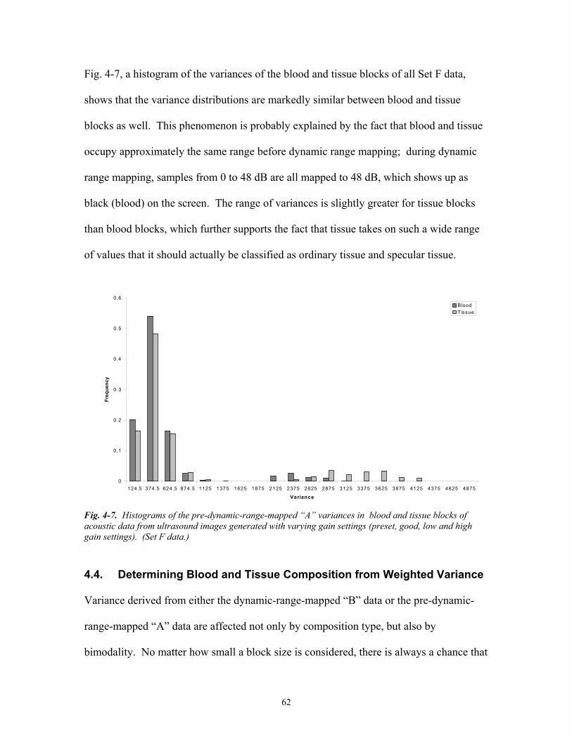
62
Fig. 4-7, a histogram of the variances of the blood and tissue blocks of all Set F data,
shows that the variance distributions are markedly similar between blood and tissue
blocks as well. This phenomenon is probably explained by the fact that blood and tissue
occupy approximately the same range before dynamic range mapping; during dynamic
range mapping, samples from 0 to 48 dB are all mapped to 48 dB, which shows up as
black (blood) on the screen. The range of variances is slightly greater for tissue blocks
than blood blocks, which further supports the fact that tissue takes on such a wide range
of values that it should actually be classified as ordinary tissue and specular tissue.
0
0.1
0.2
0.3
0.4
0.5
0.6
124.5 374.5 624.5 874.5 1125 1375 1625 1875 2125 2375 2625 2875 3125 3375 3625 3875 4125 4375 4625 4875
Variance
Freq
uenc
y
BloodTissue
Fig. 4-7. Histograms of the pre-dynamic-range-mapped “A” variances in blood and tissue blocks of acoustic data from ultrasound images generated with varying gain settings (preset, good, low and high gain settings). (Set F data.)
4.4. Determining Blood and Tissue Composition from Weighted Variance Variance derived from either the dynamic-range-mapped “B” data or the pre-dynamic-
range-mapped “A” data are affected not only by composition type, but also by
bimodality. No matter how small a block size is considered, there is always a chance that

63
a few samples of the opposite composition type will be contained in the block, which will
increase the variance of the samples in the block. In an attempt to filter out the variance
due to bimodality, a “weighted variance” was calculated using the pre-dynamic-range-
mapped “A” data. This calculation first makes the assumption that samples with values
below 48 dB (0 through 127 on the pre-dynamic-range-mapped values scale) are
primarily blood (since they appear black on the screen) and samples with values above 48
dB (128 through 255 on the scale) are primarily tissue. The samples in a block are split
into those whose pre-dynamic-range-mapped values fall below 128, and those whose
values are 128 and above. The variance for the lower-valued samples is calculated, as
well as the variance for the higher-valued samples, after mapping them from 128-255 to
0-127, so that they are on the same scale as the lower-valued variances. These variances
are then averaged together, weighted by the number of samples used to derive each
variance. Thus,
NNN 2
HH2LL2
Wσ+σ
=σ
where σW2 is the weighted variance, NL is the number of low-valued samples, NH is the
number of high-valued samples, σL2 is variance of low-valued samples, σH
2 is the scaled
variance of high-valued samples and NL + NH = N is the total number of samples.
Fig. 4-8a and b show the weighted variance histograms for blood and tissue blocks from
Set F images generated with different gain settings. The variance distributions vary
greatly for different gain settings.

64
0
0 .1
0 .2
0 .3
0 .4
0 .5
0 .6
0 .7
1 2 4 . 5 3 7 4 .5 6 2 4 .5 8 7 4 .5 1 1 2 5 1 3 7 5 1 6 2 5 1 8 7 5 2 1 2 5 2 3 7 5 2 6 2 5 2 8 7 5 3 1 2 5 3 3 7 5 3 6 2 5 3 8 7 5 4 1 2 5 4 3 7 5 4 6 2 5 4 8 7 5
V a r ia n c e
Freq
uenc
y
In itG o o dL o wH ig h
(a)
0
0 . 1
0 . 2
0 . 3
0 . 4
0 . 5
0 . 6
1 2 4 .5 3 7 4 .5 6 2 4 .5 8 7 4 .5 1 1 2 5 1 3 7 5 1 6 2 5 1 8 7 5 2 1 2 5 2 3 7 5 2 6 2 5 2 8 7 5 3 1 2 5 3 3 7 5 3 6 2 5 3 8 7 5 4 1 2 5 4 3 7 5 4 6 2 5 4 8 7 5
V a r ia n c e
Freq
uenc
y
I n itG o o dL o wH ig h
(b)
Fig. 4-8. Histograms of the weighted variances in (a) blood and (b) tissue blocks of acoustic data from ultrasound images generated with preset, good, low and high gain settings. (Set F data.)
This observation is perhaps explained by an examination of an ultrasound image
generated at high gain settings, shown in Fig. 4-9a. In this image, the chambers of the
heart, although darker than the surrounding tissue, are filled with bright, visible clutter.
This clutter negates the initial assumption that blood takes on values below 48 dB; in
actuality, if gain settings are too high, blood samples may take on values above the
threshold. As seen in Fig. 4-9b, which is a cardiac ultrasound image generated at low

65
gain settings, the blood chambers are “too clean”, so that the clutter around the
endocardial borders and the valves come close to disappearing. This result certainly
means that most blood sample values fall below 48 dB, and Fig. 4-8a indicates that
weighted variances at low gain settings rarely take on values above 300. For a good
image, however, there will be some clutter in blood and the valves will be visible, so that
there will be some small but not insignificant contribution from the high-value variance.
Thus, the weighted variance distributions vary significantly among blocks from images
with different gain settings.
(a) (b)
Fig. 4-9. Cardiac ultrasound images generated with poor gain settings. (a) Apical four chamber view generated with high gain settings. Note that the chamber is filled with bright clutter, making it appear similar to tissue. (b) Parasternal long axis view generated with low gain settings. Note how the valves are not sharply delineated. The assumption that all blood samples fall below 48 dB is not a good one. The overlap
between the high gain setting variance distribution for blood and the other gain settings’
distributions for tissue suggest that once blood signals have been amplified to fall in the
tissue value range, the statistics of the samples do not greatly differ. Even if the
assumption is true in some cases and variance due to bimodality has somewhat been
filtered out, for a block that has a significant number of high-valued and low-valued

66
samples, neither the low value nor the high value variance’s contribution to the weighted
variance is negligible. Thus, without smaller block sizes, the range of weighted variances
for a given composition type will still span a significant range.
4.5. The Use of Variance to Classify Blocks as Blood or Tissue The results from these analyses of the data from Sets D, E and F suggest that variance is
not a good indicator of tissue composition. A block almost always contains some
samples from the non-dominant composition type that causes the simple variance of the
block’s dynamic-range-mapped samples to increase due the bimodality of the sample
types. This effect is only increased when considering pre-dynamic-range-mapped “A”
samples, since these samples have not been processed through the non-linear clipping
that maps all low values to 48 dB, thereby reducing the variance of dark blood blocks.
The weighted variance that attempts to lessen the contribution of bimodality to the
variance faces the same problem that we are attempting to address: how to distinguish
blood samples from tissue samples; a static cutoff among all images is not adequate.
The initial and logical hypothesis that the variance of the samples in a blood block would
be less than the variance of the samples in a tissue block is supported inasmuch that the
blood blocks’ variance distributions are always heavier in the lower values than the tissue
blocks’ variance distributions. This distinction, however, is not so significant as to be the
basis of a classification scheme.

67
Xk; Rhap uhk;
5. Classification-Based AGC Algorithms 5.1. Overview of the Classification-Based AGC Algorithms The class-based AGC algorithm, summarized in Fig. 5-1, is encoded in a routine
agc_calc() that is called each time an entire frame of acoustic data has been acquired.
The pre-scan-converted, dynamic-range-mapped “B” data samples are used to determine
appropriate overall and near gain settings for the following frame, which, like manually
set values, are applied partially before A/D conversion, and partially after. The set of
classification-based AGC algorithms considered here have two components,
classification and control. The classification component uses the input acoustic data to
classify non-overlapping blocks of data as blood, ordinary tissue (“tissue”) or specular
tissue (“specular”). The control component uses the information about the composition
of the view to determine what the gains ought to be. There are several parameters that
control the behavior of the algorithm; these are described in the text of this chapter, and
summarized in Fig. 5-2.
Timing:– Frame f0: Classify
Choose to increment/decrement overall gain– Frames f1 - fn: Adjust overall gain– Frame fn+1: Choose to increment/decrement near gain– Frames fn+2 - fn+1+m: Adjust near gain
......f1 fnf0 fn+1 fn+1+mfn+2
Fig. 5-1. An overview of the classification-based AGC algorithm and its timing.
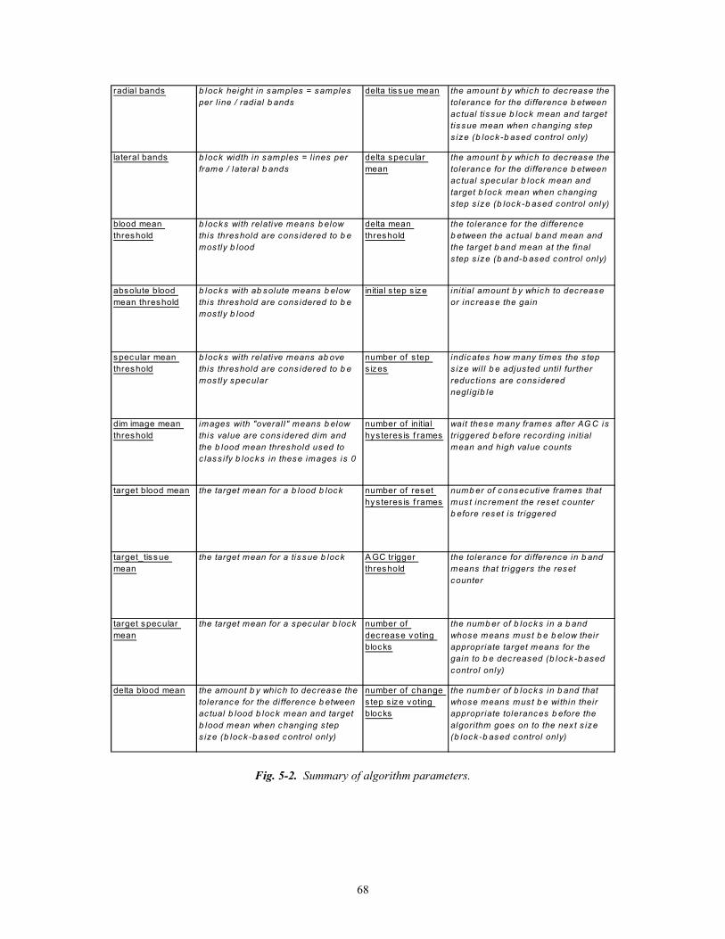
68
radial bands b lock height in samples = samples per l ine / radial b ands
delta tissue mean the amount b y which to dec rease the tolerance for the difference b etween ac tual tissue b lock mean and target tissue mean when changing s tep s ize (b lock -b ased control only)
lateral bands b lock width in samples = l ines per frame / lateral b ands
delta specular mean
the amount b y which to dec rease the tolerance for the difference b etween ac tual specular b lock mean and target b lock mean when changing s tep s ize (b lock -b ased control only)
blood mean threshold
b locks with relative means b elow this threshold are cons idered to b e mos tly b lood
delta mean threshold
the tolerance for the difference b etween the ac tual b and mean and the target b and mean at the final s tep s ize (b and-b ased control only)
absolute blood mean threshold
b locks with ab solute means b elow this threshold are cons idered to b e mos tly b lood
initial s tep s ize initial amount b y which to dec rease or inc rease the gain
specular mean threshold
b locks with relative means ab ove this threshold are cons idered to b e mos tly specular
number of s tep s izes
indicates how many times the s tep s ize wil l b e adjus ted unti l further reduc tions are cons idered negl igib le
dim image mean threshold
images with "overal l" means b elow this value are cons idered dim and the b lood mean threshold used to c lass i fy b locks in these images is 0
number of initial hys teres is f rames
wait these many frames after AG C is tr iggered b efore recording initial mean and high value counts
target blood mean the target mean for a b lood b lock number of reset hys teres is f rames
numb er of consecutive frames that mus t inc rement the reset counter b efore reset is tr iggered
target_tissue mean
the target mean for a tissue b lock A GC trigger threshold
the tolerance for difference in b and means that tr iggers the reset counter
target specular mean
the target mean for a specular b lock number of dec rease voting blocks
the numb er of b locks in a b and whose means mus t b e b elow their appropriate target means for the gain to b e dec reased (b lock -b ased control only)
delta blood mean the amount b y which to dec rease the tolerance for the di fference b etween ac tual b lood b lock mean and target b lood mean when changing s tep s ize (b lock -b ased control only)
number of change s tep s ize voting blocks
the numb er of b locks in b and that whose means mus t b e within their appropriate tolerances b efore the algorithm goes on to the nex t s ize (b lock -b ased control only)
Fig. 5-2. Summary of algorithm parameters.

69
The AGC process commences when an AGC reset is triggered. At this point, the
algorithm sets the overall and near gains back to their default values. INIT_
HYSTERESIS_FRAMES is the parameter that defines the delay (in frames) before a
frame’s acoustic data samples are used to initialize the composition classifications for the
view. The gains are reset to default values so that classification always occurs under the
same conditions. This delay is implemented to make sure the transducer is in a steady
position before classification occurs.
Step 1: Increment/decrement decision
Step 2: Adjust gain
Is tolerance criteria met?
T F
STOP
n < NUM_STEPS_SIZES
T F
Go to next step size(n++)
Adjust gain by 100/n
Does gain exceed MIN/MAX limits?
T F
NUM_STEP_SIZES = 5 MIN/MAX limits = -800/800
Fig. 5-3. Summary of gain adjustment control of algorithm.
The classification output is used to control the gain settings, first the overall gain, then
the near gain, as shown in Fig. 5-3. INIT_STEP_SIZE determines the initial increment
or decrement by which the given gain setting is adjusted. When the criteria for changing
step size is reached, the amount by which the gain is adjusted is reduced; on the nth step
size, the gain is adjusted by INIT_STEP_SIZE / n. Thus, the gain is adjusted in finer and
finer increments. NUM_STEP_ SIZES sets the total number of step sizes. All
implementations of the algorithm use NUM_STEP_SIZES = 5.

70
We define the far band as the lower 3/8ths of the image, and the near band as the next
3/8ths of the image. The top fourth of the image is excluded since it is nearly always
noise. The data from the far band first determine whether the overall gain should be
increased or decreased. After the stopping criteria has been reached on the last step size
for the overall gain, the algorithm uses the current means and the pre-determined
classifications of near band, to decide whether the near gain should be incremented or
decremented. The near gain is then adjusted on each frame just as the overall gain was.
The method of determining whether to increase or decrease the gain settings, when to
change the step size and when to stop gain adjustments vary among different
implementations.
For each frame, calculate the near and far band means, mn and mf.For either band b, does
|mb - previous_overall_meanb| > AGC_TRIGGER_THRESHOLD ?
T F
Increment reset_trigger_counter
reset_trigger_counter >RESET_HYSTERESIS_FRAMES
•previous_overall_meann = mn •previous_overall_meanf = mf•reset_trigger_counter = 0
F
T F
•set gains to default values (overall gain = -100, near gain = 0)•wait for INIT_HYSTERESIS_FRAMES,then start classification
Fig. 5-4. An illustration of the reset trigger mechanism in the AGC algorithm.

71
The reset trigger mechanism, illustrated in Fig. 5-4, is similar for the different
implementations. For each input frame, the near band and far band means are computed.
AGC_TRIGGER_ THRESHOLD is the absolute difference in a given band’s mean
above which a reset counter is triggered. RESET_HYSTERESIS_FRAMES is the
number of frames in a row whose band means must differ from the band means of the
frame previous to the first frame that triggered the reset counter. These parameters
control the activation of the automatic gain control mechanism.
If either of the band means have not changed from the previous mean values by more that
AGC_TRIGGER_THRESHOLD, the current values are stored as the previous mean
values. Otherwise, a reset counter is triggered. The subsequent frames are compared to
the previous band mean values at the time when the counter was triggered. If
RESET_HYSTERESIS_ FRAMES frames have band means that differ from these
previous band mean values by more than AGC_TRIGGER_THRESHOLD, an AGC reset
is triggered; that is, the gains are reset to the default values and after INIT_
HYSTERESIS_FRAMES number of frames, the image composition is classified. If the
band means do not differ enough from the previous band means before the required
number of frames is reached, the counter is reset. This system of reset is designed to
filter out cases where one frame is unusually noisy or if contact becomes poor for just a
few frames. Such occurrences should not trigger a change in gain values.
In some implementations of the algorithm, a reset counter trigger can occur while the
gain adjustments are occurring; in other implementations, the reset counter is blocked

72
while adjustments are occurring. If a reset counter trigger does occur while the gains
adjustment are occurring, the gain adjustments are stopped. The benefit of resetting the
gains while adjustments are occurring is that if the transducer is moved significantly
before the final gains have been reached, the system can re-evaluate what the appropriate
gains should be. On the other hand, if a gain change causes a significant change to the
means, a reset could be triggered without a transducer shift; this possibility is avoided if
the reset is turned off while gains are being adjusted. Algorithm testing would reveal
which tradeoff performs better, although this variation was not explicitly tested in this
investigation. In addition to monitoring for transducer shifts, the algorithm also triggers a
reset to default gains and initialization whenever the user changes the focal depth.
5.2. Classification The classification component of the AGC algorithm is based on the mean and relative
mean data analyses discussed in Chapter 3. The classification algorithm is summarized
in Fig. 5-5. NUM_RADIAL_BANDS defines the granularity at which the acoustic data
is considered in the radial direction, while NUM_LATERAL_BANDS, defines the
granularity at which the acoustic data is considered in the lateral direction. The acoustic
samples data set is divided into NUM_RADIAL_BANDS by NUM_LATERAL_BANDS
non-overlapping blocks. An “overall” mean for each frame that is to be classified is
calculated as the mean of the bottom three-fourths of the image; as mentioned before, the
top fourth of the image is ignored because it is generally mostly noise. The mean for
each block is also calculated.

73
m < ABSOLUTE_BLOOD_MEAN_THRESHOLD
Blood
T F
o < DIM_IMAGE_MEAN_THRESHOLD
T F
m - o < 0
T F
Blood
m - o < BLOOD_MEAN_THRESHOLD
F T
Bloodm - o > SPECULAR_MEAN_THRESHOLD
T F
Specular Tissue
Fig. 5-5. A flow chart for the classification of one block, where m is the block mean, and o is the “overall” mean of the image.
ABSOLUTE_BLOOD_MEAN_THRESHOLD defines an absolute block mean value
below which a block is classified as blood. DIM_IMAGE_MEAN_THRESHOLD
defines an “overall” mean value, below which an image is considered extremely dim and
hence is classified slightly differently that most images. If the “overall” mean of the
image is less than DIM_IMAGE_ MEAN_THRESHOLD, any block whose mean falls
below the “overall” mean is classified as blood. These cases are there to handle input
data from either very dim images or images that consist mostly of the blood-filled
chamber, where a blood block’s mean may be so close to the “overall” mean that its
relative mean could be close to that of tissue. In all other cases, BLOOD_MEAN_
THRESHOLD and SPECULAR_MEAN_THRESHOLD define the block mean relative
to the “overall” mean at which, in most cases, blocks are considered blood and specular

74
respectively. A block whose mean falls more than BLOOD_MEAN_THRESHOLD
below the “overall” mean is classified as blood, and blocks whose “overall” mean is
SPECULAR_MEAN_THRESHOLD above the “overall” mean are classified as specular.
All other blocks are classified as tissue. This technique of classification is used in all
implementations of the AGC algorithm.
5.3. Control: Block-based Approach Two different methods of controlling the gain adjustments have been implemented. The
block-based approach, summarized in Fig. 5-6, considers the data in blocks at every step
of the way. There are several parameters that affect the behavior of the block-based
control component. TARGET_BLOOD_MEAN, TARGET_TISSUE_MEAN and
TARGET_SPECULAR_MEAN specify the ideal mean for a blood block, tissue block
and specular block respectively. These target mean values were initially set based on the
mean analyses discussed in Chapter 3, and then revised empirically. After classification,
the block-based algorithm compares the mean of each of the blocks in the far band (if
adjusting overall gain) or the blocks in the near band (if adjusting near gain), and counts
how many blocks have means below the target mean for their composition type.
NUM_DECREASE_VOTING_BLOCKS describes how many blocks in a band must
have means below their target mean for the gain to be decreased; if this number is not
reached, the gains are increased. For all implementations, NUM_DECREASE_
VOTING_BLOCKS was set to equal half the number of blocks in a band.

75
Step 1: Increment/decrement decisionIf each block has block mean mb and classification CLASSb
Is mb > TARGET_CLASSb_MEANfor over half the blocks in the band of interest?
T F
Decrement Increment
Step 2: Gain adjustment
Does the tolerance condition holdfor over 1/b the blocksin the band of interest?
T F
STOP
n < NUM_STEPS_SIZES
T F
Go to next step size(n++)
Adjust gainby 100/n
Does gain exceedMIN/MAX limits?
T F
for n = 1 through 4, b = 2;for n = 5, b = 8
Tolerance Condition:
n = 1 through n = 4tol = (NUM_STEP_SIZES - n - 1) * DELTA_CLASSb_MEANIncreasing: mb > TARGET_CLASSb_MEAN - tolDecreasing: mb <TARGET_CLASSb_MEAN + tol
n = 5Initially Increasing: mb < TARGET_CLASSb_MEANInitially Decreasing: mb >TARGET_CLASSb_MEAN
T T + ∆ T + 2∆T + 3∆T - 3∆T - 2∆ T - ∆
Fig. 5-6. Summary of block-based control for the AGC algorithm.
On each iteration of adjusting the gain settings, the means of each block in the band are
re-calculated and compared to the appropriate target mean. Given the step size, some
tolerance is set for the difference between the block mean and the target mean; this
tolerance differs for each composition type. If gains are being increased, a block mean is
checked to be above the tolerance subtracted from the target mean; if the gains are being
decreased, the block mean is checked to fall below the sum of the target mean and the
tolerance. DELTA_BLOOD_MEAN, DELTA_TISSUE_MEAN, DELTA_
SPECULAR_MEAN describe by how much the tolerance for the difference between the
current block mean and the target block mean is reduced for each change in step size.

76
For all but the last step size, at the nth step size, the tolerance for some composition type
block is set as:
(NUM_STEP_SIZES – n – 1) * DELTA_COMPOSITION_TYPE_MEAN.
NUM_CHANGE_STEP_SIZE_VOTING_BLOCKS is the parameter that specifies how
many blocks’ means must fall within the tolerance level to change the step size. For all
implementations, this parameter was set to equal a fourth of the blocks in a band.
From the formula above, it can be seen that at the penultimate step size, 4, the tolerance
for all tissue types reduced to 0. The tolerance is also 0 for the fifth, and smallest, step
size. At this step size, however, the gain adjustments are made in reverse; for example,
if the gain was incremented for step sizes 1 through 4, the gains are decremented, for step
size 5. For the adjustments to be stopped, NUM_CHANGE_STEP_SIZE_VOTING_
BLOCKS / 2 of the blocks in a band must fall above the target mean if the gain is being
increased in the last step size, or below the target mean if the gain is being decreased.
This switch in the direction of gain adjustment is simply to compensate for a possible
overshoot in gain correction, by ascertaining that not all the blocks have means to the
same one side of their target means. Fig. 5-8 shows a graph of gain over time to
demonstrate the path towards the ideal gain taken by an AGC algorithm with a block-
based control component.
5.4. Control: Band-based Approach The second control component approach, summarized in Fig. 5-7, uses the classification
data to estimate the degree of mixed composition in the near band and far band. This

77
band-based approach averages the target means of all the blocks in the near or far band to
calculate a target mean for the band. If the band mean falls below the target band mean,
the gain is increased, otherwise it is decreased. On each gain adjustment iteration, the
relevant band mean is calculated and compared to the band’s target mean.
Step 1: Increment/decrement decision target_band_mean: the average of the target means
for each block in the band of interestFor band mean b,
b > target_band_mean?
T F
Decrement Increment
Step 2: Gain adjustment
Is tolerance criteria met?
T F
STOP
n < NUM_STEPS_SIZES
T FGo to next step size
(n++)Adjust gain
by 100/n
Does gain exceedMIN/MAX limits?
T F
Tolerance Condition:
tol = (NUM_STEP_SIZES - n + 1) * DELTA_MEAN_THRESHOLD
Increasing: b > target_band_mean - tolDecreasing: b < target_band_mean + tol
TT - 3∆ T - 2∆ T - ∆T - 4∆T - 5∆ T + 3∆ T + 4∆ T + 5∆T + 2∆T + ∆
Fig. 5-7. Summary of band-based control for the AGC algorithm.
DELTA_MEAN_THRESHOLD describes by how much the tolerance for the difference
between the current band mean and the target band mean is reduced for each change in
step size. At the nth step size, the tolerance is equal to (NUM_STEP_SIZES – n + 1) *
DELTA_MEAN_THRESHOLD. Thus, DELTA_MEAN_THRESHOLD is also the
tolerance level at the smallest step size. If the gain is being increased, a band’s mean
must fall above the tolerance subtracted from its target mean for the step size to change or

78
the adjustments to stop. If the gain is being decreased, the criterion becomes that the
band’s mean must fall below the sum of the target mean and the tolerance. No switch in
the direction of gain adjustment is made at the last step size. Fig. 5-8 shows how a gain
setting progresses to the right value over time if using an AGC algorithm with a band-
based control component.
-150
-100
-50
0
50
100
150
200
250
300
1 2 3 4 5 6 7 8 9Frame number
Gai
n
Block-Based ControlBand-Based Control
Fig. 5-8. An example of how a gain setting converges to a proper value using block-based and band-based control.

79
Xkl rhap uhk;
6. Characterization of Classification-Based AGC Algorithms 6.1. Parameter Selection for Block Classification The classification component of the algorithm was first analyzed separately from the rest
of the AGC algorithm. The parameters DIM_IMAGE_MEAN_THRESHOLD,
BLOOD_MEAN_THRESHOLD and SPECULAR_MEAN_THRESHOLD were altered
to improve classification performance. Performance was assessed by testing the
algorithm on frames of data from imaging the parasternal long axis view on a small-
frame female subject with preset gains, low gains (simulating the case where the preset
gains are too low) and high gains (simulating the case where preset gains are too high).
The algorithm classifications were compared to the visual image. A block’s
classification of blood was considered appropriate if there was virtually no signal in most
of the block, (i.e. poor transducer contact), or if the block could be identified as
positioned in a cardiac chamber by a trained human. A block classification of specular
was considered appropriate if approximately a fourth of the pixels in the block were
nearly white. Other, mostly mid-level gray blocks, even with some near-black or near-
white pixels, are considered tissue. Since the AGC algorithm looks at the
appropriateness of gains over all of the blocks, it is not necessary that each block be
classified properly; as long as a majority are correctly classifed, results should be
acceptable. Classification was tested for blocks generated by a grid of 8 radial bands by
8 lateral bands, as well as 16 radial bands by 16 lateral bands. The top fourth (first 2 or
four radial bands) of the image was ignored, since these data are irrelevant to the
algorithm.

80
The initial classification parameters were DIM_IMAGE_THRESHOLD = 40,
BLOOD_MEAN_THRESHOLD = 32, SPECULAR_MEAN_THRESHOLD = 32, and
ABSOLUTE_BLOOD_MEAN_THRESHOLD = 16, as suggested by the analysis
discussed in Chapter 3. The results of these parameter selections showed that blood
blocks were underclassed, for both block sizes, especially when the gains were too high
(see Fig. 6-1.) Too many tissue blocks were incorrectly classified as specular for all the
gain settings, for both block sizes. These results suggested reducing the BLOOD_
MEAN_THRESHOLD and increasing the SPECULAR_MEAN_THRESHOLD.
The next parameter set to be tested used a BLOOD_MEAN_THRESHOLD of 25 and a
SPECULAR_MEAN_THRESHOLD of 64. In this case, a few tissue blocks were still
classified as blood but only at high gain settings. The specular classifications were
mostly acceptable (see Fig. 6-2). The next parameter set was tested with a still lower
BLOOD_MEAN_THRESHOLD, 20, and a still higher TISSUE_MEAN_THRESHOLD,
80. Noticing that the mean of the image generated with the preset image during testing of
the second parameter set, 46, was fairly close to the dim image mean threshold value of
40, the DIM_IMAGE_MEAN_THRESHOLD was reduced to 30 also. The specular
blocks were now significantly underclassified in images generated with low gain settings,
using both block sizes (see Fig. 6-3).
The next parameter set was nearly identical, except for reducing the SPECULAR_
MEAN_THRESHOLD to 70. It performed reasonably well, although a few tissue blocks
were classified as blood at high gains for the smaller-sized blocks (see Fig. 6-4). The
same parameter set with SPECULAR_MEAN_THRESHOLD reduced to 60 was also

81
tested, and also performed quite well on the larger block sizes, but again overclassified a
few blocks as blood for the smaller-sized blocks (see Fig. 6-5) . Thus, a final parameter
set using a SPECULAR_MEAN_THRESHOLD of 70 and a BLOOD_MEAN_
THRESHOLD of 25 was also tested, which classified some tissue blocks as blood for the
larger block sizes at high gains, but did well with the smaller block size (see Fig. 6-6).
These last three classification parameter sets were the basis for the classification
parameter values used in the characterization experiments described in the next section.
(a) (b) (c)
Fig. 6-1. Images used to test the first set of classification parameters (DIM_IMAGE_THRESHOLD = 40, BLOOD_MEAN_THRESHOLD = 32, SPECULAR_MEAN_THRESHOLD = 32, ABSOLUTE_BLOOD_ MEAN_THRESHOLD = 16), generated using (a) good, (b) low and (c) high gain settings. The lower right-hand corner of all three sectors had blocks that were misclassified as specular for both large and small block sizes. Some of the blood blocks at the boundary of the chambers were misclassified as tissue blocks for both block sizes in image (c).
(a) (b) (c)
Fig. 6-2. Images used to test the second set of classification parameters (DIM_IMAGE_THRESHOLD = 40, BLOOD_MEAN_THRESHOLD = 25, SPECULAR_MEAN_THRESHOLD = 64, ABSOLUTE_BLOOD_ MEAN_THRESHOLD = 16), generated using (a) good, (b) low and (c) high gain settings. Some of the blood blocks at the boundary of the chambers were misclassified as tissue blocks for both block sizes in image (c).

82
(a) (b) (c)
Fig. 6-3. Images used to test the third set of classification parameters (DIM_IMAGE_THRESHOLD = 30, BLOOD_MEAN_THRESHOLD = 20, SPECULAR_MEAN_THRESHOLD = 80, ABSOLUTE_BLOOD_ MEAN_THRESHOLD = 16), generated using (a) good, (b) low and (c) high gain settings. Some of the specular blocks between 8 and 12 cm were misclassified as tissue blocks for both block sizes in image (b).
(a) (b) (c)
Fig. 6-4. Images used to test the fourth set of classification parameters (DIM_IMAGE_THRESHOLD = 30, BLOOD_MEAN_THRESHOLD = 20, SPECULAR_MEAN_THRESHOLD = 70, ABSOLUTE_BLOOD_ MEAN_THRESHOLD = 16), generated using (a) good, (b) low and (c) high gain settings. Some of the blocks containing valves that should have been classified as tissue were classified as blood for the small block size in image (c).
(a) (b) (c)
Fig. 6-5. Images used to test the fifth set of classification parameters (DIM_IMAGE_THRESHOLD = 30, BLOOD_MEAN_THRESHOLD = 25, SPECULAR_MEAN_THRESHOLD = 70, ABSOLUTE_BLOOD_ MEAN_THRESHOLD = 16), generated using (a) good, (b) low and (c) high gain settings. Some of the tissue blocks in the on the left-hand side of the last centimeter of image (c) were misclassified as blood.

83
(a) (b) (c)
Fig. 6-6. Images used to test the sixth set of classification parameters, generated using (a) good, (b) low and (c) high gain settings. Some of the blood blocks and specular blocks were misclassified as tissue blocks in image(c) when using large block size. 6.2. Characterization of AGC Algorithms A few implementations of the classification-based AGC algorithm were selected for
clinical evaluations; that is, for testing in a simulated real-time imaging scenario with
real sonographers and subjects. These four were selected based on some characterization
experiments that evaluated different implementations’ behavior in four areas: their
ability to track the movement of the transducer on and off the body, the response time to
reach reasonable gain settings and the stability of the algorithm once it reached these
settings, the consistency of an algorithm to reach similar gain settings and the general
appearance of the images produced by the algorithm. Three different flavors of the
algorithm were characterized by imaging the parasternal long axis view on a small-
framed female; the first was a standard block-based control AGC algorithm, the second a
block-based control AGC algorithm that only used the blocks in the “sweet spot” center
half of the radial bands (i.e., the first fourth and last fourth of the lateral bands were
ignored), and the third was a standard band-based control AGC algorithm. Each of these
three were tested using an 8 radial band by 8 lateral band granularity as well as a 16
radial band by 16 lateral band granularity. The block-based control algorithms could
reset while adjusting gains; the band-based control algorithms were implemented to

84
block reset during gain adjustment. Parameter values for these algorithms are
summarized in Fig. 6-7.
Parameter Std. Block-BasedSS Block-Based Std. Band-BasedNUM_RADIAL_BANDS 8 16 8 16 8 16NUM_LATERAL_BANDS 8 16 8 16 8 16BLOOD_MEAN_THRESHOLD 20 30 20 30 20 25ABSOLUTE_BLOOD_MEAN_THRESHOLD 16 16 16 16 16 16SPECULAR_MEAN_THRESHOLD 60 60 60 60 70 70DIM_IMAGE_MEAN_THRESHOLD 30 30 30 30 30 30TARGET_BLOOD_MEAN 8 8 8 8 4 4TARGET_TISSUE_MEAN 72 72 72 72 80 72TARGET_SPECULAR_MEAN 128 128 128 128 110 110DELTA_BLOOD_MEAN 2 2 2 2DELTA_TISSUE_MEAN 16 16 16 16DELTA_SPECULAR_MEAN 12 12 12 12DELTA_MEAN_THRESHOLD 5 10AGC_TRIGGER_THRESHOLD 15 15 15 15 15 15RESET_HYSTERESIS_FRAMES 5 5 5 5 15 15INIT_HYSTERESIS_FRAMES 5 5 5 5 5 5
Fig. 6-7. Table of parameter values for algorithm implementations used in characterization experiments.
The consistency of the algorithms was tested by changing the depth up one setting and
back to the imaging depth (to trigger an automatic reset), changing the depth down one
setting and back to the imaging depth, and then taking the transducer on and off the body
a couple of times. The 8 by 8 standard block-based control AGC algorithm was very
good at detecting the placement and removal of the transducer on and off the body, and
triggered a reset at these times. It did not trigger additional resets in response to slight
shifts of the transducer, and it did not get stuck at grossly wrong gain settings. The
overall gain settings did vary significantly, from –275 to –50. The near gain, however,
was usually set well to compensate for the overall gain; for example, if the overall gain
was –275, the near gain was set at 150, but if the overall gain was –50, then the near gain
was reduced to –25. Except in one case where the overall gain was set too low at –275
and the case where the near gain overcompensated with a value of 275, the images looked
85
fairly consistent with each other. Some images seemed slightly dim in the far field, and
too noisy in the top of the near field.
The 16 by 16 standard block-based control AGC algorithm also performed reasonably
well in terms of detecting transducer motion and stability and response time. It was fairly
consistent in its overall gain settings, from –100 to –125, but the near gains ranged all the
way from 83 to 407. The far field was a little dim, but not objectionably so; the near
field, on the other hand, was unacceptably noisy in most images.
The 8 by 8 “sweet-spot” block-based control AGC algorithm performed reasonably well
in terms of stability and detection of transducer movement on and off the body. It did
occasionally get stuck on poor gain settings, and a shift of the transducer along the body
could trigger an AGC reset. It was quite consistent, setting overall gain values between –
125 to –75 and near gain values between 0 and 33. In just one case, the near gain
dropped too low to –133. In general, image quality was acceptable except at the very top
of the near field which was a little bit too noisy. The 16 by 16 sweet-spot block-based
control AGC algorithm performed reasonably well at detecting transducer movement, but
did have a tendency to get stuck at inappropriate gain setting values. It consistently set
near gains far too high (above 400), resulting in poor quality images with unacceptably
noisy near fields.
Both the 8 by 8 and 16 by 16 band-based control AGC algorithms detected the placement
of the transducer on the body accurately, but did not always detect the removal of the

86
transducer. This result, however, is acceptable, since no diagnostic images are produced
when the transducer is off the body. They both performed well in terms of stability and
response time. The 8 by 8 algorithm was fairly consistent, setting overall gains from –
170 to –100 and near gain settings at 0. The 16 by 16 algorithm was also quite
consistent, setting the overall gain at values from –160 to –100 and the near gain at
values from 0 to 80. The image quality was acceptable for both of these algorithms.
6.3. Selection of AGC Algorithms for Testing The results of the algorithm characterizations suggest that while a 16 by 16 grid of blocks
works well for band-based AGC works well, this block size is too fine for a block-based
AGC algorithm. The motion of the heart causes too many blocks to shift from tissue to
blood and vice-versa as the valves move due to the heartbeat and the heart itself moves
due to the breath. The smaller the block, the closer that the block dimensions are to the
order of magnitude of the size of this motion. An examination of the algorithm state
during gain adjustment showed that this conjecture is indeed the case; the composition of
the blocks do change over time, thus changing the ideal target mean of a block. On the
other hand, the band-based algorithms use the finer block size to make a better evaluation
of the total composition but do not carry the block-by-block classification during the gain
adjustment phase. Thus, these algorithms do not run into this problem. Given the
unacceptable image quality of the 16 by 16 block-based control AGC algorithms, only
the other four were selected for the clinical evaluations.

87
Xk; rhap uhk;
7. Clinical Evaluations of Classification-Based AGC Algorithms 7.1. Protocol for Clinical Evaluations 7.1.1. General Protocol Six different identical prototype hardware ultrasound systems were each prepared with a
different software load, four with the different AGC algorithms, one with the standard
manual TGC controls and the last fixed at the initial preset values (overall gain: -100,
near gain: 0). Of the different AGC algorithms, Alg. 1 is the 8 by 8 standard block-based
AGC algorithm; Alg. 2 is the 8 by 8 “sweet-spot” block-based AGC algorithm; Alg. 3 is
the 8 by 8 band-based AGC algorithm and Alg. 4 is the 16 by 16 band-based AGC
algorithm, all of which are described in Chapter 6. The algorithm parameter values are
summarized in Fig. 7-1.
Parameter Alg. 1 Alg. 2 Alg. 3 Alg. 4NUM_RADIAL_BANDS 8 8 8 16NUM_LATERAL_BANDS 8 8 8 16BLOOD_MEAN_THRESHOLD 20 20 20 25ABSOLUTE_BLOOD_MEAN_THRESHOLD 16 16 16 16SPECULAR_MEAN_THRESHOLD 60 60 70 70DIM_IMAGE_MEAN_THRESHOLD 30 30 30 30TARGET_BLOOD_MEAN 8 8 4 4TARGET_TISSUE_MEAN 72 72 80 72TARGET_SPECULAR_MEAN 128 128 110 110DELTA_BLOOD_MEAN 2 2DELTA_TISSUE_MEAN 16 16DELTA_SPECULAR_MEAN 12 12DELTA_MEAN_THRESHOLD 5 10AGC_TRIGGER_THRESHOLD 15 15 15 15RESET_HYSTERESIS_FRAMES 5 5 15 15INIT_HYSTERESIS_FRAMES 5 5 5 5
Fig. 7-1. Parameter values for the algorithms tested in the clinical evaluations.

88
For any given view, the imager would capture a loop on the manual TGC machine with
the best possible manual gain settings she could set. She then imaged the same view on
the same subject with the other five systems, trying to get the best image with each. A
sample image, the overall and near gains applied to generate the image and the near and
far band means of the image were captured for each system. The imager was then asked
to compare the images between any two systems; these comparisons were made for all
possible pairs of systems.
Two Aglient clinical specialists who are experienced cardiac sonographers served as the
imagers for the clinical evaluations of the AGC algorithms (sonographers 1 and 2). The
first subject (A) was one of the sonographers herself, a medium-framed, easy-to-image
female with no pathology, and the second subject (B) was a large-framed, somewhat
difficult-to-image male with slight arterial stenosis. All the experiments were carried out
in the same dark room.
7.1.2. Evaluation Form for Comparing Two Gain Control Mechanisms The form used to guide the clinical specialists in their comparisons of the gain control
mechanisms was derived from an image quality assessment form used previously at
Agilent Technologies. The revised form asks the user to compare two images or image
loops in terms of many specific traits: myocardial texture definition, endocardial border
clarity, chamber clutter level, valve definition and uniformity of image. In addition, the
evaluator is asked to compare the response time of the two methods to reach an
acceptable gain setting (in the case of manual TGC, this trait is considered to be the time
it takes the sonographer to set the gains to her liking), and the stability of the gain settings

89
for both methods. The sonographer finally also judges the overall image quality /
performance. For any given trait, an algorithm can be considered an aesthetic
improvement (+1), a possible diagnostic improvement (+2) or a diagnostic improvement
(+3) over the other. Fig. 7-2 shows a sample cardiac image quality assessment form for
this AGC study.
Fig. 7-2. A sample evaluation form.

90
7.2. Experiment Results Sonographer 1 examined 3 different views on both Subjects A and B: parasternal long
axis, apical four chamber and subcostal. Sonographer 2 examined 2 different views,
parasternal long axis and apical four chamber, on Subjects A and B. Fig. 7-3 shows the
final overall and near gains for each of these experiments, and Fig. 7-4 shows the near
and far means of a sample image from each of these images. Generally, any qualitative
differences noted by the sonographers were aesthetic, and not diagnostic.
-400
-300
-200
-100
0
100
200
300
400
Ove
rall
Gai
n
Manual TGC 0 -200 -100 -300 -100 100 100 100 -100 -100Preset TGC -100 -100 -100 -100 -100 -100 -100 -100 -100 -100Alg. 1 -100 -225 -17 -100 -42 -75 -100 324 75 -100Alg. 2 -100 -274 58 -225 0 -150 -100 33 -150 -100Alg. 3 -100 -100 -100 -195 70 -100 -100 226 0 -100Alg. 4 -180 -100 -100 -180 -100 -100 -100 0 -100 -100
PLX-A1 A4C-A1 SBC-A1 PLX-A2 A4C-A2 PLX-B1 A4C-B1 SBC-B1 PLX-B2 A4C-B2
(a)
-500
-400
-300
-200
-100
0
100
200
300
400
Nea
r Gai
n
Manual TGC -200 100 100 0 0 -300 -400 0 -100 -100Preset TGC 0 0 0 0 0 0 0 0 0 0Alg. 1 50 241 0 58 -25 141 141 149 0 0Alg. 2 58 308 0 256 298 174 50 0 199 141Alg. 3 20 -60 230 130 -20 324 278 -133 0 0Alg. 4 20 -140 0 40 100 0 0 0 0 0
PLX-A1 A4C-A1 SBC-A1 PLX-A2 A4C-A2 PLX-B1 A4C-B1 SBC-B1 PLX-B2 A4C-B2
(b)
Fig. 7-3. (a) Overall gain and (b) near gain values set by the different gain control methods (manual, preset, AGC Algs. 1-4) on different views (PLX, A4C, SBC) on different subjects (A & B) imaged by different sonographers (1&2).

91
0
10
20
30
40
50
60
70
80
90
100
Nea
r Mea
n
Manual TGC 32 36 53 23 33 37 35 51 23 15
Preset TGC 37 42 50 27 38 34 37 37 30 32
Alg. 1 45 43 52 31 45 47 44 87 32 47
Alg. 2 49 51 58 47 68 45 36 45 41 50
Alg. 3 35 49 66 37 56 65 65 57 43 32
Alg. 4 34 34 52 36 43 34 42 48 31 36
PLX-A1 A4C-A1 SBC-A1 PLX-A2 A4C-A2 PLX-B1 A4C-B1 SBC-B1 PLX-B2 A4C-B2
(a)
0
20
40
60
80
100
120
Far M
ean
Manual TGC 98 59 57 60 31 95 85 51 68 62
Preset TGC 86 74 59 81 63 71 71 43 46 71
Alg. 1 89 62 68 81 44 70 65 74 58 56
Alg. 2 84 62 70 74 70 70 72 61 68 63
Alg. 3 87 86 60 82 100 77 71 80 74 60
Alg. 4 89 75 58 79 80 76 53 59 74 69
PLX-A1 A4C-A1 SBC-A1 PLX-A2 A4C-A2 PLX-B1 A4C-B1 SBC-B1 PLX-B2 A4C-B2
(b)
Fig. 7-4. (a) Near mean and (b) far mean values of single sample images generated by different gain control methods (manual, preset, AGC Algs. 1-4) on different views on different subjects (A & B) imaged by different sonographers (1&2).

92
7.2.1. Results With an Easy-to-Image Subject
On subject A, sonographer 1 felt that the parasternal long axis (PLX) images created by
all 6 gain control techniques were comparable. The presets images possessed good
endocardial border clarity and chamber clutter level, but had relatively poor myocardial
texture definition. Block-based Alg. 1 produced images with the best myocardial texture
definition, and surpassed the manual images in chamber clutter level, but its images were
not as uniform as the presets-generated images. Block-based Alg. 2 images surpassed the
manual images in chamber clutter level, but exhibited relatively poor valve definition and
showed some signs of instability. Band-based Alg. 3 images had both poor myocardial
texture definition and chamber clutter level, as well as relatively poor valve definition
and uniformity. It also exhibited some signs of instability. Band-based Alg. 4 produced
images with endocardial border clarity, chamber clutter level and uniformity that
surpassed the manual settings. It exhibited some signs of instability, but the images it
produced were considered the best, on account of the clean appearance of the blood-filled
chambers.
(a) (b)

93
(c) (d)
(e) (f)
Fig. 7-5. Parasternal long axis (PLX) view on medium-frame, easy-to-image female subject (A) imaged by sonographer 1, generated with (a) manual TGC controls, (b) preset TGC controls, (c) Alg. 1, (d) Alg. 2, (e) Alg. 3, (f) Alg. 4.
When sonographer 2 imaged the PLX view on subject A, she felt that overall, the manual
images were the best. The images generated with the preset and block-based algorithm
gains were noticeably worse that the manual images in terms of endocardial border
clarity and valve definition. The manual images also had better chamber clutter level
than all the other images, with the block-based algorithm images being noticeably noisier
than the band-based algorithm images. Due to a technical glitch, sonographer 1 was not
able to compare the preset images and the AGC-produced images. The response times of

94
the AGC algorithms were barely noticed, but the time to set the manual controls did not
seem particularly troublesome either.
(a) (b)
(c) (d)
(e) (f)
Fig. 7-6. Parasternal long axis (PLX) view on medium-frame, easy-to-image female subject (A) imaged by sonographer 2, generated with (a) manual TGC controls, (b) preset TGC controls, (c) Alg. 1, (d) Alg. 2, (e) Alg. 3, (f) Alg. 4.

95
For the apical four chamber (A4C) view on subject A, sonographer 1 found that the
presets had very poor endocardial border clarity, so much so that the manual images were
a possible diagnostic improvement over the presets images in this respect. The presets
images were comparatively poor in the other factors as well. Block-based Alg. 1
produced images of middling quality in all respects, but exhibited a poor response time,
setting the high gains far too high at first. Block-based Alg. 2 images showed very good
myocardial texture definition, endocardial border clarity. Although it produced images
that were more uniform than even the manual images, it set the gains a little to high,
producing smooth but overly bright images. Band-based Alg. 3 images, like the presets
images, performed poorly in all respects, and were considered to have the worst image
quality among the six image loops. Band-based Alg. 4 again produced images with
excellent clarity in the chambers, although its myocardial texture definition was only of
middling quality. On account of its low chamber clutter level, sonographer 1 considered
Alg. 4’s images to have the best image quality, followed by the manual images.
(a) (b)

96
(c) (d)
(e) (f)
Fig. 7-7. Apical four chamber (A4C) view on medium-frame, easy-to-image female subject (A) imaged by sonographer 1, generated with (a) manual TGC controls, (b) preset TGC controls, (c) Alg. 1, (d) Alg. 2, (e) Alg. 3, (f) Alg. 4.
Sonographer 2 found the image quality produced by all six gain control methods to be
fairly equivalent while scanning the A4C view on subject A. The presets images had
good endocardial border clarity, fairly good chamber clutter level (better than the AGC
algorithms, but not as good as the manual images), and uniformity that surpassed the
manual images. Block-based Alg. 1 exhibited average performance in terms of
myocardial texture definition, endocardial border clarity, chamber clutter level and
uniformity, and had the worst valve definition. It also had a slow response time, at first
setting the gains at unacceptable values; the transducer had to be moved off and on the
body a few times before finding appropriate values. Block-based Alg. 2 performed

97
poorly in all respects. Band-based Alg. 3 images had very good endocardial border
clarity, but poor uniformity. Band-based Alg. 4 exhibited good myocardial texture
definition and endocardial border clarity, and an average level of uniformity.
(a) (b)
(c) (d)
(e) (f)
Fig. 7-8. Apical four chamber (A4C) view on medium-frame, easy-to-image female subject (A) imaged by sonographer 2, generated with (a) manual TGC controls, (b) preset TGC controls, (c) Alg. 1, (d) Alg. 2, (e) Alg. 3, (f) Alg. 4.

98
For the subcostal (SBC) view on subject A, sonographer 1 found that the presets and Alg.
1 images performed middlingly in all respects. Alg. 2 had the worst image quality,
performing poorly in all points of interest. Band-based Alg. 3 had average quality in
most respects, except chamber clutter level, where it performed poorly (but still better
than block-based Alg. 2). Band-based Alg. 4 again produced the highest overall quality
image, exhibiting better myocardial texture definition, endocardial border clarity and
chamber clutter level than the manual image. Sonographer 1 described the Alg. 4 images
as “crisper” than any of the others.
(a) (b)
(c) (d)

99
(e) (f)
Fig. 7-9. Subcostal (SBC) view on medium-frame, easy-to-image female subject (A) imaged by sonographer 1, generated with (a) manual TGC controls, (b) preset TGC controls, (c) Alg. 1, (d) Alg. 2, (e) Alg. 3, (f) Alg. 4.
7.2.2. Results With a Difficult-to-Image Subject
For the PLX view on subject B, sonographer 1 again preferred the performance of band-
based Alg. 4. The presets images had the worst overall image quality, due in part to poor
myocardial texture definition and endocardial border clarity. Block-based Alg. 1
performed poorly in these areas too. Block-based Alg. 2 images had very good
myocardial texture definition that surpassed the manual images, but poor chamber clutter
level. Band-based Alg. 3 had good myocardial texture definition and endocardial border
clarity that both surpassed the manual images, but poor chamber clcutter level. Its
response time and stability were noticeably good. Band-based Alg. 4 produced images
with very good chamber clutter level, as well as myocardial texture definition and
endocardial border clarity that were better than the manual images. Alg. 4 did have a
slow response and a made a few poor gain setting choices before it found good values.
Nevertheless, its final images were perceived as extremely clean.

100
(a) (b)
(c) (d)
(e) (f)
Fig. 7-10. Parasternal long axis (PLX) view on a large-frame, moderately difficult-to-image male subject (B) imaged by sonographer 1, generated with (a) manual TGC controls, (b) preset TGC controls, (c) Alg. 1, (d) Alg. 2, (e) Alg. 3, (f) Alg. 4.
Sonographer 2 came to similar conclusions after imaging the same PLX view on subject
B. The presents exhibited average performance in most respects. Block-based Alg. 1

101
and band-based Alg. 3 both had high chamber clutter level, and Alg. 1 had an
“annoying[ly]” long response time, requiring much movement of the transducer on and
off the body before the gains were set acceptably. Both block-based algorithms produced
images with poor uniformity. Band-based Alg. 4 performed comparably to the manual
settings, except in terms of chamber clutter level, where the manual images were slightly
better. Nonetheless, sonographer 1 described both sets of images as having very similar
image quality, but preferred the response of time of Alg. 4, since she did not have to
spend time herself adjusting the gains.
(a) (b)
(c) (d)

102
(e) (f)
Fig. 7-11. Parasternal long axis (PLX) view on large-frame, moderately difficult-to-image male subject (B) imaged by sonographer 2, generated with (a) manual TGC controls, (b) preset TGC controls, (c) Alg. 1, (d) Alg. 2, (e) Alg. 3, (f) Alg. 4.
Sonographer 1’s primary comment after imaging the A4C view on subject B was that she
liked the near field performance of all the AGC algorithms compared to that of the
manual and preset gain control methods. Subject B’s heart has a non-pathological
anatomical feature known as a left ventricular (LV) strand, shown in Fig. 7-12. The LV
strand is clearly visible in the band-based Alg. 4-generated image, but is not so prominent
in the manual image.
(a) (b)
Fig. 7-12. Apical four chamber (A4C) view on large-frame, moderately difficult-to-image male subject (B) imaged by sonographer 1, generated with (a) manual TGC controls and (b) AGC Alg. 4. Note how the bright LV strand (at approximately 6 cm) is more visible in the image generated using AGC Alg. 4.
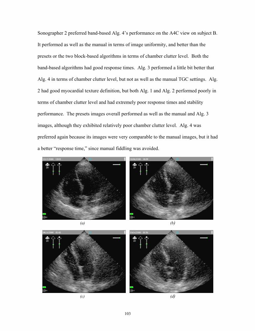
103
Sonographer 2 preferred band-based Alg. 4’s performance on the A4C view on subject B.
It performed as well as the manual in terms of image uniformity, and better than the
presets or the two block-based algorithms in terms of chamber clutter level. Both the
band-based algorithms had good response times. Alg. 3 performed a little bit better that
Alg. 4 in terms of chamber clutter level, but not as well as the manual TGC settings. Alg.
2 had good myocardial texture definition, but both Alg. 1 and Alg. 2 performed poorly in
terms of chamber clutter level and had extremely poor response times and stability
performance. The presets images overall performed as well as the manual and Alg. 3
images, although they exhibited relatively poor chamber clutter level. Alg. 4 was
preferred again because its images were very comparable to the manual images, but it had
a better “response time,” since manual fiddling was avoided.
(a) (b)
(c) (d)

104
(e) (f)
Fig. 7-13. Apical four chamber (A4C) view on large-frame, moderately difficult-to-image male subject (B) imaged by sonographer 2, generated with (a) manual TGC controls, (b) preset TGC controls, (c) Alg. 1, (d) Alg. 2, (e) Alg. 3, (f) Alg. 4.
For the SBC view on subject B, sonographer 1 found that the preset gain values, although
producing a uniform image, were on the whole just a little bit too low; thus, the preset
images were considered to have the lowest relative image quality. The block-based
algorithm images had relatively poor endocardial border clarity, and Alg. 1 images had
relatively poor chamber clutter level. Band-based Alg. 3 performed on par with the
manual gain settings in terms of myocardial texture definition and endocardial border
clarity, but its images exhibited a high chamber clutter level. Band-based Alg. 4 images’
myocardial border definition was as good as the manual images’, and Alg. 4 images also
had better chamber clutter level than the manual images. The manual and Alg. 4 images
were considered to have equivalent image quality, followed by Alg. 1 and Alg. 3 images,
and then Alg. 2 images.

105
7.2.1. Summary of Results
In summary, the differences between the performance of the different algorithms were
primarily aesthetic, not diagnostic. The sonographers’ feedback showed a definite
preference for the 16 radial band by 16 lateral band band-based control algorithm, Alg. 4.
Both of the block-based control approaches, Alg. 1 and Alg. 2, tended to produce overly
bright images that often had acceptable myocardial texture definition, but high chamber
clutter levels. They also frequently exhibited poor response time and stability, especially
with difficult-to-image Subject B. The 8 radial band by 8 lateral band band-based control
approach, Alg. 3, also tended to produce images with high chamber clutter level, but had
an acceptable response time and stability. Alg. 4 seemed to produce images of quality
close to the manual images, but due to its generally good response time and stability, was
preferred for its ease of use as compared to the manual TGC settings.
7.3. Analysis of Results These results correlate fairly well with the quantitative observations made. The near and
far band means shown in Fig. 7-2a and b show that the means are often fairly close to
each other for a given subject, imager and view, supporting the fact that most images
were of overall comparable image quality. The AGC algorithm near means are generally
a little bit greater than their respective manual near means. The AGC algorithm far
means tend to be slightly lower than their respective manual far means for views with
more myocardial content such as the parasternal long axis view, but a little bit higher for
views with more blood content, such as the apical four chamber view. The mean values
are fairly consistent between images taken of the same view on the same subject by

106
different sonographers. The few exceptions to these observations are the noted cases
where image quality was poor.
The observed gain settings provide some insight into the qualitative results. In general,
the overall gains set by the AGC algorithms are nearly always negative, resulting in AGC
overall gain values matching manual values well when the manual values are negative,
but not as well when the manual values are positive. The AGC-set near gains, on the
other hand, are generally positive values, suggesting that they are compensating for low
overall gains. They are, as a result, significantly higher than the manual near gain values.
The overall gain settings seem reasonable in general, except in cases like the subcostal
view on subject B, where block-based Alg. 1 and band-based Alg. 3 clearly produced
excessively high overall gain settings, but the near gain settings, especially those
produced by the block-based algorithms, are generally too high in comparison to the
manual gain settings. The overall gain settings, however, are generally lower, so the high
near gain settings implies that the near gain settings are merely compensating for the low
overall gain settings. The advantage of this approach to gain settings is that chambers in
the far field often appeared clearer in the algorithm-generated images than the manual
images, but because of the high near gain, chambers in the top of the near field often had
a very high chamber clutter level. Band-based Alg. 4 is the least aggressive of the
algorithms, thus taking on values less different from the manual ones that the other
algorithms, and more consistently producing good images.

107
The consistency of the gain settings of the different algorithms is another important
feature to consider. Looking at the overall gain settings for images of the same view on
the same subject but by different sonographers, we can note that Alg. 4 is the most
consistent, followed by Alg. 3. The block-based algorithms, Alg. 1 and Alg. 2, are not as
consistent; however, the variation is no greater than the interoperator differences in the
manual overall gain setting. In terms of near gain, Alg. 4 produced the most consistent
settings. The variation in the other algorithms’ settings, however, are not much greater
than the interoperator variation.
One of the most interesting results is that, although Alg. 4’s image quality often
surpassed the quality of images created using the preset gain settings, Alg. 4 often applied
the exact gain settings as the presets. (In at least one case, the subcostal view on subject
B, the preset gain settings were too low, and Alg. 4 did detect this situation and increased
the overall gain by 100; however, in most cases the presets and Alg. 4’s gain settings
were very similar.) This result suggests that a placebo effect exists; the sonographers are
more likely to like images that are created with some intelligence about the gain.
Another factor might be slight hardware variations in the transducers and systems used.
These possibilities can be evaluated by repeating the experiment with swapped
ultrasound systems and identifying the presets system as another AGC “algorithm”
system.
A few follow-up experiments (PLX and A4C views on Subject A with Sonographer 1)
were repeated using the two band-based algorithms, the presets and manual TGC’s,

108
exchanging the machines on which the algorithms were loaded previously. The preset
was disguised as a third AGC algorithm this time. The 16 radial band by 16 lateral band
band-based Alg. 4 was preferred over the 8 radial band by 8 lateral band band-based Alg.
3, and generally preferred over the presets, although as before, it generally set the gains
identically to the presets. The small sample set of trials explains why Alg. 4 was
sometimes preferred over the presets although their gain settings were similar. The
switched machines test at least eliminates the possibility that subtle machine differences
caused the good performance of Alg. 4 in the first set of clinical experiments, and
suggests that the results are due to a placebo effect.
The generally good performance of the presets and the similarity of the Alg. 4 and preset
gain settings suggest that the ideal AGC algorithm for a screening ultrasound device
should not be extremely aggressive. It only needs to detect cases where the gains are
egregiously off and correct for such a situation. Algorithms that are less aggressive also
lead to reproducible images; the gain settings are more likely to be similar between two
studies of the same patient, since the gain adjustments are not excessively sensitive.
The performance of the different algorithms indicates that band-based control is far more
successful than block-based control. Band-based control does imitate the user’s approach
more closely; on a traditional ultrasound machine there are 8 TGC controls that apply
different gains to 8 radial bands, and the user tries to optimize the gains for each band. In
the case of block-based control, the motion of the heart leads to the composition of blocks
changing over time, so that the target means for some blocks are likely to be wrong at any

109
given adjustment frame. The errors caused by movement are probably the chief
contributors to the instability and poor response times of the block-based algorithms, Alg.
1 and Alg. 2. This effect also probably overshadowed the effect of the choice of reset
mechanism.
The band-based approach, on the other hand, uses blocks only to define the composition
of a band more accurately; the general composition of a band is not as likely to change
with motion; for example, even if a valve moves up or down by a few centimeters, it will
still likely be within the band. Despite the poor gain settings of Alg. 3, which are likely
due to suboptimal parameter settings or insufficient granularity of classification, both it
and Alg. 4, the two band-based algorithms, exhibited good stability and response times.
The overall results suggest that AGC algorithms with band-based control show promise
as the basis for an automatic gain control on Agilent’s new ultrasound device.
110
Xk; rhap uhk;
8. Conclusions and Further Work 8.1. Conclusions of Current Investigation This investigation aimed to provide proof of concept of implementing automatic gain
control for a 2D cardiac ultrasound screening tool, and it has shown that achieving AGC
is feasible, and it will indeed be a useful feature. In sharp contrast to the reaction of users
to AGC on high performance ultrasound devices, the response of sonographers who
evaluated AGC on Agilent’s portable device was extremely favorable. The feature was
considered a useful addition that speeded up image acquisition. These results support the
hypothesis that the role of AGC is different on a screening device than a high-
performance ultrasound scanner; shortness of study is most important on a screening
device whereas impeccable image quality is most important on a diagnostic device. The
primary purpose of AGC on a screening device is to correct the gains if the preset values
are extremely inappropriate, rather than to improve image quality.
The results of this investigation indicate that a generic approach to automatic gain
control, such as classification-based AGC algorithms are far more successful than a
specific, knowledge-based approach such as view-based AGC algorithms. The
performance of prototype band-based control classification-based AGC algorithms
suggest that such simple approaches to AGC can be developed as a viable commercial
implementation.

111
8.2. Further Experiments Further clinical experiments must be performed to validate the findings of this
investigation. At a minimum, the algorithms should be tested with more sonographers,
subjects and views. For example, how well do the algorithms perform when imaging a
carotid artery or a pediatric patient? The algorithms should be tested for imaging patients
with more serious pathologies as well to ascertain that it is effective in a device used as a
screening tool. More implementations of the band-based control AGC algorithms should
also be evaluated using different parameter values, to find the optimal values that produce
the best performance.
Another extremely important set of experiments to perform involve the testing of the
AGC algorithms using novice users. Algorithms which produce images of good quality
should be tested with inexperienced imagers to determine how useful they find AGC.
Another consideration is to determine how well the algorithms perform with a novice
user. For example, an experienced user can detect cases where the gains are not
optimally set and adjust the transducer to trigger an AGC reset; a novice user is more
likely to rely completely on the machine’s settings. These experiments are necessary to
demonstrate the usefulness of an AGC feature to inexperienced users.
8.3. Possible Additional Developments 8.3.1. Improvements to Classification Once the results of this investigation are confirmed by further experiments, attention
should be given to develop the classification-based AGC algorithm in order to improve

112
its performance. One half of this effort entails improving the classification step of the
algorithm, to arrive at a more accurate estimate of the composition of a band. The
simplest improvement is to average the data from several frames to arrive at the target
band means.
The use of variance to aid in classification should perhaps be revisited. Although
variance proved to be a poor indicator of the composition of a block, it may be a good
measure of the degree of bimodality in the set of samples in a block. A better knowledge
of the extent of bimodality in a block could be used to classify blocks into additional
categories, such as “mostly blood,” “tissue with blood” or “tissue with specular.” Using
such classifications for the composition types of a block would result in the definition of
more specific ideal means, and a more accurate target band mean.
Changing the granularity at which the classification occurs could improve performance,
For example, the target band means could be computed using data at the sample level.
Each sample in a band could be classified as blood, tissue or specular, and these values
could be averaged to determine the appropriate target mean for the block. This approach
would require a re-evaluation of appropriate relative value and target value (relative and
target mean for a block) parameter values. One caution to this approach, however, is that
the number of comparisons could possibly be so computationally intensive that the frame
rate could be reduced. Using smaller blocks, such as those in a 32 by 32 grid, may be a
more effective way of improving classification. Using variable sized blocks—larger ones
in the near field and smaller ones in the far field—may also have an impact. Since the

113
acoustic data set is in polar coordinates, a block of data in the near field contains far more
samples per area than a block of the same size in the far field.
8.3.2. Improvements to Control Improvements to the response time, correctness and stability of the AGC algorithms is
crucial to the success of automatic gain control in a screening device. Novice users will
depend on the correctness of the machine’s settings, especially as they learn to use the
device. The most important area to explore is a revision of the AGC reset system.
Currently, the system will leave the gains values static if the image band means have not
changed much from the previous frame. This approach does not self-correct for cases
where the gains might have been mis-set. A more robust option would be to reclassify
the image every several frames, and automatically adjust the gains. The frequency of re-
classification will be highly dependent on how this relatively computationally intensive
step affects the frame rate. The characterization tests have shown that the classification
scheme works well at non-initial gain settings, so it would probably be feasible to have
alternating classification and gain adjustment phases without any explicit reset to the
initial default values.
Another important area to investigate is deciding which data samples affect which gain
settings, and to what degree they have an effect. For example, of the samples that
comprise the near band in the current algorithm implementation, about 2/3 of the samples
only have a fraction of the near gain applied to them, since the near gain is linearly
ramped to zero. On the other hand, the samples in the top fourth of the field, which are
ignored, have the entire near gain applied to them. Some sort of weighting factor should

114
perhaps be considered so that samples that have the entire near gain value applied to them
should have more effect on the adjustment of the near gain than samples that have only a
fraction of the near gain applied to them. A simpler solution would be to optimize the
probe compensation curves for the automatic gain control algorithms; for example, if the
top fourth of the image is known to be mostly noise and appears too bright with the AGC
controls, the probe compensation curve could contain lower gains in the very top of the
near field.
A related set of improvements involves the use of automatic gain control to improve the
image quality. To control the gains manually at smaller step sizes is impractical, since it
would slow down the amount of time to reach the appropriate gain levels. AGC
algorithm does not have this restriction; the current implementations indeed use an
adjustment granularity of 20, which is a fifth of the manual granularity of 100. A reliable
AGC algorithm could potentially use this finer degree of control to produce better
images. Adding extra gain control buttons, such a mid gain control setting, would
increase the complexity of the user interface, although it could generate better images.
Increasing the temporal (spatial) granularity of gain control is a straightforward extension
to the classification-based AGC algorithm, however. This addition could possibly
improve image quality in many cases, for example, in cases where the top fourth of the
image is too noisy, but the rest of the near field is slightly dim.

115
8.4. Conclusion
Given the results of this investigation, automatic gain control holds promise as a feature
on Agilent’s small portable ultrasound device that will increase efficiency for
experienced users and perhaps increase simplicity and ease for novice users. For AGC to
be a viable feature on a device, it will be necessary to develop automatic gain control for
Doppler color flow mapping as well, a crucial technique in cardiac ultrasound imaging
that depicts the velocity of blood flow. Among the prototype 2D cardiac ultrasound AGC
algorithms, one has been demonstrated to be responsive and accurate. If this algorithm is
further developed along the lines described above, the successful implementation of
automatic gain control for a cardiac ultrasound screening tool seems very likely.

116
References Alexander, C., Dinh, B., Fallon, J. and Mucci, R. “A ‘Simplified’ Time Gain Control
Technique.” October 16, 1995. Agilent Techonologies. DeClercq, Andre, and Maginness, Max G. “Adaptive Gain Control for Dynamic
Ultrasound Imaging.” 1975 Ultrasonics Symposium Proceedings, IEEE, 1975; 59-63.
Hughes, David I., and Duck, Francis A. “Automatic Attenuation Compensation for
Ultrasonic Imaging.” Ultrasound in Medicine and Biology, 1997; 23,5:651-64. Hunt, Barry F., Leavitt, Steven C., and Hempstead, David C. “Digital Processing Chain
for a Doppler Ultrasound System.” Hewlett-Packard Journal, June 1986; 45-8. Hussey, Matthew. Basic Physics and Technology of Medical Diagnostic Ultrasound.
New York: Elsevier, 1985. Inbar, Dan and Delevy, Moshe. U.S. Patent 4,852,576. “Time Gain Compensation for
Ultrasonic Medical Imaging Systems.” August 1989. Karrer, H. Edward, and Dickey, Arthur M. “Ultrasound Imaging: An Overview.”
Hewlett-Packard Journal, October 1983; 3-6. Leavitt, Steven C. U.S. Patent 4,750,145. “Doppler AGC Using Overflow Counters
Internal to FFT.” June 1988. Maginness, Maxwell G. “Methods and Terminology for Diagnostic Ultrasound Imaging
Systems.” Proceedings of the IEEE, April 1979; 67,4:641-53. McDicken, W.N., Evans, D.H., Robertson, D.A.R. “Automatic Sensitivity Control in
Diagnostic Ultrasonics.” Ultrasonics, 1974; 173-6. Melton, Jr., Hewlett E., Skorton, David J. “Rational Gain Compensation for Attenuation
in Cardiac Ultrasonography.” Ultrasonic Imaging, 1983; 5:214-28. Mo, Larry Y.L. European Patent No. 1 005 833. “Method and Apparatus for Automatic
Time and/or Lateral Gain Compensation in B-mode Ultrasound Imaging.” June 2000.
O’Donnell, Matthew. “Quantitative Volume Backscatter Imaging.” IEEE Transactions
on Sonics and Ultrasonics, January 1983; 30,1:26-36. Pincu, Madeleine, et. al. “Attenuation Correction in Echocardiography.” Ultrasonic
Imaging, 1986; 8:86-106.

117
Pye, S.D., Wild, S.R. and McDicken, W.N. “Adaptive Time Gain Compensation for Ultrasonic Imaging.” Ultrasound in Medicine and Biology, 1992; 18,2:205-12.
Rose, Joseph L. and Goldberg, Barry B. Basic Physics in Diagnostic Ultrasound. New
York: Wiley, 1979. Snyder, Richard A. and Conrad, Richard J. “Ultrasound Image Quality.” Hewlett-
Packard Journal, October 1983; 34-8.

118
Acknowledgements This thesis project was carried out at the Imaging Systems Division of Agilent Technologies’ Healthcare Solutions Group. I am extremely grateful to Agilent Technologies and to the engineers there who have guided me through this project. I especially thank my manager, Benjamin Herrick, for his cooperation and support, and Steven C. Leavitt, for the patient and valuable technical supervision he has provided during the course of my thesis research. I thank clinical specialist Donna Rubosky for helping me to collect all the necessary data for analysis, and her and Lorraine Henderson for assisting with the clinical evaluations. I also thank all the members of the OptiGo team at Agilent for their perpetual encouragement and readiness to help. My gratitude also extends to Dave Prater, David Clark, Robert Arnold, Gary Dallas, Bernie Savord and Ron Hudgens, were always available to answer my questions, or to discuss ideas. The opportunities and support provided by Agilent to me were invaluable. I also thank my MIT thesis supervisor, Prof. Martha Gray, of the Harvard-MIT Division of Health Sciences and Technology for her feedback on my thesis work.