AUTOMATIC GENERATION OF BOUNDARY CONDITIONS USING DEMONS

NON-RIGID IMAGE REGISTRATION FOR USE IN 3D MODALITY-

INDEPENDENT ELASTOGRAPHY

By

Thomas S. Pheiffer

Thesis

Submitted to the Faculty of the

Graduate School of Vanderbilt University

in partial fulfillment of the requirements

for the degree of

MASTER OF SCIENCE

in

Biomedical Engineering

May, 2010

Nashville, Tennessee

Approved:

Professor Michael I. Miga

Professor Robert L. Galloway

ACKNOWLEDGEMENTS

I would like to thank my advisor Dr. Michael Miga for his guidance and Dr. Jao Ou for all of his advice and development of the algorithm which forms the basis for this work. I am also grateful to the rest of the members of the BML and SNARL labs for their friendship and support, particularly Rowena Ong in sharing her data and Dr. Amber Simpson for her advice. I would also like to thank the Vanderbilt Medical Center CT department for the scans of our phantoms, as well as Dr. Thomas Yankeelov and Dr. John Boone (University of California-Davis Medical Center, Dept. of Radiology) for the human breast MR and CT data sets, respectively.

ii  

TABLE OF CONTENTS

Page ACKNOWLEDGEMENTS ................................................................................................ ii

LIST OF TABLES ............................................................................................................. iv

LIST OF FIGURES ............................................................................................................ v

LIST OF ABBREVIATIONS ........................................................................................... vii

Chapter I. INTRODUCTION ........................................................................................................ 1

1.1 Motivation ................................................................................................................. 1 1.2 Previous Work ........................................................................................................... 3

II. METHODOLOGY ....................................................................................................... 6 2.1 MIE Workflow .......................................................................................................... 6 2.2 Automatic Generation of Boundary Conditions........................................................ 8 2.3 Simulations ................................................................................................................ 9 2.4 Phantom Experiment 1 ............................................................................................ 10 2.5 Phantom Experiment 2 ............................................................................................ 12

III. RESULTS .................................................................................................................. 17 3.1 Simulations .............................................................................................................. 17 3.2 Phantom Experiment 1 ............................................................................................ 22 3.3 Phantom Experiment 2 ............................................................................................ 23

IV. DISCUSSION ............................................................................................................ 29 4.1 Simulations .............................................................................................................. 29 4.2 Phantom Experiment 1 ............................................................................................ 32 4.3 Phantom Experiment 2 ............................................................................................ 34

V. CONCLUSION .......................................................................................................... 38

REFERENCES ................................................................................................................. 40

iii  

LIST OF TABLES

Table Page

1. Comparison of boundary condition mapping error and MIE reconstruction results between the four methods. The boundary error was calculated against known boundary conditions, and the MIE reconstructions were compared against the known contrast ratio of 6:1. .................................................................................. 20

 

2. Comparison of boundary condition mapping error for Phantom 1, Phantom 2, and Phantom 3. The error was calculated against the localized positions of fiducial beads in the source and target images. .................................................................. 26

 

3. Comparison of the MIE-reconstructed elasticity contrast ratios for Phantom 2 and Phantom 3 when using TPS and demons boundary conditions, as well as the mean contrast observed via material testing of the gels. ................................................ 27

iv  

LIST OF FIGURES

Figure Page

1. Overview of the MIE protocol. The boundary condition task is seen to be in a central location and has a critical impact on the final reconstruction. .................... 7

2. Source CT mesh (a) with cross-section showing tumor-to-normal elasticity contrast (b), and source MR mesh (c) with cross-section showing similar contrast (d). ......................................................................................................................... 10

3. Representative slices from the two data sets used for the simulations. Slice (a) shows the CT image in its pre-deformed state, and (b) shows the CT image in its post-deformed state. Slice (c) shows the MR image in its pre-deformed state, and (d) is the MR image in its post-deformed state. .................................................... 17

4. Source CT mesh (a) and simulated target CT mesh (b), where the colorbar refers to the magnitude of the displacement applied by the known boundary conditions to result in the target. Source MR mesh (c) and simulated target MR mesh (d) similarly shown. .................................................................................................... 18

5. TRE distribution (in mm) across the surfaces of the CT mesh (a) and the MR mesh (b) for the demons-based boundary conditions compared to the known conditions. ............................................................................................................. 19

6. Objective function maps for the CT simulation (a) and the MR simulation (b). The objective function value calculated by the optimization framework is plotted on the ordinate axis against selected elasticity contrast ratios (tumor-to-normal) as affected by the boundary conditions. Shown are the objective maps of the demons case (solid lines) and the known boundary conditions as the control (dashed lines). The ordinate is scaled in both cases. .......................................................... 21

7. Surface renderings and representative slices from Phantom 1 at each state of deformation. This phantom exhibits little contrast and contains no tumor, and so was used only for testing boundary condition accuracy instead of a full MIE reconstruction. The figures in (a) and (b) display the phantom with no

v  

compression, (c) and (d) display the phantom under 50% compression, and (e) and (f) display the phantom under 100% compression. ........................................ 22

8. Surface renderings and representative slice of Phantom 2 while pre-deformed (a,b), and while under 100% compression (c,d). .................................................. 24

9. Surface renderings and representative slice of Phantom 3 while pre-deformed (a,b), and while under 100% compression (c,d). .................................................. 25

10. Objective function maps for Phantom 2 (a) and the Phantom 3 (b). The objective function value calculated by the optimization framework is plotted on the ordinate axis against selected elasticity contrast ratios (tumor-to-normal) as affected by the boundary conditions. Shown are the objective maps of the demons case (solid lines) and the TPS boundary conditions as the control (dashed lines). The ordinate is scaled in both cases. .......................................................................................... 28

   

vi  

vii  

LIST OF ABBREVIATIONS

Abbreviation Full Name

1. TPS Thin-plate spline

2. MIE Modality-independent elastography

3. FEM Finite element method

4. BC Boundary conditions

5. SCP Symmetric closest point

6. TRE Target registration error

7. PDE Partial differential equation

8. MR Magnetic resonance

9. CT Computed tomography

10. w/v Weight per volume

CHAPTER I

INTRODUCTION

1.1 Motivation

Breast cancer is second only to lung cancer in cancer-induced mortality among

women. The American Cancer Society estimated that in 2009, over 194,000 new cases of

invasive breast cancer would be diagnosed, in addition to over 62,000 cases of in situ

breast cancer, and an estimated 40,000 deaths from the disease that year. Additional

statistics underscore the importance of early initiation of treatment, as the five-year

relative survival rates for women diagnosed with breast cancer are only approximately

27% for advanced distant-stage disease, but are as high as 98% for early localized disease

(ACS 2009). In addition, tumor size has been directly correlated to prognosis of 5- to 10-

year survival, and has significant implications for long-term survival (Michaelson,

Silverstein et al. 2002; Warwick, Tabar et al. 2004). Early detection is therefore both an

inherently desirable goal and one which presents demands for more sensitive detection

techniques.

Breast cancer lesions have traditionally been detected clinically by palpation and

imaging modalities such as X-ray mammography. Palpation allows for the qualitative

contrast of diseased tissue from normal tissue by recognizing that cancerous lesions are

generally firmer to the touch than normal tissue. This allows for identification of regions

that may require biopsy for histological examination. However, palpation suffers from

having a short depth of detection into the tissue, and is subjective in nature.

1  

Mammography, while being the standard technique for breast screening, has been shown

to have questionable reliability when used in isolation (Keith, Oleszczuk et al. 2002).

An alternative imaging methodology that, like palpation, utilizes the mechanical

properties of tissue is known as elastography. Elastography employs a combination of

image processing and measurements of the physical deformation of the tissue to create a

representation of the mechanical strength of structures inside the breast (Bilgen 1999;

Doyley, Meaney et al. 2000). The overall principle behind elastography for use in breast

cancer imaging is that regional changes in tissue architecture resulting from the

manifestation of disease result in detectable changes in mechanical properties. It is

widely recognized in the medical community that most breast cancers are much firmer to

the touch than the surrounding soft tissue. The biological basis for this effect is due to

changes in tissue composition, such as varied expression of collagen and greater numbers

of fibroblasts (Burns-Cox, Avery et al. 2001; Lee, Sodek et al. 2007). The exploitation of

a contrast mechanism based on elastic properties may have considerable potential as

means for characterization of disease states.

Several kinds of elastography exist, such as ultrasound elastography (USE) and

magnetic resonance elastography (MRE) which have already shown promise in

diagnosing solid lesions in breast tissue and other physiological locations. The first

introduction of USE demonstrated that images from A-line ultrasound could provide

axial strain estimates (Ophir, Cespedes et al. 1991). Elastography has also been applied

within the MR imaging domain whereby motion-sensitized gradient sequences were used

to visualize and quantify strain wave propagation in media (Muthupillai, Lomas et al.

1995). A relatively new method known as modality-independent elastography (MIE) has

2  

recently shown potential for supplementing other imaging modalities such as MR and CT

for detection of solid tumors in soft tissue (Miga 2003).

MIE has the benefit of being flexible with regard to its inputs, and unlike USE

and MRE, it is not reliant on a particular imaging modality. MIE involves imaging a

tissue of interest before and after compression, and then applying a finite element (FE)

soft-tissue model within a nonlinear optimization framework in order to determine the

elastic properties of the tissue. A requirement of the MIE method is that appropriate

boundary conditions be designated for use in the biomechanical model. Generation of

accurate boundary conditions is problematic because the breast is a non-rigid structure,

which invalidates the use of standard rigid registration techniques. Techniques which

have addressed this issue in the past have required a significant amount of user

interaction. The goal of this work is to develop and validate a method of generating

boundary conditions automatically by registering breast surfaces before and after

mechanical loading. This method may have potential not only in MIE, but also in other

applications requiring registration of breast surfaces.

1.2 Previous Work

The methods used for registering breast images generally fall into one of two

broad categories: 1) feature-based methods or 2) intensity-based methods (Guo,

Sivaramakrishna et al. 2006). Feature-based methods utilize geometric information from

the images, such as from an FE mesh of the breast structure, to register two breast

images. Intensity-based methods instead directly use the intensity values of the image

voxels, and optionally some geometric information, to register the two images.

3  

The previous gold standard in generating boundary conditions for MIE has been

feature-based registration methods (Ou, Ong et al. 2008). Conventionally this entails

employing point correspondence methods facilitated by attached fiducials and assisted by

thin-plate spline (TPS) interpolation (Goshtasby 1988) to create the boundary conditions

that non-rigidly maps the pre-deformed breast surface to the post-deformed breast

surface. This registration process requires the tedious task of applying and subsequently

localizing numerous surface markers within the image space, determining point

correspondence, creating a thin-plate spline interpolation, and finally calculating a set of

Dirichlet boundary conditions for use in the MIE method. Initial attempts to reduce the

complexity and level of user interaction have focused on the use of two energy

minimization techniques (Ong, Ou et al. 2010). These techniques relied upon partial

differential equation (PDE) solutions of Laplace’s equation,

· Φ 0, (1)

or the diffusion equation,

Φ · Φ , (2)

across the surface of the breast geometry in the pre- and post-deformed states. Like-

valued isocontours from the solutions on each surface (i.e. pre-deformed, and post-

deformed) act as ‘virtual’ fiducials to assist in correspondence using a symmetric closest

point approach (Papademetris, Sinusas et al. 2002). Dirichlet boundary conditions are

generated after the assigned correspondence is determined and this completes the

required input for the MIE algorithm. The primary difference between the two

methodologies is the boundary condition requirement and subsequently the required

degree of user interaction. For the Laplacian method, Dirichlet boundary conditions were

4  

required to be assigned to two distinct regions of the mesh surface (points along the chest

wall, and nipple were assigned potential values of 1 and 0, respectively, with unity

conductivity). For the diffusion method, only one distinct region need be designated (in

this case an initial condition of zero potential was supplied, with a unity Dirichlet

condition assigned at the nipple). While the results presented by Ong et al. (2010)

indicated better performance via the Laplacian method, the diffusion method did not

require the difficult task of assigning a boundary condition to the chest wall in both pre-

and post-deformed mesh domains. These methods, as well as the TPS method, will be

compared to the intensity-based approach in this paper.

While the above PDE-based methods represented an improvement in automation

over the TPS method for generating boundary conditions for the MIE algorithm, the ideal

boundary condition method would be both fully automated and require no fiducials. This

study presents an approach for automatically generating boundary conditions through the

use of a popular non-rigid image registration algorithm called demons diffusion. The

demons algorithm was used to perform image matching of pre- and post-deformation

images and tested against a controlled in silico simulation with known boundary

conditions. The generated boundary conditions were also used to perform an MIE

elasticity reconstruction to evaluate its effectiveness in determining the elasticity contrast

of a previously characterized system. The simulation study was followed by two phantom

experiments to further stress the abilities of this new approach.

5  

CHAPTER II

METHODOLOGY

2.1 MIE Workflow

As described in previous work, the MIE algorithm is comprised of three major

components: 1) a biomechanical FE model of soft-tissue deformation based on material

properties, 2) a similarity metric with which to compare images, and 3) an optimization

routine to update the material properties in the model (Miga, Rothney et al. 2005).

The process of generating an elasticity reconstruction begins with the acquisition

of an image of the breast. A mechanical load is then applied to the breast, and the breast

is imaged again. These pre- and post-deformation images comprise the primary input to

the MIE algorithm, and are referred to as the source and target images, respectively. The

breast boundary is then segmented in the pre-deformed source image and its surface

geometry is extracted using the marching cubes algorithm, which allows a finite element

mesh to be created from the surface information. The mesh is partitioned into 'regions' to

which elasticity properties are assigned, which defines the resolution of the elastographic

reconstruction. It is then necessary to designate the loading/boundary conditions for the

FE model. The ability of the biomechanical model to accurately deform the mesh of the

breast tissue is dependent on these boundary conditions. The boundary condition step in

the MIE workflow is highlighted in Figure 1.

6  

 

Figure 1. Overview of the MIE protocol. The boundary condition task is seen to be in a central location and has a critical impact on the final reconstruction.  

Once boundary conditions have been designated, the model is run and the FEM

displacement solution for all the nodes in the mesh is obtained. The displacements are

then used to deform the original pre-deformation image, which is then compared with the

known post-deformation image to generate an image similarity measurement. A non-

linear optimization framework is used to update the material properties of the mesh until

the similarity metric is within tolerance, at which point the elasticity reconstruction image

is produced.

7  

2.2 Automatic Generation of Boundary Conditions

The demons registration algorithm utilizes a diffusion model in which the object

boundaries in one image are characterized as semi-permeable membranes, and the other

image is allowed to diffuse through these membranes (Thirion 1998). Following the

formulation of Ibanez, et al.(Ibanez, Schroeder et al. 2005),

D X · X m X f X (3)

where f(X) is the fixed target image, m(X) is the source image being deformed for the

registration, and D(X) is the displacement field mapping the source to the target image

through an instantaneous optical flow. The algorithm used in this work was based on the

Insight Toolkit (Yoo, Ackerman et al. 2002), which reformulated Equation 3 to an

algorithmic iterative form as follows:

DN X DN-1 Xm X DN-1 X f X f X

f m X+DN-1 X f X

(4)

The displacement field obtained from Equation 4 is smoothed with a Gaussian

filter between each iteration in order to enforce elastic-like behavior. This aspect of the

algorithm’s implementation made it appropriate for modeling the boundary conditions of

a system being deformed within the confines of an elastic model.

The registration produces displacements at the centroid of every voxel. The

displacement vectors are then interpolated onto the nodal coordinates of the FE mesh

using a cubic 3D interpolation. The displacements which are assigned to boundary nodes

are thus designated as the Type I boundary conditions for the elastic model.

8  

2.3 Simulations

In order to evaluate the demons method of generating boundary conditions for

MIE as described above, a controlled experiment was conducted by obtaining a CT and

an MR image volume of human breast tissue and registering them to target images

created by simulated mechanical loads.

Two image sets (CT and MR) of normal tumor-free human breast tissue were

obtained from the UC-Davis Department of Radiology and the Vanderbilt University

Institute of Imaging Science, respectively, for use in this work. The surface of each breast

image was segmented from the surrounding structures with ANALYZE 8.1 (Mayo

Clinic, Rochester, MN) and the resulting segmentation was used to create a 3D FE mesh

using a tetrahedral mesh generation algorithm (Sullivan, Charron et al. 1997). For both

the CT set and the MR set, a 2-cm spherical tumor was synthetically implanted in the

center of the respective mesh and assigned an elasticity value six times higher than the

surrounding material, which is consistent with breast cancer elasticity contrasts in the

literature (Krouskop, Wheeler et al. 1998). This contrast ratio of 6:1 was thus considered

to be the goal for reconstruction in both cases. The location of the tumor in each mesh is

visualized in Figure 2.

9  

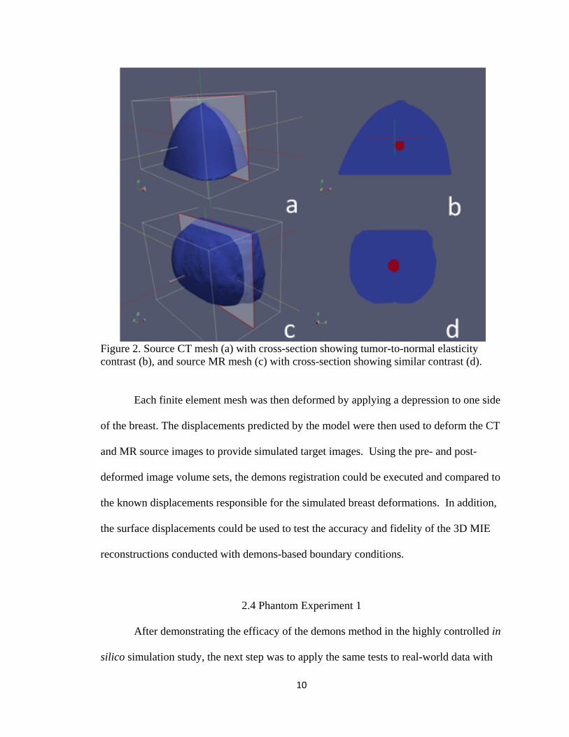
 Figure 2. Source CT mesh (a) with cross-section showing tumor-to-normal elasticity contrast (b), and source MR mesh (c) with cross-section showing similar contrast (d).

Each finite element mesh was then deformed by applying a depression to one side

of the breast. The displacements predicted by the model were then used to deform the CT

and MR source images to provide simulated target images. Using the pre- and post-

deformed image volume sets, the demons registration could be executed and compared to

the known displacements responsible for the simulated breast deformations. In addition,

the surface displacements could be used to test the accuracy and fidelity of the 3D MIE

reconstructions conducted with demons-based boundary conditions.

2.4 Phantom Experiment 1

After demonstrating the efficacy of the demons method in the highly controlled in

silico simulation study, the next step was to apply the same tests to real-world data with

10  

realistic amounts of noise and uncertainty. To this end, breast phantom images were

acquired to evaluate the ability of the demons method to produce accurate boundary

conditions when compared to the current gold standard method.

As described by Ong et al. (2010), the breast phantom used in this study

(hereafter referred to as Phantom 1) was created from an 8% w/v solution of polyvinyl

alcohol (Flinn Scientific, Batavia, IL). The gel was frozen in a breast-shaped mold at -

37°C for 16 hours and then allowed to thaw at room temperature to produce a tissue-

mimicking breast phantom. To provide intrinsic fiducial markers, thirty-four 1-mm

stainless steel beads were distributed over the phantom directly under its surface. It

should be noted that, except for the beads, there was little to provide intensity

heterogeneity within this phantom. A mechanical load was applied to the phantom in a

custom-built acrylic chamber via a neoprene sphygmomanometer air bladder (W.A.

Baum, Copiague, NY) positioned on the side of the phantom. This compression device

was constructed so that an adjustable wall could be positioned to hold the phantom in

place, while on the opposite side the air bladder was located approximately at the

midpoint of the height of the phantom.

The phantom was subjected to three levels of compression by inflation of the air

bladder: no compression, inflation with 50% of the maximum bladder pressure, and full

inflation of the bladder. At each state of compression, CT images were acquired with

dimensions 512 x 512 x 174, and 0.54 x 0.54 x 1 mm voxel size. The images were then

segmented and triangular meshes were created from the surface geometry of the

phantom. The uncompressed mesh was composed of 8,127 nodes, the 50% compression

mesh was composed of 6,777 nodes, and the 100% compression mesh was composed of

11  

8,260 nodes. From the meshes, the fiducial bead centroid positions were localized and

then used in a TPS interpolation to provide the gold standard boundary conditions for two

scenarios: 1) deforming from the uncompressed state to the 50% compression state, and

2) deforming from the uncompressed state to the 100% compression state. In generating

the TPS boundary conditions, 33 of the beads were used in calculating the interpolation,

while the last fiducial was used to evaluate the target registration error (TRE). In an effort

to evaluate the error over the entire surface, the TPS registration was conducted 34 times,

each time using a different fiducial for the TRE calculation. The final TRE for the TPS

gold standard was the average of these repetitions. The demons method was then used

independently to generate boundary conditions mapping from the pre- to the post-

deformed surface of the breast phantom for the two scenarios, and compared to the

control TPS result, as well as previous semi-automated methods (Laplace equation and

diffusion methods). The registration in both scenarios utilized 120,000 iterations and a

Gaussian smoothing kernel standard deviation of 1.5.

2.5 Phantom Experiment 2

Following the evaluation of the performance of the demons method in generating

boundary conditions in the above phantom study, a second phantom experiment was

designed to test the performance of demons-based boundary conditions in the context of a

full MIE reconstruction. Two more phantoms (hereafter referred to as Phantom 2 and

Phantom 3) were constructed of polyvinyl alcohol cryogel (PVA-C) to test the accuracy

of the reconstruction when validated with material testing data.

12  

As described by Ou, the two new phantoms were created with a 7% w/v

suspension of hydrolyzed polyvinyl alcohol powder heated to 80°C, which was then

incorporated with 10% glycerol (Fisher Scientific, Pittsburgh, PA) by volume (Ou 2008).

Due to the nature of the polymerization of the gel, sequential freeze-thaw cycles (FTCs)

achieve varying levels of stiffening elasticity. A FTC in this study was defined as

bringing the gel down to -37°C over the course of 12 hours and then allowing it to return

to room temperature over the next 12 hours.

The two phantoms were constructed by first mixing the components described

above. To test the ability of the MIE algorithm, there needed to be a detectable difference

in the elasticity between the phantom tumor and the rest of the phantom breast. In order

to make the tumor stiffer than the normal tissue, the bulk of the phantom was subjected to

one FTC, while the tumor underwent two FTCs. The tumor was made in a 25-mm

diameter spherical mold for its first FTC, and was then suspended with very thin plastic

wires approximately in the center of the mold used to simulate the shape of a pendant

breast. While the FTCs produce elasticity contrast between the tumor gel and normal gel,

it does not produce an appreciable CT image contrast between the two materials to enable

the MIE similarity metric to detect differences in the deformed images. In order to

introduce more contrast into the images, a small amount of radiopaque contrast was

initially added to the tumor mixture in the form of a 6% v/v quantity of barium sulfate

suspension (Lafayette Pharmaceuticals, Lafayette, IN). Prior to the second FTC, a 3% v/v

barium sulfate mixture was injected into the bulk breast gel in a few random streams to

improve the overall image texture. The second FTC then proceeded and the wires

suspending the tumor were removed to produce the final anthropomorphic breast

13  

phantom containing a stiff tumor. Similar to the first phantom study,

polytetrafluoroethylene spherical beads (McMaster-Carr, Atlanta, GA) with a 1.6-mm

diameter were distributed just under the surface of the phantoms in order to facilitate a

TPS interpolation to act as the gold standard boundary conditions. Phantom 2 received 35

beads, while Phantom 3 received 32 beads. The TRE for the TPS registration was

calculated using a ‘leave-one-out’ strategy similar to the approach described in the first

phantom experiment.

In order to evaluate the performance of MIE when using the demons-based

boundary conditions, validation was needed for the material property contrast between

the tumor and normal gel. To achieve this, independent mechanical tests were performed

on samples of the two gel elasticity constituents of the phantom. A sample from each gel

(tumor and normal) was set aside for this testing during fabrication. Each was poured into

standard 24-well polystyrene cell culture plates (Corning Inc. Corning, NY) and

subjected to its respective number of FTCs. This process resulted in cylindrical gel

samples with diameter and height both about 15 mm, which could then be subjected to

compression testing using an ElectroForce 3100 material tester (Bose, Eden Prairie, MN).

The instrument was programmed to provide fixed displacements to the cryogels when the

samples were mounted on a platform over a 22.5 N load cell. Each sample was subjected

to five cycles of a load rate of 0.15 mm/s and then held for 300 s for strains of 2, 5, 10,

and 15% in compliance with small deformation theory. Average elastic modulus values

for the two gels were obtained from the slope of the stress-strain curves of the steady-

state loading phases.

14  

The two phantoms were constructed with tumors located at varying distances

from the surface being compressed. The maximum diameter at the base of both phantoms

was approximately 105 mm. The Phantom 2 tumor was approximately 12 mm below the

surface, while the Phantom 3 tumor was approximately 26 mm below the surface. The

phantoms were imaged in the previously described air bladder chamber using a CT

scanner (Philips Medical, Bothell, WA). The Phantom 2 CT images (pre- and post-

deformation) were reconstructed with dimensions of 512x512x143 and voxel spacing of

0.27 x 0.27 x 0.8 mm, while the Phantom 3 CT images were reconstructed with

dimensions of 512x512x139 and voxel spacing of 0.26 x 0.26 x 0.8 mm.

The pre-deformed source image volumes were segmented from the compression

chamber and their surface information was used to create tetrahedral meshes. The

Phantom 2 mesh was constructed of 30,900 nodes and 166,509 elements, while the

Phantom 3 mesh was constructed of 33,930 nodes and 183,609 elements. The TPS

boundary conditions were generated using the implanted beads as control points for a

thin-plate spline interpolation between the pre- and post-deformation surfaces for each

phantom set. The PDE-based and demons methods were then utilized to independently

generate boundary conditions for the two phantoms. The demons registration was set to

run for 30,000 iterations for these sets, with a Gaussian smoothing kernel standard

deviation of 1.5.

The accuracy of the demons-based boundary conditions could then be evaluated

by comparing the gold standard TRE of the TPS method, the TRE of the PDE-based

methods, and the TRE of the points when used in the demons method. The

appropriateness of demons-based boundary conditions was then tested by employing

15  

them in a MIE reconstruction comparing elastic modulus values to independent

measurements. To constrain the problem, only two regions of material properties were

designated in the mesh: the tumor and the bulk normal gel. A priori knowledge of the

location of the tumor was also used by segmenting the tumor margins from the normal

gel beforehand in order to assign the material types to their corresponding elements in the

FE model. The results of the MIE reconstruction using demons-based boundary

conditions were also compared to the results of the reconstruction when using TPS

boundary conditions, and those derived from the PDE methods. The Poisson’s ratio used

in the model for both experiments was 0.485 to approximate an incompressible tissue-

mimicking material.

16  

CHAPTER III

RESULTS

3.1 Simulations

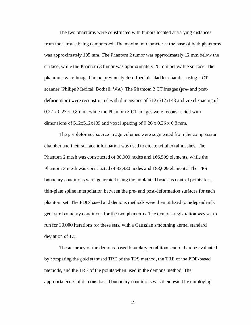
The CT and MR image source images were acquired and then deformed with the

set of known boundary conditions as shown below in Figure 3.

 Figure 3. Representative slices from the two data sets used for the simulations. Slice (a) shows the CT image in its pre-deformed state, and (b) shows the CT image in its post-deformed state. Slice (c) shows the MR image in its pre-deformed state, and (d) is the MR image in its post-deformed state.  

Figures 3a and 3b show an axial slice from the pre-deformed (left) and post-deformed

(right) CT image volume, respectively. Figures 3c and 3d show a pre-deformed (left) and

post-deformed (right) slice from the MR image volume, respectively.

17  

The deformations applied in both cases were approximately Gaussian in

distribution across the depressions as shown in Figure 4 below. The maximum

displacement experienced by the CT set was approximately 13 mm and was applied to

the side of the source CT mesh (Figure 4a) to result in the target post-deformed mesh

(Figure 4b) which was used to create the simulated target image for this experiment. The

MR mesh was similarly deformed by applying an approximately 12 mm depression to the

top of the source MR mesh (Figure 4c) to result in the simulated MR mesh (Figure 4d).

 Figure 4. Source CT mesh (a) and simulated target CT mesh (b), where the colorbar refers to the magnitude of the displacement applied by the known boundary conditions to result in the target. Source MR mesh (c) and simulated target MR mesh (d) similarly shown.

The demons method was then used to register the source images to their

respective target images and automatically generate boundary conditions for the source

meshes. The TRE calculated from the boundary nodes was then calculated, and is

visualized in Figure 5.

18  

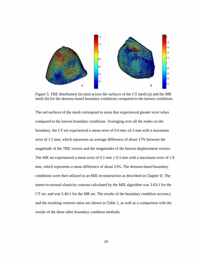
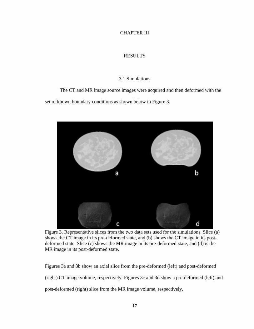
 Figure 5. TRE distribution (in mm) across the surfaces of the CT mesh (a) and the MR mesh (b) for the demons-based boundary conditions compared to the known conditions.

The red surfaces of the mesh correspond to areas that experienced greater error when

compared to the known boundary conditions. Averaging over all the nodes on the

boundary, the CT set experienced a mean error of 0.6 mm ±0.3 mm with a maximum

error of 1.5 mm, which represents an average difference of about 17% between the

magnitude of the TRE vectors and the magnitudes of the known displacement vectors.

The MR set experienced a mean error of 0.5 mm ± 0.3 mm with a maximum error of 1.9

mm, which represents a mean difference of about 23%. The demons-based boundary

conditions were then utilized in an MIE reconstruction as described in Chapter II. The

tumor-to-normal elasticity contrast calculated by the MIE algorithm was 3.63:1 for the

CT set, and was 5.46:1 for the MR set. The results of the boundary condition accuracy

and the resulting contrast ratios are shown in Table 1, as well as a comparison with the

results of the three other boundary condition methods.

19  

Table 1. Comparison of boundary condition mapping error and MIE reconstruction results between the four methods. The boundary error was calculated against known boundary conditions, and the MIE reconstructions were compared against the known contrast ratio of 6:1. Boundary Condition Mapping Error MIE Reconstruction Results CT MR CT MR

Mean TRE (max) mm Mean TRE (max) mm Elasticity Contrast Ratio

Elasticity Contrast Ratio

TPS (40 pts.)* 0.30 (2.6) * 0.033 (0.6)* 5.66** 6.26** Laplace* 0.53 (2.6)* 0.48 (2.5)* 5.02** 673** Diffusion* 1.5 (8)* 0.61 (2.9)* 17.5** 348** Demons 0.60 (1.5) 0.50 (1.9) 3.63 5.46

* (Ong, Ou et al. 2010) **(Ou, Ong et al. 2008)

Figure 6 below illustrates the relationship between elasticity contrast ratios (tumor-to-

normal) and the associated objective function values in the MIE optimization routine.

The minima in the objective function space correspond to elasticity contrast values which

resulted in an optimally deformed image. Shown in the figure are the objective function

values of the deformations using the known boundary conditions (as the control) and the

demons boundary conditions.

20  

 Figure 6. Objective function maps for the CT simulation (a) and the MR simulation (b). The objective function value calculated by the optimization framework is plotted on the ordinate axis against selected elasticity contrast ratios (tumor-to-normal) as affected by the boundary conditions. Shown are the objective maps of the demons case (solid lines) and the known boundary conditions as the control (dashed lines). The ordinate is scaled in both cases.

21  

3.2 Phantom Experiment 1

CT images of Phantom 1 were acquired at no compression, 50% compression, and

100% compression and segmented from the compression chamber. Representative slices

of the phantom at each deformation state are shown below in Figure 7.

 Figure 7. Surface renderings and representative slices from Phantom 1 at each state of deformation. This phantom exhibits little contrast and contains no tumor, and so was used only for testing boundary condition accuracy instead of a full MIE reconstruction. The figures in (a) and (b) display the phantom with no compression, (c) and (d) display the phantom under 50% compression, and (e) and (f) display the phantom under 100% compression.  

22  

The demons method was then used to generate Type I boundary conditions to map from

the uncompressed state to the 50% state, and another set of boundary conditions to map

from the uncompressed state to the 100% state. The implanted beads on the surface of the

phantom were used to calculate the TRE of this surface registration in both cases. The

average TRE for 50% compression when using the demons boundary conditions was

approximately 3.3 mm ±1.32 mm, with a maximum TRE of about 6.1 mm. The average

TRE for 100% compression was approximately 6.8 mm ±3.2 mm, which a maximum of

about 14.2 mm. The Phantom 1 results are directly compared in Table 2 (see Section 3.3)

to the gold standard TPS result and the results of the previous semi-automated methods,

as well as to analogous results from Phantom 2 and Phantom 3.

3.3 Phantom Experiment 2

CT images of Phantom 2 and Phantom 3 were acquired and segmented from the

compression chamber. The surfaces of the pre-deformed and post-deformed phantoms are

displayed in Figures 8 and 9, as well as representative slices of their respective image

volumes showing displacement of the tumor when subjected to the air bladder

compression.

23  

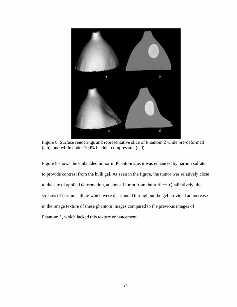
 Figure 8. Surface renderings and representative slice of Phantom 2 while pre-deformed (a,b), and while under 100% bladder compression (c,d).  

Figure 8 shows the embedded tumor in Phantom 2 as it was enhanced by barium sulfate

to provide contrast from the bulk gel. As seen in the figure, the tumor was relatively close

to the site of applied deformation, at about 12 mm from the surface. Qualitatively, the

streams of barium sulfate which were distributed throughout the gel provided an increase

in the image texture of these phantom images compared to the previous images of

Phantom 1, which lacked this texture enhancement.

24  

 Figure 9. Surface renderings and representative slice of Phantom 3 while pre-deformed (a,b), and while under 100% bladder compression (c,d).

Figure 9 shows that the images and applied deformation for Phantom 3 were similar to

those of Phantom 2. However, the tumor in this case was located further from the site of

depression than in Phantom 2, at about 26 mm from the surface.

The demons method was applied to each phantom data set to acquire Type I

boundary conditions for each mesh. The TRE of the demons-based conditions was then

evaluated by comparing to the known point correspondence of the implanted surface

beads. The average demons-based TRE for Phantom 2 was calculated to be

approximately 1.6 mm ±1.0 mm, with a maximum experienced TRE of 4.9 mm. For

Phantom 3, the average TRE was 1.9 mm ±1.2 mm, with a maximum experienced TRE

of 4.3 mm. These values are directly compared in Table 2 to the performance of the gold

standard TPS interpolation method and two previous semi-automated methods, as well as

25  

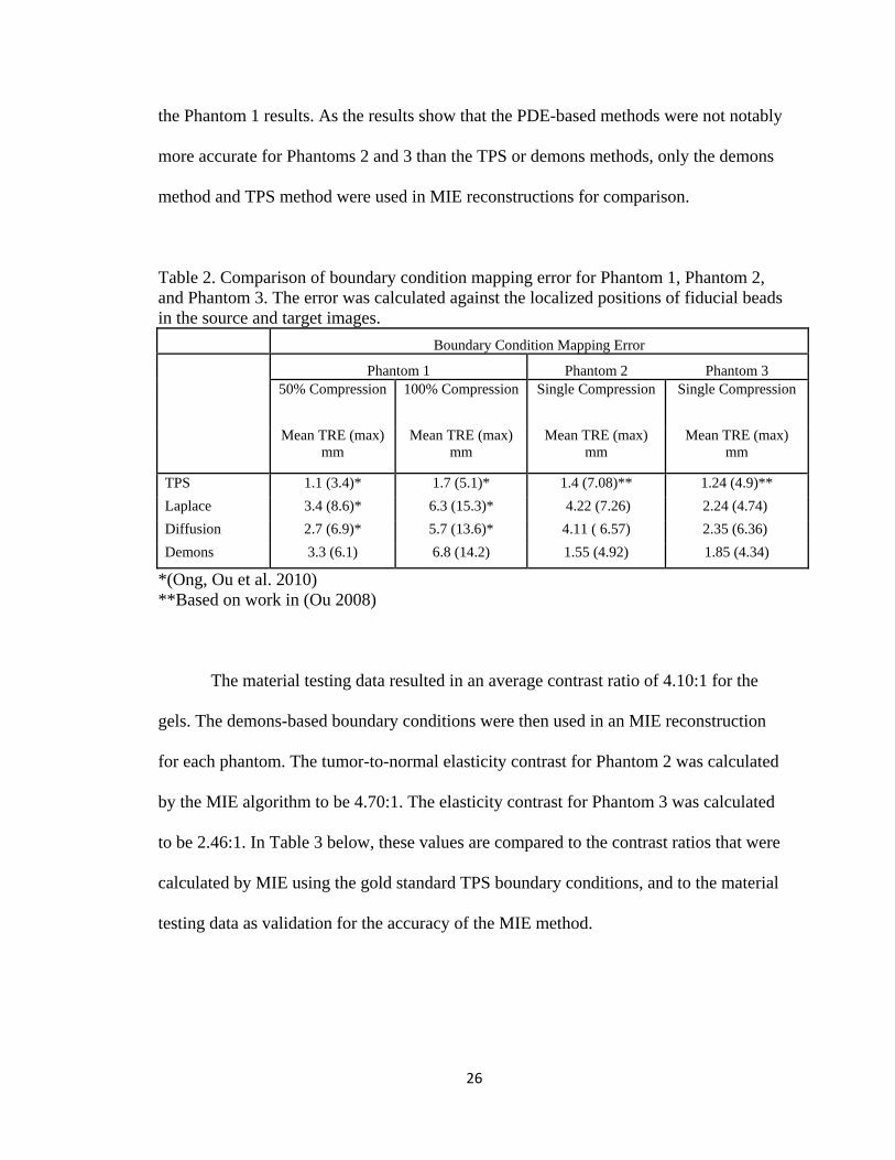
the Phantom 1 results. As the results show that the PDE-based methods were not notably

more accurate for Phantoms 2 and 3 than the TPS or demons methods, only the demons

method and TPS method were used in MIE reconstructions for comparison.

Table 2. Comparison of boundary condition mapping error for Phantom 1, Phantom 2, and Phantom 3. The error was calculated against the localized positions of fiducial beads in the source and target images. Boundary Condition Mapping Error

Phantom 1 Phantom 2 Phantom 3

50% Compression 100% Compression Single Compression Single Compression

Mean TRE (max) mm

Mean TRE (max) mm

Mean TRE (max) mm

Mean TRE (max) mm

TPS 1.1 (3.4)* 1.7 (5.1)* 1.4 (7.08)** 1.24 (4.9)** Laplace 3.4 (8.6)* 6.3 (15.3)* 4.22 (7.26) 2.24 (4.74) Diffusion 2.7 (6.9)* 5.7 (13.6)* 4.11 ( 6.57) 2.35 (6.36) Demons 3.3 (6.1) 6.8 (14.2) 1.55 (4.92) 1.85 (4.34)

*(Ong, Ou et al. 2010) **Based on work in (Ou 2008)

The material testing data resulted in an average contrast ratio of 4.10:1 for the

gels. The demons-based boundary conditions were then used in an MIE reconstruction

for each phantom. The tumor-to-normal elasticity contrast for Phantom 2 was calculated

by the MIE algorithm to be 4.70:1. The elasticity contrast for Phantom 3 was calculated

to be 2.46:1. In Table 3 below, these values are compared to the contrast ratios that were

calculated by MIE using the gold standard TPS boundary conditions, and to the material

testing data as validation for the accuracy of the MIE method.

26  

Table 3. Comparison of the MIE-reconstructed elasticity contrast ratios for Phantom 2 and Phantom 3 when using TPS and demons boundary conditions, as well as the mean contrast observed via material testing of the gels. Phantom 2

Reconstructed Contrast Ratio

Phantom 3 Reconstructed Contrast Ratio

Material Tester Contrast Ratio*

TPS* 3.81 3.06 4.10

Demons 4.70 2.46

*(Ou, Ong et al. 2008)

Figure 10 below illustrates the relationship between elasticity contrast ratios (tumor-to-

normal) and the associated objective function values in the MIE optimization routine.

Shown in the figure are the objective function values of the deformations using the TPS

boundary conditions (as the control) and the demons boundary conditions.

27  

 

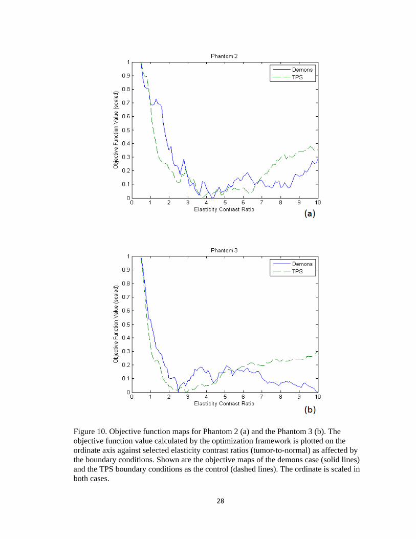
Figure 10. Objective function maps for Phantom 2 (a) and the Phantom 3 (b). The objective function value calculated by the optimization framework is plotted on the ordinate axis against selected elasticity contrast ratios (tumor-to-normal) as affected by the boundary conditions. Shown are the objective maps of the demons case (solid lines) and the TPS boundary conditions as the control (dashed lines). The ordinate is scaled in both cases.

28  

CHAPTER IV

DISCUSSION

4.1 Simulations

The demons-based boundary conditions resulted in deformed meshes which were

qualitatively very close in appearance to the known target meshes for both the CT and

MR data sets. Quantitatively, the average difference between the demons conditions and

the known conditions was about 20% for both sets, which was an encouraging indication

of the ability of the demons methods to automatically provide boundary conditions which

would have adequate accuracy for use in MIE. In Figure 5, it can be seen that the largest

errors were spread across the regions of high curvature around the tip of the breast and in

the dip of the artificial depression for the CT set, while in the MR set the errors were

mostly localized to the depression area.

The accuracy of the demons-based boundary conditions for the CT simulation

was compared to the results of past methods in Table 1 (see Section 3.1). Unsurprisingly,

the TPS method remained the most accurate of the four methods when considering the

average boundary condition error. The demons method performed about as well as the

Laplace method, and clearly outperformed the diffusion method in terms of the average

error. However, the demons method performed favorably compared to all of the other

methods in terms of maximum TRE, as its maximum error was well below those of the

other methods.

A similar comparison of these boundary condition methods applied to the MR

simulation was also shown in Table 1. The TPS interpolation again resulted in the most

29  

accurately generated boundary conditions of the four methods. In terms of average

surface TRE, the demons method was also again comparable to the Laplace method, as

well as the diffusion method in this case. However, with the exception of the TPS

method, the demons boundary conditions once again compared favorably against the

other methods in terms of the maximum error experienced on the boundary.

The results of the boundary condition accuracy experiment were encouraging and

indicated that demons-based boundary conditions were a feasible solution to the MIE

boundary condition problem. The results of the MIE reconstruction for the CT and MR

sets were shown in Table 1 and compared to the results of reconstructions which utilized

boundary conditions generated from the other three methods. Unsurprisingly, the table

shows that the TPS boundary conditions, which were the most accurate of the four,

resulted in elasticity contrast ratios for both sets that were closer to the known ratio of 6:1

than any of the other boundary conditions. For the application of the demons registration-

based boundary conditions to the CT data set, the elasticity reconstruction with spatial a

priori knowledge of the tumor successfully converged to a contrast ratio of 3.63:1.

Similarly, the MR data resulted in a contrast ratio of 5.46:1. Compared to the known

designated material contrast of 6:1, there is clearly a discrepancy in these reconstruction

behaviors that needs to be investigated. The difference, particularly between the different

modalities of input data, is likely due to a combination of factors including mesh

geometry and image quality. In addition, the distance of the tumor from the area of

greatest displacement likely affects the accuracy of the reconstruction since the

displacements of nodes are expected to decrease the further they are located away from

the depression. These simulations did not investigate the effect of tumor distance on the

30  

reconstruction. Interestingly, the diffusion method resulted in a much higher contrast

ratio for the CT set than the demons method, while the Laplace method resulted in a

contrast ratio that was closer to 6:1 but was an underestimation rather than an

overestimation of the true value. The ability of the demons-based conditions to provide a

contrast that was more accurate than the diffusion method for the CT simulation was

encouraging. Even more suggestive was the behavior of the MR reconstruction. The

Laplace and diffusion boundary conditions introduced instabilities into the MIE

algorithm, which resulted in contrast estimates that were unreasonably higher than the

true value. The demons-based conditions allowed the algorithm to provide a contrast

estimate which was closer to the known value.

It is also interesting to note the effect of the demons boundary conditions on the

optimization, as shown in Figure 6. Introducing the inexact demons boundary conditions

to the model had a noticeable effect by shifting the minimum objective function value to

a different optimal elastic contrast ratio for both the CT and the MR simulation. The shift

was much more pronounced for the CT simulation, for which the new optimal objective

function value corresponded to a contrast ratio of about 3.80:1 instead of 6:1 as predicted

by the known boundary conditions. Additionally, the convexity of the function was

altered significantly, with very little variation in the objective function for contrast ratios

in the immediate vicinity of the global minimum. The MR simulation also experienced a

shift in the optimal objective function when demons boundary conditions were used

instead of the known conditions, with a new optimal contrast of about 5.50:1. This

represented only a slight decrease from the desired 6:1 prediction. The objective function

values arise from the image similarity metric, which again suggests that the difference in

31  

objective maps between the two simulations is influenced by the image texture

characteristics. It is also clear that the addition of inaccuracies within the boundary

conditions due to the registration process alters the nature of the objective function by

injecting local minima and undesirable variations. It is evident that some sort of iterative

filtering approach may be necessary to ensure that global minima are found.

4.2 Phantom Experiment 1

While the efficacy of the automated demons method was shown by the

simulations to be comparable to the semi-automated Laplace method and somewhat

better than the diffusion method, the simulations were in several ways performed under

optimal conditions. The image volumes qualitatively had a great deal of heterogeneity

and texture on which the demons registration could act, and with which the MIE

optimization routine could use to help accurately update material property assignments.

There was also an absolute truth with which to compare, in the form of known boundary

conditions. The first phantom experiment sought to provide additional challenge to the

demons method in its ability to generate reasonably accurate boundary conditions.

The results of the demons registration were compared to the results of the three

other methods in Table 2 (see Section 3.3) for the two compression states applied to

Phantom 1. Interestingly, the table shows that the demons algorithm performed about as

well in relation to the other PDE methods as it did in the simulation experiment. What is

interesting about this is that Phantom 1 had very little image heterogeneity and would

indicate that with a lack of image intensity contrast that the demons-based registration is

at least no worse than that achieved by the PDE methods. The gold standard TPS method

32  

gave the lowest error. As seen in Table 2, the errors given by all of the methods increased

when a larger deformation was applied to Phantom 1. The demons boundary conditions

became slightly worse in relation to the other methods at the increased level of

compression, which suggests that the number of iterations used by the demons algorithm

may need to be increased to accommodate larger differences between pre- and post-

deformation images, or that the algorithm may be somewhat more sensitive to the lack of

image intensity heterogeneity.

It is also interesting to note that in moving from simulation data to “real-world”

phantom data, the errors experienced by all four of the methods increased significantly.

The Phantom 1 image data was different from the simulation data in several key respects.

For example, the target image volume of Phantom 1 represents a completely new

acquisition, whereas in the simulation work post-deformed image sets were generated

from the pre-deformed set. This discrepancy in target image acquisition introduces some

uncertainty to the determination of source-to-target correspondence. Another major

change from the simulation experiment was the markedly smaller presence of texture in

the images due to the homogeneity of the gel. More specifically, it is interesting to note

the change in TRE performance among the Phantom 1, Phantoms 2&3, and simulation

results which are listed respectively in terms of increasing image texture. Qualitatively

observing the results across Tables 1 and 2, the trend of decreasing TRE with increasing

texture for the demons-based approach can be observed.

33  

4.3 Phantom Experiment 2

It was shown in the first phantom experiment that the demons method could

produce reasonably accurate boundary conditions compared to the semi-automated

Laplace and diffusion methods. The second phantom experiment introduced another set

of real-world data, but the images from this experiment had more texture in the form of

barium sulfate as a contrast agent, which was intended to allow the demons registration to

provide more accurate boundary conditions as needed by the MIE algorithm. In addition,

the presence of the stiff tumor allowed for a test of the MIE algorithm’s ability to

distinguish elasticity contrast in a phantom while using demons-based boundary

conditions. This experiment was thus the first in which demons-based boundary

conditions were used in an MIE reconstruction for which the true boundary conditions

were not absolutely known.

The surface errors calculated from the fiducial point correspondence for the TPS,

Laplace, diffusion and demons methods were compared in Table 2 (see Section 3.3) for

Phantom 2 and Phantom 3. Unsurprisingly, the TPS method performed better with

respect to mean accuracy. Notably, the maximum error experienced by the demons

method was less than that of the TPS method, which was similar to the result of the CT

simulation study. The two PDE-based methods presented error which was similar in

scope to their Phantom 1 results. Overall, the demons method performed considerably

better on these two phantom sets than it did on Phantom 1, and notably outperformed the

Laplacian and diffusion methods. This is most likely due to the increase in image texture

which can be qualitatively observed from visual inspection of the images. Given that

34  

clinical images tend to have even more image texture and geometric heterogeneity than

found in these phantom images, further investigation into the efficacy of the demons

method seems merited.

The utilization of the demons boundary conditions in MIE reconstructions

successfully resulted in realistic tumor-to-normal modulus contrast ratios for both

phantoms. Due to the observation that the demons method resulted in boundary

conditions with comparable (and sometimes superior) accuracy to the Laplace and

diffusion methods, only the TPS and demons boundary conditions were utilized in these

reconstructions. The results for the TPS- and demons-based MIE reconstructions were

compared to each other in Table 3 (see Section 3.3) as well as to the material tester

results. As the table shows, the elasticity contrast ratios for each phantom when using

TPS boundary conditions were reconstructed to values that were within 14-40% of the

material testing data average. The reconstructions using demons boundary conditions

resulted in contrast ratios which were very similar to those of the TPS-based

reconstructions, with only a slight drop in contrast. This suggests that the demons

boundary conditions were sufficiently accurate for the MIE algorithm to provide a

reasonable estimate of the actual gel contrast.

It is also interesting to note the effect of the demons boundary conditions on the

optimization, as shown in Figure 10. Compared to the control TPS boundary conditions,

the demons conditions had a noticeable effect by shifting the minimum objective function

value to a different optimal elastic contrast ratio for both phantoms. Additionally, the

convexity of the function was altered slightly for each. Interestingly, the global minimum

of the Phantom 2 objective function was located at an approximate contrast ratio of

35  

4.20:1, which was more similar to the material testing average of 4.10:1 than the case in

which TPS boundary conditions were used. The actual contrast ratio to which the MIE

reconstruction converged was 4.70:1, which was located on the slope of a local

minimum. This behavior was most likely a result of the regularization parameters used in

the Levenberg-Marquardt optimization. In the case of Phantom 3, the global minimum

was about 2.50:1, which was the approximate value to which the algorithm converged. In

this case, the global minimum decreased slightly when using demons instead of TPS

conditions.

Observations of Figures 6 and 10 indicate the change in algorithm performance

with respect to simulation and physical data. While the nature of a simulation-to-real

transition may be responsible for the increased error in reconstruction, there are several

other likely factors involved. Over-constraint of the problem is a possible candidate with

the incorporation of the spatial prior. The MIE method works by sampling similarity

regionally, i.e. the method breaks up evaluation into many similarity zones (usually over

100) distributed spatially over the domain. The method tries to improve the similarity

among all the zones with the use of only two parameters in this case (the elasticity of the

background and tumor). This level of constraint within this type of problem can lead to

this type of oscillatory behavior. Another possible reason is the inaccuracy in boundary

condition determination due to the dramatic difference in image heterogeneity between

simulation and real data. This is supported by the change in TRE. Related to this, it is

interesting to note the difference between CT and MR reconstruction for the simulation

work associated with Figure 6 and in light of Table 1. The first observation can be made

by comparing the control objective function map across CT and MR simulation sets in

36  

Figure 6. Both simulation sets had a contrast ratio of 6:1, with the only difference being

the level of intensity heterogeneity, and potential different breast/tumor

geometries/locations. It can be observed that the CT control had a shallower minimum

which may affect the reconstruction. When adding to this observation the objective

function maps associated with the demon-based boundary condition it would seem at first

glance that the CT reconstruction may perform better due to its convexity; but when

observing how the minimum has been shifted, and in light of the shape of the control that

has no error in boundary conditions, it can be seen that in fact the MR demons-based

objective function maps more closely to its control which is reflected in the elasticity

contrast ratio.

37  

CHAPTER V

CONCLUSION

The simulations and both phantom experiments conducted in this work indicate

that while TPS interpolation remains the most accurate method used thus far in MIE for

generating boundary conditions, the demons method shows promise in situations where

fiducial point correspondence data may not be available. In addition, when transitioning

from simulation to real data, the discrepancy in performance between TPS and the

demons-based boundary condition mapping becomes less (at least in cases where image

intensity contrast within the domain is available). Furthermore, while the higher

accuracy of the TPS method is desirable, the much higher level of manual user

interaction and numerous fiducials needed for the method make clear the desire for

alternative methods of boundary condition generation. The previously studied PDE-based

methods represented steps toward automation of the boundary condition step, but still

required a moderate level of user interaction in manually designating boundary

conditions to various portions of the mesh. The demons method proposed represents a

fully automated approach.

While the results are encouraging, the challenge of predicting (prior to workflow

initiation) how well a pre-post deformation image set will fare prior to execution of the

demons registration and MIE optimization routine still remains. Since the demons

registration algorithm possesses diffusive behavior based upon intensity contours as

described by Thirion (1998), it is obvious that the images require a certain level of texture

38  

and intensity heterogeneity in order to provide these membranes a meaningful

registration. This is one of the likely causes of the varying performance of the demons

method in generating accurate boundary conditions among the experiments presented in

this work. The MIE algorithm has similar requirements in order to correctly optimize

image similarity at each update with respect to realistic material properties in the model.

Development of a feasibility metric which can predict the success of applying the MIE

algorithm to a given image set is a needed next step for the project.

In addition to a threshold criterion to evaluate the potential for a successful

reconstruction, the need to generate more realistic phantoms with controllable stiffness

properties is also necessary. The breast has a complex image signature even within CT

and the reproduction of those patterns coupled with controllable elasticity properties is

very challenging. While obstacles remain, the results presented here demonstrate the

potential of treating elastographic reconstructions using non-rigid image registration

approaches and that the possibility of full automation is also within reach.

39  

REFERENCES

ACS (2009). Cancer Facts & Figures 2009. Atlanta, American Cancer Society. Bilgen, M. (1999). "Target detectability in acoustic elastography." Ieee Transactions on

Ultrasonics Ferroelectrics and Frequency Control 46(5): 1128-1133. Burns-Cox, N., N. C. Avery, et al. (2001). "Changes in collagen metabolism in prostate

cancer: a host response that may alter progression." J Urol 166(5): 1698-701. Doyley, M. M., P. M. Meaney, et al. (2000). "Evaluation of an iterative reconstruction

method for quantitative elastography." Phys Med Biol 45(6): 1521-40. Goshtasby, A. (1988). "Registration of Images with Geometric Distortions." Ieee

Transactions on Geoscience and Remote Sensing 26(1): 60-64. Guo, Y., R. Sivaramakrishna, et al. (2006). "Breast image registration techniques: a

survey." Med Biol Eng Comput 44(1-2): 15-26. Ibanez, L., W. Schroeder, et al. (2005). The ITK Software Guide, Kitware, Inc. Keith, L. G., J. J. Oleszczuk, et al. (2002). "Are mammography and palpation sufficient

for breast cancer screening? A dissenting opinion." J Womens Health Gend Based Med 11(1): 17-25.

Krouskop, T. A., T. M. Wheeler, et al. (1998). "Elastic moduli of breast and prostate

tissues under compression." Ultrason Imaging 20(4): 260-74. Lee, H., K. L. Sodek, et al. (2007). "Phagocytosis of collagen by fibroblasts and invasive

cancer cells is mediated by MT1-MMP." Biochem Soc Trans 35(Pt 4): 704-6. Michaelson, J. S., M. Silverstein, et al. (2002). "Predicting the survival of patients with

breast carcinoma using tumor size." Cancer 95(4): 713-23. Miga, M. I. (2003). "A new approach to elastography using mutual information and finite

elements." Phys Med Biol 48(4): 467-80. Miga, M. I., M. P. Rothney, et al. (2005). "Modality independent elastography (MIE):

potential applications in dermoscopy." Med Phys 32(5): 1308-20. Muthupillai, R., D. J. Lomas, et al. (1995). "Magnetic resonance elastography by direct

visualization of propagating acoustic strain waves." Science 269(5232): 1854-7.

40  

41  

Ong, R. E., J. J. Ou, et al. (2010). "Non-rigid registration of breast surfaces using the laplace and diffusion equations." Biomed Eng Online 9(1): 8.

Ophir, J., I. Cespedes, et al. (1991). "Elastography: a quantitative method for imaging the

elasticity of biological tissues." Ultrason Imaging 13(2): 111-34. Ou, J. J. (2008). Development of modality-independent elastography as a method of

breast cancer detection: xiv, 169 p. (1 file). Ou, J. J., R. E. Ong, et al. (2008). "Evaluation of 3D modality-independent elastography

for breast imaging: a simulation study." Phys Med Biol 53(1): 147-63. Papademetris, X., A. J. Sinusas, et al. (2002). "Estimation of 3-D left ventricular

deformation from medical images using biomechanical models." IEEE Trans Med Imaging 21(7): 786-800.

Sullivan, J. M., G. Charron, et al. (1997). "A three-dimensional mesh generator for

arbitrary multiple material domains." Finite Elements in Analysis and Design 25(3-4): 219-241.

Thirion, J. P. (1998). "Image matching as a diffusion process: an analogy with Maxwell's

demons." Med Image Anal 2(3): 243-60. Warwick, J., L. Tabar, et al. (2004). "Time-dependent effects on survival in breast

carcinoma: results of 20 years of follow-up from the Swedish Two-County Study." Cancer 100(7): 1331-6.

Yoo, T. S., M. J. Ackerman, et al. (2002). "Engineering and algorithm design for an

image processing Api: a technical report on ITK--the Insight Toolkit." Stud Health Technol Inform 85: 586-92.