Automatic Kronecker Product Model Based Detection of Repeated Patterns in2D Urban Images∗

Juan LiuGraduate Center, CUNY

New York, NYlangelfly@hotmail.com

Emmanouil PsarakisUniversity of Patras

Patras, Greecepsarakis@ceid.upatras.gr

Ioannis StamosHunter Coll. & Grad. Center, CUNY

New York, NYistamos@hunter.cuny.edu

Abstract

Repeated patterns (such as windows, tiles, balconiesand doors) are prominent and significant features in urbanscenes. Therefore, detection of these repeated patterns be-comes very important for city scene analysis. This paperattacks the problem of repeated patterns detection in a pre-cise, efficient and automatic way, by combining traditionalfeature extraction followed by a Kronecker product low-rank modeling approach. Our method is tailored for 2D im-ages of building facades. We have developed algorithms forautomatic selection of a representative texture within facadeimages using vanishing points and Harris corners. Afterrectifying the input images, we describe novel algorithmsthat extract repeated patterns by using Kronecker productbased modeling that is based on a solid theoretical founda-tion. Our approach is unique and has not ever been used forfacade analysis. We have tested our algorithms in a largeset of images.

1. IntroductionUrban scenes contain rich periodic or near-periodic

structures, such as windows, doors, and other architectural

features. Detection of the periodic structures is useful in

many applications such as photorealistic 3D reconstruction,

2D-to-3D alignment, facade parsing, city modeling, classi-

fication, navigation, visualization in 3D map environments,

shape completion, cinematography and 3D games, just to

name a few. However it is a challenging task due to scene

occlusion, varying illumination, pose variation and sensor

noise.

The first step of all facade parsing algorithms (see [15]

for an example) is the detection and rectification of individ-

ual facade structures. The first part of our pipeline (Sec.

3) adopts vanishing points detection to compute an initial

transform matrix for rectification and for the automatic se-

∗This work has been supported in part by NSF grants IIS-0915971 and

CCF-0916452. We are grateful to the anonymous reviewers.

lection of a representative texture. The second part of our

pipeline (Secs. 4,5), after rectification, is the detection of re-

peated patterns. Current state-of-the-art methods use classi-

fication [15] or statistical approaches [13]. We, on the other

hand, provide a novel detection method that models repeti-

tion as a Kronecker product.

2. Related WorkIn recent years, repeated patterns or periodic structures

detection has received significant attention in both 2D im-

ages [17, 13] and 3D point clouds [3, 12]. Repeated patterns

are usually hypothesized from the matching of local image

features. They can be modeled as a set of sparse repeated

features [11] in which the crystallographic group theory [8]

was employed. The work of [14] maximizes local symme-

tries and separates different repetition groups via evaluation

of the local repetition quality conditionally for different rep-

etition intervals.

The work of [10] proposes an approach to detect sym-

metric structures in a rectified fronto-facade and to recon-

struct a 3D geometric model. The work of [15] describes

a method for periodic structure detection upon the pixel-

classification results of a rectified facade. Shape grammars

have also been used for 2D facade parsing [13]. Other sim-

ilar grammar-based approaches include [1].

All the above-mentioned methods require as pre-

processing image rectification. To solve this problem, low-

rank methods were used and attracted a lot of attention in

recent years [16]. A similar work was proposed by [4] in

which the rank value N is assumed known. Another method

for the recovery of both low-rank and the sparse compo-

nents is presented in [2]. Finally, [7] describes a low-rank

based method that detects the repeated patterns in 2D im-

ages for the application of shape completion.

The contributions of this paper with respect to ear-

lier work are: (a) an automated method based on vanish-

ing points for detection of representative texture within a

facade, and (b) a novel algorithm based on Kronecker prod-

uct for detection of repeated patterns within that texture of

2013 IEEE International Conference on Computer Vision

1550-5499/13 $31.00 © 2013 IEEE

DOI 10.1109/ICCV.2013.57

401

the facade image.

3. Texture Selection and RectificationThe input of this step is a 2D image of a building facade.

The output is a representative texture on the facade as well

as a transform matrix that is used to initialize the facade

rectification. This representative texture is essential for an

automated system, since it is used as input by the low-rank

algorithm (named TILT) in [16] (this automation provides

a performance improvement of 19.6% over manual selec-

tion; see the comparison in Table 1). This algorithm is im-

plemented in three steps: (1) feature extraction, (2) block

division, and (3) transform initialization and representative

texture selection.

First of all, we extract Harris corners [5]. We also de-

tect the two major vanishing points by using the method of

[6]. We then divide the facade into blocks (quadrilateral)

along vanishing points directions. Finally, we compute the

homography matrix that rectifies the image and select the

representative texture by combining Harris corners distri-

bution information within the detected blocks. We observed

that Harris corners are distributed almost uniformly in un-

occluded facade areas that contain repeated patterns. Oth-

erwise occlusions may produce a non-uniform distribution

of the Harris corners. For example, the Harris corners in a

tree area will be very dense and non-uniformly spaced.

In particular, starting from each detected vanishing point

we draw hypothetical lines at angular intervals towards the

image assuring that all Harris corners are included in the

generated quadrilaterals (see Fig. 1(a)). This is achieved

by computing the smallest angles θ1 and θ2 (one for each

vanishing point) that ensure inclusion of all Harris corners.

Then, we divide each range θi into m parts. The intersec-

tions of the imaginary lines thus create m×m quadrilater-

als.

We observed that the number of corners in each block

does not change much after perspective distortion of the

facade image, although the distribution of the Harris corners

depends on the location of the vanishing points. Excluding

strong perspective distortions is not so crucial (in such cases

even robust techniques fail to rectify the image). We thus

assume that the ideal texture should consist of neighboring

blocks that have a similar and uniform distribution of Har-

ris corners. We then count the number of Harris corners in

each block, and get an m × m matrix C, where each ele-

ment Ci, j , i, j = 1, · · · ,m is the number of Harris corners

in the corresponding block.

In order to isolate the r × c submatrix of C1 containing

the most representative texture of the given facade, let us

consider that its elements are random samples from a dou-

ble exponential distribution. We then compute the sample

1In all of our experiments, we set m to 10 and fix r and c to a given

percentage of m, that is r = c = 0.4m.

(a) (b) (c) (d)Figure 1. (a) 10 by 10 blocks divided along detected vanishing

points directions. (b) Yellow quadrilateral shows r× c blocks that

compose the representative texture. (c) Red box, defined by the

largest rectangle within the representative texture, is the input to

the TILT algorithm. In green is the yellow quadrilateral from (c).

(d) Rectified facade by TILT, with automatically selected texture

shown inside the pink box.

median μC of the elements of matrix C. Finally, we slide

a window of size r × c along matrix C, and compute in

each location the sample mean deviation from the sample

median, that is:

Si,j =1

rc

i+r−1∑k=i

j+c−1∑l=j

|Ck, l − μC| (1)

thus forming a score matrix of size (m−r+1)× (m−c+1).It is well known that the sample median and the sample

mean deviation from the sample median are the maximum

likelihood estimators of the mean and standard deviation of

the distribution. Thus, by choosing the sliding window with

the highest score we actually choose the one with the min-

imum variance among all the best likelihood estimators of

the mean value. This window will be selected and used as

the input of the TILT algorithm in order to get the low-rank

component and rectification of the facade image (see Fig.

1 for an example). Note that this low-rank component is

not used by our algorithms, since we have a novel way of

calculating it (see Sec. 4).

4. Facade Modeling via Kronecker ProductsIn this section we describe our Kronecker product mod-

eling approach that is applied on a rectified facade image.

It is a novel representation that describes a large subset of

facade examples.

4.1. Ideal Facade Modeling

To this end, let us consider the partition of all ones or-

thogonal array 1lv×lh of size lv× lh by using the following

mutually exclusive, 1−0 2 matrices Mk, k = 1, 2, · · · , Kof size lv × lh each, that is:

< vec{Mk}, vec{Ml} > =

{||vec{Mk}||0, k = l

0, k �= l(2)

K∑k=1

Mk = 1lv×lh (3)

2Matrices that contain only combinations of 1s and 0s

402

where vec{X}, < x, y > and ||x||0 denote the column-wise vectorization of matrix X, the inner product of vectors

x, y and the l0 norm of vector x respectively. As it is clear

from Eqs. (2-3), different choices of matrices Mk result in

different partitions of orthogonal block 1lv×lh .

Let us now associate with each component Mk, k =1, 2, · · · , K of the partition of array 1lv×lh defined in

Eq. (3), a 2-D pattern Pk of size Nv × Nh that is going to

be repeated according to Mk. The patterns should have a

piecewise constant surface form. In particular, with the aim

of patterns Pk several windows, doors and/or balconies of

different architectures can be formed.

We can now define a subset of urban building facades

that can be expressed as a sum of Kronecker products:

FN×M =

K∑k=1

λk(Mk ⊗Pk) (4)

where X ⊗Y is the Kronecker product of matrices X, Yand λk, k1 = 1, 2, · · · ,K are weights. Finally, N ×M is

the size of the urban building facade image. By the defini-

tion of the Kronecker product it is obvious that N = lvNv

and M = lhNh. Please note that the urban building

facade’s model defined in Eq. (4) can be used even in cases

where there is not any periodic structure in the given input

facade we would like to model.

Generalizing Eq. (4) to permit a “wall” gray level λ0, we

get:

FN×M = λ01N1tM +

K∑k=1

λk(Mk ⊗Pk). (5)

Using the fact that the components of the partition of or-

thogonal array 1lv×lh of Eq. (3) are mutually exclusive, we

rewrite Eq. (5) as:

FN×M =

K∑k=1

λk(Mk⊗Pk), Pk = Pk+λ0

λk1Nv1

tNh

(6)

where Pk are modified patterns as defined above, and

1Nv , 1Nhare all ones vectors with the subscripts denoting

their lengths.

4.2. Ideal Facade Model Approximation

In this section we would like to compute (or approxi-

mate) the components of the Kronecker product that gener-

ate a given ideal (i.e. noise-free) building facade FN×M ∈R

N×M with N = lvNv and M = lhNh. Using the model

defined in Eq. (6) we can define the following cost function:

CF(Mk , Pk, λk, k = 1, · · · ,K) = ||FN×M −FN×M ||22

= ||FN×M −K∑

k=1

λk(Mk ⊗ Pk)||22, (7)

where Mk, Pk and λk, k = 1, 2, · · · ,K denote the par-

tition matrices, the patterns and the weighting factors of

facade’s model respectively. As it is clear from its defini-

tion CF(.) is a Frobenious norm based cost function that

quantifies the error between the given matrix FN×M and

the model FN×M .

Therefore, the modeling problem of the given urban

building facade FN×M can be expressed by the following

minimization problem

minMk,Pk,λk, k=1,··· ,K

CF (Mk, Pk, λk, k = 1, · · · ,K),

(8)

which is known as the Nearest Kronecker Product problem

[9]. The following partition of the given matrix FN×M is

key for the solution of the above problem:

FN×M =

⎡⎢⎢⎢⎣

F11 F12 · · · F1lh

F21 F22 · · · F2lh...

.... . .

...

Flv1 Flv2 · · · Flvlh

⎤⎥⎥⎥⎦ , (9)

where Fij is a block of size Nv × Nh. We can then form

the matrix

Flvlh×NvNh=[vec{F11} vec{F21} . . . vec{Flvlh}

]T(10)

which constitutes a rearrangement of the given facade ma-

trix FN×M . Using the above defined quantities, the cost

function of Eq. (7) can be equivalently expressed as:

CF(mk, pk,λk, k = 1, · · · ,K)

= ||Flvlh×NvNh−

K∑k=1

λkmkptk||22 (11)

where mk, pk are the column-wise vectorized forms of ma-

trices Mk, Pk. By exploiting the above defined equivalent

form of the cost function, the Kronecker Product SV D[9] can be used to solve the optimization problem of Eq. (8):

Theorem 1: Let Flvlh×NvNh= VΣUT be the Singular

Value Decomposition of the rearranged counterpart of ma-

trix FN×M . Let us also consider the following diagonal

matrix

ΣK = diag {σ1 σ2 · · · σK} (12)

containing the first K singular values of matrix

Flvlh×NvNh, and let

VK = [v1 v2 · · ·vK ], UK = [u1 u2 · · ·uK ] (13)

be the K associated left and right singular vectors respec-

tively. Then, the matrices M�k, the patterns P�

k, and the

weighting factors λ�k that satisfy:

vec{M�k} = vk, vec{P�

k} = uk, λ�k = σk, k = 1, 2, · · · ,K

(14)

403

constitute the optimal solution of the optimization problem

of Eq. (8).

Using Theorem 1, we can find an optimal approxima-

tion that has the desired form, i.e. it is a sum of Kronecker

products, that minimizes the cost function defined in Eq.

(7). Note, however, that some of the characteristics of the

optimal solution, are not consistent with the ingredients of

the facade model defined in (5) thus making the direct use

of Theorem 1 problematic. Specifically, neither the opti-

mal matrices M�k neither the optimal patterns P�

k have, in

the general case, the desired form, that is they are not 1-0

matrices and piecewise constant surfaces, respectively. In

addition, the vectorized form of the optimal patterns are or-

thonormal to each other.In order to impose one of the requirements of the pro-

posed facade model, in the sequel we consider that matrices

Mk have the desired 1 − 0 form and are known. In such a

case, we form the cost function:

CF(Pk, λk, k = 1, · · · ,K|Mk), (15)

which is the cost function of Eq. (8) but with the partition

matrices known. We would like to minimize it with respect

to the patterns Pk and the weighting factors λk. The solu-

tion of the new optimization problem is the subject of the

next lemma.

Lemma 1: Assuming that the matrices Mk, k =1, 2, · · · ,K defined in Eqs. (2-3) are known, then the min-

imization of the cost function defined in Eq. (15) produces

patterns Pk and weighting factors λk that are related as fol-

lows:

λ�kvec{P�

k}=UΣTVT vec{Mk}||vec{Mk}||22

, k = 1, 2, · · · ,K(16)

Proof: Using the fact that ||F||22 = trace{FTF}, the

SVD decomposition of the rearranged counterpart of ma-

trix FN×M , the linearity of the trace operator, and after

some simple mathematical manipulations, the cost function

defined in Eq. (11) can be rewritten as follows:

CF( Pk, λk, k = 1, · · · ,K|Mk) = trace{UΣTΣUT

}−trace

{UΣTVT

K∑k=1

λkmkptk+

K∑k=1

λkpkmtkVΣUT

}+

trace

{(K∑

k=1

λkmkptk

)(K∑

k=1

λkpkmtk

)}.

Moreover, using the orthogonality of vectors mk, k =1, 2, · · · ,K, the orthonormality of matrix U, the commu-

tative property of trace operator, and by interchanging the

order of summations and trace operator, we obtain:

CF( Pk, λk, k = 1, · · · ,K |Mk) = trace{ΣTΣ

}−2

K∑k=1

λktrace{ptkUΣTVTmk

}+

K∑k=1

λ2k||mk||22||pk||22.

50 100 150 200 250 300 350 400 450 500 550

50

100

150

200

250

50 100 150 200 250 300 350 400 450 500 550

50

100

150

200

250

50 100 150 200 250 300 350 400 450 500 550

50

100

150

200

250

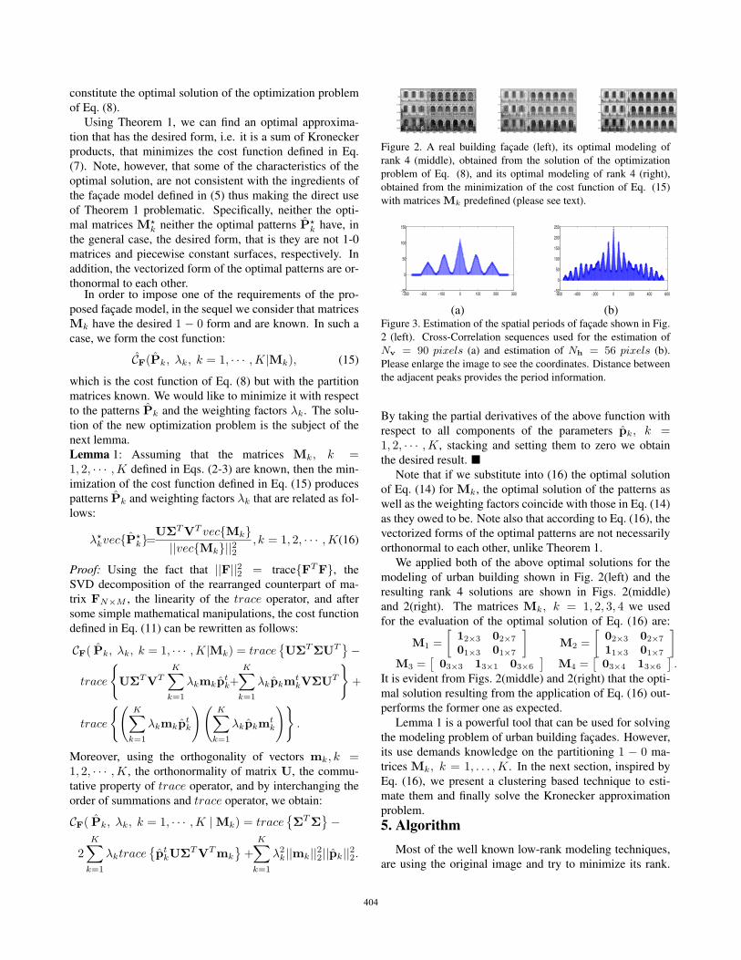
Figure 2. A real building facade (left), its optimal modeling of

rank 4 (middle), obtained from the solution of the optimization

problem of Eq. (8), and its optimal modeling of rank 4 (right),

obtained from the minimization of the cost function of Eq. (15)

with matrices Mk predefined (please see text).

−300 −200 −100 0 100 200 300−50

0

50

100

150

−600 −400 −200 0 200 400 600−50

0

50

100

150

200

250

(a) (b)Figure 3. Estimation of the spatial periods of facade shown in Fig.

2 (left). Cross-Correlation sequences used for the estimation of

Nv = 90 pixels (a) and estimation of Nh = 56 pixels (b).

Please enlarge the image to see the coordinates. Distance between

the adjacent peaks provides the period information.

By taking the partial derivatives of the above function with

respect to all components of the parameters pk, k =1, 2, · · · ,K, stacking and setting them to zero we obtain

the desired result. �Note that if we substitute into (16) the optimal solution

of Eq. (14) for Mk, the optimal solution of the patterns as

well as the weighting factors coincide with those in Eq. (14)

as they owed to be. Note also that according to Eq. (16), the

vectorized forms of the optimal patterns are not necessarily

orthonormal to each other, unlike Theorem 1.

We applied both of the above optimal solutions for the

modeling of urban building shown in Fig. 2(left) and the

resulting rank 4 solutions are shown in Figs. 2(middle)

and 2(right). The matrices Mk, k = 1, 2, 3, 4 we used

for the evaluation of the optimal solution of Eq. (16) are:

M1 =

[12×3 02×7

01×3 01×7

]M2 =

[02×3 02×7

11×3 01×7

]M3 =

[03×3 13×1 03×6

]M4 =

[03×4 13×6

].

It is evident from Figs. 2(middle) and 2(right) that the opti-

mal solution resulting from the application of Eq. (16) out-

performs the former one as expected.

Lemma 1 is a powerful tool that can be used for solving

the modeling problem of urban building facades. However,

its use demands knowledge on the partitioning 1 − 0 ma-

trices Mk, k = 1, . . . ,K. In the next section, inspired by

Eq. (16), we present a clustering based technique to esti-

mate them and finally solve the Kronecker approximation

problem.

5. AlgorithmMost of the well known low-rank modeling techniques,

are using the original image and try to minimize its rank.

404

We, on the other hand, use a Kronecker product based

model FN×M . We are thus able to express the cost func-

tion defined in Eq. (7) in an equivalent form (11). This is

essential, since by transforming the given matrix FN×M

into its rearranged counterpart Flvlh×NvNh, we form a ma-

trix whose rank is drastically reduced (it is upper bounded

by the smallest dimension of the above mentioned matrix,

which usually is equal to lvlh). Our algorithm starts with

the estimation of the size Nv×Nh of the patterns (Sec. 5.4),

continues with the estimation of K and the actual partition

matrices (Secs. 5.1-5.2) and concludes with the computa-

tion of pattern matrices and weights (Sec. 5.3).

5.1. Estimating K by Clustering

Here we assume that we know the parameters Nv and

Nh (we will show how to compute them in Sec. 5.4). We

will describe an iterative technique which is based on the

idea of clustering the rows of the rearranged counterpart of

the given matrix FN×M . In particular, we use a partitional(k-means) clustering algorithm in an iterative fashion in or-

der to accurately estimate the rank of that matrix.

To this end, let us consider that matrix Flvlh×NvNh(for

simplicity in the notation from now on we will denote it by

F), as well as the desired number of clusters we would like

to group the rows of the matrix (let us denote it by K) be

given, and let us define the following set consisting of Kgroups:

Rk = {f tq : ||f tq − rtk||22 ≤ ||f tq − rtl ||22, ∀ 1 ≤ l ≤ K}k = 1, 2, · · · ,K (17)

where f tq denotes the q-th row of matrix F, and rtk the mean

of the k-th group of the rows respectively, as computed by

k-means.

Let us also define the corresponding indicator vectors

of length lvlh each:

1Rk[q] =

{1 if f tq ∈ Rk

0 otherwise, q = {1, 2, · · · , lvlh}(18)

and the element-wise mean vectors of each group:

rtk = mean{Rk}, k = 1, 2, · · · , K (19)

We can now define the following matrix:

FR =K∑

k=1

1Rkrtk (20)

which has the same size as F. More importantly, if the given

number of clusters K were the correct one, then K should

equal to the rank of F. If, on the other hand, the given

number of clusters K is greater than the real rank of F, then

the rank of FR will be smaller than K. Hence, by defining

the new number of the clusters as:

K = rank(FR) (21)

and repeating the above described procedure, we are ex-

pecting that after some iterations, FR will be the desired

approximation of F. Note that the computation of rank in

Eq. (21) and as part of Algorithm 1, is a generic algorithm

and not one that minimizes the rank of a matrix.

Algorithm 1: Kronecker Facade Modeling, noise-free ideal

case. Input: F, K = rank(F)

1: repeat2: Form groupsRk, k = 1, . . . ,K via k-means (17)

3: Form the indicator vectors 1Rkof (18)

4: Form the mean vectors rtk

of (19)

5: Compute the matrix FR defined in (20)

6: Compute its rank K (21)

7: Assign FR to F8: until convergence

9: Output: F�R, K

�, 1Rk.

Note that rtk, k = 1, 2, · · · ,K� are the rows of F�

R.

Note also that the use of mean in Eq. (19) is in exact ac-

cordance with Lemma 1 (as will be seen in Sec. 5.3). This

will provide the optimal result assuming an ideal noise-free

case.

In practice though, due to variations caused by occlu-

sions (such as trees, traffic lights, etc.), shadows, etc., in-

stead of the mean in Step 4, we use the element-wise

median operator:rtk = median{Rk}. (22)

This is based on the robustness of the median operator (used

for the estimation of the most characteristic values of rows

that belong to the same cluster) and its optimality in the L1

sense.

A second modification is also essential. Unfortunately,

Lemma 1 does not guarantee that the patterns are piece-wise

constant. One way to enforce that constraint is by also forc-

ing clustering in the columns of F as well (note that each

column spans all patterns). We thus consider the matrix:

G =1

2(FC + FR) (23)

and the new number of the clusters:

K = min{rank(FR), rank(FC)}, (24)

where FC is the column-wise clustering result. It is obtained

by following the same k-means clustering, but now in the

columns:

Ck = {fp : ||fp − ck||22 ≤ ||fp − cl||22, ∀ 1 ≤ l ≤ K}k = 1, 2, · · · ,K (25)

where fp denotes the p-th column of matrix F, and ckdenotes the mean of the k-th group of the columns re-

spectively. The corresponding indicator vectors of length

405

NvNh is defined as:

1Ck [p] =

{1, if fp ∈ Ck0 otherwise, p = {1, 2, · · · , NvNh}

(26)

and the element-wise median vectors of each group:

ck = median{Ck}, k = 1, 2, · · · , K. (27)

Then,

FC =K∑

k=1

ck1tCk . (28)

Therefore, the algorithm we use in practice is shown below.

Algorithm 2: Kronecker Facade Modeling. Input: F, K =rank(F)

1: repeat2: Form groups Rk, Ck k = 1, . . . ,K via k-means

(17),(25)

3: Form the indicator vectors 1Rk, 1Ck of (18), (26)

4: Form the vectors rtk, ck of (22), (27)

5: Form the matrices FR, FC and G of (20), (28) and

(23)

6: Set K using (24)

7: Assign G to F8: until convergence

9: Output: F�R, K

�, 1Rk.

Note that rtk, k = 1, 2, · · · ,K� are the rows of F�

R.

For the convergence condition in Algorithm 2, we can con-

sider the convergence of the sum of all entries in |Gi −Gi−1|, where Gi denotes the G obtained in the ith iter-

ation, or set the number of iterations to a maximum pre-

specified number. Finally, the denoising of matrix F after

Step 7 in the algorithm above, can drastically speed up the

convergence.

5.2. Estimating Matrices Mk, k = 1, 2, · · · ,K�

We estimate matrices Mk, k = 1, 2, · · · ,K� by reshap-

ing each one of the K� above mentioned indicator vectors

into their nominal form, that is, in a rectangular array of size

lh × lv each.

Algorithm 3: Estimation of Matrices Mk. Input: 1Rk,K�

1: for k = 1 to K� do2: mk = 1Rk

3: Mk = reshape(mk, lh, lv)4: end for5: Output: Mk, k = 1, . . . , K�.

We must stress at this point that it is easy to validate

that the vectorized forms of the estimated partition matrices

satisfy the conditions of Eqs. (2) and (3).

5.3. Computing Patterns and Weighting Factors

At this point we have estimated all the quantities needed

to find out the optimal patterns Pk and weighting factors

λk, k = 1, 2, · · · ,K�, as they are defined in Lemma1.

Note that the estimated partition matrices have the desired

optimal 1 − 0 form. In addition, since each mk coincides

with the corresponding indicator vector, and by the def-

inition of mean vectors r�k defined in (19), each term of

the matrix FR of (20), has exactly the same form with the

optimal patterns defined in Lemma 1. Indeed, by taking

into account that by definition mk = vec{Mk}, and be-

cause of the special 1 − 0 form of the partition matrices

||mk||22 = ||mk||0, the following is true:

λ�kvec{P�

k} =UΣTVT vec{Mk}||vec{Mk}||22

= r�k, k = 1, ...,K�.

(29)

Therefore, the vectors r�k, computed in Algorithm 1, pro-

vide us the weighted optimal patterns. In practice, as dis-

cussed in Sec. 5.1, we are using the results of Algorithm

2.

5.4. Estimating the Spatial Periods of the Patterns

In all the steps of the proposed algorithm we have as-

sumed that the spatial periods of the patterns were known.

However, they are unknown and must be estimated. Al-

though well known methods ([3, 12]) can be used for that

purpose, we propose the use of the algorithm in Sec. 5.1.

The only difference is that the input to the algorithm is the

actual facade matrix F and not its rearranged form F. In

particular, let us run Algorithm 2 for a predefined value K0

of the parameter K once with input F, and then with input

Ft. Then, we can compute the following:

||1Rk� ||0 = maxk=1,2,··· ,K0

{||1Rk||0} (30)

||1Cl� ||0 = maxl=1,2,··· ,K0

{||1Cl ||0} , (31)

and the corresponding auto-correlation sequences:

rRk� = 1R�k∗ 1R�

k(32)

cCk� = 1C�l∗ 1C�

l(33)

where ” ∗ ” denotes the correlation operator. Note that by

taking into account Eqs. (30-31), indicator vectors 1Rk� ,

1Cl� are the vectors that define the dominant row and col-

umn spatial periods respectively and thus the computa-

tion of the corresponding auto correlation sequences makes

sense. Note also that the vectors involved in the computa-

tion of the proposed auto-correlation sequences are based

on indicator vectors, that is 1−0 vectors, and not on gray-

value quantities.

406

Algorithm 4 : Estimation of Periods Nh, Nv.

Input: FN×M , K0

1: Form the vectors 1Rk, k = 1, 2, ...,K0 using (18)

2: Form the vectors 1Cl , l = 1, 2, ...,K0

3: Compute the quantities defined in Eqs. (30-31)

4: Compute the sequences defined in Eqs. (32-33)

5: Use them to estimate the desired spatial periods

6: Output: Nh and Nv.

The results we obtained with K0 = 5 in the urban build-

ing facade of Fig. 2 (left), are shown in Figs. 3 (a) and 3(b)

respectively.

6. Experiments and DiscussionThe experiments are implemented in Matlab, and run

on a computer with an 1.8 GHz Intel Core i7 CPU and a

4GB memory. To evaluate the performance of our VPD

initialization scheme (Sec. 3), we run TILT with its origi-

nal branching initialization scheme and with our vanishing

points initialization. The results are shown in Table 1. The

urban images we use for test include 182 facade images we

collected in New York City as well as 124 sample facades

from TILT’s web resources. The results clearly state that

in urban environments the use of vanishing points signifi-

cantly improve the quality of the results. We thus propose

to use our automated initialization technique in those cases

in order to first rectify and then use TILT (or other similar

methods) for improvement.

In a separate experiment we tested our repeated pattern

detection in 89 images for which we had ground-truth [13,

15]. Out of the 89 images we tested, only 4% resulted to

failure detections (see failure cases in Fig. 6). The results

from the remaining 96% were very similar to the ground-

truth. We overlaid our results with the ground-truth pixel

by pixel and had exact matches for 91% of the pixels.

A more extensive collection of results can be found in

supplemental material. In this paper we present some repre-

sentative images. Our low-rank method (Secs. 5.1, 5.2) en-

ables us to remove occlusions, small illumination variations

and photometric distortions as seen in the fourth column of

Fig. 4, 5, and 6. Because of this we have very accurate de-

tection of repeated patterns. Based on those clean patterns,

we can easily obtain 1-0 patterns (i.e. refining the results)

by applying classification methods, such as the rank-one al-

gorithm [15], within each group. Examples of detected 1-0

patterns are shown in the last column of Fig. 4, 5, and 6. For

example the method of [15] fails in the case of Fig. 5, due

to tree occlusion. Our algorithm, however, can successfully

detect four different clusters and clear pattern structures.

We can conclude that the block partition Sec. 5.4 is not

a bottleneck of our algorithm. The partition lines may pass

across the desired patterns, as shown in the second row of

Fig.6. In such cases some pattern is divided into two ad-

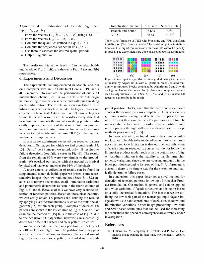
Initialization method Run Time Success Rate

Branch-and-bound 36.63s 65%VPD 38.6s 84.6%

Table 1. Performance of TILT with branching and VPD transform

initialization (Sec. 3) respectively. The vanishing points initializa-

tion results in significant increase in success rate without a penalty

in speed. The experiments are done on a set of 306 facade images.

(a) (b) (c) (d) (e)Figure 4. (a) Input image, (b) partition grid showing the periods

estimated by Algorithm 4, with all partition blocks colored ran-

domly, (c) grouped blocks generated by Algorithms 2 and 3, with

each group having the same color, (d) low-rank component gener-

ated by Algorithms 2 - 4 in Sec. 5.1 - 5.4, and (e) estimated 1-0

repeated patterns by refining (d).

jacent partition blocks, such that the partition blocks don’t

contain the desired patterns completely. However our al-

gorithm is robust enough to detected them separately. We

must stress at this point that a better partition can definitely

improve the performance. In order to have partition lines

mostly passing through wall areas as desired, we can adopt

methods proposed in [10, 3].

In the experiments, we found most of the common build-

ing facades to be able to be modeled by our Kronecker prod-

uct structure. One limitation is that our method fails when

a facade contains repeated structures that do not follow the

Kronecker product model, such as in the bottom row of Fig.

6. Another limitation is the inability to handle large pho-

tometric variations, since they are causing ambiguity in the

block partition (second to last row of Fig. 6). Unfortunately,

currently there is no simple way for the system to automat-

ically determine failure cases.

In conclusion, this paper describes a novel method for

detection of repeated patterns following a Kronecker Prod-

uct formulation. Our method is general and can be applied

to a wide variation of facade structures and is being based

on a solid theoretical foundation. The fact that we are uti-

lizing the low-rank part of the rearranged input facade im-

age allows us to handle problems of occlusion, shadows and

illumination variations. Other image processing, low-rank

and SVD-based techniques that can be used for increasing

the robustness and speed of convergence are currently under

investigation.

References[1] O. Barinova, V. Lempitsky, E. Tretiak, and P. Kohli. Ge-

ometric image parsing in man-made environments. ECCV,

2010.

407

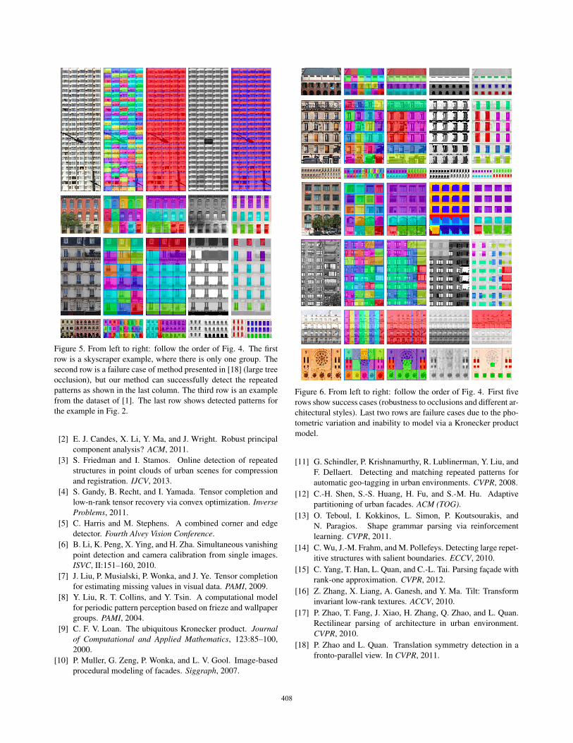
Figure 5. From left to right: follow the order of Fig. 4. The first

row is a skyscraper example, where there is only one group. The

second row is a failure case of method presented in [18] (large tree

occlusion), but our method can successfully detect the repeated

patterns as shown in the last column. The third row is an example

from the dataset of [1]. The last row shows detected patterns for

the example in Fig. 2.

[2] E. J. Candes, X. Li, Y. Ma, and J. Wright. Robust principal

component analysis? ACM, 2011.

[3] S. Friedman and I. Stamos. Online detection of repeated

structures in point clouds of urban scenes for compression

and registration. IJCV, 2013.

[4] S. Gandy, B. Recht, and I. Yamada. Tensor completion and

low-n-rank tensor recovery via convex optimization. InverseProblems, 2011.

[5] C. Harris and M. Stephens. A combined corner and edge

detector. Fourth Alvey Vision Conference.

[6] B. Li, K. Peng, X. Ying, and H. Zha. Simultaneous vanishing

point detection and camera calibration from single images.

ISVC, II:151–160, 2010.

[7] J. Liu, P. Musialski, P. Wonka, and J. Ye. Tensor completion

for estimating missing values in visual data. PAMI, 2009.

[8] Y. Liu, R. T. Collins, and Y. Tsin. A computational model

for periodic pattern perception based on frieze and wallpaper

groups. PAMI, 2004.

[9] C. F. V. Loan. The ubiquitous Kronecker product. Journalof Computational and Applied Mathematics, 123:85–100,

2000.

[10] P. Muller, G. Zeng, P. Wonka, and L. V. Gool. Image-based

procedural modeling of facades. Siggraph, 2007.

Figure 6. From left to right: follow the order of Fig. 4. First five

rows show success cases (robustness to occlusions and different ar-

chitectural styles). Last two rows are failure cases due to the pho-

tometric variation and inability to model via a Kronecker product

model.

[11] G. Schindler, P. Krishnamurthy, R. Lublinerman, Y. Liu, and

F. Dellaert. Detecting and matching repeated patterns for

automatic geo-tagging in urban environments. CVPR, 2008.

[12] C.-H. Shen, S.-S. Huang, H. Fu, and S.-M. Hu. Adaptive

partitioning of urban facades. ACM (TOG).[13] O. Teboul, I. Kokkinos, L. Simon, P. Koutsourakis, and

N. Paragios. Shape grammar parsing via reinforcement

learning. CVPR, 2011.

[14] C. Wu, J.-M. Frahm, and M. Pollefeys. Detecting large repet-

itive structures with salient boundaries. ECCV, 2010.

[15] C. Yang, T. Han, L. Quan, and C.-L. Tai. Parsing facade with

rank-one approximation. CVPR, 2012.

[16] Z. Zhang, X. Liang, A. Ganesh, and Y. Ma. Tilt: Transform

invariant low-rank textures. ACCV, 2010.

[17] P. Zhao, T. Fang, J. Xiao, H. Zhang, Q. Zhao, and L. Quan.

Rectilinear parsing of architecture in urban environment.

CVPR, 2010.

[18] P. Zhao and L. Quan. Translation symmetry detection in a

fronto-parallel view. In CVPR, 2011.

408