Automatic LQR Tuning Based onGaussian Process Optimization: Early Experimental Results

Alonso Marco1, Philipp Hennig2, Jeannette Bohg1, Stefan Schaal1,3 and Sebastian Trimpe1

Abstract— This paper proposes an automatic controller tun-ing framework based on linear optimal control combined withBayesian optimization. With this framework, an initial setof controller gains is automatically improved according to apre-defined performance objective evaluated from experimen-tal data. The underlying Bayesian optimization algorithm isEntropy Search, which represents the latent objective as aGaussian process and constructs an explicit belief over thelocation of the objective minimum. This is used to maximizethe information gain from each experimental evaluation. Thus,this framework shall yield improved controllers with fewer eva-luations compared to alternative approaches. A seven-degree-of-freedom robot arm balancing an inverted pole is used asthe experimental demonstrator. Preliminary results of a low-dimensional tuning problem highlight the method’s potentialfor automatic controller tuning on robotic platforms.

I. INTRODUCTION

Robotic setups often need fine-tuned controller parametersboth at low- and task-levels. Finding an appropriate setof parameters through simplistic protocols, such as manualtuning or grid search, can be highly time-consuming. Weseek to automate the process of fine tuning a nominal con-troller based on performance observed in experiments on thephysical plant. We aim for information-efficient approaches,where only few experiments are needed to obtain improvedperformance.

Designing controllers for balancing systems such as in [1]or [2] are typical examples for such a scenario. Often, onecan without much effort obtain a rough linear model of thesystem dynamics around an equilibrium configuration, forexample, from first principles modeling. Given the linearmodel, it is then relatively straightforward to compute a sta-bilizing controller, for instance, using optimal control. Whentesting this nominal controller on the physical plant, however,one may find the balancing performance unsatisfactory, e.g.due to unmodeled dynamics, parametric uncertainties of thelinear model, sensor noise, or imprecise actuation. Thus, fine-tuning the controller gains in experiments on the real systemis desirable in order to partly mitigate these effects and obtainimproved balancing performance.

Aiming at automating this process, we propose a controllertuning framework extending previous work [3]. Therein, a

1 Autonomous Motion Department at the Max Planck Institute forIntelligent Systems, Tubingen, Germany

2 Empirical Inference Department at the Max Planck Institute forIntelligent Systems, Tubingen, Germany

3 Computational Learning and Motor Control Lab at the University ofSouthern California, Los Angeles, CA, USA

E-mail: alonso.marcovalle@tuebingen.mpg.destrimpe@tuebingen.mpg.de

This work was supported by the Max Planck Society.

Fig. 1. Robot Apollo balancing an inverted pole. This experimentalplatform is used as a demonstrator of the automatic tuning framework.

Linear Quadratic Regulator (LQR) is iteratively improvedbased on control performance observed in experiments. Thecontroller parameters of the LQR design are adjusted bymeans of a simple gradient descent approach, which per-forms local evaluations to compute a rough approximation ofthe gradient. While control performance could be improvedin experiments on a balancing platform in [3], this approachdoes not exploit the available data as much as could be done.It uses the data only to locally approximate the gradient.

In contrast to [3], we propose the use of Entropy Search(ES) [4], a recent algorithm for global Bayesian optimization,as the minimizer for the LQR tuning problem. ES employs aGaussian process (GP) as a non-parametric model capturingthe knowledge about the unknown cost function. At everyiteration, the algorithm exploits all past data to infer theshape of the cost function. Furthermore, in the spirit ofan active learning algorithm, it suggests the next evaluationsuch as to learn most about the cost function. Thus, weexpect ES to be more data-efficient than simple gradient-based approaches as in [3]; that is, to yield better controllerswith fewer experiments.

The main contribution of this paper is the combination ofES [4] with the LQR tuning framework proposed in [3]. Theeffectiveness of the resulting auto-tuning method is demon-strated in experiments of a humanoid robot balancing a pole

in one dimension (see Figure 1). In this paper, we presentfirst experimental results, where, in particular, we consider alow-dimensional parameterization of the controller. In orderto test the learning method, we initialize it with a wrongmodel, but only modify one physical parameter (damping co-efficient). Further experiments in higher dimensional spacesor with a completely wrong model are future work. AlthoughES has been successfully applied on numerical optimizationproblems before, this work is the first to use it for controllertuning on a complex robotic platform.

Related work: The LQR tuning framework herein consi-ders the parametrization of controllers in terms of the weightsof an LQR cost. In [5], this controller parametrization is ex-plored in the context of reinforcement learning. The authorsfind this choice to be inefficient for solving a manipulationtask. However, similar to the findings in [3], we find LQRparametrization suitable for improving feedback controllersfor a balancing problem.

The cart-pole balancing problem is also used as a demon-strator in [6] and [7]. In contrast with our work, theyparametrize directly the control feedback gain instead of theLQR weights, and the data is acquired from a simulatedsetup instead of a real system. In [6], the authors shapethe instantaneous reward with a quadratic LQR cost, andretrieve the optimum after many roll-outs applying policygradient. In [7], the parameters of a linear state feedbackcontroller are learned. The space of parameters is exploredby maximizing the posterior entropy of a GP that models thesystem performance through a cost function.

Outline of the paper: The LQR tuning problem is de-scribed in Sec. II. The use of ES for automating the tuningis outlined in Sec. III. The experimental results obtained onthe robotic platform are presented in Sec. IV. The paperconcludes with remarks in Sec. V.

II. LQR TUNING PROBLEM

In this section, we formulate the LQR tuning problemfollowing the approach proposed in [3].

A. Control design problem

We consider a system that follows a discrete-time non-linear dynamic model

xk+1 = f(xk,uk,wk) (1)

with system states xk, control input uk, and zero-meanprocess noise wk at time instant k. We assume that (1) hasan equilibrium at xk = 0, uk = 0 and wk = 0, which wewant to keep the system at. We also assume that xk can bemeasured and, if not, an appropriate state estimator is used.

For regulation problems such as balancing about an equi-librium, a linear model is often sufficient for control design.Thus, we consider a scenario, where a linear model

xk+1 = Anxk +Bnuk +wk (2)

is given as an approximation of the dynamics (1) about theequilibrium at zero. We refer to (2) as the nominal model,while (1) are the true system dynamics, which are unknown.

A common way to measure the performance of a controlsystem is through a quadratic cost function such as

J = limK→∞

1

KE

[K∑

k=0

xTkQxk + uT

kRuk

](3)

with positive-definite weighting matrices Q and R, and E [·]the expected value. The cost (3) captures a trade-off betweencontrol performance (keeping xk small) and control effort(keeping uk small), which we seek to achieve with thecontrol design.

Ideally, we would like to obtain a state feedback controllerfor the non-linear plant (1) that minimized (3). Yet, this non-linear control design problem is intractable in general. In-stead, a straightforward approach that yields a locally optimalsolution is to compute the optimal controller minimizing (3)for the nominal model (2). This controller is given by thewell-known Linear Quadratic Regulator (LQR) [8, Sec. 2.4]

uk = Fxk (4)

whose static gain matrix F can readily be computed bysolving the discrete-time infinite-horizon LQR problem forthe nominal model (An,Bn) and the weights (Q,R). Forsimplicity, we write

F = lqr(An,Bn,Q,R). (5)

If (2) perfectly captured the true system dynamics (1),then (5) would be the optimal controller for the problem athand. However, in practice, there can be several reasons whythe controller (5) is suboptimal: the true dynamics are non-linear, the nominal linear model (2) involves parametric un-certainty, or the state is not perfectly measurable (e.g. noisyor incomplete state measurements). While still adhering tothe controller structure (4), it is thus beneficial to fine tunethe nominal design (the gain F ) based on experimental datato partly compensate for these effects. This is the goal of theautomatic tuning approach, which is detailed next.

B. LQR tuning problem

Following the approach in [3], we parametrize the con-troller gains F in (4) as

F (θ) = lqr(An,Bn, Q(θ), R(θ)) (6)

where Q(θ) and R(θ) are design weights parametrized inθ ∈ RD, which are to be varied in the automatic tuningprocedure. For instance, Q(θ) and R(θ) can be diagonalmatrices with θj > 0, j = 1, . . . , D, as diagonal entries.

When varying θ, different controller gains F (θ) areobtained. These will affect the system performance through(4), thus resulting in a different cost value from (3) ineach experiment. To make the parameter dependence of (3)explicit, we write

J = J(θ). (7)

The goal of the automatic LQR tuning is to vary theparameters θ such as to minimize the cost (3).

Remark: The weights (Q,R) in (3) are referred to asperformance weights. Note that, while the design weights

(Q(θ), R(θ)

)in (6) change during the tuning procedure,

the performance weights remain unchanged.

C. Optimization problem

The above LQR tuning problem is summarized as theoptimization problem

arg minJ(θ) s.t. θ ∈ D (8)

where we restrict the search of parameters to a boundeddomain D ⊂ RD. The domain D typically representsa region around the nominal design, where performanceimprovements are to be expected or exploration is consideredto be safe.

The shape of the cost function in (8) is unknown. Neithergradient information is available nor guarantees of convexitycan be expected. Furthermore, (3) cannot be computed fromexperimental data in practice as it represents an infinite-horizon problem. As is also done in [3], we thus considerthe approximate cost

J =1

K

[K∑

k=0

xTkQxk + uT

kRuk

](9)

with a finite, yet long enough horizon K. The cost (9) canbe considered a noisy evaluation of (3). Such an evaluationis expensive as it involves conducting an experiment, whichlasts few minutes in the considered balancing application.

III. LQR TUNING WITH ENTROPY SEARCH

In this section, we introduce Entropy Search (ES) [4] asthe optimizer to address problem (8). The key characteristicsof ES are explained in Sec. III-A to III-C, and the resultingframework for automatic LQR tuning is summarized inSec. III-D. Here, we present only the high-level ideas ofES from a practical standpoint. The reader interested inthe mathematical details, as well as further explanations, isreferred to [4].

A. Underlying cost function as a Gaussian process

ES is one out of several popular formulations of BayesianOptimization [9], [10], [11], a framework for global opti-mization in which uncertainty over the objective functionJ is represented by a probability measure p(J), typicallya Gaussian process (GP) [12]. Note that the shape of thecost function (3) is unknown; only noisy evaluations (9) areavailable. A GP can be understood as a probability measureover a function space. Thus, the GP encodes the knowledgethat we have about the cost function. New evaluations areincorporated through conditioning the GP on these data. Withmore data points, the cost function shape thus becomes betterknown. GP regression is a common way in machine learningfor inferring an unknown function from noisy evaluations;refer to [12] for more details.

We model prior knowledge about the cost function J asthe GP

J(θ) ∼ GP (µ(θ), k(θ,θ∗)) (10)

θ

J(θ)

pmin(θ)

Fig. 2. Example Gaussian process after three function evaluations (orangedots), reproduced with slight alterations from [4]. The posterior meanµ(θ) is shown in solid thick violet, two standard deviations 2σ(θ) insolid thin violet, and the probability density as a gradient of color thatdecreases away from the mean. Two standard deviations of the likelihoodnoise 2σn are represented as orange vertical bars at each evaluation. Threerandomly sampled functions from the posterior GP as dashed violet lines.Approximated probability distribution over the location of the minimumpmin(θ) in dark blue. This plot uses arbitrary scales for each object.

with mean function µ(θ) and covariance function k(θ,θ∗).Common choices are a zero mean function (µ(θ) = 0 forall θ), and the squared exponential (SE) covariance function

kSE(θ,θ∗) = σ2 exp

[−1

2(θ − θ∗)TS(θ − θ∗)

](11)

which we also use herein. The covariance function k(θ,θ∗)generally measures covariance between J(θ) and J(θ∗). Itcan thus be used to encode assumptions about propertiesof J such as smoothness, characteristic length-scales, andsignal variance. In particular, the SE covariance function (11)models smooth functions with signal variance σ2 and length-scales S = diag(λ1, λ2, . . . , λD), λj > 0.

We assume that the noisy evaluations (9) of (3) can bemodeled as

J = J(θ) + ε (12)

where the independent identically distributed noise ε descri-bes a Gaussian likelihood N (J(θ), σ2

n ).To simplify notation, we write y = {J i}Ni=1 for N

evaluations at locations Θ = {θi}Ni=1. Conditioning the GPon the data {y,Θ} then yields another GP with posteriormean µ(θ) and a posterior variance k(θ,θ∗).

Figure 2 provides an example for a one-dimensional costfunction. Shown are the posterior mean and two standarddeviations of the GP after three evaluations (orange dots). Ascan be seen from this graph, the shape of the mean is adjustedto fit the data points, and the uncertainty (standard deviation)is reduced around the evaluations points. In regions whereno evaluations have been made, the uncertainty is stilllarge. Thus, the GP provides a mean approximation of theunderlying cost function, as well as a description of theuncertainty associated with this approximation.

We gather the hyperparameters of the GP in the setH = {λ1, λ2, . . . , λD, σ, σn}. An initial choice of H can beimproved with every new data point J i by adapting the hy-perparameters. As commonly done, the marginal likelihoodis maximized with respect to H at each iteration of ES.

Typically, the cost can have different sensitivity to differentparameters θj . We use automatic relevance determination

[12, Sec. 5.1] in the covariance function (11) to remove fromthe inference those dimensions that have low impact on thecost.

B. Probability measure over the location of the minimum

A key idea of ES (see [4, Sec. 1.1]) is to explicitlyrepresent the probability pmin(θ) for the minimum location:

pmin(θ) ≡ p(θ = arg min J(θ)). (13)

The probability pmin(θ) is induced by the GP for J : given adistribution of cost functions J as described by the GP, onecan in principle compute the probability for any θ of beingthe minimum of J . For the example GP in Fig. 2, pmin(θ)is shown by the dark blue line.

To obtain a tractable algorithm, ES approximates pmin(θ)with finitely many points on a non-uniform grid that putshigher resolution in regions of greater influence.

C. Information-efficient evaluation decision

The key feature of ES is the suggestion of new locationsθ, where (9) should be evaluated to learn most about thelocation of the minimum. This is achieved by selecting thenext evaluation point that maximizes the relative entropy

H =

∫Dpmin(θ) log

pmin(θ)

b(θ)dθ (14)

between pmin(θ) and the uniform distribution b(θ) over thebounded domain D. The rationale for this is that the uniformdistribution essentially has no information about the locationof the minimum, while a very “peaked” distribution wouldbe desirable to obtain distinct potential minima. This can beachieved by maximization of the relative entropy (14). Theassociated problem is solved numerically.

ES selects next evaluations where the first order expansion∆H(θ) of the expected change in (14) is maximal. In thisway, the algorithm efficiently explores the domain of theoptimization problem in terms of information gain (cf. [4,Sec. 2.5]). Conceptually, the choice of the locations Θ ismade such that “we evaluate where we expect to learn mostabout the minimum, rather than where we think the minimumis” [4, Sec. 1.1].

In addition to suggesting the next evaluation, ES alsooutputs its current best guess of the minimum location; thatis, the maximum of its approximation to pmin(θ).

D. Automatic LQR tuning

The proposed method for automatic LQR tuning is ob-tained by combining the LQR tuning framework from Sec-tion II with ES; that is, using ES to solve (8). At everyiteration, ES suggests a new controller (through θ with(6)), which is then tested in an experiment to obtain a newcost evaluation (9). Through this iterative procedure, theframework is expected to explore relevant regions of the cost(3), infer the shape of the cost function, and eventually yieldthe global minimum within D. The automatic LQR tuningmethod is summarized in Algorithm 1.

The performance weights (Q,R) encode the desiredperformance for the system (1). Thus, a reasonable initial

Algorithm 1 Automatic LQR Tuning.1: initialize θ0; typically Q(θ0) = Q, R(θ0) = R2: J0 ← COSTEVALUATION(θ0) . Cost evaluation3: {Θ,y} ← {θ0, J0}4: procedure ENTROPYSEARCH(k,l,N ,{Θ,y})5: for i = 1 to N do6: [µ, k]← GP(k, l, {Θ,y}) . GP posterior7: pmin ← approx(µ, k) . Approximate pmin8: θi ← arg max ∆H . Next location to evaluate at9: Ji ← COSTEVALUATION(θi) . Cost evaluation

10: {Θ,y} ← {Θ,y} ∪ {θi, Ji}11: θBG ← arg max pmin . Update current “Best Guess”12: end for13: return θBG

14: end procedure

15: function COSTEVALUATION(θ)16: LQR design: F ← lqr(An,Bn, Q(θ), R(θ))17: update control law (4) with F = F18: perform experiment and record {xk}, {uk}19: Evaluate cost: J ← 1

K

[∑Kk=0 x

TkQxk + uT

kRuk

]20: return J21: end function

choice of the parameters θ is such that the design weights(Q(θ), R(θ)

)equal (Q,R). The obtained initial gain F

would be optimal if (2) were the true dynamics. After Nevaluations, ES is expected to improve this initial gain basedon experimental data representing the true dynamics (1).

The call to ES involves specifying the type of covariancefunction k and the type of likelihood l, while it assumes zeromean.

IV. EXPERIMENTAL RESULTS

Starting with the initial LQR design (5) based on thenominal model and the performance weights, ES adjusts thedesign (6) and guides the search towards a controller thatretrieves a better performance, and thus, a lower cost value.

This paper shows preliminary results of the proposedframework in a two-dimensional parameter space.

A. System description

We consider a one-dimensional balancing problem: apole linked to a handle through a rotatory joint with onedegree of freedom (DOF) is kept upright by controlling theacceleration of the end-effector of a seven DOF robot arm(Kuka lightweight robot). Figure 1 shows the setup with thepole at the upright position. The angle of the pole is trackedusing an external motion capture system. The two coloredballs do not serve any functional purpose in this project.

The continuous-time dynamics of the balancing problem(similar to [13]) are described by:

mr2ψ(t)−mgr sinψ(t) +mr cosψ(t)u(t) + ξψ(t) = 0

s(t) = u(t) (15)

where ψ(t) is the deviation of the pole angle with respectto the gravity axis, s(t) is the deviation of the end-effectorfrom the zero position, and u(t) represents the accelerationof the the end-effector. The center of mass of the pole liesat r ' 0.61 m from the axis of the rotatory joint, its mass

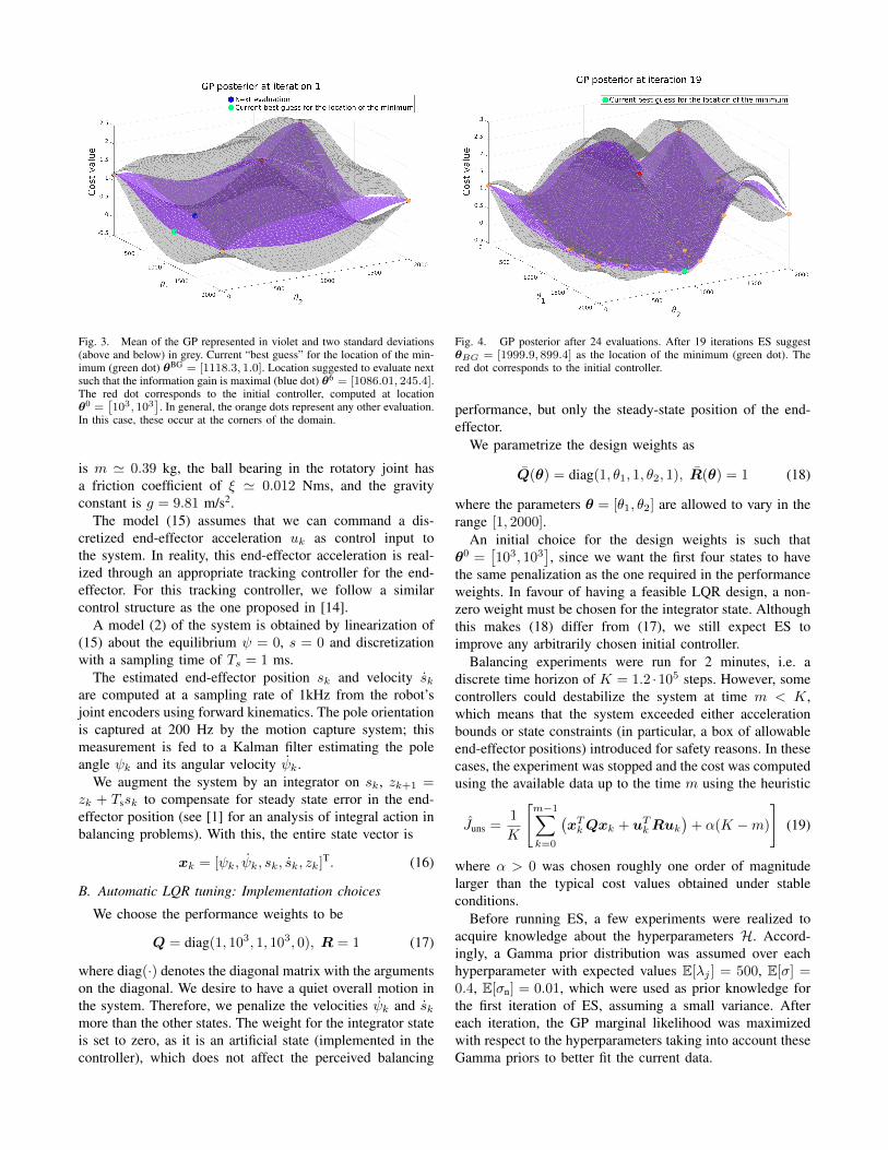
Fig. 3. Mean of the GP represented in violet and two standard deviations(above and below) in grey. Current “best guess” for the location of the min-imum (green dot) θBG = [1118.3, 1.0]. Location suggested to evaluate nextsuch that the information gain is maximal (blue dot) θ6 = [1086.01, 245.4].The red dot corresponds to the initial controller, computed at locationθ0 =

[103, 103

]. In general, the orange dots represent any other evaluation.

In this case, these occur at the corners of the domain.

is m ' 0.39 kg, the ball bearing in the rotatory joint hasa friction coefficient of ξ ' 0.012 Nms, and the gravityconstant is g = 9.81 m/s2.

The model (15) assumes that we can command a dis-cretized end-effector acceleration uk as control input tothe system. In reality, this end-effector acceleration is real-ized through an appropriate tracking controller for the end-effector. For this tracking controller, we follow a similarcontrol structure as the one proposed in [14].

A model (2) of the system is obtained by linearization of(15) about the equilibrium ψ = 0, s = 0 and discretizationwith a sampling time of Ts = 1 ms.

The estimated end-effector position sk and velocity skare computed at a sampling rate of 1kHz from the robot’sjoint encoders using forward kinematics. The pole orientationis captured at 200 Hz by the motion capture system; thismeasurement is fed to a Kalman filter estimating the poleangle ψk and its angular velocity ψk.

We augment the system by an integrator on sk, zk+1 =zk + Tssk to compensate for steady state error in the end-effector position (see [1] for an analysis of integral action inbalancing problems). With this, the entire state vector is

xk = [ψk, ψk, sk, sk, zk]T. (16)

B. Automatic LQR tuning: Implementation choices

We choose the performance weights to be

Q = diag(1, 103, 1, 103, 0), R = 1 (17)

where diag(·) denotes the diagonal matrix with the argumentson the diagonal. We desire to have a quiet overall motion inthe system. Therefore, we penalize the velocities ψk and skmore than the other states. The weight for the integrator stateis set to zero, as it is an artificial state (implemented in thecontroller), which does not affect the perceived balancing

Fig. 4. GP posterior after 24 evaluations. After 19 iterations ES suggestθBG = [1999.9, 899.4] as the location of the minimum (green dot). Thered dot corresponds to the initial controller.

performance, but only the steady-state position of the end-effector.

We parametrize the design weights as

Q(θ) = diag(1, θ1, 1, θ2, 1), R(θ) = 1 (18)

where the parameters θ = [θ1, θ2] are allowed to vary in therange [1, 2000].

An initial choice for the design weights is such thatθ0 =

[103, 103

], since we want the first four states to have

the same penalization as the one required in the performanceweights. In favour of having a feasible LQR design, a non-zero weight must be chosen for the integrator state. Althoughthis makes (18) differ from (17), we still expect ES toimprove any arbitrarily chosen initial controller.

Balancing experiments were run for 2 minutes, i.e. adiscrete time horizon of K = 1.2 ·105 steps. However, somecontrollers could destabilize the system at time m < K,which means that the system exceeded either accelerationbounds or state constraints (in particular, a box of allowableend-effector positions) introduced for safety reasons. In thesecases, the experiment was stopped and the cost was computedusing the available data up to the time m using the heuristic

Juns =1

K

[m−1∑k=0

(xTkQxk + uT

kRuk

)+ α(K −m)

](19)

where α > 0 was chosen roughly one order of magnitudelarger than the typical cost values obtained under stableconditions.

Before running ES, a few experiments were realized toacquire knowledge about the hyperparameters H. Accord-ingly, a Gamma prior distribution was assumed over eachhyperparameter with expected values E[λj ] = 500, E[σ] =0.4, E[σn] = 0.01, which were used as prior knowledge forthe first iteration of ES, assuming a small variance. Aftereach iteration, the GP marginal likelihood was maximizedwith respect to the hyperparameters taking into account theseGamma priors to better fit the current data.

TABLE ICOST VALUES FOR CASES 1 AND 2

J (Case 1) J (Case 2)mean std mean std

Initial set θ0 1.862 - 0.1958 0.02800Final best guess θBG 0.17556 0.0208 0.1648 0.02162

C. Results

We present the experimental results of two runs of theautomatic LQR tuning. In the first one, the model (2) hasbeen corrupted (significant underestimation of the dampingcoefficient) to provide more room for the auto-tuning. In thesecond one, we used the best available linear model.

Case 1: ES was initialized with five evaluations, i.e. theinitial controller θ0, and evaluations at the four cornersof the domain [1, 2000] × [1, 2000]. The initial controllerdestabilized the system and its cost was computed accordingto (19) with α = 1.5. Figure 3 shows the two-dimensionalGaussian process posterior after the five initial evaluations,which have relatively high cost values.

The algorithm can also work without evaluating initiallyat the corners of the domain; however, we found that theyprovide useful prestructuring of the GP and tend to speed upthe learning. This way, the algorithm focuses on interestingregions more quickly.

Executing Algorithm 1 for 19 iterations (i.e. 19 balancingexperiments) yielded the posterior GP illustrated in Fig. 4.The “best guess” θBG (green dot) is what ES suggests to bethe location of the minimum of the underlying cost (3).

To evaluate the result of the automatic LQR tuning, wecomputed the cost of the resulting controller (best guessafter 19 iterations) in five separate balancing experiments.The average and standard deviation of these experiments areshown in Table I (left), together with the cost value of theinitial controller (which was unstable in this case).

Case 2: In this experiment, the parameters of the modelwere not artificially modified, and the initial controller wasstable. After running Algorithm 1 for 27 iterations, ESsuggested θBG = [1402.1, 451, 6] as the best controller. Theresults of evaluating this controller five times, in comparisonto the initial controller, are shown in Table I (right). Albeitthe initial controller was obtained from the best linear modelwe had, the performance could still be improved by 15.9%.

V. CONCLUDING REMARKS

In this work, we introduce Entropy Search (ES), a globalBayesian optimization algorithm, for automatic controllertuning. We successfully demonstrated the developed tuningframework in experiments of a humanoid robot balancing aninverted pendulum. Improved controllers were obtained bothwhen the method was initialized with an unstable and witha stable controller.

The experiments herein represent early results, and weplan to do further tests in order to better evaluate thepotential of the proposed method. In particular, we planto investigate higher dimensional tuning problems (here,

only two parameters were varied) and cases where only acompletely wrong nominal model is given (here, only thedamping coefficient was corrupted). Since the ES algorithmreasons about where to evaluate next in order to maximize theinformation gain of an experiment, we expect the algorithmto make better use of the available data and yield improvedcontrollers more quickly than alternative approaches. Inves-tigating whether this claim holds in practice by comparingthe tuning performance of different methods is future work.

Another relevant direction for future extensions of theproposed method toward a truly automatic tool concerns theaspect of safety. While ES seeks to maximize the informa-tion obtained from an experiment, it seems reasonable toalso include safety considerations such as avoiding unstablecontrollers. Safe learning in the context of control is an areaof increasing interest and has recently been considered, e.g.,in [7], [15], [16] and [17] in slightly different contexts.

REFERENCES

[1] S. Trimpe and R. D’Andrea, “The Balancing Cube: A dynamicsculpture as test bed for distributed estimation and control,” IEEEControl Systems Magazine, vol. 32, no. 6, pp. 48–75, 2012.

[2] S. Mason, L. Righetti, and S. Schaal, “Full dynamics LQR control ofa humanoid robot: An experimental study on balancing and squatting,”in 14th IEEE-RAS International Conference on Humanoid Robots,2014, pp. 374–379.

[3] S. Trimpe, A. Millane, S. Doessegger, and R. D’Andrea, “A self-tuningLQR approach demonstrated on an inverted pendulum,” in IFAC WorldCongress, 2014, pp. 11 281–11 287.

[4] P. Hennig and C. J. Schuler, “Entropy search for information-efficientglobal optimization,” The Journal of Machine Learning Research,vol. 13, no. 1, pp. 1809–1837, 2012.

[5] J. W. Roberts, I. R. Manchester, and R. Tedrake, “Feedback controllerparameterizations for reinforcement learning,” in IEEE Symposium onAdaptive Dynamic Programming And Reinforcement Learning, 2011,pp. 310–317.

[6] J. Peters and S. Schaal, “Natural Actor-Critic,” Neurocomputing,vol. 71, no. 7, pp. 1180–1190, 2008.

[7] J. Schreiter, D. Nguyen-Tuong, M. Eberts, B. Bischoff, H. Markert,and M. Toussaint, “Safe exploration for active learning with Gaussianprocesses,” in European Conference on Machine Learning and Prin-ciples and Practice of Knowledge Discovery in Databases, 2015, toappear.

[8] B. D. Anderson and J. B. Moore, Optimal Control: Linear QuadraticMethods. Dover Publications, 1990.

[9] D. R. Jones, M. Schonlau, and W. J. Welch, “Efficient globaloptimization of expensive black-box functions,” Journal of GlobalOptimization, vol. 13, no. 4, pp. 455–492, 1998.

[10] D. J. Lizotte, “Practical bayesian optimization,” Ph.D. dissertation,2008.

[11] M. A. Osborne, R. Garnett, and S. J. Roberts, “Gaussian processesfor global optimization,” in 3rd International Conference on Learningand Intelligent Optimization, 2009, pp. 1–15.

[12] C. E. Rasmussen, “Gaussian processes for machine learning,” 2006.[13] S. Schaal, “Learning from demonstration,” Advances in Neural Infor-

mation Processing Systems, pp. 1040–1046, 1997.[14] L. Righetti, M. Kalakrishnan, P. Pastor, J. Binney, J. Kelly, R. C.

Voorhies, G. S. Sukhatme, and S. Schaal, “An autonomous manipu-lation system based on force control and optimization,” AutonomousRobots, vol. 36, no. 1-2, pp. 11–30, 2014.

[15] A. K. Akametalu, S. Kaynama, J. F. Fisac, M. N. Zeilinger, J. H.Gillula, and C. J. Tomlin, “Reachability-based safe learning withGaussian processes,” in IEEE 53rd Annual Conference on Decisionand Control, 2014, pp. 1424–1431.

[16] Y. Sui, A. Gotovos, J. Burdick, and A. Krause, “Safe explorationfor optimization with Gaussian processes,” in The 32nd InternationalConference on Machine Learning, 2015, pp. 997–1005.

[17] F. Berkenkamp and A. P. Schoellig, “Safe and robust learning controlwith Gaussian processes,” in European Control Conference, 2015.