automatic music transcription exploiting temporal …simond/phd/emmanouilbenetos-phd-thesis.pdf ·...
TRANSCRIPT
PhD thesis
Automatic Transcription of Polyphonic Music
Exploiting Temporal Evolution
Emmanouil Benetos
School of Electronic Engineering and Computer Science
Queen Mary University of London
2012

I certify that this thesis, and the research to which it refers, are the product
of my own work, and that any ideas or quotations from the work of other people,
published or otherwise, are fully acknowledged in accordance with the standard
referencing practices of the discipline. I acknowledge the helpful guidance and
support of my supervisor, Dr Simon Dixon.
i
Abstract
Automatic music transcription is the process of converting an audio recording
into a symbolic representation using musical notation. It has numerous ap-
plications in music information retrieval, computational musicology, and the
creation of interactive systems. Even for expert musicians, transcribing poly-
phonic pieces of music is not a trivial task, and while the problem of automatic
pitch estimation for monophonic signals is considered to be solved, the creation
of an automated system able to transcribe polyphonic music without setting
restrictions on the degree of polyphony and the instrument type still remains
open.
In this thesis, research on automatic transcription is performed by explicitly
incorporating information on the temporal evolution of sounds. First efforts ad-
dress the problem by focusing on signal processing techniques and by proposing
audio features utilising temporal characteristics. Techniques for note onset and
offset detection are also utilised for improving transcription performance. Sub-
sequent approaches propose transcription models based on shift-invariant prob-
abilistic latent component analysis (SI-PLCA), modeling the temporal evolution
of notes in a multiple-instrument case and supporting frequency modulations in
produced notes. Datasets and annotations for transcription research have also
been created during this work. Proposed systems have been privately as well as
publicly evaluated within the Music Information Retrieval Evaluation eXchange
(MIREX) framework. Proposed systems have been shown to outperform several
state-of-the-art transcription approaches.
Developed techniques have also been employed for other tasks related to mu-
sic technology, such as for key modulation detection, temperament estimation,
and automatic piano tutoring. Finally, proposed music transcription models
have also been utilized in a wider context, namely for modeling acoustic scenes.

Acknowledgements
First and foremost, I would like to thank my supervisor, Simon Dixon, for three
years of sound advice, his cheerful disposition, for providing me with a great
deal of freedom to explore the topics of my choice and work on the research
areas that interest me the most. I would like to also thank Anssi Klapuri and
Mark Plumbley for their extremely detailed feedback, and for their useful advice
that helped shape my research.
A big thanks to the members (past and present) of the Centre for Digital
Music who have made these three years easily my most pleasant research ex-
perience. Special thanks to Amelie Anglade, Matthias Mauch, Lesley Mearns,
Dan Tidhar, Dimitrios Giannoulis, Holger Kirchhoff, and Dan Stowell for their
expertise and help that has led to joint publications and work. Thanks also
to Mathieu Lagrange for a very nice stay at IRCAM and to Arshia Cont for
making it possible.
There are so many other people from C4DM that I am grateful to, including
(but not limited to): Daniele Barchiesi, Mathieu Barthet, Magdalena Chudy,
Alice Clifford, Matthew Davies, Joachim Ganseman, Steven Hargreaves, Robert
Macrae, Boris Mailhe, Martin Morrell, Katy Noland, Ken O’Hanlon, Steve Wel-
burn, and Asterios Zacharakis. Thanks also to the following non-C4DM people
for helping me with my work: Gautham Mysore, Masahiro Nakano, Romain
Hennequin, Piotr Holonowicz, and Valentin Emiya.
I would like to also thank the people from the QMUL IEEE student branch:
Yiannis Patras, Sohaib Qamer, Xian Zhang, Yading Song, Ammar Lilamwala,
Bob Chew, Sabri-E-Zaman, Amna Wahid, and Roya Haratian. A big thanks to
Margarita for the support and the occasional proofreading! Many thanks finally
to my family and friends for simply putting up with me all this time!
This work was funded by a Queen Mary University of London Westfield
Trust Research Studentship.
iii
Contents
1 Introduction 1
1.1 Motivation and aim . . . . . . . . . . . . . . . . . . . . . . . . . 1
1.2 Thesis structure . . . . . . . . . . . . . . . . . . . . . . . . . . . . 3
1.3 Contributions . . . . . . . . . . . . . . . . . . . . . . . . . . . . . 4
1.4 Associated publications . . . . . . . . . . . . . . . . . . . . . . . 6
2 Background 9
2.1 Terminology . . . . . . . . . . . . . . . . . . . . . . . . . . . . . . 9
2.1.1 Music Signals . . . . . . . . . . . . . . . . . . . . . . . . . 9
2.1.2 Tonality . . . . . . . . . . . . . . . . . . . . . . . . . . . . 11
2.1.3 Rhythm . . . . . . . . . . . . . . . . . . . . . . . . . . . . 14
2.1.4 MIDI Notation . . . . . . . . . . . . . . . . . . . . . . . . 15
2.2 Single-pitch Estimation . . . . . . . . . . . . . . . . . . . . . . . 16
2.2.1 Spectral Methods . . . . . . . . . . . . . . . . . . . . . . . 17
2.2.2 Temporal Methods . . . . . . . . . . . . . . . . . . . . . . 19
2.2.3 Spectrotemporal Methods . . . . . . . . . . . . . . . . . . 19
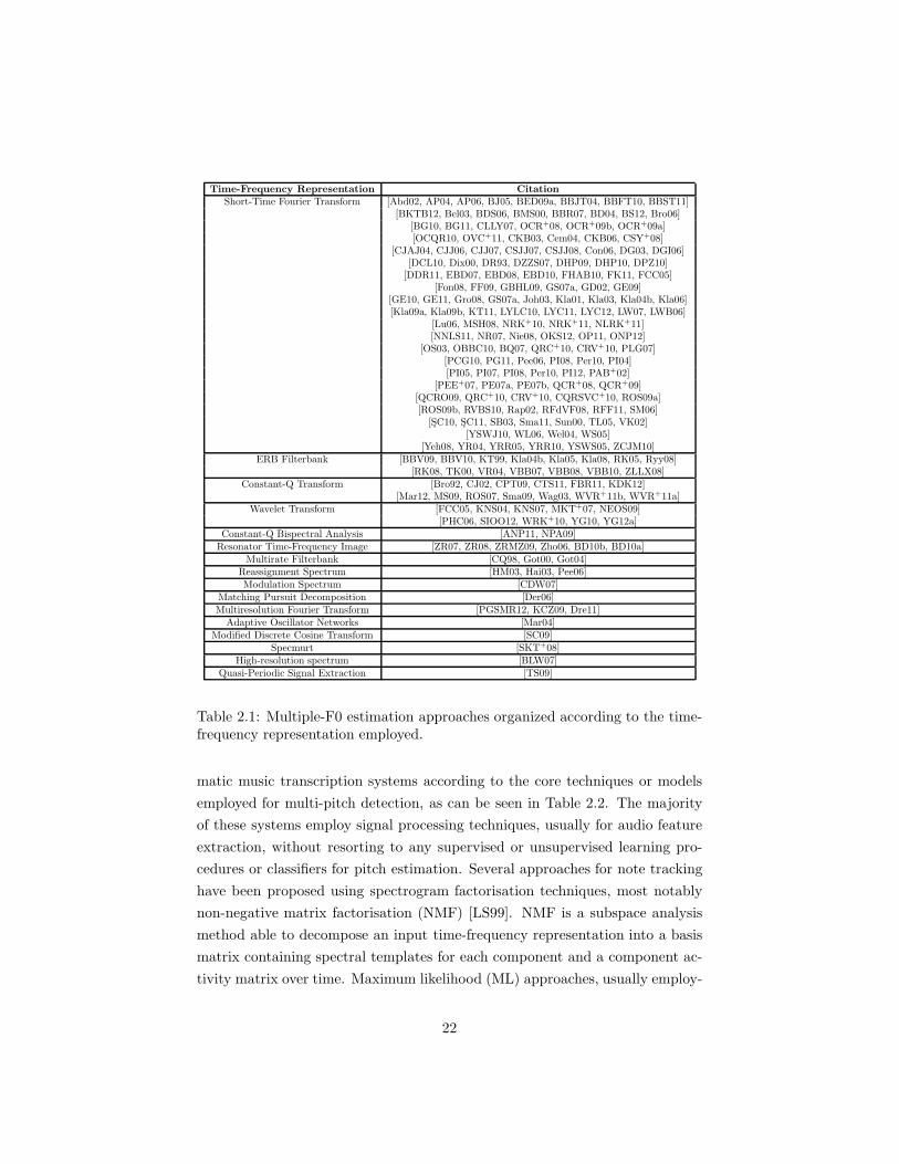
2.3 Multi-pitch Estimation and Polyphonic Music Transcription . . . 20
2.3.1 Signal Processing Methods . . . . . . . . . . . . . . . . . 23
2.3.2 Statistical Modelling Methods . . . . . . . . . . . . . . . . 28
2.3.3 Spectrogram Factorization Methods . . . . . . . . . . . . 31
2.3.4 Sparse Methods . . . . . . . . . . . . . . . . . . . . . . . . 43
2.3.5 Machine Learning Methods . . . . . . . . . . . . . . . . . 45
2.3.6 Genetic Algorithm Methods . . . . . . . . . . . . . . . . . 47
2.4 Note Tracking . . . . . . . . . . . . . . . . . . . . . . . . . . . . . 47
2.5 Evaluation metrics . . . . . . . . . . . . . . . . . . . . . . . . . . 49
2.5.1 Frame-based Evaluation . . . . . . . . . . . . . . . . . . . 49
2.5.2 Note-based Evaluation . . . . . . . . . . . . . . . . . . . . 51
iv
2.6 Public Evaluation . . . . . . . . . . . . . . . . . . . . . . . . . . . 52
2.7 Discussion . . . . . . . . . . . . . . . . . . . . . . . . . . . . . . . 53
2.7.1 Assumptions . . . . . . . . . . . . . . . . . . . . . . . . . 53
2.7.2 Design Considerations . . . . . . . . . . . . . . . . . . . . 56
2.7.3 Towards a Complete Transcription . . . . . . . . . . . . . 57
3 Audio Feature-based Automatic Music Transcription 59
3.1 Introduction . . . . . . . . . . . . . . . . . . . . . . . . . . . . . . 59
3.2 Multiple-F0 Estimation of Piano Sounds . . . . . . . . . . . . . . 60
3.2.1 Preprocessing . . . . . . . . . . . . . . . . . . . . . . . . . 61
3.2.2 Multiple-F0 Estimation . . . . . . . . . . . . . . . . . . . 62
3.3 Joint Multiple-F0 Estimation for AMT . . . . . . . . . . . . . . . 68
3.3.1 Preprocessing . . . . . . . . . . . . . . . . . . . . . . . . . 68
3.3.2 Multiple-F0 Estimation . . . . . . . . . . . . . . . . . . . 70
3.3.3 Postprocessing . . . . . . . . . . . . . . . . . . . . . . . . 75
3.4 AMT using Note Onset and Offset Detection . . . . . . . . . . . 78
3.4.1 Preprocessing . . . . . . . . . . . . . . . . . . . . . . . . . 79
3.4.2 Onset Detection . . . . . . . . . . . . . . . . . . . . . . . 79
3.4.3 Multiple-F0 Estimation . . . . . . . . . . . . . . . . . . . 81
3.4.4 Offset Detection . . . . . . . . . . . . . . . . . . . . . . . 82
3.5 Evaluation . . . . . . . . . . . . . . . . . . . . . . . . . . . . . . . 83
3.5.1 Datasets . . . . . . . . . . . . . . . . . . . . . . . . . . . . 83
3.5.2 Results . . . . . . . . . . . . . . . . . . . . . . . . . . . . 86
3.6 Discussion . . . . . . . . . . . . . . . . . . . . . . . . . . . . . . . 95
4 Spectrogram Factorization-based Automatic Music Transcrip-
tion 97
4.1 Introduction . . . . . . . . . . . . . . . . . . . . . . . . . . . . . . 97
4.2 AMT using a Convolutive Probabilistic Model . . . . . . . . . . . 98
4.2.1 Formulation . . . . . . . . . . . . . . . . . . . . . . . . . . 99
4.2.2 Parameter Estimation . . . . . . . . . . . . . . . . . . . . 100
4.2.3 Sparsity constraints . . . . . . . . . . . . . . . . . . . . . 101
4.2.4 Postprocessing . . . . . . . . . . . . . . . . . . . . . . . . 103
4.3 Pitch Detection using a Temporally-constrained Convolutive Prob-
abilistic Model . . . . . . . . . . . . . . . . . . . . . . . . . . . . 104
4.3.1 Formulation . . . . . . . . . . . . . . . . . . . . . . . . . . 105
4.3.2 Parameter Estimation . . . . . . . . . . . . . . . . . . . . 106
v

4.4 AMT using a Temporally-constrained Convolutive Probabilistic
Model . . . . . . . . . . . . . . . . . . . . . . . . . . . . . . . . . 108
4.4.1 Formulation . . . . . . . . . . . . . . . . . . . . . . . . . . 109
4.4.2 Parameter Estimation . . . . . . . . . . . . . . . . . . . . 111
4.4.3 Sparsity constraints . . . . . . . . . . . . . . . . . . . . . 113
4.4.4 Postprocessing . . . . . . . . . . . . . . . . . . . . . . . . 115
4.5 Evaluation . . . . . . . . . . . . . . . . . . . . . . . . . . . . . . . 115
4.5.1 Training Data . . . . . . . . . . . . . . . . . . . . . . . . . 115
4.5.2 Test Data . . . . . . . . . . . . . . . . . . . . . . . . . . . 117
4.5.3 Results . . . . . . . . . . . . . . . . . . . . . . . . . . . . 117
4.6 Discussion . . . . . . . . . . . . . . . . . . . . . . . . . . . . . . . 129
5 Transcription Applications 132
5.1 Automatic Detection of Key Modulations in J.S. Bach Chorales . 133
5.1.1 Motivation . . . . . . . . . . . . . . . . . . . . . . . . . . 133
5.1.2 Music Transcription . . . . . . . . . . . . . . . . . . . . . 134
5.1.3 Chord Recognition . . . . . . . . . . . . . . . . . . . . . . 135
5.1.4 Key Modulation Detection . . . . . . . . . . . . . . . . . 136
5.1.5 Evaluation . . . . . . . . . . . . . . . . . . . . . . . . . . 137
5.1.6 Discussion . . . . . . . . . . . . . . . . . . . . . . . . . . . 137
5.2 Harpsichord-specific Transcription for Temperament Estimation . 138
5.2.1 Background . . . . . . . . . . . . . . . . . . . . . . . . . . 138
5.2.2 Dataset . . . . . . . . . . . . . . . . . . . . . . . . . . . . 139
5.2.3 Harpsichord Transcription . . . . . . . . . . . . . . . . . . 139
5.2.4 Precise F0 and Temperament Estimation . . . . . . . . . 141
5.2.5 Evaluation and Discussion . . . . . . . . . . . . . . . . . . 142
5.3 Score-informed Transcription for Automatic Piano Tutoring . . . 143
5.3.1 MIDI-to-audio Alignment and Synthesis . . . . . . . . . . 143
5.3.2 Multi-pitch Detection . . . . . . . . . . . . . . . . . . . . 144
5.3.3 Note Tracking . . . . . . . . . . . . . . . . . . . . . . . . 145
5.3.4 Piano-roll Comparison . . . . . . . . . . . . . . . . . . . . 145
5.3.5 Evaluation . . . . . . . . . . . . . . . . . . . . . . . . . . 147
5.3.6 Discussion . . . . . . . . . . . . . . . . . . . . . . . . . . . 150
5.4 Characterisation of Acoustic Scenes using SI-PLCA . . . . . . . . 151
5.4.1 Background . . . . . . . . . . . . . . . . . . . . . . . . . . 151
5.4.2 Proposed Method . . . . . . . . . . . . . . . . . . . . . . . 152
5.4.3 Evaluation . . . . . . . . . . . . . . . . . . . . . . . . . . 156
vi

5.4.4 Discussion . . . . . . . . . . . . . . . . . . . . . . . . . . . 160
5.5 Discussion . . . . . . . . . . . . . . . . . . . . . . . . . . . . . . . 161
6 Conclusions and Future Perspectives 163
6.1 Summary . . . . . . . . . . . . . . . . . . . . . . . . . . . . . . . 163
6.1.1 Audio feature-based AMT . . . . . . . . . . . . . . . . . . 163
6.1.2 Spectrogram factorization-based AMT . . . . . . . . . . . 164
6.1.3 Transcription Applications . . . . . . . . . . . . . . . . . 166
6.2 Future Perspectives . . . . . . . . . . . . . . . . . . . . . . . . . . 167
A Expected Value of Noise Log-Amplitudes 170
B Log-frequency spectral envelope estimation 171
C Derivations for the Temporally-constrained Convolutive Model174
C.1 Log likelihood . . . . . . . . . . . . . . . . . . . . . . . . . . . . . 175
C.2 Expectation Step . . . . . . . . . . . . . . . . . . . . . . . . . . . 177
C.3 Maximization Step . . . . . . . . . . . . . . . . . . . . . . . . . . 179
vii

List of Figures
1.1 An automatic music transcription example. . . . . . . . . . . . . 3
2.1 A D3 piano note (146.8 Hz). . . . . . . . . . . . . . . . . . . . . . 11
2.2 The spectrogram of an A3 marimba note. . . . . . . . . . . . . . 12
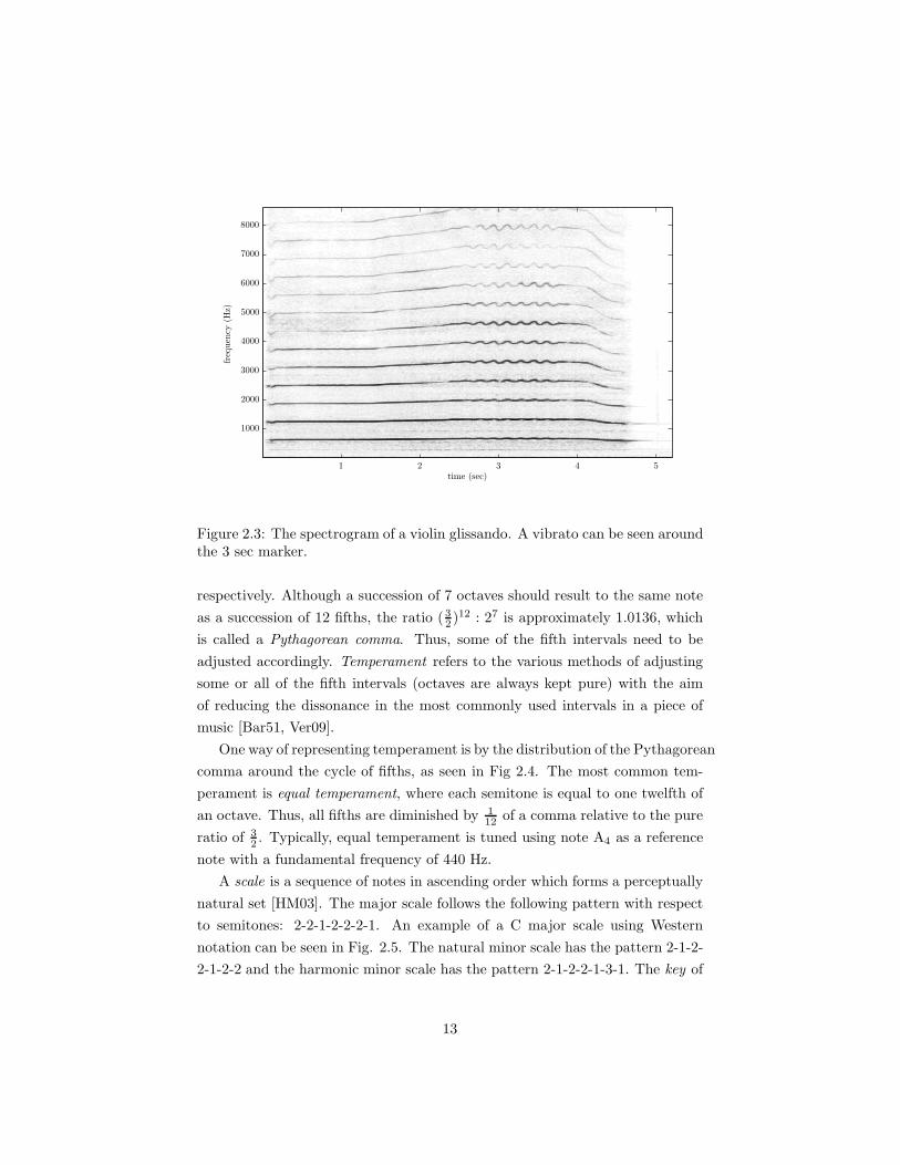
2.3 The spectrogram of a violin glissando. . . . . . . . . . . . . . . . 13
2.4 Circle of fifths representation for the ‘Sixth comma meantone‘
and ‘Fifth comma‘ temperaments. . . . . . . . . . . . . . . . . . 14
2.5 A C major scale, starting from C4 and finishing at C5. . . . . . . 14
2.6 The opening bars of J.S. Bach’s menuet in G major (BWV Anh.
114) illustrating the three metrical levels. . . . . . . . . . . . . . 15
2.7 The piano-roll representation of J.S. Bach’s prelude in C major
from the Well-tempered Clavier. . . . . . . . . . . . . . . . . . . 16
2.8 The spectrum of a C4 piano note . . . . . . . . . . . . . . . . . . 17
2.9 The constant-Q transform spectrum of a C4 piano note (sample
from MAPS database [EBD10]). . . . . . . . . . . . . . . . . . . 18
2.10 Pitch detection using the unitary model of [MO97]. . . . . . . . . 20
2.11 The iterative spectral subtraction system of Klapuri (figure from
[Kla03]). . . . . . . . . . . . . . . . . . . . . . . . . . . . . . . . . 25
2.12 Example of the Gaussian smoothing procedure of [PI08] for a
harmonic partial sequence. . . . . . . . . . . . . . . . . . . . . . . 26
2.13 The RFTI spectrum of a C4 piano note. . . . . . . . . . . . . . . 27
2.14 An example of the tone model of [Got04]. . . . . . . . . . . . . . 29
2.15 The NMF algorithm with Z = 5 applied to the opening bars
of J.S. Bach’s English Suite No. 5 (BWV 810 - recording from
[Mar04]). . . . . . . . . . . . . . . . . . . . . . . . . . . . . . . . 33
2.16 The activation matrix of the NMF algorithm with β-divergence
applied to the recording of Fig. 2.15. . . . . . . . . . . . . . . . . 35
viii
2.17 An example of PLCA applied to a C4 piano note. . . . . . . . . . 39
2.18 An example of SI-PLCA applied to a cello melody. . . . . . . . . 41
2.19 An example of a non-negative hidden Markov model using a left-
to-right HMM with 3 states. . . . . . . . . . . . . . . . . . . . . . 43
2.20 System diagram of the piano transcription method in [BS12]. . . 47
2.21 Graphical structure of the pitch-wise HMM of [PE07a]. . . . . . 49
2.22 An example of the note tracking procedure of [PE07a]. . . . . . . 50
2.23 Trumpet (a) and clarinet (b) spectra of a C4 tone (261Hz). . . . 55
3.1 Diagram for the proposed multiple-F0 estimation system for iso-
lated piano sounds. . . . . . . . . . . . . . . . . . . . . . . . . . . 60
3.2 (a) The RTFI slice Y [ω] of an F♯3 piano sound. (b) The corre-
sponding pitch salience function S ′[p]. . . . . . . . . . . . . . . . 64
3.3 Salience function stages for an E4-G4-B4-C5-D5 piano chord. . 67
3.4 Diagram for the proposed joint multiple-F0 estimation system for
automatic music transcription. . . . . . . . . . . . . . . . . . . . 68
3.5 Transcription output of an excerpt of ‘RWC MDB-J-2001 No. 2’
(jazz piano). . . . . . . . . . . . . . . . . . . . . . . . . . . . . . . 76
3.6 Graphical structure of the postprocessing decoding process for
(a) HMM (b) Linear chain CRF networks. . . . . . . . . . . . . . 78
3.7 An example for the complete transcription system of Section 3.4,
from preprocessing to offset detection. . . . . . . . . . . . . . . . 83
3.8 Multiple-F0 estimation results for the MAPS database (in F-
measure) with unknown polyphony. . . . . . . . . . . . . . . . . . 87
4.1 Diagram for the proposed automatic transcription system using
a convolutive probabilistic model. . . . . . . . . . . . . . . . . . . 99
4.2 (a) The pitch activity matrix P (p, t) of the first 23s of of ‘RWC
MDB-J-2001 No. 9’ (guitar). (b) The pitch ground truth of the
same recording. . . . . . . . . . . . . . . . . . . . . . . . . . . . . 102
4.3 The time-pitch representation P (f ′, t) of the first 23s of ‘RWC
MDB-C-2001 No. 12’ (string quartet). . . . . . . . . . . . . . . . 103
4.4 The pitch activity matrix and the piano-roll transcription matrix
derived from the HMM postprocessing step for the first 23s of
‘RWC MDB-C-2001 No. 30’ (piano). . . . . . . . . . . . . . . . . 105
4.5 An example of the single-source temporally-constrained convolu-
tive model. . . . . . . . . . . . . . . . . . . . . . . . . . . . . . . 109
ix

4.6 Time-pitch representation P (f ′, t) of an excerpt of “RWC-MDB-
J-2001 No. 7” (guitar). . . . . . . . . . . . . . . . . . . . . . . . . 112
4.7 Log-likelihood evolution using different sparsity values for ‘RWC-
MDB-J-2001 No.1’ (piano). . . . . . . . . . . . . . . . . . . . . . 114
4.8 An example of the HMM-based note tracking step for the model
of Section 4.4. . . . . . . . . . . . . . . . . . . . . . . . . . . . . . 116
4.9 The model of Section 4.3 applied to a piano melody. . . . . . . . 119
4.10 Transcription results (Acc2) for the system of Section 4.2 for RWC
recordings 1-12 using various sparsity parameters (while the other
parameter is set to 1.0). . . . . . . . . . . . . . . . . . . . . . . . 123
4.11 Transcription results (Acc2) for the system of Section 4.4 for RWC
recordings 1-12 using various sparsity parameters (while the other
parameter is set to 1.0). . . . . . . . . . . . . . . . . . . . . . . . 124
4.12 Instrument assignment results (F) for the method of Section 4.2
using the first 30 sec of the MIREX woodwind quintet. . . . . . . 127
4.13 Instrument assignment results (F) for the method of Section 4.4
using the first 30 sec of the MIREX woodwind quintet. . . . . . . 128
5.1 Key modulation detection diagram. . . . . . . . . . . . . . . . . . 133
5.2 Transcription of the BWV 2.6 ‘Ach Gott, vom Himmel sieh’
darein’ chorale. . . . . . . . . . . . . . . . . . . . . . . . . . . . . 135
5.3 Transcription of J.S. Bach’s Menuet in G minor (RWC MDB-C-
2001 No. 24b). . . . . . . . . . . . . . . . . . . . . . . . . . . . . 141
5.4 Diagram for the proposed score-informed transcription system. . 143
5.5 The score-informed transcription of a segment from Johann Krieger’s
Bourree. . . . . . . . . . . . . . . . . . . . . . . . . . . . . . . . . 147
5.6 Diagram for the proposed acoustic scene characterisation system. 153
5.7 Acoustic scene classification results (MAP) using (a) the SI-PLCA
algorithm (b) the TCSI-PLCA algorithm, with different sparsity
parameter (sH) and dictionary size (Z). . . . . . . . . . . . . . 158
B.1 Log-frequency spectral envelope of an F#4 piano tone with P =
50. The circle markers correspond to the detected overtones. . . 173
x
List of Tables
2.1 Multiple-F0 estimation approaches organized according to the
time-frequency representation employed. . . . . . . . . . . . . . . 22
2.2 Multiple-F0 and note tracking techniques organised according to
the employed technique. . . . . . . . . . . . . . . . . . . . . . . . 24
2.3 Best results for the MIREXMulti-F0 estimation task [MIR], from
2009-2011, using the accuracy and chroma accuracy metrics. . . . 53
3.1 The RWC data used for transcription experiments. . . . . . . . . 85
3.2 The piano dataset created in [PE07a], which is used for transcrip-
tion experiments. . . . . . . . . . . . . . . . . . . . . . . . . . . . 86
3.3 Transcription results (Acc2) for the RWC recordings 1-12. . . . . 89
3.4 Transcription results (Acc2) for RWC recordings 13-17. . . . . . . 90
3.5 Transcription error metrics for the proposed method using RWC
recordings 1-17. . . . . . . . . . . . . . . . . . . . . . . . . . . . . 91
3.6 Transcription results (Acc2) for the RWC recordings 1-12 using
the method in §3.3, when features are removed from the score
function (3.17). . . . . . . . . . . . . . . . . . . . . . . . . . . . . 91
3.7 Mean transcription results (Acc1) for the recordings from [PE07a]. 92
3.8 Transcription error metrics using the recordings from [PE07a]. . 93
3.9 Transcription error metrics using the MIREX multiF0 recording. 93
3.10 MIREX 2010 multiple-F0 estimation results for the submitted
system. . . . . . . . . . . . . . . . . . . . . . . . . . . . . . . . . 94
3.11 MIREX 2010 multiple-F0 estimation results in terms of accuracy
and chroma accuracy for all submitted systems. . . . . . . . . . . 94
4.1 MIDI note range of the instruments employed for note and sound
state template extraction. . . . . . . . . . . . . . . . . . . . . . . 117
xi

4.2 Pitch detection results using the proposed method of Section
4.3 with left-to-right and ergodic HMMs, compared with the SI-
PLCA method. . . . . . . . . . . . . . . . . . . . . . . . . . . . . 120
4.3 Transcription results (Acc2) for the RWC recordings 1-12. . . . . 121
4.4 Transcription results (Acc2) for RWC recordings 13-17. . . . . . . 121
4.5 Transcription error metrics for the proposed methods using RWC
recordings 1-17. . . . . . . . . . . . . . . . . . . . . . . . . . . . . 122
4.6 Mean transcription results (Acc1 ) for the piano recordings from
[PE07a]. . . . . . . . . . . . . . . . . . . . . . . . . . . . . . . . . 123
4.7 Transcription error metrics for the piano recordings in [PE07a]. . 124
4.8 Frame-based F for the first 30 sec of the MIREX woodwind quin-
tet, comparing the proposed methods with other approaches. . . 125
4.9 Transcription error metrics for the complete MIREX woodwind
quintet. . . . . . . . . . . . . . . . . . . . . . . . . . . . . . . . . 126
4.10 MIREX 2011 multiple-F0 estimation results for the submitted
system. . . . . . . . . . . . . . . . . . . . . . . . . . . . . . . . . 129
4.11 MIREX 2011 multiple-F0 estimation results in terms of accuracy
and chroma accuracy for all submitted systems. . . . . . . . . . . 129
4.12 MIREX 2011 note tracking results for all submitted systems. . . 130
5.1 The list of J.S. Bach chorales used for the key modulation detec-
tion experiments. . . . . . . . . . . . . . . . . . . . . . . . . . . . 134
5.2 Chord match results for the six transcribed audio and ground
truth MIDI against hand annotations. . . . . . . . . . . . . . . . 136
5.3 The score-informed piano transcription dataset. . . . . . . . . . . 148
5.4 Automatic transcription results for score-informed transcription
dataset. . . . . . . . . . . . . . . . . . . . . . . . . . . . . . . . . 149
5.5 Score-informed transcription results. . . . . . . . . . . . . . . . . 150
5.6 Class distribution in the employed dataset of acoustic scenes. . . 157
5.7 Best MAP and 5-precision results for each model. . . . . . . . . . 159
5.8 Best classification accuracy for each model. . . . . . . . . . . . . 160
xii
List of Abbreviations
ALS Alternating Least Squares
AMT Automatic Music Transcription
ARMA AutoRegressive Moving Average
ASR Automatic Speech Recognition
BLSTM Bidirectional Long Short-Term Memory
BOF Bag-of-frames
CAM Common Amplitude Modulation
CASA Computational Auditory Scene Analysis
CQT Constant-Q Transform
CRF Conditional Random Fields
DBNs Dynamic Bayesian Networks
DFT Discrete Fourier Transform
EM Expectation Maximization
ERB Equivalent Rectangular Bandwidth
FFT Fast Fourier Transform
GMMs Gaussian Mixture Models
HMMs Hidden Markov Models
HMP Harmonic Matching Pursuit
HNNMA Harmonic Non-Negative Matrix Approximation
HPS Harmonic Partial Sequence
KL Kullback-Leibler
MAP Maximum A Posteriori
MCMC Markov Chain Monte Carlo
MFCC Mel-Frequency Cepstral Coefficient
MIR Music Information Retrieval
ML Maximum Likelihood
MP Matching Pursuit
xiii

MUSIC MUltiple Signal Classification
NHMM Non-negative Hidden Markov Model
NMD Non-negative Matrix Deconvolution
NMF Non-negative Matrix Factorization
PDF Probability Density Function
PLCA Probabilistic Latent Component Analysis
PLTF Probabilistic Latent Tensor Factorization
RTFI Resonator Time-Frequency Image
SI-PLCA Shift-Invariant Probabilistic Latent Component Analysis
STFT Short-Time Fourier Transform
SVMs Support Vector Machines
TCSI-PLCA Temporally-constrained SI-PLCA
TDNNs Time-Delay Neural Networks
VB Variational Bayes
xiv

List of Variables
a partial amplitude
αt(qt) forward variable
bp inharmonicity parameter for pitch p
B RTFI segment for CAM feature
βt(qt) backward variable
β beta-divergence
C Set of all possible f0 combinations
δp tuning deviation for pitch p
χ exponential distribution parameter
dz(l,m) distance between acoustic scenes l and m for component z
D(l,m) distance between two acoustic scenes l and m
∆φ phase difference
f0 fundamental frequency
f pitch impulse used in convolutive models
fp,h frequency for h-th harmonic of p-th pitch
γ Euler constant
h partial index
H activation matrix in NMF-based models
HPS [p, h] harmonic partial sequence
j spectral whitening parameter
λ note tracking parameter
L maximum polyphony level
µ shifted log-frequency index for shift-invariant model
ν time lag
N [ω, t] RTFI noise estimate
ω frequency index
Ω maximum frequency index
xv

o observation in HMMs for note tracking
p pitch
p chroma index
ψ[p, t] Semitone-resolution filterbank for onset detection
P (·) probability
q state in NHMM and variants for AMT
q state in HMMs for note tracking
ρ sparsity parameter in [Sma11]
ρ1 sparsity parameter for source contribution
ρ2 sparsity parameter for pitch activation
peak scaling value for spectral whitening
s Source index
S Number of sources
S[p] pitch salience function
t time index
T Time length
τ Shift in NMD model [Sma04a]
θ floor parameter for spectral whitening
u number of bins per octave
V spectrogram matrix in NMF-based models
Vω,t spectrogram value at ω-th frequency and t-th frame
v spectral frame
W basis matrix in NMF-based models
x[n] discrete (sampled) domain signal
ξ cepstral coefficient index
X [ω, t] Absolute value of RTFI
Y [ω, t] Whitened RTFI
z component index
Z number of components
xvi
Chapter 1
Introduction
The topic of this thesis is automatic transcription of polyphonic music exploiting
temporal evolution. This chapter explains the motivations and aim (Section 1.1)
of this work. Also, the structure of the thesis is provided (Section 1.2) along
with the main contributions of this work (Section 1.3). Finally, publications
associated with the thesis are listed in Section 1.4.
1.1 Motivation and aim
Automatic music transcription (AMT) is the process of converting an audio
recording into a symbolic representation using some form of musical notation.
Even for expert musicians, transcribing polyphonic pieces of music is not a trivial
task [KD06], and while the problem of automatically transcribing monophonic
signals is considered to be a solved problem, the creation of an automated system
able to transcribe polyphonic music without setting restrictions on the degree
of polyphony and the instrument type still remains open. The most immediate
application of automatic music transcription is for allowing musicians to store
and reproduce a recorded performance [Kla04b]. In the past years, the problem
of automatic music transcription has gained considerable research interest due
to the numerous applications associated with the area, such as automatic search
and annotation of musical information, interactive music systems (e.g. computer
participation in live human performances, score following, and rhythm tracking),
as well as musicological analysis [Bel03, Got04, KD06].
The AMT problem can be divided into several subtasks, which include: pitch
1
estimation, onset/offset detection, loudness estimation, instrument recognition,
and extraction of rhythmic information. The core problem in automatic tran-
scription is the estimation of concurrent pitches in a time frame, also called
multiple-F0 or multi-pitch estimation. As mentioned in [Cem04], automatic mu-
sic transcription in the research literature is defined as the process of converting
an audio recording into piano-roll notation, while the process of converting a
piano-roll into a human readable score is viewed as a separate problem. The 1st
process involves tasks such as pitch estimation, note tracking, and instrument
identification, while the 2nd process involves tasks such as rhythmic parsing,
key induction, and note grouping.
For an overview of transcription approaches, the reader is referred to [KD06],
while in [dC06] a review of multiple fundamental frequency estimation systems
is given. A more recent overview of multi-pitch estimation and transcription
is given in [MEKR11], while [BDG+12] presents future directions in AMT re-
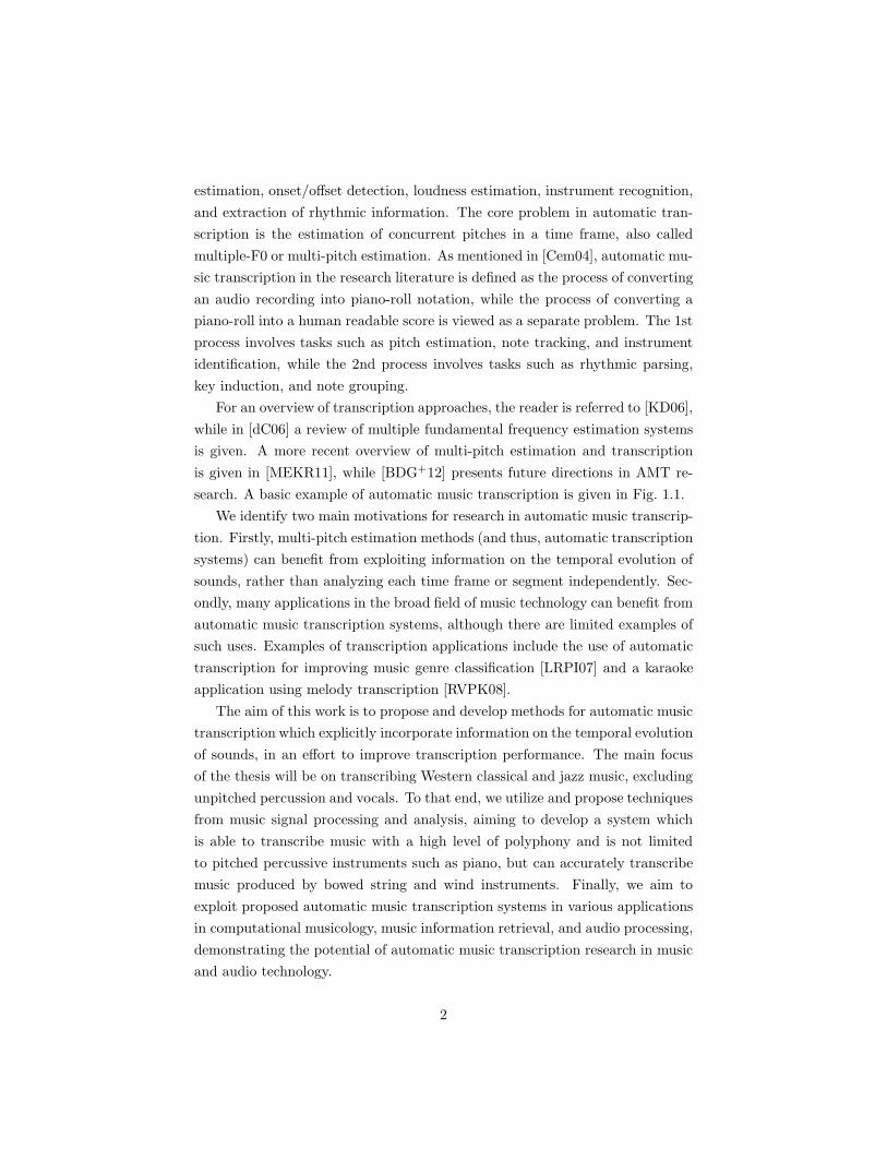
search. A basic example of automatic music transcription is given in Fig. 1.1.
We identify two main motivations for research in automatic music transcrip-
tion. Firstly, multi-pitch estimation methods (and thus, automatic transcription
systems) can benefit from exploiting information on the temporal evolution of
sounds, rather than analyzing each time frame or segment independently. Sec-
ondly, many applications in the broad field of music technology can benefit from
automatic music transcription systems, although there are limited examples of
such uses. Examples of transcription applications include the use of automatic
transcription for improving music genre classification [LRPI07] and a karaoke
application using melody transcription [RVPK08].
The aim of this work is to propose and develop methods for automatic music
transcription which explicitly incorporate information on the temporal evolution
of sounds, in an effort to improve transcription performance. The main focus
of the thesis will be on transcribing Western classical and jazz music, excluding
unpitched percussion and vocals. To that end, we utilize and propose techniques
from music signal processing and analysis, aiming to develop a system which
is able to transcribe music with a high level of polyphony and is not limited
to pitched percussive instruments such as piano, but can accurately transcribe
music produced by bowed string and wind instruments. Finally, we aim to
exploit proposed automatic music transcription systems in various applications
in computational musicology, music information retrieval, and audio processing,
demonstrating the potential of automatic music transcription research in music
and audio technology.
2
Figure 1.1: An automatic music transcription example. The top part of thefigure contains a waveform segment from a recording of J.S. Bach’s Prelude inD major from the Well-Tempered Clavier Book I, performed on a piano. In themiddle figure, a time-frequency representation of the signal can be seen, withdetected pitches in rectangles (using the transcription method of [DCL10]). Thebottom part of the figure shows the corresponding score.
1.2 Thesis structure
Chapter 2 presents an overview of related work on automatic music transcrip-
tion. It begins with a presentation of basic concepts from music terminol-
ogy. Afterwards the problem of automatic music transcription is defined,
followed by related work on single-pitch detection. Finally, a detailed sur-
vey on state-of-the-art automatic transcription methods for polyphonic
music is presented.
Chapter 3 presents proposed methods for audio feature-based automatic mu-
sic transcription. Preliminary work on multiple-F0 estimation on isolated
piano chords is described, followed by an automatic music transcription
3

system for polyphonic music. The latter system utilizes audio features
exploiting temporal evolution. Finally, a transcription system which also
incorporates information on note onsets and offsets is given. Private and
public evaluation results using the proposed methods are given.
Chapter 4 presents proposed methods for automatic music transcription which
are based on spectrogram factorization techniques. More specifically, a
transcription model which is based on shift-invariant probabilistic latent
component analysis (SI-PLCA) is presented. Further work focuses on
modeling the temporal evolution of sounds within the SI-PLCA frame-
work, where a single-pitch model is presented followed by a multi-pitch,
multi-instrument model for music transcription. Private and public eval-
uation results using the proposed methods are given.
Chapter 5 presents applications of proposed transcription systems. Proposed
systems have been utilized in computational musicology applications, in-
cluding key modulation detection in J.S. Bach chorales and temperament
estimation in harpsichord recordings. A system for score-informed tran-
scription has also been proposed, applied to automatic piano tutoring.
Proposed transcription models have also been modified in order to be
utilized for acoustic scene characterisation.
Chapter 6 concludes the thesis, summarizing the contributions of the thesis
and providing future perspectives on further improving proposed tran-
scription systems and on potential applications of transcription systems
in music technology and audio processing.
1.3 Contributions
The principal contributions of this thesis are: Chapter 3: a pitch salience function in the log-frequency domain which
supports inharmonicity and tuning changes. Chapter 3: A spectral irregularity feature which supports overlapping
partials. Chapter 3: A common amplitude modulation (CAM) feature for suppress-
ing harmonic errors.
4

Chapter 3: A noise suppression algorithm based on a pink noise assump-
tion. Chapter 3: Overlapping partial treatment procedure using harmonic en-
velopes of pitch candidates. Chapter 3: A pitch set score function incorporating spectral and temporal
features. Chapter 3: An algorithm for log-frequency spectral envelope estimation
based on the discrete cepstrum. Chapter 3: Note tracking using conditional random fields (CRFs). Chapter 3: Note onset detection which incorporates tuning and pitch
information from the salience function. Chapter 3: Note offset detection using pitch-wise hidden Markov models
(HMMs). Chapter 4: A convolutive probabilistic model for automatic music tran-
scription which utilizes multiple-pitch and multiple-instrument templates
and supports frequency modulations. Chapter 4: A convolutive probabilistic model for single-pitch detection
which models the temporal evolution of notes. Chapter 4: A convolutive probabilistic model for multiple-instrument
polyphonic music transcription which models the temporal evolution of
notes. Chapter 5: The use of an automatic transcription system for the automatic
detection of key modulations. Chapter 5: The use of a conservative transcription system for tempera-
ment estimation in harpsichord recordings. Chapter 5: A proposed algorithm for score-informed transcription, applied
to automatic piano tutoring. Chapter 5: The application of techniques developed for automatic music
transcription to acoustic scene characterisation.
5

1.4 Associated publications
This thesis covers work for automatic transcription which was carried out by
the author between September 2009 and August 2012 at Queen Mary Univer-
sity of London. Work on acoustic scene characterisation (detailed in Chapter 5)
was performed during a one-month visit to IRCAM, France in November 2011.
The majority of the of the work presented in this thesis has been presented in
international peer-reviewed conferences and journals:
Journal Papers
[i] E. Benetos and S. Dixon, “Joint multi-pitch detection using harmonic
envelope estimation for polyphonic music transcription”, IEEE Journal
on Selected Topics in Signal Processing, vol. 5, no. 6, pp. 1111-1123, Oct.
2011.
[ii] E. Benetos and S. Dixon, “A shift-invariant latent variable model for au-
tomatic music transcription,” Computer Music Journal, vol. 36, no. 4,
Winter 2012.
[iii] E. Benetos and S. Dixon, “Multiple-instrument polyphonic music tran-
scription using a temporally-constrained shift-invariant model,” submit-
ted.
[iv] E. Benetos, S. Dixon, D. Giannoulis, H. Kirchhoff, and A. Klapuri, “Auto-
matic music transcription: challenges and future directions,” submitted.
Peer-Reviewed Conference Papers
[v] E. Benetos and S. Dixon, “Multiple-F0 estimation of piano sounds ex-
ploiting spectral structure and temporal evolution”, in Proc. ISCA Tuto-
rial and Research Workshop on Statistical and Perceptual Audition, pp.
13-18, Sep. 2010.
[vi] E. Benetos and S. Dixon, “Polyphonic music transcription using note onset
and offset detection”, in Proc. IEEE Int. Conf. Acoustics, Speech, and
Signal Processing, pp. 37-40, May 2011.
[vii] L. Mearns, E. Benetos, and S. Dixon, “Automatically detecting key mod-
ulations in J.S. Bach chorale recordings”, in Proc. 8th Sound and Music
Computing Conf., pp. 25-32, Jul. 2011.
6

[viii] E. Benetos and S. Dixon, “Multiple-instrument polyphonic music tran-
scription using a convolutive probabilistic model”, in Proc. 8th Sound and
Music Computing Conf., pp. 19-24, Jul. 2011.
[ix] E. Benetos and S. Dixon, “A temporally-constrained convolutive proba-
bilistic model for pitch detection”, in Proc. IEEE Workshop on Appli-
cations of Signal Processing to Audio and Acoustics, pp. 133-136, Oct.
2011.
[x] S. Dixon, D. Tidhar, and E. Benetos, “The temperament police: The
truth, the ground truth and nothing but the truth”, in Proc. 12th Int.
Society for Music Information Retrieval Conf., pp. 281-286, Oct. 2011.
[xi] E. Benetos and S. Dixon, “Temporally-constrained convolutive probabilis-
tic latent component analysis for multi-pitch detection”, in Proc. Int.
Conf. Latent Variable Analysis and Signal Separation, pp. 364-371, Mar.
2012.
[xii] E. Benetos, A. Klapuri, and S. Dixon, “Score-informed transcription for
automatic piano tutoring,” 20th European Signal Processing Conf., pp.
2153-2157, Aug. 2012.
[xiii] E. Benetos, M. Lagrange, and S. Dixon, “Characterization of acoustic
scenes using a temporally-constrained shift-invariant model,” 15th Int.
Conf. Digital Audio Effects, pp. 317-323, Sep. 2012.
[xiv] E. Benetos, S. Dixon, D. Giannoulis, H. Kirchhoff, and A. Klapuri, “Au-
tomatic music transcription: breaking the glass ceiling,” 13th Int. Society
for Music Information Retrieval Conf., pp. 379-384, Oct. 2012.
Other Publications
[xv] E. Benetos and S. Dixon, “Multiple fundamental frequency estimation
using spectral structure and temporal evolution rules”, Music Information
Retrieval Evaluation eXchange (MIREX), Aug. 2010.
[xvi] E. Benetos and S. Dixon, “Transcription prelude”, in 12th Int. Society for
Music Information Retrieval Conference Concert, Oct. 2011.
[xvii] E. Benetos and S. Dixon, “Multiple-F0 estimation and note tracking using
a convolutive probabilistic model”, Music Information Retrieval Evalua-
tion eXchange (MIREX), Oct. 2011.
7

It should be noted that for [vii] the author contributed in the collection of
the dataset, the transcription experiments using the system of [vi], and the im-
plementation of the HMMs for key detection. For [x], the author proposed and
implemented a harpsichord-specific transcription system and performed tran-
scription experiments. For [xiii], the author proposed a model for acoustic
scene characterisation based on an existing evaluation framework by the second
author. Finally in [iv, xiv], the author contributed information on state-of-the-
art transcription, score-informed transcription, and insights on the creation of
a complete transcription system. In all other cases, the author was the main
contributor to the publications, under supervision by Dr Simon Dixon.
Finally, portions of this work have been linked to Industry-related projects:
1. A feasibility study on score-informed transcription technology for a piano
tutor tablet application, in collaboration with AllegroIQ Ltd1 (January
and August 2011).
2. Several demos on automatic music transcription, for an automatic scor-
ing/typesetting tool, in collaboration with DoReMIR Music Research AB2
(March 2012 - today).
1http://www.allegroiq.com/2http://www.doremir.com/
8

Chapter 2
Background
In this chapter, state-of-the-art methods on automatic transcription of poly-
phonic music are described. Firstly, some terms from music theory will be
introduced, which will be used throughout the paper (Section 2.1). Afterwards,
methods for single-pitch estimation will be presented along with monophonic
transcription approaches (Section 2.2). The core of this chapter consists of a
detailed review of polyphonic music transcription systems (Section 2.3), followed
by a review of note tracking approaches (Section 2.4), commonly used evalua-
tion metrics in the transcription literature (Section 2.5), and details on public
evaluations of automatic music transcription methods (Section 2.6). Finally, a
discussion on assumptions and design considerations made in creating automatic
music transcription systems is made in Section 2.7. It should be noted that part
of the discussion section has been published by the author in [BDG+12].
2.1 Terminology
2.1.1 Music Signals
A signal is called periodic if it repeats itself at regular time intervals, which is
called the period [Yeh08]. The fundamental frequency (denoted f0) of a signal
is defined as the reciprocal of that period. Thus, the fundamental frequency is
an attribute of periodic signals in the time domain (e.g. audio signals).
A music signal is a specific case of an audio signal, which is usually pro-
duced by a combination of several concurrent sounds, generated by different
sources, where these sources are typically musical instruments or the singing
9

voice [Per10, Hai03]. The instrument sources can be broadly classified into
two categories, which produce either pitched or unpitched sounds. Pitched in-
struments produce sounds with easily controlled and locally stable fundamental
periods [MEKR11]. Pitched sounds can be described by a series of sinusoids
(called harmonics or partials) which are harmonically-related, i.e. in the fre-
quency domain the partials appear at integer multiples of the fundamental fre-
quency. Thus, if the fundamental frequency of a certain harmonic sound is f0,
energy is expected to appear at frequencies hf0, where h ∈ N.
This fundamental frequency gives the perception of a musical note at a
clearly defined pitch. A formal definition of pitch is given in [KD06], stating
that “pitch is a perceptual attribute which allows the ordering of sounds on a
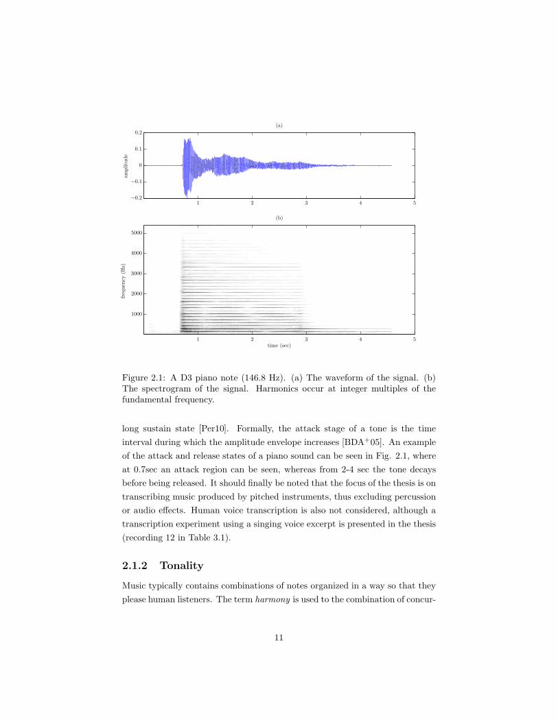
frequency-related scale extending from low to high”. As an example, Fig. 2.1
shows the waveform and spectrogram of a D3 piano note. In the spectrogram,
the partials can be seen as occurring at integer multiples of the fundamental
frequency (in this case it is 146.8 Hz).
It should be noted however that sounds produced by musical instruments
are not strictly harmonic due to the very nature of the sources (e.g. a stiff
string produces an inharmonic sound [JVV08, AS05]). Thus, a common as-
sumption made for pitched instruments is that they are quasi-periodic. There
are also cases of pitched instruments where the produced sound is completely
inharmonic, where in practice the partials are not integer multiples of a funda-
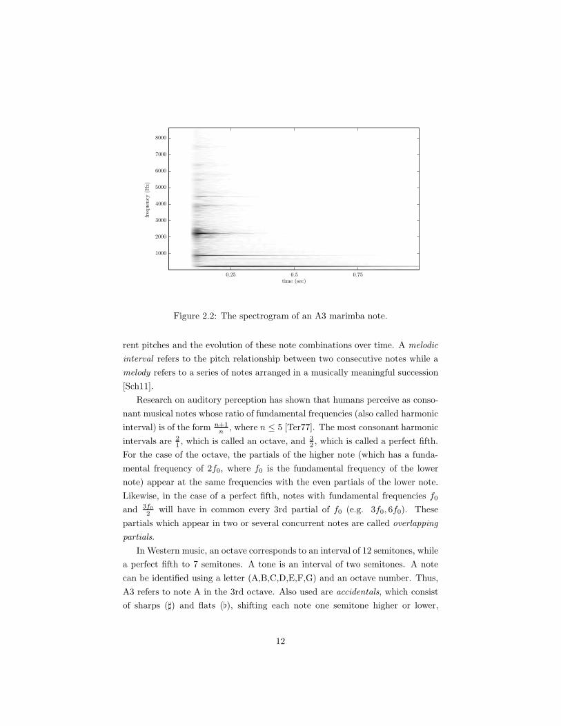
mental frequency, such as idiophones (e.g. marimba, vibraphone) [Per10]. An
example of an inharmonic sound is given in Fig. 2.2, where the spectrogram of
a Marimba A3 note can be seen.
Finally, a musical instrument might also exhibit frequency modulations such
as vibrato. In practice this means that the fundamental frequency changes
slightly. One such example of frequency modulations can be seen in Fig. 2.3,
where the spectrogram of a violin glissando followed by a vibrato is shown.
At around 3 sec, the vibrato occurs and the fundamental frequency (with its
corresponding partials) oscillates periodically over time. Whereas a vibrato
denotes oscillations in the fundamental frequency, a tremolo refers to a periodic
amplitude modulation, and can take place in woodwinds (e.g. flute) or in vocal
sounds [FR98].
Notes produced by musical instruments typically can be decomposed into
several temporal stages, denoting the temporal evolution of the sound. Pitched
percussive instruments (e.g. piano, guitar) have an attack stage, followed by
decay and release [BDA+05]. Bowed string or woodwind instruments have a
10
(b)
frequency
(Hz)
time (sec)
(a)amplitude
1 2 3 4 5
1 2 3 4 5
1000
2000
3000
4000
5000
−0.2
−0.1
0
0.1
0.2
Figure 2.1: A D3 piano note (146.8 Hz). (a) The waveform of the signal. (b)The spectrogram of the signal. Harmonics occur at integer multiples of thefundamental frequency.
long sustain state [Per10]. Formally, the attack stage of a tone is the time
interval during which the amplitude envelope increases [BDA+05]. An example
of the attack and release states of a piano sound can be seen in Fig. 2.1, where
at 0.7sec an attack region can be seen, whereas from 2-4 sec the tone decays
before being released. It should finally be noted that the focus of the thesis is on
transcribing music produced by pitched instruments, thus excluding percussion
or audio effects. Human voice transcription is also not considered, although a
transcription experiment using a singing voice excerpt is presented in the thesis
(recording 12 in Table 3.1).
2.1.2 Tonality
Music typically contains combinations of notes organized in a way so that they
please human listeners. The term harmony is used to the combination of concur-
11
frequency
(Hz)
time (sec)0.25 0.5 0.75
1000
2000
3000
4000
5000
6000
7000
8000
Figure 2.2: The spectrogram of an A3 marimba note.
rent pitches and the evolution of these note combinations over time. A melodic
interval refers to the pitch relationship between two consecutive notes while a
melody refers to a series of notes arranged in a musically meaningful succession
[Sch11].
Research on auditory perception has shown that humans perceive as conso-
nant musical notes whose ratio of fundamental frequencies (also called harmonic
interval) is of the form n+1n , where n ≤ 5 [Ter77]. The most consonant harmonic
intervals are 21 , which is called an octave, and 3
2 , which is called a perfect fifth.
For the case of the octave, the partials of the higher note (which has a funda-
mental frequency of 2f0, where f0 is the fundamental frequency of the lower
note) appear at the same frequencies with the even partials of the lower note.
Likewise, in the case of a perfect fifth, notes with fundamental frequencies f0
and 3f02 will have in common every 3rd partial of f0 (e.g. 3f0, 6f0). These
partials which appear in two or several concurrent notes are called overlapping
partials.
In Western music, an octave corresponds to an interval of 12 semitones, while
a perfect fifth to 7 semitones. A tone is an interval of two semitones. A note
can be identified using a letter (A,B,C,D,E,F,G) and an octave number. Thus,
A3 refers to note A in the 3rd octave. Also used are accidentals, which consist
of sharps (♯) and flats (), shifting each note one semitone higher or lower,
12
frequency
(Hz)
time (sec)1 2 3 4 5
1000
2000
3000
4000
5000
6000
7000
8000
Figure 2.3: The spectrogram of a violin glissando. A vibrato can be seen aroundthe 3 sec marker.
respectively. Although a succession of 7 octaves should result to the same note
as a succession of 12 fifths, the ratio (32 )12 : 27 is approximately 1.0136, which
is called a Pythagorean comma. Thus, some of the fifth intervals need to be
adjusted accordingly. Temperament refers to the various methods of adjusting
some or all of the fifth intervals (octaves are always kept pure) with the aim
of reducing the dissonance in the most commonly used intervals in a piece of
music [Bar51, Ver09].
One way of representing temperament is by the distribution of the Pythagorean
comma around the cycle of fifths, as seen in Fig 2.4. The most common tem-
perament is equal temperament, where each semitone is equal to one twelfth of
an octave. Thus, all fifths are diminished by 112 of a comma relative to the pure
ratio of 32 . Typically, equal temperament is tuned using note A4 as a reference
note with a fundamental frequency of 440 Hz.
A scale is a sequence of notes in ascending order which forms a perceptually
natural set [HM03]. The major scale follows the following pattern with respect
to semitones: 2-2-1-2-2-2-1. An example of a C major scale using Western
notation can be seen in Fig. 2.5. The natural minor scale has the pattern 2-1-2-
2-1-2-2 and the harmonic minor scale has the pattern 2-1-2-2-1-3-1. The key of
13

6
1
6
1
6
1
6
1
6
1
6
1
6
5
6
1
6
1
6
1
6
1
6
1
F
Bb
Eb
Ab
DbF#
B
E
A
D
GC
Sixth Comma Meantone
5
1
5
1
5
1
5
1
5
1
F
Bb
Eb
G#
C#F#
B
E
A
D
GC
Fifth Comma
Figure 2.4: Circle of fifths representation for the ‘Sixth comma meantone’ and‘Fifth comma’ temperaments. The deviation of each fifth from a pure fifth(the lighter cycle) is represented by the positions of the darker segments Thefractions specify the distribution of the comma between the fifths (if omittedthe fifth is pure). Fig. from [DTB11].
Figure 2.5: A C major scale, starting from C4 and finishing at C5.
a section of music is the scale which best fits the notes present. Using Western
harmony rules, a set of concurrent notes which sound pleasant to most people is
defined as a chord. A simple chord is the major triad (i.e. a three-note chord),
which in equal temperament has a fundamental frequency ratio of 4:5:6. The
consonance stems from the fact that these notes share many partials.
2.1.3 Rhythm
Rhythm describes the timing relationships between musical events within a piece
[CM60]. A main rhythmic concept is the metrical structure, which consists of
pulse sensations at different levels. Klapuri et al. [KEA06] consider three levels,
namely the tactus, tatum, and measure.
The tatum is the lowest level, considering the shortest durational values
which are commonly encountered in a piece. The tactus level consists of beats,
which are basic time units referring to the individual elements that make up a
14
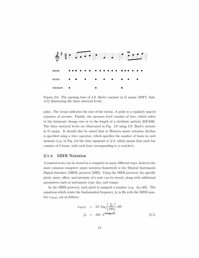
tatum
tactus
measure
Figure 2.6: The opening bars of J.S. Bach’s menuet in G major (BWV Anh.114) illustrating the three metrical levels.
pulse. The tempo indicates the rate of the tactus. A pulse is a regularly spaced
sequence of accents. Finally, the measure level consists of bars, which refers
to the harmonic change rate or to the length of a rhythmic pattern [KEA06].
The three metrical levels are illustrated in Fig. 2.6 using J.S. Bach’s menuet
in G major. It should also be noted that in Western music notation rhythm
is specified using a time signature, which specifies the number of beats in each
measure (e.g. in Fig. 2.6 the time signature is 3/4, which means that each bar
consists of 3 beats, with each beat corresponding to a crotchet).
2.1.4 MIDI Notation
A musical score can be stored in a computer in many different ways, however the
most common computer music notation framework is the Musical Instrument
Digital Interface (MIDI) protocol [MID]. Using the MIDI protocol, the specific
pitch, onset, offset, and intensity of a note can be stored, along with additional
parameters such as instrument type, key, and tempo.
In the MIDI protocol, each pitch is assigned a number (e.g. A3=69). The
equations which relate the fundamental frequency f0 in Hz with the MIDI num-
ber nMIDI are as follows:
nMIDI = 12 · log2
[f0440
]+69
f0 = 440 · 2nMIDI−69
12 (2.1)
15
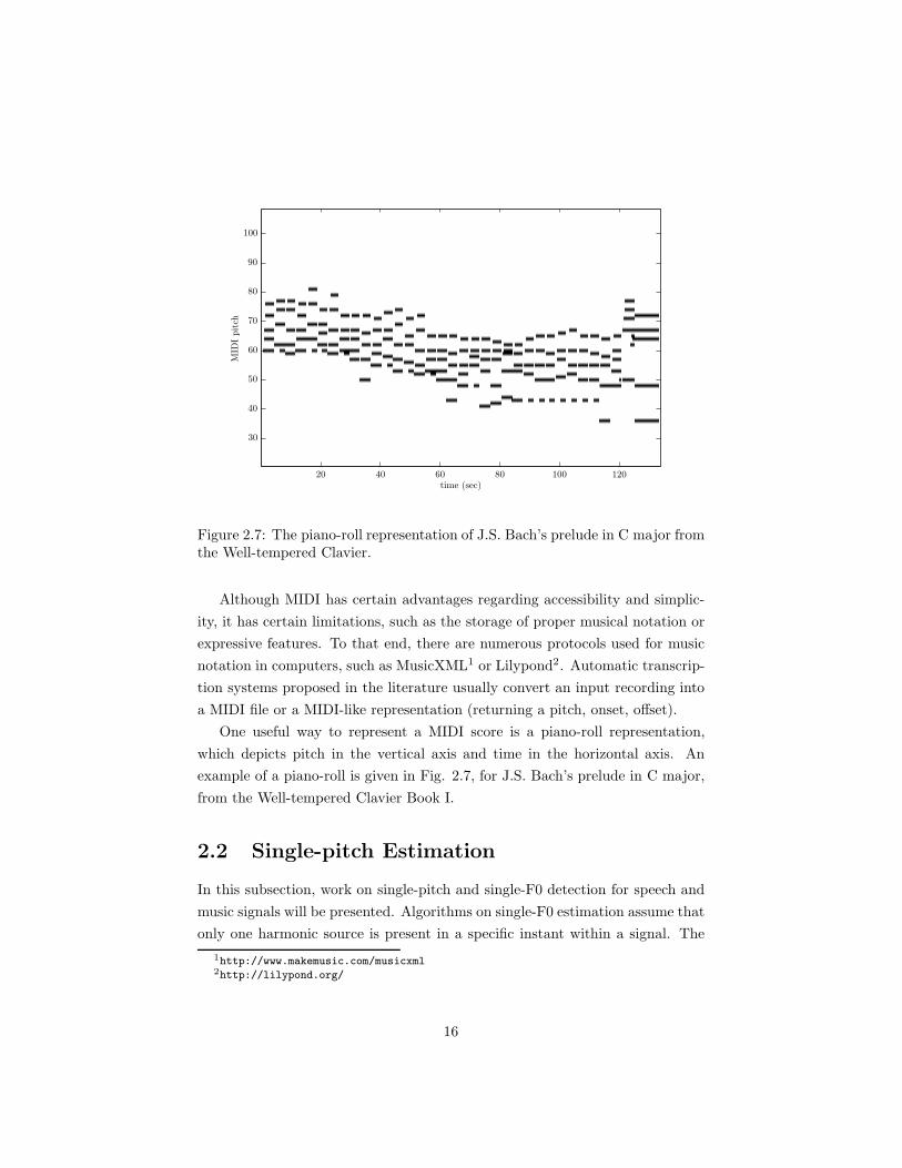
time (sec)
MID
Ipitch
20 40 60 80 100 120
30
40
50
60
70
80
90
100
Figure 2.7: The piano-roll representation of J.S. Bach’s prelude in C major fromthe Well-tempered Clavier.
Although MIDI has certain advantages regarding accessibility and simplic-
ity, it has certain limitations, such as the storage of proper musical notation or
expressive features. To that end, there are numerous protocols used for music
notation in computers, such as MusicXML1 or Lilypond2. Automatic transcrip-
tion systems proposed in the literature usually convert an input recording into
a MIDI file or a MIDI-like representation (returning a pitch, onset, offset).
One useful way to represent a MIDI score is a piano-roll representation,
which depicts pitch in the vertical axis and time in the horizontal axis. An
example of a piano-roll is given in Fig. 2.7, for J.S. Bach’s prelude in C major,
from the Well-tempered Clavier Book I.
2.2 Single-pitch Estimation
In this subsection, work on single-pitch and single-F0 detection for speech and
music signals will be presented. Algorithms on single-F0 estimation assume that
only one harmonic source is present in a specific instant within a signal. The
1http://www.makemusic.com/musicxml2http://lilypond.org/
16

Frequency (Hz)
Magnitude(dB)
0 1000 2000 3000 4000 5000 6000 7000 8000−90
−80
−70
−60
−50
−40
−30
−20
−10
0
Figure 2.8: The spectrum of a C4 piano note (sample from MAPS database[EBD10]).
single-F0 estimation problem is largely considered to be solved in the literature,
and a review on related methods can be found in [dC06]. In order to describe
single-F0 estimation methods we will use the same categorization, i.e. separate
approaches into spectral, temporal and spectrotemporal ones.
2.2.1 Spectral Methods
As mentioned in Section 2.1.1, the partials of a harmonic sound occur at integer
multiples of the fundamental frequency of that sound. Thus, a decision on
the pitch of a sound can be made by studying its spectrum. In Fig. 2.8 the
spectrum of a C4 piano note is shown, where the regular spacing of harmonics
can be observed.
The autocorrelation function can be used for detecting repetitive patterns
in signals, since the maximum of the autocorrelation function for a harmonic
spectrum corresponds to its fundamental frequency. Lahat et al. in [LNK87]
propose a method for pitch detection which is based on flattening the spectrum
of the signal and estimating the fundamental frequency from autocorrelation
functions. A subsequent smoothing procedure using median filtering is also
applied in order to further improve pitch detection accuracy.
In [Bro92], Brown computes the constant-Q spectrum [BP92] of an input
sound, resulting in a log-frequency representation. Pitch is subsequently de-
tected by computing the cross-correlation between the log-frequency spectrum
17

log-frequency index
CQT
Magnitude
0 100 200 300 400 500 6000
0.5
1
1.5
2
2.5
Figure 2.9: The constant-Q transform spectrum of a C4 piano note (samplefrom MAPS database [EBD10]). The lowest bin corresponds to 27.5 Hz and thefrequency resolution is 60 bins/octave.
and an ideal spectral pattern, which consists of ones placed at the positions
of harmonic partials. The maximum of the cross-correlation function indicates
the pitch for the specific time frame. The advantage of using a harmonic pat-
tern in log-frequency stems from the fact that the spacing between harmonics is
constant for all pitches, compared to a linear frequency representation (e.g. the
short-time Fourier transform). An example of a constant-Q transform spectrum
of a C4 piano note (the same as in Fig. 2.8) can be seen in Fig. 2.9.
Doval and Rodet [DR93] proposed a maximum likelihood (ML) approach for
fundamental frequency estimation which is based on a representation of an input
spectrum as a set of sinusoidal partials. To better estimate the f0 afterwards,
a tracking step using hidden Markov models (HMMs) is also proposed.
Another subset of single-pitch detection methods uses cepstral analysis. The
cepstrum is defined as the inverse Fourier transform of the logarithm of a signal
spectrum. Noll in [Nol67] proposed using the cepstrum for pitch estimation,
since peaks in the cepstrum indicate the fundamental period of a signal.
Finally, Kawahara et al. [KdCP98] proposed a spectrum-based F0 estimation
algorithm called “TEMPO”, which measures the instantaneous frequency at the
output of a filterbank.
18
2.2.2 Temporal Methods
The most basic approach for time domain-based single-pitch detection is the
use of the autocorrelation function using the input waveform [Rab77]. The
autocorrelation function is defined as:
ACF [ν] =1
N
N−ν−1∑
n=0
x[n]x[n + ν] (2.2)
where x[n] is the input waveform,N is the length of the waveform, and ν denotes
the time lag. For a periodic waveform, the first major peak in the autocorre-
lation function indicates the fundamental period of the waveform. However it
should be noted that peaks also occur at multiples of the period (also called
subharmonic errors). Another advantage of the autocorrelation function is that
it can be efficiently implemented using the discrete Fourier transform (DFT).
Several variants and extensions of the autocorrelation function have been
proposed in the literature, such as the average magnitude difference function
[RSC+74], which computes the city-block distance between a signal chunk and
another chunk shifted by ν. Another variant is the squared-difference function
[dC98], which replaced the city-block distance with the Euclidean distance:
SDF [ν] =1
N
N−ν−1∑
n=0
(x[n]− x[n+ ν])2 (2.3)
A normalized form of the squared-difference function was proposed by de
Cheveigne and Kawahara for the YIN pitch estimation algorithm [dCK02]. The
main improvement is that the proposed function avoids any spurious peaks near
zero lag, thus avoiding any harmonic errors. YIN has been shown to outperform
several pitch detection algorithms [dCK02] and is generally considered robust
and reliable for fundamental frequency estimation [dC06, Kla04b, Yeh08, Per10,
KD06].
2.2.3 Spectrotemporal Methods
It has been noted that spectrum-based pitch estimation methods have a ten-
dency to introduce errors which appear in integer multiples of the fundamental
frequency (harmonic errors), while time-based pitch estimation methods typ-
ically exhibit errors at submultiples of the f0 (subharmonic errors) [Kla03].
Thus, it has been argued that a tradeoff between spectral and temporal meth-
19

ACF
ACF
ACF
SACF+
HWR, Compression
HWR, Compression
HWR, Compression
AudioA
udito
ryFi
lterb
ank
b
b
b
b
b
b
Figure 2.10: Pitch detection using the unitary model of [MO97]. HWR refers tohalf-wave rectification, ACF refers to the autocorrelation function, and SACFto the summary autocorrelation function.
ods [dC06] could potentially improve upon pitch estimation accuracy.
Such a tradeoff can be formulated by splitting the input signal using a fil-
terbank, where each channel gives emphasis to a range of frequencies. Such a
filterbank is the unitary model by Meddis and Hewitt [MH92] which was utilized
by the same authors for pitch detection [MO97]. This model has links to human
auditory models. The unitary model consists of the following steps:
1. The input signal is passed into a logarithmically-spaced filterbank.
2. The output of each filter is half-wave rectified.
3. Compression and lowpass filtering is performed to each channel.
the output of the model can be used for pitch detection by computing the auto-
correlation for each channel and summing the results (summary autocorrelation
function). A diagram showing the pitch detection procedure using the unitary
model can be seen in Fig. 2.10. It should be noted however that harmonic
errors might be introduced by the half-wave rectification [Kla04b]. A similar
pitch detection model based on human perception theory which computes the
autocorrelation for each channel was also proposed by Slaney and Lyon [SL90].
2.3 Multi-pitch Estimation and Polyphonic Mu-
sic Transcription
In the polyphonic music transcription problem, we are interested in detecting
notes which might occur concurrently and could be produced by several instru-
20
ment sources. The core problem for creating a system for polyphonic music tran-
scription is thus multi-pitch estimation. For an overview on polyphonic tran-
scription approaches, the reader is referred to [KD06], while in [dC06] a review of
multiple-F0 estimation systems is given. A more recent overview on multi-pitch
estimation and polyphonic music transcription is given in [MEKR11].
As far as the categorization of the proposed methods is concerned, in [dC06]
multiple-F0 estimation methods are organized into three groups: temporal,
spectral, and spectrotemporal methods. However, the majority of multiple-F0
estimation methods employ a variant of a spectral method; even the system by
Tolonen [TK00] which depends on the summary autocorrelation function uses
the FFT for computational efficiency. Thus, in this section, two different clas-
sifications of polyphonic music transcription approaches will be made; firstly,
according to the time-frequency representation used and secondly according to
various techniques or models employed for multi-pitch detection.
In Table 2.1, approaches for multi-pitch detection and polyphonic music
transcription are organized according to the time-frequency representation em-
ployed. It can be clearly seen that most approaches use the short-time Fourier
transform (STFT) as a front-end, while a number of approaches use filter-
bank methods, such as the equivalent rectangular bandwidth (ERB) gamma-
tone filterbank, the constant-Q transform (CQT) [Bro91], the wavelet transform
[Chu92], and the resonator time-frequency image [Zho06]. The gammatone fil-
terbank with ERB channels is part of the unitary pitch perception model of
Meddis and Hewitt and its refinement by Meddis and O’Mard [MH92, MO97],
which compresses the dynamic level of each band, performs a non-linear pro-
cessing such as half-wave rectification, and performs low-pass filtering. Another
time-frequency representation that was proposed is specmurt [SKT+08], which
is produced by the inverse Fourier transform of a log-frequency spectrum.
Another categorization was proposed by Yeh in [Yeh08], separating systems
according to their estimation type as joint or iterative. The iterative estimation
approach extracts the most prominent pitch in each iteration, until no addi-
tional F0s can be estimated. Generally, iterative estimation models tend to
accumulate errors at each iteration step, but are computationally inexpensive.
In the contrary, joint estimation methods evaluate F0 combinations, leading to
more accurate estimates but with increased computational cost. However, re-
cent developments in the automatic music transcription field show that the vast
majority of proposed approaches now falls within the ‘joint’ category.
Thus, the classification that will be presented in this thesis organises auto-
21
Time-Frequency Representation Citation
Short-Time Fourier Transform [Abd02, AP04, AP06, BJ05, BED09a, BBJT04, BBFT10, BBST11][BKTB12, Bel03, BDS06, BMS00, BBR07, BD04, BS12, Bro06]
[BG10, BG11, CLLY07, OCR+08, OCR+09b, OCR+09a][OCQR10, OVC+11, CKB03, Cem04, CKB06, CSY+08]
[CJAJ04, CJJ06, CJJ07, CSJJ07, CSJJ08, Con06, DG03, DGI06][DCL10, Dix00, DR93, DZZS07, DHP09, DHP10, DPZ10][DDR11, EBD07, EBD08, EBD10, FHAB10, FK11, FCC05]
[Fon08, FF09, GBHL09, GS07a, GD02, GE09][GE10, GE11, Gro08, GS07a, Joh03, Kla01, Kla03, Kla04b, Kla06][Kla09a, Kla09b, KT11, LYLC10, LYC11, LYC12, LW07, LWB06]
[Lu06, MSH08, NRK+10, NRK+11, NLRK+11][NNLS11, NR07, Nie08, OKS12, OP11, ONP12]
[OS03, OBBC10, BQ07, QRC+10, CRV+10, PLG07][PCG10, PG11, Pee06, PI08, Per10, PI04][PI05, PI07, PI08, Per10, PI12, PAB+02]
[PEE+07, PE07a, PE07b, QCR+08, QCR+09][QCRO09, QRC+10, CRV+10, CQRSVC+10, ROS09a][ROS09b, RVBS10, Rap02, RFdVF08, RFF11, SM06]
[SC10, SC11, SB03, Sma11, Sun00, TL05, VK02][YSWJ10, WL06, Wel04, WS05]
[Yeh08, YR04, YRR05, YRR10, YSWS05, ZCJM10]ERB Filterbank [BBV09, BBV10, KT99, Kla04b, Kla05, Kla08, RK05, Ryy08]
[RK08, TK00, VR04, VBB07, VBB08, VBB10, ZLLX08]Constant-Q Transform [Bro92, CJ02, CPT09, CTS11, FBR11, KDK12]
[Mar12, MS09, ROS07, Sma09, Wag03, WVR+11b, WVR+11a]Wavelet Transform [FCC05, KNS04, KNS07, MKT+07, NEOS09]
[PHC06, SIOO12, WRK+10, YG10, YG12a]Constant-Q Bispectral Analysis [ANP11, NPA09]Resonator Time-Frequency Image [ZR07, ZR08, ZRMZ09, Zho06, BD10b, BD10a]
Multirate Filterbank [CQ98, Got00, Got04]Reassignment Spectrum [HM03, Hai03, Pee06]Modulation Spectrum [CDW07]
Matching Pursuit Decomposition [Der06]Multiresolution Fourier Transform [PGSMR12, KCZ09, Dre11]
Adaptive Oscillator Networks [Mar04]Modified Discrete Cosine Transform [SC09]
Specmurt [SKT+08]High-resolution spectrum [BLW07]
Quasi-Periodic Signal Extraction [TS09]
Table 2.1: Multiple-F0 estimation approaches organized according to the time-frequency representation employed.
matic music transcription systems according to the core techniques or models
employed for multi-pitch detection, as can be seen in Table 2.2. The majority
of these systems employ signal processing techniques, usually for audio feature
extraction, without resorting to any supervised or unsupervised learning pro-
cedures or classifiers for pitch estimation. Several approaches for note tracking
have been proposed using spectrogram factorisation techniques, most notably
non-negative matrix factorisation (NMF) [LS99]. NMF is a subspace analysis
method able to decompose an input time-frequency representation into a basis
matrix containing spectral templates for each component and a component ac-
tivity matrix over time. Maximum likelihood (ML) approaches, usually employ-
22

ing the expectation-maximization (EM) algorithm [DLR77, SS04], have been
also proposed in order to estimate the spectral envelope of candidate pitches
or to estimate the likelihood of a set of pitch candidates. Other probabilis-
tic methods include Bayesian models and networks, employing Markov Chain
Monte Carlo (MCMC) methods for reducing the computational cost. Hidden
Markov models (HMMs) [Rab89] are frequently used in a postprocessing stage
for note tracking, due to the sequential structure offered by the models. Su-
pervised training methods for multiple F0 estimation include support vector
machines (SVMs) [CST00], artificial neural networks, and Gaussian mixture
models (GMMs). Sparse decomposition techniques are also utilised, such as
the K-SVD algorithm [AEB05], non-negative sparse coding, and multiple signal
classification (MUSIC) [Sch86]. Least squares (LS) and alternating least squares
(ALS) models have also been proposed. Finally, probabilistic latent component
analysis (PLCA) [Sma04a] is a probabilistic variant of NMF which is also used
in spectrogram factorization models for automatic transcription.
2.3.1 Signal Processing Methods
Most multiple-F0 estimation and note tracking systems employ methods derived
from signal processing; a specific model is not employed, and notes are detected
using audio features derived from the input time-frequency representation either
in a joint or in an iterative fashion. Typically, multiple-F0 estimation occurs
using a pitch salience function (also called pitch strength function) or a pitch
candidate set score function [Kla06, PI08, YRR10]. In the following, signal
processing-based methods related to the current work will be presented in detail.
In [Kla03], Klapuri proposed an iterative spectral subtraction method with
polyphony inference, based on the principle that the envelope of harmonic
sounds tends to be smooth. A magnitude-warped power spectrum is used as
a data representation and a moving average filter is employed for noise sup-
pression. The predominant pitch is estimated using a bandwise pitch salience
function, which is able to handle inharmonicity [FR98, BQGB04, AS05]. After-
wards, the spectrum of the detected sound is estimated and smoothed before it
is subtracted from the input signal spectrum. A polyphony inference method
stops the iteration. A diagram showing the iterative spectral subtraction sys-
tem of [Kla03] can be seen in Fig. 2.11. This method was expanded in [Kla08],
where a variant of the unitary pitch model of [MO97] is used as a front-end,
and the summary autocorrelation function is used for detecting the predomi-
23

Technique Citation
Signal Processing Techniques [ANP11, BBJT04, BBFT10, BBST11, BKTB12, BLW07, Bro06, Bro92][CLLY07, OCR+08, OCR+09b, OCR+09a, Dix00, Dre11]
[DZZS07, FHAB10, CQ98, FK11, Gro08, PGSMR12, HM03][Hai03, Joh03, KT99, Kla01, Kla03]
[Kla04b, Kla05, Kla06, Kla08, LRPI07, LWB06, NPA09][BQ07, PHC06, PI07, PI08, Per10, PI12]
[QCR+09, QCRO09, CQRSVC+10, SKT+08, SC09, TK00][Wag03, WZ08, YSWJ10, WL06, WS05, YR04, YRR05]
[Yeh08, YRR10, YSWS05, ZLLX08, Zho06, ZR07, ZR08, ZRMZ09]Maximum Likelihood [BED09a, DHP09, DPZ10, EBD07, EBD08, EBD10, FHAB10, Got00]
[Got04, KNS04, KNS07, KT11, MKT+07, NEOS09, NR07][Pee06, SIOO12, WRK+10, WVR+11b, WVR+11a, YG10, YG12b, YG12a]
Spectrogram Factorization [BBR07, BBV09, BBV10, OVC+11, Con06, CDW07, CTS11][DCL10, DDR11, FBR11, GE09, GE10, GE11, HBD10, HBD11a]
[HBD11b, KDK12, Mar12, MS09, NRK+10, NRK+11, NLRK+11, Nie08][OKS12, ROS07, ROS09a, ROS09b, SM06, SB03, Sma04b]
[Sma09, Sma11, VBB07, VBB08, VBB10, VMR08]Hidden Markov Models [BJ05, CSY+08, EP06, EBD08, EBD10, LW07, OS03, PE07a, PE07b]
[QRC+10, CRV+10, Rap02, Ryy08, RK05, SC10, SC11, VR04]Sparse Decomposition [Abd02, AP04, AP06, BBR07, BD04, OCQR10, CK11, Der06, GB03]
[LYLC10, LYC11, LYC12, MSH08, OP11, ONP12, PAB+02, QCR+08]Multiple Signal Classification [CJAJ04, CJJ06, CSJJ07, CJJ07, CSJJ08, ZCJM10]Support Vector Machines [CJ02, CPT09, EP06, GBHL09, PE07a, PE07b, Zho06]
Dynamic Bayesian Network [CKB03, Cem04, CKB06, KNKT98, ROS09b, RVBS10]Neural Networks [BS12, GS07a, Mar04, NNLS11, OBBC10, PI04, PI05]
Bayesian Model + MCMC [BG10, BG11, DGI06, GD02, PLG07, PCG10, PG11, TL05]Genetic Algorithms [Fon08, FF09, Lu06, RFdVF08, RFF11]Blackboard System [BMS00, BDS06, Bel03, McK03]
Subspace Analysis Methods [FCC05, VR04, Wel04]Temporal Additive Model [BDS06, Bel03]Gaussian Mixture Models [Kla09a, Mar07]
Least Squares [Kla09b, KCZ09]
Table 2.2: Multiple-F0 and note tracking techniques organised according to theemployed technique.
nant pitch. In [RK05] the system of [Kla03] was combined with a musicological
model for estimating musical key and note transition probabilities. Note events
are described using 3-state hidden Markov models (HMMs), which denote the
attack, sustain, and noise/silence state of each sound. Also incorporated was
information from an onset detection function. The system of [RK05] was also
publicly evaluated in the MIREX 2008 multiple-F0 estimation and note track-
ing task [MIR] where competitive results were reported. Also, in [BKTB12],
the system of [Kla08] was utilised for transcribing guitar recordings and also
for extracting fingering configurations. An HMM was incorporated in order to
model different fingering configurations, which was combined with the salience
function of [Kla08]. Fingering transitions are controlled using a musicological
model which was trained on guitar chord sequences.
Yeh et al. [YRR10] present a joint pitch estimation algorithm based on a
24

Figure 2.11: The iterative spectral subtraction system of Klapuri (figure from[Kla03]).
pitch candidate set score function. The front-end of the algorithm consists of a
short-time Fourier transform (STFT) computation followed by an adaptive noise
level estimation method based on the assumption that the noise amplitude fol-
lows a Rayleigh distribution. Given a set of pitch candidates, the overlapping
partials are detected and smoothed according to the spectral smoothness prin-
ciple [Kla03]. The weighted score function for the pitch candidate set consists of
4 features: harmonicity, mean bandwidth, spectral centroid, and synchronicity.
A polyphony inference mechanism based on the score function increase selects
the optimal pitch candidate set. The automatic transcription methods proposed
by Yeh et al. [YRR05, Yeh08, YRR10] have been publicly evaluated in several
MIREX competitions [MIR], where they rank first or amongst the first ones.
Pertusa and Inesta [PI08, Per10, PI12] propose a computationally inexpen-
sive method similar to Yeh’s. The STFT of the input signal is computed, and
a simple pitch salience function is computed. For each possible combination in
the pitch candidate set, an overlapping partial treatment procedure is applied.
Each harmonic partial sequence (HPS) is further smoothed using a truncated
normalised Gaussian window, and a measure between the HPS and the smooth
HPS is computed, which indicates the salience of the pitch hypothesis. The
pitch candidate set with the greatest salience is selected for the specific time
frame. In a postprocessing stage, minimum duration pruning is applied in order
to eliminate local errors. In Fig. 2.12, an example of the Gaussian smoothing
of [PI08] is given, where the original HPS can be seen along with the smoothed
HPS.
Zhou et al. [ZRMZ09] proposed an iterative method for polyphonic pitch esti-
25

Smooth HPS
Original HPSPartialmagnitude
Partial Index0 1 2 3 4 5 6 7 8 9 10 11
0
0.2
0.4
0.6
0.8
1
Figure 2.12: Example of the Gaussian smoothing procedure of [PI08] for aharmonic partial sequence.
mation using a complex resonator filterbank as a front-end, called the resonator
time-frequency image (RTFI) [Zho06]. An example of the RTFI spectrum is
given in Fig. 2.13. A mid-level representation is computed, called the pitch
energy spectrum and pitch candidates are selected. Additional pitch candidates
are selected from the RTFI using harmonic component extraction. These candi-
dates are then eliminated in an iterative fashion using a set of rules based on fea-
tures of the HPS. These rules are based on the number of harmonic components
detected for each pitch and the spectral irregularity measure, which measures
the concentrated energy around possibly overlapped partials from harmonically-
related F0s. This method has been implemented as a real-time polyphonic mu-
sic transcription system and has also been evaluated in the MIREX framework
[MIR].
A mid-level representation along with a respective method for multi-pitch
estimation was proposed by Saito et al. in [SKT+08], by using the inverse
Fourier transform of the linear power spectrum with log-scale frequency, which
was called specmurt (an anagram of cepstrum). The input spectrum (generated
by a wavelet transform) is considered to be generated by a convolution of a
common harmonic structure with a pitch indicator function. The deconvolution
of the spectrum by the harmonic pattern results in the estimated pitch indicator
function, which can be achieved through the concept of specmurt analysis. This
26
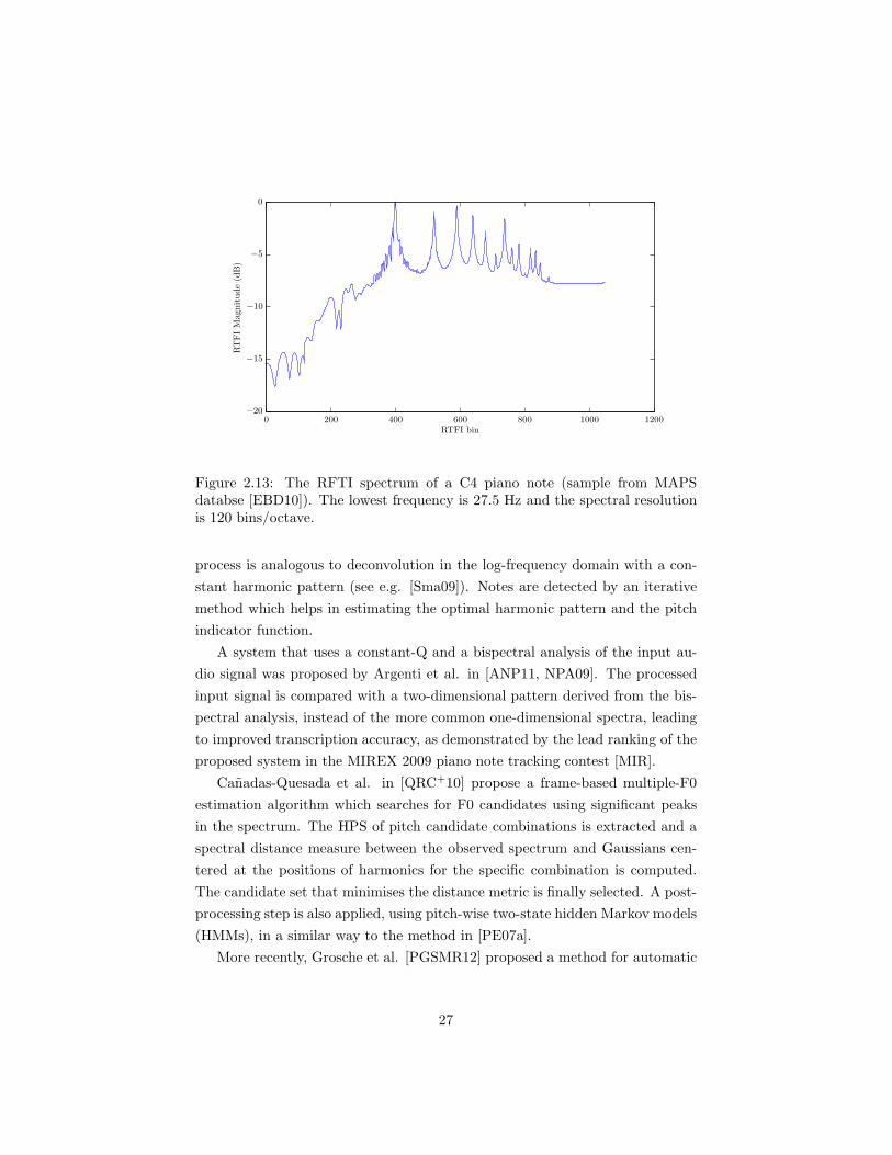
RTFI bin
RTFIMagnitude(dB)
0 200 400 600 800 1000 1200−20
−15
−10
−5
0
Figure 2.13: The RFTI spectrum of a C4 piano note (sample from MAPSdatabse [EBD10]). The lowest frequency is 27.5 Hz and the spectral resolutionis 120 bins/octave.
process is analogous to deconvolution in the log-frequency domain with a con-
stant harmonic pattern (see e.g. [Sma09]). Notes are detected by an iterative
method which helps in estimating the optimal harmonic pattern and the pitch
indicator function.
A system that uses a constant-Q and a bispectral analysis of the input au-
dio signal was proposed by Argenti et al. in [ANP11, NPA09]. The processed
input signal is compared with a two-dimensional pattern derived from the bis-
pectral analysis, instead of the more common one-dimensional spectra, leading
to improved transcription accuracy, as demonstrated by the lead ranking of the
proposed system in the MIREX 2009 piano note tracking contest [MIR].
Canadas-Quesada et al. in [QRC+10] propose a frame-based multiple-F0
estimation algorithm which searches for F0 candidates using significant peaks
in the spectrum. The HPS of pitch candidate combinations is extracted and a
spectral distance measure between the observed spectrum and Gaussians cen-
tered at the positions of harmonics for the specific combination is computed.
The candidate set that minimises the distance metric is finally selected. A post-
processing step is also applied, using pitch-wise two-state hidden Markov models
(HMMs), in a similar way to the method in [PE07a].
More recently, Grosche et al. [PGSMR12] proposed a method for automatic
27

transcription based on a mid-level representation derived from a multiresolu-
tion Fourier transform combined with an instantaneous frequency estimation.
The system also combines onset detection and tuning estimation for computing
frame-based estimates. Note events are afterwards detected using 2 HMMs per
pitch, one for the on state and one for the off state.
2.3.2 Statistical Modelling Methods
Many approaches in the literature formulate the multiple-F0 estimation problem
within a statistical framework. Given an observed frame v and a set C of
all possible fundamental frequency combinations, the frame-based multiple-F0
estimation problem can then be viewed as a maximum a posteriori (MAP)
estimation problem [EBD10]:
C = argmaxC∈C
P (C|v) (2.4)
where C is the estimated set of fundamental frequencies and P (·) denotes prob-
ability. If no prior information on the mixtures is specified, the problem can be
expressed as a maximum likelihood (ML) estimation problem using Bayes’ rule
[CKB06, DPZ10, EBD10]:
C = argmaxC∈C
P (v|C)P (C)
P (v)= argmax
C∈C
P (v|C) (2.5)
Goto in [Got00, Got04] proposed an algorithm for predominant-F0 estima-
tion of melody and bass line based on MAP estimation, called PreFEst. The
input time-frequency representation (which is in log-frequency and is computed
using instantaneous frequency estimation) is modelled using a weighted mixture
of adapted tone models, which exhibit a harmonic structure. In these tone mod-
els, a Gaussian is placed in the position of each harmonic over the log-frequency
axis. MAP estimation is performed using the expectation-maximization (EM)
algorithm. In order to track the melody and bass-line F0s over time, a multiple-
agent architecture is used, which selects the most stable F0 trajectory. An
example of the tone model used in [Got04] is given in Fig. 2.14.
A Bayesian harmonic model was proposed by Davy and Godsill in [DG03],
which models the spectrum as a sum of Gabor atoms with time-varying am-
plitudes with non-white residual noise, while inharmonicity is also considered.
The unknown model parameters are estimated using a Markov chain Monte
28

Magnitude
Log-frequency bin0 100 200 300 400 500 600
0
0.2
0.4
0.6
0.8
1
Figure 2.14: An example of the tone model of [Got04]. Each partial in thelog-frequency domain is modelled by a Gaussian probability density function(PDF). The log-frequency resolution is 120 bins/octave.
Carlo (MCMC) method. The model was expanded in [DGI06], also including
the extraction of dynamics, timbre, and instrument type.
An expansion of Goto’s method from [Got04] was proposed by Kameoka
et al. [KNS04, KNS07], called harmonic temporal structured clustering (HTC),
which jointly estimates multiple fundamental frequencies, onsets, offsets, and
dynamics. The input time-frequency representation is a wavelet spectrogram.
Partials are modelled using Gaussians placed in the positions of partials in the
log-frequency domain and the synchronous evolution of partials belonging to
the same source is modelled by Gaussian mixtures. Time-evolving partials from
the same source are then clustered. Model parameters are learned using the
EM algorithm. The HTC algorithm was also used for automatic transcription
in [MKT+07], where rhythm and tempo are also extracted using note duration
models with HMMs. A variant of the HTC algorithm was publicly evaluated for
the MIREX competition [NEOS09], where an iterative version of the algorithm
was used and penalty factors for the maximum number of active sources were
incorporated into the HTC likelihood.
The HTC algorithm was also utilised in [WRK+10] for instrument identifica-
tion in polyphonic music, where for each detected note event harmonic temporal
timbre features are computed and a support vector machine (SVM) classifier is
used for instrument identification. The HTC algorithm was further extended
by Wu et al. in [WVR+11a], where each note event is separated into an attack
and sustain state. For the attack states, an inharmonic model is used which
is characterised by a spectral envelope and a respective power. For the sustain
states, a harmonic model similar to [KNS07] is used. Instrument identification
29

is also performed using an SVM classifier, in a similar way to [WRK+10].
A maximum likelihood approach for multiple-F0 estimation which models
spectral peaks and non-peak regions was proposed by Duan et al. in [DHP09,
DPZ10]. The likelihood function of the model is composed of the peak region
likelihood (probability that a peak is detected in the spectrum given a pitch)
and the non-peak region likelihood (probability of not detecting any partials in a
non-peak region), which are complementary. An iterative greedy F0 estimation
procedure is proposed and priors are learned from monophonic and polyphonic
training data. Polyphony inference, in order to control the number of itera-
tions, is achieved by a threshold-based method using the likelihood function. A
post-processing stage is performed using neighboring frames. Experiments were
performed on the newly released Bach10 dataset3, which contains multi-track
recordings of Bach chorales. The methods in [DHP09, DPZ10] were also pub-
licly evaluated in the MIREX 2009 and 2010 contests and ranked second best
in the multiple-F0 estimation task.
Badeau et al. in [BED09a] proposed a maximum likelihood approach for
multiple-pitch estimation which performs successive single-pitch and spectral
envelope estimations. Inference is achieved using the expectation-maximization
(EM) algorithm. As a continuation of the work of [BED09a], Emiya et al. in
[EBD10] proposed a joint estimation method for piano notes using a likelihood
function which models the spectral envelope of overtones using a smooth au-
toregressive (AR) model and models the residual noise using a low-order moving
average (MA) model. The likelihood function is able to handle inharmonicity
and the amplitudes of overtones are considered to be generated by a complex
Gaussian random variable. The authors of [EBD10] also created a large database
for piano transcription called MAPS, which was used for experiments. MAPS
contains isolated notes and music pieces from synthesised and real pianos in
different recording setups.
Raczynski et al. in [RVBS10] developed a probabilistic model for multiple
pitch transcription based on dynamic Bayesian networks (DBNs) that takes
into account temporal dependencies between musical notes and between the
underlying chords, as well as the instantaneous dependencies between chords,
notes and the observed note saliences. In addition, a front-end for obtaining
initial note estimates was also used, which relied on the non-negative matrix
factorization (NMF) algorithm.
3http://music.cs.northwestern.edu
30
Peeling and Godsill [PCG10, PG11] proposed a likelihood function for multiple-
F0 estimation where for a given time frame, the occurrence of peaks in the fre-
quency domain is assumed to follow an inhomogeneous Poisson process. This
method was updated in [BG10, BG11], where in order to link detected pitches
between adjacent frames, a model is proposed using Bayesian filtering and in-
ference is achieved using the sequential MCMC algorithm. It should be noted
however that the proposed likelihood function takes only into account the posi-
tion of partials in f0 candidates and not their amplitudes.
An extension of the PreFEst algorithm in [Got04] was proposed in [YG10,
YG12a], where a statistical method called Infinite Latent Harmonic Allocation
(iLHA) was proposed for detecting multiple fundamental frequencies in poly-
phonic audio signals, eliminating the problem of fixed system parameters. The
proposed method assumes that the observed spectra are superpositions of a
stochastically-distributed unbounded (theoretically infinite) number of bases.
For inference, a modified version of the variational Bayes (VB) algorithm was
used. In [YG12b], the method of [YG12a] was also used for unsupervised mu-
sic understanding, where musicological models are also learned from the input
signals. Finally, the iLHA method was improved by Sakaue et al. [SIOO12],
where a corpus of overtone structures of musical instruments taken from a MIDI
synthesizer was used instead of the prior distributions of the original iLHA al-
gorithm.
Koretz and Tabrikian [KT11] proposed an iterative method for multi-pitch
estimation, which combines MAP and ML criteria. The predominant source
is expressed using a harmonic model while the remaining harmonic signals are
modelled as Gaussian interference sources. After estimating the predominant
source, it is removed from the spectrogram and the process is iterated, in a
similar manner to the spectral subtraction method of [Kla03]. It should also be
noted that the algorithm was also tested on speech signals in addition to music
signals.
2.3.3 Spectrogram Factorization Methods
A large subset of recent automatic music transcription approaches employ spec-
trogram factorization techniques. These techniques are mainly non-negative
matrix factorization (NMF) [LS99] and its probabilistic counterpart, proba-
bilistic latent component analysis (PLCA) [SRS06]. Both of these algorithms
will be presented in detail, since a large set of proposed automatic transcription
31

methods in this thesis are based on PLCA and NMF.
Non-negative Matrix Factorization
Subspace analysis seeks to find low dimensional structures of patterns within
high-dimensional spaces. Non-negative matrix factorization (NMF) [LS99] is
a subspace method able to obtain a parts-based representation of objects by
imposing non-negative constraints. In music signal analysis, it has been shown
to be useful in representing a spectrogram as a parts-based representation of
sources or notes [MEKR11], thus the use of the term spectrogram factorization.
NMF was first introduced as a tool for music transcription by Smaragdis
and Brown [SB03]. In NMF, an input matrix V ∈ RΩ×T+ can be decomposed
as:
V ≈WH (2.6)
where H ∈ RZ×T+ is the atom activity matrix across T and W ∈ R
Ω×Z+ is the
atom basis matrix. In (2.6), Z is chosen as min(Ω, T ), as to reduce the data
dimension. In order to achieve the factorization, a distance measure between
the input V and the reconstruction WH is employed, with the most common
being the Kullback-Leibler (KL) divergence or the Euclidean distance.
Thus, in the case of an input magnitude or power spectrogram V, H is the
atom activity matrix across time and W is the atom spectral basis matrix. In
that case also, t = 1, . . . , T is the time index and ω = 1, . . . ,Ω is the frequency
bin index, while z = 1, . . . , Z is the atom/component index. An example of
the NMF algorithm applied to a music signal is shown in Fig. 2.15, where the
spectrogram of the opening bars of J.S. Bach’s English Suite No. 5 is decomposed
into note atoms W and atom activations H.
In addition to [SB03], the standard NMF algorithm was also employed by
Bertin et al. in [BBR07] where an additional post-processing step was presented,
in order to associate atoms with pitch classes and to accurately detect note
onsets and offsets.
Several extensions of NMF have been used for solving the automatic tran-
scription problem. In [Con06], Cont has added sparseness constraints into the
NMF update rules, in an effort to find meaningful transcriptions using a min-
imum number of non-zero elements in H. In order to formulate the sparse-
ness constraint into the NMF cost function, the lǫ norm is employed, which
is approximated by the tanh function. An extension of the work in [Con06]
was proposed in [CDW07], where the input time-frequency representation was
32
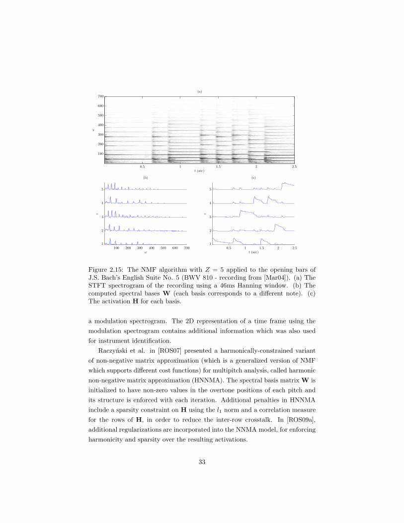
z
t (sec)
(c)
z
ω
(b)
ω
t (sec)
(a)
0.5 1 1.5 2 2.5100 200 300 400 500 600 700
0.5 1 1.5 2 2.5
1
2
3
4
5
1
2
3
4
5
100
200
300
400
500
600
700
Figure 2.15: The NMF algorithm with Z = 5 applied to the opening bars ofJ.S. Bach’s English Suite No. 5 (BWV 810 - recording from [Mar04]). (a) TheSTFT spectrogram of the recording using a 46ms Hanning window. (b) Thecomputed spectral bases W (each basis corresponds to a different note). (c)The activation H for each basis.
a modulation spectrogram. The 2D representation of a time frame using the
modulation spectrogram contains additional information which was also used
for instrument identification.
Raczynski et al. in [ROS07] presented a harmonically-constrained variant
of non-negative matrix approximation (which is a generalized version of NMF
which supports different cost functions) for multipitch analysis, called harmonic
non-negative matrix approximation (HNNMA). The spectral basis matrix W is
initialized to have non-zero values in the overtone positions of each pitch and
its structure is enforced with each iteration. Additional penalties in HNNMA
include a sparsity constraint on H using the l1 norm and a correlation measure
for the rows of H, in order to reduce the inter-row crosstalk. In [ROS09a],
additional regularizations are incorporated into the NNMA model, for enforcing
harmonicity and sparsity over the resulting activations.
33

Niedermayer in [Nie08] introduced a method aiming to incorporate prior
knowledge about the pitch dictionary into the NMF algorithm. His approach
was called non-negative matrix division, and it included a step for tone model
learning before using a modified version of the unconstrained NMF with Eu-
clidean distance in order to extract the transcription. As an input, the magnitude-
warped power spectrum of [Kla03] was used.
Vincent et al. [VBB07, VBB08] incorporated harmonicity constraints in the
NMF model, resulting in two algorithms; harmonic and inharmonic NMF. The
model additionally constrains each basis spectrum to be expressed as a weighted
sum of narrowband spectra, in order to preserve a smooth spectral envelope for
the resulting basis functions. The inharmonic version of the algorithm is also
able to support inharmonic spectra and tuning deviations. An ERB-scale time-
frequency representation is used as input and a threshold-based onset/offset
detection is performed in a post-processing step. The harmonic constraints and
the post-processing procedure for note identification and onset/offset detection
were further refined in [VBB10].
A model for automatic transcription of multiple-instrument recordings was
proposed in [GE09], which extends the NMF algorithm to incorporate con-
straints on the basis vectors. Instrument models are incorporated using a group-
ing of spectral bases, called eigeninstruments.
Bertin et al. [BBV09, BBV10] expanded upon the work of [VBB08], propos-
ing a Bayesian framework for NMF, which considers each pitch as a model of
Gaussian components in harmonic positions. Spectral smoothness constraints
are incorporated into the likelihood function and for parameter estimation the
space alternating generalized EM algorithm (SAGE) is employed. Temporal
smoothness of the detected notes is also enforced by using a Markov chain prior
structure.
Nakano et al. [NRK+10] propose an NMF algorithm with Markov-chained
basis for modelling the temporal evolution of music sounds. The goal of the
system is to learn the time-varying sound states of musical instruments, such
as attack, sustain, and decay, without any prior information. The proposed
method is linked to the Viterbi algorithm using Factorial HMMs [GJ97].
In [DCL10], the NMF algorithm with β-divergence is utilised for piano tran-
scription. β-divergence is a parametric family of distortion functions which can
be used in the NMF cost function to influence the NMF update rules for W
and H. Essentially, β = 0 equally penalizes a bad fit of factorization for small
and large coefficients while when β > 0, emphasis is given to components with
34

t (sec)
MID
Ipitch
(c)
MID
Ipitch
(b)
MID
Ipitch
(a)
0.4 0.8 1.2 1.6 2.0 2.4
0.4 0.8 1.2 1.6 2.0 2.4
0.4 0.8 1.2 1.6 2.0 2.4
40
50
60
70
80
90
40
50
60
70
80
90
40
50
60
70
80
90
Figure 2.16: The activation matrix of the NMF algorithm with β-divergenceapplied to the monophonic melody of Fig. 2.15. (a) β = 0 (b) β = 0.5 (c)β = 1.
greater energy. A tradeoff between an equal penalization and a penalization of
coefficients with high energy only has been shown to produce improved results
for harmonic sounds (which typically have a strong fundamental and weaker
harmonics). It should also be mentioned that the method of [DCL10] was pub-
licly evaluated in the MIREX contest, giving good results in the piano-only note
tracking task. An example of the use of parameter β for the transcription of
the opening bars of J.S. Bach’s English Suite No. 5 can be seen in Fig. 2.16.
Costantini et al. in [CTS11] employed a variant of the NMF algorithm with
sparsity constraints for the activation matrix, using the constant-Q transform
as a time-frequency representation. The system also incorporated an onset
detector for splitting the input spectrogram into segments.
35
Hennequin et al. [HBD10, HBD11a] proposed an NMF-based algorithm for
music signal analysis in order to model non-stationary note events. Since in a
tone each harmonic decays with a different rate, the proposed model extends the
NMF algorithm by including time-frequency activations based on autoregressive
moving average (ARMA) modeling.
Carabias-Orti et al. [OVC+11] proposed a spectrogram factorization tech-
nique for automatic transcription as well as for musical instrument identification
in polyphonic music. A harmonic comb-based excitation-filter model was incor-
porated into the NMF framework in order to model the excitation of different
musical instruments.
Durrieu et al. [DDR11] proposed a mid-level representation which com-
bines a source-filter model with the NMF algorithm in order to produce a pitch
track which also contains timbral information. This mid-level representation
was shown to be useful not only for multi-pitch detection, but also for melody
extraction and lead instrument/accompaniment separation.
Marolt [Mar12] proposed a system for automatically transcribing bell chim-
ing recordings using a modified version of the k-means algorithm for estimating
the number of bells in the recording and the NMF algorithm for estimating the
basis spectra of each bell. This system also incorporates an onset detector for
improving transcription performance.
Ochiai et al. [OKS12] propose an algorithm for multi-pitch detection and
beat structure analysis. The NMF objective function is constrained using in-
formation from the rhythmic structure of the recording, which helps improve
transcription accuracy in highly repetitive recordings.
Non-negative Matrix Deconvolution
Another variant of the NMF algorithm changes the model from a linear to
a convolutive one. Thus, two-dimensional bases can be learned from a time-
frequency representation, where the 2-D atoms are convolved with atom ac-
tivations. In [Sma04a, Sma04b], non-negative matrix deconvolution (NMD) is
proposed, whereV is considered to be the result of a convolution of time-varying
spectra with their activity matrices. The NMD model can be formulated as:
V ≈
T −1∑
τ=0
Wτ ·−→Hτ (2.7)
36
where Wτ ∈ RΩ×Z , H ∈ R
Z×T , and−→Hτ denotes shifting the columns of H by
τ spots to the right.
Schmidt and Mørup in [MS06, SM06] proposed an extension of NMD with
sparsity constraints, called sparse non-negative matrix factor 2-D deconvolution
(SNMF2D) for automatic transcription of polyphonic music. The method oper-
ates in the log-frequency domain, considering a constant shifted 2-D harmonic
structure as a basis. In this case, the l 12norm of H was used in order to control
the sparseness, while non-negativity constraints on Wτ and H are explicitly
enforced for each iteration. It should also be noted that in [CSS11], an alterna-
tive formulation of the NMD models is made, called probabilistic latent tensor
factorization (PLTF).
In [KDK12], a method for semi-automatic music transcription is proposed
which is based on a proposed model for shift-invariant NMD. The algorithm op-
erates in the log-frequency domain and extracts a different instrument spectrum
for each fundamental frequency under analysis. The term semi-automatic tran-
scription refers to the user providing prior information about the polyphonic
mixture or user transcribing some notes for each instrument in the mixture.
Probabilistic Latent Component Analysis
An alternative formulation of NMF was proposed by Smaragdis in [SRS06],
called probabilistic latent component analysis (PLCA). It can be viewed as a
probabilistic extension of the non-negative matrix factorization (NMF) algo-
rithm [LS99] using the Kullback-Leibler cost function, providing a framework
that is easy to generalize and interpret. PLCA can also offer a convenient way to
incorporate priors over the parameters and control the resulting decomposition,
for example using entropic priors [SRS08a]. In PLCA, the input spectrogram
Vω,t (ω denotes frequency, and t time), which must be scaled to have integer
entries, is modeled as the histogram of the draw of N independent random
variables (ωn, tn) which are distributed according to P (ω, t). P (ω, t) can be
expressed by the product of a spectral basis matrix and a component activity
matrix.
The asymmetric form of the PLCA model is expressed as:
Pt(ω) =∑
z
P (ω|z)Pt(z) (2.8)
where z is the component index, P (ω|z) is the spectral template that corre-
37
sponds to the z-th component, and Pt(z) is the activation of the z-th compo-
nent.
The generative model for PLCA as presented in [Sha07] is as follows:
1. Choose z according to Pt(z).
2. Choose ω according to P (ω|z).
3. Repeat the above steps Vt times (Vt =∑ω Vω,t).
In order to estimate the unknown parameters P (ω|z) and Pt(z), iterative
update rules are applied, using the Expectation-Maximization (EM) algorithm
[DLR77, SS04]. For the E-step, the a posteriori probability for the latent variable
is derived using Bayes’ theorem:
Pt(z|ω) =P (ω|z)Pt(z)∑z P (ω|z)Pt(z)
(2.9)
For the M-step, the expected complete data log-likelihood is maximised. The
expected log-likelihood is given by [Sha07]:
L = Ez|ω;Λ logP (ω, z) (2.10)
where ω, z represent the set of all observations for ω, z and Λ = P (ω|z), Pt(z).
The complete data likelihood P (ω, z) can be written as:
P (ω, z) =∏
j,t
Pt(zj)P (ωj |zj) (2.11)
where ωj , zj are the values of ω, z in their j-th draw. Thus, L can be written
as:
L =∑
j,t,z
P (z|ωj) logPt(z) +∑
j,t,z
P (z|ωj) logP (ωj|z) (2.12)
By introducing Lagrange multipliers in (2.12) and maximising with respect to
P (ω|z) and Pt(z) leads to the following M-step equations:
P (ω|z) =
∑t Vω,tPt(z|ω)∑ω,t Vω,tPt(z|ω)
(2.13)
Pt(z) =
∑ω Vω,tPt(z|ω)∑z,ω Vω,tPt(z|ω)
(2.14)
The update rules of (2.9)-(2.14) are guaranteed to converge to a local min-
38

t
(d)
ω
(c)
t
ω
(b)
t
ω
(a)
0 20 40 60 80 100 120200 400 600 800 1000
20 40 60 80 10020 40 60 80 100
0
50
100
150
0
0.2
0.4
0.6
0.8
1
200
400
600
800
1000
200
400
600
800
1000
Figure 2.17: (a) The log-frequency spectrogram P (ω, t) of a C4 piano note (b)Approximation of the spectrogram using PLCA with z = 1 component (c) Thespectral template P (ω|z) (d) The gain Pt(z).
imum. In Fig. 2.17, an example of the application of the PLCA method to a
log-frequency spectrogram of a piano note can be seen.
An extension of the asymmetric PLCA algorithm was used for multiple-
instrument transcription in [GE10, GE11], where a system was proposed which
supported multiple spectral templates for each pitch and instrument source.
The notion of eigeninstruments was again utilised (as in [GE09]), by modeling
the fixed spectral templates as a linear combination of basic instrument models
in a training step. The model was expressed as:
P (ω, t) = P (t)∑
s
∑
p
∑
z
P (ω|p, z, s)P (z|s, p, t)P (s|p, t)P (p|t) (2.15)
In (2.15), p corresponds to pitch, s to the instrument source, and z to the index
of pitch components per instrument. Thus, P (ω|p, z, s) is the spectral template
that corresponds to the p-th pitch, s-th source, and z-th component. P (p|t)
is the transcription output and P (t) is the signal energy (known quantity).
Sparsity was enforced on the pitch activity matrix and the source contribution
matrix by modifying the model update equations. Experiments were performed
on J.S. Bach duets and on pairs of tracks from the multi-track MIREX multi-F0
39

woodwind recording [MIR], which is also used in this thesis.
Shift-Invariant Probabilistic Latent Component Analysis
Incorporating a shift-invariant model into the PLCA framework is practical
since the sum of two random variables corresponds to a convolution of their
distribution. Shift-invariant PLCA [SRS08b] was proposed for extracting shifted
structures in non-negative data. It has been used in music signal processing
applications using a normalized log-frequency spectrogram as an input, since a
shift over log-frequency corresponds to a pitch change.
The shift-invariant PLCA (SI-PLCA) model can be defined as:
P (ω, t) =∑
z
P (z)P (ω|z) ∗ω P (f, t|z)
=∑
z
P (z)∑
f
P (ω − f |z)P (f, t|z) (2.16)
where ω is the log-frequency index, z the component index, and f the shifting
factor. P (ω − f |z) = P (µ|f) denotes the spectral template for the z-th compo-
nent, P (f, t|z) the time-varying pitch shifting, and P (z) the component prior.
Again, the EM algorithm can be used for deriving update rules for the unknown
parameters: E Step
P (f, z|ω, t) =P (z)P (ω − f |z)P (f, t|z)∑z,f P (z)P (ω − f |z)P (f, t|z)
(2.17) M Step
P (z) =
∑ω,t,f Vω,tP (f, z|ω, t)∑z,ω,t,f Vω,tP (f, z|ω, t)
(2.18)
P (µ|z) =
∑f,t Vω,tP (f, z|ω, t)∑ω,f,t Vω,tP (f, z|ω, t)
(2.19)
P (f, t|z) =
∑ω Vω,tP (f, z|ω, t)∑
f,t,ω Vω,tP (f, z|ω, t)(2.20)
An example of SI-PLCA applied to a music signal is given in Fig. 2.18, where
the input log-frequency spectrogram of a cello melody is decomposed into a
spectral template and a pitch impulse distribution.
Regarding applications of SI-PLCA, in [Sma09] the SI-PLCAmodel was used
40
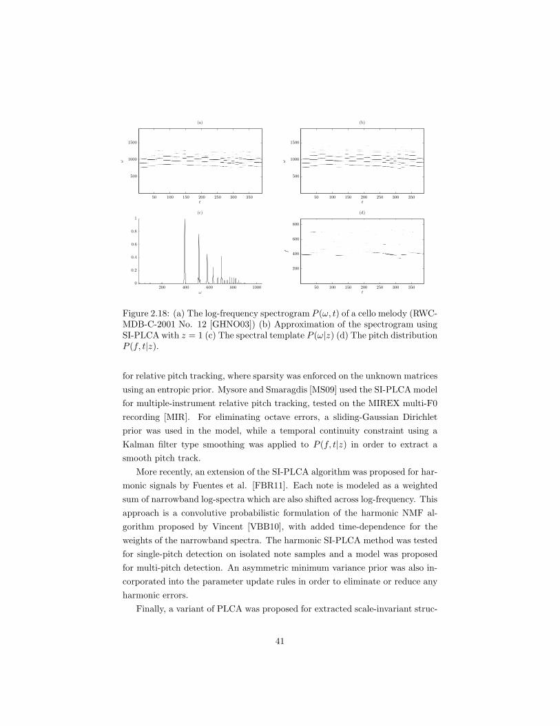
f
t
(d)
ω
(c)
ω
t
(b)ω
t
(a)
50 100 150 200 250 300 350200 400 600 800 1000
50 100 150 200 250 300 35050 100 150 200 250 300 350
200
400
600
800
0
0.2
0.4
0.6
0.8
1
500
1000
1500
500
1000
1500
Figure 2.18: (a) The log-frequency spectrogram P (ω, t) of a cello melody (RWC-MDB-C-2001 No. 12 [GHNO03]) (b) Approximation of the spectrogram usingSI-PLCA with z = 1 (c) The spectral template P (ω|z) (d) The pitch distributionP (f, t|z).
for relative pitch tracking, where sparsity was enforced on the unknown matrices
using an entropic prior. Mysore and Smaragdis [MS09] used the SI-PLCA model
for multiple-instrument relative pitch tracking, tested on the MIREX multi-F0
recording [MIR]. For eliminating octave errors, a sliding-Gaussian Dirichlet
prior was used in the model, while a temporal continuity constraint using a
Kalman filter type smoothing was applied to P (f, t|z) in order to extract a
smooth pitch track.
More recently, an extension of the SI-PLCA algorithm was proposed for har-
monic signals by Fuentes et al. [FBR11]. Each note is modeled as a weighted
sum of narrowband log-spectra which are also shifted across log-frequency. This
approach is a convolutive probabilistic formulation of the harmonic NMF al-
gorithm proposed by Vincent [VBB10], with added time-dependence for the
weights of the narrowband spectra. The harmonic SI-PLCA method was tested
for single-pitch detection on isolated note samples and a model was proposed
for multi-pitch detection. An asymmetric minimum variance prior was also in-
corporated into the parameter update rules in order to eliminate or reduce any
harmonic errors.
Finally, a variant of PLCA was proposed for extracted scale-invariant struc-
41

tures from linear frequency spectrograms in [HBD11b], which is equivalent to
extracting shift-invariant structures in log-frequency spectrograms. This scale-
invariant PLCA is useful for detecting frequency shifts when a linear frequency
representation such as the STFT is used. This can be useful for reconstructing
individual sources, which might not be possible when a log-frequency represen-
tation is utilised.
Non-negative Hidden Markov Model
NMF and PLCA are not able to handle non-stationarity in signals. Their convo-
lutive counterparts, NMD and SI-PLCA are able to extract 2-D structures from
a time-frequency representation, which could assist in detecting non-stationary
events. However, the dimensions of these 2-D structures are fixed, making the
models not suitable for music signal analysis, where notes do not have a fixed
duration. To that end, Mysore in [Mys10, MSR10] introduced temporal con-
straints into the PLCA model for music signal analysis and source separation.
This non-negative hidden Markov model (NHMM) expressed each component
using a set of spectral templates linked to a hidden state in an HMM. Thus,
temporal constraints can be introduced in the NMF framework for modeling
non-stationary events.
In the non-negative hidden Markov model, the input spectrogram Vω,t is
decomposed into a series of spectral templates per component and state, with
corresponding time-varying mixture weights for the components. The model in
terms of the observations is formulated as:
Pt(ωt|qt) =∑
zt
Pt(zt|qt)P (ωt|zt, qt) (2.21)
where P (ωt|zt, qt) denotes the spectral template for component z and state q,
and Pt(zt|qt) are the time-varying mixture weights. The use of subscript t in
Pt(·) means that there is a separate distribution for each time frame. The sub-
script t in random variables zt, ωt, qt refers to the value of the random variable
for the specific time frame. Pt(ωt|qt) is the time-varying observation probabil-
ity used in the HMM. Thus, the normalized spectrum of each time frame is
approximated by:
Pt(ω) =∑
qt
Pt(ωt|qt)Pt(qt) (2.22)
where Pt(qt) is the state activation, which can be computed using the HMM
42
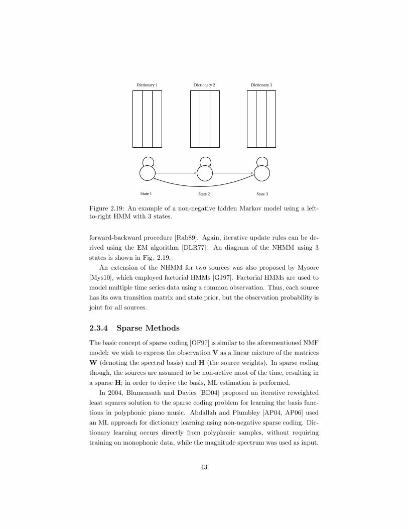
Dictionary 1 Dictionary 2 Dictionary 3
State 1 State 2 State 3
Figure 2.19: An example of a non-negative hidden Markov model using a left-to-right HMM with 3 states.
forward-backward procedure [Rab89]. Again, iterative update rules can be de-
rived using the EM algorithm [DLR77]. An diagram of the NHMM using 3
states is shown in Fig. 2.19.
An extension of the NHMM for two sources was also proposed by Mysore
[Mys10], which employed factorial HMMs [GJ97]. Factorial HMMs are used to
model multiple time series data using a common observation. Thus, each source
has its own transition matrix and state prior, but the observation probability is
joint for all sources.
2.3.4 Sparse Methods
The basic concept of sparse coding [OF97] is similar to the aforementioned NMF
model: we wish to express the observation V as a linear mixture of the matrices
W (denoting the spectral basis) and H (the source weights). In sparse coding
though, the sources are assumed to be non-active most of the time, resulting in
a sparse H; in order to derive the basis, ML estimation is performed.
In 2004, Blumensath and Davies [BD04] proposed an iterative reweighted
least squares solution to the sparse coding problem for learning the basis func-
tions in polyphonic piano music. Abdallah and Plumbley [AP04, AP06] used
an ML approach for dictionary learning using non-negative sparse coding. Dic-
tionary learning occurs directly from polyphonic samples, without requiring
training on monophonic data, while the magnitude spectrum was used as input.
43
Convolutive sparse coding for sound source separation was presented by
Virtanen in [Vir04], which is linked to non-negative matrix deconvolution pre-
sented in subsection 2.3.3. As in NMD, the resulting spectrum is considered to
be produced by a convolution of source basis spectrograms and onset vectors. In
addition, instead of a Euclidean distance-based cost function, a model fitting cri-
terion based on loudness perception is proposed. Shift-invariant sparse coding,
which is equivalent to convolutive sparse coding, was proposed in [MSH08] for
automatic transcription in multi-instrument mixtures. In that case, the model
extracts a spectral template per instrument source, which is shifted across log-
frequency, as in SI-PLCA.
Derrien et al. [Der06] proposed a method for the decomposition of music
spectrograms, based on the matching pursuit (MP) algorithm. A dictionary of
atoms in the log-frequency scale was used and comparisons were made with the
constant-Q spectrogram using a piano piece by Mozart.
Bertin et al. [BBR07] compared NMF with non-negative K-SVD, which is
a sparse coding-like algorithm for image coding. The l0 norm was used as a
sparsity measure, and the algorithms’ performance was found similar, although
NMF is preferred due to its lower computational cost (even though in NMF
sparsity is an uncontrolled side-effect).
Canadas-Quesada et al. [QCR+08] proposed a note detection approach based
on the harmonic matching pursuit (HMP) algorithm. The obtained atoms are
further processed using an algorithm based on the spectral smoothness princi-
ple. Also, Carabias-Orti et al. [OCQR10] proposed an unsupervised process for
learning spectral patterns of notes using the matching pursuit (MP) algorithm.
Spectral patterns are learned using additional constraints on harmonicity, enve-
lope smoothness, temporal continuity, and stability. The learned patterns are
used in a note-event detection system, where the harmonic atoms are clustered
according to the amplitude distribution of their spectral envelopes.
Sparse coding of Fourier coefficients was also used in [LYC11] for piano
transcription. The sparse representation is solved by l1 minimization, while a
postprocessing step for note tracking is applied using pitch-wise hidden Markov
models. This method was also publicly evaluated in [LYLC10] for the MIREX
piano note tracking task. The model can be formulated as:
ht = argmin ||ht||1, s.t. vt = Wht (2.23)
where vt is the input spectral vector at frame t, W is the dictionary matrix,
44
and ht is the activation of the dictionary atoms. || · ||1 refers to the l1 norm. A
method for automatic transcription using exemplar-based sparse representations
was also proposed by the same authors in [LYC12]. In this method, a piano
music segment is expressed as a linear combination of a small number of note
exemplars from a dictionary. The drawback of this method is that it requires
note samples from the same source as the recording (although it does not require
as many samples as the note range of the instrument).
In [OP11] a method for structure-aware dictionary learning is proposed and
applied to piano transcription, which takes into account harmonicity in mu-
sic spectra. Modifications on the NMF and K-SVD algorithms were made by
incorporating structure-awareness. More recently in [ONP12], structured spar-
sity (also called group sparsity) was applied to piano transcription. In group
sparsity, groups of atoms tend to be active at the same time.
Finally in [Sma11], the notion of exemplars was also utilised for polyphonic
pitch tracking. The method is formulated as a nearest subspace search problem.
The input time-frequency representation is a normalized magnitude spectro-
gram, which as in the PLCA case, can exploit the l2 norm for enforcing sparsity
on the atom activations. The problem requires the minimization of the following
cost function:
D[vt|W · ht]− ρ∑
i
h2i,t (2.24)
where W is the dictionary matrix, vt the spectrum of the input signal, ht is the
atom activation for the t-th frame, hi,t the activation value for the i-th atom, and
ρ is the sparsity parameter. In [Sma11], D[·] was set to be the Kullback-Leibler
divergence.
2.3.5 Machine Learning Methods
A limited number of methods in the literature use standard machine learning
techniques in order to estimate multiple F0s in frame-based systems. Chien
and Jeng in [CJ02] proposed a signal processing-based system which solved the
octave detection problem using a support vector machine (SVM) classifier. The
constant-Q transform was used as input and the features used to train the SVM
classifiers (one classifier for each pitch) were the partial amplitudes within a
short period of time following an onset.
Marolt in [Mar04] performed a comparison of neural networks for note recog-
nition, using as input features the output values of oscillator networks. A net-
45
work of adaptive oscillators was used for tracking the partials of each pitch. The
best performance was reported for the time-delay neural networks (TDNNs).
Pertusa and Inesta in [PI04, PI05] also used TDNNs for polyphonic music
transcription, where the input consisted of pre-processed STFT bins. Poliner
and Ellis [PE07a, PE07b] also used STFT bins for frame-level piano note clas-
sification using one-versus-all SVMs. In order to improve transcription per-
formance, the classification output of the SVMs was fed as input to a hidden
Markov model (HMM) for post-processing.
Giubin and Sheng [GS07a] proposed a transcription method which used a
backpropagation neural network for classification. The input features were de-
rived from an adaptive comb filter using an FFT as input. The system also
supported the detection of onsets, repeated notes, as well as note duration and
loudness estimation.
Zhou [Zho06] also used two-class SVMs for a comparative system for multiple-
F0 estimation, using as features spectral peak amplitudes extracted from the
RTFI representation. Gang et al. [GBHL09] employed a max-margin classifier
for polyphonic music transcription, where features derived from partial ampli-
tudes were used.
Costantini et al [CPT09] also employed SVMs for note classification and off-
set detection in piano recordings. The input time-frequency representation was
the constant-Q transform (CQT). The CQT bins were used as features for the
SVM classifier. It should be mentioned that this system performs classification
at the time instants of each note onset, estimated from an onset detector.
Ortiz et al. [OBBC10] proposed a lightweight pitch detector to be used in
embedded systems. A multilayer perceptron was used for classification, while
the Goertzel Algorithm was employed for computing the frequency components
of the signal on a log-frequency scale, which are used as features.
Nam et al. [NNLS11] employed deep belief networks for polyphonic piano
transcription. Training was made using spectrogram bins as features and using
both single notes and note combinations. For note tracking, the pitch-wise
HMMs from [PE07a] were used.
Finally, Bock and Schedl [BS12] used recurrent neural networks for poly-
phonic piano transcription. Features consist of the output of two semitone
filterbanks, one with short and one with a long window frame. A bidirectional
long short-term memory (BLSTM) neural network is used for note classification
and onset detection. In Fig. 2.20, the system diagram of the method proposed
by [BS12] can be seen.
46

Audio Notes
Spectrogram
46.4ms
Spectrogram
185.5ms
Semitone
Filterbank
Semitone
Filterbank
BLSTM
Network
Note Onset &
Pitch Detection
Figure 2.20: System diagram of the piano transcription method in [BS12].
2.3.6 Genetic Algorithm Methods
A radically different approach for automatic music transcription is the use of
genetic algorithms. Essentially, a transcription is estimated which is mutated
using a genetic algorithm until it matches some criterion. In the case of pro-
posed approaches for transcription using genetic algorithms, this criterion is
the similarity between the original signal and the synthesized signal from the
estimated transcription.
In [Fon08, FF09], a possible piano-roll transcription is estimated from frag-
ments defined by note onsets, is synthesized, and is compared with the original
spectrogram. The procedure is iterated by mutating the piano-roll, until conver-
gence is observed. In [Lu06], the same basic procedure is employed, although the
features used for synthesizing the transcription are pitch, timbre and dynamics.
Mutations employed by the proposed method in [Lu06] include a random note
change, a change in note duration, note split, note reclassification, and note
assimilation.
Finally, in [RFdVF08] a hybrid genetic algorithm based on gene fragment
competition was proposed for polyphonic music transcription. The proposed
method performs a quasi-global/quasi-local search by means of gene fragment
evaluation and selection using as feature the STFT peaks of the original signal.
A similar method was also publicly evaluated in the MIREX multiple-F0 and
note tracking task by the same authors in [RFF11], where the current fitness
function for the genetic algorithm is based on the log-spectral distance between
the spectra of the original and synthesized recordings.
2.4 Note Tracking
Typically automatic transcription algorithms compute a time-pitch representa-
tion such as a pitch activation matrix, which needs to be further processed in
order to detect note events (i.e. with note onsets and offsets). This procedure is
47
called note tracking or note smoothing. Most spectrogram factorization methods
estimate the binary piano-roll representation from the pitch activation matrix
using simple thresholding [GE11, Nie08, VBB08]. In [GE11] is is shown that
the proposed PLCA-based algorithm is fairly robust to the choice of threshold.
One simple and fast solution for note tracking is minimum duration pruning
[DCL10], which is applied after thresholding. Essentially, note events which
have a duration smaller than a predefined value are removed from the final
piano-roll. This method was also used in [BDS06], where more complex rules
for note tracking were used, such as in the case where a small gap exists between
two note events.
In [PE07a], a computationally inexpensive note tracking method was pro-
posed, in order to post-process the non-binary posteriogram of SVM classi-
fiers which were used for multi-pitch estimation. In this approach, pitch-wise
hidden Markov models were used, where each HMM has two states, denot-
ing note activity and inactivity. The HMM parameters (state transitions and
priors) were learned directly from a ground-truth training set, while the ob-
servation probability is given by the posteriogram output for a specific pitch.
The Viterbi algorithm [Rab89] is used for computing the optimal state se-
quence for each pitch, thus producing the final piano-roll. Given a pitch-
wise state sequence Q(p) = q(p)t , t = 1, . . . , T and a sequence of observations
O(p) = o(p)t , t = 1, . . . , T , the optimal state sequence is achieved by maximiz-
ing: ∏
t
P (o(p)t |q
(p)t )P (q
(p)t |q
(p)t−1) (2.25)
where p = 1, . . . ,P denotes pitch, P (q(p)t |q
(p)t−1) is the state transition matrix for
a given pitch, and P (o(p)t |q
(p)t ) is the pitch-wise observation probability. The
graphical structure of the pitch-wise HMM proposed in [PE07a] can be seen in
Fig. 2.21. An example of the note tracking procedure of [PE07a] can be seen in
Fig. 2.22, where the pitch activation output of an NMF-based algorithm with
β-divergence is used for HMM-based note tracking. This method has also been
employed for other transcription systems, e.g. [QRC+10], where P (o(p)t |q
(p)t )
was computed using the pitch salience as input to an exponential probability
density function (PDF). The note tracking method of [PE07a] was also used in
[LYLC10].
A more complex HMM architecture was proposed in [EBD08] for note track-
ing, where each HMM state corresponds to note combinations (more specifically,
48

q(p)1 q
(p)2 q
(p)3
o(p)1 o
(p)2 o
(p)3
...
Figure 2.21: Graphical structure of the pitch-wise HMM of [PE07a].
chords). As in [PE07a], note combination transitions and priors were learned
from MIDI data. However, it should be noted that the number of states is large:∑Ll=0
(Nc
L
), where L is the maximum polyphony level and Nc is the set of pitch
candidates.
Finally in [ROS09b], dynamic Bayesian networks (DBNs) were proposed for
note tracking using as input the pitch activation of an NMF-based multipitch
detection algorithm. The DBN has a note layer in the lowest level, followed by
a note combination layer. Model parameters were learned using MIDI files from
F. Chopin piano pieces.
2.5 Evaluation metrics
Evaluation of automatic transcription systems is typically done in two ways:
frame-based evaluation and note-based evaluation.
2.5.1 Frame-based Evaluation
Frame-based evaluations are made by comparing the transcribed output and
the ground-truth frame by frame typically using a 10 ms step, as in the MIREX
multiple-F0 estimation task [MIR]. A commonly employed metric is the overall
accuracy, defined by Dixon in [Dix00]:
Acc1 =
∑nNtp [n]∑
nNfp [n] +Nfn [n] +Ntp [n](2.26)
where Ntp [n] is the number of correctly detected pitches at frame n, Nfn [n]
denotes the number of false negatives, and Nfp [n] the number of false positives.
49

MID
Ipitch
time (10ms step)
(b)
MID
Ipitch
(a)
500 1000 1500 2000 2500 3000
500 1000 1500 2000 2500 3000
30
40
50
60
70
80
90
30
40
50
60
70
80
90
Figure 2.22: An example of the note tracking procedure of [PE07a].(a) The NMF-based pitch activation of the first 30 sec of ‘MAPS MUS-alb se2 ENSTDkCl’ from the MAPS database [EBD10]. (b) The output ofthe HMM-based note tracking step.
In the MIREX task, a variant of Acc1 is also used, called ‘Chroma Accuracy’
(Acc1c), where the reference ground-truth and transcribed output are warped
to one octave.
A second accuracy metric is also used for evaluation, proposed in [KNS07],
which also takes into account pitch substitutions:
Acc2 =
∑nNref [n]−Nfn [n]−Nfp [n] +Nsubs [n]∑
nNref [n](2.27)
where Nref [n] is the number of ground-truth pitches at frame n and Nsubs [n] is
the number of pitch substitutions, given by Nsubs [n] = min(Nfn [n], Nfp [n]).
The frame-wise precision, recall, and F-measure metrics are also used for
50
evaluating transcription systems, defined in [VBB10] as:
Pre =
∑nNtp [n]∑nNsys [n]
Rec =
∑nNtp [n]∑nNref [n]
F =2 · Rec · Pre
Rec + Pre(2.28)
where Nsys [n] is the number of detected pitches for the n-th frame.
From the aforementioned definitions, several error metrics have been defined
in [PE07a] that measure the substitution errors (Esubs), missed detection errors
(Efn), false alarm errors (Efp), and the total error (Etot ):
Esubs =
∑nmin(Nref [n], Nsys [n])−Ncorr [n]∑
nNref [n]
Efn =
∑nmax(0, Nref [n]−Nsys [n])∑
nNref [n]
Efp =
∑nmax(0, Nsys [n]−Nref [n])∑
nNref [n]
Etot = Esubs + Efn + Efp (2.29)
It should be noted that the aforementioned error metrics can exceed 100% if
the number of false alarms is very high [PE07a].
2.5.2 Note-based Evaluation
For note-based evaluation, the output of a transcription system is typically
in MIDI-like format, stating for each note event an onset, an offset, and the
respective pitch. In this case, the evaluation is more straightforward. There
are two ways of evaluating transcription algorithms using note-based metrics:
firstly, by only utilizing information from note onsets and secondly by using
information from onsets and offsets.
For onset-only evaluation, according to the MIREX [MIR] specifications, a
note event is assumed to be correct if its onset is within a ±50 ms range of a
ground-truth onset and its F0 is within ± a quarter tone (3%) of the ground-
truth pitch. For this case, metrics are defined in a similar way to (2.28), resulting
in the onset-only note-based precision, recall, and F-measure, denoted as Preon ,
Recon , and Fon , respectively.
For onset-offset evaluation, the same rules apply as in the onset-only evalua-
tion, plus the offset of each note needs to be within 20% of ground-truth note’s
duration around the ground-truth note’s offset value, or within 50 milliseconds
of the ground-truth notes offset, whichever is larger [BED09b]. Again, preci-
51

sion, recall, and F-measure metrics are defined in a similar way to (2.28), being
Preoff , Recoff , and Foff , respectively.
2.6 Public Evaluation
Public evaluations of various multiple-F0 estimation and note tracking ap-
proaches are carried out as part of the Music Information Retrieval Evaluation
eXchange (MIREX) framework [MIR]. Multiple-F0 estimation is evaluated in a
frame-based manner, while the note tracking task performs evaluation for note-
based events. For note tracking, two separate evaluations are made, one for
multiple-instrument transcription and one for piano-only transcription. Results
for the note tracking task are given using onset-only information, and using
both note onsets and offsets.
Currently, the dataset used for evaluation consists of 30 recordings of 30 sec
duration taken from a woodwind quintet recording of L. van Beethoven’s Vari-
ations for String Quartet, Op.18 No. 5 and synthesized pieces from the RWC
database [GHNO03]. The dataset also includes ten 30 sec recordings recorded
from a Disklavier piano [PE07a]. A 5-track woodwind recording is used as a de-
velopment dataset4, which was annotated by the author and Graham Grindlay.
An overview of the results for the MIREX multiple-F0 estimation and note
tracking tasks for 2007-2008 was made in [BED09b]. For these years, 16 algo-
rithms from 12 labs and 11 algorithms from 7 labs were tested, respectively. For
the multiple F0 estimation task, the best results were reported by the methods
proposed by Yeh [Yeh08], Pertusa and Inesta [PI08], Ryynanen and Klapuri
[RK05], and Zhou and Reiss [ZR08]. All of the aforementioned approaches em-
ploy signal processing techniques for multiple-F0 estimation without any learn-
ing procedures or statistical models (Ryynanen’s method employs HMMs in a
post-processing step). For the note tracking task, the best results were also
reported by the methods proposed by Yeh, Ryynanen and Klapuri, and Zhou
and Reiss, followed by the SVM-based approach by Poliner and Ellis [PE07a].
As far as runtimes were concerned, the most efficient algorithm was the one by
Zhou [ZR07], followed by the algorithm by Pertusa [PI08].
Best results for the multiple-F0 estimation task for years 2009-2011 are pre-
sented in Table 2.3. In 2009, the best results for the multiple-F0 estimation task
were also reported by Yeh [Yeh08], followed by the statistical modelling method
4http://www.music-ir.org/evaluation/MIREX/data/2007/multiF0/ (password required)
52
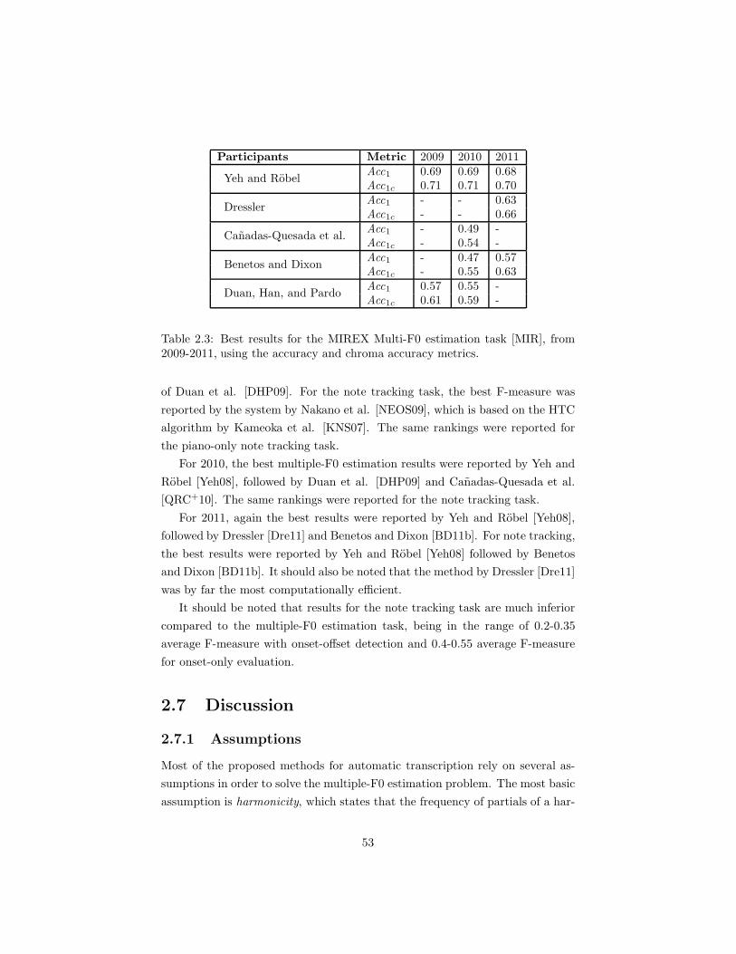
Participants Metric 2009 2010 2011
Yeh and RobelAcc1 0.69 0.69 0.68Acc1c 0.71 0.71 0.70
DresslerAcc1 - - 0.63Acc1c - - 0.66
Canadas-Quesada et al.Acc1 - 0.49 -Acc1c - 0.54 -
Benetos and DixonAcc1 - 0.47 0.57Acc1c - 0.55 0.63
Duan, Han, and PardoAcc1 0.57 0.55 -Acc1c 0.61 0.59 -
Table 2.3: Best results for the MIREX Multi-F0 estimation task [MIR], from2009-2011, using the accuracy and chroma accuracy metrics.
of Duan et al. [DHP09]. For the note tracking task, the best F-measure was
reported by the system by Nakano et al. [NEOS09], which is based on the HTC
algorithm by Kameoka et al. [KNS07]. The same rankings were reported for
the piano-only note tracking task.
For 2010, the best multiple-F0 estimation results were reported by Yeh and
Robel [Yeh08], followed by Duan et al. [DHP09] and Canadas-Quesada et al.
[QRC+10]. The same rankings were reported for the note tracking task.
For 2011, again the best results were reported by Yeh and Robel [Yeh08],
followed by Dressler [Dre11] and Benetos and Dixon [BD11b]. For note tracking,
the best results were reported by Yeh and Robel [Yeh08] followed by Benetos
and Dixon [BD11b]. It should also be noted that the method by Dressler [Dre11]
was by far the most computationally efficient.
It should be noted that results for the note tracking task are much inferior
compared to the multiple-F0 estimation task, being in the range of 0.2-0.35
average F-measure with onset-offset detection and 0.4-0.55 average F-measure
for onset-only evaluation.
2.7 Discussion
2.7.1 Assumptions
Most of the proposed methods for automatic transcription rely on several as-
sumptions in order to solve the multiple-F0 estimation problem. The most basic
assumption is harmonicity, which states that the frequency of partials of a har-
53

monic sequence are placed at integer multiples of the fundamental. In practice
though, in certain instruments (e.g. piano) partials are slightly shifted upwards
in frequency due to the inharmonicity phenomenon which needs to be taken
into account [Kla04a]. Inharmonicity occurs due to string stiffness, where all
partials of an inharmonic instrument have a frequency that is higher than their
expected harmonic value [BQGB04].
A commonly used model for automatic transcription which supports inhar-
monicity considers a pitch p of a musical instrument sound with fundamental
frequency fp,0 and inharmonicity coefficient bp. The partials for that sound are
located at frequencies:
fp,h = hfp,0
√1 + (h2 − 1)bp (2.30)
where h ≥ 1 is the partial index [KD06].
One of the most common assumptions used is spectral smoothness [BJ05,
Cau99, EBD10, Kla03, PI08, Yeh08], which assumes that the spectral envelope
of a pitched sound is smooth, although that assumption frequently does not
appear to be valid. An example of that case can be seen in Figure 2.23, where
the envelope of a trumpet sound forms a smooth contour, unlike the envelope
of a clarinet sound, where even partials have lower amplitude compared to the
odd ones.
Another assumption, which is implied for the spectral smoothness principle
and is employed in subspace-based additive models is power summation [dC06],
where it is assumed that the amplitude of two coinciding partials equals the
sum of their respective amplitudes. In fact though, considering two coincid-
ing partials with amplitudes a1 and a2, the resulting amplitude is given by
a = |a1 + a2ei∆φ|, where ∆φ is their phase difference [Kla01]. This assump-
tion can lead to estimation problems in the presence of harmonically-related
pitches (pitches whose fundamental frequencies are in a rational number rela-
tion), which are frequently found in Western music. Also, when used explicitly
in iterative approaches for multiple-F0 estimation (like [Kla03]), it can lead to
signal corruption. In practice, the resulting amplitude is often considered to
be the maximum of the two [dC06]. The power summation assumption is also
implied in all spectrogram factorization approaches for automatic transcription,
which use an additive model for representing a spectrum.
Other assumptions frequently encountered in multiple-F0 estimation systems
include a constant spectral template for all pitches, as in [SKT+08]. Spectro-
54

Magnitude(dB)
Frequency (Hz)
0 1000 2000 3000 4000 5000-100
-50
0
(a)
Magnitude(dB)
Frequency (Hz)
0 1000 2000 3000 4000 5000-100
-50
0
(b)
Figure 2.23: Trumpet (a) and clarinet (b) spectra of a C4 tone (261Hz). Over-tones occur in positions determined by integer multiples of the fundamentalfrequency. In the trumpet case, the partial envelope produces a smooth con-tour, which is not the case for the clarinet.
gram factorization-based approaches usually consider one spectral template per
pitch, which is however not sufficient for characterizing sounds produced by
different instrument types, or even sounds produced by the same instrument
at different conditions (instrument model, dynamics, articulation). These ap-
proaches also consider a similar decay model for all partials using a constant
spectral template, when in fact higher partials decay more rapidly compared
to lower partials. The problem of using a constant spectral template was ad-
dressed using non-negative matrix deconvolution [Sma04a, Sma04b] and convo-
lutive sparse coding [Vir04], but a different issue arises because these algorithms
use constant 2D templates with fixed note lengths, which is not the case in real-
world music where notes have arbitrary durations.
55
2.7.2 Design Considerations
An overview of the design considerations that go into the development of a
multiple-F0 estimation system will be given. The first decision to be made is
selecting the time-frequency representation that will be used for the subsequent
analysis. As shown in Section 2.3, most approaches use the short-time Fourier
transform, due to its strong theoretic background and computational efficiency.
There are however several drawbacks using the STFT, such as the constant
frequency resolution which can create problems in detecting lower pitches. Us-
ing a log-frequency representation like the wavelet transform or the constant-Q
representation of sounds has the advantage that the spacing between individ-
ual harmonics is the same for all pitches [Sma09], unlike the STFT. To that
end, filterbank methods have been employed in the literature, trying to use
an auditory front-end in an effort to produce improved estimation performance.
The unitary model proposed by Meddis in [MH92, MO97] performs a non-linear
transform into each filterbank input, which can assist pitch detection in the case
of suppressed fundamentals, but can also create false spectral peaks in chord
roots [TK00] due to the half-wave rectification, making the model useful for
the monophonic case but problematic in the case of polyphonic western music,
where harmonic relations are quite common. Another approach for comput-
ing a T/F representation for transcription is to increase the FFT resolution,
using quadratic interpolation, parametric methods, or using non-stationary si-
nusoidal modelling techniques, such as the reassignment spectrum [Hai03], with
the drawback of increased computational cost.
Another choice concerns the algorithm for multiple-F0 estimation. Signal
processing methods for transcription (e.g. [Kla03, PI08, YRR10]) have proved
to be quite robust and computationally inexpensive. However, they are diffi-
cult to generalize and to control, since their performance is mostly based on a
combination of audio features and ad-hoc models. Spectrogram factorization
models and sparse decomposition approaches ([VBB08, GE11, LYC12]) seem
more appropriate for multi-pitch estimation, since they are based on a sim-
ple and transparent model which is easy to control and generalize. However,
most spectrogram factorization-based approaches are computationally expen-
sive and the results are sometimes not as high compared to signal processing-
based approaches. Furthermore, spectrogram factorization-based approaches
for multi-pitch detection are mostly based on the magnitude of the frequency or
log-frequency bins of a spectrogram, thus ignoring any additional features from
56

audio processing which might improve transcription performance. Although
machine learning methods have been shown to be appropriate for classification
problems, problems have been reported regarding their generalization perfor-
mance for the automatic transcription task (e.g. [PE07a]).
A third choice would be whether to perform multiple-F0 estimation on a
frame-by-frame basis and afterwards form the notes using the frame-based pitch
estimates or to jointly perform multipitch tracking. Only a few methods in the
literature perform multiple-F0 estimation and note tracking in a joint fashion,
due to the complexity of the problem. Such methods include the HTC algo-
rithm by Kameoka [KNS07], the HMM-based model by Chang [CSY+08], the
constrained clustering model proposed by Duan [DHP09], and the Poisson point
process model for multi-pitch detection combined with a dynamical model for
note transitions proposed by Bunch and Godsill [BG11]. Finally, another de-
sign consideration is whether the developed system is able to perform instrument
identification along with multi-pitch detection (e.g. [GE11]).
2.7.3 Towards a Complete Transcription
Most of the aforementioned transcription approaches tackle the problems of
multiple-F0 estimation and note onset and offset detection. However, in order
to fully solve the AMT problem and have a system that provides an output
that is equivalent to sheet music, additional issues need to be addressed, such as
metre induction, rhythm parsing, key finding, note spelling, dynamics, fingering,
expression, articulation and typesetting. Although there are approaches that
address many of these individual problems, there exists no ‘complete’ AMT
system to date.
Regarding typesetting, current tools produce readable scores from MIDI
data only (e.g. Lilypond5), ignoring cues from the music signal which could also
assist in incorporating additional information into the final score (e.g. expres-
sive features for note phrasing). As far as dynamics are concerned, in [EM11]
a method was proposed for estimating note intensities in a score-informed sce-
nario. However, estimating note dynamics in an unsupervised way has not been
tackled. Another issue would be the fact that most existing ground-truth does
not include note intensities, which is difficult to annotate manually, except for
datasets created using reproducing pianos (e.g. [PE07a]), which automatically
contain intensity information such as MIDI note velocities.
5http://lilypond.org/
57
Recent work [BKTB12] addresses the problem of automatically extract-
ing the fingering configurations for guitar recordings in an AMT framework.
For computing fingering, information from the transcribed signal as well as
instrument-specific knowledge is needed. Thus, a robust instrument identifica-
tion system would need to be incorporated for computing fingerings in multi-
instrument recordings.
For extracting expressive features, some work has been done in the past,
mostly in the score-informed case. In [GBL+11] a framework for extracting
expressive features both from a score-informed and an uninformed perspective
is proposed. In the latter case, an AMT system is used prior to the extraction of
expressive features. It should be mentioned though that the extracted features
(e.g. auditory loudness, attack, pitch deviation) do not necessarily correspond to
expressive notation. Thus, additional work needs to be done in order to provide
a mapping between mid-level expressive features and the expressive markings
in a final transcribed music score.
58

Chapter 3
Audio Feature-based
Automatic Music
Transcription
3.1 Introduction
This chapter presents proposed methods for multiple-F0 estimation of isolated
sounds as well as for complete recordings using techniques from signal processing
theory. Audio features are proposed which exploit the spectral structure and
temporal evolution of notes. Firstly, an iterative multiple-F0 estimation method
for isolated piano sounds is presented, which was published in [BD10a]. This
method is also converted into a system for automatic music transcription, which
was publicly evaluated in [BD10b].
Afterwards, a method for joint multiple-F0 estimation is proposed, which is
based on a novel algorithm for spectral envelope estimation in the log-frequency
domain. This method was published in [BD11a]. For this method, a novel
note tracking procedure was also utilized using conditional random fields. An
extension of the aforementioned system is also presented, which applies late
fusion-based onset detection and hidden Markov model-based offset detection,
which was published in [BD11d]. Finally, evaluation results are presented in
this chapter for all proposed methods.
59

AUDIO LOUDNESS
NORMALIZATION
RTFI
EXTRACTION
SPECTRAL
WHITENING
NOISE
SUPPRESSION
ONSET
DETECTION
PREPROCESSING
SALIENCE
FUNCTION
SPECTRAL STRUCTURE
RULES
TUNING & INHARMONICITY
ESTIMATION
TEMPORAL EVOLUTION
RULES
ESTIMATED PITCHES
MULTIPLE-F0 ESTIMATION
Figure 3.1: Diagram for the proposed multiple-F0 estimation system for isolatedpiano sounds.
3.2 Multiple-F0 Estimation of Piano Sounds
Initial research consists of a system for multiple-F0 estimation of isolated piano
sounds which uses candidate selection and several rule-based refinement steps.
The resonator time-frequency image (RTFI) is used as a data representation
[ZRMZ09], and preprocessing steps for noise suppression, spectral whitening,
and onset detection are utilized in order to make the estimation system robust
to noise and recording conditions. A pitch salience function that is able to
function in the log-frequency domain and utilizes tuning and inharmonicity
estimation procedures is proposed and pitch candidates are selected according
to their salience value. The set of candidates is refined using rules regarding the
harmonic partial sequence of the selected pitches and the temporal evolution of
the partials, in order to minimize errors occurring at multiples and sub-multiples
of the actual F0s. For the spectral structure rules, a more robust formulation
of the spectral irregularity measure [ZRMZ09] is proposed, taking into account
overlapping partials. For the temporal evolution rules, a novel feature based on
the common amplitude modulation (CAM) assumption [LWW09] is proposed
in order to suppress estimation errors in harmonically-related F0 candidates. A
diagram showing the stages of the proposed system is displayed in Figure 3.1.
60

3.2.1 Preprocessing
Resonator Time-Frequency Image
As a time-frequency representation, the resonator time-frequency image (RTFI)
is used [ZRMZ09]. The RTFI selects a first-order complex resonator filter
bank to implement a frequency-dependent time-frequency analysis. For the
specific experiments, a RTFI with constant-Q resolution is selected for the time-
frequency analysis, due to its suitability for music signal processing techniques,
because the inter-harmonic spacing is the same for all pitches. The time interval
between two successive frames is set to 40ms, which is typical for multiple-F0
estimation approaches [KD06]. The centre frequency difference between two
neighbouring filters is set to 10 cents (the number of bins per octave is set to
120). The frequency range is set from 27.5Hz (A0) to 12.5kHz (which reaches
up to the 3rd harmonic of C8). The employed absolute value of the RTFI will
be denoted as X [ω, t], where t is the time frame and ω the log-frequency bin.
Spectral Whitening and Noise Suppression
Spectral whitening (or flattening) is a key preprocessing step applied in multiple-
F0 estimation systems, in order to suppress timbral information and make the
following analysis more robust to different sound sources. When viewed from
an auditory perspective, it can be interpreted as the normalization of the hair
cell activity level [TK00].
Here, a modified version of the real-time adaptive whitening method pro-
posed in [SP07] is applied. Each band is scaled, taking into account the tem-
poral evolution of the signal, while the scaling factor is dependent only on past
frame values and the peak scaling value is exponentially decaying. The following
iterative algorithm is applied:
Y [ω, t] =
max(X [ω, t], θ, Y [ω, t− 1]), t > 0
max(X [ω, t], θ), t = 0
X [ω, t] ←X [ω, t]
Y [ω, t](3.1)
where < 1 is the peak scaling value and θ is a floor parameter.
In addition, a noise suppression approach similar to the one in [Kla09b] is em-
ployed, due to its computational efficiency. A half-octave span (60 bin) moving
median filter is computed for Y [ω, t], resulting in noise estimate N [ω, t]. After-
61

wards, an additional moving median filter N ′[ω, t] of the same span is applied,
but only including the RTFI bins whose amplitude is less than the respective
amplitude of N [ω, t]. This results in making the noise estimate N ′[ω, t] robust
in the presence of spectral peaks that could affect the noise estimate N [ω, t].
Onset Detection
In order to select the steady-state area of the piano tone (or tones), a spectral
flux-based onset detection procedure is applied. The spectral flux measures the
positive magnitude changes in each frequency bin, which indicate the attack
parts of new notes [BDA+05]. It can be used effectively for onset detection of
notes produced by percussive instruments such as the piano, but its performance
decreases for the detection of soft onsets [Bel03]. For the RTFI, the spectral
flux using the ℓ1 norm can be defined as:
SF [t] =∑
ω
HW (|Y [ω, t]| − |Y [ω, t− 1]|) (3.2)
where HW (·) = ·+|·|2 is a half-wave rectifier. The resulting onset strength signal
is smoothed using a median filter with a 3 sample span (120ms length), in
order to remove spurious peaks. Onsets are subsequently selected from SF [t]
by a selection of local maxima, with a minimum inter-peak distance of 120 ms.
Afterwards, the frames located between 100-300 ms after the onset are selected
as the steady-state region of the signal and are averaged over time, in order to
produce a robust spectral representation of the tones.
3.2.2 Multiple-F0 Estimation
Salience Function
In the linear frequency domain, considering a pitch p of a piano sound with
fundamental frequency fp,0 and inharmonicity coefficient bp, partials are located
at frequencies:
fp,h = hfp,0
√1 + (h2 − 1)bp (3.3)
where h ≥ 1 is the partial index [KD06, BQGB04]. Consequently in the log-
frequency domain, considering a pitch p at bin ωp,0, overtones are located at
bins:
ωp,h = ωp,0 +
⌈u · log2(h) +
u
2log2
(1 + (h2 − 1)bp
)⌋(3.4)
62

where u = 120 refers to the number of bins per octave and ⌈·⌋ to the rounding
operator.
A pitch salience function S[p, δp, bp] operating in the log-frequency domain
is proposed, which indicates the strength of pitch candidates:
S[p, δp, bp] =
H∑
h=1
maxmh
√Y
[ωp,h + δp +
⌈umh +
u
2log2(1 + (h2 − 1)bp)
⌋]
(3.5)
where Y [ω] is the log-frequency spectrum for a specific time frame, δp ∈ [−4, . . . , 4]
is the tuning deviation for each pitch, and mh specifies a search range around
overtone positions, belonging to the interval (mlh,m
uh), where:
mlh =
⌈log2(h− 1) + (M − 1) log2(h)
M
⌋
muh =
⌈(M − 1) log2(h) + log2(h+ 1)
M
⌋(3.6)
M is a factor controlling the width of the interval, which after experimentation
was set to 60.
While the employed salience functions in the linear frequency domain (e.g.
[Kla09b]) used a constant search space for each overtone, the proposed log-
frequency salience function sets the search range around each partial to be
inversely proportional to the partial index. The number of considered overtones
H is set to 11 at maximum. A tuning search space of 50 cents is set around
the ideal tuning frequency. The range of the inharmonicity coefficient bp is set
between 0 and 5 · 10−4, which is typical for piano notes [BQGB04].
In order to accurately estimate the tuning factor and the inharmonicity
coefficient for each pitch, a two-dimensional maximization procedure using ex-
haustive search is applied to S[p, δp, bp] for each pitch p ∈ [21, . . . , 108] in the
MIDI scale (corresponding to a note range of A0-C8). This results in a pitch
salience function estimate S ′[p], a tuning deviation vector and an inharmonicity
coefficient vector. Using the information extracted from the tuning and inhar-
monicity estimation, a harmonic partial sequence HPS [p, h] for each candidate
pitch and its harmonics (which contains the RTFI values at certain bin) is also
stored for further processing.
An example of the salience function generation is given in Fig. 3.2, where
the RTFI spectrum of an isolated F♯3 note played by a piano is seen, along
with its corresponding salience S ′[p]. The highest peak in S ′[p] corresponds to
63

ω
(a)
p
(b)
20 30 40 50 60 70 80 90 100 110
0 200 400 600 800 1000 1200
0
2
4
6
0
1
2
3
Figure 3.2: (a) The RTFI slice Y [ω] of an F♯3 piano sound. (b) The correspond-ing pitch salience function S ′[p].
p = 54, thus F♯3.
Spectral Structure Rules
A set of rules examining the harmonic partial sequence structure of each pitch
candidate is applied, which is inspired by work from [Bel03, Zho06]. These rules
aim to suppress peaks in the salience function that occur at multiples and sub-
multiples of the actual fundamental frequencies. In the semitone space, these
peaks occur at ±12, 19, 24, 28, . . . semitones from the actual pitch. The set-
tings for the rules were made using a development set from the MAPS database
[EBD10], as described in subsection 3.5.1.
A first rule for suppressing salience function peaks is setting a minimum
number for partial detection in HPS [p, h], similar to [Bel03, Zho06]. If p < 47,
at least three partials out of the first six need to be present in the harmonic
partial sequence (allowing for cases such as a missing fundamental). If p ≥ 47,
at least four partials out of the first six should be detected. A second rule
concerns the salience value, which expresses the sum of the square root of the
partial sequence amplitudes. If the salience value is below a minimum threshold
(set to 0.2 using the development set explained in Section 3.5), this peak is
suppressed. Another processing step in order to reduce processing time is the
64
reduction of the number of pitch candidates [EBD10], by selecting only the
pitches with the greater salience values. In the current experiments, up to 10
candidate pitches are selected from S ′[p].
Spectral flatness is another descriptor that can be used for the elimination
of errors occurring in subharmonic positions [EBD10]. In the proposed system,
the flatness of the first 6 partials of a harmonic sequence is used:
Fl [p] =
6
√∏6h=1 HPS [p, h]
∑6h=1 HPS [p,h]
6
(3.7)
The ratio of the geometric mean of HPS [p] to its arithmetic mean gives a mea-
sure of smoothness; a high value of Fl [p] indicates a partial sequence with a
smooth envelope, while a lower value indicates fluctuations in the partial val-
ues, which could indicate the presence of a falsely detected pitch occurring in a
sub-harmonic position. For the current experiments, the lower Fl [p] threshold
for suppressing pitch candidates was set to 0.1 after experimentation using the
development set (described in Section 3.5).
In order to suppress candidate pitches occurring at multiples of the true
fundamental frequency, a modified version of the spectral irregularity measure
formulated in [ZRMZ09] is proposed. Considering a pitch candidate with fun-
damental frequency f0 and another candidate with fundamental frequency lf0,
l > 1, spectral irregularity is defined as:
SI [p, l] =
3∑
h=1
HPS [p, hl]−HPS [p, hl− 1] +HPS [p, hl+ 1]
2(3.8)
The spectral irregularity is tested on pairs of harmonically-related candidate
F0s. A high value of SI [p, l] indicates the presence of the higher pitch with
fundamental frequency lf0, which is attributed to the higher energy of the shared
partials between the two pitches compared to the energy of the neighbouring
partials of f0.
In this work, the SI is modified in order to make it more robust against
overlapping partials that are caused by non-harmonically related F0s. Given
the current set of candidate pitches from S ′[p], the overlapping partials from
non-harmonically related F0s are detected as in [Yeh08] and smoothed according
to the spectral smoothness assumption, which states that the spectral envelope
of harmonic sounds should form a smooth contour [Kla03]. For each overlap-
65

ping partial HPS [p, h], an interpolated value HPS interp[p, h] is estimated by
performing linear interpolation using its neighbouring partials. Afterwards, the
smoothed partial amplitude HPS ′[p, h] is given by min(HPS [p, h],HPS interp[p, h]),
as in [Kla03]. The proposed spectral irregularity measure, which now takes the
form of a ratio in order to take into account the decreasing amplitude of higher
partials, is thus formed as:
SI ′[p, l] =3∑
h=1
2 ·HPS ′[p, hl]
HPS ′[p, hl − 1] +HPS ′[p, hl+ 1](3.9)
For each pair of harmonically-related F0s (candidate pitches that have a pitch
distance of ±12, 19, 24, 28, . . .) that are present in S ′[p] , the existence of the
higher pitch is determined by the value of SI ′ (for the current experiments, a
threshold of 1.2 was set using the development set).
Temporal Evolution Rules
Although the SI and the spectral smoothness assumption are able to suppress
some harmonic errors, additional information needs to be exploited in order to
produce more accurate estimates in the case of harmonically-related F0s. In
[Yeh08], temporal information was employed for multiple-F0 estimation using
the synchronicity criterion as a part of the F0 hypothesis score function. There,
it is stated that the temporal centroid for a harmonic partial sequence should
be the same for all partials. Thus, partials deviating from their global temporal
centroid indicates an invalid F0 hypothesis. Here, we use the common amplitude
modulation (CAM) assumption [GS07b, LWW09] in order to test the presence
of a higher pitch in the case of harmonically-related F0s. CAM assumes that
the partial amplitudes of a harmonic source are correlated over time and has
been used in the past for note separation given a ground truth of F0 estimates
[LWW09]. Thus, the presence of an additional source that overlaps certain
partials (e.g. in the case of an octave where even partials are overlapped) causes
the correlation between non-overlapped partials and the overlapped partials to
decrease.
To that end, tests are performed for each harmonically-related F0 pair that
is still present in S ′[p], comparing partials that are not overlapped by any non-
harmonically related F0 candidate with the partial of the fundamental. The
66
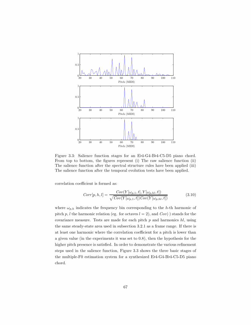
Pitch (MIDI)
Pitch (MIDI)
Pitch (MIDI)
20 30 40 50 60 70 80 90 100 110
20 30 40 50 60 70 80 90 100 110
20 30 40 50 60 70 80 90 100 110
0
0.5
1
0
0.5
1
0
0.5
1
Figure 3.3: Salience function stages for an E4-G4-B4-C5-D5 piano chord.From top to bottom, the figures represent (i) The raw salience function (ii)The salience function after the spectral structure rules have been applied (iii)The salience function after the temporal evolution tests have been applied.
correlation coefficient is formed as:
Corr [p, h, l] =Cov (Y [ωp,1, t], Y [ωp,hl, t])√
Cov (Y [ωp,1, t])Cov (Y [ωp,hl, t])(3.10)
where ωp,h indicates the frequency bin corresponding to the h-th harmonic of
pitch p, l the harmonic relation (eg. for octaves l = 2), and Cov (·) stands for the
covariance measure. Tests are made for each pitch p and harmonics hl, using
the same steady-state area used in subsection 3.2.1 as a frame range. If there is
at least one harmonic where the correlation coefficient for a pitch is lower than
a given value (in the experiments it was set to 0.8), then the hypothesis for the
higher pitch presence is satisfied. In order to demonstrate the various refinement
steps used in the salience function, Figure 3.3 shows the three basic stages of
the multiple-F0 estimation system for a synthesized E4-G4-B4-C5-D5 piano
chord.
67
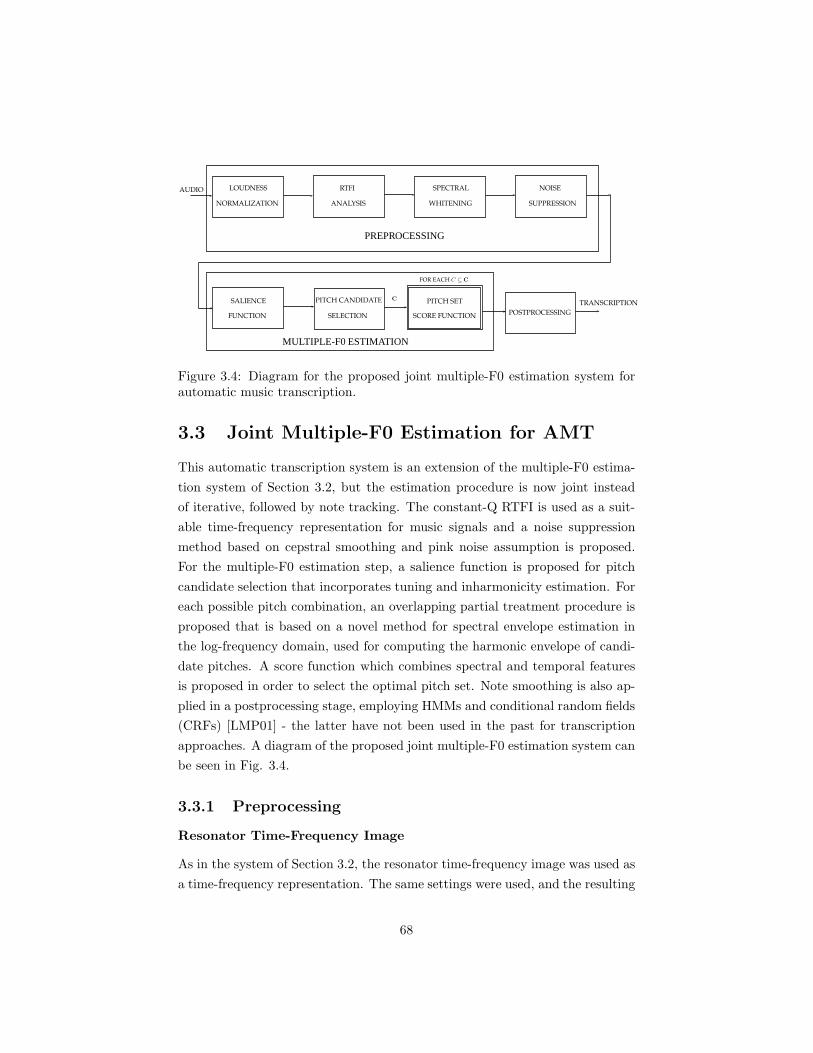
AUDIO LOUDNESS
NORMALIZATION
RTFI
ANALYSIS
SPECTRAL
WHITENING
NOISE
SUPPRESSION
PREPROCESSING
SALIENCE
FUNCTION
PITCH CANDIDATE
SELECTION
MULTIPLE-F0 ESTIMATION
PITCH SET
SCORE FUNCTION
FOR EACH C ⊆ C
POSTPROCESSING
TRANSCRIPTIONC
Figure 3.4: Diagram for the proposed joint multiple-F0 estimation system forautomatic music transcription.
3.3 Joint Multiple-F0 Estimation for AMT
This automatic transcription system is an extension of the multiple-F0 estima-
tion system of Section 3.2, but the estimation procedure is now joint instead
of iterative, followed by note tracking. The constant-Q RTFI is used as a suit-
able time-frequency representation for music signals and a noise suppression
method based on cepstral smoothing and pink noise assumption is proposed.
For the multiple-F0 estimation step, a salience function is proposed for pitch
candidate selection that incorporates tuning and inharmonicity estimation. For
each possible pitch combination, an overlapping partial treatment procedure is
proposed that is based on a novel method for spectral envelope estimation in
the log-frequency domain, used for computing the harmonic envelope of candi-
date pitches. A score function which combines spectral and temporal features
is proposed in order to select the optimal pitch set. Note smoothing is also ap-
plied in a postprocessing stage, employing HMMs and conditional random fields
(CRFs) [LMP01] - the latter have not been used in the past for transcription
approaches. A diagram of the proposed joint multiple-F0 estimation system can
be seen in Fig. 3.4.
3.3.1 Preprocessing
Resonator Time-Frequency Image
As in the system of Section 3.2, the resonator time-frequency image was used as
a time-frequency representation. The same settings were used, and the resulting
68

absolute value of the RTFI is denoted as X [ω, t].
Spectral Whitening
In this system, we employ a spectral whitening method similar to the one in
[KD06], but modified for log-frequency spectra instead of linear frequency ones.
For each frequency bin, the power within a subband of 13 octave span multiplied
by a Hann-window Whann[ω] is computed. The square root of the power within
each subband is:
σ[ω] =
(1
Ω
ω+Ω/2∑
l=ω−Ω/2
Whann[l]|X [l]|2)1/2
(3.11)
where Ω = u/3 = 40 bins and X [ω] is an RTFI spectrum. Afterwards, each bin
is scaled according to:
Y [ω] = (σ[ω])j−1X [ω] (3.12)
where j is a parameter which determines the amount of spectral whitening
applied and X [ω] is the absolute value of the RTFI for a single time frame, and
Y [ω] is the final whitened RTFI slice. As in [KD06], j was set to 0.33.
Noise Suppression
In [Yeh08], an algorithm for noise level estimation was proposed, based on the as-
sumption that noise peaks are generated from a white Gaussian process, and the
resulting spectral amplitudes obey a Rayleigh distribution. Here, an approach
based on a pink noise assumption (elsewhere called 1/f noise or equal-loudness
noise) is proposed. In pink noise, each octave carries an equal amount of energy,
which corresponds well to the approximately logarithmic frequency scale of hu-
man auditory perception. Additionally, it occurs widely in nature, contrary to
white noise and is also suitable for the employed time-frequency representation
used in this work.
The proposed signal-dependent noise estimation algorithm is as follows:
1. Perform a two-stage median filtering procedure on Y [ω], in a similar way to
[Kla09b], where a moving median average is calculated using the whitened
spectrum. A second moving median average is calculated, including only
the spectral bins that fall below the magnitude of the first moving average.
The span of the filter is set to 13 octave. The resulting noise representation
N [ω] gives a rough estimate of the noise level.
69

2. Using the noise estimate, a transformation from the log-frequency spectral
coefficients to cepstral coefficients is performed [Bro99]:
cξ =
Ω′∑
ω=1
log(N [ω]) cos
(ξ
(ω −
1
2
)π
Ω′
)(3.13)
where Ω′ = 1043 is the total number of log-frequency bins in the RTFI
and Ξ is the number of cepstral coefficients employed, ξ = 0, . . . ,Ξ− 1.
3. A smooth curve in the log-magnitude, log-frequency domain is recon-
structed from the first D cepstral coefficients:
log |Nc(ω)| ≈ exp
(c0 + 2
D−1∑
ξ=1
cξ · cos(ξω)
)(3.14)
4. The resulting smooth curve is mapped from ω into ω. Assuming that the
noise amplitude follows an exponential distribution, the expected value of
the noise log amplitudes Elog(|Nc(ω)|) is equal to log(λ−1)− γ, where
γ is the Euler constant (≈ 0.5772). Since the mean of an exponential
distribution is equal to 1λ , the noise level in the linear amplitude scale can
be described as:
LN (ω) = Nc(ω) · eγ (3.15)
The analytic derivation of Elog(|Nc(ω)|) can be found in Appendix A.
In this work, the number of cepstral coefficients used was set to D = 50. Let
Z[ω] stand for the whitened and noise-suppressed RTFI representation.
3.3.2 Multiple-F0 Estimation
In this subsection, multiple-F0 estimation, being the core of the proposed tran-
scription system, is described. Performed on a frame-by-frame basis, a pitch
salience function is generated, tuning and inharmonicity parameters are ex-
tracted, candidate pitches are selected, and for each possible pitch combination
an overlapping partial treatment is performed and a score function is computed.
Salience Function
The same salience function that is proposed in the multiple-F0 estimation sys-
tem of Section 3.2 is employed in this system. The final result of the salience
70
function computation stage is the pitch salience function estimate S ′[p], a tuning
deviation vector and an inharmonicity coefficient vector. Also, using the infor-
mation extracted from the tuning and inharmonicity estimation, a harmonic
partial sequence (HPS) HPS [p, h], which contains magnitude information from
Y [ω] for each harmonic of each candidate pitch, is also stored for further pro-
cessing.
Pitch Candidate Selection
As in the multiple-F0 estimation system of Section 3.2, a set of conservative
rules examining the harmonic partial sequence structure of each pitch candi-
date is applied, which is inspired by work from [Bel03, PI08]. For the present
system, these rules aim to reduce the pitch candidate set for computational
speed purposes.
A first rule for suppressing salience function peaks is setting a minimum num-
ber for partial detection in HPS [p, h], similar to [Bel03]. At least three partials
out of the first six need to be present in the harmonic partial sequence. A second
rule discards pitch candidates with a salience value less than 0.1max(S ′[p]), as
in [PI08].
Finally, after spurious peaks in S ′[p] have been eliminated, CN = 10 candi-
date pitches are selected from the highest amplitudes of S ′[p] [EBD10]. The set
of selected pitch candidates will be denoted as C. Thus, the maximum number of
possible pitch candidate combinations that will be considered is 210, compared
to 288 if the aforementioned procedures were not employed.
Overlapping Partial Treatment
Current approaches in the literature rely on certain assumptions in order to re-
cover the amplitude of overlapped harmonics. In [Kla03], it is assumed that har-
monic amplitudes decay smoothly over frequency (spectral smoothness). Thus,
the amplitude of an overlapped harmonic can be estimated from the ampli-
tudes of neighboring non-overlapped harmonics. In [VK02], the amplitude of
the overlapped harmonic is estimated through non-linear interpolation on the
neighboring harmonics. In [ES06], each set of harmonics is filtered from the
spectrum and in the case of overlapping harmonics, linear interpolation is em-
ployed.
In this system, an overlapping partial treatment procedure based on spec-
tral envelope estimation of candidate pitches is proposed. The proposed spec-
71
tral envelope estimation algorithm for the log-frequency domain is presented in
Appendix B. For each possible pitch combination C ⊆ C, overlapping partial
treatment is performed, in order to accurately estimate the partial amplitudes.
The proposed overlapping partial treatment procedure is as follows:
1. Given a set C of pitch candidates, estimate a partial collision list.
2. For a given harmonic partial sequence, if the number of overlapped partials
is less than Nover, then estimate the harmonic envelope SEp[ω] of the
candidate pitch using only amplitude information from non-overlapped
partials.
3. For a given harmonic partial sequence, if the number of overlapped partials
is equal to or greater than Nover, estimate the harmonic envelope using
information from the complete harmonic partial sequence.
4. For each overlapped partial, estimate its amplitude using the harmonic
envelope parameters of the corresponding pitch candidate (see Appendix
B).
The output of the overlapping partial treatment procedure is the updated
harmonic partial sequence HPS [p, h] for each pitch set combination.
Pitch set score function
Having selected a set of possible pitch candidates and performed overlapping
partial treatment on each possible combination, the goal is to select the optimal
pitch combination for a specific time frame. In [Yeh08], Yeh proposed a score
function which combined four criteria for each pitch: harmonicity, bandwidth,
spectral centroid, and synchronicity. Also, in [PI08], a simple score function
was proposed for pitch set selection, based on the smoothness of the pitch set.
Finally, in [EBD10] a multipitch detection function was proposed, which em-
ployed the spectral flatness of pitch candidates along with the spectral flatness
of the noise residual.
Here, a weighted pitch set score function is proposed, which combines spec-
tral and temporal characteristics of the candidate F0s, and also attempts to
minimize the noise residual to avoid any missed detections. Also, features which
concern harmonically-related F0s are included in the score function, in order to
suppress any harmonic errors. Given a candidate pitch set C ⊆ C with size |C|,
72

the proposed pitch set score function is:
L(C) =
|C|∑
i=1
(Lp(i)) + Lres (3.16)
where Lp(i) is the score function for each candidate pitch p(i) ∈ C, and Lres is
the score for the residual spectrum. Lp and Lres are defined as:
Lp = w1Fl [p] + w2Sm[p]− w3SC [p] + w4PR[p]− w5AM [p]
Lres = w6Fl [Res] (3.17)
Features Fl , Sr , SC ,PR,AM have been weighted by the salience function
of the candidate pitch and divided by the sum of the salience function of the
candidate pitch set, for normalization purposes. In order to train the weight
parameters wi, i = 1, . . . , 6 of the features in (3.17), we used the Nelder-Mead
search algorithm for parameter estimation [NM65]. The training set employed
for experiments is described in Section 3.5. The pitch candidate set that maxi-
mizes the score function:
C = argmaxC⊆C
L(C) (3.18)
is selected as the pitch estimate for the current frame.
Fl [p] denotes the spectral flatness of the harmonic partial sequence:
Fl [p] =e[∑
Hh=1 log(HPS [p,h])]/H
1H
∑Hh=1 HPS [p, h]
(3.19)
The spectral flatness is a measure of the ‘whiteness’ of the spectrum. Its values
lie between 0 and 1 and it is maximized when the input sequence is smooth,
which is the ideal case for an HPS. It has been used previously for multiple-F0
estimation in [PI08, EBD10]. Compared with (3.7), in (3.19) the definition is
the one adapted by the MPEG-7 framework, which can be seen in [Uhl10].
Sm[p] is the smoothness measure of a harmonic partial sequence, which
was proposed in [PI08]. The definition of smoothness stems from the spectral
smoothness principle and its definition stems from the definition of sharpness :
Sr [p] =
H∑
h=1
(SEp[ωp,h]−HPS [p, h]) (3.20)
73
Here, instead of a low-pass filtered HPS using a Gaussian window as in [PI08],
the estimated harmonic envelope SEp of each candidate pitch is employed for
the smoothness computation. Sr [p] is normalized into Sr [p] and the smoothness
measure Sm[p] is defined as: Sm[p] = 1− Sr [p]. A high value of Sm[p] indicates
a smooth HPS.
SC [p] is the spectral centroid for a given HPS and has been used for the
score function in [Yeh08]:
SC [p] =
√√√√2 ·
∑Hh=1 h · |HPS [p, h]|
2
∑Hh=1 |HPS [p, h]|
2(3.21)
It indicates the center of gravity of an HPS; for pitched percussive instruments
it is positioned at lower partials. A typical value for a piano note would be
1.5 denoting that the center of gravity of its HPS is between the 1st and 2nd
harmonic.
PR[p] is a novel feature, which stands for the harmonically-related pitch
ratio. Here, harmonically-related pitches [Yeh08] are candidate pitches in C
that have a semitone difference of ⌈12 · log2(l)⌋ = 12, 19, 24, 28, . . ., where
l > 1, l ∈ N. PR[p] is applied only in cases of harmonically-related pitches, in
an attempt to estimate the ratio of the energy of the smoothed partials of the
higher pitch compared to the energy of the smoothed partials of the lower pitch.
It is formulated as follows:
PRl[p] =
3∑
h=1
HPS [p+ ⌈12 · log2(l)⌋, h]
HPS [p, l · h](3.22)
where p stands for the lower pitch and p+⌈12·log2(l)⌋ for the higher harmonically-
related pitch. l stands for the harmonic relation between the two pitches
(fhigh = lflow ). In case of more than one harmonic relation between the can-
didate pitches, a mean value is computed: PR[p] = 1|Nhr |
∑l∈Nhr
PRl[p], where
Nhr is the set of harmonic relations. A high value of PR indicates the presence
of a pitch in the higher harmonically-related position.
Another novel feature applied in the case of harmonically-related F0s, mea-
suring the amplitude modulation similarity between an overlapped partial and
a non-overlapped partial frequency region, is proposed. The feature is based
on the common amplitude modulation (CAM) assumption [LWW09] as in the
temporal evolution rules of Section 3.2. Here, an extra assumption is made
74
that frequency deviations are also correlated over time. The time-frequency re-
gion of a non-overlapped partial is compared with the time-frequency region of
the fundamental. In order to compare 2-D time-frequency partial regions, the
normalized tensor scalar product [dL97] is used:
AM l[p] =
3∑
h=1
∑i,j BijB
hij√∑
i,j BijBhij ·
√∑i,j BijB
hij
(3.23)
where
B = Z[ωp,1 − 4 : ωp,1 + 4, n0 : n1]
Bh = Z[ωp,hl − 4 : ωp,hl + 4, n0 : n1] (3.24)
where i, j denote the indexes of matrices B and Bh, and n0 and n1 = n0 + 5
denote the frame boundaries of the time-frame region selected for consideration.
The normalized tensor scalar product is a generalization of the cosine similarity
measure, which compares two vectors, finding the cosine of the angle between
them.
Res denotes the residual spectrum, which can be expressed in a similar way
to the linear frequency version in [EBD10]:
Res =
Z[ω]
/∀p, ∀h,
∣∣∣∣ω − ωp,h∣∣∣∣>
∆w
2
(3.25)
where Z[ω] is the whitened and noise-suppressed RTFI representation and ∆w
denotes the mainlobe width of the employed window w. In order to find a
measure of the ‘whiteness’ of the residual, 1−Fl [Res], which denotes the residual
smoothness, is used.
3.3.3 Postprocessing
Although temporal information has been included in the frame-based multiple-
F0 estimation system through the use of the CAM feature in the score function,
additional postprocessing is needed in order to track notes over time, and elim-
inate any single-frame errors. In this system, two postprocessing methods were
employed: the first using HMMs and the second using conditional random fields
(CRFs), which to the author’s knowledge have not been used before in music
transcription research.
75

(a)
MID
INote
(b)
MID
INote
200 400 600 800 1000 1200 1400 1600 1800 2000 2200
200 400 600 800 1000 1200 1400 1600 1800 2000 2200
50
60
70
50
60
70
Figure 3.5: Transcription output of an excerpt of ‘RWC MDB-J-2001 No. 2’(jazz piano) in a 10 ms time scale (a) Output of the multiple-F0 estimationsystem (b) Piano-roll transcription after HMM postprocessing.
HMM Postprocessing
In this work, each pitch p = 1, . . . , 88 is modeled by a two-state HMM, denoting
pitch activity/inactivity, as in [PE07a, QRC+10]. The observation sequence is
given by the output of the frame-based multiple-F0 estimation step for each
pitch p: O(p) = o(p)t , t = 1, . . . , T , while the state sequence is given by Q(p) =
q(p)t . Essentially, in the HMM post-processing step, pitches from the multiple-
F0 estimation step are tracked over time and their note activation boundaries
are estimated using information from the salience function. In order to estimate
the state priors P (q(p)1 ) and the state transition matrix P (q
(p)t |q
(p)t−1), MIDI files
from the RWC database [GHNO03] from the classic and jazz subgenres were
employed, as in [QRC+10]. For each pitch, the most likely state sequence is
given by:
Q′(p) = argmaxq(p)
∏
t
P (q(p)t |q
(p)t−1)P (o
(p)t |q
(p)t ) (3.26)
In order to estimate the observation probabilities P (o(p)t |q
(p)t ), we employ a
sigmoid curve which has as input the salience function of an active pitch from
76
the output of the multiple-F0 estimation step:
P (o(p)t |q
(p)t = 1) =
1
1 + e−(S′[p,t]−1)(3.27)
where S ′[p, t] denotes the salience function value at frame t. The output of
the HMM-based postprocessing step is generated using the Viterbi algorithm.
The transcription output of an example recording at the multiple-F0 estimation
stage and after the HMM postprocessing is depicted in Fig. 3.5. In addition, in
Fig. 3.6(a) the decoding process of the pitch-wise HMM is shown.
CRF Postprocessing
Although the HMMs have repeatedly proved to be an invaluable tool for smooth-
ing sequential data, they suffer from the limitation that the observation at a
given time frame depends only on the current state. In addition, the current
state depends only on its immediate predecessor. In order to alleviate these as-
sumptions, conditional random fields (CRFs) [LMP01] can be employed. CRFs
are undirected graphical models that directly model the conditional distribution
P (Q|O) instead of the joint probability distribution P (Q,O) as in the HMMs.
Thus, HMMs belong to the class of generative models, while the undirected
CRFs are discriminative models. The assumptions concerning the state inde-
pendence and the observation dependence on the current state which are posed
for the HMMs are relaxed.
In this work, 88 linear-chain CRFs are employed (one for each pitch p),
where the current state q(p)t is dependent not only on the current observation
o(p)t , but also on o
(p)t−1, in order to exploit information not only from the current
state, but from the past one as well. For learning, we used the same note priors
and state transitions from the RWC database which were also utilized for the
HMM post-processing. For inference, the most likely state sequence for each
pitch is computed using a Viterbi-like recursion which estimates:
Q′(p) = argmaxQ(p)
P (Q(p)|O(p)) (3.28)
where P (Q(p)|O(p)) =∏t P (q
(p)t |O
(p)) and the observation probability for a
given state is given as a sum of two potential functions:
P (O(p)|q(p)t = 1) =
1
1 + e−(S′[p,t]−1)+
1
1 + e−(S′[p,t−1]−1)(3.29)
77
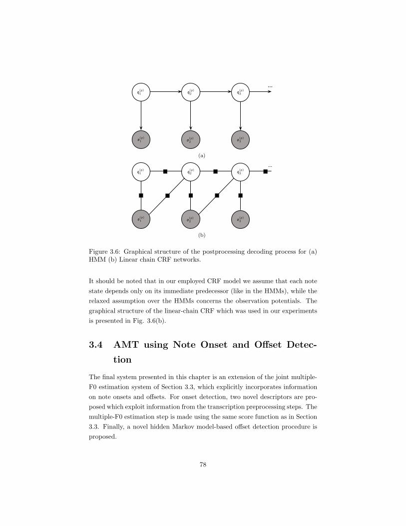
q(p)1 q
(p)2 q
(p)3
o(p)1 o
(p)2 o
(p)3
...
(a)
q(p)1 q
(p)2 q
(p)3
o(p)1 o
(p)2 o
(p)3
...
(b)
Figure 3.6: Graphical structure of the postprocessing decoding process for (a)HMM (b) Linear chain CRF networks.
It should be noted that in our employed CRF model we assume that each note
state depends only on its immediate predecessor (like in the HMMs), while the
relaxed assumption over the HMMs concerns the observation potentials. The
graphical structure of the linear-chain CRF which was used in our experiments
is presented in Fig. 3.6(b).
3.4 AMT using Note Onset and Offset Detec-
tion
The final system presented in this chapter is an extension of the joint multiple-
F0 estimation system of Section 3.3, which explicitly incorporates information
on note onsets and offsets. For onset detection, two novel descriptors are pro-
posed which exploit information from the transcription preprocessing steps. The
multiple-F0 estimation step is made using the same score function as in Section
3.3. Finally, a novel hidden Markov model-based offset detection procedure is
proposed.
78
3.4.1 Preprocessing
Resonator Time-Frequency Image
As in the systems of Sections 3.2 and 3.3, the resonator time-frequency image
was used as a time-frequency representation. The same settings were used, and
the resulting absolute value of the RTFI is denoted as X [ω, t] while an RTFI
slice is denoted as X [ω].
Spectral Whitening and Noise Suppression
In order to suppress timbral information and make the following analysis more
robust to different sound sources, spectral whitening is performed using the same
method described in Section 3.3, resulting in the whitened representation Y [ω, t].
Afterwards, an algorithm for noise suppression is applied to the whitened RTFI,
using the two-stage median filtering procedure presented in subsection 3.3.1.The
result is a whitened and noise-suppressed RTFI representation Z[ω].
Salience Function
Using Z[ω], the log-frequency pitch salience function S[p] proposed in Section
3.2 is extracted, where p ∈ [21, . . . , 108] denotes MIDI pitch. Tuning and in-
harmonicity coefficients are also extracted. Using the extracted information, a
harmonic partial sequence (HPS) HPS [p, h] for each candidate pitch p and its
harmonics h = 1, . . . , 13 is also stored for further processing.
3.4.2 Onset Detection
In order to accurately detect onsets in polyphonic music, two onset descriptors
which exploit information from the transcription preprocessing steps are pro-
posed and combined using late fusion. Firstly, a novel spectral flux-based feature
is defined, which incorporates pitch tuning information. Although spectral flux
has been successfully used in the past for detecting hard onsets [BDA+05], false
alarms may be detected for instruments that produce frequency modulations
such as vibrato or portamento. Thus, a semitone-resolution filterbank is cre-
ated from Z[ω, t], where each filter is centered at the estimated tuning position
of each pitch:
ψ[p, t] =
( ωp,0+δp+4∑
l=ωp,0+δp−4
Z[l, t] ·Wp[l]
) 12
(3.30)
79

where ωp,0 is the bin that ideally corresponds to pitch p and Wp is a 80 cent-
span Hanning window centered at the pitch tuning position. Using the output
of the filterbank, the novel spectral flux-based descriptor is defined as:
SF [t] =
108∑
p=21
HW (ψ[p, t]− ψ[p, t− 1]) (3.31)
where HW (·) = ·+|·|2 is a half-wave rectifier. Afterwards, onsets can be detected
by performing peak picking on SF [t].
In order to detect soft onsets, which may not be indicated by a change in
signal energy [BDA+05], a pitch-based descriptor is proposed which is based on
the extracted salience function. The salience function S[p, t] is smoothed using a
moving median filter with 120 ms span, in order to reduce any fluctuations that
might be attributed to amplitude modulations (e.g. tremolo). The smoothed
salience function S[p, t] is then warped into a chroma-like representation:
Chr [p, t] =6∑
i=0
S[12 · i+ p+ 20, t] (3.32)
where p = 1, . . . , 12 represents the pitch classes C, C♯,. . .,B. Afterwards, the
half-wave rectified first-order difference of Chr [p, t] is used as a pitch-based onset
detection function (denoted as salience difference SD):
SD [t] =
12∑
i=1
HW (Chr[i, t]− Chr[i, t− 1]) (3.33)
Accordingly, soft onsets are detected by peak picking on SD [t].
In order to combine the onsets produced by the two aforementioned descrip-
tors, late fusion is applied, as in [HS10]. From each of the two descriptors an
onset strength signal is created, which contains either the value one at the in-
stant of the detected onset or zero otherwise. The fused onset strength signal
is created by summing and smoothing these two signals using a moving median
filter of 40 ms length. Onsets are detected by performing peak picking on the
fused signal by selecting peaks with a minimum 80 ms distance. For tuning
onset detection parameters, a development set containing ten 30 sec classical
recordings from the meter analysis data from Ghent University [VM07] was
employed.
80

3.4.3 Multiple-F0 Estimation
We perform the same multiple-F0 estimation procedure described in subsection
3.4.3 using segments defined by two consecutive onsets instead of performing
multiple-F0 estimation for each time frame.
Overlapping Partial Treatment
We extract segments defined by two consecutive onsets by using the mean Z[ω, t]
of the first 3 frames after the onset. Using each segment, a salience function
and HPS are extracted. A set of CN candidate pitches is selected, based on
the maximum values of the salience function S[p] (here, CN is set to 10 as in
[EBD10]). The pitch candidate set will be denoted as C.
In order to recover the amplitude of overlapped harmonics, we employ the
proposed discrete cepstrum-based spectral envelope estimation algorithm de-
scribed in subsection 3.3.2 and detailed in Appendix B. Firstly, given a subset
C of pitch candidates, a partial collision list is computed. For a given HPS, if
the number of overlapped partials is less than Nover , then the amplitudes of
the overlapped partials are estimated from the spectral envelope SEp[ω] of the
candidate pitch using only amplitude information from non-overlapped partials.
If the number of overlapped partials is equal or greater than Nover , the partial
amplitudes are estimated using spectral envelope information from the complete
HPS.
Pitch set score function
Having selected a set of possible pitch candidates and performed overlapping
partial treatment on each possible combination, the goal is to select the optimal
pitch combination for a specific time frame. A modified version of the pitch
set score function presented in subsection 3.3.2 is employed, which combines
spectral and temporal characteristics of the candidate F0s, and also attempts
to minimize the noise residual to avoid any missed detections.
Given a candidate pitch set C ⊆ C with size |C|, the proposed pitch set score
function is given by (3.16), where in this case Lp is defined as:
Lp = w1Fl [p] + w2Sm[p]− w3SC [p] + w4PR[p] (3.34)
where Fl [p], Sm[p], SC [p],PR[p] are defined in subsection 3.3.2.
81

In order to train the weight parameters wi, i = 1, . . . , 4 of the features in
(3.34) as well as for the residual weight in (3.17), training was performed using
the Nelder-Mead search algorithm for parameter estimation [NM65] with 100
classic, jazz, and random piano chords from the MAPS database [EBD10] as
a training set. Trained weight parameters wi were 1.3, 1.4, 0.6, 0.5, 25. The
pitch candidate set C that maximizes the score function is selected as the pitch
estimate for the current frame.
3.4.4 Offset Detection
In order to accurately detect note offsets we employ hidden Markov models
(HMMs). HMMs have been used in the past for smoothing transcription results
(e.g. [QRC+10]) but to the author’s knowledge they have not been utilized for
offset detection. As in the note tracking procedure of Subsection 3.3.1, each
pitch is modeled by a two-state HMM, denoting pitch activity/inactivity. The
observation sequence O(p) is given by the output of the multiple-F0 estimation
step for each pitch, while the state sequence is given by Q(p). In order to
estimate state priors P (q(p)1 ) and the state transition matrix P (q
(p)t |q
(p)t−1), MIDI
files from the RWC database [GHNO03] from the classic and jazz genres were
used.
In order to estimate the observation probabilities P (o(p)t |q
(p)t ), we employ a
sigmoid curve which has as input the salience function of an active pitch from
the output of the multiple-F0 estimation step:
P (o(p)t |q
(p)t = 1) =
1
1 + e−(S[p,t]−1)(3.35)
where S[p, t] denotes the salience function value at frame t. The output of the
HMM-based offset detection step is generated using the Viterbi algorithm. The
note offset is detected as the time frame when an active pitch between two
consecutive onsets changes from an active to an inactive state for the first time.
Thus, the main difference between the present system and the system of Section
3.3 in terms of postprocessing is that for each active note event between two
onsets, only one offset must be present; in the system of Section 3.3, a note
event in an “off” state might move to an “on” state in the next frame. Thus,
the present system explicitly models note offsets. An example for the complete
transcription system, from preprocessing to offset detection, is given in Fig. 3.7
for a guitar recording from the RWC database.
82
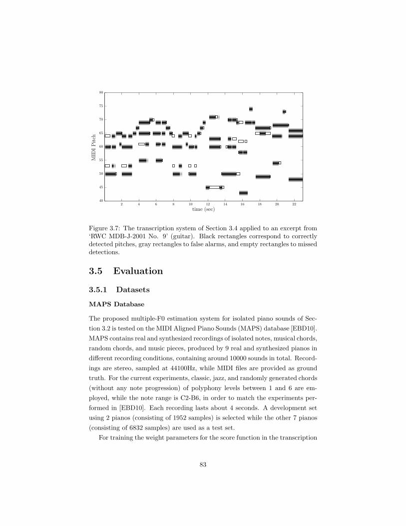
time (sec)
MID
IPitch
2 4 6 8 10 12 14 16 18 20 2240
45
50
55
60
65
70
75
80
Figure 3.7: The transcription system of Section 3.4 applied to an excerpt from‘RWC MDB-J-2001 No. 9’ (guitar). Black rectangles correspond to correctlydetected pitches, gray rectangles to false alarms, and empty rectangles to misseddetections.
3.5 Evaluation
3.5.1 Datasets
MAPS Database
The proposed multiple-F0 estimation system for isolated piano sounds of Sec-
tion 3.2 is tested on the MIDI Aligned Piano Sounds (MAPS) database [EBD10].
MAPS contains real and synthesized recordings of isolated notes, musical chords,
random chords, and music pieces, produced by 9 real and synthesized pianos in
different recording conditions, containing around 10000 sounds in total. Record-
ings are stereo, sampled at 44100Hz, while MIDI files are provided as ground
truth. For the current experiments, classic, jazz, and randomly generated chords
(without any note progression) of polyphony levels between 1 and 6 are em-
ployed, while the note range is C2-B6, in order to match the experiments per-
formed in [EBD10]. Each recording lasts about 4 seconds. A development set
using 2 pianos (consisting of 1952 samples) is selected while the other 7 pianos
(consisting of 6832 samples) are used as a test set.
For training the weight parameters for the score function in the transcription
83

systems of Sections 3.3 and 3.4, samples from the MAPS database are also
used. Here, 103 samples from two piano types are employed for training1.
For comparative experiments on isolated piano sounds using the transcription
system of Section 3.3, it should be noted that the postprocessing stage was not
employed for the MAPS dataset.
RWC Dataset
For the transcription experiments of systems presented in Sections 3.3 and 3.4,
we use 12 excerpts from the RWC database [GHNO03], which have been used
in the past to evaluate polyphonic music transcription approaches in [KNS07,
SKT+08, QRC+10]. A list of the employed recordings along with the instru-
ments present in each one is shown in the top half of Table 3.1. The recordings
containing ‘MDB-J’ in their RWC ID belong to the jazz genre, while those that
contain ‘MDB-C’ belong to the classic genre. For the recording titles and com-
poser, the reader can refer to [SKT+08]. Five additional pieces are also selected
from the RWC database, which have not yet been evaluated in the literature.
These pieces are described in the bottom half of Table 3.1 (data 13-17).
As far as ground-truth for the RWC data 1-12 shown in Table 3.1, non-
aligned MIDI files are provided along with the original 44.1 kHz recordings.
However, these MIDI files contain several note errors and omissions, as well
as unrealistic note durations, thus making them unsuitable for transcription
evaluation. As in [KNS07, SKT+08, QRC+10], aligned ground-truth MIDI data
has been created for the first 23s of each recording, using Sonic Visualiser [Son]
for spectrogram visualization and MIDI editing. For the RWC data 13-17 in
Table 3.1, the newly-released syncRWC ground truth annotations are utilized2.
Disklavier Dataset
The test dataset developed by Poliner and Ellis [PE07a] is also used for tran-
scription experiments. It contains 10 one-minute recordings from a Yamaha
Disklavier grand piano, sampled at 8 kHz. Aligned MIDI ground truth using
the Disklavier is also provided with the recordings. The list of music pieces that
are contained in this dataset is shown in Table 3.2.
1Trained weight parameters for the system of Section 3.3 are wi = 1.3, 1.4, 0.6, 0.5, 0.2, 25.2http://staff.aist.go.jp/m.goto/RWC-MDB/AIST-Annotation/SyncRWC/
84
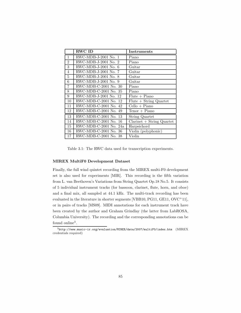
RWC ID Instruments
1 RWC-MDB-J-2001 No. 1 Piano2 RWC-MDB-J-2001 No. 2 Piano3 RWC-MDB-J-2001 No. 6 Guitar4 RWC-MDB-J-2001 No. 7 Guitar5 RWC-MDB-J-2001 No. 8 Guitar6 RWC-MDB-J-2001 No. 9 Guitar7 RWC-MDB-C-2001 No. 30 Piano8 RWC-MDB-C-2001 No. 35 Piano9 RWC-MDB-J-2001 No. 12 Flute + Piano10 RWC-MDB-C-2001 No. 12 Flute + String Quartet11 RWC-MDB-C-2001 No. 42 Cello + Piano12 RWC-MDB-C-2001 No. 49 Tenor + Piano
13 RWC-MDB-C-2001 No. 13 String Quartet14 RWC-MDB-C-2001 No. 16 Clarinet + String Quartet15 RWC-MDB-C-2001 No. 24a Harpsichord16 RWC-MDB-C-2001 No. 36 Violin (polyphonic)17 RWC-MDB-C-2001 No. 38 Violin
Table 3.1: The RWC data used for transcription experiments.
MIREX MultiF0 Development Dataset
Finally, the full wind quintet recording from the MIREX multi-F0 development
set is also used for experiments [MIR]. This recording is the fifth variation
from L. van Beethoven’s Variations from String Quartet Op.18 No.5. It consists
of 5 individual instrument tracks (for bassoon, clarinet, flute, horn, and oboe)
and a final mix, all sampled at 44.1 kHz. The multi-track recording has been
evaluated in the literature in shorter segments [VBB10, PG11, GE11, OVC+11],
or in pairs of tracks [MS09]. MIDI annotations for each instrument track have
been created by the author and Graham Grindlay (the latter from LabROSA,
Columbia University). The recording and the corresponding annotations can be
found online3.
3http://www.music-ir.org/evaluation/MIREX/data/2007/multiF0/index.htm (MIREXcredentials required)
85
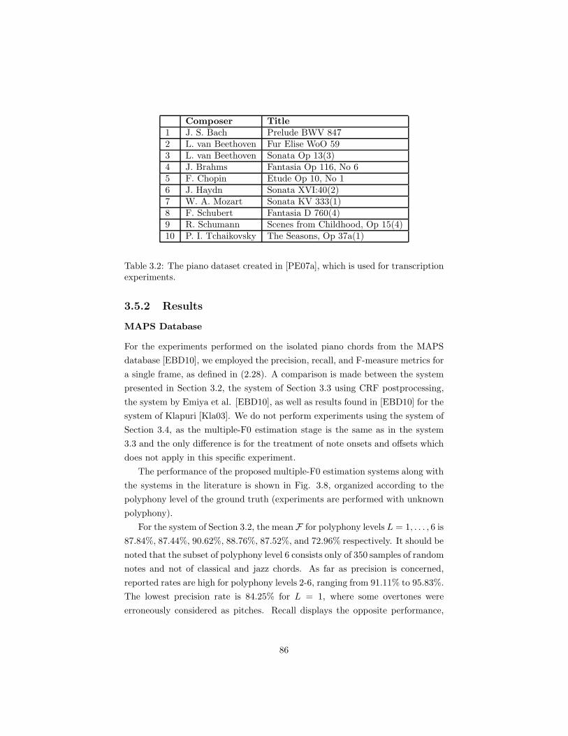
Composer Title
1 J. S. Bach Prelude BWV 8472 L. van Beethoven Fur Elise WoO 593 L. van Beethoven Sonata Op 13(3)4 J. Brahms Fantasia Op 116, No 65 F. Chopin Etude Op 10, No 16 J. Haydn Sonata XVI:40(2)7 W. A. Mozart Sonata KV 333(1)8 F. Schubert Fantasia D 760(4)9 R. Schumann Scenes from Childhood, Op 15(4)10 P. I. Tchaikovsky The Seasons, Op 37a(1)
Table 3.2: The piano dataset created in [PE07a], which is used for transcriptionexperiments.
3.5.2 Results
MAPS Database
For the experiments performed on the isolated piano chords from the MAPS
database [EBD10], we employed the precision, recall, and F-measure metrics for
a single frame, as defined in (2.28). A comparison is made between the system
presented in Section 3.2, the system of Section 3.3 using CRF postprocessing,
the system by Emiya et al. [EBD10], as well as results found in [EBD10] for the
system of Klapuri [Kla03]. We do not perform experiments using the system of
Section 3.4, as the multiple-F0 estimation stage is the same as in the system
3.3 and the only difference is for the treatment of note onsets and offsets which
does not apply in this specific experiment.
The performance of the proposed multiple-F0 estimation systems along with
the systems in the literature is shown in Fig. 3.8, organized according to the
polyphony level of the ground truth (experiments are performed with unknown
polyphony).
For the system of Section 3.2, the mean F for polyphony levels L = 1, . . . , 6 is
87.84%, 87.44%, 90.62%, 88.76%, 87.52%, and 72.96% respectively. It should be
noted that the subset of polyphony level 6 consists only of 350 samples of random
notes and not of classical and jazz chords. As far as precision is concerned,
reported rates are high for polyphony levels 2-6, ranging from 91.11% to 95.83%.
The lowest precision rate is 84.25% for L = 1, where some overtones were
erroneously considered as pitches. Recall displays the opposite performance,
86
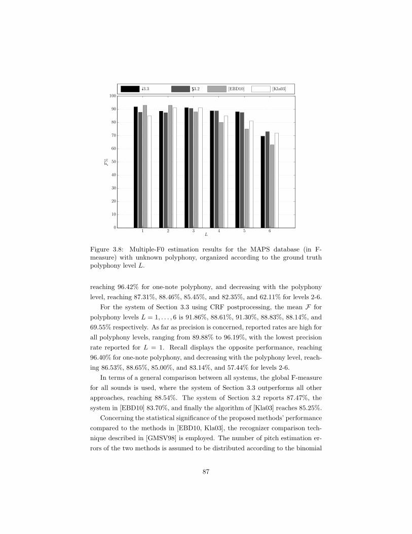
[Kla03][EBD10]§3.2§3.3F%
L1 2 3 4 5 6
0
10
20
30
40
50
60
70
80
90
100
Figure 3.8: Multiple-F0 estimation results for the MAPS database (in F-measure) with unknown polyphony, organized according to the ground truthpolyphony level L.
reaching 96.42% for one-note polyphony, and decreasing with the polyphony
level, reaching 87.31%, 88.46%, 85.45%, and 82.35%, and 62.11% for levels 2-6.
For the system of Section 3.3 using CRF postprocessing, the mean F for
polyphony levels L = 1, . . . , 6 is 91.86%, 88.61%, 91.30%, 88.83%, 88.14%, and
69.55% respectively. As far as precision is concerned, reported rates are high for
all polyphony levels, ranging from 89.88% to 96.19%, with the lowest precision
rate reported for L = 1. Recall displays the opposite performance, reaching
96.40% for one-note polyphony, and decreasing with the polyphony level, reach-
ing 86.53%, 88.65%, 85.00%, and 83.14%, and 57.44% for levels 2-6.
In terms of a general comparison between all systems, the global F-measure
for all sounds is used, where the system of Section 3.3 outperforms all other
approaches, reaching 88.54%. The system of Section 3.2 reports 87.47%, the
system in [EBD10] 83.70%, and finally the algorithm of [Kla03] reaches 85.25%.
Concerning the statistical significance of the proposed methods’ performance
compared to the methods in [EBD10, Kla03], the recognizer comparison tech-
nique described in [GMSV98] is employed. The number of pitch estimation er-
rors of the two methods is assumed to be distributed according to the binomial
87
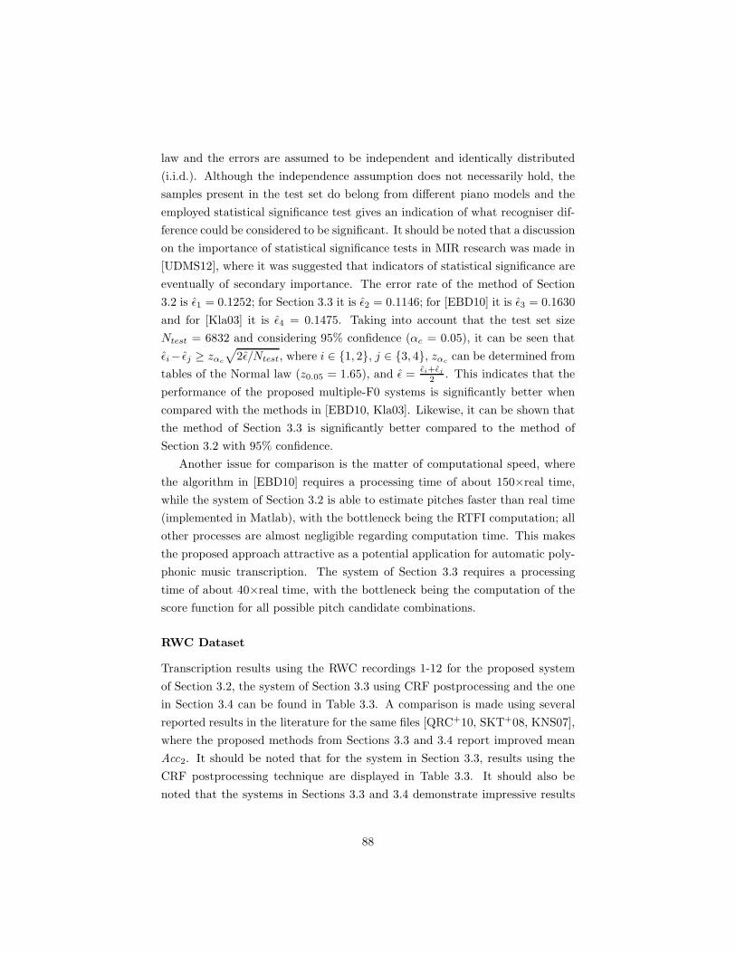
law and the errors are assumed to be independent and identically distributed
(i.i.d.). Although the independence assumption does not necessarily hold, the
samples present in the test set do belong from different piano models and the
employed statistical significance test gives an indication of what recogniser dif-
ference could be considered to be significant. It should be noted that a discussion
on the importance of statistical significance tests in MIR research was made in
[UDMS12], where it was suggested that indicators of statistical significance are
eventually of secondary importance. The error rate of the method of Section
3.2 is ǫ1 = 0.1252; for Section 3.3 it is ǫ2 = 0.1146; for [EBD10] it is ǫ3 = 0.1630
and for [Kla03] it is ǫ4 = 0.1475. Taking into account that the test set size
Ntest = 6832 and considering 95% confidence (αc = 0.05), it can be seen that
ǫi− ǫj ≥ zαc
√2ǫ/Ntest, where i ∈ 1, 2, j ∈ 3, 4, zαc
can be determined from
tables of the Normal law (z0.05 = 1.65), and ǫ =ǫi+ǫj
2 . This indicates that the
performance of the proposed multiple-F0 systems is significantly better when
compared with the methods in [EBD10, Kla03]. Likewise, it can be shown that
the method of Section 3.3 is significantly better compared to the method of
Section 3.2 with 95% confidence.
Another issue for comparison is the matter of computational speed, where
the algorithm in [EBD10] requires a processing time of about 150×real time,
while the system of Section 3.2 is able to estimate pitches faster than real time
(implemented in Matlab), with the bottleneck being the RTFI computation; all
other processes are almost negligible regarding computation time. This makes
the proposed approach attractive as a potential application for automatic poly-
phonic music transcription. The system of Section 3.3 requires a processing
time of about 40×real time, with the bottleneck being the computation of the
score function for all possible pitch candidate combinations.
RWC Dataset
Transcription results using the RWC recordings 1-12 for the proposed system
of Section 3.2, the system of Section 3.3 using CRF postprocessing and the one
in Section 3.4 can be found in Table 3.3. A comparison is made using several
reported results in the literature for the same files [QRC+10, SKT+08, KNS07],
where the proposed methods from Sections 3.3 and 3.4 report improved mean
Acc2. It should be noted that for the system in Section 3.3, results using the
CRF postprocessing technique are displayed in Table 3.3. It should also be
noted that the systems in Sections 3.3 and 3.4 demonstrate impressive results
88
§3.4 §3.3 §3.2 [QRC+10] [SKT+08] [KNS07]1 60.0% 60.2% 61.0% 63.5% 59.0% 64.2%2 73.6% 75.0% 64.9% 72.1% 63.9% 62.2%3 62.5% 57.9% 53.8% 58.6% 51.3% 63.8%4 65.2% 66.8% 51.8% 79.4% 68.1% 77.9%5 53.4% 54.8% 46.3% 55.6% 67.0% 75.2%6 76.1% 74.4% 54.6% 70.3% 77.5% 81.2%7 68.5% 64.0% 62.3% 49.3% 57.0% 70.9%8 60.1% 58.9% 48.4% 64.3% 63.6% 63.2%9 50.3% 53.9% 47.2% 50.6% 44.9% 43.2%10 72.4% 74.1% 66.2% 55.9% 48.9% 48.1%11 56.2% 50.0% 43.0% 51.1% 37.0% 37.6%12 33.0% 35.7% 31.0% 38.0% 35.8% 27.5%
Mean 61.2% 60.5% 52.5% 59.1% 56.2% 59.6%
Std. 11.2% 11.5% 10.2% 11.5% 12.9% 16.9%
Table 3.3: Transcription results (Acc2) for the RWC recordings 1-12.
for some recordings compared to the state-of-the-art (e.g. in file 11, which is
a cello-piano duet) while in other cases they fall behind. In file 4 for example,
results are inferior compared to state-of-the-art, which could be attributed to the
digital effects applied in the recording (the present system was created mostly
for transcribing classical and jazz music). As far as the standard deviation of
the Acc2 metric is concerned, the systems in Sections 3.3 and 3.4 reports 11.5%
and 11.2% respectively, which is comparable to the state-of-the-art approaches
in Table 3.3, although it is worth noting that the lowest standard deviation is
reported for the method of Section 3.2.
For the RWC recordings 13-17, transcription results comparing all proposed
methods from Sections 3.4, 3.3, and 3.2, can be found in Table 3.4. It should be
noted that no results have been published in the literature for these recordings.
In general, it can be seen that bowed string transcriptions are more accurate
than woodwind transcriptions. Compared to RWC recordings 1-12, the system
in Section 3.3 performs better compared to the one in Section 3.4, which can be
attributed to the soft onsets found in the pitched non-percussive sounds found
in recordings 13-17.
Additional insight into the proposed systems’ performance for all 17 RWC
recordings is given in Table 3.5, where the error metrics of Section 2.5 are pre-
sented. Results using three different configurations are shown for the system
of Section 3.3: without any note smoothing, with HMM-based note smoothing,
89

§3.4 §3.3 §3.213 60.3% 48.2% 37.7%14 47.7% 41.8% 41.0%15 57.8% 66.8% 50.6%16 60.1% 70.7% 61.7%17 52.0% 75.2% 58.3%
Mean 55.5% 60.5% 49.9%
Std. 5.5% 14.7% 10.5%
Table 3.4: Transcription results (Acc2) for RWC recordings 13-17.
and with CRF-based note smoothing. For the system of Section 3.4, two differ-
ent configurations are evaluated, using the complete system for onset and offset
detection, as well as a variant of the system performing only onset detection
for each segment defined by two onsets. It can be seen that for the system of
Section 3.3, there is a significant accuracy improvement when a postprocessing
technique is employed. In specific, the note postprocessing procedures mainly
decrease the number of false alarms (as can be seen in Efp), at the expense
however of missed detections (Efn ). Especially for the HMM postprocessing, a
large number of missed detections have impaired the system’s performance.
As for the MAPS dataset, the recognizer comparison technique described
in [GMSV98] was employed. Even though the independence assumption does
not necessarily hold for time frames within a recording, it can be argued that
performing statistical significance tests between multi-pitch detection rates on
entire pieces (as in the MIREX evaluations) is an over-simplification, especially
given that the problem of detecting multiple pitches out of 88 classes makes the
problem space quite big. This is one of the reasons why to the author’s knowl-
edge no statistical significance tests take place in the transcription literature.
Thus, considering 95% confidence, the performance of the transcription system
of Section 3.3 using CRF postprocessing is significantly better when compared
with the methods in [QRC+10, SKT+08, KNS07] and the systems of Sections
3.2 and 3.4 (the latter using both onset and offset detection). It should also
be noted that the significance threshold was only just surpassed when com-
paring the system of Section 3.3 with the method of [KNS07] and the system
in Section 3.4. For the system of Section 3.3, the accuracy improvement of
the CRF postprocessing step over the HMM one is statistically significant with
95% confidence. Specifically, the significance threshold for this experiment was
90

Method Fon Acc1 Acc2 Etot Esubs Efn Efp§3.2 44.1% 50.9% 51.8% 48.2% 7.8% 33.9% 6.5%§3.3 No Post. 33.8% 55.6% 54.5% 45.4% 11.3% 18.5% 15.7%§3.3 HMM Post. 47.1% 58.5% 59.4% 40.5% 4.7% 31.7% 4.1%§3.3 CRF Post. 48.2% 60.3% 60.5% 39.5% 6.0% 25.1% 8.4%§3.4 onset only 46.1% 57.1% 56.9% 43.1% 9.0% 22.2% 11.9%§3.4 onset+offset 51.1% 59.3% 59.6% 40.4% 7.3% 23.5% 9.6%
Table 3.5: Transcription error metrics for the proposed method using RWCrecordings 1-17.
Removed feature none Fl Sm SC PR AM Fl [Res ]Acc2 60.5% 56.3% 59.2% 58.6% 53.5% 59.4% 29.1%
Table 3.6: Transcription results (Acc2) for the RWC recordings 1-12 using themethod in §3.3, when features are removed from the score function (3.17).
found to be 0.72% in terms of the error rate, which is surpassed by the CRF
postprocessing (being 1.1%).
In order to test the contribution of each feature in the pitch set score function
(3.17) to the performance of the transcription system of Section 3.3, experiments
were made on RWC recordings 1-12. For each experiment, the weight wi, i =
1, . . . , 6 in the score function that corresponds to each feature was set to 0.
Results are shown in Table 3.6, where it can clearly be seen that the most
crucial feature is Fl [Res ], which is the residual flatness. For each experiment,
the weight wi, i = 1, . . . , 6 in the score function that corresponds to each feature
was set to 0. Results are shown in Table 3.6, where it can clearly be seen that
the most crucial feature is Fl [Res ], which is the residual flatness.
When testing the contribution of the inharmonicity estimation in the salience
function which is used in all proposed systems, a comparative experiment us-
ing RWC recordings 1-12 took place with the system of Section 3.3 using
CRF postprocessing, where inharmonicity search is disabled. This results in
Acc2 = 59.7%. By employing the statistical significance test of [GMSV98], the
performance improvement when inharmonicity estimation is enabled is signif-
icant with 90% confidence. It should be noted however that the contribution
of the inharmonicity estimation procedure depends on the instrument sources
that are present in the signal. In addition, by disabling the overlapping partial
treatment procedure for the same experiment, it was shown that Acc2 = 38.0%,
with Efp = 20.4%, which indicates that additional false alarms from the over-
91
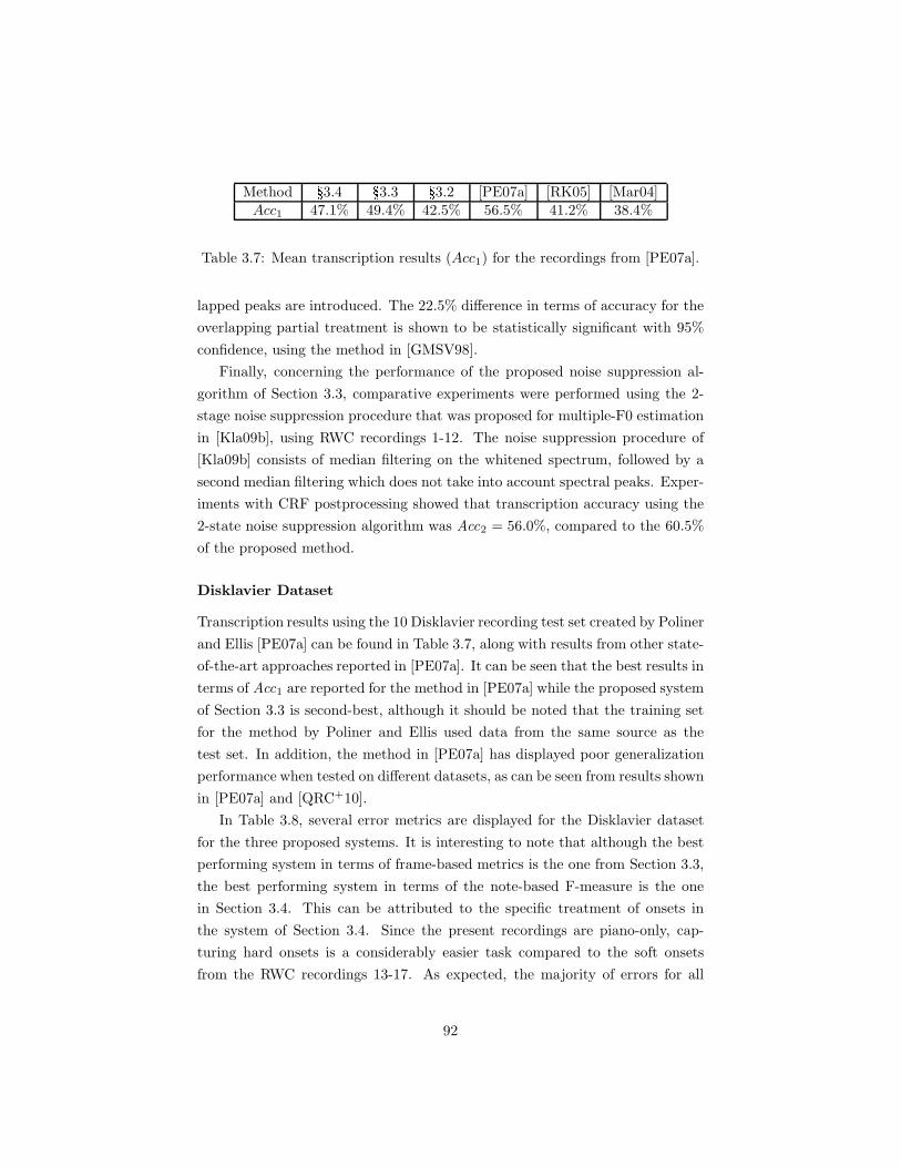
Method §3.4 §3.3 §3.2 [PE07a] [RK05] [Mar04]Acc1 47.1% 49.4% 42.5% 56.5% 41.2% 38.4%
Table 3.7: Mean transcription results (Acc1) for the recordings from [PE07a].
lapped peaks are introduced. The 22.5% difference in terms of accuracy for the
overlapping partial treatment is shown to be statistically significant with 95%
confidence, using the method in [GMSV98].
Finally, concerning the performance of the proposed noise suppression al-
gorithm of Section 3.3, comparative experiments were performed using the 2-
stage noise suppression procedure that was proposed for multiple-F0 estimation
in [Kla09b], using RWC recordings 1-12. The noise suppression procedure of
[Kla09b] consists of median filtering on the whitened spectrum, followed by a
second median filtering which does not take into account spectral peaks. Exper-
iments with CRF postprocessing showed that transcription accuracy using the
2-state noise suppression algorithm was Acc2 = 56.0%, compared to the 60.5%
of the proposed method.
Disklavier Dataset
Transcription results using the 10 Disklavier recording test set created by Poliner
and Ellis [PE07a] can be found in Table 3.7, along with results from other state-
of-the-art approaches reported in [PE07a]. It can be seen that the best results in
terms of Acc1 are reported for the method in [PE07a] while the proposed system
of Section 3.3 is second-best, although it should be noted that the training set
for the method by Poliner and Ellis used data from the same source as the
test set. In addition, the method in [PE07a] has displayed poor generalization
performance when tested on different datasets, as can be seen from results shown
in [PE07a] and [QRC+10].
In Table 3.8, several error metrics are displayed for the Disklavier dataset
for the three proposed systems. It is interesting to note that although the best
performing system in terms of frame-based metrics is the one from Section 3.3,
the best performing system in terms of the note-based F-measure is the one
in Section 3.4. This can be attributed to the specific treatment of onsets in
the system of Section 3.4. Since the present recordings are piano-only, cap-
turing hard onsets is a considerably easier task compared to the soft onsets
from the RWC recordings 13-17. As expected, the majority of errors for all
92
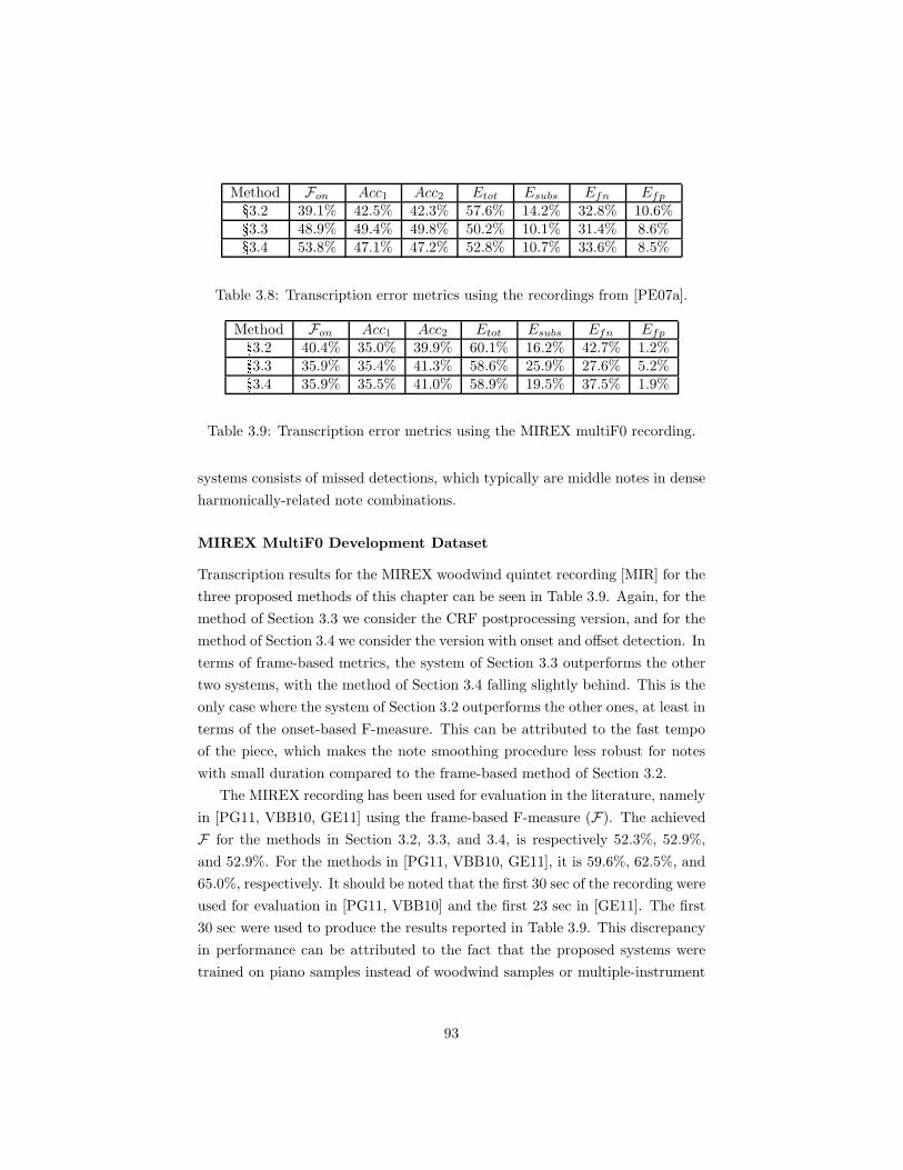
Method Fon Acc1 Acc2 Etot Esubs Efn Efp§3.2 39.1% 42.5% 42.3% 57.6% 14.2% 32.8% 10.6%§3.3 48.9% 49.4% 49.8% 50.2% 10.1% 31.4% 8.6%§3.4 53.8% 47.1% 47.2% 52.8% 10.7% 33.6% 8.5%
Table 3.8: Transcription error metrics using the recordings from [PE07a].
Method Fon Acc1 Acc2 Etot Esubs Efn Efp§3.2 40.4% 35.0% 39.9% 60.1% 16.2% 42.7% 1.2%§3.3 35.9% 35.4% 41.3% 58.6% 25.9% 27.6% 5.2%§3.4 35.9% 35.5% 41.0% 58.9% 19.5% 37.5% 1.9%
Table 3.9: Transcription error metrics using the MIREX multiF0 recording.
systems consists of missed detections, which typically are middle notes in dense
harmonically-related note combinations.
MIREX MultiF0 Development Dataset
Transcription results for the MIREX woodwind quintet recording [MIR] for the
three proposed methods of this chapter can be seen in Table 3.9. Again, for the
method of Section 3.3 we consider the CRF postprocessing version, and for the
method of Section 3.4 we consider the version with onset and offset detection. In
terms of frame-based metrics, the system of Section 3.3 outperforms the other
two systems, with the method of Section 3.4 falling slightly behind. This is the
only case where the system of Section 3.2 outperforms the other ones, at least in
terms of the onset-based F-measure. This can be attributed to the fast tempo
of the piece, which makes the note smoothing procedure less robust for notes
with small duration compared to the frame-based method of Section 3.2.
The MIREX recording has been used for evaluation in the literature, namely
in [PG11, VBB10, GE11] using the frame-based F-measure (F). The achieved
F for the methods in Section 3.2, 3.3, and 3.4, is respectively 52.3%, 52.9%,
and 52.9%. For the methods in [PG11, VBB10, GE11], it is 59.6%, 62.5%, and
65.0%, respectively. It should be noted that the first 30 sec of the recording were
used for evaluation in [PG11, VBB10] and the first 23 sec in [GE11]. The first
30 sec were used to produce the results reported in Table 3.9. This discrepancy
in performance can be attributed to the fact that the proposed systems were
trained on piano samples instead of woodwind samples or multiple-instrument
93
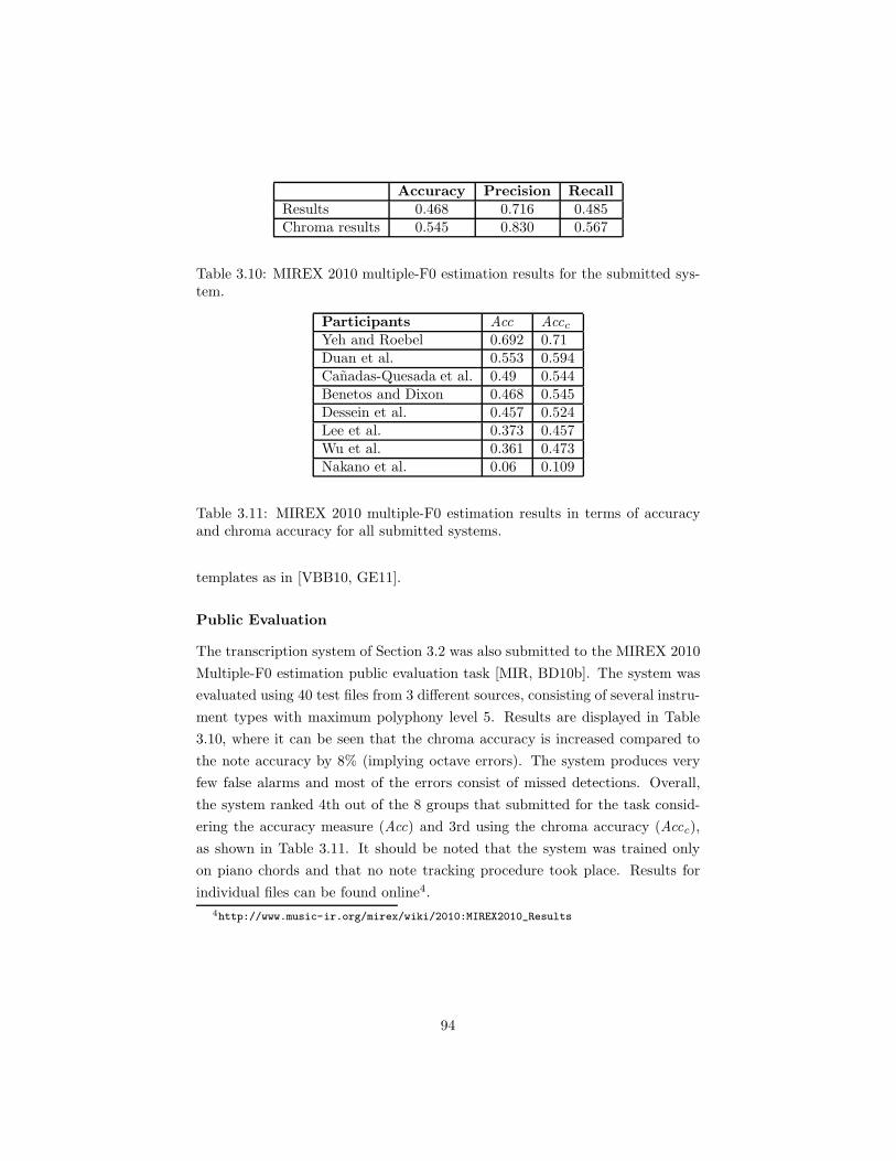
Accuracy Precision Recall
Results 0.468 0.716 0.485Chroma results 0.545 0.830 0.567
Table 3.10: MIREX 2010 multiple-F0 estimation results for the submitted sys-tem.
Participants Acc AcccYeh and Roebel 0.692 0.71Duan et al. 0.553 0.594Canadas-Quesada et al. 0.49 0.544Benetos and Dixon 0.468 0.545Dessein et al. 0.457 0.524Lee et al. 0.373 0.457Wu et al. 0.361 0.473Nakano et al. 0.06 0.109
Table 3.11: MIREX 2010 multiple-F0 estimation results in terms of accuracyand chroma accuracy for all submitted systems.
templates as in [VBB10, GE11].
Public Evaluation
The transcription system of Section 3.2 was also submitted to the MIREX 2010
Multiple-F0 estimation public evaluation task [MIR, BD10b]. The system was
evaluated using 40 test files from 3 different sources, consisting of several instru-
ment types with maximum polyphony level 5. Results are displayed in Table
3.10, where it can be seen that the chroma accuracy is increased compared to
the note accuracy by 8% (implying octave errors). The system produces very
few false alarms and most of the errors consist of missed detections. Overall,
the system ranked 4th out of the 8 groups that submitted for the task consid-
ering the accuracy measure (Acc) and 3rd using the chroma accuracy (Accc),
as shown in Table 3.11. It should be noted that the system was trained only
on piano chords and that no note tracking procedure took place. Results for
individual files can be found online4.
4http://www.music-ir.org/mirex/wiki/2010:MIREX2010_Results
94
3.6 Discussion
This chapter presented several approaches for multiple-F0 estimation and au-
tomatic music transcription based on signal processing-based techniques and
audio features. All proposed systems have been published in international con-
ferences and a journal paper. One system was also publicly evaluated in the
MIREX 2010 contest.
Contributions of this work include a pitch salience function in the log-
frequency domain which supports inharmonicity and tuning changes; audio
features for multiple-F0 estimation which aim to reduce octave errors and to in-
corporate temporal information; a noise suppression algorithm based on a pink
noise assumption; an overlapping partial treatment procedure using a novel har-
monic envelope estimation algorithm; a pitch set score function for joint multi-
pitch estimation; note tracking using conditional random fields; onset detection
incorporating tuning and inharmonicity information; and offset detection using
HMMs.
Multiple-F0 estimation and automatic transcription results showed that pro-
posed systems outperform state-of-the-art algorithms in many cases. Specifi-
cally, the proposed algorithms display robust results in multi-pitch detection of
piano sounds and piano transcription, even in the case where the training and
testing datasets originate from different sources. It was shown that the joint
multiple-F0 estimation algorithm performs better than the iterative multiple-F0
estimation algorithm. Also, in cases where hard onsets were present, explicitly
incorporating note onset information helped in improving results. The main
drawback of a joint multi-pitch detection method is computational complexity.
Finally, it was shown that note smoothing significantly improves transcription
performance.
Although signal processing-based techniques presented in this chapter pro-
vided competitive results with relatively low computational cost, the algorithms
still exhibit a considerable number of missed note detections. Also, expanding
audio feature-based algorithms is not straightforward, since these algorithms
depend on an ever expanding number of sub-modules (e.g. noise suppression,
envelope estimation, score function) that are difficult to isolate and improve.
Moreover, incorporating instrument-specific settings and performing instrument
identification in polyphonic music is not straightforward in audio feature-based
approaches. In order to incorporate more elaborate temporal continuity con-
straints and to support instrument-specific transcription, in the next section we
95

will investigate spectral factorization-based approaches for multi-pitch detec-
tion.
96

Chapter 4
Spectrogram
Factorization-based
Automatic Music
Transcription
4.1 Introduction
This chapter presents methods for automatic music transcription and mono-
phonic pitch estimation using spectrogram factorization techniques. All pro-
posed models are based on probabilistic latent component analysis (PLCA)
[SRS06], which was presented in detail in subsection 2.3.3. PLCA was selected
because it offers a spectrogram factorization model which is easy to generalise
and interpret; thus it can be used for proposing complex models for multiple-
instrument automatic transcription and at the same time to control these mod-
els using temporal or sparsity constraints. The end goal of this chapter is
to build upon PLCA-based approaches for transcription in order to create a
multiple-instrument AMT system which is able to model the temporal evolu-
tion of sounds.
Firstly, a system for automatic music transcription is presented which ex-
tends the shift-invariant PLCA (SI-PLCA) model [SRS08b] for supporting tem-
plates from multiple instrument sources and at the same time to model fre-
97

quency modulations and tuning changes by exploiting shift-invariance in the
log-frequency domain. This model was published in [BD11c, BD12a] and was
publicly evaluated in the MIREX 2011 multiple-F0 estimation and note tracking
task in [BD11b].
Afterwards, a model is proposed for pitch detection which incorporates tem-
poral continuity constraints in order to model the temporal evolution of notes.
The time-frequency representation of a tone is expressed by the model as a
temporal sequence of spectral templates which can also be shifted over log-
frequency. The temporal sequence of the templates is controlled using hidden
Markov models (HMMs) [Rab89]. This model was published in [BD11e].
Finally, a system for multiple-instrument AMT modelling the temporal evo-
lution of sounds is proposed, which is based on the aforementioned models. This
model supports templates for multiple sound states for each note of a set of in-
struments. The order of the sound state templates is controlled using pitch-wise
HMMs. This system was published in [BD12b]. Finally, evaluation results for
pitch detection, multi-pitch detection, and instrument assignment are presented
in this chapter using the proposed spectrogram factorization-based models.
4.2 AMT using a Convolutive Probabilistic Model
The goal of this section is to propose an automatic transcription model which
expands PLCA techniques and is able to support the use of multiple spectral
templates per pitch, as well as per musical instrument. In addition, the model
should also be able to exploit shift-invariance across log-frequency for detect-
ing tuning changes and frequency modulations, unlike other PLCA- and NMF-
based transcription approaches [GE10, DCL10]. Finally, the contribution of
each source should be time- and pitch-dependent, contrary to the relative pitch
tracking method of [MS09]. As in the transcription systems of Chapter 3, note
smoothing is performed using hidden Markov models trained on MIDI data from
the RWC database [GHNO03]. The output of the system is a semitone resolu-
tion pitch activity matrix and a higher resolution time-pitch representation; the
latter can also be used for pitch content visualization purposes. A diagram of
the proposed transcription system can be seen in Fig. 4.1.
98
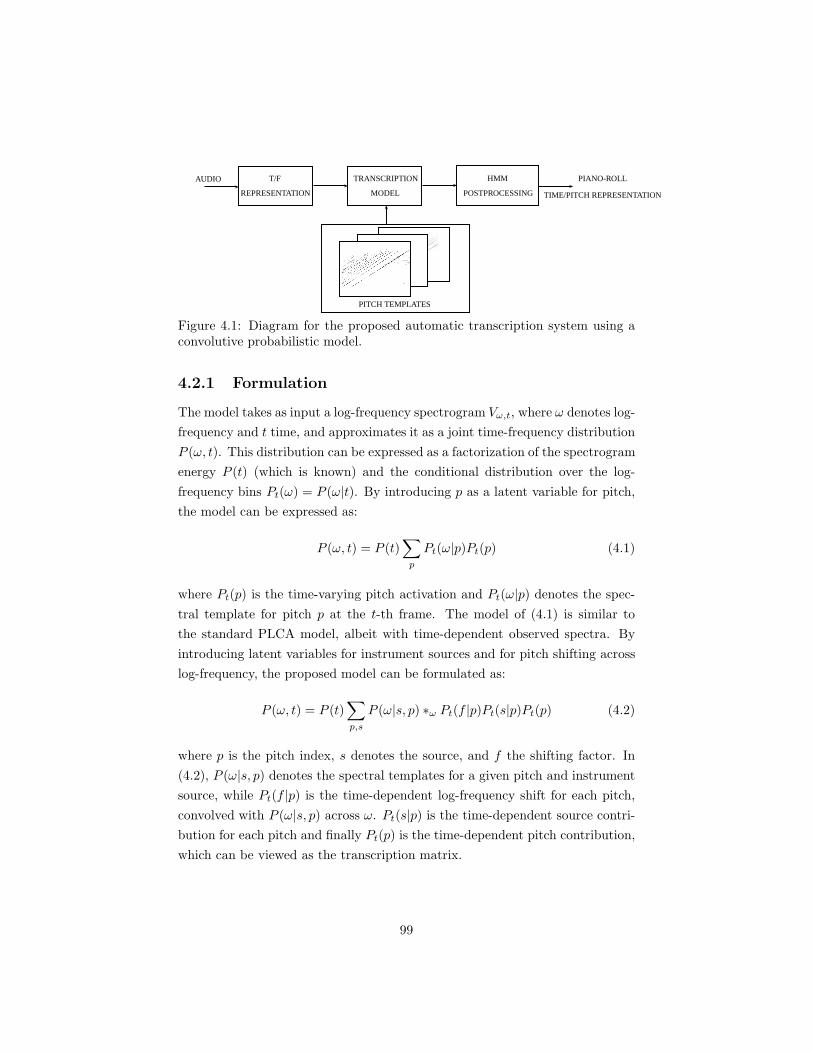
T/F
REPRESENTATION
TRANSCRIPTION
MODEL
HMM
POSTPROCESSING
AUDIO PIANO-ROLL
TIME/PITCH REPRESENTATION
PITCH TEMPLATES
Figure 4.1: Diagram for the proposed automatic transcription system using aconvolutive probabilistic model.
4.2.1 Formulation
The model takes as input a log-frequency spectrogram Vω,t, where ω denotes log-
frequency and t time, and approximates it as a joint time-frequency distribution
P (ω, t). This distribution can be expressed as a factorization of the spectrogram
energy P (t) (which is known) and the conditional distribution over the log-
frequency bins Pt(ω) = P (ω|t). By introducing p as a latent variable for pitch,
the model can be expressed as:
P (ω, t) = P (t)∑
p
Pt(ω|p)Pt(p) (4.1)
where Pt(p) is the time-varying pitch activation and Pt(ω|p) denotes the spec-
tral template for pitch p at the t-th frame. The model of (4.1) is similar to
the standard PLCA model, albeit with time-dependent observed spectra. By
introducing latent variables for instrument sources and for pitch shifting across
log-frequency, the proposed model can be formulated as:
P (ω, t) = P (t)∑
p,s
P (ω|s, p) ∗ω Pt(f |p)Pt(s|p)Pt(p) (4.2)
where p is the pitch index, s denotes the source, and f the shifting factor. In
(4.2), P (ω|s, p) denotes the spectral templates for a given pitch and instrument
source, while Pt(f |p) is the time-dependent log-frequency shift for each pitch,
convolved with P (ω|s, p) across ω. Pt(s|p) is the time-dependent source contri-
bution for each pitch and finally Pt(p) is the time-dependent pitch contribution,
which can be viewed as the transcription matrix.
99

By removing the convolution operator in (4.2), the model becomes:
P (ω, t) = P (t)∑
p,f,s
P (ω − f |s, p)Pt(f |p)Pt(s|p)Pt(p) (4.3)
where P (ω−f |s, p) = P (µ|s, p) denotes the shifted spectral template for a given
pitch and source. It should be noted that as a time-frequency representation,
we employ the constant-Q transform (CQT) with a spectral resolution of 120
bins per octave [SK10]. In order to utilise each spectral template P (ω|s, p) for
detecting a single pitch, we constrain f to a range of one semitone. Thus, f has
a length of 10.
4.2.2 Parameter Estimation
In order to estimate the unknown parameters in the model we employ the
Expectation-Maximization algorithm [DLR77]. Given the input spectrogram
Vω,t, the log-likelihood of the model given the data is:
L =∑
ω,t
Vω,t log(P (ω, t)
)(4.4)
For the Expectation step, we compute the contribution of latent variables
p, f, s over the complete model reconstruction using Bayes’ theorem:
Pt(p, f, s|ω) =P (ω − f |s, p)Pt(f |p)Pt(s|p)Pt(p)∑p,f,s P (ω − f |s, p)Pt(f |p)Pt(s|p)Pt(p)
(4.5)
For the Maximization step, we utilise the posterior of (4.5) for maximizing
the log-likelihood of (4.4), resulting in the following update equations:
P (ω|s, p) =
∑f,t Pt(p, f, s|ω + f)Vω+f,t∑ω,t,f Pt(p, f, s|ω + f)Vω+f,t
(4.6)
Pt(f |p) =
∑ω,s Pt(p, f, s|ω)Vω,t∑f,ω,s Pt(p, f, s|ω)Vω,t
(4.7)
Pt(s|p) =
∑ω,f Pt(p, f, s|ω)Vω,t∑s,ω,f Pt(p, f, s|ω)Vω,t
(4.8)
Pt(p) =
∑ω,f,s Pt(p, f, s|ω)Vω,t∑p,ω,f,s Pt(p, f, s|ω)Vω,t
(4.9)
100

Equations (4.5-4.9) are iterated until convergence (the algorithm is guaranteed
to converge to a local minimum). By keeping the spectral templates P (ω|s, p)
fixed (using pre-extracted templates in a training step), the model converges
quickly, requiring about 10-20 iterations. For the present experiments, we have
set the number of iterations to 15. The runtime for the proposed system is about
50 times real-time. We set p = 1, . . . , 89, where the first 88 indices correspond
to notes A0-C8, and the 89th index corresponds to a residual template (which
is also shifted). The spectral template update rule of eq. (4.6) is applied only
to the 89th template, while all the other pitch templates remain fixed. The
residual template is updated in order to learn the possible noise shape of the
recording, or any other artifacts that might occur in the music signal.
The output of the transcription model is a MIDI-scale pitch activity matrix
and a higher-resolution pitch activation tensor, respectively given by:
P (p, t) = P (t)Pt(p)
P (f, p, t) = P (t)Pt(p)Pt(f |p) (4.10)
By stacking together slices of P (f, p, t) for all pitch values, we can create a
10-cent resolution time-pitch representation:
P (f ′, t) = [P (f, 21, t) · · ·P (f, 108, t)] (4.11)
where f ′ = 1, . . . , 880. The time-pitch representation P (f ′, t) is useful for pitch
content visualization and for the extraction of tuning information.
In Fig. 4.2, the pitch activity matrix P (p, t) for an excerpt of a guitar record-
ing from the RWC database can be seen, along with the corresponding pitch
ground truth. Also, in Fig. 4.3, the time-pitch representation P (f ′, t) of an
excerpt of the ‘RWC MDB-C-2001 No. 12’ (string quartet) recording is shown,
where vibrati in certain notes are visible. It should be noted that these vibrati
would not be captured in a non-shift-invariant model.
4.2.3 Sparsity constraints
Since the proposed model in its unconstrained form is overcomplete (i.e. it con-
tains more information than the input), especially due to the presence of the
convolution operator and its commutativity property, it would be useful to en-
force further constraints in order to regulate the potential increase of information
101
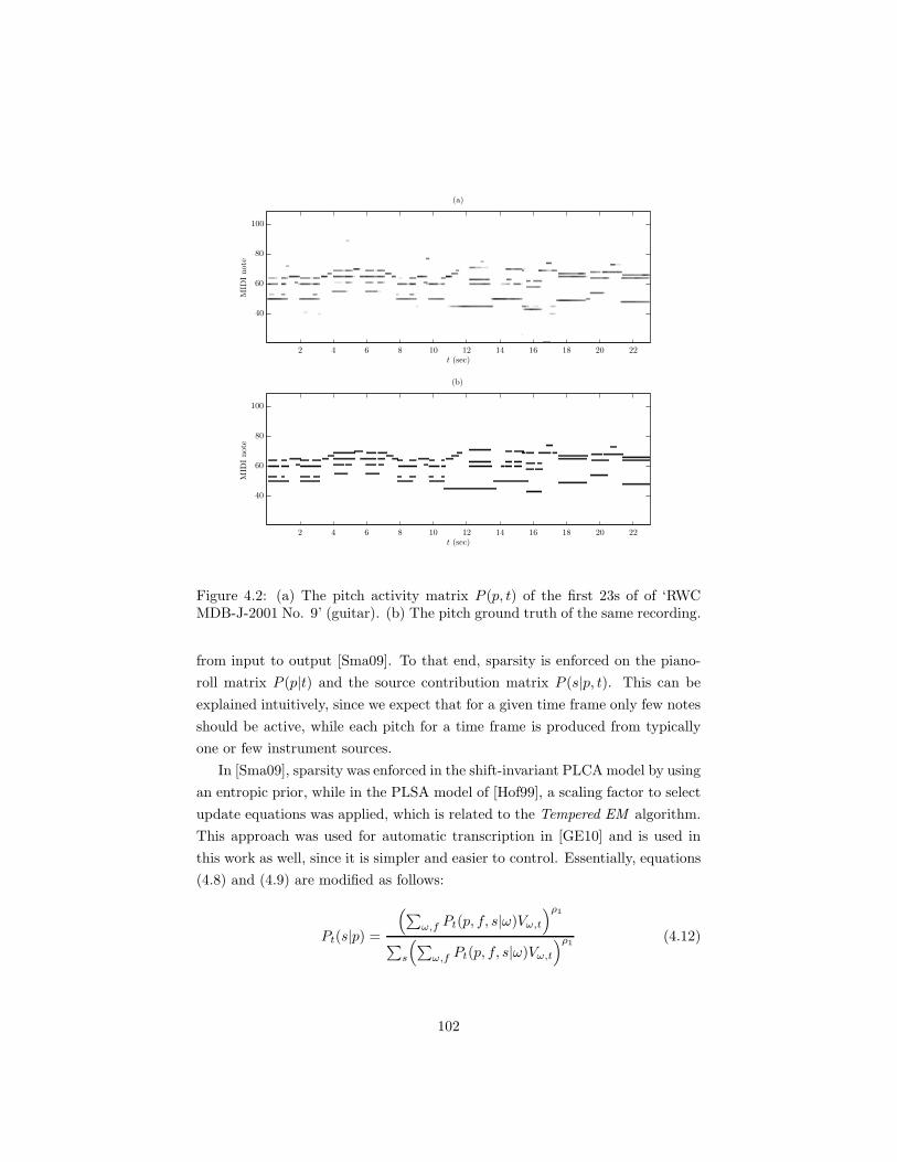
t (sec)
(b)
MID
Inote
t (sec)
(a)
MID
Inote
2 4 6 8 10 12 14 16 18 20 22
2 4 6 8 10 12 14 16 18 20 22
40
60
80
100
40
60
80
100
Figure 4.2: (a) The pitch activity matrix P (p, t) of the first 23s of of ‘RWCMDB-J-2001 No. 9’ (guitar). (b) The pitch ground truth of the same recording.
from input to output [Sma09]. To that end, sparsity is enforced on the piano-
roll matrix P (p|t) and the source contribution matrix P (s|p, t). This can be
explained intuitively, since we expect that for a given time frame only few notes
should be active, while each pitch for a time frame is produced from typically
one or few instrument sources.
In [Sma09], sparsity was enforced in the shift-invariant PLCAmodel by using
an entropic prior, while in the PLSA model of [Hof99], a scaling factor to select
update equations was applied, which is related to the Tempered EM algorithm.
This approach was used for automatic transcription in [GE10] and is used in
this work as well, since it is simpler and easier to control. Essentially, equations
(4.8) and (4.9) are modified as follows:
Pt(s|p) =
(∑ω,f Pt(p, f, s|ω)Vω,t
)ρ1
∑s
(∑ω,f Pt(p, f, s|ω)Vω,t
)ρ1 (4.12)
102
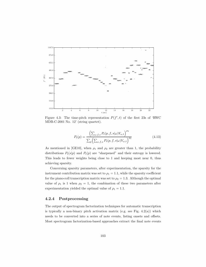
t (sec)
f′(Hz)
2 4 6 8 10 12 14 16 18 20 22
1167.9
874.9
655.5
491.0
367.8
275.6
206.5
154.6
115.9
Figure 4.3: The time-pitch representation P (f ′, t) of the first 23s of ‘RWCMDB-C-2001 No. 12’ (string quartet).
Pt(p) =
(∑ω,f,s Pt(p, f, s|ω)Vω,t
)ρ2
∑p
(∑ω,f,s Pt(p, f, s|ω)Vω,t
)ρ2 (4.13)
As mentioned in [GE10], when ρ1 and ρ2 are greater than 1, the probability
distributions Pt(s|p) and Pt(p) are “sharpened” and their entropy is lowered.
This leads to fewer weights being close to 1 and keeping most near 0, thus
achieving sparsity.
Concerning sparsity parameters, after experimentation, the sparsity for the
instrument contribution matrix was set to ρ1 = 1.1, while the sparsity coefficient
for the piano-roll transcription matrix was set to ρ2 = 1.3. Although the optimal
value of ρ1 is 1 when ρ2 = 1, the combination of these two parameters after
experimentation yielded the optimal value of ρ1 = 1.1.
4.2.4 Postprocessing
The output of spectrogram factorization techniques for automatic transcription
is typically a non-binary pitch activation matrix (e.g. see Fig. 4.2(a)) which
needs to be converted into a series of note events, listing onsets and offsets.
Most spectrogram factorization-based approaches extract the final note events
103

by simply thresholding the pitch activation matrix, e.g. [GE10, DCL10]. As in
the audio feature-based transcription methods of Chapter 3, we employ hidden
Markov models (HMMs) [Rab89] for performing note smoothing and tracking.
Here, we apply note smoothing on the pitch activity matrix P (p, t).
As in Chapter 3, the activity/inactivity of each pitch p is modeled by a
2-state, on/off HMM. MIDI files from the RWC database [GHNO03] from the
classic and jazz genres were employed in order to estimate the pitch-wise state
priors and transition matrices. For estimating the time-varying observation
probability for each active pitch P (o(p)t |q
(p)t = 1), we use a sigmoid curve which
has as input the piano-roll transcription matrix P (p, t):
P (o(p)t |q
(p)t = 1) =
1
1 + e−P (p,t)−λ(4.14)
where λ controls the smoothing as in the postprocessing methods of the previ-
ous chapter. The result of the HMM postprocessing step is a binary piano-roll
transcription which can be used for evaluation. An example of the postprocess-
ing step is given in Fig. 4.4, where the transcription matrix P (p, t) of a piano
recording is seen along with the output of the HMM smoothing.
4.3 Pitch Detection using a Temporally-constrained
Convolutive Probabilistic Model
In this section, a temporally-constrained shift-invariant model for pitch detec-
tion will be presented. The model expresses the evolution of monophonic music
sounds as a sequence of sound state templates, shifted across log-frequency.
The motivation behind it is to address drawbacks of current pitch detection
approaches by: i) explicitly modeling sound states instead of using a constant
spectral template for a complete note event, as in [Sma09, MS09, GE11] and the
system of Section 4.2 ii) incorporating shift-invariance into the model in order to
support the detection of notes which exhibit frequency modulations and tuning
changes, extending the work done in [Mys10, NRK+10]. Finally, compared to
the NMF-based work in [NRK+10], the parameters for the temporal constraints
are learned from a hidden Markov model instead of being pre-defined.
104

t (sec)
MID
Inote
(b)
t (sec)
MID
Inote
(a)
2 4 6 8 10 12 14 16 18 20 22
2 4 6 8 10 12 14 16 18 20 22
30
40
50
60
70
80
90
30
40
50
60
70
80
90
Figure 4.4: (a) The pitch activity matrix P (p, t) of the first 23s of ‘RWC MDB-C-2001 No. 30’ (piano). (b) The piano-roll transcription matrix derived fromthe HMM postprocessing step.
4.3.1 Formulation
The proposed method can be named as HMM-constrained SI-PLCA. The notion
is that the input log-frequency spectrogram1 Vω,t is decomposed as a sum of
sound state spectral templates that are shifted across log-frequency, producing
a pitch track. Each sound state q is constrained using an HMM. Here, ω ∈ [1,Ω]
is the log-frequency index and t ∈ [1, T ] the time index. The model in terms of
the observations is defined as:
P (ω) =∑
q
(P (q1)
∏
t
P (qt+1|qt)
)(∏
t
P (ωt|qt)
)(4.15)
where ω is the complete sequence of draws for all time frames (observable via
Vω,t), q is the sequence of draws of q, P (q1) is the sound state prior distribution,
P (qt+1|qt) is the state transition matrix, P (ωt|qt) is the observation probability
1As in [Mys10], a magnitude spectrogram can be scaled as to yield integer entries.
105
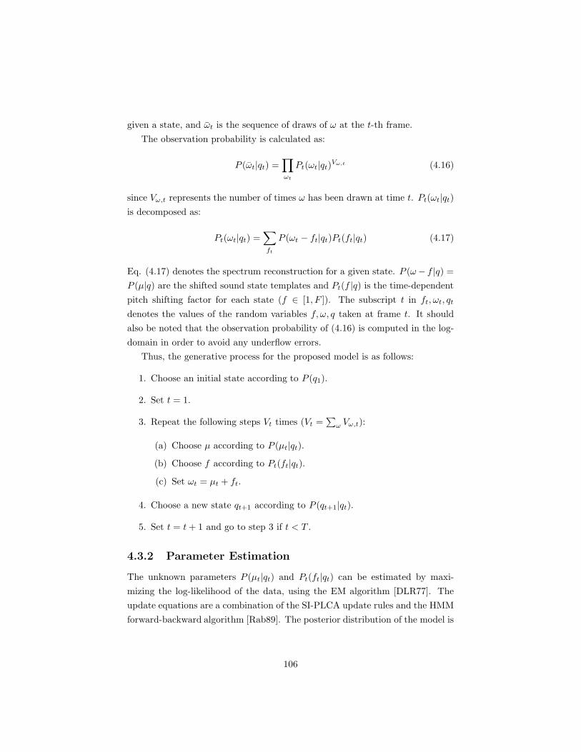
given a state, and ωt is the sequence of draws of ω at the t-th frame.
The observation probability is calculated as:
P (ωt|qt) =∏
ωt
Pt(ωt|qt)Vω,t (4.16)
since Vω,t represents the number of times ω has been drawn at time t. Pt(ωt|qt)
is decomposed as:
Pt(ωt|qt) =∑
ft
P (ωt − ft|qt)Pt(ft|qt) (4.17)
Eq. (4.17) denotes the spectrum reconstruction for a given state. P (ω− f |q) =
P (µ|q) are the shifted sound state templates and Pt(f |q) is the time-dependent
pitch shifting factor for each state (f ∈ [1, F ]). The subscript t in ft, ωt, qt
denotes the values of the random variables f, ω, q taken at frame t. It should
also be noted that the observation probability of (4.16) is computed in the log-
domain in order to avoid any underflow errors.
Thus, the generative process for the proposed model is as follows:
1. Choose an initial state according to P (q1).
2. Set t = 1.
3. Repeat the following steps Vt times (Vt =∑
ω Vω,t):
(a) Choose µ according to P (µt|qt).
(b) Choose f according to Pt(ft|qt).
(c) Set ωt = µt + ft.
4. Choose a new state qt+1 according to P (qt+1|qt).
5. Set t = t+ 1 and go to step 3 if t < T .
4.3.2 Parameter Estimation
The unknown parameters P (µt|qt) and Pt(ft|qt) can be estimated by maxi-
mizing the log-likelihood of the data, using the EM algorithm [DLR77]. The
update equations are a combination of the SI-PLCA update rules and the HMM
forward-backward algorithm [Rab89]. The posterior distribution of the model is
106
given by P (f , q|ω), where f is the sequence of draws of f . Analytical derivations
for the proposed model are presented in Appendix C.
For the Expectation step, we compute the contribution of the latent variables
f, q over the complete model reconstruction:
Pt(ft, qt|ω) =Pt(ft|ω, qt)Pt(ω, qt)
P (ω)= Pt(ft|ωt, qt)Pt(qt|ω) (4.18)
where
Pt(ft|ωt, qt) =P (ωt − ft|qt)Pt(ft|qt)∑ftP (ωt − ft|qt)Pt(ft|qt)
(4.19)
Pt(qt|ω) =Pt(ω, qt)∑qtPt(ω, qt)
=αt(qt)βt(qt)∑qtαt(qt)βt(qt)
(4.20)
Equation (4.18) is the posterior of the hidden variables over the observations
and is computed using the fact that Pt(ft|ω, qt) = Pt(ft|ωt, qt). Equation (4.19)
is computed using Bayes’ rule and the notion that P (ωt|ft, qt) = P (ωt − ft|qt).
Equation (4.20) is the time-varying contribution of each sound state and is
derived from the following:
Pt(ω, qt) = P (ω1, ω2, . . . , ωt, qt)P (ωt+1, ωt+2, . . . , ωT |qt)
= αt(qt)βt(qt) (4.21)
where T is the total number of frames and αt(qt), βt(qt) are the HMM forward
and backward variables [Rab89], respectively.
The forward variable αt(qt) can be computed recursively using the forward-
backward algorithm as follows:
α1(q1) = P (ω1|q1)P (q1)
αt+1(qt+1) =
(∑
qt
P (qt+1|qt)αt(qt)
)·P (ωt+1|qt+1)
(4.22)
while the backward variable βt(qt) can be computed as:
βT (qT ) = 1
βt(qt) =∑
qt+1
βt+1(qt+1)P (qt+1|qt)P (ωt+1|qt+1)
(4.23)
107

The posterior for the sound state transition matrix is given by:
Pt(qt, qt+1|ω) =Pt(ω, qt, qt+1)∑
qt
∑qt+1
Pt(ω, qt, qt+1)=
αt(qt)P (qt+1|qt)βt+1(qt+1)P (ωt+1|qt+1)∑qt,qt+1
αt(qt)P (qt+1|qt)βt+1(qt+1)P (ωt+1|qt+1)(4.24)
For the Maximization step, we derive the update equations for the unknown
parameters P (µ|q), Pt(ft|qt), P (qt+1|qt), and P (q1) using the computed poste-
riors:
P (µ|q) =
∑f,t Vω,tPt(f, q|ω)∑ω,f,t Vω,tPt(f, q|ω)
(4.25)
Pt(ft|qt) =
∑ωtVω,tPt(ft, qt|ω)∑
ft,ωtVω,tPt(ft, qt|ω)
(4.26)
P (qt+1|qt) =
∑t Pt(qt, qt+1|ω)∑
qt+1
∑t Pt(qt, qt+1|ω)
(4.27)
P (q1) = P1(q1|ω) (4.28)
After estimating the unknown parameters, the activation of each sound state is
given by:
Pt(qt|ω)∑
ω
Vω,t (4.29)
An example of the single-source model is given in Fig. 4.5, where the 10-
cent resolution log-frequency spectrogram of a B1 piano note from the MAPS
database [EBD10] is used as input. Here, a 4-state left-to-right HMM is used.
The temporal succession of spectral templates can be seen in Fig. 4.5(d).
4.4 AMT using a Temporally-constrained Con-
volutive Probabilistic Model
In this Section, the single-source model of Section 4.3 is extended for support-
ing multiple sources, as well as multiple components per source. The goal is
to create a multi-pitch detection system for multiple instruments, supporting
also multiple sets of sound state templates per source. At the same time, the
model will be able to support tuning changes and frequency modulations using
a shift-invariant formulation. For modeling the temporal evolution of the sound
state templates, one HMM will be linked with each pitch. Sparsity will also
108
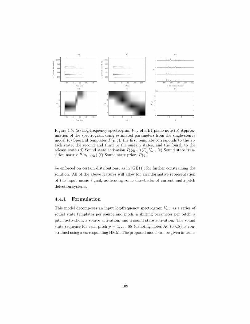
P(q
1)
q
(f)
qt+1
q t
(e)(d)
q
t (40ms hop)
(c)
q
µ (10 cent resolution)
(b)
ω(10centresolution)
t (40ms)
(a)ω(10centresolution)
t (40ms hop)
1 2 3 41 2 3 420 40 60 80 100
200 400 600 800 100020 40 60 80 10020 40 60 80 100
0
0.2
0.4
0.6
0.8
1
1
2
3
4
4
3
2
1
1
2
3
4
200
400
600
800
1000
200
400
600
800
1000
Figure 4.5: (a) Log-frequency spectrogram Vω,t of a B1 piano note (b) Approx-imation of the spectrogram using estimated parameters from the single-sourcemodel (c) Spectral templates P (µ|q); the first template corresponds to the at-tack state, the second and third to the sustain states, and the fourth to therelease state (d) Sound state activation Pt(qt|ω)
∑ω Vω,t (e) Sound state tran-
sition matrix P (qt+1|qt) (f) Sound state priors P (q1)
be enforced on certain distributions, as in [GE11], for further constraining the
solution. All of the above features will allow for an informative representation
of the input music signal, addressing some drawbacks of current multi-pitch
detection systems.
4.4.1 Formulation
This model decomposes an input log-frequency spectrogram Vω,t as a series of
sound state templates per source and pitch, a shifting parameter per pitch, a
pitch activation, a source activation, and a sound state activation. The sound
state sequence for each pitch p = 1, . . . , 88 (denoting notes A0 to C8) is con-
strained using a corresponding HMM. The proposed model can be given in terms
109
of the observations as:
P (ω) =∑
q(1)
· · ·∑
q(88)
P (q(1)1 ) · · ·P (q
(88)1 )
(∏
t
P (q(1)t+1|q
(1)t )
)· · ·
(∏
t
P (q(88)t+1 |q
(88)t )
)
(∏
t
P (ωt|q(1)t , . . . , q
(88)t )
)(4.30)
where q(p) refers to the state sequences for a given pitch, P (q(p)1 ) is the sound
state prior distribution for pitch p, P (q(p)t+1|q
(p)t ) is the sound state transition
matrix, and P (ωt|q(1)t , . . . , q
(88)t ) is the observation probability.
The observation probability is calculated as:
P (ωt|q(1)t , . . . , q
(88)t ) =
∏
ωt
Pt(ωt|q(1)t , . . . , q
(88)t )Vω,t (4.31)
where
Pt(ωt|q(1)t , . . . , q
(88)t ) =
∑
st,pt,ft
Pt(pt)Pt(st|pt)P (ωt − ft|st, pt, q(pt)t )Pt(ft|pt) (4.32)
In (4.32), s denotes the instrument sources, f is the log-frequency pitch shifting
parameter, and q(p) is the sound state sequence linked to pitch p. Pt(p) is
the pitch activity matrix (which is the output of the transcription system),
and Pt(s|p) is the contribution of each instrument source for each pitch across
time. P (ω − f |s, p, q(p)) = P (µ|s, p, q(p)) denotes a spectral template for the
q-th sound state, p-th pitch and s-th source, and Pt(f |p) is the time- and pitch-
dependent log-frequency shifting distribution. For computing (4.32), we exploit
the fact that P (ωt − ft|st, pt, q(1)t , . . . , q
(88)t ) = P (ωt − ft|st, pt, q
(pt)t ). In order
to constrain the pitch shifting f so that each sound state template is associated
with a single pitch, the shifting occurs in a semitone range around the ideal
position of each pitch. Due to memory and computational speed issues, we are
using a log-frequency representation with a spectral resolution of 60 bins per
octave instead of 120 as in the system of Section 4.2. Thus, f ∈ [−2, 2].
Thus, the generative process for the multi-pitch model is as follows:
1. Choose initial states for each p according to P (q(p)1 ).
110

2. Set t = 1.
3. Repeat the following steps Vt times (Vt =∑
ω Vω,t):
(a) Choose p according to Pt(pt).
(b) Choose s according to Pt(st|pt).
(c) Choose f according to Pt(ft|pt).
(d) Choose µ according to P (µt|st, pt, q(pt)t ).
(e) Set ωt = µt + ft.
4. Choose new states q(p)t+1 for each p according to P (q
(p)t+1|q
(p)t ).
5. Set t = t+ 1 and go to step 3 if t < T .
4.4.2 Parameter Estimation
As in Section 4.3, the unknown model parameters can be estimated using the
EM algorithm [DLR77]. For the Expectation step, the posterior of all hidden
variables is given by:
Pt(ft, st, pt, q(1)t , . . . , q
(88)t |ω) =
Pt(q(1)t , . . . , q
(88)t |ω)Pt(ft, st, pt|ωt, q
(1)t , . . . , q
(88)t ) (4.33)
Since we are using independent HMMs, the joint probability of all pitch-wise
sound states over the observations is given by:
Pt(q(1)t , . . . , q
(88)t |ω) =
88∏
p=1
Pt(q(p)t |ω) (4.34)
where
Pt(q(p)t |ω) =
Pt(ω, q(p)t )
∑q(p)t
Pt(ω, q(p)t )
=αt(q
(p)t )βt(q
(p)t )
∑q(p)t
αt(q(p)t )βt(q
(p)t )
(4.35)
and αt(q(p)t ), βt(q
(p)t ) are the forward and backward variables for the p-th HMM
[Rab89], which can be computed recursively using equations (4.22)-(4.23). The
second term of (4.33) can be computed using Bayes’ theorem and the indepen-
111
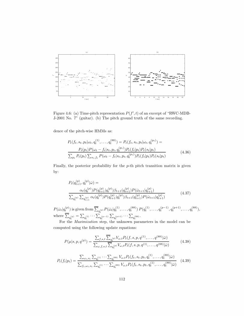
(b)
t (sec)
p
(a)f′
t (sec)2 4 6 8 10 12 14 16 18 20 225 10 15 20
10
20
30
40
50
60
70
80
50
100
150
200
250
300
350
400
Figure 4.6: (a) Time-pitch representation P (f ′, t) of an excerpt of “RWC-MDB-J-2001 No. 7” (guitar). (b) The pitch ground truth of the same recording.
dence of the pitch-wise HMMs as:
Pt(ft, st, pt|ωt, q(1)t , . . . , q
(88)t ) = Pt(ft, st, pt|ωt, q
(pt)t ) =
Pt(pt)P (ωt − ft|st, pt, q(pt)t )Pt(ft|pt)Pt(st|pt)∑
ptPt(pt)
∑st,ft
P (ωt − ft|st, pt, q(pt)t )Pt(ft|pt)Pt(st|pt)
(4.36)
Finally, the posterior probability for the p-th pitch transition matrix is given
by:
Pt(q(p)t+1, q
(p)t |ω) =
αt(q(p)t )P (q
(p)t+1|q
(p)t )βt+1(q
(p)t+1)P (ωt+1|q
(p)t+1)∑
q(p)t
∑q(p)t+1
αt(q(p)t )P (q
(p)t+1|q
(p)t )βt+1(q
(p)t+1)P (ωt+1|q
(p)t+1)
(4.37)
P (ωt|q(p)t ) is given from
∑q(p)t
P (ωt|q(1)t , . . . , q
(88)t ) P (q
(1)t , . . . , q
(p−1)t , q
(p+1)t , . . . , q
(88)t ),
where∑q(p)t
=∑q(1)t
· · ·∑q(p−1)t
∑q(p+1)t
· · ·∑q(88)t
.
For the Maximization step, the unknown parameters in the model can be
computed using the following update equations:
P (µ|s, p, q(p)) =
∑f,s,t
∑q(p)t
Vω,tPt(f, s, p, q(1), . . . , q(88)|ω)
∑ω,f,s,t
∑q(p)t
Vω,tPt(f, s, p, q(1), . . . , q(88)|ω)(4.38)
Pt(ft|pt) =
∑ωt,st
∑q(1)t
· · ·∑q(88)t
Vω,tPt(ft, st, pt, q(1)t , . . . , q
(88)t |ω)
∑ft,ωt,st
∑q(1)t
· · ·∑q(88)t
Vω,tPt(ft, st, pt, q(1)t , . . . , q
(88)t |ω)
(4.39)
112
Pt(st|pt) =
∑ωt,ft
∑q(1)t
· · ·∑
q(88)t
Vω,tPt(ft, st, pt, q(1)t , . . . , q
(88)t |ω)
∑st,ωt,ft
∑q(1)t
· · ·∑q(88)t
Vω,tPt(ft, st, pt, q(1)t , . . . , q
(88)t |ω)
(4.40)
Pt(pt) =
∑ωt,ft,st
∑q(1)t
· · ·∑
q(88)t
Vω,tPt(ft, st, pt, q(1)t , . . . , q
(88)t |ω)
∑pt,ωt,ft,st
∑q(1)t
· · ·∑
q(88)t
Vω,tPt(ft, st, pt, q(1)t , . . . , q
(88)t |ω)
(4.41)
P (q(p)t+1|q
(p)t ) =
∑t Pt(q
(p)t , q
(p)t+1|ω)∑
q(p)t+1
∑t Pt(q
(p)t , q
(p)t+1|ω)
(4.42)
P (q(p)1 ) = P1(q
(p)1 |ω) (4.43)
We should note that the proposed multi-pitch transcription system uses pre-
extracted sound state templates using the single-pitch model of Section 4.3,
thus the spectral template update rule of (4.38) is not utilised, but is included
here for completeness. The runtime for the proposed system is about 100 times
real-time. After convergence using the update equations from the EM steps,
the output of the system is a semitone resolution pitch activity matrix and a
pitch activity tensor in the resolution of the input time-frequency representation,
given respectively by:
Pt(p)∑
ω
Vω,t
Pt(p)Pt(f |p)∑
ω
Vω,t (4.44)
A time-pitch representation can be created by stacking together matrix slices of
tensor Pt(p)Pt(f |p)∑ω Vω,t for all pitch values. We will denote this time-pitch
representation as P (f ′, t), which can be used for pitch visualization purposes
or for extracting tuning information. An example from the proposed model is
given in Fig. 4.6, where the output time-pitch representation P (f ′, t) and the
MIDI ground-truth of a guitar recording can be seen.
4.4.3 Sparsity constraints
The multi-pitch model can be further constrained using sparsity restrictions.
Sparsity was enforced in the shift-invariant models of [Sma09, MS09], using an
entropic prior. However, those models were completely unconstrained, since the
spectral templates were not pre-extracted. Since we know that for a transcrip-
tion problem few notes are active at a given time frame and that few instrument
113

ν2 = 1.2
ν2 = 1.1
ν2 = 1.0L
Iteration0 5 10 15
−5500
−5000
−4500
−4000
−3500
−3000
Figure 4.7: Log-likelihood evolution using different sparsity values for ‘RWC-MDB-J-2001 No.1’ (piano).
sources are responsible for creating a note event at a time frame, we impose
sparsity on the pitch activity matrix Pt(pt) and the pitch-wise source contri-
bution matrix Pt(st|pt). This is achieved in a similar way to [GE10] and the
shift-invariant model in Section 4.2, by modifying update equations (4.40) and
(4.41):
Pt(st|pt) =
(∑ωt,ft,q
(1)t ,...,q
(88)t
Vω,tPt(ft, st, pt, q(1)t , . . . , q
(88)t |ω)
)ρ1
∑st
(∑ωt,ft,q
(1)t ,...,q
(88)t
Vω,tPt(ft, st, pt, q(1)t , . . . , q
(88)t |ω)
)ρ1 (4.45)
Pt(pt) =
(∑ωt,ft,st,q
(1)t ,...,q
(88)t
Vω,tPt(ft, st, pt, q(1)t , . . . , q
(88)t |ω)
)ρ2
∑pt
(∑ωt,ft,st,q
(1)t ,...,q
(88)t
Vω,tPt(ft, st, pt, q(1)t , . . . , q
(88)t |ω)
)ρ2 (4.46)
By setting ρ1, ρ2 > 1, the entropy in matrices Pt(s|p) and Pt(p) is lowered and
sparsity is enforced [GE10]. It should be mentioned that this solution does not
guarantee convergence, although it is observed in practice. In Fig. 4.7, the evo-
lution of log-likelihoodL =∑
ω,t Vω,t log(∑
pt,q(pt)t
Pt(ωt|q(p)t )Pt(q
(pt)t |ω)
∑ω Vω,t
)
can be seen when using different values for sparsity parameter ρ2, for the pi-
ano piece ‘RWC-MDB-J-2001 No.1’. It can be seen that by enforcing sparsity
convergence is still observed, although a higher sparsity value might result in a
worse approximation.
114
4.4.4 Postprocessing
The same postprocessing technique as the one used in subsection 4.2.4 is em-
ployed for the temporally-constrained multi-pitch model. Here, for the pitch-
wise two-state HMMs we use as observations the pitch activation Pt(p)∑
ω Vω,t.
Thus, we define the observation probability for an active note event as:
P (o(p)t |q
(p)t = 1) =
1
1 + e−Pt(p)∑
ωVω,t−λ
(4.47)
As in subsection 4.2.4, eq. (4.47) is a sigmoid curve with Pt(p)∑
ω Vω,t as
input. Parameter λ controls the smoothing (a high value will discard pitch
candidates with low probability). Essentially, in a case of high values in the
pitch activation for a given note, where a gap might occur due to an octave
error, a high self-transition probability in an active state would help filling in
that gap, thus performing note smoothing. The output of the postprocessing
step is a piano-roll transcription, which can be used for evaluation. An example
of the HMM-based note tracking step for the proposed model is given in Fig. 4.8,
where the input pitch activity matrix and the output transcription piano-roll of
a string quartet recording can be seen.
4.5 Evaluation
4.5.1 Training Data
For the transcription systems of Section 4.2, spectral templates are extracted for
various orchestral instruments, using their complete note range. The standard
PLCA model of (2.8) using only one component z is employed in order to extract
a single spectral template. For extracting piano templates, the MAPS database
is employed [EBD10], where templates from three different piano models were
extracted. In addition, note templates are extracted for bassoon, cello, clarinet,
flute, guitar, harpsichord, horn, oboe, pipe organ, and violin using isolated
notes from the RWC musical instrument samples database [GHNO03]. In total,
source parameter s has a size of 13 (3 sets of templates from the piano and 10
for the rest of the instruments). The note range of each instrument used for
sound state template extraction can be seen in Table 4.1. As a time-frequency
representation, the CQT with 120 bins per octave is used [SK10].
For demonstrating the potential of the temporally-constrained pitch detec-
tion system of Section 4.3, sound state templates are extracted for piano, cello,
115
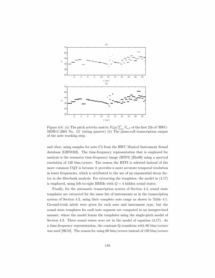
(b)
p
t (sec)
(a)
p
t (sec)
2 4 6 8 10 12 14 16 18 20 22
2 4 6 8 10 12 14 16 18 20 22
20
30
40
50
60
70
20
30
40
50
60
70
Figure 4.8: (a) The pitch activity matrix Pt(p)∑ω Vω,t of the first 23s of ‘RWC-
MDB-C-2001 No. 12’ (string quartet) (b) The piano-roll transcription outputof the note tracking step.
and oboe, using samples for note C4 from the RWC Musical Instrument Sound
database [GHNO03]. The time-frequency representation that is employed for
analysis is the resonator time-frequency image (RTFI) [Zho06] using a spectral
resolution of 120 bins/octave. The reason the RTFI is selected instead of the
more common CQT is because it provides a more accurate temporal resolution
in lower frequencies, which is attributed to the use of an exponential decay fac-
tor in the filterbank analysis. For extracting the templates, the model in (4.17)
is employed, using left-to-right HMMs with Q = 4 hidden sound states.
Finally, for the automatic transcription system of Section 4.4, sound state
templates are extracted for the same list of instruments as in the transcription
system of Section 4.2, using their complete note range as shown in Table 4.1.
Ground-truth labels were given for each note and instrument type, but the
sound state templates for each note segment are computed in an unsupervised
manner, where the model learns the templates using the single-pitch model of
Section 4.3. Three sound states were set in the model of equation (4.17). As
a time-frequency representation, the constant-Q transform with 60 bins/octave
was used [SK10]. The reason for using 60 bins/octave instead of 120 bins/octave
116
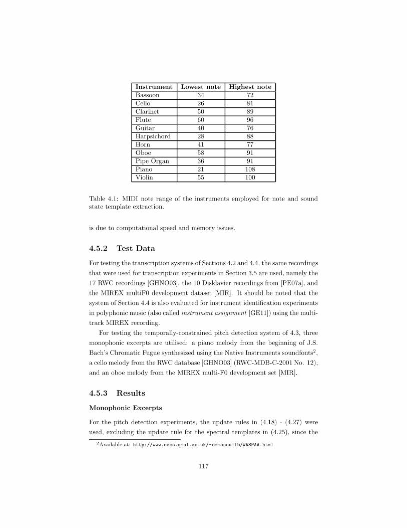
Instrument Lowest note Highest note
Bassoon 34 72Cello 26 81Clarinet 50 89Flute 60 96Guitar 40 76Harpsichord 28 88Horn 41 77Oboe 58 91Pipe Organ 36 91Piano 21 108Violin 55 100
Table 4.1: MIDI note range of the instruments employed for note and soundstate template extraction.
is due to computational speed and memory issues.
4.5.2 Test Data
For testing the transcription systems of Sections 4.2 and 4.4, the same recordings
that were used for transcription experiments in Section 3.5 are used, namely the
17 RWC recordings [GHNO03], the 10 Disklavier recordings from [PE07a], and
the MIREX multiF0 development dataset [MIR]. It should be noted that the
system of Section 4.4 is also evaluated for instrument identification experiments
in polyphonic music (also called instrument assignment [GE11]) using the multi-
track MIREX recording.
For testing the temporally-constrained pitch detection system of 4.3, three
monophonic excerpts are utilised: a piano melody from the beginning of J.S.
Bach’s Chromatic Fugue synthesized using the Native Instruments soundfonts2,
a cello melody from the RWC database [GHNO03] (RWC-MDB-C-2001 No. 12),
and an oboe melody from the MIREX multi-F0 development set [MIR].
4.5.3 Results
Monophonic Excerpts
For the pitch detection experiments, the update rules in (4.18) - (4.27) were
used, excluding the update rule for the spectral templates in (4.25), since the
2Available at: http://www.eecs.qmul.ac.uk/~emmanouilb/WASPAA.html
117
patterns for each sound state were considered fixed. The detected pitch for the
recordings is summed from the pitch distribution for each sound state:
∑
qt
Pt(qt|ω)Pt(f |qt)∑
ω
Vω,t (4.48)
Using the detected pitch track, a piano-roll representation was created by
summing every 10 pitch bins (which make for one semitone). The output piano-
roll representation was compared against existing MIDI ground truth for the
employed recordings. In Fig. 4.9, an excerpt of the employed piano melody
can be seen along with the weighted sound state transitions using the employed
model with a left-to-right HMM. For each tone, the transition from the attack
state to two sustain states, followed by a brief decay state can clearly be seen.
For evaluation, the frame-based transcription metrics presented in Section 2.5
are utilised, namely the overall accuracy (Acc), the total error (Etot ), the sub-
stitution error (Esubs), missed detection error (Efn ), and false alarm error (Efp).
For comparative purposes, the shift-invariant PLCA method in [Sma09] is also
employed for transcription. In this case, one spectral template per source is
employed, using the same training data as in the proposed method.
Pitch detection results using the proposed model are displayed for each
recording in Table 4.2. Experiments using the proposed method are performed
using left-to-right and ergodic HMMs (where all possible transitions between
states were allowed). Although the use of an ergodic model might not be
ideal in cases where the sound evolves clearly between the attack, transient,
sustain, and decay states, it might be useful for instruments where different
sustain states alternate (e.g. tremolo). It can be seen that in all cases, the pro-
posed temporally-constrained convolutive model outperforms the shift-invariant
PLCA method in terms of overall transcription accuracy. Also, the accuracy is
relatively high for the piano and cello recordings, but significantly lower for the
oboe recording. This can be attributed to the fact that the spectral pattern of
oboe notes is not constant for all pitches, but in fact changes drastically. Most
of the missed detections are located in the decay states of tones, whereas most
false alarms are octave errors occurring in the attack part of notes. Finally,
when comparing the HMM topologies, it can be seen that the ergodic model
slightly outperforms the left-to-right one.
118

t (sec)
q
(b)
ω
(a)
0.5 1 1.5 2
0.5 1 1.5 2
100
200
300
400
500
600
700
800
900
1000
4
3
2
1
Figure 4.9: (a) Log-frequency spectrogram of a segment of the piano melodyemployed for experiments (b) Weighted state transitions Pt(qt|ω)
∑ω Vω,t.
RWC Dataset
Transcription results using the 12 excerpts from the RWC database [GHNO03]
are shown in terms of Acc2 in Table 4.3, for the polyphonic transcription meth-
ods presented in this chapter. Comparisons are also made with the proposed au-
dio feature-based methods of Chapter 3. It should be noted that for the method
of Section 4.2, the input T/F representation has a resolution of 120 bins/octave,
while for the method of Section 4.4, the resolution is 60 bins/octave. For the
latter case, this was done due to computational speed and memory purposes,
since the system supports sound state templates for multiple pitches and instru-
ments. From Table 4.3, it can clearly be seen that the proposed spectrogram
factorization methods outperform the proposed audio feature-based methods.
In addition, all proposed methods outperform state-of-the-art results for the
same dataset, for the GMM-based method of [QRC+10], the specmurt method
of [SKT+08], and the HTC method of [KNS07] (detailed results for the afore-
mentioned methods can be seen in Table 3.3).
In terms of specific recordings, the lowest performance of all systems is re-
ported for recording 12, which is a piano-tenor duet. On the other hand, the best
119

Method Instrument Acc Etot Esubs Efn Efp§4.3(LtR)
Piano 81.5% 17.8% 2.2% 9.8% 5.8%Cello 80.3% 22.1% 8.3% 5.6% 15.7%Oboe 55.0% 39.1% 13.3% 22.6% 3.2%§4.3
(ergodic)
Piano 82.2% 16.9% 2.2% 9.5% 5.2%Cello 80.5% 22.2% 5.6% 5.4% 16.2%Oboe 55.6% 37.5% 14.9% 19.3% 3.2%
SI-PLCAPiano 80.1% 20.2% 1.6% 10.7% 7.9%Cello 75.0% 28.5% 1.2% 9.2% 18.0%Oboe 54.1% 41.9% 13.7% 20.5% 7.7%
Table 4.2: Pitch detection results using the proposed method of Section 4.3 withleft-to-right and ergodic HMMs, compared with the SI-PLCA method.
performance for the spectrogram factorization systems is reported for record-
ing 10, which was performed by a string quartet. This demonstrates that this
method can well support the transcription of recordings of non-ideally tuned
instruments which also exhibit vibrati, which is not as well supported by signal
processing-based methods. In addition, results using RWC recordings 13-17,
which have not been evaluated by other methods in the literature, can be seen
in Table 4.4. Again, the temporally-constrained system outperforms all other
proposed systems.
Additional transcription metrics for RWC recordings 1-17 using the system
of Section 4.4 along with two variants of the system of Section 4.2 (with a
frequency resolution of 60 and 120 bins per octave) can be seen in Table 4.5. By
comparing the two systems with a frequency resolution of 60 bins per octave, it
can be seen that incorporating temporal constraints for the evolution of notes
significantly improves transcription accuracy. Octave errors counting as note
substitutions have been diminished in the temporally-constrained system due
to modeling the decay state of tones, where in some cases the higher harmonics
might be suppressed (e.g. piano). It can also be seen that a greater spectral
resolution helps improve performance. In all three cases, the most common
errors occurring in the system are missed detections, usually occurring in dense
chords, where only the root note is detected and the higher notes are considered
as harmonics. Another source of missed detections in the frame-based evaluation
also occurs when the decay part of a note is not recognised due to low energy.
Given the fact that estimating note durations is a challenging task even for
a human annotator, missed detections due to different note durations are not
considered as serious as e.g. octave errors. Note substitutions can also be
120
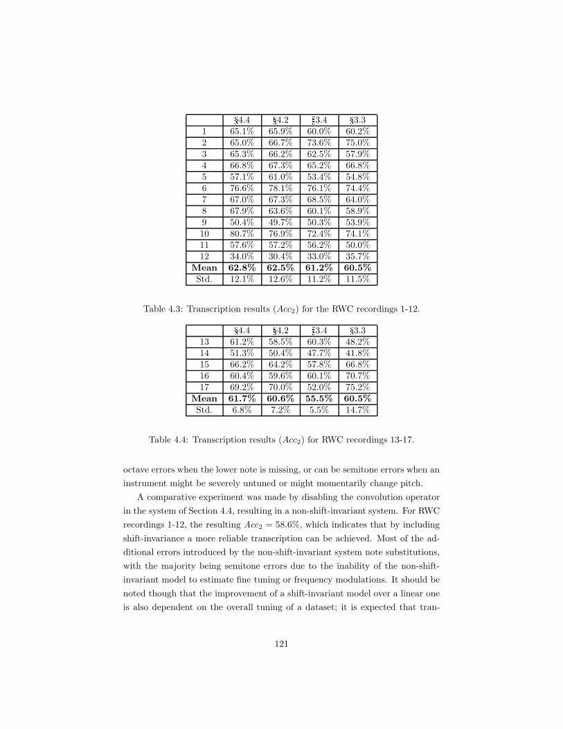
§4.4 §4.2 §3.4 §3.31 65.1% 65.9% 60.0% 60.2%2 65.0% 66.7% 73.6% 75.0%3 65.3% 66.2% 62.5% 57.9%4 66.8% 67.3% 65.2% 66.8%5 57.1% 61.0% 53.4% 54.8%6 76.6% 78.1% 76.1% 74.4%7 67.0% 67.3% 68.5% 64.0%8 67.9% 63.6% 60.1% 58.9%9 50.4% 49.7% 50.3% 53.9%10 80.7% 76.9% 72.4% 74.1%11 57.6% 57.2% 56.2% 50.0%12 34.0% 30.4% 33.0% 35.7%
Mean 62.8% 62.5% 61.2% 60.5%
Std. 12.1% 12.6% 11.2% 11.5%
Table 4.3: Transcription results (Acc2) for the RWC recordings 1-12.§4.4 §4.2 §3.4 §3.313 61.2% 58.5% 60.3% 48.2%14 51.3% 50.4% 47.7% 41.8%15 66.2% 64.2% 57.8% 66.8%16 60.4% 59.6% 60.1% 70.7%17 69.2% 70.0% 52.0% 75.2%
Mean 61.7% 60.6% 55.5% 60.5%
Std. 6.8% 7.2% 5.5% 14.7%
Table 4.4: Transcription results (Acc2) for RWC recordings 13-17.
octave errors when the lower note is missing, or can be semitone errors when an
instrument might be severely untuned or might momentarily change pitch.
A comparative experiment was made by disabling the convolution operator
in the system of Section 4.4, resulting in a non-shift-invariant system. For RWC
recordings 1-12, the resulting Acc2 = 58.6%, which indicates that by including
shift-invariance a more reliable transcription can be achieved. Most of the ad-
ditional errors introduced by the non-shift-invariant system note substitutions,
with the majority being semitone errors due to the inability of the non-shift-
invariant model to estimate fine tuning or frequency modulations. It should be
noted though that the improvement of a shift-invariant model over a linear one
is also dependent on the overall tuning of a dataset; it is expected that tran-
121

Method Fon Acc1 Acc2 Etot Esubs Efn Efp§4.4 60 bins/octave 47.7% 62.0% 62.5% 37.5% 7.8% 19.4% 10.2%§4.2 60 bins/octave 46.8% 60.4% 60.2% 39.8% 9.3% 16.7% 13.8%§4.2 120 bins/octave 47.0% 61.3% 61.9% 38.1% 8.4% 19.0% 10.6%
Table 4.5: Transcription error metrics for the proposed methods using RWCrecordings 1-17.
scribing an untuned dataset will cause additional errors in a non-shift-invariant
transcription model.
In order to test the effect of the HMM-based postprocessing step, a compar-
ative experiment is made which replaces the smoothing procedure with simple
thresholding on the pitch activity matrix P (p, t). Using the set of 12 RWC
recordings, the best result for the system of Section 4.2 is Acc2 = 61.9%, which
is 0.7% worse compared to the HMM postprocessing step. For the system of Sec-
tion 4.4, Acc2 = 61.9%, which again shows that the HMM-based postprocessing
helps achieve improved performance compared to simple thresholding.
Regarding sparsity parameters ρ1 and ρ2, the accuracy rates for the RWC
recordings 1-12 using different sparsity values for the two parameters are pre-
sented in Figs. 4.10 and 4.11 for systems of Sections 4.2 and 4.4 respectively. It
can be seen that with increased source contribution sparsity the accuracy of the
system diminishes, while enforcing sparsity on the pitch activation leads to a
significant improvement. However, after experimentation the optimal combina-
tion of sparsity parameters was found to be ρ1 = 1.1 and ρ2 = 1.4 for the system
of Section 4.4, due to the interaction between parameters. For the system of
Section 4.2 the combination of sparsity parameters was found to be ρ1 = 1.1
and ρ2 = 1.3.
Concerning the statistical significance of the accuracy improvement of the
proposed system compared to the other reported systems from the literature,
the same recogniser comparison technique of [GMSV98] that was used in Chap-
ter 3 was used. For the experiments using the RWC dataset, the significance
threshold with 95% confidence is 0.72% in terms of Acc2, which makes the
improvement significant for the spectrogram factorization-based systems com-
pared to the audio feature-based systems. Although the 0.3% improvement for
the temporally-constrained system of Section 4.4 over the system of Section 4.2
is not significant, the inclusion of the temporal constraints using the same T/F
representation is actually significant, as can be seen from Table 4.5.
122

ρ1
ρ2
parameter value
Acc
2(%
)
1.0 1.1 1.2 1.3 1.4 1.550
55
60
65
Figure 4.10: Transcription results (Acc2) for the system of Section 4.2 for RWCrecordings 1-12 using various sparsity parameters (while the other parameter isset to 1.0).
Method §4.4 60 b/o §4.2 120 b/o §4.2 60 b/o [PE07a] [RK05]Acc1 58.2% 58.9% 57.6% 56.5% 41.2%
Table 4.6: Mean transcription results (Acc1 ) for the piano recordings from[PE07a].
Disklavier Dataset
Transcription results using the Disklavier dataset from [PE07a] are presented
in Table 4.6. For that case, the proposed spectrogram factorization systems of
Sections 4.2 and 4.4 utilised only the sets of piano templates extracted from
the MAPS database [EBD10]. It can be seen that both proposed spectrogram
factorization-based systems outperform the methods in [PE07a] and [RK05], as
well as the proposed audio feature-based methods (results shown in Table 3.7).
The best accuracy is reported for the system of Section 4.2 with a CQT of 120
bins/octave, although the temporally-constrained system still outperforms the
non-temporally-constrained system with the same CQT resolution.
Additional metrics for the Disklavier dataset are presented in Table 4.7,
where a similar trend can be seen when using the note-based F-measure for the
proposed spectrogram factorization-based systems. Another experiment using
the Disklavier dataset was reported for the sparse coding system of [LYC11]
123
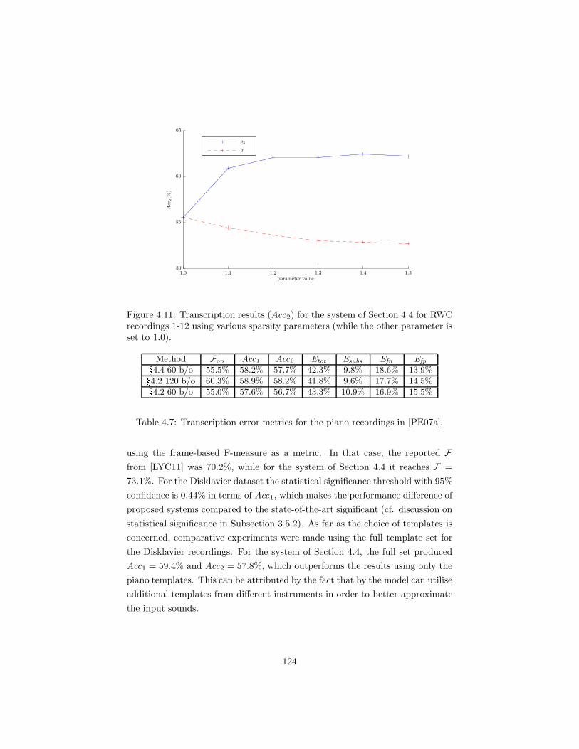
ρ1
ρ2
parameter value
Acc
2(%
)
1.0 1.1 1.2 1.3 1.4 1.550
55
60
65
Figure 4.11: Transcription results (Acc2) for the system of Section 4.4 for RWCrecordings 1-12 using various sparsity parameters (while the other parameter isset to 1.0).
Method Fon Acc1 Acc2 Etot Esubs Efn Efp§4.4 60 b/o 55.5% 58.2% 57.7% 42.3% 9.8% 18.6% 13.9%§4.2 120 b/o 60.3% 58.9% 58.2% 41.8% 9.6% 17.7% 14.5%§4.2 60 b/o 55.0% 57.6% 56.7% 43.3% 10.9% 16.9% 15.5%
Table 4.7: Transcription error metrics for the piano recordings in [PE07a].
using the frame-based F-measure as a metric. In that case, the reported F
from [LYC11] was 70.2%, while for the system of Section 4.4 it reaches F =
73.1%. For the Disklavier dataset the statistical significance threshold with 95%
confidence is 0.44% in terms of Acc1, which makes the performance difference of
proposed systems compared to the state-of-the-art significant (cf. discussion on
statistical significance in Subsection 3.5.2). As far as the choice of templates is
concerned, comparative experiments were made using the full template set for
the Disklavier recordings. For the system of Section 4.4, the full set produced
Acc1 = 59.4% and Acc2 = 57.8%, which outperforms the results using only the
piano templates. This can be attributed by the fact that by the model can utilise
additional templates from different instruments in order to better approximate
the input sounds.
124

Method §4.4 60 b/o §4.2 120 b/o §4.2 60 b/o [PG11] [VBB10]F 65.9% 60.5% 63.7% 59.6% 62.5%
Table 4.8: Frame-based F for the first 30 sec of the MIREX woodwind quintet,comparing the proposed methods with other approaches.
MIREX MultiF0 Development Dataset
Results using the MIREX 2007 woodwind quintet recording are shown in Tables
4.8 and 4.9. In Table 4.8, results using the first 30 sec of the recording are
reported using the frame-based F-measure, compared with the harmonic NMF
method of [VBB10], and the likelihood search method using a Poisson process
in [PG11]. The proposed method of Section 4.4 outperforms other methods
in the literature, including the non-temporally-constrained proposed method
of Section 4.2. It should be noted that the corresponding precision and recall
for the system of Section 4.4 are Pre = 63.7% and Rec = 68.7%. Perhaps
surprisingly, the system of Section 4.2 with 60 bins per octave outperforms the
same system with a CQT of 120 bins per octave, which can be attributed to
convergence issues due to the larger matrix sizes.
Experiments using the MIREX recording were also made in [GE11], where
the authors employed the first 23 sec of the piece and reached an F-measure of
65.0%. Using the first 23 sec of the MIREX recording, the system of Section
4.4 reaches F = 65.8%. It should be noted that additional results are reported
in [GE11] when the eigeninstrument matrices that are employed in that model
are initialised to their optimal values, which are not directly comparable to the
unsupervised experiments in the present work.
Additional transcription metrics for the proposed spectrogram factorization
systems using the complete 54 sec recording are shown in Table 4.9. From
these metrics it can clearly be seen that the proposed spectrogram factorization
systems outperform the proposed audio feature-based systems, for which results
can be seen in Table 3.8. A similar trend as with the RWC dataset can be seen,
where the number of missed detections is significantly greater than the number
of false alarms.
In addition, the first 30 sec of the piece were also utilised in [OVC+11],
resulting in Fn = 66.9%. However, in the case of [OVC+11] the number of
instruments present in the signal is known in advance, making again the ex-
perimental procedure not directly comparable with the present one. It should
125

Method Fn Acc1 Acc2 Etot Esubs Efn Efp§4.4 60 b/o 58.4% 47.8% 51.5% 48.5% 23.7% 12.7% 12.2%§4.2 120 b/o 51.3% 42.2% 47.1% 52.8% 27.6% 13.5% 11.6%§4.2 60 b/o 57.3% 45.2% 50.9% 49.2% 18.5% 25.7% 5.0%
Table 4.9: Transcription error metrics for the complete MIREX woodwind quin-tet.
be noted that for the MIREX quintet Fn is much higher than the frame-based
accuracy measures, while the opposite occurs for the RWC database. This can
be attributed to the fact that the majority of the tones in the MIREX recording
are flute trills (with extremely short duration) that are successfully detected by
the system.
Finally, as far as the choice of templates is concerned, we also transcribe the
MIREX recording using only woodwind templates in the temporally-constrained
system of Section 4.4. The frame-based F-measure reaches 65.2%, which is
about 1% lower compared to the full set of templates. This indicates that
having a large set of templates that might include instruments not present in
the recording does in fact improve transcription accuracy, since the combination
of different instrument templates might better approximate the spectra of the
tones.
Instrument Assignment
An evaluation on the performance of the systems in Sections 4.2 and 4.4 for
instrument identification in polyphonic music is also performed, using the first
30 sec of the MIREX woodwind quintet recording. In this instrument assign-
ment task, a pitch is only considered correct if it occurs at the correct time
and is assigned to the proper instrument source [GE11]. Two variants of the
system are utilised, one using templates from the instruments that are present
in the signal (bassoon, clarinet, flute, horn, and oboe) and another using the
complete set of instrument templates. The instrument-specific output is given
by P (s = i, p, t) = Pt(p)Pt(s = i|p)∑
ω Vω,t, where i is the index for the se-
lected instrument. Postprocessing using the HMM-based methods described in
Sections 4.2 and 4.4 is applied to each instrument-pitch activation in order to
produce a binary piano-roll, which is compared to the MIDI ground truth of the
specific instrument track.
Results for the non-temporally-constrained system of Section 4.2 are pre-
126

Full Set
Woodwinds
F%
Bassoon Clarinet Flute Horn Oboe Mean0
10
20
30
40
50
60
70
Figure 4.12: Instrument assignment results (F) for the method of Section 4.2using the first 30 sec of the MIREX woodwind quintet.
sented in Fig. 4.12, while results for the temporally-constrained system of Sec-
tion 4.4 are presented in Fig. 4.13. It can be seen that the temporally-constrained
system outperforms the non-temporally-constrained one for instrument assign-
ment, for both variants of the system. In the case of the temporally-constrained
system, using the complete set of templates has a higher instrument identifica-
tion accuracy compared to the system that uses only woodwind templates (a
similar trend was reported in [GE11]). This can be attributed to the fact that
combining several instrument templates can help in better approximating tones.
In both systems, clarinet and flute are more accurately transcribed compared
to the rest of the instruments, which might be attributed to the spectral shape
of the clarinet templates and the pitch range of the flute (where the specific
flute notes in the recording were mostly outside the pitch range of the other
woodwind instruments).
The same segment was also evaluated in [OVC+11] where F = 37.0% in
the case where the instrument sources are known. A 22 sec segment of the
same recording was also evaluated in [GE11], where for the proposed system
the F-measure using the woodwind templates is 43.85% and rises to 45.49%
for the complete template set. For the method in [GE11], the reported F-
measure for the complete set of templates was 40.0% and the performance for
127

Full Set
Woodwinds
F%
Bassoon Clarinet Flute Horn Oboe Mean0
10
20
30
40
50
60
70
Figure 4.13: Instrument assignment results (F) for the method of Section 4.4using the first 30 sec of the MIREX woodwind quintet.
the instrument-specific transcription case drops to 35.0%. Thus, the proposed
systems show promising results for instrument assignment in polyphonic music.
Public Evaluation
The transcription system of Section 4.2 was submitted to the MIREX 2011
Multiple-F0 estimation and Note Tracking public evaluation task [MIR, BD11b],
using an input T/F representation of 60 bins/octave, for computational speed
purposes. As in the MIREX 2010 evaluation for the system of Section 3.2, the
evaluation was made using 40 test files from 3 different sources, consisting of sev-
eral instrument types with maximum polyphony level 5. Results for individual
files can be found online3.
Multiple-F0 estimation results are displayed in Table 4.10, where it can
be seen that the chroma accuracy is 5.5% greater than the frame-based pitch
accuracy. The precision and recall of the system are fairly balanced compared
to the system of Section 3.2. Overall, the system ranked 3rd out of the 5 groups
that submitted for the Multiple-F0 estimation task, as shown in Table 4.11.
Compared to the public evaluation of the system of Section 3.2 however, there
3http://www.music-ir.org/mirex/wiki/2011:MIREX2011_Results
128
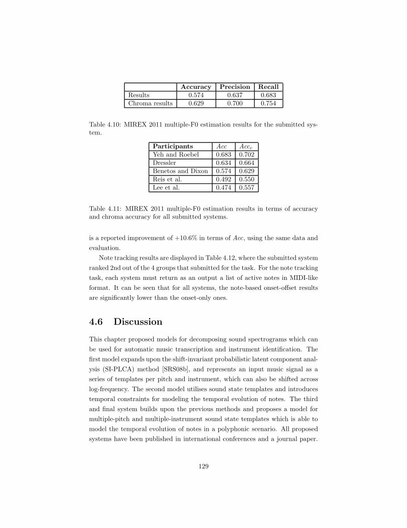
Accuracy Precision Recall
Results 0.574 0.637 0.683Chroma results 0.629 0.700 0.754
Table 4.10: MIREX 2011 multiple-F0 estimation results for the submitted sys-tem.
Participants Acc AcccYeh and Roebel 0.683 0.702Dressler 0.634 0.664Benetos and Dixon 0.574 0.629Reis et al. 0.492 0.550Lee et al. 0.474 0.557
Table 4.11: MIREX 2011 multiple-F0 estimation results in terms of accuracyand chroma accuracy for all submitted systems.
is a reported improvement of +10.6% in terms of Acc, using the same data and
evaluation.
Note tracking results are displayed in Table 4.12, where the submitted system
ranked 2nd out of the 4 groups that submitted for the task. For the note tracking
task, each system must return as an output a list of active notes in MIDI-like
format. It can be seen that for all systems, the note-based onset-offset results
are significantly lower than the onset-only ones.
4.6 Discussion
This chapter proposed models for decomposing sound spectrograms which can
be used for automatic music transcription and instrument identification. The
first model expands upon the shift-invariant probabilistic latent component anal-
ysis (SI-PLCA) method [SRS08b], and represents an input music signal as a
series of templates per pitch and instrument, which can also be shifted across
log-frequency. The second model utilises sound state templates and introduces
temporal constraints for modeling the temporal evolution of notes. The third
and final system builds upon the previous methods and proposes a model for
multiple-pitch and multiple-instrument sound state templates which is able to
model the temporal evolution of notes in a polyphonic scenario. All proposed
systems have been published in international conferences and a journal paper.
129
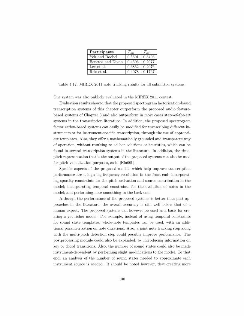
Participants Fon FofYeh and Roebel 0.5601 0.3493Benetos and Dixon 0.4506 0.2077Lee et al. 0.3862 0.2076Reis et al. 0.4078 0.1767
Table 4.12: MIREX 2011 note tracking results for all submitted systems.
One system was also publicly evaluated in the MIREX 2011 contest.
Evaluation results showed that the proposed spectrogram factorization-based
transcription systems of this chapter outperform the proposed audio feature-
based systems of Chapter 3 and also outperform in most cases state-of-the-art
systems in the transcription literature. In addition, the proposed spectrogram
factorization-based systems can easily be modified for transcribing different in-
struments or for instrument-specific transcription, through the use of appropri-
ate templates. Also, they offer a mathematically grounded and transparent way
of operation, without resulting to ad hoc solutions or heuristics, which can be
found in several transcription systems in the literature. In addition, the time-
pitch representation that is the output of the proposed systems can also be used
for pitch visualization purposes, as in [Kla09b].
Specific aspects of the proposed models which help improve transcription
performance are a high log-frequency resolution in the front-end; incorporat-
ing sparsity constraints for the pitch activation and source contribution in the
model; incorporating temporal constraints for the evolution of notes in the
model; and performing note smoothing in the back-end.
Although the performance of the proposed systems is better than past ap-
proaches in the literature, the overall accuracy is still well below that of a
human expert. The proposed systems can however be used as a basis for cre-
ating a yet richer model. For example, instead of using temporal constraints
for sound state templates, whole-note templates can be used, with an addi-
tional parametrisation on note durations. Also, a joint note tracking step along
with the multi-pitch detection step could possibly improve performance. The
postprocessing module could also be expanded, by introducing information on
key or chord transitions. Also, the number of sound states could also be made
instrument-dependent by performing slight modifications to the model. To that
end, an analysis of the number of sound states needed to approximate each
instrument source is needed. It should be noted however, that creating more
130
complex models also signifies the need to introduce additional constraints in
order to control the convergence of the model. Also, computational speed is an-
other issue, especially in convolutive models; to that end, sparse representations
(e.g. [LYC12, ONP12]) can be used, substituting for the EM algorithm.
As far as instrument identification in polyphonic music is concerned, al-
though results outperformed the state-of-the-art for the same experiment, addi-
tional work needs to be done in order to improve the current instrument recog-
nition performance of the proposed systems. This can be achieved by utilizing
the information provided by the source contribution matrix Pt(s|p), combined
with features for characterising music timbre [Pee04].
131
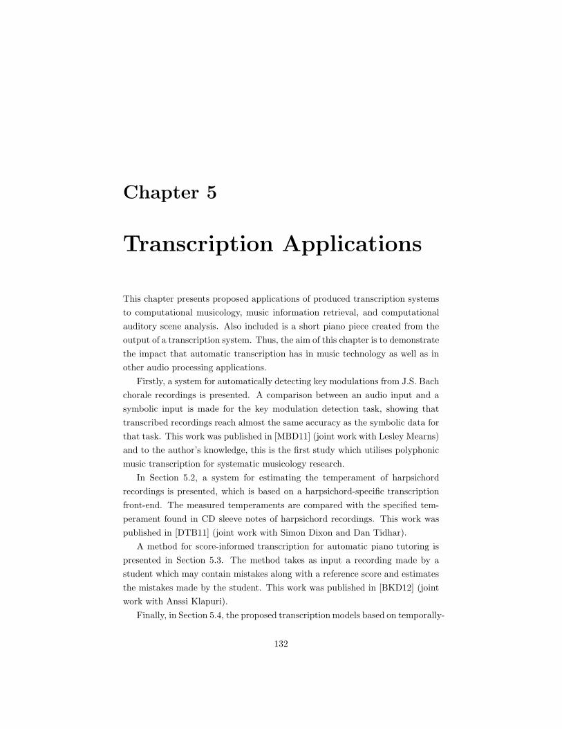
Chapter 5
Transcription Applications
This chapter presents proposed applications of produced transcription systems
to computational musicology, music information retrieval, and computational
auditory scene analysis. Also included is a short piano piece created from the
output of a transcription system. Thus, the aim of this chapter is to demonstrate
the impact that automatic transcription has in music technology as well as in
other audio processing applications.
Firstly, a system for automatically detecting key modulations from J.S. Bach
chorale recordings is presented. A comparison between an audio input and a
symbolic input is made for the key modulation detection task, showing that
transcribed recordings reach almost the same accuracy as the symbolic data for
that task. This work was published in [MBD11] (joint work with Lesley Mearns)
and to the author’s knowledge, this is the first study which utilises polyphonic
music transcription for systematic musicology research.
In Section 5.2, a system for estimating the temperament of harpsichord
recordings is presented, which is based on a harpsichord-specific transcription
front-end. The measured temperaments are compared with the specified tem-
perament found in CD sleeve notes of harpsichord recordings. This work was
published in [DTB11] (joint work with Simon Dixon and Dan Tidhar).
A method for score-informed transcription for automatic piano tutoring is
presented in Section 5.3. The method takes as input a recording made by a
student which may contain mistakes along with a reference score and estimates
the mistakes made by the student. This work was published in [BKD12] (joint
work with Anssi Klapuri).
Finally, in Section 5.4, the proposed transcription models based on temporally-
132
AUDIO TRANSCRIPTIONCHORD
RECOGNITION
KEY
DETECTIONKEY
MODULATIONS
Figure 5.1: Key modulation detection diagram.
constrained shift-invariant probabilistic latent component analysis presented in
Chapter 4 are utilised in the context of computational auditory scene analysis
[WE06], specifically for the characterization of acoustic scenes in train station
recordings. This work was published in [BLD12] (joint work with Mathieu La-
grange).
5.1 Automatic Detection of Key Modulations in
J.S. Bach Chorales
In this section, experiments for the automatic detection of key modulations in
J.S. Bach chorale recordings are presented. Transcribed audio is processed into
vertical notegroups, and the groups are automatically assigned chord labels. For
comparison, MIDI representations of the chorales are also processed. HMMs are
used to detect key change in the chord sequences, based upon two approaches
to chord and key transition representations. The initial hypothesis is that key
and chord values which are derived from pre-eminent music theory will produce
the most accurate models of key and modulation. The music theory models are
tested against models resulting from perceptual experiments about chords and
harmonic relations. Experiments show that the music theory models produce
better results than the perceptual data. The transcribed audio gives encouraging
results, with the key detection outputs ranging from 79% to 97% of the MIDI
ground truth results. The diagram for the proposed key modulation detection
system can be seen in Fig. 5.1.
It should be noted that for this work the author contributed in the collection
of the dataset, the transcription experiments using the proposed system, and
the implementation of the HMMs for key detection.
5.1.1 Motivation
The aims of this work are to test the possibility of obtaining musicological
information directly from audio, which if successful, has the potential to open
up new opportunities for musicological research based on musical recordings,
133

BWV Title
1 1.6 Wie schon leuchtet der Morgenstern2 2.6 Ach Gott, vom Himmel sieh’ darein3 40.6 Schwing dich auf zu deinem Gott4 57.8 Hast du denn, Liebster, dein Angesicht ganzlich verborgen5 85.6 Ist Gott mein Schild und Helfersmann6 140.7 Wachet auf, ruft uns die Stimme7 253 Danket dem Herrn heut und allzeit8 271 Herzlich tut mich verlangen9 359 Jesu meiner Seelen Wonne10 360 Jesu, meiner Freuden Freude11 414 Danket dem Herrn, heut und allzeit12 436 Wie schon leuchtet der Morgenstern
Table 5.1: The list of J.S. Bach chorales used for the key modulation detectionexperiments.
and to ascertain whether perceptual or music theory data is more effective in
the modelling of harmony. To the author’s knowledge, this is the first study
which utilises AMT for systematic musicology research. Although key detection
could also be achieved using an audio-based chord or key detection system,
thus skipping the transcription step, we claim that fully transcribing audio is
appropriate, as it provides a framework for extracting information from a music
piece that is not limited to a specific music information retrieval (MIR) task.
5.1.2 Music Transcription
12 J.S. Bach chorales are randomly selected for experiments from www.jsbchorales.net,
which provides organ-synthesized recordings along with aligned MIDI reference
files. The list of the chorales employed for the key detection experiments can
be seen in Table 5.1. Sample excerpts of original and transcribed chorales are
available online1.
Firstly, the chorale recordings are transcribed into MIDI files using a modi-
fied version of the automatic transcription system of Section 3.4, which is based
on joint multiple-F0 estimation and note onset/offset detection. Since the appli-
cation of the transcription system concerns chorale recordings, the pitch range
was limited to C2-A#6 and the maximum polyphony level was restricted to 4
voices. Since the recordings are synthesized, tempo is constant and it can be
computed using the onset detection functions from Section 3.4. The estimated
pitches in the time frames between two beats are averaged, resulting in a series
1http://www.eecs.qmul.ac.uk/~emmanouilb/chorales.html
134

t (sec)
MID
Ipitch
(a)
t (sec)
MID
Ipitch
(b)
5 10 15 20 25 30 35 40
5 10 15 20 25 30 35 40
70
60
50
40
30
70
60
50
40
30
Figure 5.2: (a) The pitch ground-truth of BWV 2.6 ‘Ach Gott, vom Himmelsieh’ darein’. (b) The transcription output of the same recording.
of chords per beat. Transcription accuracy is 33.1% using the Acc2 metric. An
example of the transcription output of BWV 2.6 ‘Ach Gott, vom Himmel sieh’
darein’ is given in Fig. 5.2.
5.1.3 Chord Recognition
Transcribed audio, and for comparison, ground truth MIDI files, are segmented
into a series of vertical notegroups according to onset times. The algorithm,
which was proposed by Lesley Mearns, can be seen in detail in [MBD11].
To measure the competence of the chord labelling process, the automatically
generated chord sequences are compared to hand annotated sequences. Due to
the laboriousness of hand annotation, six files in the set have been annotated
with ground truth chord sequences (annotations done by Lesley Mearns). It
should be noted that all 12 recordings were annotated for key modulations.
Each pair of chord index values in the sequences is compared, and a basic differ-
ence measure is calculated by counting the number of matches. The final counts
are normalised, resulting in a proportional measure of matched or mismatched
values between the two files (Table 5.2). If two index values differ, the Leven-
shtein distance is calculated for the two pitch class sets represented as strings, to
135

Transcribed Audio Ground Truth Midi
Match Levenshtein Match Levenshtein
0.56 0.64 0.85 0.15
Table 5.2: Chord match results for the six transcribed audio and ground truthMIDI against hand annotations.
find out the degree of difference between the pitch class sets. The Levenshtein
distances calculated for each file are summed and normalised by the length of
sequence to produce a combined measure of accuracy and distance.
A greater quantity of label mismatches are found with the transcribed files
than the ground truth MIDI files, depicting some of the pitch and timing errors
resulting from the automatic transcription. Total chord mismatches between the
transcribed data and the hand annotated data (i.e. where there are no pitches
in common between the two pitch class sets), indicate an error in timing or
quantisation. The greatest difficulty posed to the chord recognition algorithm by
the transcribed data however is the frequent presence of diads rather than triads
in the groups. The transcription algorithm has a low false alarm error rate and
a high missed detection rate, consequently the transcription process produces
an output which assists the chord recognition method where the MIDI data
poses problems; groups with suspended 9th and 13th notes, or other notegroups
containing complex chord tones which are not defined in the chord dictionary,
are captured from the transcribed data as simple triads whereas the MIDI data
may result in a ‘no chord’ value. Complex chords such as 9ths and 13ths are less
adaptable to the pitch class set match approach due to the fact that internal
tones must be omitted from such chords to fit with four part harmony. Overall,
the average accuracy levels for the ground truth files are in the upper range of
accuracy results reported in [PB02]. The transcribed audio achieves an average
of 65% correct of the ground truth result.
5.1.4 Key Modulation Detection
Key change detection is performed using a set of HMMs [Rab89]. The obser-
vation sequence O = ot, t = 1, . . . , T is given by the output of the chord
recognition algorithm in the previous section. The observation matrix therefore
defines the likelihood of a key given a chord. Likewise, the hidden state sequence
which represents keys is given by Q = qt. Each HMM has a key transition
matrix P (qt|qt−1) of size 24×24, (representing the 12 major and 12 minor keys)
136

which defines the probability of making a transition from one key to another.
For a given chord sequence, the most likely key sequence is given by:
Q = argmaxq
∏
t
P (qt|qt−1)P (ot|qt) (5.1)
which can be estimated using the Viterbi algorithm [Rab89].
Five observation matrices and four key transition matrices are compared in
total. Three of the observation matrices are derived from music theory, and
are designed to represent and test Schonberg’s theory with regard to the chord
membership of the 24 major and minor modes [Sch11]. Two further observation
matrices use data from Krumhansl’s perceptual experiments [Kru90]. The four
different versions of the key transition matrix are used in conjunction with all
five of the observation matrices. For details on the observations and transition
matrices, the reader is referred to [MBD11].
5.1.5 Evaluation
To provide a rigorous measure of accuracy of the outputs of the HMMs, each key
value in the output sequences is compared to the corresponding hand-annotated
key, and an error rate (Err) is calculated (definition can be found in [MBD11]).
For the triadic models of Schonberg, error rates range from 0.26 to 0.35 for
the transcribed data and 0.20 to 0.33 for the ground truth MIDI data sets,
using different transition and observation matrices (detailed results given at
[MBD11]). The key output accuracy of the twelve transcribed audio recordings
for all models is encouragingly high when compared to the ground truth MIDI,
achieving an average of 79% of the accuracy of the ground truth accuracy, de-
spite the higher quantity of chord recognition errors for the transcribed data.
For the Sevenths Model, this more complex HMM containing 132 chords demon-
strates a greater level of disparity from the hand annotated key sequences than
the triad based models. For this model, the error rates for the transcribed data
are very close to the MIDI data achieving a relative best accuracy of 97%.
5.1.6 Discussion
This approach to key detection and key modulation using automatic chord clas-
sification of transcribed audio and ground truth MIDI data showed that key
error rates for the audio recordings are only slightly higher than the key error
137
rates for the ground-truth MIDI. Also, the key error rates are slightly higher for
transcribed data using the triadic models, but the complex chord HMM exhibits
remarkable alignment of results for both transcribed audio and MIDI data, sug-
gesting that the quality of the transcribed chorales is of sufficiently high quality
for the task. Results are considered promising for the use of automatic tran-
scription research in computational musicology. By combining key outputs with
chord sequences, functional harmony could be obtained for the chorales.
5.2 Harpsichord-specific Transcription for Tem-
perament Estimation
In this section, a system for estimating the temperament of harpsichord record-
ings is described. Temperament refers to the compromise arising from the fact
that not all musical intervals can be maximally consonant simultaneously. The
front-end of the system is based on a conservative (high precision, low recall)
harpsichord-specific transcription system. Over 500 harpsichord recordings, for
which the temperament is specified on the CD sleeve notes, are transcribed and
analysed. The measured temperaments are compared with the annotations and
it is found that while this information is mostly correct, there are several cases in
which another temperament matches the data more closely than the advertised
one, thus raising an interesting issue about the nature of human annotations
and their use as “ground truth”.
It should be noted that for this work, the author proposed and implemented
an efficient harpsichord-specific transcription system and performed transcrip-
tion experiments on the dataset of over 500 harpsichord recordings.
5.2.1 Background
More information on temperament can be found in subsection 2.1.2. In [DTB11]
it is mentioned that temperament models ignore the inharmonicity effect. How-
ever, although stringed instruments are slightly inharmonic, this effect on harp-
sichord is negligible [DMT12].
Precise frequency estimation is the main tool for estimating temperament.
However, despite the vast literature on frequency and pitch detection (reviewed
in [dC06, KD06]), there is no general purpose method suitable for all signals
and applications. Only few papers address high-precision frequency estimation
138

to a resolution of cents, which is required for the present work. The highest
precision is obtained using the FFT with quadratic interpolation and correction
of the bias due to the window function [AS04], which outperforms instantaneous
frequency estimation using phase information [TMD10].
5.2.2 Dataset
The dataset used for this study consists of 526 tracks from 22 CDs and 48 tracks
from [TMD10]; details of the dataset can be found online2. The CDs present
a rather balanced sample of recorded solo harpsichord music, including famous
and less famous players, and a range of composers including J. S. Bach, D.
Scarlatti, F. Couperin, M. Locke, and J. P. Sweelinck. The CDs also provide
details of the temperament used for the recordings. A few CDs provide details
of the reference frequency as well (e.g. 415Hz); there are also cases where the
temperament information is precise and unambiguous or underspecified.
5.2.3 Harpsichord Transcription
For performing precise pitch estimation, the existence and timing of each note
must be known. Therefore a transcription system for solo harpsichord is de-
veloped, using pre-extracted harpsichord templates, NMF with beta-divergence
[Kom07] for multiple-F0 estimation, and HMMs [Rab89] for note tracking. As
explained in subsection 2.3.3, NMF with beta-divergence is a computationally
inexpensive method which has been used for piano transcription [DCL10]. It
has been shown to produce reliable results for instrument-specific transcription,
being highly ranked in the MIREX 2010 piano-only note tracking task.
Extracting Pitch Templates
Firstly, spectral templates are extracted from three different harpsichords, from
the RWC musical instrument sounds database [GHNO03]. For extracting the
note templates, the constant-Q transform (CQT) is computed with spectral
resolution of 120 bins per octave. The standard NMF algorithm [LS99] with
one component is employed for template extraction.
For template extraction, the complete harpsichord note range is used (E1 to
E6). Thus, three spectral template matrices were extracted,W(1),W(2),W(3) ∈
2http://www.eecs.qmul.ac.uk/~simond/ismir11
139

RΩ×61, corresponding to each harpsichord model (where Ω is the log-spectrum
length).
Multiple-F0 estimation
For the multiple-F0 estimation step, we use the NMF algorithm with beta-
divergence [Kom07]. The basic model is the same as in the standard NMF
algorithm as shown in (2.6). Since in our case the spectral template matrix is
fixed, only the gains H are updated as:
h← h⊗WT ((Wh)β−2 ⊗ v)
WT (Wh)β−1(5.2)
where v ∈ RΩ×1 is a single frame from the test signal, β ∈ R the divergence
parameter, set to 0.5 for this work, as in [DCL10], and ⊗ is the elementwise
product. Although the update rule (Equation 5.2) does not ensure convergence,
non-negativity is ensured [DCL10].
For the harpsichord transcription case, the spectral template matrix was
created by concatenating the spectral templates from all instrument models:
W = [W(1) W(2) W(3)] (5.3)
thus, W ∈ RΩ×183. After the NMF update rule was applied to the input log-
spectrumV, the pitch activation matrix was created by summing the component
vectors from H that correspond to the same pitch p:
H′p,t = Hp,t +Hp+61,t +Hp+122,t (5.4)
where p = 1, . . . , 61 is the pitch index (corresponding to notes E1-E6) and t the
time index.
Note tracking
As in the proposed automatic transcription systems of Chapters 3 and 4, note
tracking is performed on the pitch activations using on/off pitch-wise HMMs. In
this case, the pitch activation matrix is H′p,t. For details on the note tracking
procedure, the reader is referred to subsection 4.2.4.
For setting the parameter λ in (4.14), a training dataset is used, that consists
of the 7 harpsichord recordings present in the RWC classical music database
140

t (sec)
(b)
MID
IPitch
t (sec)
(a)
MID
IPitch
10 20 30 40 50 60 70 80
10 20 30 40 50 60 70 80
30
40
50
60
70
80
30
40
50
60
70
80
Figure 5.3: (a) The piano-roll transcription of J.S. Bach’s Menuet in G minor(RWCMDB-C-2001 No. 24b). (b) The pitch ground truth of the same recording.
[GHNO03]. As a ground truth for the recordings, the syncRWC MIDI files
are used3. Since for the present system a conservative transcription with high
precision is favorable, λ is set to 0.25, which results in a false alarm error rate
of 5.33% with a missed detection error rate of 46.49% (see section 2.5 for metric
definitions). An example of the harpsichord transcription procedure is shown
in Fig. 5.3, where the piano-roll transcription of recording RWC MDB-C-2001
No. 24b is seen along with its respective MIDI ground truth.
5.2.4 Precise F0 and Temperament Estimation
Based on the transcription results, we search for spectral peaks corresponding
to the partials of each identified note. For identification of the correct peaks,
the tuning reference frequency and inharmonicity of the tone also need to be
estimated. For information on the precise F0 estimation algorithm along with
the tuning and inharmonicity estimation procedure, the reader is referred to
3http://staff.aist.go.jp/m.goto/RWC-MDB/AIST-Annotation/SyncRWC
141
[DTB11]. The output of the precise F0 estimation step is a 12-dimensional tem-
perament vector, which can be compared with the profiles of known theoretical
temperaments.
The temperament classifier recognises the following temperaments: equal,
fifth comma, Vallotti, quarter comma meantone (QCMT), fifth comma mean-
tone (FCMT), sixth comma meantone (SCMT), Kellner, Werckmeister III,
Lehman, Neidhardt (1,2 and 3), Kirnberger (2 and 3) and just intonation. It
also recognises rotations of these temperaments, although this is not a typi-
cal tuning practice for all temperaments, as illustrated by the example of the
Young II temperament, a rotation of the Vallotti temperament, which is consid-
ered a different temperament in its own right. For details on the temperament
classification procedure the reader is referred to [DTB11]. It should be noted
that in [DTB11], the proposed divergence between a temperament estimate and
profile is weighted by the pitch activation H′p,t, which is the output of the
harpsichord-specific transcription system.
5.2.5 Evaluation and Discussion
Detailed temperament estimation results can be found online4 and in [DTB11].
The results for tuning show agreement with the ground truth values where they
were available. The temperament estimation results vary from close agreement
to the metadata (CDs 4,5,8,9,16,21,22) to moderate agreement (e.g. CDs 15,
18) to disagreement (e.g. CDs 12,13, 17).
Since a claim is made that CD sleeve notes are a questionable source of
“ground truth”, we need an independent means of ascertaining the reliability
of our system. Thus, experiments are also made using the 4 pieces recorded
with six different temperaments from [TMD10]. These tracks are all classified
correctly from the set of 180 possible temperaments (15 temperaments by 12
rotations).
It was found that while temperament information provided in CD sleeve
notes mostly matches the detected temperament, there were several cases in
which another temperament matches the data more closely than the specified
one. This raises an interesting issue about the nature of human annotations and
their use as “ground truth”, as well as a dichotomy between temperament as a
mathematical system and temperament in performance practice, where a more
pragmatic approach might be applied [DTB11].
4http://www.eecs.qmul.ac.uk/~simond/ismir11
142
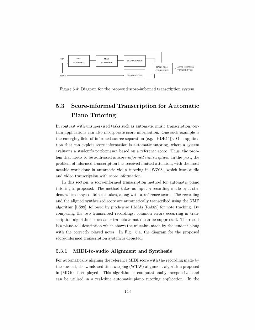
MIDI
AUDIO
MIDI
ALIGNMENT
MIDI
SYNTHESISTRANSCRIPTION
TRANSCRIPTION
PIANO-ROLL
COMPARISON
SCORE-INFORMED
TRANSCRIPTION
Figure 5.4: Diagram for the proposed score-informed transcription system.
5.3 Score-informed Transcription for Automatic
Piano Tutoring
In contrast with unsupervised tasks such as automatic music transcription, cer-
tain applications can also incorporate score information. One such example is
the emerging field of informed source separation (e.g. [HDB11]). One applica-
tion that can exploit score information is automatic tutoring, where a system
evaluates a student’s performance based on a reference score. Thus, the prob-
lem that needs to be addressed is score-informed transcription. In the past, the
problem of informed transcription has received limited attention, with the most
notable work done in automatic violin tutoring in [WZ08], which fuses audio
and video transcription with score information.
In this section, a score-informed transcription method for automatic piano
tutoring is proposed. The method takes as input a recording made by a stu-
dent which may contain mistakes, along with a reference score. The recording
and the aligned synthesized score are automatically transcribed using the NMF
algorithm [LS99], followed by pitch-wise HMMs [Rab89] for note tracking. By
comparing the two transcribed recordings, common errors occurring in tran-
scription algorithms such as extra octave notes can be suppressed. The result
is a piano-roll description which shows the mistakes made by the student along
with the correctly played notes. In Fig. 5.4, the diagram for the proposed
score-informed transcription system is depicted.
5.3.1 MIDI-to-audio Alignment and Synthesis
For automatically aligning the reference MIDI score with the recording made by
the student, the windowed time warping (WTW) alignment algorithm proposed
in [MD10] is employed. This algorithm is computationally inexpensive, and
can be utilised in a real-time automatic piano tutoring application. In the
143

experiments performed in [MD10], it was shown that the alignment algorithm
can correctly align 97% of the audio note onsets in the test set employed, using
a 2 sec tolerance (accuracy drops to 73.6% using a 100ms tolerance).
The result is an aligned MIDI file, which afterwards is synthesized using the
TiMidity synthesizer using the Merlin Vienna soundfont library5. For compar-
ative purposes, manually-aligned MIDI files are also produced and synthesized,
which are described in subsection 5.3.5.
5.3.2 Multi-pitch Detection
As in the harpsichord-specific transcription system of Section 5.2, for transcrib-
ing piano recordings we employ the NMF algorithm with β-divergence [Kom07],
using pre-extracted piano templates. As explained in the previous section, the
NMF algorithm with β-divergence is computationally inexpensive and it has
been shown to produce reliable results in piano-specific transcription [DCL10].
Firstly, spectral templates for the complete piano note range are extracted,
corresponding to notes from A0 to C8. We use recordings from 3 chromatic
scales from a Yamaha U3 Disklavier, which is also used for the test recordings. In
addition, we employ isolated note samples from 3 piano models from the MAPS
database [EBD10]. The fact that we are using training templates from the same
piano source as in the test set is a reasonable assumption given the specific
tutoring application, since the student can provide training examples in a setup
stage. If templates from the same source are not available, general-purpose
templates from e.g. the MAPS database can be used (related experiments shown
in subsection 5.3.5). For extracting the templates, the CQT [SK10] is employed
using a resolution of 120 bins/octave and lowest frequency 27.5 Hz. Next,
the NMF algorithm [LS99] as shown in eq. (2.6) using a single component is
employed for extracting the template from an isolated note recording.
For the multi-pitch detection step, the NMF model with β-divergence is
employed [Kom07] (details of the algorithm are given in subsection 2.3.3). For
the present experiments, we used β = 0.5, which was shown to produce the
best results for piano transcription in [DCL10]. Since in our case the spectral
template matrix is fixed, only the gain is iteratively updated (after random
initialization) using eq. (5.2). Convergence is observed at 10-15 iterations.
For piano transcription, the spectral template matrix W is created by con-
catenating the spectral templates from either the 3 sets of the Disklavier or the
5http://ocmnet.com/saxguru/Timidity.htm
144

MAPS templates:
W = [W(1) W(2) W(3)]. (5.5)
Thus, W ∈ RΩ×264, where Ω is the log-spectrum size. After the NMF update
rule of (5.2) is applied to the input log-spectrogram V ∈ RΩ×T (where T is the
frame length), the pitch activation matrix is created by adding the component
vectors from H that correspond to the same pitch:
H′p,t = Hp,t +Hp+88,t +Hp+176,t (5.6)
where H′ ∈ R88×T .
5.3.3 Note Tracking
As in the automatic transcription systems presented in Chapters 3 and 4, note
tracking is performed on the pitch activations of the original and synthesized
audio using on/off pitch-wise HMMs, using as input in the observation function
of (4.14) the pitch activation H′. For details on the note tracking procedure,
the reader is referred to subsection 4.2.4.
In order to set the value of parameter λ in (4.14) for the original recording, we
use one piece from the dataset for training (detailed in subsection 5.3.5). Also,
two additional piano-rolls from the transcribed recording using different values
for λ are extracted, thus creating a ‘strict’ transcription (with high precision
and low recall) and a ‘relaxed’ transcription (with high recall and low precision),
which will be utilised in the output of the proposed system. The values of λ
that are used for the normal, strict, and relaxed transcription, are respectively
1.3, 1.0, 2.1.
Finally, the resulting piano-rolls are processed in order to detect any repeated
notes which might appear in the final piano-roll as a continuous event (e.g.
trills). For the piano, detecting note onsets can be achieved by simply detecting
energy changes. Thus, peak detection is performed using the activation matrix
for each detected note. If a peak is detected at least 200ms after the onset, then
the note is split into two.
5.3.4 Piano-roll Comparison
In order to compare the performance of the student with the aligned score,
additional information is utilised using the transcribed synthesized score, as well
145

Algorithm 1 Piano-roll comparison for score-informed transcription
Input: prStudent, prSynth, prGT1: for each onset(p, t) ∈ prGT do
2: if onset(p, t) ∈ prStudent then3: prResult(p, t) = correct note4: else
5: if onset(p, t) ∈ prSynth then
6: prResult(p, t) = missed note7: else
8: prResult(p, t) = correct note9: end if
10: end if
11: end for
12: for each onset(p, t) ∈ prStudent do13: if onset(p, t) /∈ prGT ∪ prSynth then
14: prResult(p, t) = extra played note15: end if
16: end for
17: return prResult
as the strict and relaxed transcriptions of the recording. The motivation is that
automatic transcription algorithms typically contain false alarms (such as octave
errors) and missed detections (usually in the case of dense chords). However,
the transcribed synthesized score might also contain these errors. Thus, it can
assist in eliminating any errors caused by the transcription algorithm instead of
attributing them to the student’s performance.
Two assumptions are made in the algorithm: firstly, the recording does not
contain any structural errors. Thus, only local errors can be detected, such as
missed or extra notes played by the student. Secondly, evaluation is performed
by only examining note onsets, thus discarding note durations.
The process comparing the piano-roll for the transcribed recording (prStudent),
the synthesized MIDI (prSynth), and the aligned MIDI (prGT ) is given in Al-
gorithm 1. The tolerance for onset(p, t) is set to ±200ms. In line 8, when an
onset is present in the ground truth but is absent in both transcriptions, then
we do not have enough knowledge to determine the existence of that note and
it is set as correct.
After Algorithm 1 is completed, the extra and missed notes present in
prResult are re-processed using the ‘strict’ piano-roll prStrict and the ‘relaxed’
piano-roll prRelaxed, respectively. The notion is that if that same extra note
is not present in prStrict, then it is simply caused by a deficiency in the tran-
146
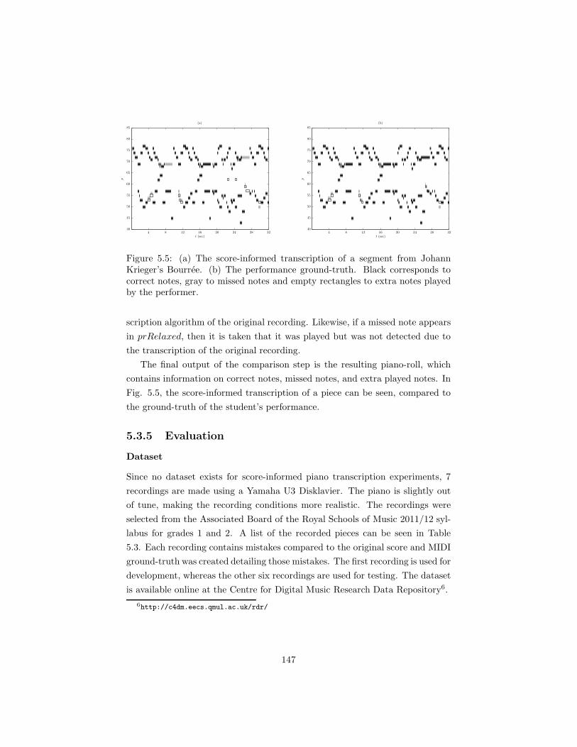
p
t (sec)
(b)p
t (sec)
(a)
4 8 12 16 20 24 28 324 8 12 16 20 24 28 3240
45
50
55
60
65
70
75
80
85
40
45
50
55
60
65
70
75
80
85
Figure 5.5: (a) The score-informed transcription of a segment from JohannKrieger’s Bourree. (b) The performance ground-truth. Black corresponds tocorrect notes, gray to missed notes and empty rectangles to extra notes playedby the performer.
scription algorithm of the original recording. Likewise, if a missed note appears
in prRelaxed, then it is taken that it was played but was not detected due to
the transcription of the original recording.
The final output of the comparison step is the resulting piano-roll, which
contains information on correct notes, missed notes, and extra played notes. In
Fig. 5.5, the score-informed transcription of a piece can be seen, compared to
the ground-truth of the student’s performance.
5.3.5 Evaluation
Dataset
Since no dataset exists for score-informed piano transcription experiments, 7
recordings are made using a Yamaha U3 Disklavier. The piano is slightly out
of tune, making the recording conditions more realistic. The recordings were
selected from the Associated Board of the Royal Schools of Music 2011/12 syl-
labus for grades 1 and 2. A list of the recorded pieces can be seen in Table
5.3. Each recording contains mistakes compared to the original score and MIDI
ground-truth was created detailing those mistakes. The first recording is used for
development, whereas the other six recordings are used for testing. The dataset
is available online at the Centre for Digital Music Research Data Repository6.
6http://c4dm.eecs.qmul.ac.uk/rdr/
147
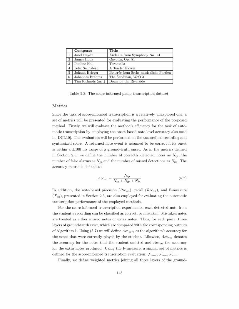
Composer Title
1 Josef Haydn Andante from Symphony No. 942 James Hook Gavotta, Op. 813 Pauline Hall Tarantella4 Felix Swinstead A Tender Flower5 Johann Krieger Bourree from Sechs musicalishe Partien6 Johannes Brahms The Sandman, WoO 317 Tim Richards (arr.) Down by the Riverside
Table 5.3: The score-informed piano transcription dataset.
Metrics
Since the task of score-informed transcription is a relatively unexplored one, a
set of metrics will be presented for evaluating the performance of the proposed
method. Firstly, we will evaluate the method’s efficiency for the task of auto-
matic transcription by employing the onset-based note-level accuracy also used
in [DCL10]. This evaluation will be performed on the transcribed recording and
synthesized score. A returned note event is assumed to be correct if its onset
is within a ±100 ms range of a ground-truth onset. As in the metrics defined
in Section 2.5, we define the number of correctly detected notes as Ntp , the
number of false alarms as Nfp and the number of missed detections as Nfn . The
accuracy metric is defined as:
Accon =Ntp
Ntp +Nfp +Nfn
(5.7)
In addition, the note-based precision (Preon), recall (Recon), and F-measure
(Fon), presented in Section 2.5, are also employed for evaluating the automatic
transcription performance of the employed methods.
For the score-informed transcription experiments, each detected note from
the student’s recording can be classified as correct, or mistaken. Mistaken notes
are treated as either missed notes or extra notes. Thus, for each piece, three
layers of ground-truth exist, which are compared with the corresponding outputs
of Algorithm 1. Using (5.7) we will define Acccorr as the algorithm’s accuracy for
the notes that were correctly played by the student. Likewise, Accmn denotes
the accuracy for the notes that the student omitted and Accen the accuracy
for the extra notes produced. Using the F-measure, a similar set of metrics is
defined for the score-informed transcription evaluation: Fcorr , Fmn , Fen .
Finally, we define weighted metrics joining all three layers of the ground-
148

Accon Fon Preon ReconRecording 83.88% 91.13% 93.34% 89.11%
Manual MIDI 84.73% 91.57% 93.56% 89.73%Automatic MIDI 89.77% 94.55% 95.05% 94.09%
Table 5.4: Automatic transcription results for score-informed transcriptiondataset.
truth. Given that Ncorr is the number of correctly played notes in the perfor-
mance of the student, Nmn is the number of notes missed and Nen is the number
of extra notes, the weighted accuracy is defined as:
Accw =NcorrAcccorr +NmnAccmn +NenAccen
Ncorr +Nmn +Nen
(5.8)
A similar definition can be made for a weighted F-measure, denoted as Fw.
Results
In Table 5.4, the automatic transcription results for the original recording and
the synthesized MIDI (using manual and automatic alignment) are shown. In all
cases the performance of the NMF-based transcription algorithm is quite high,
with the Fon always surpassing 90%. The performance difference between the
transcription of the manual and automatic MIDI is due to the fact that the note
velocities (dynamics) are preserved in the synthesized manually-aligned MIDI.
It should be stressed that when transcribing the synthesized MIDI, templates
from the MAPS database [EBD10] were used, whereas when transcribing the
original recording, templates from the Disklavier were utilised. When using the
MAPS templates for transcribing the recordings, Fon drops to 80.43%. When
simple thresholding on H′ is employed instead of the HMM-based note tracking
procedure, the average Fon for the recordings drops to 84.92%.
In Table 5.5, score-informed transcription results are presented, using either
manually-aligned or automatically-aligned MIDI. For the manually-aligned case,
it can be seen that the method reaches very high accuracy for the correctly
played notes by the student, while the detection performance for missed or
extra notes is lower. However, the overall performance of the method in terms
of Fw is quite high, reaching 96.76%. When automatically-aligned MIDI is used,
the system performance is diminished, which is expected, as additional errors
from imperfect alignment are introduced. The biggest decrease in performance
149

Fw Accw Acccorr Accmn AccenManual MIDI 96.76% 94.38% 97.40% 70.63% 75.27%
Automatic MIDI 92.93% 88.20% 93.17% 49.16% 60.49%
Table 5.5: Score-informed transcription results.
can be observed for the missed notes by the student. This can be attributed
to the fact that the alignment algorithm might place the non-played notes at
different positions compared to the ground-truth. Still, the overall performance
of the system using automatically-aligned MIDI files reaches an Fw of 92.93%.
In order to test the performance of different components of the proposed
method, comparative experiments are performed by disabling the process for de-
tecting repeated notes, using both manually-aligned and automatically-aligned
MIDI. Using the manually-aligned score, Fw = 92.79%while using the automatically-
aligned score, Fw = 89.04%. Another experiment is performed using the tem-
plates from the MAPS dataset [EBD10] for transcribing the recording. Using
the manually-aligned MIDI, Fw = 90.75% while using the automatically-aligned
MIDI, Fw = 85.94%. Without processing prResults with the ‘strict’ and
‘relaxed’ piano-rolls, the score-informed transcription results using manually-
aligned scores reach Fw = 94.92% and using automatically-aligned scores reach
Fw = 90.82%. A final comparative experiment is performed by utilizing only
the piano-roll of the aligned ground-truth for score information, instead of also
using the piano-roll of the transcribed synthesized score. In this case, using the
manually-aligned score Fw = 93.55% and using the automatically-aligned score
Fw = 89.47%, which demonstrates that transcribing the synthesized score can
assist in improving performance for a score-informed transcription system.
5.3.6 Discussion
This section proposed a system for score-informed transcription which is ap-
plied to automatic piano tutoring. Results indicate that using manually-aligned
scores, the proposed method can successfully analyze the student’s performance,
making it useful for real-life applications. Using automatically-aligned scores
produces somewhat lower performance especially when the student deviates
from the score.
Score-informed transcription is a relatively unexplored research field and
several of its sub-problems could be improved, for example creating robust
150

instrument-specific transcription algorithms. Future directions include the cre-
ation of a MIDI-to-audio alignment algorithm specifically tailored for the piano
alignment task, operating with higher precision as this was shown to be an
important factor in the proposed method’s performance. In addition, the detec-
tion of structural errors such as missed or replicated segments can be achieved
through a more sophisticated alignment algorithm.
5.4 Characterisation of Acoustic Scenes using
SI-PLCA
The temporally-constrained shift-invariant transcription model that was pro-
posed in Section 4.4 can also be utilised in other audio modelling applications.
In this section, the model of Section 4.4 is modified and applied to the field of
computational auditory scene analysis (CASA) [WE06], and more specifically
to the problem of acoustic scene characterization.
5.4.1 Background
The problem of modeling acoustic scenes is one of the most challenging tasks
in the CASA field [WE06]. It is closely related to the problem of detecting
and classifying acoustic events within a scene, and has numerous applications
in audio processing. In the literature the problem is also called context recogni-
tion [EPT+06]. In the case of scene categorisation or characterization, we are
interested in specifying the environment of the recording, which is informed by
the types of events that are present within the scene of interest. The problem
is especially challenging in the case of a real-world scenario with an unlimited
set of events which could also overlap in time.
Regarding related literature, Mesaros et al. [MHK11] proposed a system for
sound event detection which employed PLCA [SRS06] (also presented in sub-
section 2.3.3) for separating and detecting overlapping events. The system was
tested in a supervised scenario using a dataset of 103 recordings classified into
10 different scenes, containing events from 61 classes. In [CE11], Cotton and El-
lis utilised the NMD algorithm [Sma04a] (also presented in subsection 2.3.3) for
non-overlapping event detection. A comparison was made between NMD with a
frame-based approach using Mel-frequency cepstral coefficients (MFCCs). Ex-
periments performed on a dataset collected under the CHIL project, consisting
151
of 16 different event classes, showed that a combination of the NMD system and
the frame-based system yielded the best results.
In some cases, the salient events that characterise the scene are not known
a priori, or may be hard to learn from training data due to the large discrep-
ancy between two acoustic realizations of the same event. This leads to an
unsupervised formulation of the scene description problem, where we want the
algorithm to be able to extract in an unsupervised manner the events that de-
scribe the scene. Following this approach, Cauchi [Cau11] proposed a method
for classifying auditory scenes in an unsupervised manner using sparse NMF.
After extracting spectral basis vectors from acoustic scenes, each basis is con-
verted into MFCCs for compactness. A distance metric is defined for measuring
the difference between extracted dictionaries from different scenes. Evaluation
is performed on a corpus of 66 recordings taken from several train stations
[TSP+08], originally created for a perceptual study on acoustic scene categori-
sation, resulting in six acoustic scene classes. Experiments made by comparing
the sparse NMF with a bag-of-features approach from [ADP07] showed that the
NMF algorithm is able to successfully extract salient events within an acoustic
scene.
5.4.2 Proposed Method
In this section, we build upon the work by Cauchi [Cau11] and propose a method
for modeling and classifying acoustic scenes in an unsupervised manner using a
temporally-constrained shift-invariant model. This level of temporality will con-
trol the appearance of the time-frequency patches in a recording and can be sup-
ported by using the proposed HMM-constrained SI-PLCA model presented in
Section 4.4, also modified for supporting time-frequency patches instead of one-
dimensional spectra. In the model, the component activation function would
consist of zeros in case of inactivity and ones at the time instants where an
event would appear. Each HMM in the model can represent a certain compo-
nent, which would be represented using a two-state, on/off model. This on/off
model would serve as an event indicator function, which would enforce temporal
constraints in the auditory scene activation matrix. Fig. 5.6 shows the diagram
for the proposed system.
152
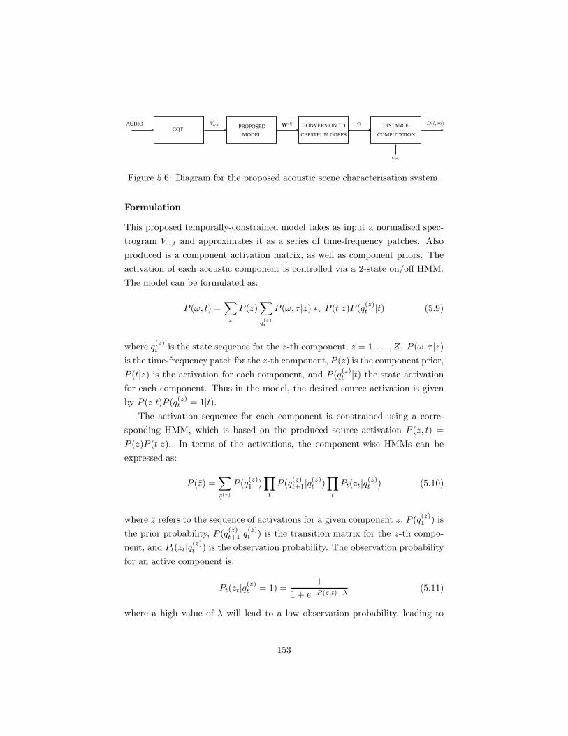
CQT PROPOSED
MODEL
CONVERSION TO
CEPSTRUM COEFS
AUDIO DISTANCE
COMPUTATION
W(l) clVω,t
cm
D(l,m)
Figure 5.6: Diagram for the proposed acoustic scene characterisation system.
Formulation
This proposed temporally-constrained model takes as input a normalised spec-
trogram Vω,t and approximates it as a series of time-frequency patches. Also
produced is a component activation matrix, as well as component priors. The
activation of each acoustic component is controlled via a 2-state on/off HMM.
The model can be formulated as:
P (ω, t) =∑
z
P (z)∑
q(z)t
P (ω, τ |z) ∗τ P (t|z)P (q(z)t |t) (5.9)
where q(z)t is the state sequence for the z-th component, z = 1, . . . , Z. P (ω, τ |z)
is the time-frequency patch for the z-th component, P (z) is the component prior,
P (t|z) is the activation for each component, and P (q(z)t |t) the state activation
for each component. Thus in the model, the desired source activation is given
by P (z|t)P (q(z)t = 1|t).
The activation sequence for each component is constrained using a corre-
sponding HMM, which is based on the produced source activation P (z, t) =
P (z)P (t|z). In terms of the activations, the component-wise HMMs can be
expressed as:
P (z) =∑
q(z)
P (q(z)1 )
∏
t
P (q(z)t+1|q
(z)t )
∏
t
Pt(zt|q(z)t ) (5.10)
where z refers to the sequence of activations for a given component z, P (q(z)1 ) is
the prior probability, P (q(z)t+1|q
(z)t ) is the transition matrix for the z-th compo-
nent, and Pt(zt|q(z)t ) is the observation probability. The observation probability
for an active component is:
Pt(zt|q(z)t = 1) =
1
1 + e−P (z,t)−λ(5.11)
where a high value of λ will lead to a low observation probability, leading to
153
an ‘off’ state. The formulation of the observation function is similar to the one
used for note tracking in subsection 4.2.4.
Parameter Estimation
As in the model of Section 4.4, the unknown parameters in the model can
be estimated using the EM algorithm [DLR77]. For the Expectation step, we
compute the posterior for all the hidden variables:
P (z, τ, q(1)t , . . . , q
(Z)t |z, ω, t) = P (q
(1)t , . . . , q
(Z)t |z)P (z, τ |q
(1)t , . . . , q
(Z)t , ω, t)
(5.12)
Since we are utilising independent HMMs, the joint probability for all hidden
source states is given by:
Pt(q(1)t , . . . , q
(Z)t |z) =
Z∏
z=1
Pt(q(z)t |z) (5.13)
where
Pt(q(z)t |z) =
Pt(z, q(z)t )
∑q(z)t
Pt(z, q(z)t )
=αt(q
(z)t )βt(q
(z)t )
∑q(z)t
αt(q(z)t )βt(q
(z)t )
(5.14)
and αt(q(z)t ), βt(q
(z)t ) are the forward and backward variables for the z-th HMM
[Rab89], which are computed recursively using (4.22)-(4.23).
The second term of (5.12) can be computed using Bayes’ theorem:
P (z, τ |q(1)t , . . . , q
(Z)t , ω, t) = P (z, τ |ω, t) =
P (z)P (ω, τ |z)P (t− τ |z)∑z
∑τ P (z)P (ω, τ |z)P (t− τ |z)|t)
(5.15)
Finally, the posterior for the component transition matrix is given by:
Pt(qt, qt+1|z) =αt(qt)P (qt+1|qt)βt+1(qt+1)Pt(zt+1|qt+1)∑
qt,qt+1αt(qt)P (qt+1|qt)βt+1(qt+1)Pt(zt+1|qt+1)
(5.16)
For the Maximization step, the update rules for estimating the unknown
parameters are:
P (z) =
∑ω,τ,t
∑q(z)t
Vω,tP (z, τ, q(1)t , . . . , q
(Z)t |ω, t)
∑z,ω,τ,t
∑q(z)t
Vω,tP (z, τ, q(1)t , . . . , q
(Z)t |ω, t)
(5.17)
154
P (ω, τ |z) =
∑t
∑q(z)t
Vω,tP (z, τ, q(1)t , . . . , q
(Z)t |ω, t)
∑ω,τ,t
∑q(z)t
Vω,tP (z, τ, q(1)t , . . . , q
(Z)t |ω, t)
(5.18)
P (t|z) =
∑ω,τ
∑q(z)t
Vω,t+τP (z, τ, q(1)t , . . . , q
(Z)t |ω, t+ τ)
∑t,ω,τ
∑q(z)t
Vω,t+τP (z, τ, q(1)t , . . . , q
(Z)t |ω, t+ τ)
(5.19)
P (q(z)t+1|q
(z)t ) =
∑t P (q
(z)t , q
(z)t+1|z)∑
q(z)t+1
∑t P (q
(z)t , q
(z)t+1|z)
(5.20)
P (q(z)1 ) = P1(q
(z)1 |z) (5.21)
where∑
q(z)t
=∑q(1)t
· · ·∑
q(Z)t
. Eq. (5.21) updates the component prior using
the posterior of eq. (5.14). The final event activation is given by the activation
for each component given by the model and the probability for an active state
for the corresponding component:
P (z, t, q(z)t = 1) = P (z)P (t|z)P (q
(z)t = 1|t) (5.22)
As in the model of Section 4.4, sparsity constraints are applied to P (t|z) using
the entropic prior of [Bra99] applied in the PLCA context in [Sma09] in order
to obtain a sparse component activation. For all the experiments performed in
this paper, the length of each basis has been set to 400ms.
Acoustic Scene Distance
For computing the distance between acoustic scenes, we first compute the CQT
[SK10] of each 44.1 kHz recording with a log-frequency resolution of 5 bins per
octave and an 8-octave span with 27.5 Hz set as the lowest frequency. The step
size is set to 40 ms. Afterwards, time-frequency patches are extracted using the
proposed HMM-constrained SIPLCA algorithm with Z ∈ 10, 25, 50 bases and
λ = 0.005 (the value was set after experimentation). Sparsity was enforced to
P (t|z) with sparsity parameter values sH ∈ 0, 0.1, 0.2, 0.5. In all cases the
length of each basis is set to 400 ms.
For each basis Wz = P (ω, τ |z), very small values (< 0.001) are replaced
by the median value of Wz. Afterwards, a vector of 13 cepstral coefficients
is computed for each basis frame w[k] = Wz[k, t], k = 1, . . . ,K, in order to
result in a compact representation for computational speed purposes. In order to
convert a vector w[k] into cepstral coefficients, we employ the formula presented
155

in [Bro99]:
ci =
K∑
k=1
log(w[k]) cos
(i
(k −
1
2
)π
K
)(5.23)
where i = 1, . . . , 13. Each vector of cepstral coefficients is then normalised to
the [0,1] region. The first coefficient, which corresponds to the DC component
of the signal, is dropped. Finally, for each time-frequency basis, the coefficients
are summed together over time, thus resulting in a single vector representing
a basis. This compressed basis vector is denoted as wz, where z denotes the
component index.
For computing the distance between a scene l and a scene m, we employ
the same steps as in [Cau11]. Firstly, we compute the elementwise distance
between a basis w(l)z , z = 1, . . . , Z and the nearest basis of dictionary W(m)
(which includes all vectors w(m)z ):
dz(l,m) = minj∈[1,Z]
||w(l)z −w
(m)j || (5.24)
The final distance between two acoustic scenes is defined as:
D(l,m) =
Z∑
z=1
dz(l,m) + dz(m, l) (5.25)
Equation (5.25) is formulated in order for the distance measure between two
scenes to be symmetric. In the end, the acoustic scene distance matrix D is
used for evaluation.
It should be noted that quantifying the distance between two basis vectors
by considering the Euclidean distance of their time average most probably leads
to a loss of descriptive power of our model. This choice is made for tractability
purposes. Indeed, for the corpus used in this study and 50 bases per item,
building the matrix D involves making about 1012 comparisons. Finding an
efficient way of considering the time axis during the distance computation is left
for future research.
5.4.3 Evaluation
Dataset
For the acoustic scene classification experiments we employ the dataset created
by J. Tardieu [TSP+08]. The dataset was originally created for a perceptual
156
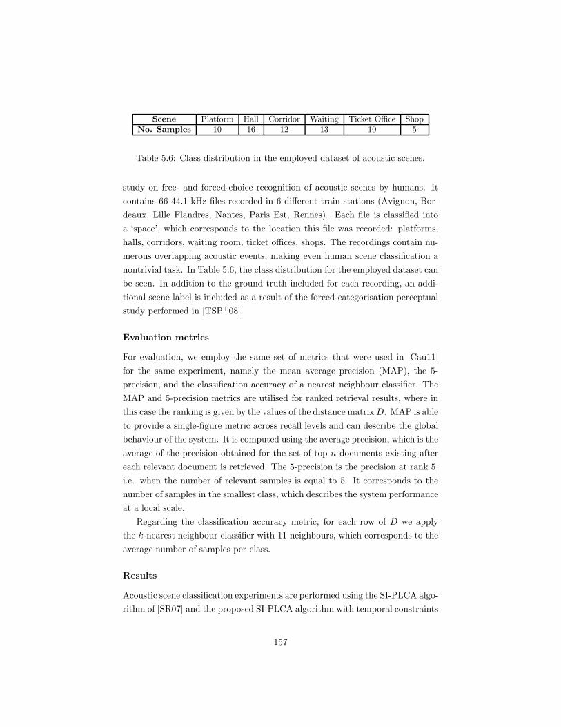
Scene Platform Hall Corridor Waiting Ticket Office ShopNo. Samples 10 16 12 13 10 5
Table 5.6: Class distribution in the employed dataset of acoustic scenes.
study on free- and forced-choice recognition of acoustic scenes by humans. It
contains 66 44.1 kHz files recorded in 6 different train stations (Avignon, Bor-
deaux, Lille Flandres, Nantes, Paris Est, Rennes). Each file is classified into
a ‘space’, which corresponds to the location this file was recorded: platforms,
halls, corridors, waiting room, ticket offices, shops. The recordings contain nu-
merous overlapping acoustic events, making even human scene classification a
nontrivial task. In Table 5.6, the class distribution for the employed dataset can
be seen. In addition to the ground truth included for each recording, an addi-
tional scene label is included as a result of the forced-categorisation perceptual
study performed in [TSP+08].
Evaluation metrics
For evaluation, we employ the same set of metrics that were used in [Cau11]
for the same experiment, namely the mean average precision (MAP), the 5-
precision, and the classification accuracy of a nearest neighbour classifier. The
MAP and 5-precision metrics are utilised for ranked retrieval results, where in
this case the ranking is given by the values of the distance matrixD. MAP is able
to provide a single-figure metric across recall levels and can describe the global
behaviour of the system. It is computed using the average precision, which is the
average of the precision obtained for the set of top n documents existing after
each relevant document is retrieved. The 5-precision is the precision at rank 5,
i.e. when the number of relevant samples is equal to 5. It corresponds to the
number of samples in the smallest class, which describes the system performance
at a local scale.
Regarding the classification accuracy metric, for each row of D we apply
the k-nearest neighbour classifier with 11 neighbours, which corresponds to the
average number of samples per class.
Results
Acoustic scene classification experiments are performed using the SI-PLCA algo-
rithm of [SR07] and the proposed SI-PLCA algorithm with temporal constraints
157

Z = 50
Z = 25
Z = 10
(a)
sH
MAP
0 0.1 0.2 0.50.26
0.27
0.28
0.29
0.3
0.31
0.32
0.33
0.34
0.35
Z = 50
Z = 25
Z = 10
(b)
sH
MAP
0 0.1 0.2 0.50.26
0.27
0.28
0.29
0.3
0.31
0.32
0.33
0.34
0.35
Figure 5.7: Acoustic scene classification results (MAP) using (a) the SI-PLCAalgorithm (b) the TCSI-PLCA algorithm, with different sparsity parameter(sH) and dictionary size (Z).
(named TCSI-PLCA for brevity). Comparative results are also reported using
a bag-of-frames (BOF) approach of [ADP07] reported in [Cau11]. The bag-of-
frames method computes several audio features which are fed to a Gaussian
mixture model classifier. The NMF method of [Cau11] is also implemented and
tested. Results are also compared with the human perception experiment re-
ported in [TSP+08]. Experiments are performed using different dictionary sizes
Z and sparsity parameters sH (details on the range of values can be seen in the
previous subsection).
The best results using each employed classifier are presented in Table 5.7.
The proposed temporally-constrained SIPLCAmodel outperforms all other clas-
158

Model MAP 5-Precision
Human Perception [TSP+08] 0.62 0.73
Random 0.25 0.18BOF [ADP07] 0.24 0.18
NMF (Z = 50, sH = 0.99) 0.32 0.29SI-PLCA (Z = 25, sH = 0.2) 0.33 0.35TCSI-PLCA (Z = 25, sH = 0.2) 0.34 0.36
Table 5.7: Best MAP and 5-precision results for each model.
sifiers using both metrics, apart from the human forced categorisation experi-
ment. The proposed method slightly outperforms the standard SI-PLCA algo-
rithm, which in turn outperforms the NMF algorithm. It can also be seen that
the BOF method is clearly not suitable for such an experiment, since the au-
dio features employed in this method are more appropriate for non-overlapping
events, whereas the dataset that is utilised contains concurrent events and a
significant level of background noise. However, the human categorisation exper-
iment from [TSP+08] outperforms all other approaches.
More detailed results for the SI-PLCA algorithm using different sparsity
parameter values and different numbers of extracted bases (Z) can be seen in
Fig. 5.7 (a). In all cases, enforcing sparsity improves performance. It can
also be seen that the best performance is reported for Z = 25, although the
performance of the system using Z = 50 improves when greater sparsity on
P (t|z) is encouraged. Detailed results for the proposed TCSI-PLCA method
can be seen in Fig. 5.7 (b), using different dictionary sizes and sparsity values.
It can be seen that the performance reaches a peak when sH = 0.2, for the case
of Z = 25. When using a dictionary size of Z = 50, the performance of the
proposed method is slightly decreased. Thus, selecting the appropriate number
of components is important in the performance of the proposed method, since
using too many components will lead to a parts-based representation which in
the unsupervised case will lead to non representative dictionaries. Likewise,
selecting too few bases will lead to a less descriptive model of the input signal.
Regarding classification accuracy using 11-nearest neighbours, results are
shown in Table 5.8. Again, the TCSI-PLCA method outperforms all the other
automatic approaches. In this case however, the non-negative matrix factoriza-
tion approach from [Cau11] outperforms the SIPLCA algorithm by 0.5%. For
the TCSI-PLCA algorithm, the best performance is again reported for sH = 0.2,
159

Classifier Accuracy %
Human Perception [TSP+08] 54.8%
Random 16.6%BOF [ADP07] 19.7%
NMF (Z = 50, sH = 0) 34.1%SI-PLCA (Z = 25, sH = 0.5) 33.6%TCSI-PLCA (Z = 50, sH = 0.2) 35.0%
Table 5.8: Best classification accuracy for each model.
while for the NMF approach the best performance is reported for sH = 0. Re-
garding dictionary size, the best results are reported for Z = 50.
Comparative experiments are performed by selecting only basis vectors that
correspond to a sparse activation P (t|z). In the PLCA domain, the sparseness
criterion can be given by maximizing the l2 norm as in [Sma11], due to the fact
that all elements of the activation matrix take values between 0 and 1. However,
the performance of the SI-PLCA and TCSI-PLCA algorithms in fact decreased
slightly when selecting only the basis vectors that corresponded to the sparsest
activations. This issue may be addressed in the future by enforcing sparsity
only to certain components that represent salient events and keeping the rest of
the components (which could represent noise) without enforcing sparsity.
5.4.4 Discussion
In this section we proposed a method for modeling and classifying acoustic scenes
using a temporally-constrained shift-invariant model similar to the one proposed
for automatic music transcription purposes in Section 4.4. In the classification
stage, each extracted time-frequency basis is converted into a compact vector of
cepstral coefficients for computational speed purposes. The employed dataset
consisted of recordings taken from six types of scenes at different train stations.
Comparative experiments were performed using a standard non-negative matrix
factorization approach, as well as a bag-of-frames algorithm which is based on
computing audio features. Results show that using shift-invariant models for
learning time-frequency patches improves classification performance. Moreover,
incorporating temporal constraints in the SI-PLCA model as well as enforcing
sparsity constraints in the component activation result in improved classification
performance.
160
However, the classification performance of the proposed computational meth-
ods is still significantly lower than the human forced categorisation task pre-
sented in [TSP+08]. We acknowledge that this performance is in our case an
upper bound that may not even be reached by purely data-driven methods since
humans most probably make extensive use of prior knowledge but the significant
gap between the human and computational performances indicates that there
is potentially room for improvement on the computational side.
In order to improve spectrogram factorization techniques such as NMF and
SI-PLCA, additional constraints and knowledge need to be incorporated into
the models. A hierarchical model which would consist of event classes and
component subclasses would result in a richer model, but would also require
prior information on the shape of each event in order to result in meaningful
time-frequency patches. Prior information can be provided by utilising training
samples of non-overlapping acoustic events. Also, an additional sparseness con-
straint could be imposed on the activation matrix, in order to control the number
of overlapping components present in the signal (instead of enforcing sparsity as
in the present work). In addition, instead of using a first-order Markov model
for imposing temporal constraints, a more complex algorithm which would be
able to model the duration of each event, such as a semi-Markov model [Yu10]
could be employed. Finally, finding an efficient way of comparing extracted
time frequency patches is also important. In this respect, we believe that lower
bounding approaches to the dynamic time warping technique are of interest
[Keo02, RCM+12].
5.5 Discussion
This chapter presented applications of proposed automatic music transcription
systems. The first two systems were applications of AMT to computational mu-
sicology, namely for modulation detection and temperament estimation. For the
system presented in Section 5.3, an algorithm for score-informed transcription
was proposed, which was applied to the problem of automatic piano tutoring.
Finally, in Section 5.4, the temporally-constrained shift-invariant model that
was proposed for automatic music transcription in Section 4.4 was applied to
the field of computational auditory scene analysis, namely for acoustic scene
characterisation.
The applications of automatic music transcription presented in this chapter
161

are but a small subset of the potential applications of AMT to music technology.
The creation of a robust AMT system can help in solving several problems in
the field of music information retrieval (MIR), such as music genre classification,
music similarity, cover song identification, and artist identification. It can also
improve the performance of problems which are based on low-level descriptors,
such as instrument identification and chord estimation. AMT can also bridge the
gap in systematic and computational musicology between current symbolic mu-
sic processing approaches and the use of audio recordings for addressing related
problems. Interactive systems for automatic improvisation and accompaniment
as well as for automatic tutoring can also benefit from automatic transcription
methods. Finally, the techniques developed for automatic transcription such
as the ones presented in Chapter 4 can also be used for other problems which
require the analysis and decomposition of time series data, such as the case of
acoustic scene characterisation that was presented in this chapter.
162
Chapter 6
Conclusions and Future
Perspectives
In this thesis, several methods for automatic music transcription have been pro-
posed using audio feature-based techniques and spectrogram factorization-based
techniques, in an attempt to exploit characteristics of the temporal evolution
of sounds. In addition, several applications of automatic transcription systems
were proposed, demonstrating the impact of AMT research in music technol-
ogy and audio processing. The majority of the work presented in this thesis
has been presented in international peer-reviewed journals and conferences, as
shown in Section 1.4. In this chapter, the main contributions of the thesis are
summarised and directions for future work are presented.
6.1 Summary
6.1.1 Audio feature-based AMT
In Chapter 3, methods for audio feature-based automatic music transcription
were proposed and evaluated. Initial work consisted of a system for multiple-F0
estimation of isolated piano sounds, which used pitch candidate selection and
rule-based refinement steps (Section 3.2). Contributions of that system were
a pitch salience function in the log-frequency domain which supported inhar-
monicity and tuning changes; a feature measuring spectral irregularity which
is robust to overlapping partials; and a feature based on the common ampli-
163

tude modulation assumption for eliminating octave errors. Experimental results
showed that the proposed system outperforms several state-of-the-art systems
for the task of multiple-F0 estimation of isolated piano sounds. A variant of the
proposed system for supporting complete recordings instead of isolated sounds
was publicly evaluated in the MIREX 2010 multiple-F0 estimation task [MIR].
Afterwards, a joint multiple-F0 estimation system was proposed for AMT,
followed by note tracking (Section 3.3). Contributions of that work were a noise
suppression algorithm based on a pink noise assumption; an overlapping partial
treatment procedure using the harmonic envelopes of pitch candidates; a pitch
set score function which incorporated several spectral and temporal features; an
algorithm for spectral envelope estimation in the log-frequency domain; and a
note tracking procedure using conditional random fields [LMP01]. The system
was evaluated using several datasets commonly used in AMT literature, where it
was shown that the proposed system outperforms several state-of-the-art AMT
systems for the same experiments. It was also shown that the joint multiple-F0
estimation algorithm of Section 3.3 performs better than the iterative multiple-
F0 estimation algorithm of Section 3.2, at the expense of increased computa-
tional cost. In addition, it was shown that the note tracking procedures using
hidden Markov models [Rab89] and conditional random fields [LMP01] helped
improve transcription performance compared to simple thresholding.
Finally, an extension of the joint multiple-F0 estimation system was pro-
posed, by explicitly incorporating information about note onsets and offsets
(Section 3.4). Contributions of this work include a note onset detection proce-
dure which incorporates tuning and pitch information from the pitch salience
function and a note offset detection procedure using pitch-wise hidden Markov
models [Rab89]. This system was evaluated using the same datasets as the
system of Section 3.3, and results demonstrate an improved transcription per-
formance using note-based metrics (instead of frame-based metrics), since this
system explicitly models note events. Also, in cases where hard onsets are
present, is was shown that explicitly incorporating note onset information im-
proves transcription performance.
6.1.2 Spectrogram factorization-based AMT
In Chapter 4, methods for automatic music transcription using spectrogram
factorization techniques were proposed and evaluated. Proposed systems ex-
tended the shift-invariant probabilistic latent component analysis (SI-PLCA)
164
model [SRS08b], for supporting multiple templates per pitch and instrument,
as well as for introducing temporal constraints for sound evolution, while at
the same time being able to model frequency modulations as shifts in the log-
frequency domain. Additionally, the proposed spectrogram factorization models
can be modified easily for instrument-specific transcription by changing instru-
ment templates.
The first proposed system consisted of a model based on SI-PLCA which
supported the use of multiple spectral templates per pitch, as well as per mu-
sical instrument (Section 4.2). The contribution of each source is time- and
pitch-dependent, making the model also suitable for instrument identification
in polyphonic music. Finally, the high-resolution time-pitch representation that
is the output of the system can also be used for pitch visualization purposes. The
system was evaluated using the same set of recordings as in Chapter 3, where
it was shown that the proposed model outperformed the audio feature-based
approaches in most cases. It was shown that a convolutive model can help im-
prove transcription accuracy compared to a non-convolutive linear model (e.g.
using PLCA [SRS06] or NMF [LS99]). Also, incorporating sparsity constraints
in the pitch and source activations improved transcription performance. The
system of Section 4.2 was also publicly evaluated in the MIREX 2011 contest,
where it ranked 2nd in the multiple-instrument note tracking task [MIR].
In Section 4.3, temporal constraints were incorporated within a single-source
SI-PLCA model using hidden Markov models [Rab89] for modelling the tempo-
ral evolution of notes. The proposed model expressed the evolution of mono-
phonic music sounds as a sequence of sound state templates, shifted across log-
frequency. Experimental results on pitch detection showed that the temporally-
constrained shift-invariant model outperformed a non-temporally-constrained
model for the same experiment, indicating that incorporating temporal con-
straints in multiple-instrument multi-pitch detection can further improve tran-
scription performance.
Finally, the temporal constraints of Section 4.3 were combined with the
multiple-instrument multi-pitch model of Section 4.2 in the proposed model of
Section 4.4. Thus, the contribution of this section was a system for multi-pitch
detection and multiple instrument assignment, supporting also multiple sets
of sound state templates per source. At the same time, the model supported
tuning changes and frequency modulations due to its shift-invariant nature.
Experiments showed that the proposed model outperforms the non-temporally
constrained model of Section 4.2, both for automatic transcription and instru-
165
ment assignment, and also outperforms state-of-the-art transcription systems in
the literature for the same experiments.
6.1.3 Transcription Applications
In Chapter 5 applications of the proposed AMT systems were presented, in order
to demonstrate the potential impact of automatic music transcription research
in music technology and audio processing.
In Section 5.1, the AMT system of Section 3.4 was utilised as front-end
for an automatic modulation detection system for J.S. Bach chorales. To the
author’s knowledge, this is the first study which utilised AMT for systematic
musicology research. Results comparing an audio input and a symbolic input
showed that although there are many differences between the transcribed audio
and the original score, the performance of the two systems for key detection is
similar, showing that AMT can be used as an audio front-end for certain tasks
in the systematic musicology field.
A computationally efficient harpsichord-specific transcription system was
proposed in Section 5.2 as a front-end for estimating temperament in harpsi-
chord recordings. The system was used to transcribe over 500 complete harpsi-
chord recordings taken from 22 CDs. The measured temperaments are compared
with the annotations found in CD sleeve notes and it was found that while this
information is mostly correct, there were several cases where a discrepancy in
temperament was found, raising an interesting issue about the nature of “ground
truth”.
A method for score-informed transcription was proposed in Section 5.3 and
was applied to automatic piano tutoring, in an effort to detect mistakes made by
piano students. It should be noted that the problem of score-informed transcrip-
tion is relatively unexplored, and a contribution of this work is the transcription
of the synthesized score along with the original recording. A score-informed pi-
ano transcription dataset was created by the author and is available online.
Results indicated that using manually-aligned scores, the proposed method can
successfully analyze the student’s performance. Also, it was shown that tran-
scribing the synthesized score helped improve score-informed transcription per-
formance.
Finally, in Section 5.4, the temporally-constrained shift-invariant transcrip-
tion model of Section 4.4 was modified for the problem of acoustic scene charac-
terisation in an unsupervised manner. Experimental results using train station
166
recordings showed that the proposed model outperforms NMF-based models
and that temporal constraints help improve classification accuracy. It was also
shown that the proposed transcription models can be used in non-music audio
processing applications.
6.2 Future Perspectives
Although the proposed systems outperform state-of-the-art systems, the overall
transcription performance is still considerably below that of a human expert,
and will most likely continue to be for some years, as the transcription problem
is inherently complex and the field has only recently started to grow.
As shown in this work, signal processing-based systems are computationally
inexpensive and have demonstrated encouraging transcription results, but have
problems with respect to generalisation (e.g. to different instrument sources).
Thus, signal processing-based systems cannot straightforwardly be used as a
basis for a more general system for analysing music signals, which could ad-
ditionally address the problems of instrument identification, source separation,
extraction of rhythmic information, etc. On the other hand, spectrogram fac-
torisation models produced competitive results, offering at the same time a
transparent model of operation which helps in extending these models for the
creation of more complex systems for music signal analysis. The main drawback
of spectrogram factorisation models is that they are computationally expensive.
It was also shown that AMT systems can effectively be used in other music
technology applications. Current tasks in music information retrieval (MIR)
such as genre classification, music similarity, and chord detection typically em-
ploy low-level features instead of utilising information from the transcribed
score. Although transcription-based techniques for MIR will most likely be
more computationally demanding compared to low-level feature-based tech-
niques, they can also offer a more complete framework for analysing music sig-
nals. This framework can be used as a basis for addressing many tasks (instead
of proposing task-specific MIR techniques) and can also be used for the extrac-
tion of high-level musicological features for music analysis. Another field where
AMT systems can be used is computational musicology; current applications
use symbolic data as input, whereas using an AMT system, research could be
performed from an audio front-end.
Proposed systems can be used as a basis for creating improved transcription
167

systems as well as systems for music signal analysis. In the process of carrying
out research and writing for the thesis, many ideas for future research emerged
regarding automatic transcription, note tracking, and instrument identification,
which will be detailed below.
Regarding improving transcription performance, the temporally-constrained
model of Section 4.4 can be modified to support whole-note templates instead of
a series of spectra for each sound state, resulting in a more constrained model,
albeit more demanding computationally. Since the duration of each note event
is arbitrary, each whole-note template can be scaled over time using dynamic
time warping techniques (e.g. [MD10]).
Different time-frequency representations can also be used as input to the
proposed AMT systems, in an effort to further improve transcription perfor-
mance. For example, the auditory models by Yang et al. [YWS92] can be used
instead of the constant-Q transform. Also, the use of spectral reassignment
was shown to outperform the short-time Fourier transform for automatic tran-
scription in [Hai03] and could be tested using the proposed systems. Another
avenue of research would be the use of several time-frequency representations,
using e.g. different window sizes. This would result in a tensorial input, which
could be transcribed by modifying currently proposed techniques for SI-PLCA
to probabilistic latent tensor factorization (PLTF) [CSS11].
Another way of improving transcription performance would be fusing differ-
ent AMT systems at the decision level (late fusion). In [HS10], it was shown
that combining several conservative onset detectors (with high precision and
low recall), an improvement can be achieved in onset detection; the same idea
can be utilised in the context of automatic transcription.
Computational efficiency is another issue, especially in the convolutive tran-
scription models of Chapter 4, which employ the EM algorithm. One way of
addressing this issue would be to keep the same model formulation but to utilise
a different algorithm for parameter estimation, which would be more computa-
tionally efficient, e.g. convolutive sparse coding [Vir04].
For further improving the SI-PLCA-based models of Chapter 4, in [DCL10]
it was shown that the NMF algorithm with β-divergence performed better than
the standard NMF algorithm. Since in [SRS08a] it was shown that the NMF
algorithm using the KL divergence is equivalent to the PLCA algorithm, in-
troducing β-divergences in the PLCA and SI-PLCA models could also further
improve transcription performance.
Regarding note tracking, all proposed transcription systems in Chapters 3
168

and 4 performed multiple-F0 estimation and note tracking separately. Tran-
scription performance could potentially improve by proposing a joint model
for multiple-F0 estimation and note tracking (similar to the one in [KNS07]),
which however would be less computationally efficient. One other way to im-
prove transcription performance with respect to the note tracking process would
be to utilise a key induction procedure which would assist in assigning priors
and transition probabilities using training data in the same key (instead of hav-
ing one transition matrix for all keys). Also, the present 2-state on/off models
for note tracking could be further extended by incorporating a musicological
model of note transitions at one level and chord transitions at a higher level, as
in [ROS09b].
Current note tracking models however do not explicitly model note dura-
tions, but only express note or chord transitions. Instead of using a first-order
Markov model for imposing temporal constraints, a more complex algorithm
which would be able to model the duration of each event, such as a semi-Markov
model [Yu10] can be employed. Such a development would also be of interest
for the acoustic scene characterisation experiments of Section 5.4, for modelling
the duration of specific events.
Finally, regarding instrument assignment, although the proposed model of
Section 4.4 outperformed other approaches for the same experiment, instrument
identification performance is still poor. However, the proposed spectrogram
factorization-based models could potentially improve upon instrument assign-
ment performance by utilizing the information provided by the source contri-
bution matrix Pt(s|p), combined with features for characterizing music timbre
(e.g. [Pee04]). Also, in the model of Section 4.4, the number of sound states
can also be made instrument-dependent by performing slight modifications to
the model, thus providing a more realistic model for each instrument.
169

Appendix A
Expected Value of Noise
Log-Amplitudes
We present the derivation for the expected value of noise log-amplitudes, which
is used in the proposed noise suppression algorithm for the joint multi-pitch
detection system of Section 3.3. We assume that the noise amplitude follows
an exponential distribution. In order to find the expected value of the noise
log amplitudes Elog(|Nc(ω)|), we adopt a technique similar to [Yeh08]. Let
Θ = log(Nc(ω)) = Φ(N):
EΘ =
∫ +∞
−∞
θP (θ)dθ =
∫ +∞
−∞
θP (Φ−1(θ))
∣∣∣∣dΦ−1(θ)
dθ
∣∣∣∣
=
∫ +∞
−∞
χθe−χeθ
eθdθ =
∫ +∞
0
χ log(ψ)e−χψdψ
= −γ − χ log(χ) ·
∫ +∞
0
e−χψdψ
= log(χ−1)− γ (A.1)
where γ is the Euler constant:
γ = −
∫ +∞
0
e−ψ log(ψ)dψ ≈ 0.57721. (A.2)
170
Appendix B
Log-frequency spectral
envelope estimation
An algorithm for posterior-warped log-frequency regularized spectral envelope
estimation is proposed, which is used in the joint multi-pitch detection sys-
tem of Section 3.3. Given a set of harmonic partial sequences (HPS) in the
log-frequency domain, the algorithm estimates the log-frequency envelope using
linear regularized discrete cepstrum estimation. In [DR03] a method for estimat-
ing the spectral envelope using discrete cepstrum coefficients in the Mel-scale
was proposed. The superiority of discrete cepstrum over continuous cepstrum
coefficients and linear prediction coefficients for spectral envelope estimation
was argued in [SR99]. Other methods for envelope estimation in the linear
frequency domain include a weighted maximum likelihood spectral envelope es-
timation technique in [BD08], which was employed for multiple-F0 estimation
experiments in [EBD10]. The proposed algorithm can be outlined as follows:
1. Extract the harmonic partial sequence HPS [p, h] and corresponding log-
frequency bins ωp,h for a given pitch p and harmonic index h = 1, . . . , 13.
2. Convert the log-frequency bins ωp,h to linear angular frequencies ωp,h
(where the sampling rate is fs = 44.1 kHz and the lowest frequency for
analysis is flow = 27.5 Hz):
ωp,h = 27.5 ·2π
fs· 2
ωp,h120 (B.1)
171
3. Perform spectral envelope estimation on HPS [p, h] and ωp,h using the
linear regularized discrete cepstrum. Coefficients cp are estimated as:
cp = (MTpMp + ρK)−1MT
p ap (B.2)
where ap = [ln(HPS [p, 1]), . . . , ln(HPS [p,H ])],K = diag([0, 12, 22, · · · , (K−
1)2]), K is the cepstrum order, ρ is the regularization parameter, and
Mp =
1 2 cos(ωp,1) · · · 2 cos(Kωp,1)...
......
1 2 cos(ωp,H) · · · 2 cos(Kωp,H)
(B.3)
4. Estimate the vector of log-frequency discrete cepstral coefficients dp from
cp. In order to estimate dp from cp, we note that the function which
converts linear angular frequencies into log-frequencies is given by:
g(ω) = 120 · log2
(fs · ω
2π · 27.5
)(B.4)
which is defined for ω ∈ [ 2π·27.5fs, π]. Function g(ω) is normalized using
g(ω) = πg(π)g(ω), which becomes:
g(ω) =π
log2(fs
2·27.5 )· log2
(fs · ω
2π · 27.5
)(B.5)
The inverse function, which converts angular log-frequencies into angular
linear frequencies is given by:
g−1(ω) =2π · 27.5
fs· 2
ω log2(fs
2·27.5)
π (B.6)
which is defined in [0, π]→ [ 2π·27.5fs, π]. From [DR03], it can be seen that:
dp = A · cp (B.7)
where
Am+1,l+1 =(2− δ0l)
Ω
Ω−1∑
ω=0
cos
(lg−1(
πω
Ω)
)cos
(πωm
Ω
)(B.8)
172

ω
RTFIMagnitude
0 200 400 600 800 10000
0.5
1
1.5
2
2.5
Figure B.1: Log-frequency spectral envelope of an F#4 piano tone with P = 50.The circle markers correspond to the detected overtones.
where Ω is the size of the spectrum in samples, and m, l range from 0 to
P − 1.
5. Estimate the log-frequency spectral envelope SE from dp. The log-frequency
spectral envelope is defined as:
SEp(ω) = exp
(d0p + 2
P−1∑
i=1
dip cos(iω)
). (B.9)
In Fig. B.1, the warped log-frequency spectral envelope of an F#4 note produced
by a piano (from the MAPS dataset) is depicted.
173
Appendix C
Derivations for the
Temporally-constrained
Convolutive Model
In this appendix, the derivations for the temporally-constrained model of Sec-
tion 4.3 are presented. The derivations follow closely the one in [Mys10]. As
mentioned in Section 4.3, the parameters of the model are as follows:
1. Sound state templates P (µt|qt) = P (ωt − ft|qt)
2. Pitch shift per sound state Pt(ft|qt)
3. Sound state transition matrix P (qt+1|qt)
4. Initial state probabilities P (q1)
The parameters are estimated using the EM algorithm [DLR77], by maximizing
the log-likelihood of the data. The posterior distribution of the model is given
by:
P (f , q|ω) (C.1)
where f is the sequence of draws of f .
174

C.1 Log likelihood
The complete data log likelihood is given by:
logP (f , q, ω) = logP (q1) +
T−1∑
t
logP (qt+1|qt)+
T∑
t
Vt∑
v
logP (ωt,v − ft,v|qt) +
T∑
t
Vt∑
v
logPt(ft,v|qt) (C.2)
where Vt =∑
ω Vω,t and ωt,v, ft,v denote draw v at frame t of random variables
ω, f , respectively.
The expected value of the complete data log likelihood wrt to the posterior
distribution is given by:
L = Ef ,q|ω logP (f , q, ω)
=∑
q
∑
f
P (f , q|ω) logP (f , q, ω)
=∑
q
∑
f
P (f , q|ω) logP (q1)
+
T−1∑
t
∑
q
∑
f
P (f , q|ω) logP (qt+1|qt)
+
T∑
t
Vt∑
v
∑
q
∑
f
P (f , q|ω) logP (ωt,v − ft,v|qt)
+T∑
t
Vt∑
v
∑
q
∑
f
P (f , q|ω) logPt(ft,v|qt) (C.3)
175

By marginalizing certain variables in L:
L =∑
q1
P (q1|ω) logP (q1)
+T−1∑
t
∑
qt
∑
qt+1
Pt(qt, qt+1|ω) logP (qt+1|qt)
+T∑
t=1
Vt∑
v
∑
qt
∑
ft,v
Pt(ft,v, qt|ω) logP (ωt,v − ft,v|qt)
+
T∑
t=1
Vt∑
v
∑
qt
∑
ft,v
Pt(ft,v, qt|ω) logPt(ft,v|qt) (C.4)
We change the summations to be over frequencies rather than draws:
L =∑
q1
P (q1|ω) logP (q1)
+T−1∑
t
∑
qt
∑
qt+1
Pt(qt, qt+1|ω) logP (qt+1|qt)
+T∑
t
∑
qt
∑
ft
∑
ωt
Vω,tPt(ft, qt|ωt, ω) logP (ωt − ft|qt)
+
T∑
t
∑
qt
∑
ft
∑
ωt
Vω,tPt(ft, qt|ωt, ω) logP (ft|qt) (C.5)
176

We incorporate constraints using Lagrange multipliers ζ(1), ζ(2)qt , ζ
(3)f,q , ζ
(4)qt
L =∑
q1
P (q1|ω) logP (q1)
+
T−1∑
t
∑
qt
∑
qt+1
Pt(qt, qt+1|ω) logP (qt+1|qt)
+
T∑
t
∑
qt
∑
ft
∑
ωt
Vω,tPt(ft, qt|ωt, ω) logP (ωt − ft|qt)
+
T∑
t
∑
qt
∑
ft
∑
ωt
Vω,tPt(ft, qt|ωt, ω) logP (ft|qt)
+ ζ(1)(1−
∑
q1
P (q1)
)+∑
qt
ζ(2)qt
(1−
∑
qt+1
P (qt+1|qt)
)
+∑
f
∑
q
ζ(3)f,q
(1−
∑
ω
P (ω − f |q)
)
+
T∑
t
∑
qt
ζ(4)qt
(1−
∑
ft
Pt(ft|qt)
)(C.6)
We need to estimate the parameters that maximize the above equation. For
the E-step, we compute the following marginalizations:
1. Marginalized posterior for state priors: P (q1|ω)
2. Marginalized posteriors for state transitions: Pt(qt, qt+1|ω)
3. Marginalized posteriors for state templates and pitch shift: Pt(ft, qt|ωt, ω)
C.2 Expectation Step
The marginalized posteriors for state templates and pitch track is computed as
follows:
Pt(ft, qt|ω) =Pt(ft, qt, ω)
P (ω)
= Pt(ft|ω, qt)Pt(ω, qt)
P (ω)
= Pt(ft|ωt, qt)Pt(qt|ω) (C.7)
177
Pt(qt|ω) is computed using (4.20) and (4.21), which utilize the forward and
backward variables αt(qt) and βt(qt), defined in (4.22) and (4.23), respectively.
For the computation of αt(qt) and βt(qt) we also need the likelihoods P (ωt|qt)
which are computed as:
P (ωt|qt) =
Vt∏
v
Pt(ωt,v|qt)
=∏
ωt
Pt(ωt|qt)Vω,t (C.8)
where Pt(ωt|qt) is computed using (4.17).
We also need to compute Pt(ft|ωt, qt), which using Bayes’ theorem and the
notion that P (ωt|ft, qt) = P (ωt − ft|qt) is:
Pt(ft|ωt, qt) =P (ωt|ft, qt)Pt(ft|qt)∑ftP (ωt|ft, qt)Pt(ft|qt)
=P (ωt − ft|qt)Pt(ft|qt)∑ftP (ωt − ft|qt)Pt(ft|qt)
(C.9)
The marginalized posterior for the sound state transitions is computed as:
Pt(qt, qt+1|ω) =Pt(ω, qt, qt+1)
P (ω)
=Pt(ω, qt, qt+1)∑
qt
∑qt+1
Pt(ω, qt, qt+1)(C.10)
where
Pt(ω, qt, qt+1)
= P (qt+1, ωt+1, . . . , ωT |ω1, . . . , ωt, qt)P (ω1, . . . , ωt, qt)
= P (qt+1, ωt+1, . . . , ωT |qt)αt(qt)
= P (ωt+1, . . . , ωT |qt+1)P (qt+1|qt)αt(qt)
= P (ωt+1|qt+1)βt+1(qt+1)P (qt+1|qt)αt(qt) (C.11)
which leads to the computation of the marginalized posterior for the sound state
transitions using (4.24).
The marginalized posterior for the state priors is given by P (q1|ω), computed
from (4.20).
178
C.3 Maximization Step
In order to estimate the sound state spectral templates P (µ|q) we take the
derivative of (C.6) wrt µ, q, which gives the set of equations:
∑ft
∑t Vω,tPt(ft, qt|ωt, ω)
P (ωt − ft|qt)− ζ
(3)f,q = 0 (C.12)
By eliminating the Lagrange multiplier:
P (ω − f |q) =
∑f,t Vω,tPt(f, q|ω, ω)∑ω,f,t Vω,tPt(f, q|ω, ω)
(C.13)
For estimating the pitch track Pt(ft|qt), we take the derivative of (C.6) wrt
f, q: ∑ωtVω,tPt(ft, qt|ωt, ω)
Pt(ft|qt)− ζ(4)qt = 0 (C.14)
By eliminating the Lagrange multiplier:
Pt(ft|qt) =
∑ωtVω,tPt(ft, qt|ωt, ω)∑
ft,ωtVω,tPt(ft, qt|ωt, ω)
(C.15)
For estimating the sound state transitions P (qt+1|qt), we take the derivative
of (C.6) wrt qt+1, qt, which gives the set of equations:
∑T−1t=1 Pt(qt, qt+1|ω)
P (qt+1|qt)− ζ(2)qt = 0 (C.16)
By eliminating the Lagrange multiplier:
P (qt+1|qt) =
∑T−1t=1 Pt(qt, qt+1|ω)∑
qt+1
∑T−1t=1 Pt(qt, qt+1|ω)
(C.17)
For estimating the state priors P (q1) we take the derivative of (C.6) wrt q1,
which gives the set of equations:
P1(q1|ω)
P (q1)− ζ(1) = 0 (C.18)
179

By eliminating the Lagrange multiplier:
P (q1) =P1(q1|ω)∑q1P1(q1|ω)
= P1(q1|ω) (C.19)
180

Bibliography
[Abd02] S. A. Abdallah. Towards Music Perception by Redundancy
Reduction and Unsupervised Learning in Probabilistic Models.
PhD thesis, Department of Electronic Engineering, King’s Col-
lege London, 2002.
[ADP07] J.J. Aucouturier, B. Defreville, and F. Pachet. The bag-of-
frames approach to audio pattern recognition: a sufficient model
for urban soundscapes but not for polyphonic music. Journal
of the Acoustical Society of America, 122(2):881–891, 2007.
[AEB05] M. Aharon, M. Elad, and A. Bruckstein. K-SVD and its non-
negative variant for dictionary design. In SPIE Conference
on Wavelet Applications in Signal and Image Processing, San
Diego, USA, July 2005.
[ANP11] F. Argenti, P. Nesi, and G. Pantaleo. Automatic transcription of
polyphonic music based on the constant-Q bispectral analysis.
IEEE Transactions on Audio, Speech, and Language Processing,
19(6):1610–1630, August 2011.
[AP04] S. A. Abdallah and M. D. Plumbley. Polyphonic transcription
by non-negative sparse coding of power spectra. In Interna-
tional Conference on Music Information Retrieval, pages 318–
325, Barcelona, Spain, October 2004.
[AP06] S. A. Abdallah and M. D. Plumbley. Unsupervised analysis
of polyphonic music by sparse coding. IEEE Transactions on
Neural Networks, 17(1):179–196, January 2006.
[AS04] M. Abe and J. Smith. CQIFFT: Correcting bias in a sinusoidal
parameter estimator based on quadratic interpolation of FFT
181

magnitude peaks. Technical Report STANM-117, CCRMA,
Dept of Music, Stanford University, 2004.
[AS05] B. E. Anderson and W. J. Strong. The effect of inharmonic par-
tials on pitch of piano tones. Journal of the Acoustical Society
of America, 117(5):3268–3272, May 2005.
[Bar51] J.M. Barbour. Tuning and Temperament: A Historical Survey.
Dover Publications, Mineola, NY, USA, 2004/1951.
[BBFT10] A. M. Barbancho, I. Barbancho, J. Fernandez, and L. J. Tardon.
Polyphony number estimator for piano recordings using differ-
ent spectral patterns. In Audio Engineering Society 128th Con-
vention, London, UK, May 2010.
[BBJT04] I. Barbancho, A. M. Barbancho, A. Jurado, and L. J. Tardon.
Transcription of piano recordings. Applied Acoustics, 65:1261–
1287, September 2004.
[BBR07] N. Bertin, R. Badeau, and G. Richard. Blind signal decompo-
sitions for automatic transcription of polyphonic music: NMF
and K-SVD on the benchmark. In IEEE International Confer-
ence on Acoustics, Speech, and Signal Processing, pages 65–68,
Honolulu, USA, April 2007.
[BBST11] A. M. Barbancho, I. Barbancho, B. Soto, and L. J. Tardon.
SIC receiver for polyphonic piano music. In IEEE International
Conference on Audio, Speech and Signal Processing, pages 377–
380, Prague, Czech Republic, May 2011.
[BBV09] N. Bertin, R. Badeau, and E. Vincent. Fast Bayesian NMF
algorithms enforcing harmonicity and temporal continuity in
polyphonic music transcription. In 2009 IEEE Workshop Ap-
plications of Signal Processing to Audio and Acoustics, October
2009.
[BBV10] N. Bertin, R. Badeau, and E. Vincent. Enforcing harmonic-
ity and smoothness in Bayesian non-negative matrix factoriza-
tion applied to polyphonic music transcription. IEEE Trans-
actions on Audio, Speech, and Language Processing, 18(3):538–
549, March 2010.
182

[BD04] T. Blumensath and M. Davies. Unsupervised learning of sparse
and shift-invariant decompositions of polyphonic music. In
IEEE International Conference on Acoustics, Speech, and Sig-
nal Processing, volume 5, pages 497–500, Montreal, Canada,
May 2004.
[BD08] R. Badeau and B. David. Weighted maximum likelihood au-
toregressive and moving average spectrum modeling. In IEEE
International Conference on Acoustics, Speech, and Signal Pro-
cessing, pages 3761–3764, Las Vegas, USA, April 2008.
[BD10a] E. Benetos and S. Dixon. Multiple-F0 estimation of piano
sounds exploiting spectral structure and temporal evolution.
In ISCA Tutorial and Research Workshop on Statistical and
Perceptual Audio Processing, pages 13–18, Makuhari, Japan,
September 2010.
[BD10b] E. Benetos and S. Dixon. Multiple fundamental frequency es-
timation using spectral structure and temporal evolution rules.
In Music Information Retrieval Evaluation eXchange, Utrecht,
Netherlands, August 2010.
[BD11a] E. Benetos and S. Dixon. Joint multi-pitch detection using
harmonic envelope estimation for polyphonic music transcrip-
tion. IEEE Journal of Selected Topics in Signal Processing,
5(6):1111–1123, October 2011.
[BD11b] E. Benetos and S. Dixon. Multiple-F0 estimation and note
tracking using a convolutive probabilistic model. InMusic Infor-
mation Retrieval Evaluation eXchange, Miami, Florida, USA,
October 2011.
[BD11c] E. Benetos and S. Dixon. Multiple-instrument polyphonic music
transcription using a convolutive probabilistic model. In 8th
Sound and Music Computing Conference, pages 19–24, Padova,
Italy, July 2011.
[BD11d] E. Benetos and S. Dixon. Polyphonic music transcription using
note onset and offset detection. In IEEE International Con-
ference on Audio, Speech and Signal Processing, pages 37–40,
Prague, Czech Republic, May 2011.
183
[BD11e] E. Benetos and S. Dixon. A temporally-constrained convolutive
probabilistic model for pitch detection. In IEEE Workshop on
Applications of Signal Processing to Audio and Acoustics, pages
133–136, New Paltz, USA, October 2011.
[BD12a] E. Benetos and S. Dixon. A shift-invariant latent variable model
for automatic music transcription. Computer Music Journal,
36(4), Winter 2012.
[BD12b] E. Benetos and S. Dixon. Temporally-constrained convolutive
probabilistic latent component analysis for multi-pitch detec-
tion. In International Conference on Latent Variable Analysis
and Signal Separation, pages 364–371, Tel-Aviv, Israel, March
2012.
[BDA+05] J. P. Bello, L. Daudet, S. Abdallah, C. Duxbury, M. Davies,
and M. Sandler. A tutorial on onset detection of music signals.
IEEE Transactions on Audio, Speech, and Language Processing,
13(5):1035–1047, September 2005.
[BDG+12] E. Benetos, S. Dixon, D. Giannoulis, H. Kirchhoff, and A. Kla-
puri. Automatic music transcription: breaking the glass ceiling.
In 13th International Society for Music Information Retrieval
Conference, pages 379–384, Porto, Portugal, October 2012.
[BDS06] J. P. Bello, L. Daudet, and M. B. Sandler. Automatic pi-
ano transcription using frequency and time-domain information.
IEEE Transactions on Audio, Speech, and Language Processing,
14(6):2242–2251, November 2006.
[BED09a] R. Badeau, V. Emiya, and B. David. Expectation-maximization
algorithm for multi-pitch estimation and saparation of over-
lapping harmonic spectra. In IEEE International Conference
on Acoustics, Speech, and Signal Processing, pages 3073–3076,
Taipei, Taiwan, April 2009.
[BED09b] M. Bay, A. F. Ehmann, and J. S. Downie. Evaluation of
multiple-F0 estimation and tracking systems. In 10th Inter-
national Society for Music Information Retrieval Conference,
pages 315–320, Kobe, Japan, October 2009.
184
[Bel03] J. P. Bello. Towards the Automated Analysis of Simple Poly-
phonic Music: a Knowledge-Based Approach. PhD thesis, De-
partment of Electronc Engineering, Queen Mary, University of
London, 2003.
[BG10] P. Bunch and S. Godsill. Transcription of musical audio using
Poisson point process and sequential MCMC. In 7th Interna-
tional Symposium on Computer Music Modeling and Retrieval,
pages 99–105, Malaga, Spain, June 2010.
[BG11] P. Bunch and S. Godsill. Point process MCMC for sequential
music transcription. In IEEE International Conference on Au-
dio, Speech and Signal Processing, pages 5936–5939, Prague,
Czech Republic, May 2011.
[BJ05] F. Bach and M. Jordan. Discriminative training of hidden
Markov models for multiple pitch tracking. In IEEE Inter-
national Conference on Audio, Speech and Signal Processing,
pages 489–492, Philadelphia, USA, March 2005.
[BKD12] E. Benetos, A. Klapuri, and S. Dixon. Score-informed transcrip-
tion for automatic piano tutoring. In European Signal Process-
ing Conference, pages 2153–2157, Bucharest, Romania, August
2012.
[BKTB12] A.M. Barbancho, A. Klapuri, L.J. Tardon, and I. Barbancho.
Automatic transcription of guitar chords and fingering from au-
dio. IEEE Transactions on Audio, Speech, and Language Pro-
cessing, 20(3):915–921, March 2012.
[BLD12] E. Benetos, M. Lagrange, and S. Dixon. Characterisation of
acoustic scenes using a temporally-constrained shift-invariant
model. In International Conference on Digital Audio Effects,
pages 317–323, York, UK, September 2012.
[BLW07] J. G. A. Barbedo, A. Lopes, and P. J. Wolfe. High time-
resolution estimation of multiple fundamental frequencies. In
8th International Conference on Music Information Retrieval,
pages 399–402, Vienna, Austria, September 2007.
185

[BMS00] J. P. Bello, G. Monti, and M. Sandler. Techniques for automatic
music transcription. In International Conference on Music In-
formation Retrieval, Plymouth, Massachusetts, USA, October
2000.
[BP92] J. C. Brown and M. S. Puckette. An efficient algorithm for the
calculation of a constant Q transform. Journal of the Acoustical
Society of America, 92(5):2698–2701, November 1992.
[BQ07] L. I. Ortiz Berenguer and F. J. Casajus Quiros. Approaching
polyphonic transcription of piano sounds. In 154th Meeting of
the Acoustical Society of America, volume 2, pages 212–216,
November 2007.
[BQGB04] L. I. Ortiz Berenguer, F. J. Casajus Quiros, M. Torres Guijarro,
and J. A. Beracoechea. Piano transcription using pattern recog-
nition: aspects on parameter extraction. In International Con-
ference on Digital Audio Effects, pages 212–216, Naples, Italy,
October 2004.
[Bra99] M. Brand. Pattern discovery via entropy minimization. In Un-
certainty ’99: Int. Workshop Artificial Intelligence and Statis-
tics, Fort Lauderdale, Florida, USA, January 1999.
[Bro91] J. C. Brown. Calculation of a constant Q spectral transform.
Journal of the Acoustical Society of America, 89(1):425–434,
January 1991.
[Bro92] J. C. Brown. Musical fundamental frequency tracking using a
pattern recognition method. Journal of the Acoustical Society
of America, 92(3):1394–1402, September 1992.
[Bro99] J. C. Brown. Computer identification of musical instruments
using pattern recognition with cepstral coefficients as features.
Journal of the Acoustical Society of America, 105(3):1933–1941,
March 1999.
[Bro06] P. Brossier. Automatic Annotation of Musical Audio for In-
teractive Applications. PhD thesis, Quen Mary University of
London, UK, August 2006.
186

[BS12] S. Bock and M. Schedl. Polyphonic piano note transcription
with recurrent neural networks. In IEEE International Confer-
ence on Audio, Speech and Signal Processing, pages 121–124,
Kyoto, Japan, March 2012.
[Cau99] G. Cauwenberghs. Monaural separation of independent acousti-
cal components. In IEEE International Symposium on Circuits
and Systems, volume 5, pages 62–65, Orlando, USA, May 1999.
[Cau11] B. Cauchi. Non-negative matrix factorisation applied to audi-
tory scenes classification. Master’s thesis, ATIAM (UPMC /
IRCAM / TELECOM ParisTech), August 2011.
[CDW07] A. Cont, S. Dubnov, and D. Wessel. Realtime multiple-pitch and
multiple-instrument recognition for music signals using sparse
non-negative constraints. In International Conference on Digital
Audio Effects, Bordeaux, France, October 2007.
[CE11] C. Cotton and D. Ellis. Spectral vs. spectro-temporal features
for acoustic event detection. In IEEE Workshop on Applications
of Signal Processing to Audio and Acoustics, pages 69–72, New
Paltz, USA, October 2011.
[Cem04] A. T. Cemgil. Bayesian music transcription. PhD thesis, Rad-
boud University Nijmegen, Netherlands, September 2004.
[Chu92] C. K. Chui. An Introduction to Wavelets. Academic Press, San
Diego, USA, 1992.
[CJ02] Y.R. Chien and S.K. Jeng. An automatic transcription system
with octave detection. In IEEE International Conference on
Acoustics, Speech, and Signal Processing, volume 2, pages 1865–
1868, Orlando, USA, May 2002.
[CJAJ04] M. G. Christensen, S. H. Jensen, S. V. Andersen, and A. Jakobs-
son. Subspace-based fundamental frequency estimation. In Eu-
ropean Signal Processing Conference, pages 637–640, Vienna,
Austria, September 2004.
[CJJ06] M. G. Christensen, A. Jakobsson, and S. H. Jensen. Multi-pitch
estimation using harmonic MUSIC. In Asilomar Conference on
Signals, Systems, and Computers, pages 521–525, 2006.
187
[CJJ07] M. G. Christensen, A. Jakobsson, and S. H. Jensen. Joint
high-resolution fundamental frequency and order estimation.
IEEE Transactions on Audio, Speech, and Language Process-
ing, 15(5):1635–1644, July 2007.
[CK11] N. Cho and C.-C. Jay Kuo. Sparse music representation with
source-specific dictionaries and its application to signal sepa-
ration. IEEE Transactions on Audio, Speech, and Language
Processing, 19(2):337–348, February 2011.
[CKB03] A. T. Cemgil, B. Kappen, and D. Barber. Generative model
based polyphonic music transcription. In 2003 IEEE Workshop
Applications of Signal Processing to Audio and Acoustics, New
Paltz, New York, USA, October 2003.
[CKB06] A. T. Cemgil, H. J. Kappen, and D. Barber. A generative model
for music transcription. IEEE Transactions on Audio, Speech,
and Language Processing, 14(2):679–694, March 2006.
[CLLY07] C. Cao, M. Li, J. Liu, and Y. Yan. Multiple F0 estimation in
polyphonic music. In 3rd Music Information Retrieval Evalua-
tion eXchange, volume 5, September 2007.
[CM60] G. Cooper and L.B. Meyer. The rhythmic structure of music.
University of Chicago Press, 1960.
[Con06] A. Cont. Realtime multiple pitch observation using sparse non-
negative constraints. In 7th International Conference on Music
Information Retrieval, Victoria, Canada, October 2006.
[CPT09] G. Costantini, R. Perfetti, and M. Todisco. Event based tran-
scription system for polyphonic piano music. Signal Processing,
89(9):1798–1811, September 2009.
[CQ98] P. Fernandez Cid and F.J. Casajus Quiros. Multi-pitch esti-
mation for polyphonic musical signals. In IEEE International
Conference on Acoustics, Speech, and Signal Processing, pages
3565–3568, Seattle, USA, May 1998.
[CQRSVC+10] F.J. Canadas Quesada, F. Rodriguez Serrano, P. Vera Candeas,
N.R. Reyes, and J. Carabias Orti. Improving multiple-F0 esti-
mation by onset detection for polyphonic music transcription. In
188
IEEE International Workshop on Multimedia Signal Processing
(MMSP), pages 7–12, October 2010.
[CRV+10] F. Canadas, F. Rodriguez, P. Vera, N. Ruiz, and J. Carabias.
Multiple fundamental frequency estimation & tracking in poly-
phonic music for MIREX 2010. In Music Information Retrieval
Evaluation eXchange, Utrecht, Netherlands, August 2010.
[CSJJ07] M. G. Christensen, P. Stoica, A. Jakobsson, and S. H. Jensen.
The multi-pitch estimation problem: some new solutions. In
IEEE International Conference on Acoustics, Speech, and Sig-
nal Processing, pages 1221–1224, Honolulu, USA, April 2007.
[CSJJ08] M. G. Christensen, P. Stoica, A. Jakobsson, and S. H. Jensen.
Multi-pitch estimation. Elsevier Signal Processing, 88(4):972–
983, April 2008.
[CSS11] A. T. Cemgil, U. Simsekli, and U. C. Subakan. Probabilistic
latent tensor factorization framework for audio modeling. In
IEEE Workshop on Applications of Signal Processing to Audio
and Acoustics, pages 137–140, New Paltz, USA, October 2011.
[CST00] N. Cristianini and J. Shawe-Taylor. Support Vector Machines
and other kernel-based learning methods. Cambridge University
Press, Cambridge, United Kingdom, 2000.
[CSY+08] W.-C. Chang, A. Su, C. Yeh, A. Robel, and X. Rodet. Multiple-
F0 tracking based on a high-order HMM model. In International
Conference on Digital Audio Effects, Espoo, Finland, Septem-
ber 2008.
[CTS11] G. Costantini, M. Todisco, and G. Saggio. A sensor interface
based on sparse NMF for piano musical transcription. In 4th
IEEE International Workshop on Advances in Sensors and In-
terfaces, pages 157–161, June 2011.
[dC98] A. de Cheveigne. Cancellation model of pitch perception. Jour-
nal of the Acoustical Society of America, 103(3):1261–1271,
March 1998.
189

[dC06] A. de Cheveigne. Multiple F0 estimation. In D. L. Wang and
G. J. Brown, editors, Computational Auditory Scene Analysis,
Algorithms and Applications, pages 45–79. IEEE Press/Wiley,
New York, 2006.
[dCK02] A. de Cheveigne and H. Kawahara. YIN, a fundamental fre-
quency estimator for speech and music. Journal of the Acousti-
cal Society of America, 111(4):1917–1930, April 2002.
[DCL10] A. Dessein, A. Cont, and G. Lemaitre. Real-time polyphonic
music transcription with non-negative matrix factorization and
beta-divergence. In 11th International Society for Music Infor-
mation Retrieval Conference, pages 489–494, Utrecht, Nether-
lands, August 2010.
[DDR11] J. Durrieu, B. David, and G. Richard. A musically motivated
mid-level representation for pitch estimation and musical audio
source separation. IEEE Journal of Selected Topics in Signal
Processing, 5(6):1180–1191, October 2011.
[Der06] O. Derrien. Multi-scale frame-based analysis of audio signals
for musical transcription using a dictionary of chromatic wave-
forms. In IEEE International Conference on Acoustics, Speech,
and Signal Processing, volume 5, pages 57–60, Toulouse, France,
May 2006.
[DG03] M. Davy and S. J. Godsill. Bayesian harmonic models for mu-
sical signal analysis. In Bayesian Statistics VII, pages 305–314.
Oxford University Press, 2003.
[DGI06] M. Davy, S. Godsill, and J. Idier. Bayesian analysis of west-
ern tonal music. Journal of the Acoustical Society of America,
119(4):2498–2517, 2006.
[DHP09] Z. Duan, J. Han, and B. Pardo. Harmonically informed multi-
pitch tracking. In 10th International Society for Music Infor-
mation Retrieval Conference, pages 333–338, Kobe, Japan, Oc-
tober 2009.
[DHP10] Z. Duan, J. Han, and B. Pardo. Song-level multi-pitch tracking
by heavily constrained clustering. In IEEE International Con-
190

ference on Audio, Speech and Signal Processing, pages 57–60,
Dallas, USA, March 2010.
[Dix00] S. Dixon. On the computer recognition of solo piano music. In
2000 Australasian Computer Music Conference, pages 31–37,
July 2000.
[dL97] L. de Lathauwer. Signal processing based on multilinear algebra.
PhD thesis, K. U. Leuven, Belgium, 1997.
[DLR77] A. P. Dempster, N. M. Laird, and D. B. Rubin. Maximum
likelihood from incomplete data via the EM algorithm. Journal
of the Royal Statistical Society, 39(1):1–38, 1977.
[DMT12] S. Dixon, M. Mauch, and D. Tidhar. Estimation of harpsichord
inharmonicity and temperament from musical recordings. Jour-
nal of the Acoustical Society of America, 131(1):878–887, Jan-
uary 2012.
[DPZ10] Z. Duan, B. Pardo, and C. Zhang. Multiple fundamental fre-
quency estimation by modeling spectral peaks and non-peak
regions. IEEE Transactions on Audio, Speech, and Language
Processing, 18(8):2121–2133, November 2010.
[DR93] B. Doval and X. Rodet. Fundamental frequency estimation
and tracking using maximum likelihood harmonic matching and
HMMs. In IEEE International Conference on Acoustics, Speech,
and Signal Processing, pages 221–224, Minneapolis, USA, April
1993.
[DR03] W. D’haes and X. Rodet. Discrete cepstrum coefficients as per-
ceptual features. In International Computer Music Conference,
September 2003.
[Dre11] K. Dressler. Multiple fundamental frequency extraction for
MIREX 2011. In Music Information Retrieval Evaluation eX-
change, Miami, Florida, USA, October 2011.
[DTB11] S. Dixon, D. Tidhar, and E. Benetos. The temperament police:
The truth, the ground truth and nothing but the truth. In 12th
International Society for Music Information Retrieval Confer-
ence, pages 281–286, Miami, Florida, USA, October 2011.
191

[DZZS07] Z. Duan, D. Zhang, C. Zhang, and Z. Shi. Multi-pitch esti-
mation based on partial event and support transfer. In IEEE
International Conference on Multimedia and Expo, pages 216–
219, July 2007.
[EBD07] V. Emiya, R. Badeau, and B. David. Multipitch estimation of
quasi-harmonic sounds in colored noise. In International Con-
ference on Digital Audio Effects, Bordeaux, France, September
2007.
[EBD08] V. Emiya, R. Badeau, and B. David. Automatic transcription
of piano music based on HMM tracking of jointly estimated
pitches. In European Signal Processing Conference, Lausanne,
Switzerland, August 2008.
[EBD10] V. Emiya, R. Badeau, and B. David. Multipitch estimation
of piano sounds using a new probabilistic spectral smoothness
principle. IEEE Transactions on Audio, Speech, and Language
Processing, 18(6):1643–1654, August 2010.
[EM11] S. Ewert and M. Muller. Estimating note intensities in music
recordings. In IEEE International Conference on Audio, Speech
and Signal Processing, pages 385–388, Prague, Czech Republic,
May 2011.
[EP06] D. P. W. Ellis and G. E. Poliner. Classification-based melody
transcription. Machine Learning, 65:439–456, 2006.
[EPT+06] A.J. Eronen, V.T. Peltonen, J.T. Tuomi, A.P. Klapuri, S. Fager-
lund, T. Sorsa, G. Lorho, and J. Huopaniemi. Audio-based
context recognition. IEEE Transactions on Audio, Speech, and
Language Processing, 14(1):321–329, January 2006.
[ES06] M. R. Every and J. E. Szymanski. Separation of synchronous
pitched notes by spectral filtering of harmonics. IEEE Transac-
tions on Audio, Speech, and Language Processing, 14(5):1845–
1856, September 2006.
[FBR11] B. Fuentes, R. Badeau, and G. Richard. Adaptive harmonic
time-frequency decomposition of audio using shift-invariant
PLCA. In IEEE International Conference on Audio, Speech
192

and Signal Processing, pages 401–404, Prague, Czech Republic,
May 2011.
[FCC05] D. FitzGerald, M. Cranitch, and E. Coyle. Generalized prior
subspace analysis for polyphonic pitch transcription. In In-
ternational Conference on Digital Audio Effects, pages 39–45,
Madrid, Spain, September 2005.
[FF09] N. Fonseca and A. Ferreira. Measuring music transcription re-
sults based on a hybrid decay/sustain evaluation. In 7th Trien-
nial Conference of European Society for the Cognitive Sciences
of Music, pages 119–124, Jyvaskyla, Finland, August 2009.
[FHAB10] M. O. Faruqe, M. A.-M. Hasan, S. Ahmad, and F. H. Bhuiyan.
Template music transcription for different types of musical in-
struments. In 2nd International Conference on Computer and
Automation Engineering, pages 737–742, Singapore, February
2010.
[FK11] X. Fiss and A. Kwasinski. Automatic real-time electric gui-
tar audio transcription. In IEEE International Conference on
Audio, Speech and Signal Processing, pages 373–376, Prague,
Czech Republic, May 2011.
[Fon08] N. Fonseca. Fragmentation and frontier evolution for genetic al-
gorithms optimization in music transcription. In Lecture Notes
in Computer Science, volume 5290, pages 305–314. October
2008.
[FR98] N. F. Fletcher and T. D. Rossing. The Physics of Musical In-
struments. Springer, New York, 2nd edition, 1998.
[GB03] R. Gribonval and E. Bacry. Harmonic decomposition of audio
signals with matching pursuit. IEEE Transactions on Audio,
Speech, and Language Processing, 51(1):101–111, January 2003.
[GBHL09] R. Gang, M. F. Bocko, D. Headlam, and J. Lundberg. Poly-
phonic music transcription employing max-margin classification
of spectrographic features. In IEEE Workshop on Applications
of Signal Processing to Audio and Acoustics, pages 57–60, New
Paltz, USA, October 2009.
193
[GBL+11] R. Gang, G. Bocko, J. Lundberg, S. Roessner, D. Headlam,
and M.F. Bocko. A real-time signal processing framework of
musical expressive feature extraction using MATLAB. In 12th
International Society for Music Information Retrieval Confer-
ence, pages 115–120, Miami, Florida, USA, October 2011.
[GD02] S. Godsill and M. Davy. Bayesian harmonic models for musical
pitch estimation and analysis. In IEEE International Confer-
ence on Acoustics, Speech, and Signal Processing, pages 1769–
1772, Orlando, USA, May 2002.
[GE09] G. Grindlay and D. Ellis. Multi-voice polyphonic music tran-
scription using eigeninstruments. In IEEE Workshop on Appli-
cations of Signal Processing to Audio and Acoustics, New Paltz,
USA, October 2009.
[GE10] G. Grindlay and D. Ellis. A probabilistic subspace model
for multi-instrument polyphonic transcription. In 11th Inter-
national Society for Music Information Retrieval Conference,
pages 21–26, Utrecht, Netherlands, August 2010.
[GE11] G. Grindlay and D. Ellis. Transcribing multi-instrument poly-
phonic music with hierarchical eigeninstruments. IEEE Journal
of Selected Topics in Signal Processing, 5(6):1159–1169, Octo-
ber 2011.
[GHNO03] M. Goto, H. Hashiguchi, T. Nishimura, and R. Oka. RWC music
database: music genre database and musical instrument sound
database. In International Conference on Music Information
Retrieval, pages 229–230, Baltimore, USA, October 2003.
[GJ97] Z. Ghahramani and M. Jordan. Factorial hidden Markov mod-
els. Machine Learning, 29:245–273, 1997.
[GMSV98] I. Guyon, J. Makhoul, R. Schwartz, and V. Vapnik. What size
test set gives good error estimates? IEEE Transactions on Pat-
tern Analysis and Machine Intelligence, 20(1):52–64, January
1998.
[Got00] M. Goto. A robust predominant-F0 estimation method for real-
time detection of melody and bass lines in CD recordings. In
194
IEEE International Conference on Acoustics, Speech, and Sig-
nal Processing, volume 2, pages 757–760, Istanbul, Turkey, June
2000.
[Got04] M. Goto. A real-time music-scene-description system:
predominant-F0 estimation for detecting melody and bass lines
in real-world audio signals. Speech Communication, 43:311–329,
2004.
[Gro08] M. Groble. Multiple fundamental frequency estimation. In 2008
Music Information Retrieval Evaluation eXchange, September
2008.
[GS07a] Z. Guibin and L. Sheng. Automatic transcription method for
polyphonic music based on adaptive comb filter and neural net-
work. In 2007 IEEE International Conference on Mechatronics
and Automation, pages 2592–2597, August 2007.
[GS07b] D. Gunawan and D. Sen. Identification of partials in polyphonic
mixtures based on temporal envelope similarity. In AES 123rd
Convention, October 2007.
[Hai03] S. W. Hainsworth. Techniques for the automated analysis of
musical audio. PhD thesis, University of Cambridge, UK, De-
cember 2003.
[HBD10] R. Hennequin, R. Badeau, and B. David. NMF with time-
frequency activations to model non stationary audio events. In
IEEE International Conference on Audio, Speech and Signal
Processing, pages 445–448, Dallas, USA, March 2010.
[HBD11a] R. Hennequin, R. Badeau, and B. David. NMF with time-
frequency activations to model non stationary audio events.
IEEE Transactions on Audio, Speech, and Language Process-
ing, 19(4):744–753, May 2011.
[HBD11b] R. Hennequin, R. Badeau, and B. David. Scale-invariant prob-
abilistic latent component analysis. In IEEE Workshop on Ap-
plications of Signal Processing to Audio and Acoustics, pages
129–132, New Paltz, USA, October 2011.
195
[HDB11] R. Hennequin, B. David, and R. Badeau. Score informed au-
dio source separation using a parametric model of non-negative
spectrogram. In IEEE International Conference on Audio,
Speech and Signal Processing, pages 45–48, Prague, Czech Re-
public, May 2011.
[HM03] S. W. Hainsworth and M. D. Macleod. The automated music
transcription problem. Technical report, Engineering Depart-
ment, Cambridge University, UK, 2003.
[Hof99] T. Hofmann. Probabilistic latent semantic analysis. In Uncer-
tainty in AI, pages 289–296, Stockholm, Sweden, July 1999.
[HS10] A. Holzapfel and Y. Stylianou. Three dimensions of pitched in-
strument onset detection. IEEE Transactions on Audio, Speech,
and Language Processing, 18(6):1517–1527, August 2010.
[Joh03] M. Johansson. Automatic transcription of polyphonic music
using harmonic relations. Master’s thesis, Royal Institute of
Technology, Sweden, April 2003.
[JVV08] H. Jarvelainen, T. Verma, and V. Valimaki. The effect of inhar-
monicity on pitch in string instrument sounds. In International
Computer Music Conference, pages 237–240, Berlin, Germany,
August 2008.
[KCZ09] A. Kobzantsev, D. Chazan, and Y. Zeevi. Automatic transcrip-
tion of piano polyphonic music. In 4th International Symposium
on Image and Signal Processing and Analysis, pages 414–418,
Zagreb, Croatia, September 2009.
[KD06] A. Klapuri and M. Davy, editors. Signal Processing Methods for
Music Transcription. Springer-Verlag, New York, 2006.
[KdCP98] H. Kawahara, A. de Cheveigne, and R.D. Patterson. An
instantaneous-frequency-based pitch extraction method for
high quality speech transformation: revised TEMPO in the
STRAIGHT-suite. In 5th International Conference on Spoken
Language Processing, Sydney, Australia, December 1998.
196

[KDK12] H. Kirchhoff, S. Dixon, and A. Klapuri. Shift-invariant non-
negative matrix deconvolution for music transcription. In IEEE
International Conference on Audio, Speech and Signal Process-
ing, pages 125–128, Kyoto, Japan, March 2012.
[KEA06] A.P. Klapuri, A.J. Eronen, and J.T. Astola. Analysis of the
meter of acoustic musical signals. IEEE Transactions on Audio,
Speech, and Language Processing, 14(1):342–355, January 2006.
[Keo02] E. Keogh. Exact indexing of dynamic time warping. In 28th
Int. Conf. Very Large Data Bases, pages 406–417, Hong Kong,
China, August 2002.
[Kla01] A. Klapuri. Multipitch estimation and sound separation by
the spectral smoothness principle. In IEEE International Con-
ference on Acoustics, Speech, and Signal Processing, Salt Lake
City, USA, May 2001.
[Kla03] A. Klapuri. Multiple fundamental frequency estimation based
on harmonicity and spectral smoothness. IEEE Transactions on
Speech and Audio Processing, 11(6):804–816, November 2003.
[Kla04a] A. Klapuri. Automatic music transcription as we know it today.
Journal of New Music Research, 33(3):269–282, 2004.
[Kla04b] A. Klapuri. Signal processing methods for the automatic tran-
scription of music. PhD thesis, Tampere University of Technol-
ogy, Finland, 2004.
[Kla05] A. Klapuri. A perceptually motivated multiple-F0 estimation
method. In 2005 IEEE Workshop on Applications of Signal
Processing to Audio and Acoustics, New Paltz, USA, October
2005.
[Kla06] A. Klapuri. Multiple fundamental frequency estimation by sum-
ming harmonic amplitudes. In 7th International Conference on
Music Information Retrieval, Victoria, Canada, October 2006.
[Kla08] A. Klapuri. Multipitch analysis of polyphonic music and speech
signals using an auditory model. IEEE Transactions on Au-
dio, Speech, and Language Processing, 16(28):255–266, Febru-
ary 2008.
197
[Kla09a] A. Klapuri. A classification approach to multipitch analysis. In
6th Sound and Music Computing Conference, Porto, Portugal,
July 2009.
[Kla09b] A. Klapuri. A method for visualizing the pitch content of poly-
phonic music signals. In 10th International Society for Music
Information Retrieval Conference, pages 615–620, Kobe, Japan,
October 2009.
[KNKT98] K. Kashino, K. Nakadai, T. Kinoshita, and H. Tanaka. Appli-
cation of Bayesian probability network to music scene analysis.
In D. F. Rosenthal and H. G. Okuno, editors, Computational
Auditory Scene Analysis, pages 115–137. Lawrence Erlbaum As-
sociates, Publishers, Hillsdale, USA, 1998.
[KNS04] H. Kameoka, T. Nishimoto, and S. Sagayama. Extraction of
multiple fundamental frequencies from polyphonic music using
harmonic clustering. In the 5th International Symposium on
Independent Component Analysis and Blind Signal Separation,
pages 59–62, Granada, Spain, April 2004.
[KNS07] H. Kameoka, T. Nishimoto, and S. Sagayama. A multipitch
analyzer based on harmonic temporal structured clustering.
IEEE Transactions on Audio, Speech, and Language Process-
ing, 15(3):982–994, March 2007.
[Kom07] R. Kompass. A generalized divergence measure for nonnegative
matrix factorization. Neural Computation, 19(3):780–791, 2007.
[Kru90] C. L. Krumhansl, editor. Cognitive Foundations of Musical
Pitch. Oxford University Press, 1st edition, 1990.
[KT99] M. Karjalainen and T. Tolonen. Multi-pitch and periodicity
analysis model for sound separation and auditory scene analysis.
In IEEE International Conference on Acoustics, Speech, and
Signal Processing, Phoenix, USA, March 1999.
[KT11] A. Koretz and J. Tabrikian. Maximum a posteriori probability
multiple pitch tracking using the harmonic model. IEEE Trans-
actions on Audio, Speech, and Language Processing, 19(7):2210–
2221, September 2011.
198
[LMP01] J. Lafferty, A. McCallum, and F. Pereira. Conditional ran-
dom fields: Probabilistic models for segmenting and labeling
sequence data. In 18th International Conference on Machine
Learning, pages 282–289, San Francisco, USA, June 2001.
[LNK87] M. Lahat, R. Niederjohn, and D. Krubsack. A spectral autocor-
relation method for measurement of the fundamental frequency
of noise-corrupted speech. Acoustics, Speech and Signal Pro-
cessing, IEEE Transactions on, 35(6):741–750, June 1987.
[LRPI07] T. Lidy, A. Rauber, A. Pertusa, and J. M. Inesta. Improv-
ing genre classification by combination of audio and symbolic
descriptors using a transcription system. In 8th International
Conference on Music Information Retrieval, Vienna, Austria,
September 2007.
[LS99] D. D. Li and H. S. Seung. Learning the parts of objects by non-
negative matrix factorization. Nature, 401:788–791, October
1999.
[Lu06] D. Lu. Automatic music transcription using genetic algo-
rithms and electronic synthesis. Technical report, University
of Rochester, USA, 2006.
[LW07] Y. Li and D. L. Wang. Pitch detection in polyphonic music using
instrument tone models. In IEEE International Conference on
Acoustics, Speech, and Signal Processing, volume 2, pages 481–
484, Honolulu, USA, April 2007.
[LWB06] A. Loscos, Y. Wang, and W. J. J. Boo. Low level descriptors
for automatic violin transcription. In 7th International Confer-
ence on Music Information Retrieval, Victoria, Canada, Octo-
ber 2006.
[LWW09] Y. Li, J. Woodruff, and D. L. Wang. Monaural musical sound
separation based on pitch and common amplitude modulation.
IEEE Transactions on Audio, Speech, and Language Processing,
17(7):1361–1371, September 2009.
[LYC11] C.-T. Lee, Y.-H. Yang, and H. Chen. Automatic transcrip-
tion of piano music by sparse representation of magnitude spec-
199

tra. In IEEE International Conference on Multimedia and Expo
(ICME), July 2011.
[LYC12] C.-T. Lee, Y.-H. Yang, and H. Chen. Multipitch estimation
of piano music by exemplar-based sparse representation. IEEE
Transactions on Multimedia, 14(3):608–618, June 2012.
[LYLC10] C.-T. Lee, Y.-H. Yang, K.-S. Lin, and H. Chen. Multiple funda-
mental frequency estimation of piano signals via sparse repre-
sentation of Fourier coefficients. In Music Information Retrieval
Evaluation eXchange, Utrecht, Netherlands, August 2010.
[Mar04] M. Marolt. A connectionist approach to automatic transcription
of polyphonic piano music. IEEE Transactions on Multimedia,
6(3):439–449, June 2004.
[Mar07] M. Marolt. Gaussian mixture models for extraction of melodic
lines from audio recording. In International Conference on Mu-
sic Information Retrieval, pages 80–83, Barcelona, Spain, Oc-
tober 2007.
[Mar12] M. Marolt. Automatic transcription of bell chiming recordings.
IEEE Transactions on Audio, Speech, and Language Processing,
20(3):844–853, March 2012.
[MBD11] L. Mearns, E. Benetos, and S. Dixon. Automatically detecting
key modulations in J.S. Bach chorale recordings. In 8th Sound
and Music Computing Conference, pages 25–32, Padova, Italy,
July 2011.
[McK03] C. McKay. Using blackboard systems for polyphonic transcrip-
tion: a literature review. Technical report, Faculty of Music,
McGill University, Canada, 2003.
[MD10] R. Macrae and S. Dixon. Accurate real-time windowed time
warping. In 11th International Society for Music Information
Retrieval Conference, pages 423–428, Utrecht, Netherlands, Au-
gust 2010.
[MEKR11] M. Muller, D.P.W. Ellis, A. Klapuri, and G. Richard. Signal
processing for music analysis. IEEE Journal of Selected Topics
in Signal Processing, 5(6):1088–1110, October 2011.
200

[MH92] R. Meddis and M. J. Hewitt. Modeling the identification of con-
current vowels with different fundamental frequencies. Journal
of the Acoustical Society of America, 91(1):233–245, 1992.
[MHK11] A. Mesaros, T. Heittola, and A. Klapuri. Latent semantic anal-
ysis in sound event detection. In European Signal Processing
Conference, Barcelona, Spain, August 2011.
[MID] Musical Instrument Digital Interface. http://www.midi.org/.
[MIR] Music Information Retrieval Evaluation eXchange (MIREX).
http://music-ir.org/mirexwiki/.
[MKT+07] K. Miyamoto, H. Kameoka, H. Takeda, T. Nishimoto, and
S. Sagayama. Probabilistic approach to automatic music tran-
scription from audio signals. In IEEE International Confer-
ence on Acoustics, Speech, and Signal Processing, pages 697–
700, Honolulu, USA, May 2007.
[MO97] Ray Meddis and Lowel O’Mard. A unitary model of pitch
perception. Journal of the Acoustical Society of America,
102(3):1811–1820, 1997.
[MS06] M. Mørup and M. N. Schmidt. Sparse non-negative matrix
factor 2D deconvolution. Technical report, Technical University
of Denmark, 2006.
[MS09] G. Mysore and P. Smaragdis. Relative pitch estimation of mul-
tiple instruments. In IEEE International Conference on Acous-
tics, Speech, and Signal Processing, pages 313–316, Taipei, Tai-
wan, April 2009.
[MSH08] M. Mørup, M. N. Schmidt, and L. K. Hansen. Shift invari-
ant sparse coding of image and music data. Technical report,
Technical University of Denmark, 2008.
[MSR10] G. Mysore, P. Smaragdis, and B. Raj. Non-negative hidden
Markov modeling of audio with application to source separation.
In 9th International Conference on Latent Variable Analysis and
Signal Separation, pages 140–148, St. Malo, France, September
2010.
201

[Mys10] G. Mysore. A non-negative framework for joint modeling of
spectral structure and temporal dynamics in sound mixtures.
PhD thesis, Stanford University, USA, June 2010.
[NEOS09] M. Nakano, K. Egashira, N. Ono, and S. Sagayama. Se-
quential estimation of multiple fundamental frequency through
harmonic-temporal clustering. In Music Information Retrieval
Evaluation eXchange (MIREX), October 2009.
[Nie08] B. Niedermayer. Non-negative matrix division for the automatic
transcription of polyphonic audio. In 9th International Confer-
ence on Music Information Retrieval, pages 544–549, Philadel-
phia, USA, September 2008.
[NLRK+11] M. Nakano, J. Le Roux, H. Kameoka, T. Nakamura, N. Ono,
and S. Sagayama. Bayesian nonparametric spectrogram model-
ing based on infinite factorial infinite hidden Markov model. In
IEEE Workshop on Applications of Signal Processing to Audio
and Acoustics, pages 325–328, New Paltz, USA, October 2011.
[NM65] J. A. Nelder and R. Mead. A simplex method for function
minimization. Computer Journal, 7:308–313, 1965.
[NNLS11] J. Nam, J. Ngiam, H. Lee, and M. Slaney. A classification-based
polyphonic piano transcription approach using learned feature
representations. In 12th International Society for Music Infor-
mation Retrieval Conference, pages 175–180, Miami, Florida,
USA, October 2011.
[Nol67] M. Noll. Cepstrum pitch determination. Journal of the Acous-
tical Society of America, 41(2):293–309, 1967.
[NPA09] P. Nesi, G. Pantaleo, and F. Argenti. Automatic transcription
of polyphonic music based on constant-Q bispectral analysis
for MIREX 2009. In Music Information Retrieval Evaluation
eXchange, Kobe, Japan, October 2009.
[NR07] E. Nichols and C. Raphael. Automatic transcription of mu-
sic audio through continuous parameter tracking. In 8th Inter-
national Conference on Music Information Retrieval, Vienna,
Austria, September 2007.
202
[NRK+10] M. Nakano, J. Le Roux, H. Kameoka, Y. Kitano, N. Ono, and
S. Sagayama. Nonnegative matrix factorization with Markov-
chained bases for modeling time-varying patterns in music spec-
trograms. In 9th International Conference on Latent Vari-
able Analysis and Signal Separation, pages 149–156, St. Malo,
France, September 2010.
[NRK+11] M. Nakano, J. Le Roux, H. Kameoka, N. Ono, and S. Sagayama.
Infinite-state spectrum model for music signal analysis. In IEEE
International Conference on Audio, Speech and Signal Process-
ing, pages 1972–1975, Prague, Czech Republic, May 2011.
[OBBC10] A. Ortiz, A. M. Barbancho, I. Barbancho, and R. Cruz.
Lightweight pitch detector for embedded systems using neural
networks. In 7th International Symposium on Computer Music
Modeling and Retrieval, pages 195–203, Malaga, Spain, June
2010.
[OCQR10] J. J. Carabias Orti, P. Vera Candeas, F. J. Canadas Quesada,
and N. Ruiz Reyes. Music scene-adaptive harmonic dictionary
for unsupervised note-event detection. IEEE Transactions on
Audio, Speech, and Language Processing, 18(3):473–486, March
2010.
[OCR+08] J. J. Carabias Orti, P. Vera Candeas, N. Ruiz Reyes, R. Mata
Campos, and F. J. Canadas Quesada. Polyphonic piano tran-
scription based on spectral separation. In Audio Engineering
Society 124th Convention, Amsterdam, Netherlands, May 2008.
[OCR+09a] J. J. Carabias Orti, P. Vera Candeas, N. Ruiz Reyes,
F. J. Canadas Quesada, and R. Mata Campos. Overlapped
event-note separation based on partials amplitude and phase
estimation for polyphonic music transcription. In European Sig-
nal Processing Conference, pages 943–947, Glasgow, Scotland,
August 2009.
[OCR+09b] J. J. Carabias Orti, P. Vera Candeas, N. Ruiz Reyes,
F. J. Canadas Quesada, and P. Cabanas Molero. Estimating
instrument spectral envelopes for polyphonic music transcrip-
203

tion in a music scene-adaptive approach. In Audio Engineering
Society 126th Convention, Munich, Germany, May 2009.
[OF97] Bruno A. Olshausen and David J. Field. Sparse coding with an
overcomplete basis set: A strategy employed by V1? Vision
Research, 37(23):3311 – 3325, 1997.
[OKS12] K. Ochiai, H. Kameoka, and Shigeki Sagayama. Explicit beat
structure modeling for non-negative matrix factorization-based
multipitch analysis. In IEEE International Conference on Au-
dio, Speech and Signal Processing, pages 133–136, Kyoto, Japan,
March 2012.
[ONP12] K. O’Hanlon, H. Nagano, and Mark Plumbley. Structured spar-
sity for automatic music transcription. In IEEE International
Conference on Audio, Speech and Signal Processing, pages 441–
444, Kyoto, Japan, March 2012.
[OP11] K. O’Hanlon and M. Plumbley. Structure-aware dictionary
learning with harmonic atoms. In European Signal Processing
Conference, Barcelona, Spain, September 2011.
[OS03] N. Orio and M. S. Sette. An HMM-based pitch tracker for au-
dio queries. In International Conference on Music Information
Retrieval, pages 249–250, Baltimore, USA, October 2003.
[OVC+11] J. J. Carabias Orti, T. Virtanen, P. Vera Candeas, N. Ruiz
Reyes, and F. J. Canadas Quesada. Musical instrument sound
multi-excitation model for non-negative spectrogram factoriza-
tion. IEEE Journal of Selected Topics in Signal Processing,
5(6):1144–1158, October 2011.
[PAB+02] M. Plumbley, S. Abdallah, J. P. Bello, M. Davies, G. Monti, and
M. Sandler. Automatic music transcription and audio source
separation. Cybernetics and Systems, 33(6):603–627, 2002.
[PB02] B. Pardo and W.P. Birmingham. Algorithms for chordal anal-
ysis. Computer Music Journal, 26(2):22–49, 2002.
[PCG10] P. H. Peeling, A. T. Cemgil, and S. J. Godsill. Generative spec-
trogram factorization models for polyphonic piano transcrip-
204

tion. IEEE Transactions on Audio, Speech, and Language Pro-
cessing, 18(3):519–527, March 2010.
[PE07a] G. Poliner and D. Ellis. A discriminative model for polyphonic
piano transcription. EURASIP Journal on Advances in Signal
Processing, (8):154–162, January 2007.
[PE07b] G. Poliner and D. Ellis. Improving generalization for polyphonic
piano transcription. In 2007 IEEE Workshop on Applications
of Signal Processing to Audio and Acoustics, New Paltz, USA,
October 2007.
[Pee04] G. Peeters. A large set of audio features for sound description
(similarity and classification) in the CUIDADO project. Tech-
nical report, CUIDADO I.S.T. Project, 2004.
[Pee06] G. Peeters. Music pitch representation by periodicity measures
based on combined temporal and spectral representations. In
IEEE International Conference on Acoustics, Speech, and Sig-
nal Processing, volume 5, pages 53–56, Toulouse, France, May
2006.
[PEE+07] G. Poliner, D. Ellis, A. F. Ehmann, E. Gomez, S. Streich, and
B. Ong. Melody transcription from music audio: approaches
and evaluation. IEEE Transactions on Audio, Speech, and Lan-
guage Processing, 15(4):1247–1256, May 2007.
[Per10] A. Pertusa. Computationally efficient methods for polyphonic
music transcription. PhD thesis, Universidad de Alicante,
Spain, 2010.
[PG11] P.H. Peeling and S.J. Godsill. Multiple pitch estimation using
non-homogeneous Poisson processes. IEEE Journal of Selected
Topics in Signal Processing, 5(6):1133–1143, October 2011.
[PGSMR12] Peter P. Grosche, B. Schuller, M. Muller, and G. Rigoll. Au-
tomatic transcription of recorded music. Acta Acustica united
with Acustica, 98(2):199–215, March 2012.
[PHC06] A. Paradzinets, H. Harb, and L. Chen. Use of continuous
wavelet-like transform in automated music transcription. In Eu-
205

ropean Signal Processing Conference, Florence, Italy, September
2006.
[PI04] A. Pertusa and J. M. Inesta. Pattern recognition algorithms
for polyphonic music transcription. In Pattern Recognition in
Information Systems, pages 80–89, Porto, Portugal, 2004.
[PI05] A. Pertusa and J. M. Inesta. Polyphonic monotimbral music
transcription using dynamic networks. Pattern Recognition Let-
ters, 26(12):1809–1818, September 2005.
[PI07] A. Pertusa and J. M. Inesta. Multiple fundamental frequency
estimation based on spectral pattern loudness and smoothness.
In Music Information Retrieval Evaluation eXchange, Vienna,
Austria, 2007.
[PI08] A. Pertusa and J. M. Inesta. Multiple fundamental frequency
estimation using Gaussian smoothness. In IEEE International
Conference on Acoustics, Speech, and Signal Processing, pages
105–108, Las Vegas, USA, April 2008.
[PI12] A. Pertusa and J. M. Inesta. Efficient methods for joint es-
timation of multiple fundamental frequencies in music signals.
EURASIP Journal on Advances in Signal Processing, 2012.
[PLG07] P. Peeling, C. Li, and S. Godsill. Poisson point process modeling
for polyphonic music transcription. Journal of the Acoustical
Society of America, 121(4):168–175, March 2007.
[QCR+08] F.J. Canadas Quesada, P. Vera Candeas, N. Ruiz Reyes,
R. Mata Campos, and J. J. Carabias Orti. Multipitch estima-
tion of harmonically-related note-events by improving harmonic
matching pursuit decomposition. In Audio Engineering Society
124th Convention, Amsterdam, Netherlands, May 2008.
[QCR+09] F.J. Canadas Quesada, P. Vera Candeas, N. Ruiz Reyes,
J. J. Carabias Orti, and D. Martınez Munoz. A joint approach
to extract multiple fundamental frequency in polyphonic signals
minimizing Gaussian spectral distance. In Audio Engineering
Society 126th Convention, Munich, Germany, May 2009.
206
[QCRO09] F.J. Canadas Quesada, P. Vera Candeas, N. Ruiz Reyes, and
J. J. Carabias Orti. Polyphonic transcription based on temporal
evolution of spectral similarity of Gaussian mixture models. In
European Signal Processing Conference, pages 10–14, Glasgow,
Scotland, August 2009.
[QRC+10] F.J. Canadas Quesada, N. Ruiz Reyes, P. Vera Candeas,
J. J. Carabias Orti, and S. Maldonado. A multiple-F0 estima-
tion approach based on Gaussian spectral modelling for poly-
phonic music transcription. Journal of New Music Research,
39(1):93–107, April 2010.
[Rab77] L. Rabiner. On the use of autocorrelation analysis for pitch
detection. IEEE Transactions on Acoustics, Speech, and Signal
Processing, 25(1):24–33, February 1977.
[Rab89] L. R. Rabiner. A tutorial on hidden Markov models and selected
applications in speech recognition. Proceedings of the IEEE,
77(2):257–286, February 1989.
[Rap02] C. Raphael. Automatic transcription of piano music. In In-
ternational Conference on Music Information Retrieval, pages
15–19, Paris, France, October 2002.
[RCM+12] T. Rakthanmanon, B. Campana, A. Mueen, G. Batista,
B. Westover, Q. Zhu, J. Zakaria, and E. Keogh. Searching and
mining trillions of time series subsequences under dynamic time
warping. In 18th ACM SIGKDD Int. Conf. Knowledge Discov-
ery and Data Mining, pages 262–270, Beijing, China, August
2012. ACM.
[RFdVF08] G. Reis, N. Fonseca, F. F. de Vega, and A. Ferreira. Hybrid
genetic algorithm based on gene fragment competition for poly-
phonic music transcription. In EvoWorkshops, volume 4974 of
Lecture Notes in Computer Science, pages 305–314. Springer,
2008.
[RFF11] G. Reis, F. Fernandez, and A. Ferreira. A genetic algorithm for
polyphonic transcription of piano music. In Music Information
Retrieval Evaluation eXchange, Miami, Florida, USA, October
2011.
207
[RK05] M. Ryynanen and A. Klapuri. Polyphonic music transcription
using note event modeling. In 2005 IEEE Workshop on Ap-
plications of Signal Processing to Audio and Acoustics, pages
319–322, New Paltz, USA, October 2005.
[RK08] M. Ryynanen and A. Klapuri. Automatic transcription of
melody, bass line, and chords in polyphonic music. Computer
Music Journal, 32(3):72–86, Fall 2008.
[ROS07] S. A. Raczynski, N. Ono, and S. Sagayama. Multipitch analysis
with harmonic nonnegative matrix approximation. In 8th In-
ternational Conference on Music Information Retrieval, pages
381–386, Vienna, Austria, September 2007.
[ROS09a] S. A. Raczynski, N. Ono, and S. Sagayama. Extending nonnega-
tive matrix factorization - a discussion in the context of multiple
frequency estimation of music signals. In European Signal Pro-
cessing Conference, pages 934–938, Glasgow, Scotland, August
2009.
[ROS09b] S. A. Raczynski, N. Ono, and S. Sagayama. Note detection with
dynamic Bayesian networks as a postanalysis step for NMF-
based multiple pitch estimation techniques. In IEEE Workshop
on Applications of Signal Processing to Audio and Acoustics,
pages 49–52, New Paltz, USA, October 2009.
[RSC+74] M. Ross, H. Shaffer, A. Cohen, R. Freudberg, and H. Man-
ley. Average magnitude difference function pitch extractor.
IEEE Transactions on Acoustics, Speech, and Signal Process-
ing, 22(5):353–362, October 1974.
[RVBS10] S. A. Raczynski, E. Vincent, F. Bimbot, and S. Sagayama. Mul-
tiple pitch transcription using DBN-based musicological models.
In 11th International Society for Music Information Retrieval
Conference, pages 363–368, Utrecht, Netherlands, August 2010.
[RVPK08] M. Ryynanen, T. Virtanen, J. Paulus, and A. Klapuri. Accom-
paniment separation and karaoke application based on auto-
matic melody transcription. In IEEE International Conference
on Multimedia and Expo, pages 1417–1420, Hannover, Germany,
June 2008.
208

[Ryy08] M. Ryynanen. Automatic transcription of pitch content in music
and selected applications. PhD thesis, Tampere University of
Technology, Finland, 2008.
[SB03] P. Smaragdis and J. C. Brown. Non-negative matrix factoriza-
tion for polyphonic music transcription. In 2003 IEEE Work-
shop on Applications of Signal Processing to Audio and Acous-
tics, pages 177–180, New Paltz, USA, August 2003.
[SC09] C. Santoro and C. Cheng. Multiple F0 estimation in the trans-
form domain. In 10th International Society for Music Informa-
tion Retrieval Conference, pages 165–170, Kobe, Japan, Octo-
ber 2009.
[SC10] U. Simsekli and A. T. Cemgil. A comparison of probabilistic
models for online pitch tracking. In 7th Sound and Music Com-
puting Conference, Barcelona, Spain, July 2010.
[SC11] U. Simsekli and A. T. Cemgil. Probabilistic models for real-
time acoustic event detection with application to pitch tracking.
Journal of New Music Research, 40(2):175–185, 2011.
[Sch11] A. Schonberg. Theory of Harmony. University of California
Press, 1911.
[Sch86] R. O. Schmidt. Multiple emitter location and signal parameter
estimation. IEEE Transactions on Antennas and Propagation,
34(3):276–280, March 1986.
[Sha07] M. Shashanka. Latent variable framework for modeling and sep-
arating single-channel acoustic sources. PhD thesis, Department
of Cognitive and Neural Systems, Boston University, USA, Au-
gust 2007.
[SIOO12] D. Sakaue, K. Itoyama, T. Ogata, and H. G. Okuno.
Initialization-robust multipitch estimation based on latent har-
monic allocation using overtone corpus. In IEEE International
Conference on Audio, Speech and Signal Processing, pages 425–
428, Kyoto, Japan, March 2012.
209
[SK10] C. Schorkhuber and A. Klapuri. Constant-Q transform toolbox
for music processing. In 7th Sound and Music Computing Conf.,
pages 322–329, Barcelona, Spain, July 2010.
[SKT+08] S. Saito, H. Kameoka, K. Takahashi, T. Nishimoto, and
S. Sagayama. Specmurt analysis of polyphonic music signals.
IEEE Transactions on Audio, Speech, and Language Process-
ing, 16(3):639–650, March 2008.
[SL90] M. Slaney and R.F. Lyon. A perceptual pitch detector. In IEEE
International Conference on Acoustics, Speech, and Signal Pro-
cessing, pages 357–360, Albuquerque, New Mexico, April 1990.
[SM06] M. Schmidt and M. Mørup. Sparse non-negative matrix fac-
tor 2-D deconvolution for automatic transcription of polyphonic
music. In 6th International Symposium on Independent Compo-
nent Analysis and Blind Signal Separation, Paris, France, May
2006.
[Sma04a] P. Smaragdis. Discovering auditory objects through non-
negativity constraints. In ISCA Tutorial and Research Work-
shop on Statistical and Perceptual Audio Processing, Jeju, Ko-
rea, October 2004.
[Sma04b] P. Smaragdis. Non-negative matrix factor deconvolution; ex-
traction of multiple sound sources from monophonic inputs. In
5th International Conference on Independent Component Anal-
ysis, pages 494–499, Granada, Spain, September 2004.
[Sma09] P. Smaragdis. Relative-pitch tracking of multiple arbitary
sounds. Journal of the Acoustical Society of America,
125(5):3406–3413, May 2009.
[Sma11] P. Smaragdis. Polyphonic pitch tracking by example. In IEEE
Workshop on Applications of Signal Processing to Audio and
Acoustics, pages 125–128, New Paltz, USA, October 2011.
[Son] Sonic Visualiser 1.7.1. http://www.sonicvisualiser.org/.
[SP07] D. Stowell and M. Plumbley. Adaptive whitening for improved
real-time audio onset detection. In International Computer Mu-
210

sic Conference, pages 312–319, Copenhagen, Denmark, August
2007.
[SR99] D. Schwarz and X. Rodet. Spectral envelope estimation and rep-
resentation for sound analysis-synthesis. In International Com-
puter Music Conference, Beijing, China, October 1999.
[SR07] P. Smaragdis and B. Raj. Shift-invariant probabilistic latent
component analysis. Technical report, Mitsubishi Electric Re-
search Laboratories, December 2007. TR2007-009.
[SRS06] P. Smaragdis, B. Raj, and Ma. Shashanka. A probabilistic la-
tent variable model for acoustic modeling. In Neural Informa-
tion Processing Systems Workshop, Whistler, Canada, Decem-
ber 2006.
[SRS08a] M. Shashanka, B. Raj, and P. Smaragdis. Probabilistic latent
variable models as nonnegative factorizations. Computational
Intelligence and Neuroscience, 2008. Article ID 947438.
[SRS08b] P. Smaragdis, B. Raj, and M. Shashanka. Sparse and shift-
invariant feature extraction from non-negative data. In IEEE
International Conference on Acoustics, Speech, and Signal Pro-
cessing, pages 2069–2072, Las Vegas, USA, April 2008.
[SS04] P. Stoica and Y. Selen. Cyclic minimizers, majorization tech-
niques, and the expectation maximization algorithm: a re-
fresher. IEEE Signal Processing Magazine, 21(1):112–114, Jan-
uary 2004.
[Sun00] X. Sun. A pitch determination algorithm based on subharmonic-
to-harmonic ratio. In 6th International Conference on Spoken
Language Processing, Beijing, China, October 2000.
[Ter77] E. Terhardt. The two-component theory of musical consonance.
In E. Evans and J. Wilson, editors, Psychophysics and Physiol-
ogy of Hearing, pages 381–390. Academic, 1977.
[TK00] T. Tolonen and M. Karjalainen. A computationally efficient
multipitch analysis model. IEEE Transactions on Speech and
Audio Processing, 8(6):708–716, November 2000.
211

[TL05] H. D. Thornburg and R. J. Leistikow. A new probabilistic spec-
tral pitch estimator: exact and MCMC-approximate strategies.
In Lecture Notes in Computer Science, volume 3310, pages 41–
60. Springer, 2005.
[TMD10] D. Tidhar, M. Mauch, and S. Dixon. High precision frequency
estimation for harpsichord tuning classification. In IEEE Inter-
national Conference on Audio, Speech and Signal Processing,
pages 61–64, Dallas, USA, March 2010.
[TS09] M. Triki and D.T.M. Slock. Perceptually motivated quasi-
periodic signal selection for polyphonic music transcription. In
IEEE International Conference on Acoustics, Speech, and Sig-
nal Processing, pages 305–308, Taipei, Taiwan, March 2009.
[TSP+08] J. Tardieu, P. Susini, F. Poisson, P. Lazareff, and S. McAdams.
Perceptual study of soundscapes in train stations. Applied
Acoustics, 69(12):1224–1239, 2008.
[UDMS12] J. Urbano, J. S. Downie, B. McFee, and M. Schedl. How sig-
nificant is statistically significant? the case of audio music sim-
ilarity and retrieval. In 13th International Society for Music
Information Retrieval Conference, pages 181–186, Porto, Por-
tugal, October 2012.
[Uhl10] C. Uhle. An investigation of low-level signal descriptors char-
acterizing the noiselike nature of an audio signal. In Audio
Engineering Society 128th Convention, London, UK, May 2010.
[VBB07] E. Vincent, N. Bertin, and R. Badeau. Two nonnegative matrix
factorization methods for polyphonic pitch transcription. In
Music Information Retrieval Evaluation eXchange, September
2007.
[VBB08] E. Vincent, N. Bertin, and R. Badeau. Harmonic and inhar-
monic nonnegative matrix factorization for polyphonic pitch
transcription. In IEEE International Conference on Acoustics,
Speech, and Signal Processing, pages 109–112, Las Vegas, USA,
April 2008.
212

[VBB10] E. Vincent, N. Bertin, and R. Badeau. Adaptive harmonic spec-
tral decomposition for multiple pitch estimation. IEEE Trans-
actions on Audio, Speech, and Language Processing, 18(3):528–
537, March 2010.
[Ver09] C. Di Veroli. Unequal Temperaments: Theory, History, and
Practice. Bray Baroque, Bray, Ireland, 2009.
[Vir04] T. Virtanen. Separation sound sources by convolutive sparse
coding. In ISCA Tutorial and Research Workshop on Statistical
and Perceptual Audio Processing, Jeju, Korea, October 2004.
[VK02] T. Virtanen and A. Klapuri. Separation of harmonic sounds
using linear models for the overtone series. In IEEE Interna-
tional Conference on Acoustics, Speech, and Signal Processing,
volume 2, pages 1757–1760, Orlando, USA, May 2002.
[VM07] M. Varewyck and J.-P. Martens. Assessment of state-of-the-
art meter analysis systems with an extended meter description
model. In 8th International Conference on Music Information
Retrieval, Vienna, Austria, September 2007.
[VMR08] T. Virtanen, A. Mesaros, and M. Ryynanen. Combining pitch-
based inference and non-negative spectrogram factorization in
separating vocals from polyphonic music. In ISCA Tutorial
and Research Workshop on Statistical And Perceptual Audition,
Brisbane, Australia, September 2008.
[VR04] E. Vincent and X. Rodet. Music transcription with ISA and
HMM. In 5th International Symposium on Independent Com-
ponent Analysis, pages 1197–1204, Granada, Spain, September
2004.
[Wag03] A. Wagstaff. Automatic music transcription. Master’s thesis,
Cranfield University, UK, June 2003.
[WE06] D. L. Wang and G. J. Brown (Eds.). Computational auditory
scene analysis: Principles, algorithms and applications. IEEE
Press/Wiley-Interscience, 2006.
213

[Wel04] J. Wellhausen. Towards automatic music transcription: extrac-
tion of MIDI-data out of polyphonic piano music. In 8th World
Multi-Conference on Systemics, Cybernetics and Informatics,
pages 39–45, Orlando, USA, July 2004.
[WL06] C. Weihs and U. Ligges. Parameter optimization in automatic
transcription of music. In M. Spiliopoulou, R. Kruse, C. Borgelt,
A. Nurnberger, and W. Gaul, editors, Studies in Classification,
Data Analysis, and Knowledge Organization, pages 740–747.
Springer, Berlin, 2006.
[WRK+10] J. Wu, S. A. Raczynski, Y. Kitano, T. Nishimoto, N. Ono, and
S. Sagayama. Statistical harmonic model with relaxed partial
envelope constraint for multiple pitch estimation. In Music
Information Retrieval Evaluation eXchange, Utrecht, Nether-
lands, August 2010.
[WS05] X. Wen and M. Sandler. Partial searching algorithm and its
application for polyphonic music transcription. In 6th Interna-
tional Conference on Music Information Retrieval, pages 690–
695, London, UK, September 2005.
[WVR+11a] J. Wu, E. Vincent, S. Raczynski, T. Nishimoto, N. Ono,
and S. Sagayama. Polyphonic pitch estimation and instru-
ment identification by joint modeling of sustained and attack
sounds. IEEE Journal of Selected Topics in Signal Processing,
5(6):1124–1132, October 2011.
[WVR+11b] J. Wu, E. Vincent, S. A. Raczynski, T. Nishimoto, N. Ono, and
S. Sagayama. Multipitch estimation by joint modeling of har-
monic and transient sounds. In IEEE International Conference
on Audio, Speech and Signal Processing, pages 25–28, Prague,
Czech Republic, May 2011.
[WZ08] Y. Wang and B. Zhang. Application-specific music transcription
for tutoring. IEEE MultiMedia, 15(3):70–74, July 2008.
[Yeh08] C. Yeh. Multiple fundamental frequency estimation of poly-
phonic recordings. PhD thesis, Universite Paris VI - Pierre at
Marie Curie, France, June 2008.
214
[YG10] K. Yoshii and M. Goto. Infinite latent harmonic allocation: a
nonparametric approach to multipitch analysis. In 11th Inter-
national Society for Music Information Retrieval Conference,
pages 309–314, Utrecht, Netherlands, August 2010.
[YG12a] K. Yoshii and M. Goto. A nonparametric Bayesian multi-
pitch analyzer based on infinite latent harmonic allocation.
IEEE Transactions on Audio, Speech, and Language Process-
ing, 20(3):717–730, March 2012.
[YG12b] K. Yoshii and M. Goto. Unsupervised music understanding
based on nonparametric Bayesian models. In IEEE Inter-
national Conference on Audio, Speech and Signal Processing,
pages 5353–5356, Kyoto, Japan, March 2012.
[YR04] C. Yeh and A. Robel. A new score function for joint evaluation of
multiple F0 hypotheses. In International Conference on Digital
Audio Effects, Naples, Italy, October 2004.
[YRR05] C. Yeh, A. Robel, and X. Rodet. Multiple fundamental fre-
quency estimation of polyphonic music signals. In IEEE Inter-
national Conference on Audio, Speech and Signal Processing,
volume 3, pages 225–228, Philadelphia, USA, March 2005.
[YRR10] C. Yeh, A. Robel, and X. Rodet. Multiple fundamental fre-
quency estimation and polyphony inference of polyphonic mu-
sic signals. IEEE Transactions on Audio, Speech, and Language
Processing, 18(6):1116–1126, August 2010.
[YSWJ10] T.-Y. Hu Y.-S. Wang and S.-K. Jeng. Automatic transcription
for music with two timbres from monaural sound source. In
IEEE International Symposium on Multimedia, pages 314–317,
Taichung, Taiwan, December 2010.
[YSWS05] J. Yin, T. Sim, Y. Wang, and A. Shenoy. Music transcription
using an instrument model. In IEEE International Conference
on Audio, Speech and Signal Processing, volume 3, pages 217–
220, Philadelphia, USA, March 2005.
[Yu10] S. Z. Yu. Hidden semi-Markov models. Artificial Intelligence,
174(2):215 – 243, 2010.
215

[YWS92] X. Yang, K. Wang, and S. A. Shamma. Auditory representations
of acoustic signals. IEEE Transactions on Information Theory,
38(2):824–839, March 1992.
[ZCJM10] J. X. Zhang, M. G. Christensen, S. H. Jensen, and M. Moo-
nen. A robust and computationally efficient subspace-based
fundamental frequency estimator. IEEE Transactions on Audio,
Speech, and Language Processing, 18(3):487–497, March 2010.
[Zho06] R. Zhou. Feature extraction of musical content for automatic
music transcription. PhD thesis, Ecole Polytechnique Federale
de Lausanne, October 2006.
[ZLLX08] X. Zhang, W. Liu, P. Li, and B. Xu. Multipitch detection based
on weighted summary correlogram. In 6th International Sympo-
sium on Chinese Spoken Language Processing, Kunming, China,
December 2008.
[ZR07] R. Zhou and J. D. Reiss. A real-time frame-based multiple pitch
transcription system using the resonator time-frequency im-
age. In 3rd Music Information Retrieval Evaluation eXchange,
September 2007.
[ZR08] R. Zhou and J. D. Reiss. A real-time polyphonic music tran-
scription system. In 4th Music Information Retrieval Evaluation
eXchange, September 2008.
[ZRMZ09] R. Zhou, J. D. Reiss, M. Mattavelli, and G. Zoia. A com-
putationally efficient method for polyphonic pitch estimation.
EURASIP Journal on Advances in Signal Processing, 2009. Ar-
ticle ID 729494.
216