automatic performance tuning sparse matrix kernels
DESCRIPTION
Automatic Performance Tuning Sparse Matrix Kernels. James Demmel www.cs.berkeley.edu/~demmel/cs267_Spr05. Berkeley Benchmarking and OPtimization (BeBOP). Prof. Katherine Yelick Rich Vuduc Many results in this talk are from Vuduc’s PhD thesis, www.cs.berkeley.edu/~richie - PowerPoint PPT PresentationTRANSCRIPT
Automatic Performance TuningSparse Matrix Kernels
James Demmel
www.cs.berkeley.edu/~demmel/cs267_Spr05

Berkeley Benchmarking and OPtimization (BeBOP)
• Prof. Katherine Yelick• Rich Vuduc
– Many results in this talk are from Vuduc’s PhD thesis, www.cs.berkeley.edu/~richie
• Rajesh Nishtala, Mark Hoemmen, Hormozd Gahvari
• Eun-Jim Im, many other earlier contributors• bebop.cs.berkeley.edu

Outline
• Motivation for Automatic Performance Tuning• Recent results for sparse matrix kernels• OSKI = Optimized Sparse Kernel Interface• Future Work

Motivation for Automatic Performance Tuning• Writing high performance software is hard
– Make programming easier while getting high speed
• Ideal: program in your favorite high level language (Matlab, Python, PETSc…) and get a high fraction of peak performance
• Reality: Best algorithm (and its implementation) can depend strongly on the problem, computer architecture, compiler,…– Best choice can depend on knowing a lot of applied
mathematics and computer science
• How much of this can we teach?• How much of this can we automate?

Examples of Automatic Performance Tuning (1)
• Dense BLAS– Sequential– PHiPAC (UCB), then ATLAS (UTK)– Now in Matlab, many other releases– math-atlas.sourceforge.net/
• Fast Fourier Transform (FFT) & variations– Sequential and Parallel– FFTW (MIT)– Widely used– www.fftw.org
• Digital Signal Processing– SPIRAL: www.spiral.net (CMU)
• MPI Collectives (UCB, UTK)• More projects, conferences, government reports, …

Examples of Automatic Performance Tuning (2)
• What do dense BLAS, FFTs, signal processing, MPI reductions have in common?– Can do the tuning off-line: once per architecture,
algorithm– Can take as much time as necessary (hours, a week…)– At run-time, algorithm choice may depend only on few
parameters• Matrix dimension, size of FFT, etc.
• Can’t always do off-line tuning– Algorithm and implementation may strongly depend on
data only known at run-time– Ex: Sparse matrix nonzero pattern determines both best
data structure and implementation of Sparse-matrix-vector-multiplication (SpMV)
– BEBOP project addresses this
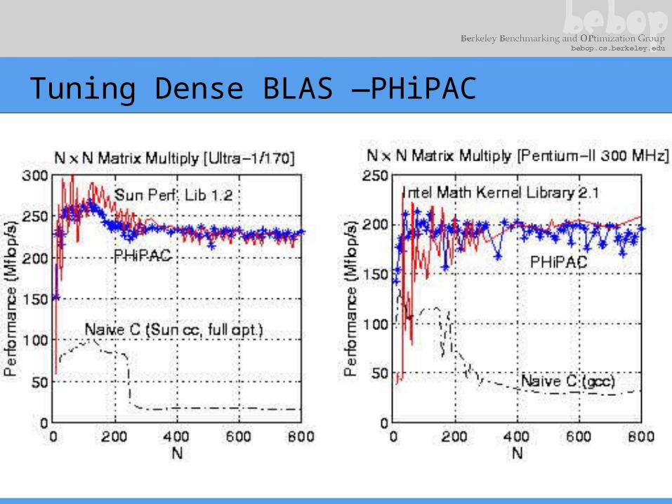
Tuning Dense BLAS —PHiPAC

Tuning Dense BLAS– ATLAS
Extends applicability of PHIPAC; Incorporated in Matlab (with rest of LAPACK)

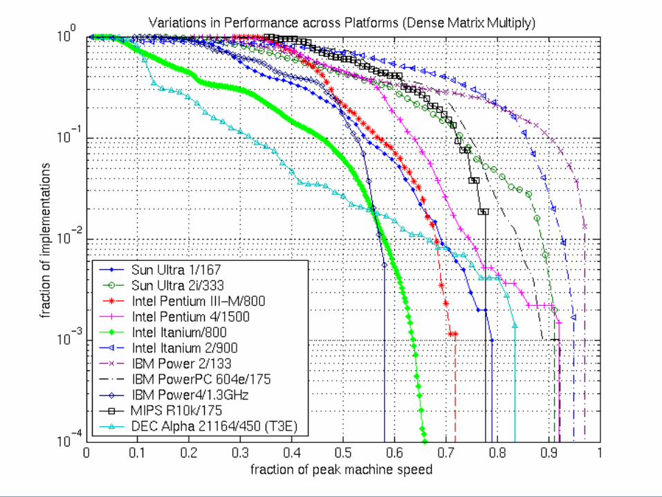
Tuning Register Tile Sizes (Dense Matrix Multiply)
333 MHz Sun Ultra 2i
2-D slice of 3-D space; implementations color-coded by performance in Mflop/s
16 registers, but 2-by-3 tile size fastest
Needle in a haystack
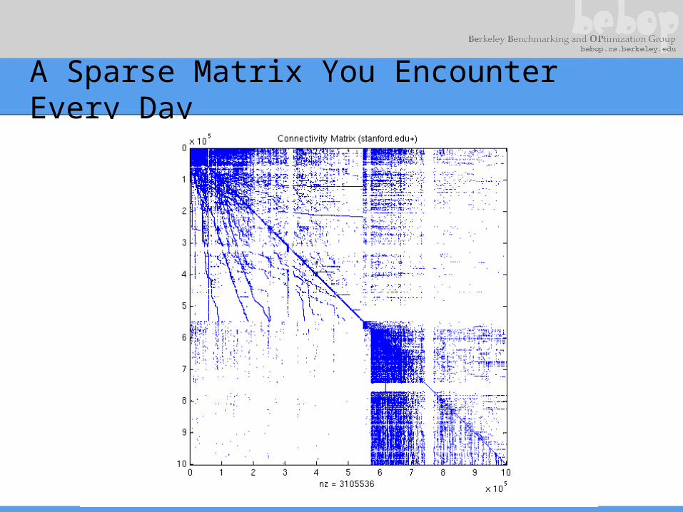
A Sparse Matrix You Encounter Every Day
Matrix-vector multiply kernel: y(i) y(i) + A(i,j)*x(j)
for each row i
for k=ptr[i] to ptr[i+1] do
y[i] = y[i] + val[k]*x[ind[k]]
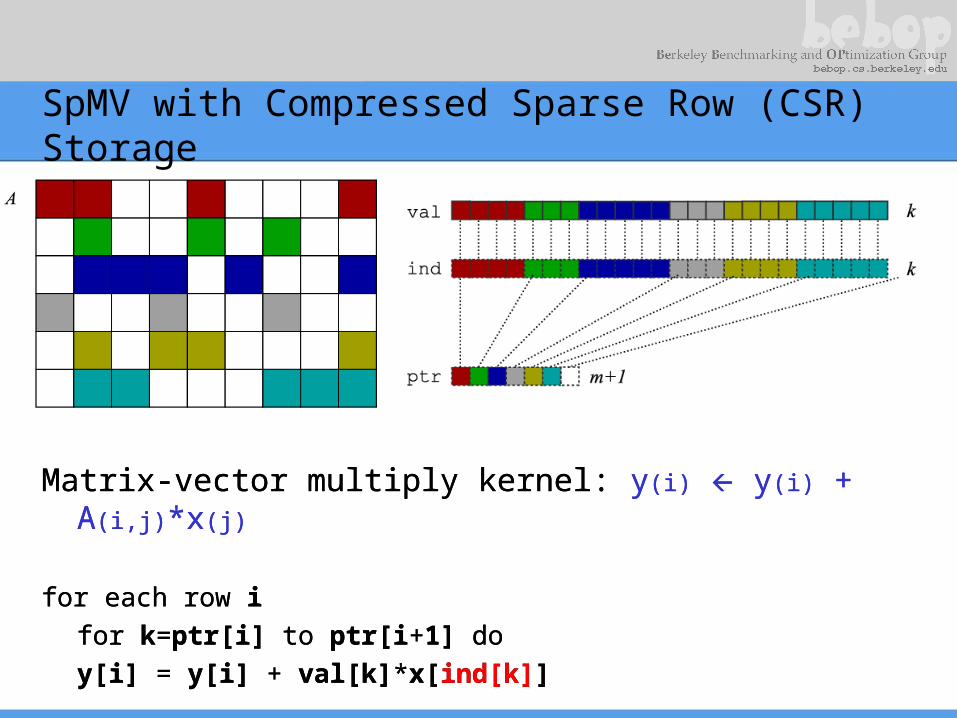
SpMV with Compressed Sparse Row (CSR) Storage
Matrix-vector multiply kernel: y(i) y(i) + A(i,j)*x(j)
for each row i
for k=ptr[i] to ptr[i+1] do
y[i] = y[i] + val[k]*x[ind[k]]
Motivation for Automatic Performance Tuning of SpMV
• Historical trends– Sparse matrix-vector multiply (SpMV): 10% of peak or
less– 2x faster than CSR with “hand-tuning”– Tuning becoming more difficult over time
• Performance depends on machine, kernel, matrix– Matrix known at run-time– Best data structure + implementation can be surprising
• Our approach: empirical modeling and search– Up to 4x speedups and 31% of peak for SpMV– Many optimization techniques for SpMV– Several other kernels: triangular solve, ATA*x, Ak*x– Release OSKI Library, integrate into PETSc

SpMV Historical Trends: Fraction of Peak
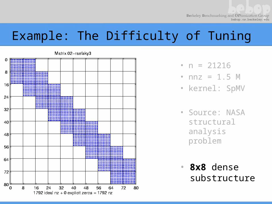
Example: The Difficulty of Tuning
• n = 21216• nnz = 1.5 M• kernel: SpMV
• Source: NASA structural analysis problem
• 8x8 dense substructure
Taking advantage of block structure in SpMV
• Bottleneck is time to get matrix from memory– Only 2 flops for each nonzero in matrix
• Don’t store each nonzero with index, instead store each nonzero r-by-c block with index– Storage drops by up to 2x, if rc >> 1, all 32-bit
quantities– Time to fetch matrix from memory decreases
• Change both data structure and algorithm– Need to pick r and c– Need to change algorithm accordingly
• In example, is r=c=8 best choice?– Minimizes storage, so looks like a good idea…

Speedups on Itanium 2: The Need for Search
Reference
Best: 4x2
Mflop/s
Mflop/s

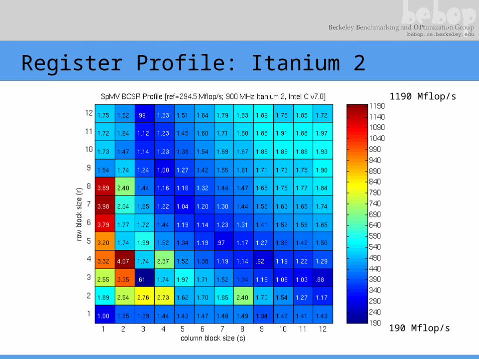
Register Profile: Itanium 2
190 Mflop/s
1190 Mflop/s
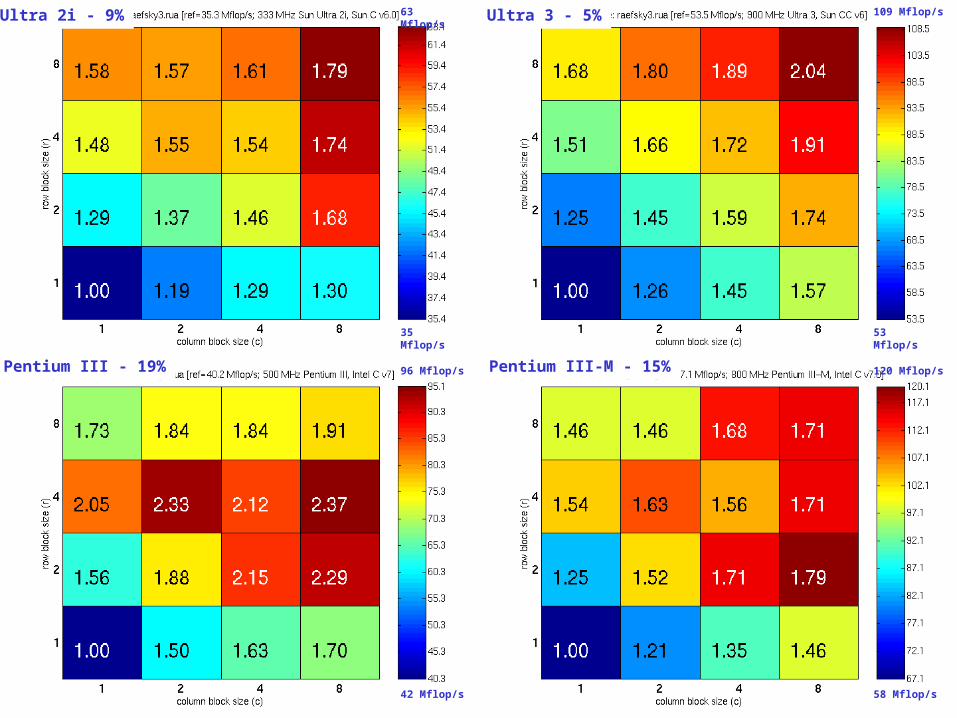
SpMV Performance (Matrix #2): Generation 2
Ultra 2i - 9% Ultra 3 - 5%
Pentium III-M - 15%Pentium III - 19%
63 Mflop/s
35 Mflop/s
109 Mflop/s
53 Mflop/s
96 Mflop/s
42 Mflop/s
120 Mflop/s
58 Mflop/s
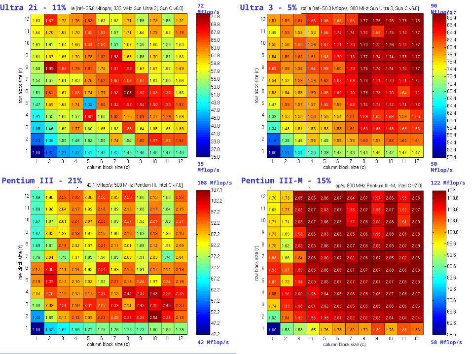
Register Profiles: Sun and Intel x86
Ultra 2i - 11% Ultra 3 - 5%
Pentium III-M - 15%Pentium III - 21%
72 Mflop/s
35 Mflop/s
90 Mflop/s
50 Mflop/s
108 Mflop/s
42 Mflop/s
122 Mflop/s
58 Mflop/s
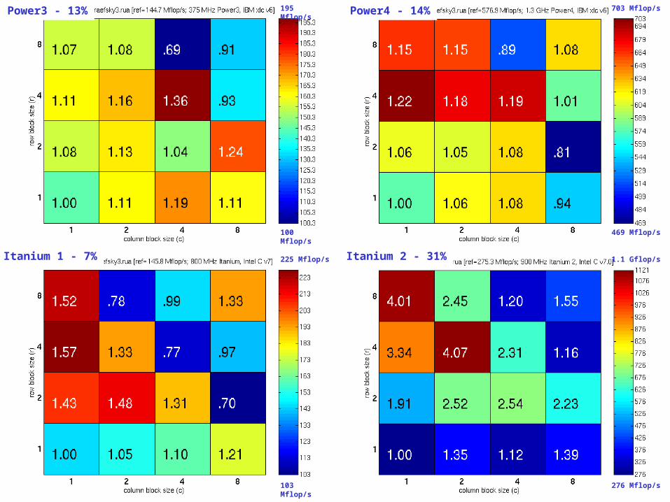
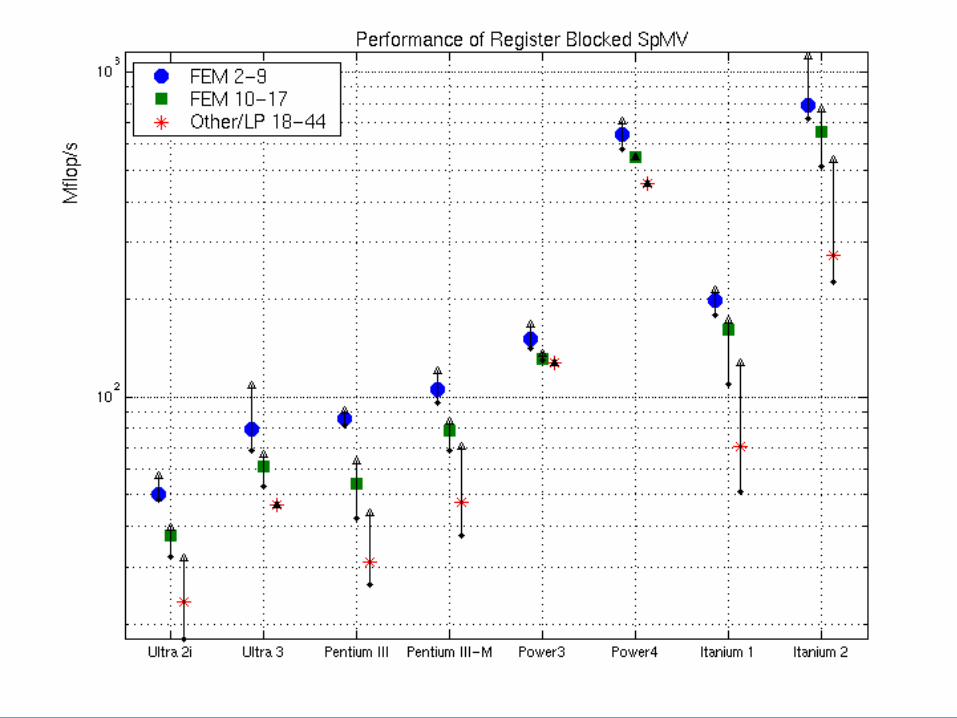
SpMV Performance (Matrix #2): Generation 1
Power3 - 13% Power4 - 14%
Itanium 2 - 31%Itanium 1 - 7%
195 Mflop/s
100 Mflop/s
703 Mflop/s
469 Mflop/s
225 Mflop/s
103 Mflop/s
1.1 Gflop/s
276 Mflop/s

Register Profiles: IBM and Intel IA-64
Power3 - 17% Power4 - 16%
Itanium 2 - 33%Itanium 1 - 8%
252 Mflop/s
122 Mflop/s
820 Mflop/s
459 Mflop/s
247 Mflop/s
107 Mflop/s
1.2 Gflop/s
190 Mflop/s

Example: The Difficulty of Tuning
• n = 21216• nnz = 1.5 M• kernel: SpMV
• Source: NASA structural analysis problem
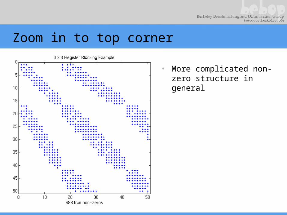
Zoom in to top corner
• More complicated non-zero structure in general

3x3 blocks look natural, but…
• More complicated non-zero structure in general
• Example: 3x3 blocking– Logical grid of 3x3 cells
• But would lead to lots of “fill-in”
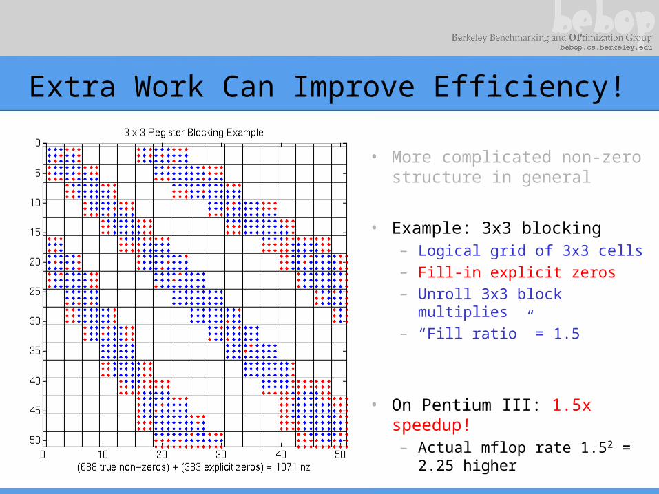
Extra Work Can Improve Efficiency!
• More complicated non-zero structure in general
• Example: 3x3 blocking– Logical grid of 3x3 cells– Fill-in explicit zeros– Unroll 3x3 block multiplies– “Fill ratio” = 1.5
• On Pentium III: 1.5x speedup!– Actual mflop rate 1.52 =
2.25 higher
Automatic Register Block Size Selection
• Selecting the r x c block size– Off-line benchmark
• Precompute Mflops(r,c) using dense A for each r x c• Once per machine/architecture
– Run-time “search”• Sample A to estimate Fill(r,c) for each r x c
– Run-time heuristic model• Choose r, c to maximize Mflops(r,c) / Fill(r,c)
Accurate and Efficient Adaptive Fill Estimation
• Idea: Sample matrix– Fraction of matrix to sample: s [0,1]– Cost ~ O(s * nnz)– Control cost by controlling s
• Search at run-time: the constant matters!
• Control s automatically by computing statistical confidence intervals– Idea: Monitor variance
• Cost of tuning– Lower bound: convert matrix in 5 to 40 unblocked
SpMVs– Heuristic: 1 to 11 SpMVs
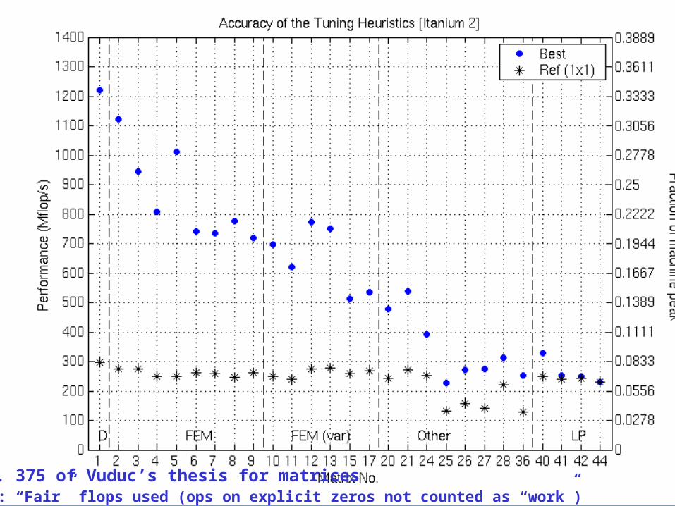
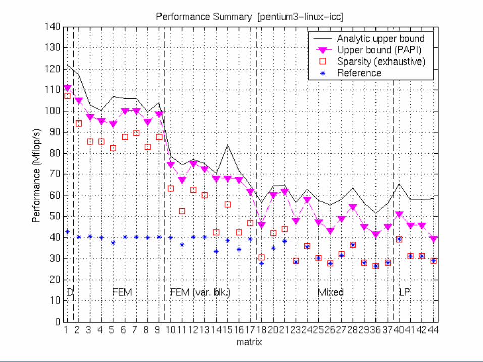
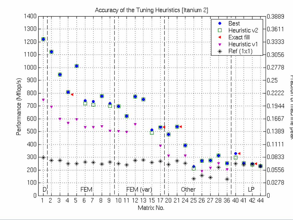
Accuracy of the Tuning Heuristics (1/4)
NOTE: “Fair” flops used (ops on explicit zeros not counted as “work”)See p. 375 of Vuduc’s thesis for matrices

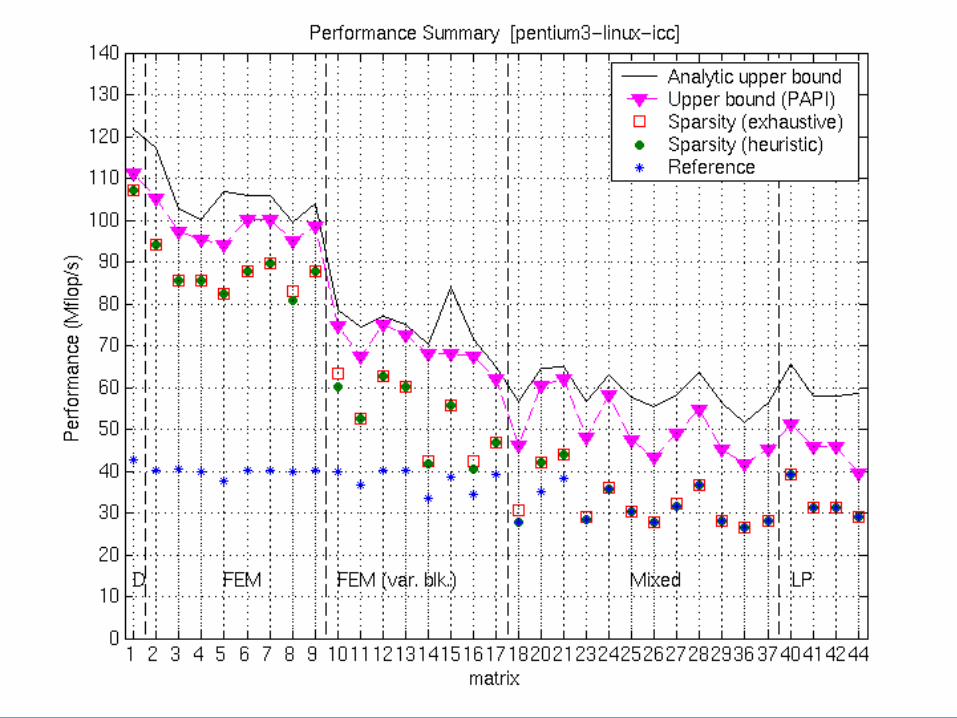
Accuracy of the Tuning Heuristics (2/4)

Accuracy of the Tuning Heuristics (3/4)
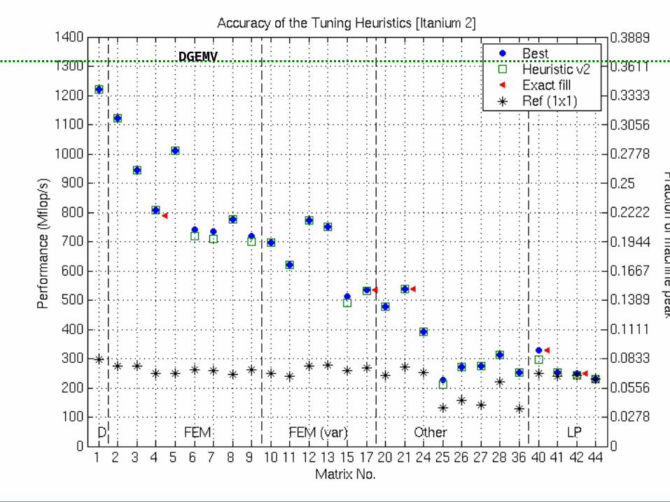
Accuracy of the Tuning Heuristics (3/4)DGEMV

Evaluating algorithms and machines for SpMV
• Metrics– Speedups– Mflop/s (“fair” flops)– Fraction of peak
• Questions– Speedups are good, but what is “the best?”
• Independent of instruction scheduling, selection• Can SpMV be further improved or not?
– What machines are “good” for SpMV?

Upper Bounds on Performance for blocked SpMV
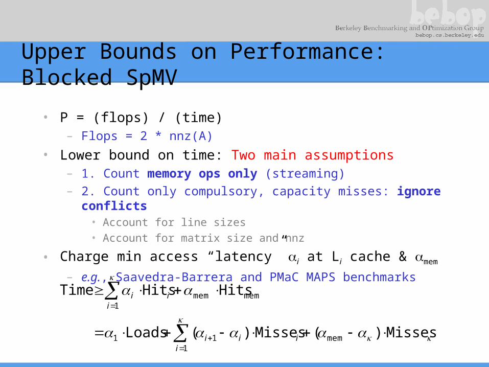
• P = (flops) / (time)– Flops = 2 * nnz(A)
• Lower bound on time: Two main assumptions– 1. Count memory ops only (streaming)– 2. Count only compulsory, capacity misses: ignore conflicts
• Account for line sizes• Account for matrix size and nnz
• Charge minimum access “latency” i at Li cache & mem
– e.g., Saavedra-Barrera and PMaC MAPS benchmarks
1mem11
1memmem
Misses)(Misses)(Loads
HitsHitsTime
iiii
iii
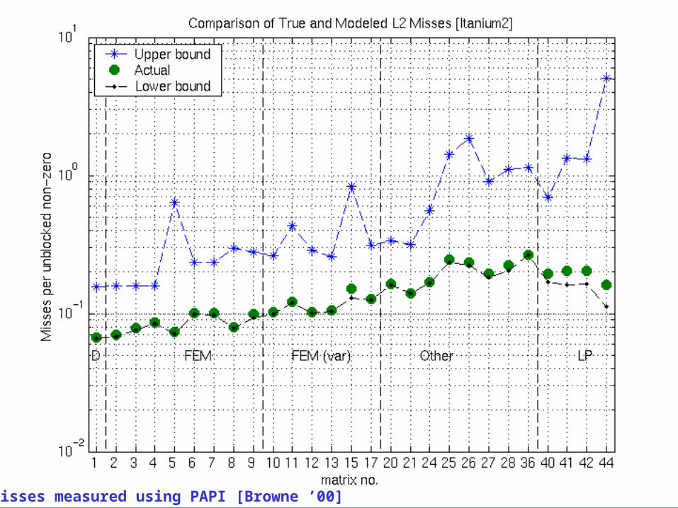
Example: L2 Misses on Itanium 2
Misses measured using PAPI [Browne ’00]
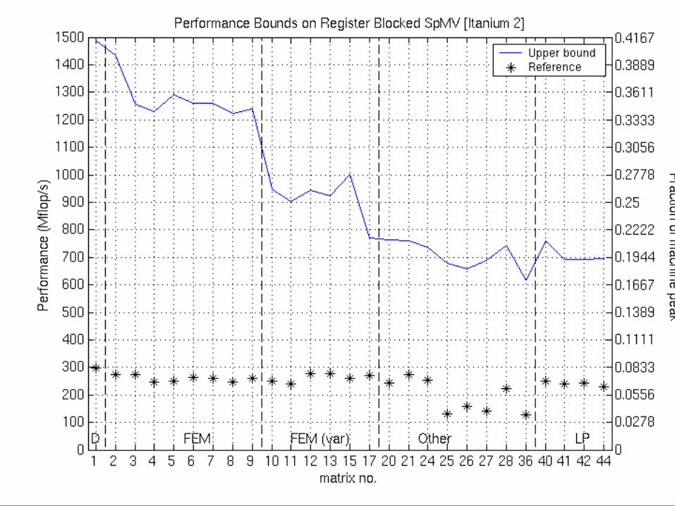
Example: Bounds on Itanium 2

Example: Bounds on Itanium 2
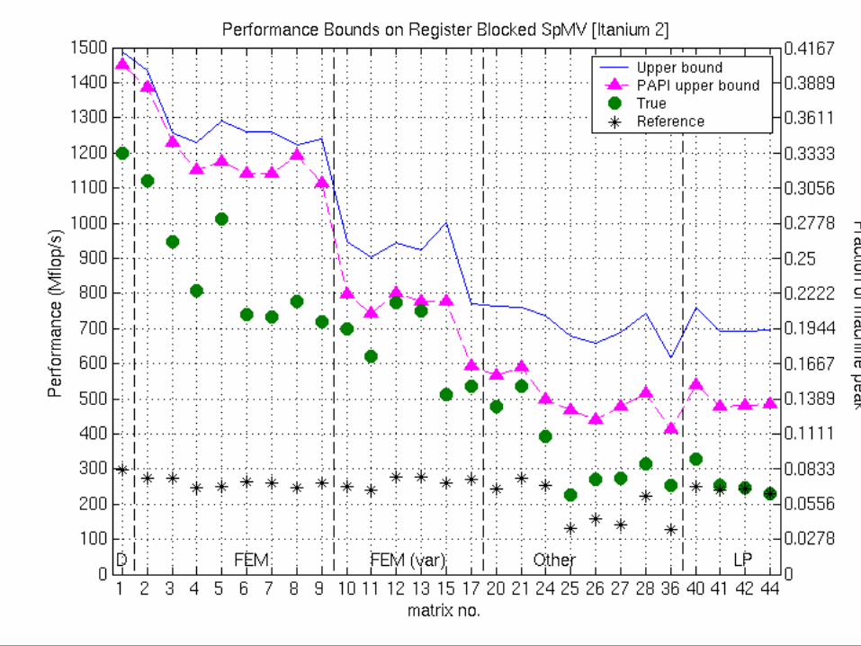
Example: Bounds on Itanium 2

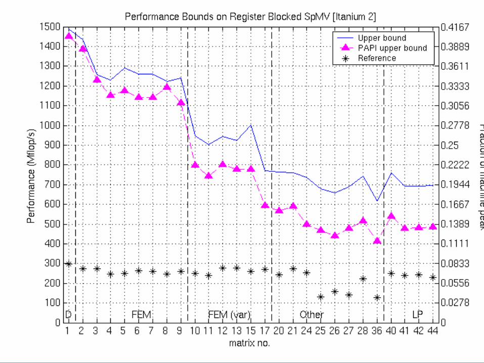
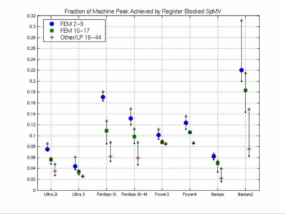
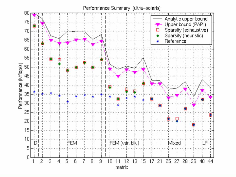
Fraction of Upper Bound Across Platforms

Achieved Performance and Machine Balance
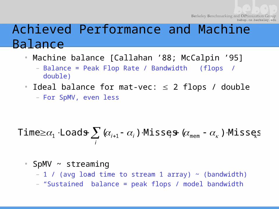
• Machine balance [Callahan ’88; McCalpin ’95]– Balance = Peak Flop Rate / Bandwidth (flops /
double)– Lower is better (I.e. can hope to get higher fraction
of peak flop rate)
• Ideal balance for mat-vec: 2 flops / double– For SpMV, even less


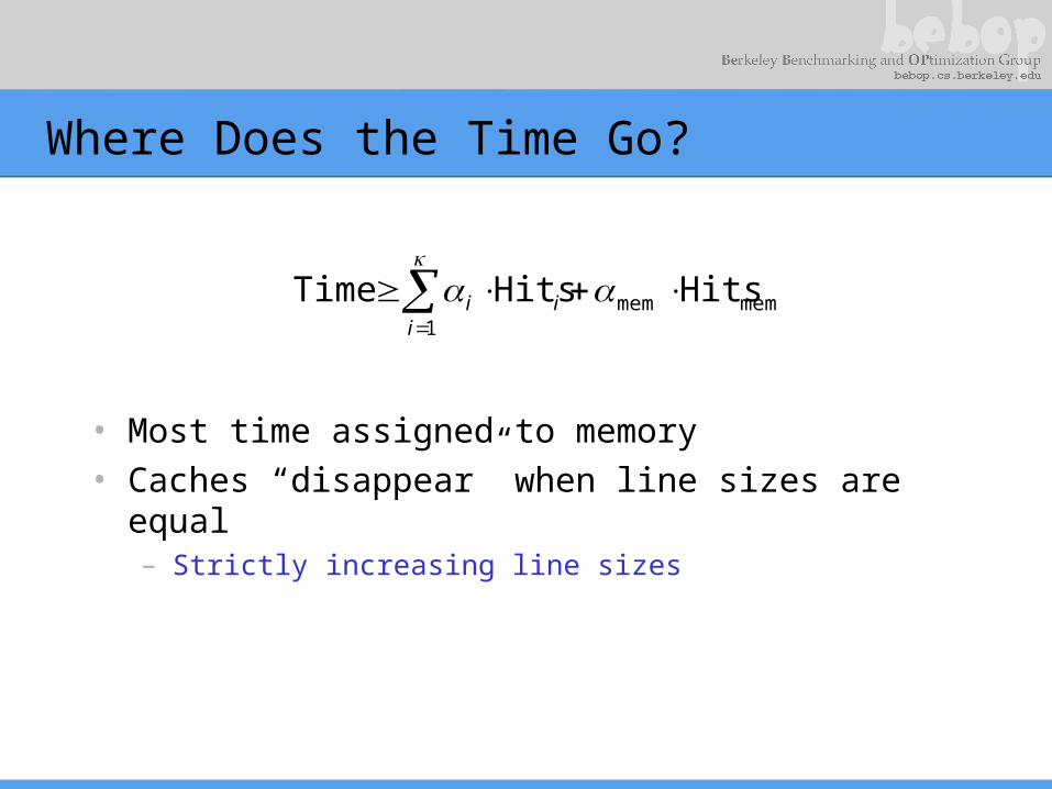
Where Does the Time Go?
• Most time assigned to memory• Caches “disappear” when line sizes are equal
– Strictly increasing line sizes
1
memmem HitsHitsTimei
ii

Execution Time Breakdown: Matrix 40

Execution Time Breakdown (PAPI): Matrix 40

Speedups with Increasing Line Size

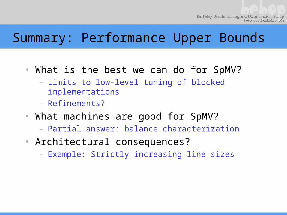
Summary: Performance Upper Bounds
• What is the best we can do for SpMV?– Limits to low-level tuning of blocked implementations– Refinements?
• What machines are good for SpMV?– Partial answer: balance characterization
• Architectural consequences?– Help to have strictly increasing line sizes

Summary of Other Performance Optimizations
• Optimizations for SpMV– Register blocking (RB): up to 4x over CSR– Variable block splitting: 2.1x over CSR, 1.8x over RB– Diagonals: 2x over CSR– Reordering to create dense structure + splitting: 2x
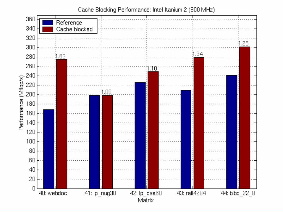
over CSR– Symmetry: 2.8x over CSR, 2.6x over RB– Cache blocking: 2.8x over CSR– Multiple vectors (SpMM): 7x over CSR– And combinations…
• Sparse triangular solve– Hybrid sparse/dense data structure: 1.8x over CSR
• Higher-level kernels– AAT*x, ATA*x: 4x over CSR, 1.8x over RB– A*x: 2x over CSR, 1.5x over RB

Example: Sparse Triangular Factor
• Raefsky4 (structural problem) + SuperLU + colmmd
• N=19779, nnz=12.6 M
Dense trailing triangle: dim=2268, 20% of total nz
Can be as high as 90+%!1.8x over CSR
Cache Optimizations for AAT*x
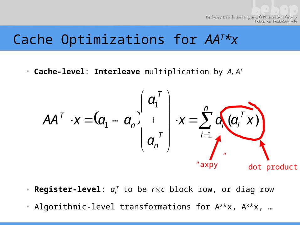
• Cache-level: Interleave multiplication by A, AT
• Register-level: aiT to be rc block row, or diag row
n
i
Tii
Tn
T
nT xaax
a
a
aaxAA1
1
1 )(
dot product“axpy”
• Algorithmic-level transformations for A2*x, A3*x, …
… …

Example: Combining Optimizations
• Register blocking, symmetry, multiple (k) vectors– Three low-level tuning parameters: r, c, v
v
kX
Y A
cr
+=
*
Example: Combining Optimizations
• Register blocking, symmetry, and multiple vectors [Ben Lee @ UCB]– Symmetric, blocked, 1 vector
• Up to 2.6x over nonsymmetric, blocked, 1 vector
– Symmetric, blocked, k vectors• Up to 2.1x over nonsymmetric, blocked, k vecs.• Up to 7.3x over nonsymmetric, nonblocked, 1, vector
– Symmetric Storage: 64.7% savings

Potential Impact on Applications: T3P
• Application: accelerator design [Ko] • 80% of time spent in SpMV• Relevant optimization techniques
– Symmetric storage– Register blocking
• On Single Processor Itanium 2– 1.68x speedup
• 532 Mflops, or 15% of 3.6 GFlop peak– 4.4x speedup with multiple (8) vectors
• 1380 Mflops, or 38% of peak
Potential Impact on Applications: Omega3P
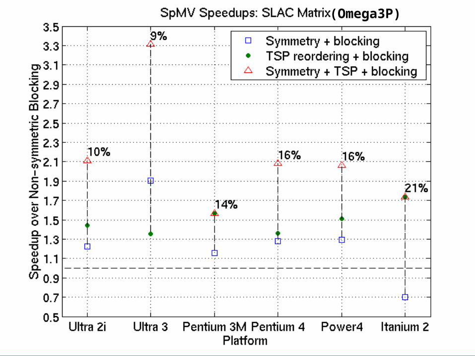
• Application: accelerator cavity design [Ko]• Relevant optimization techniques
– Symmetric storage– Register blocking– Reordering
• Reverse Cuthill-McKee ordering to reduce bandwidth• Traveling Salesman Problem-based ordering to create
blocks– Nodes = columns of A– Weights(u, v) = no. of nz u, v have in common– Tour = ordering of columns– Choose maximum weight tour– See [Pinar & Heath ’97]
• 2.1x speedup on Power 4, but SPMV not dominant

Source: Accelerator Cavity Design Problem (Ko via Husbands)

100x100 Submatrix Along Diagonal

Post-RCM Reordering

Before: Green + RedAfter: Green + Blue
“Microscopic” Effect of RCM Reordering

“Microscopic” Effect of Combined RCM+TSP Reordering
Before: Green + RedAfter: Green + Blue
(Omega3P)
Optimized Sparse Kernel Interface - OSKI
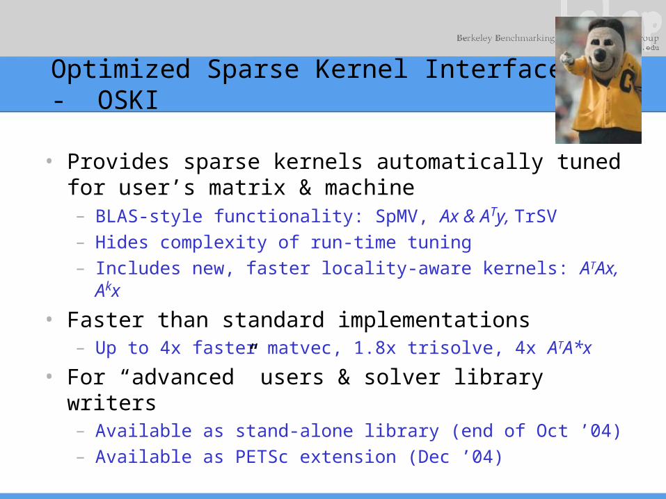
• Provides sparse kernels automatically tuned for user’s matrix & machine– BLAS-style functionality: SpMV, Ax & ATy, TrSV– Hides complexity of run-time tuning– Includes new, faster locality-aware kernels: ATAx, Akx
• Faster than standard implementations– Up to 4x faster matvec, 1.8x trisolve, 4x ATA*x
• For “advanced” users & solver library writers– Available as stand-alone library (end of Oct ’04)– Available as PETSc extension (Dec ’04)

How the OSKI Tunes (Overview)
Benchmarkdata
1. Build forTargetArch.
2. Benchmark
Heuristicmodels
1. EvaluateModels
Generatedcode
variants
2. SelectData Struct.
& Code
Library Install-Time (offline) Application Run-Time
To user:Matrix handlefor kernelcalls
Workloadfrom program
monitoring
Extensibility: Advanced users may write & dynamically add “Code variants” and “Heuristic models” to system.
HistoryMatrix

How the OSKI Tunes (Overview)
• At library build/install-time– Pre-generate and compile code variants into dynamic
libraries– Collect benchmark data
• Measures and records speed of possible sparse data structure and code variants on target architecture
– Installation process uses standard, portable GNU AutoTools• At run-time
– Library “tunes” using heuristic models• Models analyze user’s matrix & benchmark data to choose
optimized data structure and code– Non-trivial tuning cost: up to ~40 mat-vecs
• Library limits the time it spends tuning based on estimated workload
– provided by user or inferred by library• User may reduce cost by saving tuning results for application
on future runs with same or similar matrix

Optimizations in the Initial OSKI Release
• Fully automatic heuristics for– Sparse matrix-vector multiply
• Register-level blocking• Register-level blocking + symmetry + multiple vectors• Cache-level blocking
– Sparse triangular solve with register-level blocking and “switch-to-dense” optimization
– Sparse ATA*x with register-level blocking• User may select other optimizations manually
– Diagonal storage optimizations, reordering, splitting; tiled matrix powers kernel (Ak*x)
– All available in dynamic libraries– Accessible via high-level embedded script language
• “Plug-in” extensibility– Very advanced users may write their own heuristics, create new
data structures/code variants and dynamically add them to the system
Statistical Models for Automatic Tuning
• Idea 1: Statistical criterion for stopping a search– A general search model
• Generate implementation• Measure performance• Repeat
– Stop when probability of being within of optimal falls below threshold
• Can estimate distribution on-line
• Idea 2: Statistical performance models– Problem: Choose 1 among m implementations at run-
time– Sample performance off-line, build statistical model
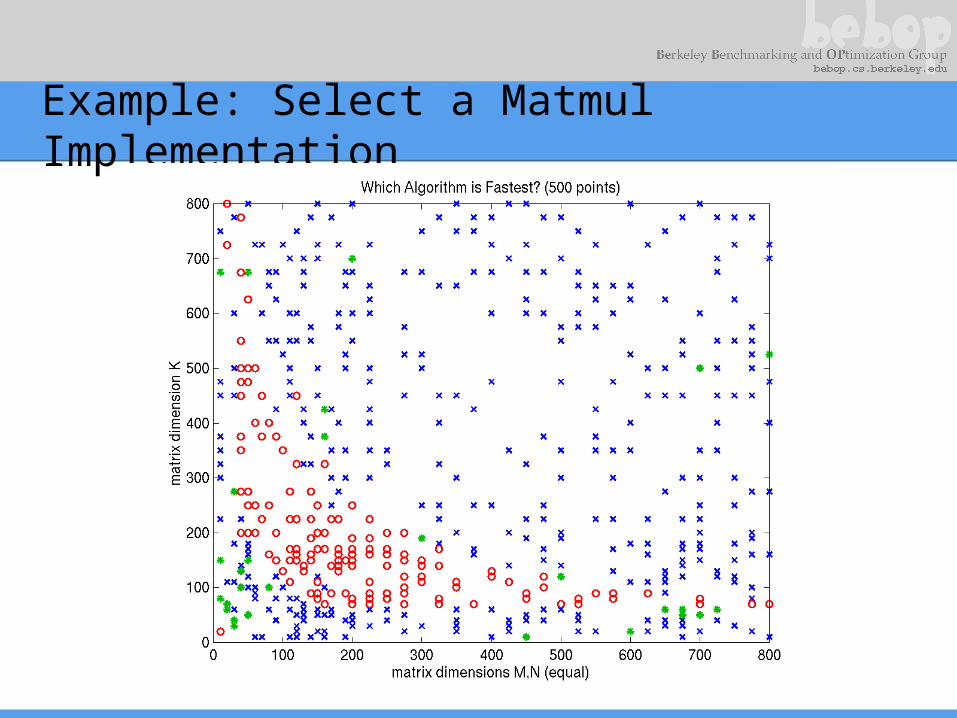
Example: Select a Matmul Implementation

Example: Support Vector Classification

A Sparse Matrix You Encounter Every Day
Who am I?
I am aBig Repository
Of usefulAnd uselessFacts alike.
Who am I?
(Hint: Not your e-mail inbox.)
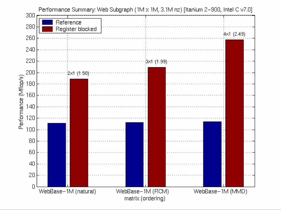
What about the Google Matrix?
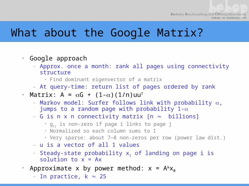
• Google approach– Approx. once a month: rank all pages using connectivity
structure• Find dominant eigenvector of a matrix
– At query-time: return list of pages ordered by rank• Matrix: A = G + (1-)(1/n)uuT
– Markov model: Surfer follows link with probability , jumps to a random page with probability 1-
– G is n x n connectivity matrix [n billions]• gij is non-zero if page i links to page j• Normalized so each column sums to 1• Very sparse: about 7—8 non-zeros per row (power law dist.)
– u is a vector of all 1 values– Steady-state probability xi of landing on page i is solution to x
= Ax
• Approximate x by power method: x = Akx0
– In practice, k 25

Extra Slides

Current Work
• Public software release• Impact on library designs: Sparse BLAS, Trilinos, PETSc,
…• Integration in large-scale applications
– DOE: Accelerator design; plasma physics– Geophysical simulation based on Block Lanczos (ATA*X; LBL)
• Systematic heuristics for data structure selection?• Evaluation of emerging architectures
– Revisiting vector micros
• Other sparse kernels– Matrix triple products, Ak*x
• Parallelism• Sparse benchmarks (with UTK) [Gahvari & Hoemmen]• Automatic tuning of MPI collective ops [Nishtala, et al.]
Summary of High-Level Themes
• “Kernel-centric” optimization– Vs. basic block, trace, path optimization, for instance– Aggressive use of domain-specific knowledge
• Performance bounds modeling– Evaluating software quality– Architectural characterizations and consequences
• Empirical search– Hybrid on-line/run-time models
• Statistical performance models– Exploit information from sampling, measuring
Related Work
• My bibliography: 337 entries so far• Sample area 1: Code generation
– Generative & generic programming– Sparse compilers– Domain-specific generators
• Sample area 2: Empirical search-based tuning– Kernel-centric
• linear algebra, signal processing, sorting, MPI, …
– Compiler-centric• profiling + FDO, iterative compilation, superoptimizers,
self-tuning compilers, continuous program optimization
Future Directions (A Bag of Flaky Ideas)
• Composable code generators and search spaces• New application domains
– PageRank: multilevel block algorithms for topic-sensitive search?
• New kernels: cryptokernels– rich mathematical structure germane to performance; lots
of hardware
• New tuning environments– Parallel, Grid, “whole systems”
• Statistical models of application performance– Statistical learning of concise parametric models from
traces for architectural evaluation– Compiler/automatic derivation of parametric models
Possible Future Work
• Different Architectures– New FP instruction sets (SSE2)– SMP / multicore platforms– Vector architectures
• Different Kernels• Higher Level Algorithms
– Parallel versions of kenels, with optimized communication– Block algorithms (eg Lanczos)– XBLAS (extra precision)
• Produce Benchmarks– Augment HPCC Benchmark
• Make it possible to combine optimizations easily for any kernel
• Related tuning activities (LAPACK & ScaLAPACK)

Review of Tuning by Illustration
(Extra Slides)

Splitting for Variable Blocks and Diagonals
• Decompose A = A1 + A2 + … At
– Detect “canonical” structures (sampling)– Split
– Tune each Ai
– Improve performance and save storage
• New data structures– Unaligned block CSR
• Relax alignment in rows & columns
– Row-segmented diagonals

Example: Variable Block Row (Matrix #12)
2.1x over CSR1.8x over RB

Example: Row-Segmented Diagonals
2x over CSR
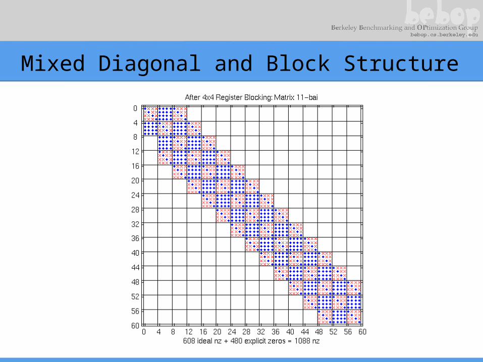
Mixed Diagonal and Block Structure

Summary
• Automated block size selection– Empirical modeling and search– Register blocking for SpMV, triangular solve, ATA*x
• Not fully automated– Given a matrix, select splittings and transformations
• Lots of combinatorial problems– TSP reordering to create dense blocks (Pinar ’97;
Moon, et al. ’04)
Extra Slides

A Sparse Matrix You Encounter Every Day
Who am I?
I am aBig Repository
Of usefulAnd uselessFacts alike.
Who am I?
(Hint: Not your e-mail inbox.)
Problem Context
• Sparse kernels abound– Models of buildings, cars, bridges, economies, …– Google PageRank algorithm
• Historical trends– Sparse matrix-vector multiply (SpMV): 10% of peak– 2x faster with “hand-tuning”– Tuning becoming more difficult over time– Promise of automatic tuning: PHiPAC/ATLAS, FFTW, …
• Challenges to high-performance– Not dense linear algebra!
• Complex data structures: indirect, irregular memory access
• Performance depends strongly on run-time inputs

Key Questions, Ideas, Conclusions
• How to tune basic sparse kernels automatically?– Empirical modeling and search
• Up to 4x speedups for SpMV• 1.8x for triangular solve• 4x for ATA*x; 2x for A2*x• 7x for multiple vectors
• What are the fundamental limits on performance?– Kernel-, machine-, and matrix-specific upper bounds
• Achieve 75% or more for SpMV, limiting low-level tuning• Consequences for architecture?
• General techniques for empirical search-based tuning?– Statistical models of performance

Road Map
• Sparse matrix-vector multiply (SpMV) in a nutshell• Historical trends and the need for search• Automatic tuning techniques• Upper bounds on performance• Statistical models of performance

Matrix-vector multiply kernel: y(i) y(i) + A(i,j)*x(j)Matrix-vector multiply kernel: y(i) y(i) + A(i,j)*x(j)
for each row i
for k=ptr[i] to ptr[i+1] do
y[i] = y[i] + val[k]*x[ind[k]]
Compressed Sparse Row (CSR) Storage
Matrix-vector multiply kernel: y(i) y(i) + A(i,j)*x(j)
for each row i
for k=ptr[i] to ptr[i+1] do
y[i] = y[i] + val[k]*x[ind[k]]

Road Map
• Sparse matrix-vector multiply (SpMV) in a nutshell• Historical trends and the need for search• Automatic tuning techniques• Upper bounds on performance• Statistical models of performance
Historical Trends in SpMV Performance
• The Data– Uniprocessor SpMV performance since 1987– “Untuned” and “Tuned” implementations– Cache-based superscalar micros; some vectors– LINPACK

SpMV Historical Trends: Mflop/s

Example: The Difficulty of Tuning
• n = 21216• nnz = 1.5 M• kernel: SpMV
• Source: NASA structural analysis problem

Still More Surprises
• More complicated non-zero structure in general

Still More Surprises
• More complicated non-zero structure in general
• Example: 3x3 blocking– Logical grid of 3x3 cells
Historical Trends: Mixed News
• Observations– Good news: Moore’s law like behavior– Bad news: “Untuned” is 10% peak or less,
worsening– Good news: “Tuned” roughly 2x better today, and
improving– Bad news: Tuning is complex
– (Not really news: SpMV is not LINPACK)
• Questions– Application: Automatic tuning?– Architect: What machines are good for SpMV?

Road Map
• Sparse matrix-vector multiply (SpMV) in a nutshell• Historical trends and the need for search• Automatic tuning techniques
– SpMV [SC’02; IJHPCA ’04b]– Sparse triangular solve (SpTS) [ICS/POHLL ’02]– ATA*x [ICCS/WoPLA ’03]
• Upper bounds on performance• Statistical models of performance
SPARSITY: Framework for Tuning SpMV
• SPARSITY: Automatic tuning for SpMV [Im & Yelick ’99]– General approach
• Identify and generate implementation space• Search space using empirical models & experiments
– Prototype library and heuristic for choosing register block size
• Also: cache-level blocking, multiple vectors
• What’s new?– New block size selection heuristic
• Within 10% of optimal — replaces previous version
– Expanded implementation space• Variable block splitting, diagonals, combinations
– New kernels: sparse triangular solve, ATA*x, A*x

Automatic Register Block Size Selection
• Selecting the r x c block size– Off-line benchmark: characterize the machine
• Precompute Mflops(r,c) using dense matrix for each r x c• Once per machine/architecture
– Run-time “search”: characterize the matrix• Sample A to estimate Fill(r,c) for each r x c
– Run-time heuristic model• Choose r, c to maximize Mflops(r,c) / Fill(r,c)
• Run-time costs– Up to ~40 SpMVs (empirical worst case)

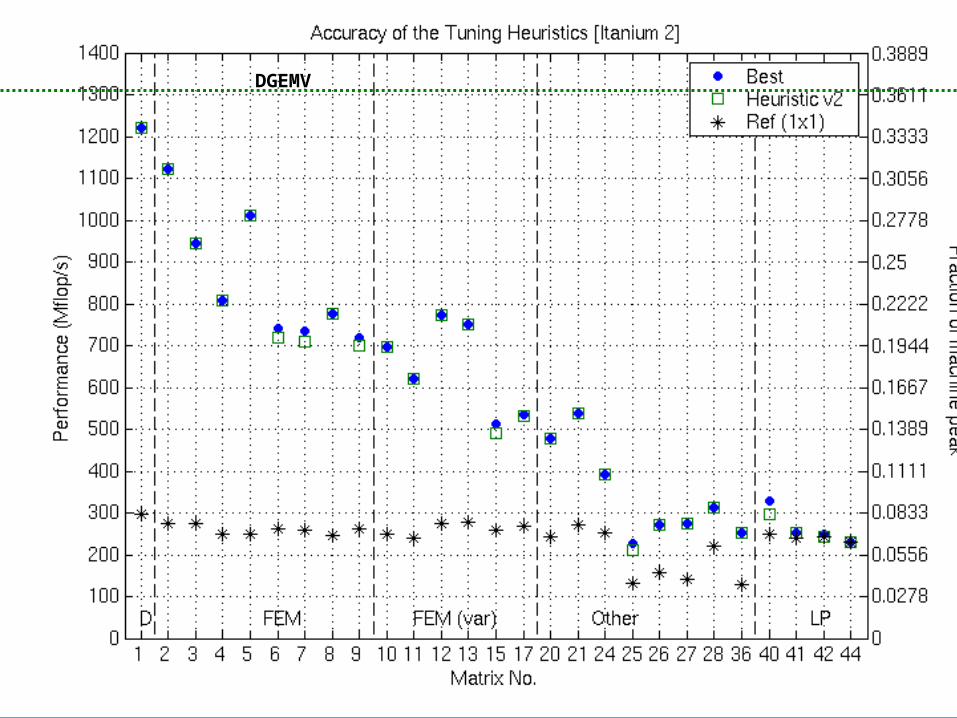
Accuracy of the Tuning Heuristics (1/4)
NOTE: “Fair” flops used (ops on explicit zeros not counted as “work”)
DGEMV
Accuracy of the Tuning Heuristics (2/4)DGEMV

Accuracy of the Tuning Heuristics (3/4)DGEMV

Accuracy of the Tuning Heuristics (4/4)DGEMV

Road Map
• Sparse matrix-vector multiply (SpMV) in a nutshell• Historical trends and the need for search• Automatic tuning techniques• Upper bounds on performance
– SC’02
• Statistical models of performance
Motivation for Upper Bounds Model
• Questions– Speedups are good, but what is the speed limit?
• Independent of instruction scheduling, selection
– What machines are “good” for SpMV?
Upper Bounds on Performance: Blocked SpMV
• P = (flops) / (time)– Flops = 2 * nnz(A)
• Lower bound on time: Two main assumptions– 1. Count memory ops only (streaming)– 2. Count only compulsory, capacity misses: ignore conflicts
• Account for line sizes• Account for matrix size and nnz
• Charge min access “latency” i at Li cache & mem
– e.g., Saavedra-Barrera and PMaC MAPS benchmarks
1mem11
1memmem
Misses)(Misses)(Loads
HitsHitsTime
iiii
iii

Example: Bounds on Itanium 2
Example: Bounds on Itanium 2

Example: Bounds on Itanium 2

Fraction of Upper Bound Across Platforms
Achieved Performance and Machine Balance
• Machine balance [Callahan ’88; McCalpin ’95]– Balance = Peak Flop Rate / Bandwidth (flops /
double)
• Ideal balance for mat-vec: 2 flops / double– For SpMV, even less
• SpMV ~ streaming– 1 / (avg load time to stream 1 array) ~ (bandwidth)– “Sustained” balance = peak flops / model bandwidth
i
iii Misses)(Misses)(LoadsTime mem11

Where Does the Time Go?
• Most time assigned to memory• Caches “disappear” when line sizes are equal
– Strictly increasing line sizes
1
memmem HitsHitsTimei
ii
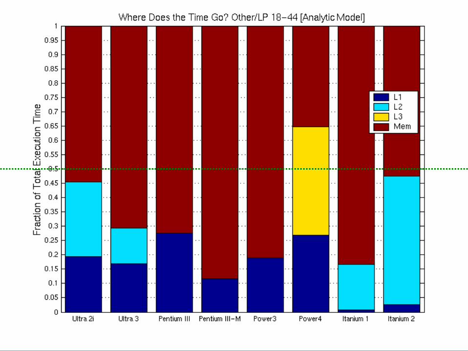
Execution Time Breakdown: Matrix 40

Speedups with Increasing Line Size
Summary: Performance Upper Bounds
• What is the best we can do for SpMV?– Limits to low-level tuning of blocked implementations– Refinements?
• What machines are good for SpMV?– Partial answer: balance characterization
• Architectural consequences?– Example: Strictly increasing line sizes

Road Map
• Sparse matrix-vector multiply (SpMV) in a nutshell• Historical trends and the need for search• Automatic tuning techniques• Upper bounds on performance• Tuning other sparse kernels• Statistical models of performance
– FDO ’00; IJHPCA ’04a

Statistical Models for Automatic Tuning
• Idea 1: Statistical criterion for stopping a search– A general search model
• Generate implementation• Measure performance• Repeat
– Stop when probability of being within of optimal falls below threshold
• Can estimate distribution on-line
• Idea 2: Statistical performance models– Problem: Choose 1 among m implementations at run-
time– Sample performance off-line, build statistical model

Example: Select a Matmul Implementation
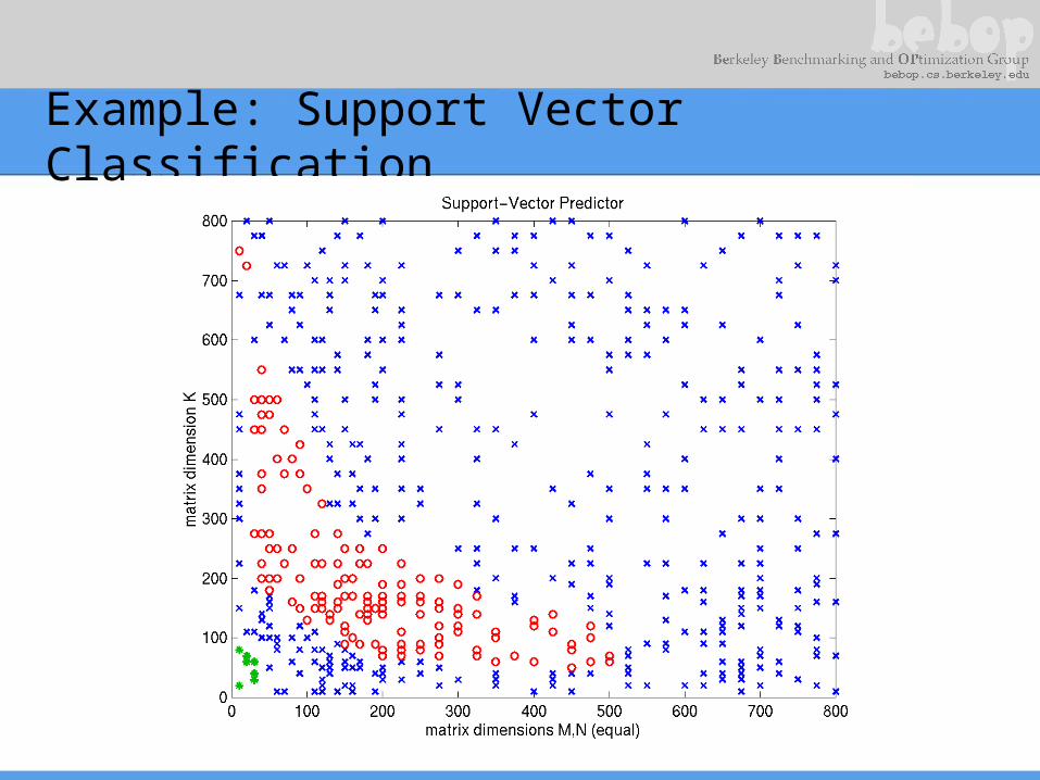
Example: Support Vector Classification

Road Map
• Sparse matrix-vector multiply (SpMV) in a nutshell• Historical trends and the need for search• Automatic tuning techniques• Upper bounds on performance• Tuning other sparse kernels• Statistical models of performance• Summary and Future Work

Summary of High-Level Themes
• “Kernel-centric” optimization– Vs. basic block, trace, path optimization, for instance– Aggressive use of domain-specific knowledge
• Performance bounds modeling– Evaluating software quality– Architectural characterizations and consequences
• Empirical search– Hybrid on-line/run-time models
• Statistical performance models– Exploit information from sampling, measuring

Related Work
• My bibliography: 337 entries so far• Sample area 1: Code generation
– Generative & generic programming– Sparse compilers– Domain-specific generators
• Sample area 2: Empirical search-based tuning– Kernel-centric
• linear algebra, signal processing, sorting, MPI, …
– Compiler-centric• profiling + FDO, iterative compilation, superoptimizers,
self-tuning compilers, continuous program optimization

Future Directions (A Bag of Flaky Ideas)
• Composable code generators and search spaces• New application domains
– PageRank: multilevel block algorithms for topic-sensitive search?
• New kernels: cryptokernels– rich mathematical structure germane to performance; lots
of hardware
• New tuning environments– Parallel, Grid, “whole systems”
• Statistical models of application performance– Statistical learning of concise parametric models from
traces for architectural evaluation– Compiler/automatic derivation of parametric models

Acknowledgements
• Super-advisors: Jim and Kathy• Undergraduate R.A.s: Attila, Ben, Jen, Jin,
Michael, Rajesh, Shoaib, Sriram, Tuyet-Linh• See pages xvi—xvii of dissertation.

TSP-based Reordering: Before
(Pinar ’97;Moon, et al ‘04)
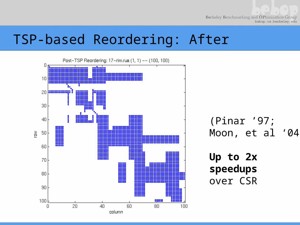
TSP-based Reordering: After
(Pinar ’97;Moon, et al ‘04)
Up to 2xspeedupsover CSR

Example: L2 Misses on Itanium 2
Misses measured using PAPI [Browne ’00]

Example: Distribution of Blocked Non-Zeros
Register Profile: Itanium 2
190 Mflop/s
1190 Mflop/s

Register Profiles: Sun and Intel x86
Ultra 2i - 11% Ultra 3 - 5%
Pentium III-M - 15%Pentium III - 21%
72 Mflop/s
35 Mflop/s
90 Mflop/s
50 Mflop/s
108 Mflop/s
42 Mflop/s
122 Mflop/s
58 Mflop/s

Register Profiles: IBM and Intel IA-64
Power3 - 17% Power4 - 16%
Itanium 2 - 33%Itanium 1 - 8%
252 Mflop/s
122 Mflop/s
820 Mflop/s
459 Mflop/s
247 Mflop/s
107 Mflop/s
1.2 Gflop/s
190 Mflop/s

Accurate and Efficient Adaptive Fill Estimation
• Idea: Sample matrix– Fraction of matrix to sample: s [0,1]– Cost ~ O(s * nnz)– Control cost by controlling s
• Search at run-time: the constant matters!
• Control s automatically by computing statistical confidence intervals– Idea: Monitor variance
• Cost of tuning– Lower bound: convert matrix in 5 to 40 unblocked
SpMVs– Heuristic: 1 to 11 SpMVs
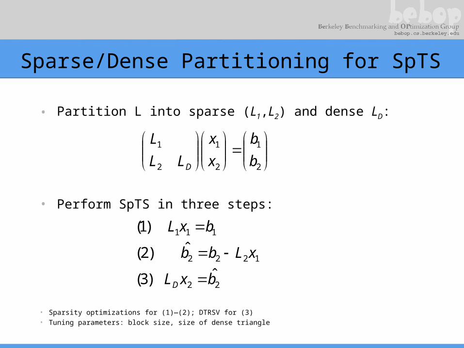
Sparse/Dense Partitioning for SpTS
• Partition L into sparse (L1,L2) and dense LD:
2
1
2
1
2
1
b
b
x
x
LL
L
D
• Perform SpTS in three steps:
22
1222
111
ˆ)3(
ˆ)2(
)1(
bxL
xLbb
bxL
D
• Sparsity optimizations for (1)—(2); DTRSV for (3)• Tuning parameters: block size, size of dense triangle

SpTS Performance: Power3
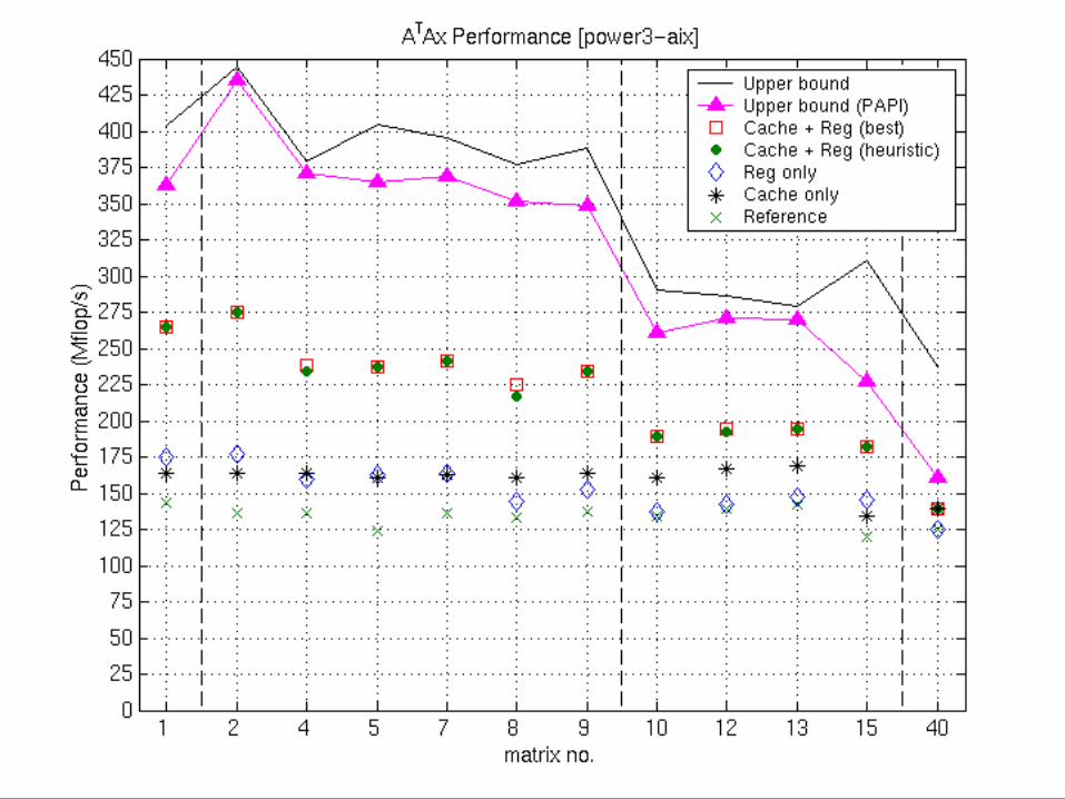
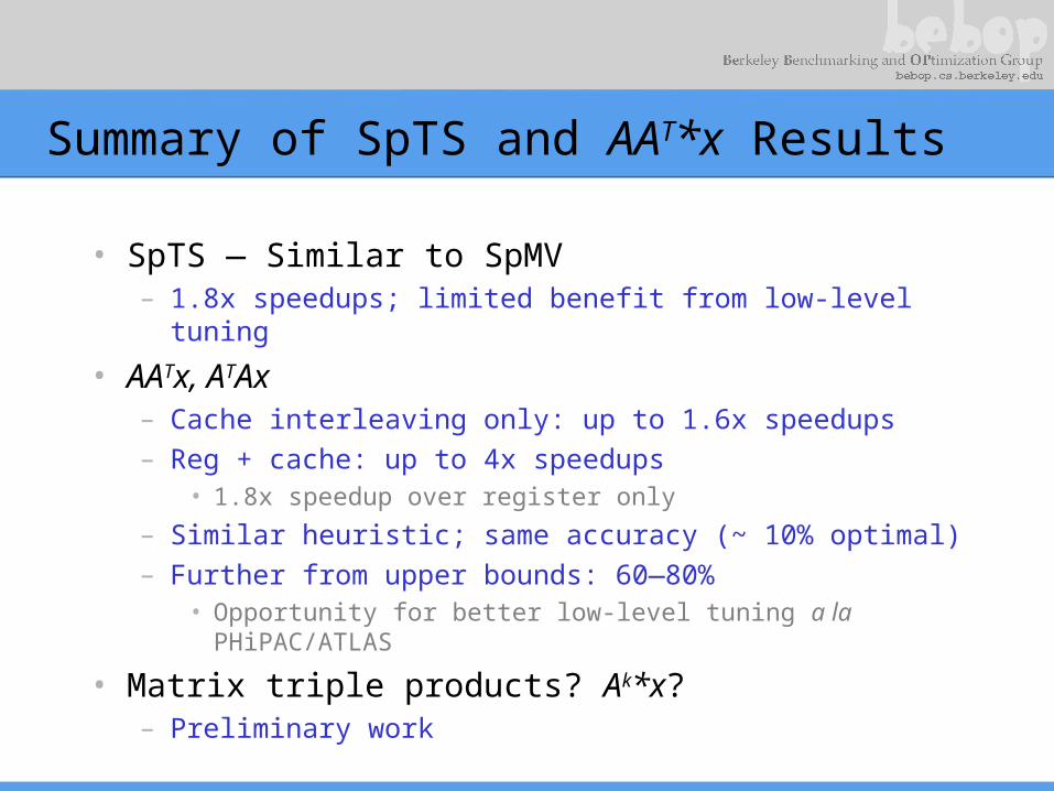
Summary of SpTS and AAT*x Results
• SpTS — Similar to SpMV– 1.8x speedups; limited benefit from low-level tuning
• AATx, ATAx– Cache interleaving only: up to 1.6x speedups– Reg + cache: up to 4x speedups
• 1.8x speedup over register only
– Similar heuristic; same accuracy (~ 10% optimal)– Further from upper bounds: 60—80%
• Opportunity for better low-level tuning a la PHiPAC/ATLAS
• Matrix triple products? Ak*x?– Preliminary work

Register Blocking: Speedup
Register Blocking: Performance
Register Blocking: Fraction of Peak

Example: Confidence Interval Estimation
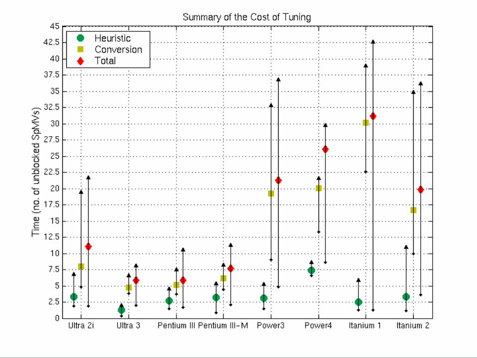
Costs of Tuning
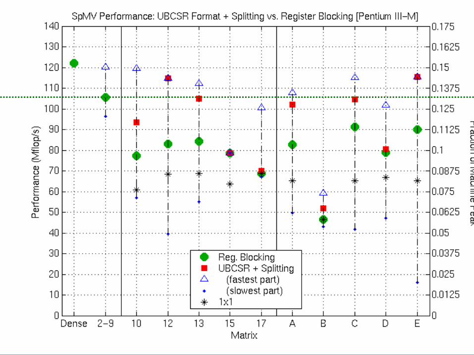
Splitting + UBCSR: Pentium III

Splitting + UBCSR: Power4

Splitting+UBCSR Storage: Power4


Example: Variable Block Row (Matrix #13)

Dense Tuning is Hard, Too
• Even dense matrix multiply can be notoriously difficult to tune

Dense matrix multiply: surprising performance as register tile size varies.


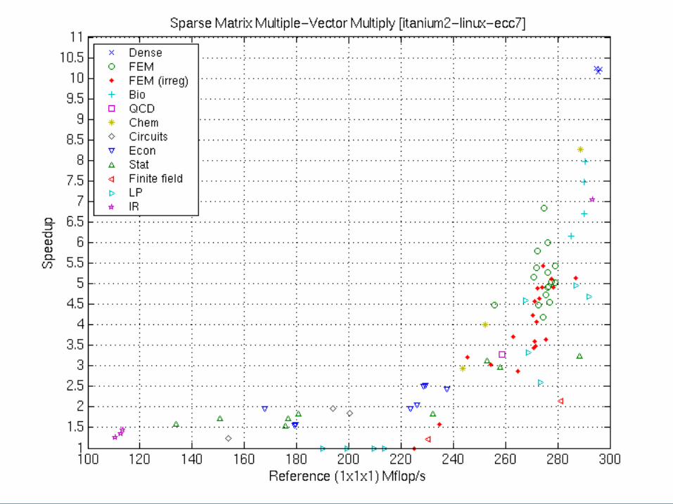
Preliminary Results (Matrix Set 2): Itanium 2
Web/IR
Dense FEM FEM (var) Bio LPEcon Stat
Multiple Vector Performance

What about the Google Matrix?
• Google approach– Approx. once a month: rank all pages using connectivity
structure• Find dominant eigenvector of a matrix
– At query-time: return list of pages ordered by rank• Matrix: A = G + (1-)(1/n)uuT
– Markov model: Surfer follows link with probability , jumps to a random page with probability 1-
– G is n x n connectivity matrix [n 3 billion]• gij is non-zero if page i links to page j• Normalized so each column sums to 1• Very sparse: about 7—8 non-zeros per row (power law dist.)
– u is a vector of all 1 values– Steady-state probability xi of landing on page i is solution to x
= Ax
• Approximate x by power method: x = Akx0
– In practice, k 25
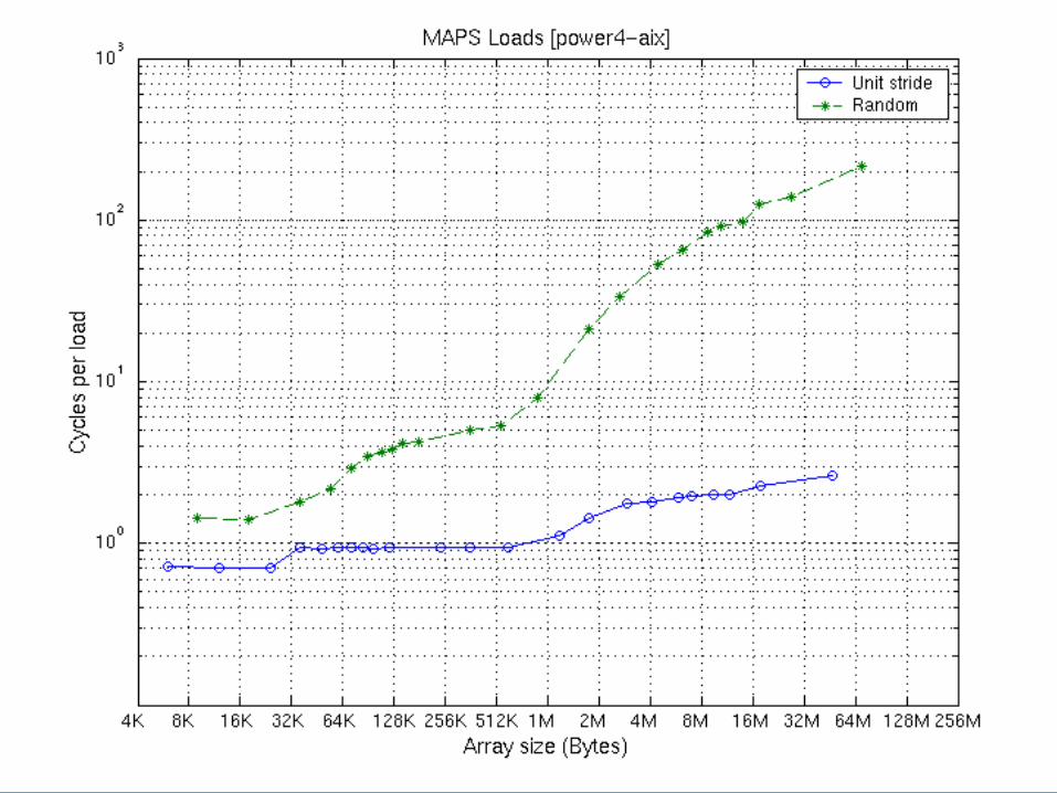
MAPS Benchmark Example: Power4

MAPS Benchmark Example: Itanium 2
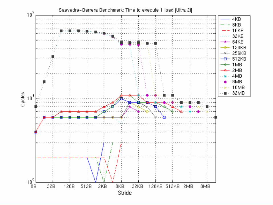
Saavedra-Barrera Example: Ultra 2i

Summary of Results: Pentium III
Summary of Results: Pentium III (3/3)

Execution Time Breakdown (PAPI): Matrix 40

Preliminary Results (Matrix Set 1): Itanium 2
LPFEM FEM (var) AssortedDense

Tuning Sparse Triangular Solve (SpTS)
• Compute x=L-1*b where L sparse lower triangular, x & b dense
• L from sparse LU has rich dense substructure– Dense trailing triangle can account for 20—90% of
matrix non-zeros
• SpTS optimizations– Split into sparse trapezoid and dense trailing triangle– Use tuned dense BLAS (DTRSV) on dense triangle– Use Sparsity register blocking on sparse part
• Tuning parameters– Size of dense trailing triangle– Register block size
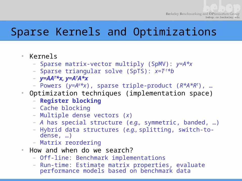
Sparse Kernels and Optimizations
• Kernels– Sparse matrix-vector multiply (SpMV): y=A*x– Sparse triangular solve (SpTS): x=T-1*b– y=AAT*x, y=ATA*x– Powers (y=Ak*x), sparse triple-product (R*A*RT), …
• Optimization techniques (implementation space)– Register blocking– Cache blocking– Multiple dense vectors (x)– A has special structure (e.g., symmetric, banded, …)– Hybrid data structures (e.g., splitting, switch-to-
dense, …)– Matrix reordering
• How and when do we search?– Off-line: Benchmark implementations– Run-time: Estimate matrix properties, evaluate
performance models based on benchmark data

Cache Blocked SpMV on LSI Matrix: Ultra 2i
A10k x 255k3.7M non-zeros
Baseline:16 Mflop/s
Best block size& performance:16k x 64k28 Mflop/s
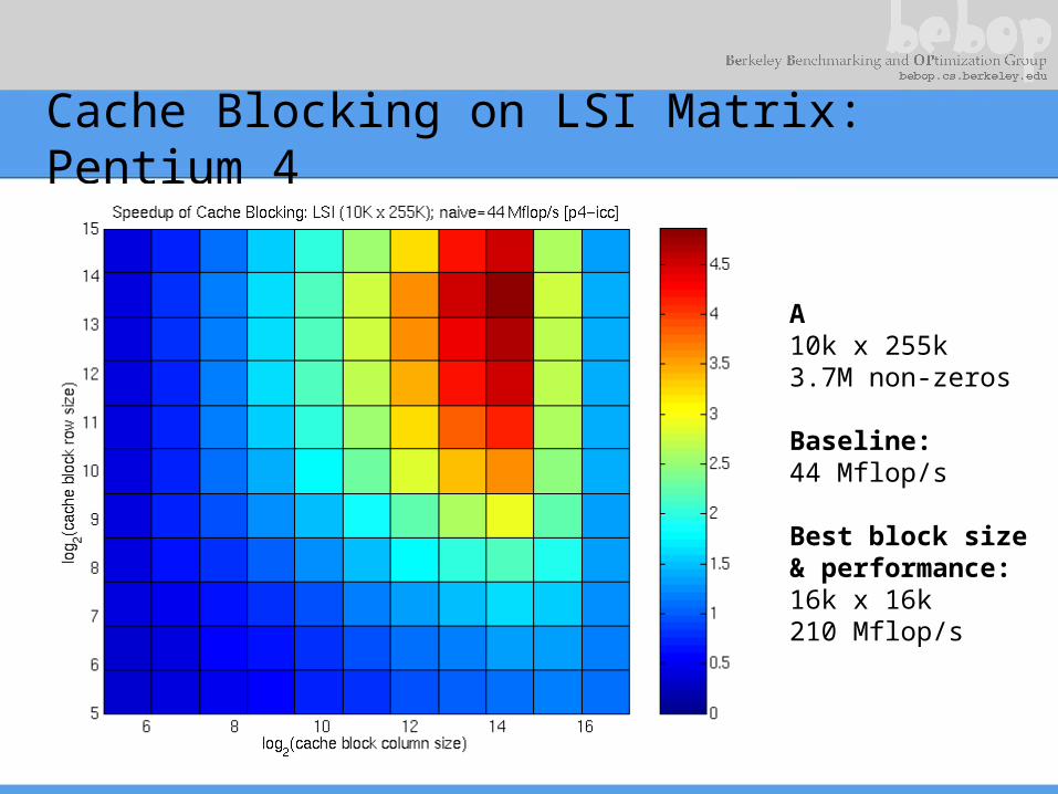
Cache Blocking on LSI Matrix: Pentium 4
A10k x 255k3.7M non-zeros
Baseline:44 Mflop/s
Best block size& performance:16k x 16k210 Mflop/s
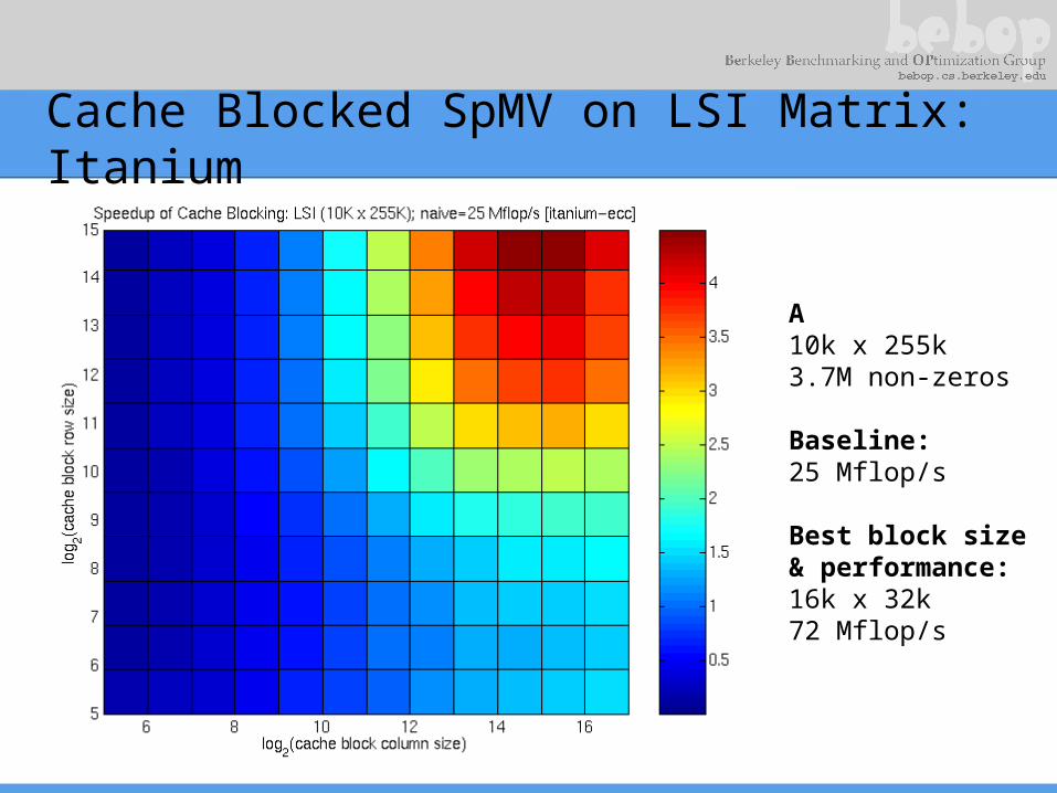
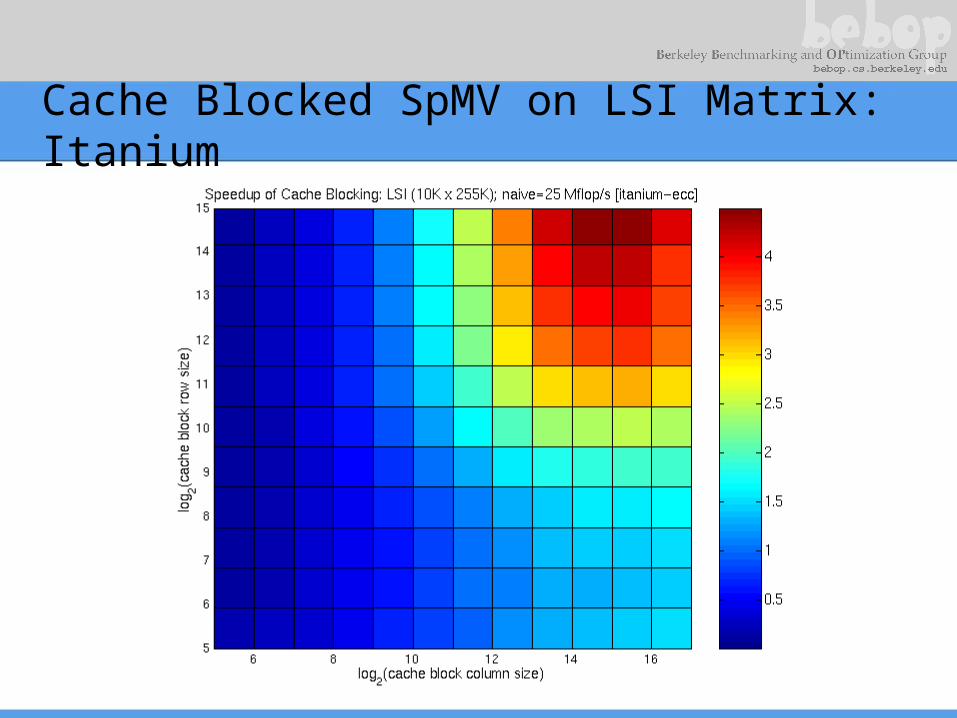
Cache Blocked SpMV on LSI Matrix: Itanium
A10k x 255k3.7M non-zeros
Baseline:25 Mflop/s
Best block size& performance:16k x 32k72 Mflop/s
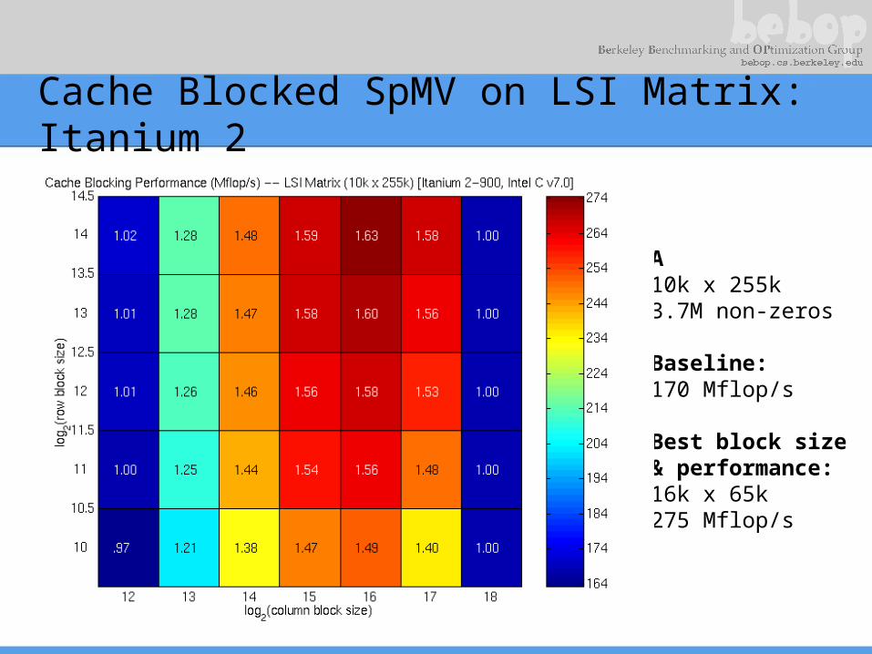
Cache Blocked SpMV on LSI Matrix: Itanium 2
A10k x 255k3.7M non-zeros
Baseline:170 Mflop/s
Best block size& performance:16k x 65k275 Mflop/s

Inter-Iteration Sparse Tiling (1/3)
• [Strout, et al., ‘01]• Let A be 6x6 tridiagonal• Consider y=A2x
– t=Ax, y=At
• Nodes: vector elements• Edges: matrix elements
aij
y1
y2
y3
y4
y5
t1
t2
t3
t4
t5
x1
x2
x3
x4
x5
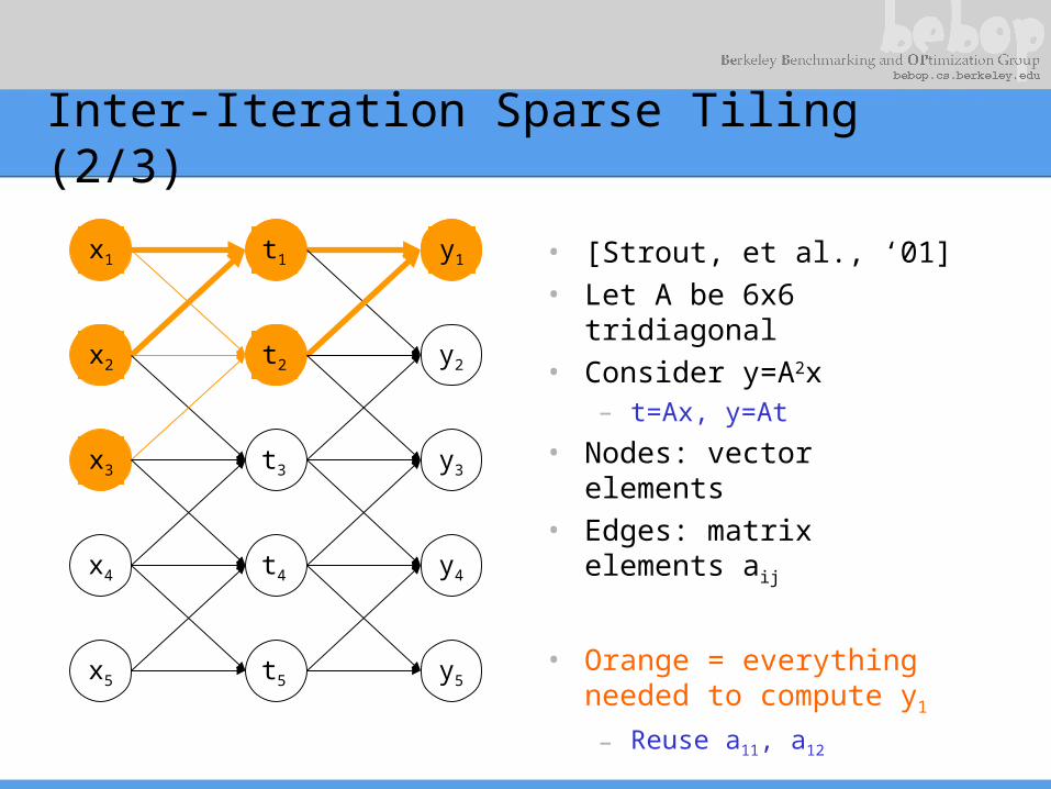
Inter-Iteration Sparse Tiling (2/3)
• [Strout, et al., ‘01]• Let A be 6x6 tridiagonal• Consider y=A2x
– t=Ax, y=At
• Nodes: vector elements• Edges: matrix elements
aij
• Orange = everything needed to compute y1
– Reuse a11, a12
y1
y2
y3
y4
y5
t1
t2
t3
t4
t5
x1
x2
x3
x4
x5
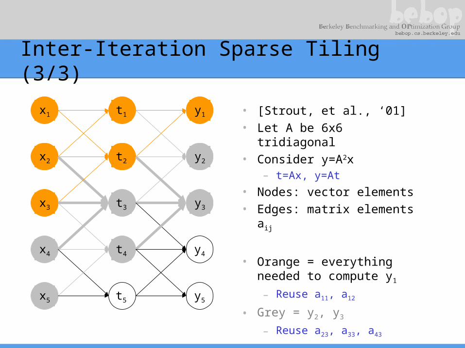
Inter-Iteration Sparse Tiling (3/3)
• [Strout, et al., ‘01]• Let A be 6x6 tridiagonal• Consider y=A2x
– t=Ax, y=At
• Nodes: vector elements• Edges: matrix elements
aij
• Orange = everything needed to compute y1
– Reuse a11, a12
• Grey = y2, y3
– Reuse a23, a33, a43
y1
y2
y3
y4
y5
t1
t2
t3
t4
t5
x1
x2
x3
x4
x5

Inter-Iteration Sparse Tiling: Issues
• Tile sizes (colored regions) grow with no. of iterations and increasing out-degree– G likely to have a few
nodes with high out-degree (e.g., Yahoo)
• Mathematical tricks to limit tile size?– Judicious dropping of
edges [Ng’01]
y1
y2
y3
y4
y5
t1
t2
t3
t4
t5
x1
x2
x3
x4
x5

Summary and Questions
• Need to understand matrix structure and machine– BeBOP: suite of techniques to deal with different sparse
structures and architectures• Google matrix problem
– Established techniques within an iteration– Ideas for inter-iteration optimizations– Mathematical structure of problem may help
• Questions– Structure of G?– What are the computational bottlenecks?– Enabling future computations?
• E.g., topic-sensitive PageRank multiple vector version [Haveliwala ’02]
– See www.cs.berkeley.edu/~richie/bebop/intel/google for more info, including more complete Itanium 2 results.

Exploiting Matrix Structure
• Symmetry (numerical or structural)– Reuse matrix entries– Can combine with register blocking, multiple vectors,
…
• Matrix splitting– Split the matrix, e.g., into r x c and 1 x 1– No fill overhead
• Large matrices with random structure– E.g., Latent Semantic Indexing (LSI) matrices– Technique: cache blocking
• Store matrix as 2i x 2j sparse submatrices• Effective when x vector is large• Currently, search to find fastest size
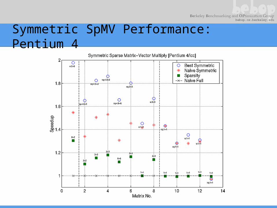
Symmetric SpMV Performance: Pentium 4

SpMV with Split Matrices: Ultra 2i
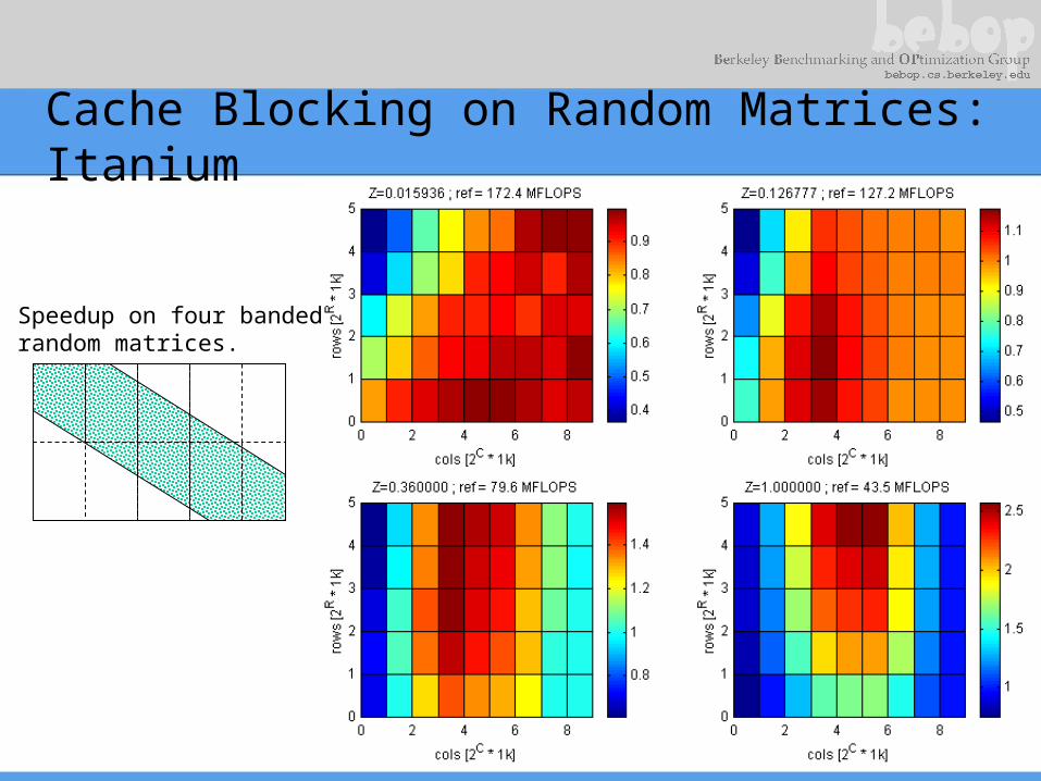
Cache Blocking on Random Matrices: Itanium
Speedup on four bandedrandom matrices.

Sparse Kernels and Optimizations
• Kernels– Sparse matrix-vector multiply (SpMV): y=A*x– Sparse triangular solve (SpTS): x=T-1*b– y=AAT*x, y=ATA*x– Powers (y=Ak*x), sparse triple-product (R*A*RT), …
• Optimization techniques (implementation space)– Register blocking– Cache blocking– Multiple dense vectors (x)– A has special structure (e.g., symmetric, banded, …)– Hybrid data structures (e.g., splitting, switch-to-dense, …)– Matrix reordering
• How and when do we search?– Off-line: Benchmark implementations– Run-time: Estimate matrix properties, evaluate
performance models based on benchmark data

Register Blocked SpMV: Pentium III
Register Blocked SpMV: Ultra 2i

Register Blocked SpMV: Power3

Register Blocked SpMV: Itanium

Possible Optimization Techniques
• Within an iteration, i.e., computing (G+uuT)*x once– Cache block G*x
• On linear programming matrices and matrices with random structure (e.g., LSI), 1.5—4x speedups
• Best block size is matrix and machine dependent
– Reordering and/or splitting of G to separate dense structure (rows, columns, blocks)
• Between iterations, e.g., (G+uuT)2x– (G+uuT)2x = G2x + (Gu)uTx + u(uTG)x + u(uTu)uTx
• Compute Gu, uTG, uTu once for all iterations• G2x: Inter-iteration tiling to read G only once

Multiple Vector Performance: Itanium

Sparse Kernels and Optimizations
• Kernels– Sparse matrix-vector multiply (SpMV): y=A*x– Sparse triangular solve (SpTS): x=T-1*b– y=AAT*x, y=ATA*x– Powers (y=Ak*x), sparse triple-product (R*A*RT), …
• Optimization techniques (implementation space)– Register blocking– Cache blocking– Multiple dense vectors (x)– A has special structure (e.g., symmetric, banded, …)– Hybrid data structures (e.g., splitting, switch-to-
dense, …)– Matrix reordering
• How and when do we search?– Off-line: Benchmark implementations– Run-time: Estimate matrix properties, evaluate
performance models based on benchmark data

SpTS Performance: Itanium
(See POHLL ’02 workshop paper, at ICS ’02.)
Sparse Kernels and Optimizations
• Kernels– Sparse matrix-vector multiply (SpMV): y=A*x– Sparse triangular solve (SpTS): x=T-1*b– y=AAT*x, y=ATA*x– Powers (y=Ak*x), sparse triple-product (R*A*RT), …
• Optimization techniques (implementation space)– Register blocking– Cache blocking– Multiple dense vectors (x)– A has special structure (e.g., symmetric, banded, …)– Hybrid data structures (e.g., splitting, switch-to-dense, …)– Matrix reordering
• How and when do we search?– Off-line: Benchmark implementations– Run-time: Estimate matrix properties, evaluate
performance models based on benchmark data
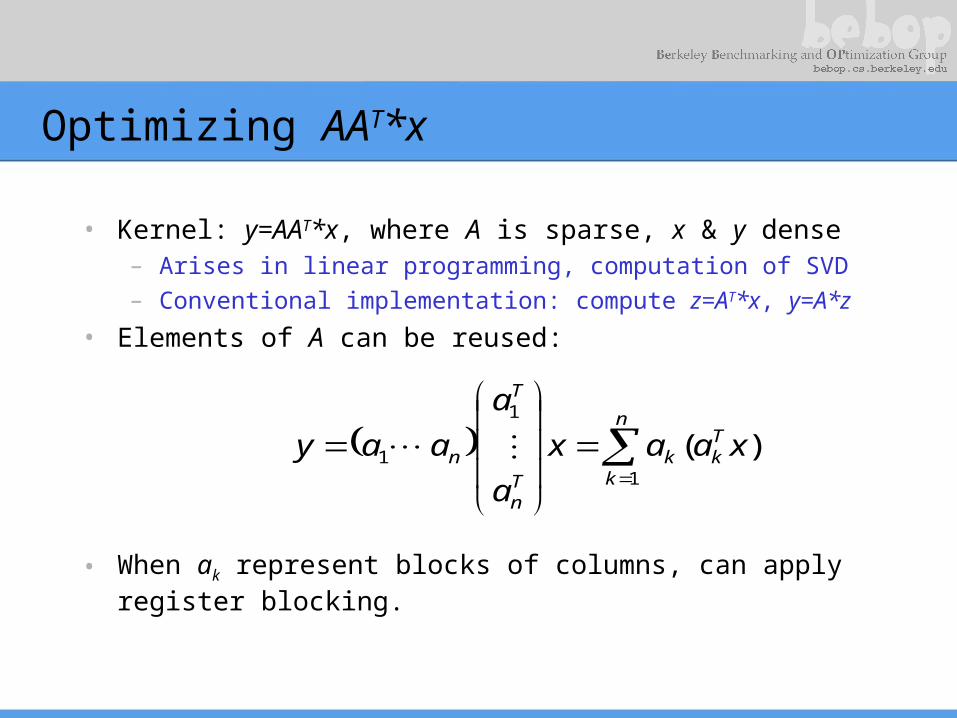
Optimizing AAT*x
• Kernel: y=AAT*x, where A is sparse, x & y dense– Arises in linear programming, computation of SVD– Conventional implementation: compute z=AT*x, y=A*z
• Elements of A can be reused:
n
k
Tkk
Tn
T
n xaax
a
a
aay1
1
1 )(
• When ak represent blocks of columns, can apply register blocking.

Optimized AAT*x Performance: Pentium III
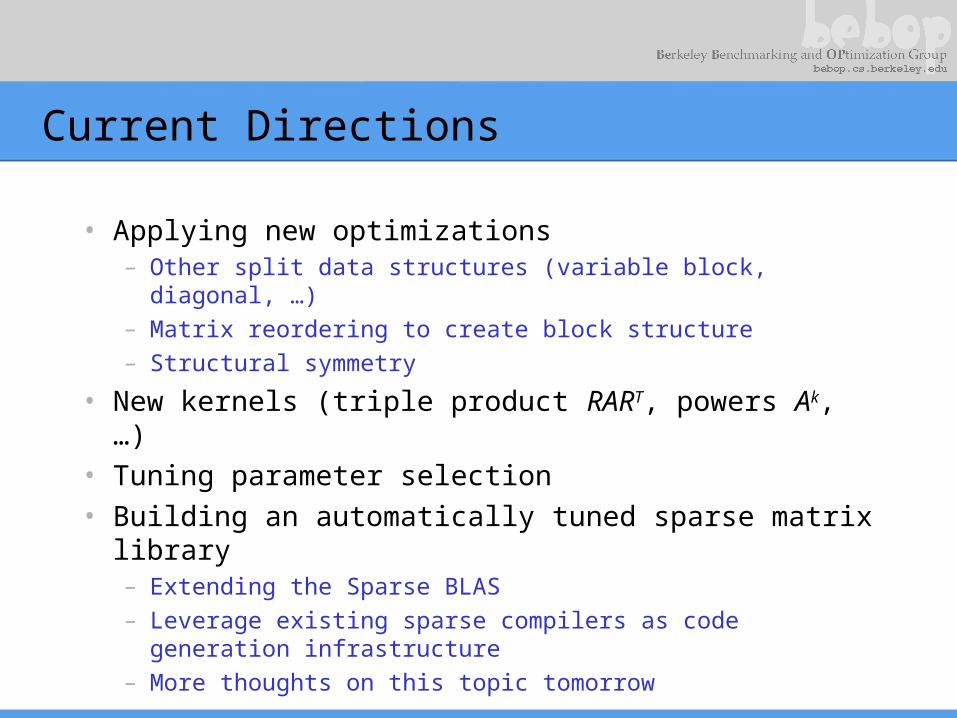
Current Directions
• Applying new optimizations– Other split data structures (variable block, diagonal,
…)– Matrix reordering to create block structure– Structural symmetry
• New kernels (triple product RART, powers Ak, …)• Tuning parameter selection• Building an automatically tuned sparse matrix
library– Extending the Sparse BLAS– Leverage existing sparse compilers as code
generation infrastructure– More thoughts on this topic tomorrow

Related Work
• Automatic performance tuning systems– PHiPAC [Bilmes, et al., ’97], ATLAS [Whaley & Dongarra
’98]– FFTW [Frigo & Johnson ’98], SPIRAL [Pueschel, et al.,
’00], UHFFT [Mirkovic and Johnsson ’00]– MPI collective operations [Vadhiyar & Dongarra ’01]
• Code generation– FLAME [Gunnels & van de Geijn, ’01]– Sparse compilers: [Bik ’99], Bernoulli [Pingali, et al., ’97]– Generic programming: Blitz++ [Veldhuizen ’98], MTL
[Siek & Lumsdaine ’98], GMCL [Czarnecki, et al. ’98], …
• Sparse performance modeling– [Temam & Jalby ’92], [White & Saddayappan ’97],
[Navarro, et al., ’96], [Heras, et al., ’99], [Fraguela, et al., ’99], …
More Related Work
• Compiler analysis, models– CROPS [Carter, Ferrante, et al.]; Serial sparse tiling
[Strout ’01]– TUNE [Chatterjee, et al.]– Iterative compilation [O’Boyle, et al., ’98]– Broadway compiler [Guyer & Lin, ’99]– [Brewer ’95], ADAPT [Voss ’00]
• Sparse BLAS interfaces– BLAST Forum (Chapter 3)– NIST Sparse BLAS [Remington & Pozo ’94];
SparseLib++– SPARSKIT [Saad ’94]– Parallel Sparse BLAS [Fillipone, et al. ’96]

Context: Creating High-Performance Libraries
• Application performance dominated by a few computational kernels
• Today: Kernels hand-tuned by vendor or user• Performance tuning challenges
– Performance is a complicated function of kernel, architecture, compiler, and workload
– Tedious and time-consuming
• Successful automated approaches– Dense linear algebra: ATLAS/PHiPAC– Signal processing: FFTW/SPIRAL/UHFFT
Cache Blocked SpMV on LSI Matrix: Itanium
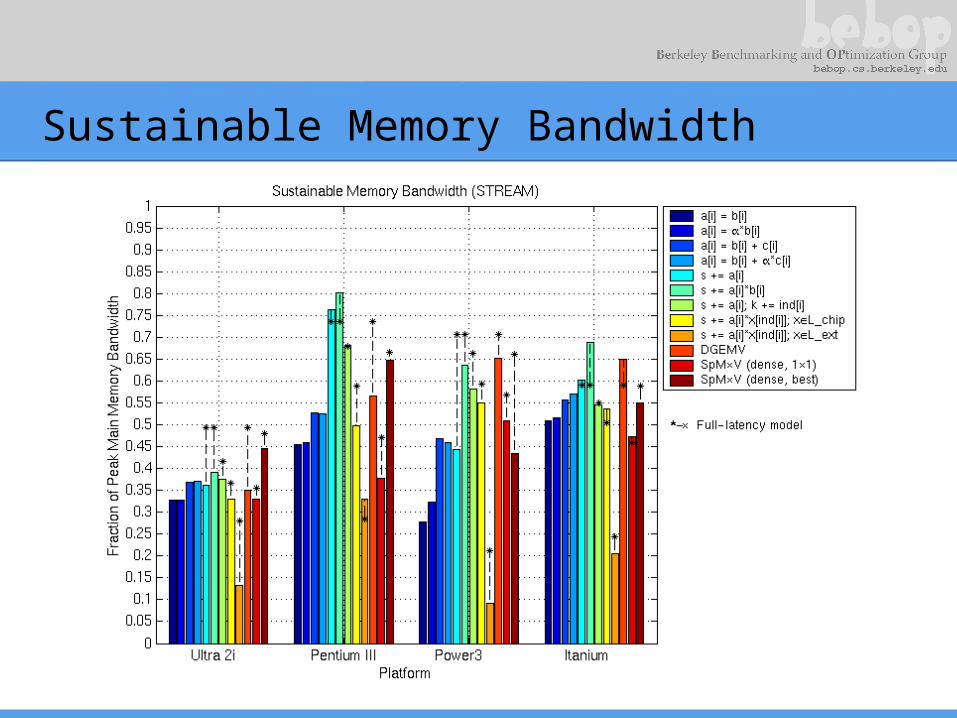
Sustainable Memory Bandwidth

Multiple Vector Performance: Pentium 4

Multiple Vector Performance: Itanium

Multiple Vector Performance: Pentium 4
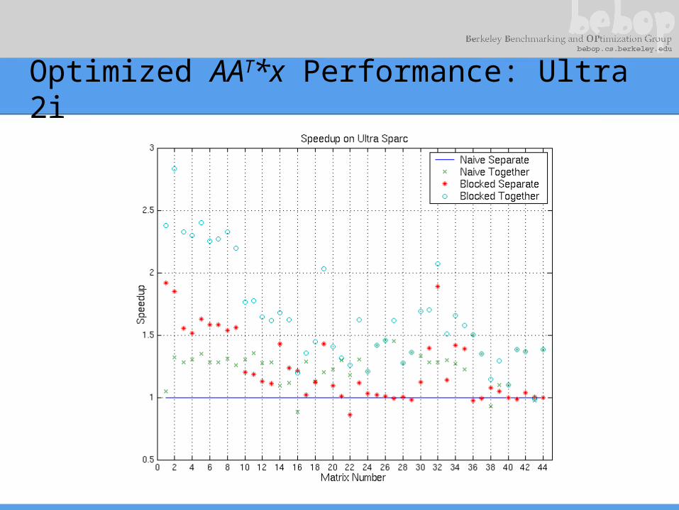
Optimized AAT*x Performance: Ultra 2i

Optimized AAT*x Performance: Pentium 4

Tuning Pays Off—PHiPAC
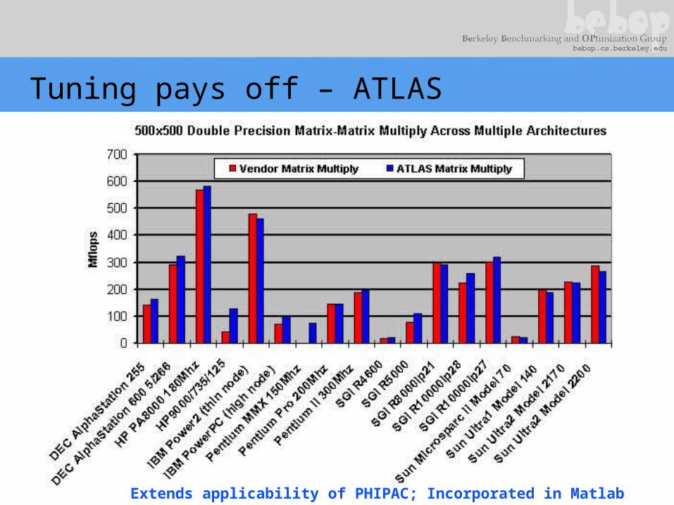
Tuning pays off – ATLAS
Extends applicability of PHIPAC; Incorporated in Matlab (with rest of LAPACK)

Register Tile Sizes (Dense Matrix Multiply)
333 MHz Sun Ultra 2i
2-D slice of 3-D space; implementations color-coded by performance in Mflop/s
16 registers, but 2-by-3 tile size fastest

High Precision GEMV (XBLAS)
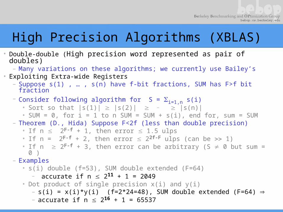
High Precision Algorithms (XBLAS)• Double-double (High precision word represented as pair of doubles)
– Many variations on these algorithms; we currently use Bailey’s• Exploiting Extra-wide Registers
– Suppose s(1) , … , s(n) have f-bit fractions, SUM has F>f bit fraction– Consider following algorithm for S = i=1,n s(i)
• Sort so that |s(1)| |s(2)| … |s(n)|• SUM = 0, for i = 1 to n SUM = SUM + s(i), end for, sum = SUM
– Theorem (D., Hida) Suppose F<2f (less than double precision)• If n 2F-f + 1, then error 1.5 ulps• If n = 2F-f + 2, then error 22f-F ulps (can be 1)• If n 2F-f + 3, then error can be arbitrary (S 0 but sum = 0 )
– Examples• s(i) double (f=53), SUM double extended (F=64)
– accurate if n 211 + 1 = 2049• Dot product of single precision x(i) and y(i)
– s(i) = x(i)*y(i) (f=2*24=48), SUM double extended (F=64) – accurate if n 216 + 1 = 65537

More Extra Slides
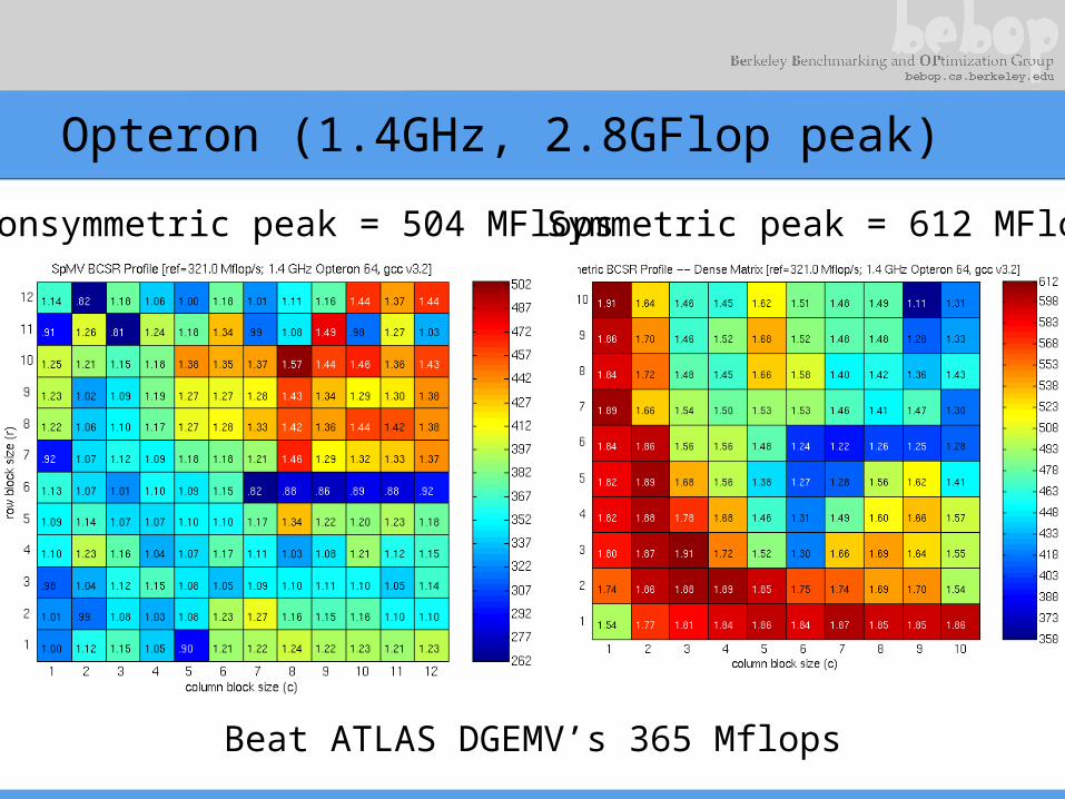
Opteron (1.4GHz, 2.8GFlop peak)
Beat ATLAS DGEMV’s 365 Mflops
Nonsymmetric peak = 504 MFlops Symmetric peak = 612 MFlops

Awards• Best Paper, Intern. Conf. Parallel Processing, 2004
– “Performance models for evaluation and automatic performance tuning of symmetric sparse matrix-vector multiply”
• Best Student Paper, Intern. Conf. Supercomputing, Workshop on Performance Optimization via High-Level Languages and Libraries, 2003– Best Student Presentation too, to Richard Vuduc– “Automatic performance tuning and analysis of sparse triangular solve”
• Finalist, Best Student Paper, Supercomputing 2002– To Richard Vuduc– “Performance Optimization and Bounds for Sparse Matrix-vector Multiply”
• Best Presentation Prize, MICRO-33: 3rd ACM Workshop on Feedback-Directed Dynamic Optimization, 2000– To Richard Vuduc– “Statistical Modeling of Feedback Data in an Automatic Tuning System”
Accuracy of the Tuning Heuristics (4/4)

Can Match DGEMV PerformanceDGEMV