automatic search of missing people in …amslaurea.unibo.it/15282/1/automatic...people_in... ·...
TRANSCRIPT

ALMA MATER STUDIORUM - UNIVERSITY OF BOLOGNA
SCHOOL OF ENGINEERING AND ARCHITECTURE
CASY Center for Research on Complex Automated Systems
DEI Department of Electrical, Electronic, and Information Engineering “Guglielmo Marconi”
MASTER DEGREE IN AUTOMATION ENGINEERING
GRADUATION THESIS
in
System Theory and Advanced Control
AUTOMATIC SEARCH OF MISSING PEOPLE IN
AVALANCHES
CANDIDATEFrancesco Ricciardi
SUPERVISOREminent Prof.
Lorenzo Marconi
CO-SUPERVISORDott. Nicola Mimmo
Academic Year 2016/2017
Graduation Session III


Abstract
One of the main source of danger for people practising activities in mountain en-
vironments is avalanches. In the early 70s has been commercialized the first model of
avalanche beacon transceiver: a device, composed by a transmitter and a receiver, spe-
cialized to the purpose of finding people buried under the snow. Since 2013, project
SHERPA is working to develop ground and aerial robots to support human in the search
of missing people in avalanches.
The aim of this dissertation is to provide a way to interface an avalanche beacon receiver
(ARTVA) with the autopilot module mounted on a quad-copter drone, and to study and
realize a software implementation of two automatic search algorithms, with the intention
of speeding up search operations with drones.
First we will focus on interfacing the ARTVA system with a quad-copter autopilot mod-
ule, named Pixhawk. This module embed a software, named PX4, which runs on a
real-time operating system (RTOS), and have several connection ports, among which
there is the serial one that we will use for our purpose. Then we will analyse how to use
the data coming from the ARTVA receiver to construct and implement the two search
algorithms. The idea is to generate set-points, based on the information coming from
the avalanche beacon receiver, and use them to feed the position controller which is
implemented in the PX4 firmware. Finally, we will execute simulations, provide results,
and investigate if a practical implementation is possible and what are the relative issues.
Le valanghe sono una delle principali fonti di pericolo per coloro che praticano attivita in
montagna. All’inizio degli anni ’70 e stato commercializzato il primo modello di apparec-
chio di ricerca travolti in valanga: si tratta di un dispositivo, composto da un trasmettitore
e un ricevitore, specializzato per la ricerca di persone seppellite nella neve. Fin dal 2013,
3

4 ABSTRACT
il progetto SHERPA sta lavorando allo sviluppo di un sistema di robot terrestri e aerei
con lo scopo di supportare l’uomo nella ricerca di dispersi in valanga.
L’obiettivo di questa trattazione e quello di trovare un modo per interfacciare il sistema
di ricerca dispersi in valanga con il modulo autopilota montato su un drone quadricot-
tero, e di studiare e realizzare una implementazione software di due algoritmi di ricerca
automatica, cosı da poter velocizzare le operazioni di ricerca con i droni.
In primis verra realizzato l’interfacciamento tra il sistema ARTVA e Pixhawk, un modulo
autopilota per quadricotteri. Il suddetto modulo incorpora un software, chiamato PX4,
che esegue su un sistema operativo in tempo reale, e inoltre dispone di diversi connet-
tori, tra cui la porta seriale che verra utilizzata al nostro scopo. Poi si indaghera come
utilizzare i dati ricevuti da ARTVA per costruire e utilizzare i due algoritmi di ricerca.
L’idea e quella di generare dei riferimenti, basandosi sui dati ottenuti dal ricevitore, e di
madmandarli al controllore di posizione gia implementato nel firmware di PX4. Infine,
verranno eseguite delle simulazioni, verranno mostrati i risultati, e si cerchera di capire
se e possibile una implementazione pratica e quali sono i relativi problemi.

Contents
Abstract 3
1 Introduction 15
1.1 Motivations . . . . . . . . . . . . . . . . . . . . . . . . . . . . . . . . . . 15
1.2 State of the art . . . . . . . . . . . . . . . . . . . . . . . . . . . . . . . . 16
2 ARTVA system and search algorithms 19
2.1 ARTVA system interfacing . . . . . . . . . . . . . . . . . . . . . . . . . . 19
2.1.1 ARTVA protocol data block . . . . . . . . . . . . . . . . . . . . . 21
2.1.2 Reading ARTVA data . . . . . . . . . . . . . . . . . . . . . . . . 23
2.1.3 Data validation algorithm . . . . . . . . . . . . . . . . . . . . . . 27
2.2 Flux Line search technique . . . . . . . . . . . . . . . . . . . . . . . . . . 29
2.2.1 Mathematical description . . . . . . . . . . . . . . . . . . . . . . 30
2.2.2 Implementation . . . . . . . . . . . . . . . . . . . . . . . . . . . . 33
2.3 Extremum Seeking search technique . . . . . . . . . . . . . . . . . . . . . 35
2.3.1 SISO scheme and linear analysis . . . . . . . . . . . . . . . . . . . 35
2.3.2 Non-local stability of non-linear case . . . . . . . . . . . . . . . . 38
2.3.3 Hybrid Extremum Seeking Control . . . . . . . . . . . . . . . . . 43
2.3.4 Implementation . . . . . . . . . . . . . . . . . . . . . . . . . . . . 47
2.4 General control scheme . . . . . . . . . . . . . . . . . . . . . . . . . . . . 49
3 Results 51
3.1 Simulations . . . . . . . . . . . . . . . . . . . . . . . . . . . . . . . . . . 51
3.1.1 Flux Line algorithm simulation . . . . . . . . . . . . . . . . . . . 53
3.1.2 HESC algorithm simulation . . . . . . . . . . . . . . . . . . . . . 56
5

6 ABSTRACT
3.1.3 Algorithms comparison . . . . . . . . . . . . . . . . . . . . . . . . 60
3.2 Practical implementation . . . . . . . . . . . . . . . . . . . . . . . . . . . 61
3.2.1 Test with motors off . . . . . . . . . . . . . . . . . . . . . . . . . 61
3.2.2 Test with motors on and no shielding . . . . . . . . . . . . . . . . 62
3.2.3 Test with motors on and standard aluminium shielding . . . . . . 63
3.2.4 Test with motors on and EMI aluminium shielding . . . . . . . . 64
Conclusions 65
A First Appendix 67
A.1 PX4 . . . . . . . . . . . . . . . . . . . . . . . . . . . . . . . . . . . . . . 67
A.1.1 Flight stack . . . . . . . . . . . . . . . . . . . . . . . . . . . . . . 67
A.1.2 Middleware . . . . . . . . . . . . . . . . . . . . . . . . . . . . . . 68
A.1.3 NuttX . . . . . . . . . . . . . . . . . . . . . . . . . . . . . . . . . 68
A.2 Communication over serial port . . . . . . . . . . . . . . . . . . . . . . . 68
A.2.1 Asynchronous serial protocol . . . . . . . . . . . . . . . . . . . . . 69
A.2.2 Rules of serial communication . . . . . . . . . . . . . . . . . . . . 70
A.3 Pubish/subscribe structure . . . . . . . . . . . . . . . . . . . . . . . . . . 71
A.3.1 Adding a new topic . . . . . . . . . . . . . . . . . . . . . . . . . . 72
A.3.2 Publish into a topic . . . . . . . . . . . . . . . . . . . . . . . . . . 72
A.3.3 Subscribe to a topic . . . . . . . . . . . . . . . . . . . . . . . . . . 73
A.4 ROS . . . . . . . . . . . . . . . . . . . . . . . . . . . . . . . . . . . . . . 74
A.4.1 Creating a package . . . . . . . . . . . . . . . . . . . . . . . . . . 74
A.4.2 Building the workspace and sourcing the setup file . . . . . . . . . 74
A.4.3 ROS nodes . . . . . . . . . . . . . . . . . . . . . . . . . . . . . . 75
A.4.4 ROS topics . . . . . . . . . . . . . . . . . . . . . . . . . . . . . . 75
A.4.5 Launch a ROS node with a launch file . . . . . . . . . . . . . . . 75
B Second Appendix 77
B.1 ARTVA system interfacing . . . . . . . . . . . . . . . . . . . . . . . . . . 77
B.1.1 Reading ARTVA data . . . . . . . . . . . . . . . . . . . . . . . . 77
B.1.2 Data validation algorith . . . . . . . . . . . . . . . . . . . . . . . 80

CONTENTS 7
B.2 Algorithms implementation . . . . . . . . . . . . . . . . . . . . . . . . . 84
B.2.1 Flux Line algorithm . . . . . . . . . . . . . . . . . . . . . . . . . 84
B.2.2 HESC algorithm . . . . . . . . . . . . . . . . . . . . . . . . . . . 86
Bibliography 89


List of Figures
1.1 Grid and Cross Flight algorithms operation . . . . . . . . . . . . . . . . 17
2.1 Magnetic dipole: moment and magnetic field . . . . . . . . . . . . . . . . 20
2.2 Data validation algorithm flowchart . . . . . . . . . . . . . . . . . . . . . 28
2.3 Flux Line search technique operation . . . . . . . . . . . . . . . . . . . . 30
2.4 Extremum Seeking Control scheme for a static map . . . . . . . . . . . . 35
2.5 Extremum Seeking Control scheme for plants with dynamics . . . . . . . 37
2.6 First order Extremum Seeking control scheme . . . . . . . . . . . . . . . 40
2.7 Higher order Extremum Seeking control scheme . . . . . . . . . . . . . . 42
2.8 General control scheme . . . . . . . . . . . . . . . . . . . . . . . . . . . . 50
3.1 Flux Line algorithm simulation case A . . . . . . . . . . . . . . . . . . . 54
3.2 Flux Line algorithm simulation case B . . . . . . . . . . . . . . . . . . . 54
3.3 Flux Line algorithm simulation case C . . . . . . . . . . . . . . . . . . . 55
3.4 Flux Line algorithm simulation case D . . . . . . . . . . . . . . . . . . . 55
3.5 Circle-shaped HESC algorithm simulation case A . . . . . . . . . . . . . 56
3.6 Circle-shaped HESC algorithm simulation case B . . . . . . . . . . . . . 57
3.7 Circle-shaped HESC algorithm simulation case C . . . . . . . . . . . . . 57
3.8 Circle-shaped HESC algorithm simulation case D . . . . . . . . . . . . . 58
3.9 Eight-shaped HESC algorithm simulation case A . . . . . . . . . . . . . . 58
3.10 Eight-shaped HESC algorithm simulation case B . . . . . . . . . . . . . . 59
3.11 Eight-shaped HESC algorithm simulation case C . . . . . . . . . . . . . . 59
3.12 Eight-shaped HESC algorithm simulation case D . . . . . . . . . . . . . . 60
A.1 Flight stack architecture . . . . . . . . . . . . . . . . . . . . . . . . . . . 68
9

10 LIST OF FIGURES
A.2 Example of parallel interface . . . . . . . . . . . . . . . . . . . . . . . . . 69
A.3 Example of serial interface . . . . . . . . . . . . . . . . . . . . . . . . . . 69
A.4 Example of a serial data frame . . . . . . . . . . . . . . . . . . . . . . . . 71

List of Tables
2.1 Protocol data block . . . . . . . . . . . . . . . . . . . . . . . . . . . . . . 22
3.1 Algorithms comparison . . . . . . . . . . . . . . . . . . . . . . . . . . . . 61
3.2 Test results: motors off . . . . . . . . . . . . . . . . . . . . . . . . . . . . 62
3.3 Test results: motors on, no shielding . . . . . . . . . . . . . . . . . . . . 63
3.4 Test results: motors on, simple aluminium shielding . . . . . . . . . . . . 63
3.5 Test results: motors on, EMI aluminium shielding . . . . . . . . . . . . . 64
11


List of Achronyms
SHERPA Smart collaboration between Humans and ground-aErial Robots
for imProving rescuing activities in Alpine environment
ARTVA Apparecchio di Ricerca Travolti in Valanga, search device of peo-
ple overwhelmed in avalanches
RTOS Real-Time Operating System
ICAR International Commission for Apline Rescue
GPS Global Positioning System
CRC Cyclic Redundancy Check
SISO Single-Input Single-Output
SPA Semi-global Practical Asymptotically
HESC Hybrid Extremum Seeking Control
FIFO First In First Out
ROS Robot Operating System
ESC Electronic Speed Controller
EMI Electromagnetic Interference
API Application Programming Interface
13

Chapter 1
Introduction
The goal of this project was to study, realize and simulate automatic search algorithms
with the aim of implementing them on a quad-copter drone by means of an autopilot
module. The aforesaid algorithms have the purpose to guide the drone toward people
buried under the snow in avalanches, so to minimize the time spent on the search, and
ensure a prompt intervention from rescuers. Those algorithms are generated using data
coming from an avalanche beacon system (ARTVA).
Since February 1st 2013 the European project SHERPA[1] is involved in the development
of a mixed ground and aerial robotics platform to support human in search and rescue
activities in unfriendly and hostile environments, like the alpine rescuing scenario, which
is specifically targeted by the project.
1.1 Motivations
A research made by the International Commission for Alpine Rescue (ICAR)[2] shows
that about 150 people are killed by avalanches every year in Europe and North America.
The overall survival rate of avalanche victims is 77%, and it mainly depends on the
grade and duration of burial. The analysis of a Swiss sample showed that 39% of people
involved in an avalanche were completely buried, and the survival probability in those
cases is 47.6%, versus 95.8% in cases of partial burial. These data highlight that grade
of burial is the strongest single factor for survival.
The above mentioned analysis shows also that survival probability remains above 80%
15
16 CHAPTER 1. INTRODUCTION
until 18 minutes after burial, a lapse of time referred as survival phase, falling thereafter
to 32%, in the so-called asphyxia phase. Another noticeable decrease in survival occurs
after 90 minutes, due to hypothermia combined with hypoxia and hypercapnia. There-
fore, also the duration of burial is very important and has to be taken in consideration.
Asphyxia was found to be the most common cause of death, and may occur in combi-
nation with trauma and hypothermia. So, the main recommendation is to locate and
extricate buried victims as quick possible.
The objective of SHERPA is to use quad-copters, which are not slowed by the hostility
of the terrain, to perform an automatic and rapid search of the victim, in such a way to
speed up the human intervention.
1.2 State of the art
As far as now, the efficiency of quad-copter drones supported by ARTVA systems in
rescuing operations has been tested with the implementation of a two phases search al-
gorithm, while a terrain following one is in charge of making the vehicle maintain always
a certain altitude from the ground.
After take-off, the quad-copter reaches a defined altitude and starts the Grid Flight[3]
phase, during which it follows previously defined length parallel lines, placed at a certain
distance from each other. More precisely, the drone travels a line until its end, then it
move toward the next line following a trajectory perpendicular to the lines, and, once
reached the next line, it travels that line backward until the end, keeping on describing
a sort of grid-shaped path until the first signal coming from the beacon is acquired.
At this point, the Cross Flight phase starts, making the quad-copter perform the follow-
ing operations:
• Forward flight until the beacon signal is lost, storing the GPS position when it
happens; then, the flight segment continues to ensure avoiding false null signal
detection and, in the case, the GPS position is updated.
• Backward flight until the beacon signal is found again and continue flying until it
is lost, storing so the second GPS point.

1.2. STATE OF THE ART 17
• The autopilot module computes the midpoint between the two GPS acquired lo-
cation and lead the drone to it.
• Turn 90 and repeat the forward and backward flight in order to identify the next
two GPS points, namely the other two vertices of the cross.
• The autopilot module computes the midpoint between the two GPS acquired lo-
cation and flies the quad-copter to it.
This point should be the one with the highest signal strength corresponding to the
position of the transmitting beacon. The operation of this algorithm is shown in Figure
1.1. This search algorithm has been found to perform well, especially when wide areas
need to be surveyed. However, our purpose is to improve search times by replacing the
Cross Flight phase with an algorithm that is capable of drive the vehicle directly to the
position of the beacon transmitter.
Figure 1.1. Grid and Cross Flight algorithms operation: the blue arrows represent Grid Flight,
the green arrows represent Cross Flight, the red cross represents the transmitter’s position.


Chapter 2
ARTVA system and search
algorithms
Now we will analyse first the ARTVA beacon system and how to interface it to
Pixhawk autopilot module, and so to read and handle the data coming from the ARTVA
receiver with PX4 software running on the aforementioned module. Then we will study
two possible search algorithms and how to implement them. The description of PX4
software and some of its basic concept are reported in the first appendix, while all the
code used to realize the interfacing between the beacon receiver and the autopilot module,
the reading of data, and the implementation of the search algorithms, is reported in the
second appendix.
2.1 ARTVA system interfacing
The avalanche beacon system (ARTVA) used in our application includes a transmitter
and a receiver which can be mounted on the quad-copter drone and activated during the
search of missing people. Typical features of beacon transmitters are:
• carrier frequency of 457 kHz,
• up to 200 hours battery life,
• search range of about 50 metres.
19

20 CHAPTER 2. ARTVA SYSTEM AND SEARCH ALGORITHMS
ARTVA transmitter’s flux lines behave as the external magnetic field produced by the
magnetic dipole moment, represented in Figure 2.1; they propagates from a pole to
the opposite one, following an ellipse fashion with growing amplitude. Conversely, the
ARTVA receiver transform the signal received from the transmitter in two values:
Distance (d) Represents receiver’s distance from the transmitter and it is computed as
the inverse of signal’s intensity.
Angle (δ) It is the angle between the direction of the receiver and the line tangent to
the flux ellipse to which the receiver is located.
Figure 2.1. Magnetic dipole: the blue thick arrow represents the moment, the black thin
arrows represent the magnetic field.
It is possible to identify three operation zones, depending on the distance between the
transmitter and the receiver:
Outer zone The transmitter is too far from the receiver, the received distance value d
is equal to −1 or to the designed maximum value, depending on the model of the
receiver, while the received angle value δ is equal to zero.
Mid zone The receiver distance value d is in the range between 250 and the designed
maximum value, while the received angle value δ can vary between −90 and +90,

2.1. ARTVA SYSTEM INTERFACING 21
which are intended to be degrees, depending on the orientation of the receiver with
respect to the transmitter.
Inner zone The transmitter is close to the receiver (in a radius of about 3 metres), the
received distance value d is lower or equal to 300, while the received angle value δ
is equal to zero.
The middle and the inner zones are the useful ones, providing information about the
transmitter’s position, while we cannot conclude anything with the data obtained in the
outer zone, except that we are too far from the target.
2.1.1 ARTVA protocol data block
The message sent from the ARTVA receiver to Pixhawk autopilot module is a 32
byte length data block, with 8-N-1 data format, sent with a baud rate of 9600 bps. The
frequency of transmission is 5 Hz, so a new message is sent each 200 ms. Moreover, the
number format of the message is little-endian.
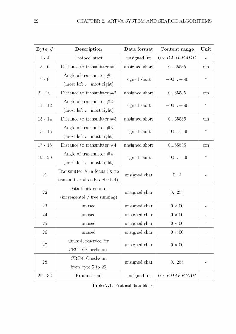
The structure of the data block is presented in Table 2.1: as we can see, the first 4 bytes
are reserved for the protocol header, bytes from 5 to 20 contains the useful data, byte
21 indicates the number of transmitter which is in focus, while byte 22 is an incremental
counter. Then there are a bunch of bytes, from 23 to 27, which are unused, followed by a
single byte which is used for the CRC-8 checksum. Finally, the last 4 bytes are reserved
for the protocol footer.
Protocol’s header and footer As said before, both the protocol’s header and footer
are 4 bytes length, and, as the names suggest, they are placed at the start and at
the end of the data block, respectively. They are used in the validity check phase
to distinguish between correct messages and broken ones. Both of them are a fixed
hexadecimal number, 0×BABEFADE for the header and 0×EDAFEBAB for
the footer, both expressed in little-endian number format.
Useful data The useful data of the messages are represented by 4 distances and 4
angles. The distance and angle values that we need depend on the number of
transmitter in focus, e.g. if transmitter in focus is the number 1, we need to
22 CHAPTER 2. ARTVA SYSTEM AND SEARCH ALGORITHMS
Byte # Description Data format Content range Unit
1 - 4 Protocol start unsigned int 0×BABEFADE -
5 - 6 Distance to transmitter #1 unsigned short 0...65535 cm
7 - 8Angle of transmitter #1
(most left ... most right)signed short −90...+ 90
9 - 10 Distance to transmitter #2 unsigned short 0...65535 cm
11 - 12Angle of transmitter #2
(most left ... most right)signed short −90...+ 90
13 - 14 Distance to transmitter #3 unsigned short 0...65535 cm
15 - 16Angle of transmitter #3
(most left ... most right)signed short −90...+ 90
17 - 18 Distance to transmitter #4 unsigned short 0...65535 cm
19 - 20Angle of transmitter #4
(most left ... most right)signed short −90...+ 90
21Transmitter # in focus (0: no
transmitter already detected)unsigned char 0...4 -
22Data block counter
(incremental / free running)unsigned char 0...255 -
23 unused unsigned char 0× 00 -
24 unused unsigned char 0× 00 -
25 unused unsigned char 0× 00 -
26 unused unsigned char 0× 00 -
27unused, reserved for
CRC-16 Checksumunsigned char 0× 00 -
28CRC-8 Checksum
from byte 5 to 26unsigned char 0...255 -
29 - 32 Protocol end unsigned int 0× EDAFEBAB -
Table 2.1. Protocol data block.

2.1. ARTVA SYSTEM INTERFACING 23
acquire values from distance 1 and angle 1. The distance to transmitter value is a
2 bytes unsigned integer number in the range between 0 and 65535, and represents
a distance in centimetres; the angle of transmitter value is a 2 bytes signed integer
number in the range between −90 and +90, and represents an angle in degrees.
Each byte contains an hexadecimal number and, as said before, all values are
expressed in little-endian number format, so we will need to use the techniques of
masking and bit-shifting to reconstruct the values in such a way we can use them
as decimal numbers.
Scrambler Another thing to take into account is that the data block is scrambled by
adding the hexadecimal number 0 × 55 to each byte, in such a way to avoid long
sequences of 0 and 1. Thus, for descrambling data, we have to subtract 0×55 from
each byte.
CRC-8 checksum The checksum is used to verify data integrity, detecting error that
may be introduced during the transmission. The CRC-8 checksum is a single byte
unsigned character, which can assume integer values between 0 and 255, generated
based on generator polynomial g(x) = x8 + x2 + x+ 1.
2.1.2 Reading ARTVA data
The procedure used to read the data sent through the serial port by the ARTVA
receiver is implemented in a Pixhawk module named artva, and is composed of the
following steps:
• setting up and opening of the serial port (autopilot module side);
• read the arriving message;
• check the validity of the message;
• parse the message.
After these steps are correctly executed, the decoded message is ready to be published
in the apposite topic. Basic concepts of communication over a serial port are reported
in the first appendix. Now we will analyse each step of the reading procedure.

24 CHAPTER 2. ARTVA SYSTEM AND SEARCH ALGORITHMS
Setup and open serial port
In this step, we first set up the port by specifying the uart name of the serial port
to be opened, in our case /dev/ttyS6 (which corresponds to the serial 4 port of the
Pixhawk), and the data format, which, as previously said, is 8-N-1 9600 bps baud rate.
Then we can open the serial port by associating a file descriptor fd to the open() function
as follows:
fd = open(port, O_RDONLY | O_NOCTTY | O_NDELAY);
Where port is the name of the serial port, and the other three terms in the second field
of the function are flags. If the file descriptor fd returns a value equal or lower than 0,
it means that the connection to the port is failed; otherwise, the setting up and opening
procedure is finished and we can go on reading the message.
Read the message
The read() function can read from a serial port only one byte for each call so, if we
want to read a packet of bytes, we have to perform a call of the read() function for each
byte. This means that in our case, in which we want to read a 32 byte data block, we
have to realize a read cycle by means of a while() loop, so to execute a single read() for
each byte. The reading algorithm is executed by calling the following function:
int read_port()
The while() loop does not start until the procedure reads a byte containing the hexadec-
imal number 0×DE, which is the first byte of the message’s header. This is a precaution
needed to avoid the corruption of the data. In fact, it may happen that one or more
bytes are skipped for any reason. If this happens, performing the read procedure by just
using the while() loop will result in having a message buffer in which the header, the
content and the footer are not in the right places, because each byte in the buffer has
been shifted from its original position. This will lead to read all non-valid message, since
now the first 4 bytes of the buffer do not contain the right values of the header (and the
same is for the last 4 bytes which does not match the footer), and it will be the same for
all the successive reading cycles.

2.1. ARTVA SYSTEM INTERFACING 25
By performing the read of the first byte out of the cycle, we can ensure that, even if there
is a lose of some bytes, the reading cycle does not start until the algorithm recognizes
the header’s first byte, and so the positions of the next message’s bytes are not shifted.
Moreover, the buffer is cleaned at each new message read procedure, and the data are
descrambled by subtracting the hexadecimal number 0× 55 to each byte.
Validity check
The check of the message validity is performed by just ensuring that the values of the
first 4 bytes and of the last 4 ones are equal to the values of the header and the footer.
To run the validity check algorithm, we have to call the following function:
int check_ARTVA()
If a message does not pass the validity check, it is discarded and the algorithm wait for
the next message.
Message parsing
This part of the reading procedure has the purpose of reorder the bytes which consti-
tute the useful part of the message, namely distances and angles values, so to transform
the number format from little-endian to big-endian. The techniques of masking and
bit-shifting, used for this transformation, can be summarized in the following steps:
• take the 2 bytes we want to transform (e.g. 00000010 00101001 in binary) and take,
as a mask, the hexadecimal number 0 × FF00, which corresponds to the binary
number 11111111 00000000, then perform an AND operation:
0000010 00101001 AND 11111111 00000000 = 00000010 0000000
• Shifting the first of the 2 so obtained bytes to the right 8 places, we have basically
found the first byte:
00000000 0000010

26 CHAPTER 2. ARTVA SYSTEM AND SEARCH ALGORITHMS
• Repeating now the same AND operation, but taking a slightly different mask,
namely the hexadecimal number 0 × 00FF , corresponding to the binary number
00000000 11111111:
00000010 00101001 AND 00000000 11111111 = 0000000 00101001
• Shifting these 2 bytes to the left 8 places by using the << 8 operator, we found
the second byte:
00101001 00000000
• Finally, summing up the 2 obtained bytes, we found the 2 bytes reordered in big-
endian number format:
00101001 00000010
To execute the message parsing, this function must be called:
int parse_ARTVA()
By means of the masking and bit-shifting techniques applied on the message sent by the
ARTVA receiver, we are able to reconstruct the distances and the angles values expressed
in decimal numbers.
Publishing data
When the reading procedure is complete and the message has been correctly decoded,
the values of distances and angles, the value representing the transmitter in focus, and
the value of the data block counter are published into a topic named artva data so that
they can be recalled and used in real-time by the Pixhawk module which performs the
ARTVA data validation and the set-point generation. The string of code used to publish
the data is the following:
orb_publish(ORB_ID(artva_data), artva_topic_pub, &sens);
The publish/subscribe structure and how to use it is described in the first appendix.

2.1. ARTVA SYSTEM INTERFACING 27
2.1.3 Data validation algorithm
Once a new ARTVA measure has been read, we need to check if it is a valid one, so to
discard all eventual wrong values coming from disturbances and electromagnetic noises.
In order to check the validity of a measure, we have to check if it is consistent with
the last values found, namely if it does not differ too much from them. To perform this
data validation, the PX4 module set point, which is in charge of computing the set-point
values (position or velocity, depending on the algorithm in use) to feed the controller,
contains also a two-phase validation procedure.
The first thing to do is subscribe to the topic containing the data we need: the topic
containing the data read from ARTVA, and the one containing the vehicle position, since
we will later need to know the yaw angle of the quad-copter. We can subscribe to those
topics by means of the following strings of code:
orb_check(artva_topic_sub, &updated);
if (updated) orb_copy(ORB_ID(artva_data), artva_topic_sub, &sensor);
orb_check(yaw_topic_sub, &updated);
if (updated) orb_copy(ORB_ID(vehicle_local_position), yaw_topic_sub, &pos);
The set point module runs first a parse algorithm to determine which of the four pairs
of values (distances and angles) are the interesting ones, then executes the following two
functions:
• first validation,
• step validation,
which together constitute the data validation algorithm. A flowchart of the algorithm is
shown in Figure 2.2.
Parsing data
The parsing function decides which distance and angle values to take in consideration
by just selecting the distance value which is below the admissible threshold, imposted to
2500 (about 25 metres), and its relative angle value. If there are no distances values below
the threshold, the function says that no transmitter has been detected. This function

28 CHAPTER 2. ARTVA SYSTEM AND SEARCH ALGORITHMS
Figure 2.2. Data validation algorithm flowchart.
also imposes the validity ranges for distances and angles to be used in the validation
procedure. Parsing of data is performed by calling the following function:
int parse_data()
First validation
The first validation procedure aims to find fk consecutive consistent values, where
fk is a tunable coefficient, checking consistency of both distances and angles. If it suc-
ceeds, the algorithm proceeds to the next validation phase; otherwise, if a non consistent
2.1. ARTVA SYSTEM INTERFACING 29
values is found before collecting fk consecutive consistent values, the procedure restarts.
Consistency of the values is checked by using the validity ranges defined in the parsing
function:
if current value ∈ (last value∓ validity range)
then current value is valid
Angles values are considered in modulus, since there are points in which they can change
from −90 to +90. Once fk consecutive consistent values are found, and the algorithm
can move to the next phase, the last arrived values are used as sample values for the
next validation procedure. To execute the first validation algorithm we have to call the
following function:
int first_validation()
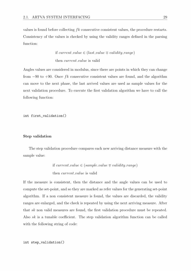
Step validation
The step validation procedure compares each new arriving distance measure with the
sample value:
if current value ∈ (sample value∓ validity range)
then current value is valid
If the measure is consistent, then the distance and the angle values can be used to
compute the set-point, and so they are marked as refer values for the generating set-point
algorithm. If a non consistent measure is found, the values are discarded, the validity
ranges are enlarged, and the check is repeated by using the next arriving measure. After
that sk non valid measures are found, the first validation procedure must be repeated.
Also sk is a tunable coefficient. The step validation algorithm function can be called
with the following string of code:
int step_validation()

30 CHAPTER 2. ARTVA SYSTEM AND SEARCH ALGORITHMS
2.2 Flux Line search technique
The first algorithm we are going to present is based on the fact that the ARTVA
transmitter behave like a magnetic dipole. The main idea is to exploit this characteristic
to align the drone to a flux line, and make the vehicle follow it until it reaches the beacon
transmitter. Practically speaking, at each new ARTVA data received, we want the drone
to compensate its yaw inclination with respect to the line tangent to the flux ellipse, and
to move along that direction, as it is shown in Figure 2.3. The output of the algorithm
will be a velocity set-point (and also a yaw correction).
Figure 2.3. Flux Line search technique operation: the red arrow represents the velocity
set-point, the light blue arrows represents the yaw correction.
2.2.1 Mathematical description
The drone is guided toward the victim by means of the following reference velocity[4]:
v∗(τ) = vδ(k)vmaxKd(k)√
1 +K2d2(2.1)

2.2. FLUX LINE SEARCH TECHNIQUE 31
valid ∀τ ∈ [k, k + ∆T ], where
vδ =
cos δ(k)
sin δ(k)
0
Moreover, K is a tunable coefficient, while vmax represents the drone’s maximum speed
in the horizontal plane. The yaw reference, designed to make the X-axis of the drone’s
reference frame aligned with the direction of v∗(τ), is computed by means of the following
law:
ψ∗(τ) = ψ(k) + δ(k) (2.2)
valid ∀τ ∈ [k, k + ∆T ]
Stability analysis
For the purpose of analysing the stability of the search based on flux lines, we can
represent the transmitter’s nominal magnetic field as follows:
H =1
4πr5Am (2.3)
where
A =
2x2 − y2 − z2 3xy 3xz
3xy 2y2 − x2 − z2 3yz
3xz 3yz 2z2 − x2 − y2
and r2 = x2 + y2 + z2 is the actual Cartesian distance from the transmitter to the
receiver, and m = [mx my mz]T represents the transmitter magnetic moment, in the
inertial reference frame. Furthermore, to reduce the calculus complexity, we can centre,
without loss of generality, the inertial frame Fi on the transmitter, which is generically
oriented on the inertial xi-zi plane. Given Hxiyi = [Hxi Hyi ]T , projection of H on the
inertial xi-zi plane, the following analysis is conducted by imposing the X-axis of the
drone’s reference frame aligned with the Hxiyi vector, the Z-axis of the drone’s reference

32 CHAPTER 2. ARTVA SYSTEM AND SEARCH ALGORITHMS
frame parallel to the inertial zi-axis, and the Y -axis of the drone’s reference frame aligned
consequently. Finally, the centre O of the drone’s reference frame is placed on the inertial
xi-yi plane at the coordinates identified by means of the couple (x, y). Given the time
instant k, it is possible to introduce a polar coordinate change:x(k)
y(k)
=
ρ(k) cos θ(k)
ρ(k) sin θ(k)
(2.4)
Then, the vector Hxiyi can be described in terms of its parallel and perpendicular com-
ponents with respect to the radius ρ(k):H‖H⊥
=
cos θ(k) sin θ(k)
− sin θ(k) cos θ(k)
Hxi
Hyi
(2.5)
Assuming that the inertial drone’s reference velocity v∗i (k) is taken along the direction
of the vector Hxiyi with modulus ||v∗(k)|| > 0, we have that:v∗ix(k)
v∗iy(k)
=||v∗(k)||||Hxiyi ||
Hxi
Hyi
(2.6)
which can also be expressed in terms of parallel and perpendicular components with
respect to the radius ρ(k): v∗i‖
(k)
v∗i⊥(k)
=||v∗(k)||||Hxiyi ||
H‖H⊥
(2.7)
The angle θ(k) can be changed if and only if the perpendicular component of the velocity
is different from zero.
ρθ(k) = v∗i⊥(k) =||v∗(k)||||Hxiyi ||
mxρ2(k) · sin θ(k) (2.8)
Proposition 1 For any initial condition (ρ(0), θ(0)) with ρ(0) > 0 and θ(0) 6= 0, the

2.2. FLUX LINE SEARCH TECHNIQUE 33
tracking of the references (2.1) and (2.2) guarantees that
limk→∞
θ(k) = π
Proposition 2 For any initial condition (ρ(0), θ(0)) with ρ(0) > 0 and π2< θ(0) < 3π
2,
the tracking of the references (2.1) and (2.2) guarantees that
limk→∞
ρ(k) = 0
Remark The composition of Proposition 1 and Proposition 2 says that if the search
starts with initial conditions given by ρ > 0 and θ ∈ (−π2, π
2), the radius increases
until the angle θ does not reach the compact domain [π2, 3π
2]. This problem is solved
with the direction inversion procedure later described.
2.2.2 Implementation
The Flux Line set-point generation algorithm follows the steps below:
Direction check Once every ck data received, where ck is a tunable coefficient, stores
a distance value. Each time new data pass the validation algorithm, compares
the distance value of the new data with the last stored one. If the new value is
greater than the stored one, changes sign to the formula that computes the set-
point. Moreover, only for the current iteration, instead of computing a new velocity
set-point, the algorithm will publish the last computed set-point changed in sign.
In this way the drone will come back to the previous position before the algorithm
starts computing new set-point values in the opposite direction.
Yaw correction Computes the yaw correction to be applied to the drone if the angle
values received from ARTVA is greater than a certain threshold:
if angle value > threshold then apply the yaw correction
The yaw correction is saturated to a maximum value in such a way to be applied

34 CHAPTER 2. ARTVA SYSTEM AND SEARCH ALGORITHMS
gradually each time a new set-point is given to the controller:
if angle value ≤ yaw correction max then yaw correction = angle value
else yaw correction = yaw correction max
In this way, we avoid to have non-consistent consecutive ARTVA measures, which
will create difficulties in the data validation phase.
Velocity set-point computation Uses the current distance value to compute the ve-
locity set-point, so that the closer the drone is to the beacon transmitter, the lower
is the imposed velocity. Also the generated velocity is saturated to a maximum
value:
if distance value ≤ velocity max then velocity set point = distance value
else velocity set point = velocity max
In order to be passed to the controller, the velocity set-point value, which is in-
tended in the direction tangent to the flux ellipse, must be decomposed along the
X and Y directions of the drone body frame:
vspx = sign · vsat · cos(δ)
vspy = sign · vsat · sin(δ)(2.9)
where δ, which is the angle value received from ARTVA, is equal to zero if the yaw
angle has been completely compensated.
Reference system transformation Transforms the reference system from the one in
agreement with the body to the inertial one:
vspX = vspx · cos(γ) + vspy · sin(γ)
vspY = −vspx · sin(γ) + vspy · cos(γ)(2.10)
where γ is the residual value of the yaw angle of the drone after the correction.
Finally, the algorithm publishes the two values of the velocity set-point and the value of
yaw correction to a topic from which the controller can read them.

2.3. EXTREMUM SEEKING SEARCH TECHNIQUE 35
2.3 Extremum Seeking search technique
The next presented algorithm is based on the Extremum Seeking Control, a control
technique which aim to select the set-point to keep the output at the extremum value
(maximum or minimum). In our case, we want to use this kind of control to search for
the minimum value of the distance from the beacon transmitter.
2.3.1 SISO scheme and linear analysis
Extremum Seeking for a static map
Figure 2.4. Extremum Seeking Control scheme for a static map.
Considering the Extremum Seeking scheme for a static map[5], represented in Figure
2.4, we have that:
f(ϑ) = f ∗ +f ′′
2(ϑ− ϑ∗)2 (2.11)
where f ′′ > 0. If f ′′ < 0, replace k (k > 0) with −k, so to obtain f ′′ > 0. The purpose is
to make ϑ−ϑ∗ as small as possible, so that the output y = f(ϑ) is driven to its minimum.
The perturbation signal a ·sin(ωt) helps to get a measure of gradient information of f(ϑ).
Defining the following quantities:
• ϑ∗: optimal input (unknown);
• ϑ: estimation of the optimal input;

36 CHAPTER 2. ARTVA SYSTEM AND SEARCH ALGORITHMS
• ϑ = ϑ∗ − ϑ: estimation error;
We can write:
ϑ∗ − ϑ = a · sin(ωt)− ϑ (2.12)
From (2.11) and (2.12) we obtain:
y = f ∗ +f ′′
2(a · sin(ωt)− ϑ)2
= f ∗ +f ′′
2a2 · sin2(ωt) +
f ′′
2ϑ2 − f ′′ϑa · sin(ωt)
= f ∗ +f ′′
4a2 +
f ′′
4a2 · cos(2ωt) +
f ′′
2ϑ2 − f ′′ϑa · sin(ωt)
(2.13)
The high-pass filter ss+h
serves to remove f ∗
yf =s
s+ hy ≈ f ′′
4a2 · cos(2ωt) +
f ′′
2ϑ2 − f ′′ϑa · sin(ωt) (2.14)
Then the signal is demodulated by sin(ωt)
ξ =f ′′
4a2 · cos(2ωt) sin(ωt) +
f ′′
2ϑ2 · sin(ωt)− f ′′ϑa · sin2(ωt) (2.15)
From (2.15), applying some trigonometric formulas, we can find:
ξ = −f′′
2ϑa+
f ′′
2ϑa · cos(2ωt) +
f ′′
8a2(sin(ωt)− sin(3ωt)) +
f ′′
2ϑ2 · sin(ωt) (2.16)
Since ϑ∗ is constant, ˙ϑ = − ˙ϑ. So, we get:
ϑ ≈ k
s
[− f ′′
2ϑa+
f ′′
2ϑ · cos(2ωt) +
f ′′
8a2(sin(ωt)− sin(3ωt)) +
f ′′
2ϑ2 · sin(ωt)
](2.17)
Neglecting the last term of (2.17), since it is quadratic in ϑ, we obtain:
ϑ ≈ k
s
[− f ′′
2ϑa+
f ′′
2ϑa · cos(2ωt) +
f ′′
8a2(sin(ωt)− sin(3ωt))
](2.18)
Since the last two terms of (2.18) are high frequency signals, an integretor will nearly
cancels them. We can neglect them obtaining so:
ϑ ≈ k
s
[− f ′′
2ϑ
]⇒ ˙ϑ = −kf
′′
2ϑ (2.19)
Since kf ′′ > 0, the system is stable and ϑ goes to zero.
Remark These approximations works only when ω is large (in a qualitative sense)
2.3. EXTREMUM SEEKING SEARCH TECHNIQUE 37
relative to k, a, h, and f ′′,
Theorem (Extremum Seeking) For the presented system, the output error y − f ∗
achieves local exponential convergence to an O(a2 + 1ω2 ) neighbourhood of the
origin, provided the perturbation frequency ω is sufficiently large, and 1(1+L(s))
is
asymptotically stable, where L(s) = kaf ′′
2s.
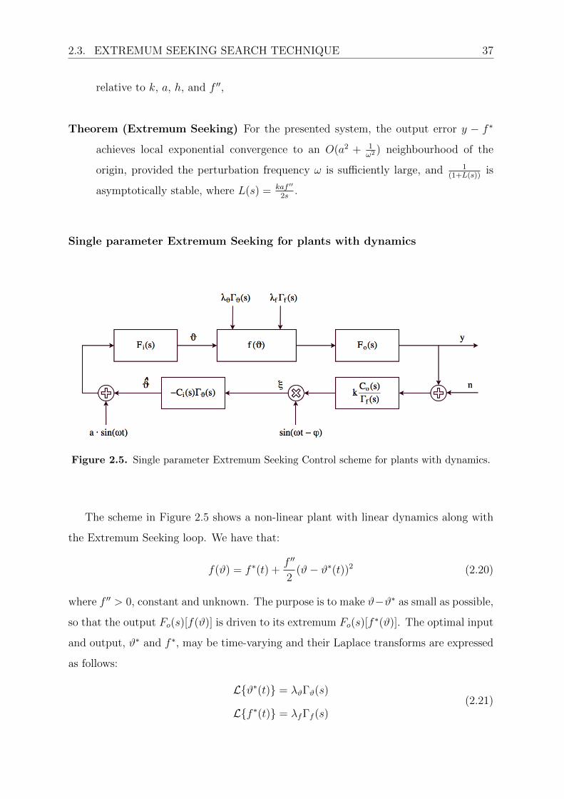
Single parameter Extremum Seeking for plants with dynamics
Figure 2.5. Single parameter Extremum Seeking Control scheme for plants with dynamics.
The scheme in Figure 2.5 shows a non-linear plant with linear dynamics along with
the Extremum Seeking loop. We have that:
f(ϑ) = f ∗(t) +f ′′
2(ϑ− ϑ∗(t))2 (2.20)
where f ′′ > 0, constant and unknown. The purpose is to make ϑ−ϑ∗ as small as possible,
so that the output Fo(s)[f(ϑ)] is driven to its extremum Fo(s)[f∗(ϑ)]. The optimal input
and output, ϑ∗ and f ∗, may be time-varying and their Laplace transforms are expressed
as follows:
Lϑ∗(t) = λϑΓϑ(s)
Lf ∗(t) = λfΓf (s)(2.21)

38 CHAPTER 2. ARTVA SYSTEM AND SEARCH ALGORITHMS
If ϑ∗ and f ∗ are constants, from (2.21) we can find:
Lϑ∗(t) =λϑs
Lf ∗(t) =λfs
(2.22)
While λϑ and λf are unknown, the Laplace transform of ϑ∗ and f ∗ is known, and is
included in the washout filter:Co(s)
Γf (s)=
s
s+ h(2.23)
and in the estimation algorithm:
Ci(s)Γϑ(s) =1
s(2.24)
The inclusion of Γϑ(s) and Γf (s) in the respective blocks in the feedback branch follows
the internal model principle. When applied, in a very generalized manner, to the Ex-
tremum Seeking problem, it allows us to track time-varying maxima or minima.
The compensators Ci(s) and Co(s) are crucial design tools for satisfying stability condi-
tions and achieving desired convergence rates.
2.3.2 Non-local stability of non-linear case
Introduction
Considering the following non-linear system[6]:
x = f(x, u)
y = h(x)(2.25)
and suppose that exist a unique x∗ such that y∗ = h(x∗) is the extremum of the map
h(·). Assume, due to uncertainty, that neither x∗ nor h(·) are precisely known. The
objective is to force the solution of the closed-loop system to eventually converge to x∗
and to do so without any precise knowledge about x∗ or h(·).
The purpose is to show that, under appropriate conditions, the Extremum Seeking con-
troller achieves semi-global practical stability of the closed-loop system. In other words,
given an arbitrarily large set of initial conditions B∆ and an arbitrarily small neigh-
bourhoods Bv of the state x∗ where the output achieves its extremum y∗ = h(x∗), it is

2.3. EXTREMUM SEEKING SEARCH TECHNIQUE 39
possible to adjust the controller parameters so that all solutions starting from the set
B∆ eventually converge to Bv.
Preliminaries
Given the following system:
x = f(t, x, ε) (2.26)
with x ∈ Rn, t ∈ R > 0, ε ∈ Rl > 0, the stability of (2.26) can depend in an intricate
way on the parameters vector ε.
Definition (Semi-Global Practical Asymptotic Stability) System (2.26) is said
to be semi-global practical asymptotically (SPA) stable, uniformly in (ε1, ε2, ..., εj),
j ∈ 1, 2, ..., l, if there exists β ∈ KL such that the following holds: for each pair
of strictly positive real numbers (∆, v), there exist real numbers ε∗k = ε∗k(∆, v) > 0,
k = 1, 2, ..., j, and for each fixed εk ∈ (0, ε∗k), k = 1, 2, ..., j, there exist εi =
εi(ε1, ε2, ..., εi−1,∆, v), with i = j + 1, j + 2, ..., l, such that the solutions of the
system with the so constructed parameters ε = (ε1, ε2, ..., εl) satisfy:
|x(t)| ≤ β(|x0|, (ε1 · ε2 · ... · εl)(t− t0)) + v (2.27)
for all t ≥ t0 ≥ 0, x(t0) = x0, with |x0| ≤ ∆. If we have that j = l, then we can
say that the system is SPA stable, uniformly in ε.
Problem formulation
Considering the following single-input single-output (SISO) non-linear model:
x = f(x, u)
y = h(x)(2.28)
with f : Rn × R→ Rn, f ∈ C, and h : Rn → R, h ∈ C. Considering a family of control
laws of the following form:
u = α(x, ϑ) (2.29)

40 CHAPTER 2. ARTVA SYSTEM AND SEARCH ALGORITHMS
with ϑ ∈ R, scalar parameter. The closed loop system is then:
x = f(x, α(x, ϑ)) (2.30)
The requirement that ϑ is scalar and that the system is SISO is to simplify the presen-
tation.
Assumption 1 There exists a function I : R→ Rn such that
f(x, α(x, ϑ)) = 0 (2.31)
if and only if x = I(ϑ).
Assumption 2 For each ϑ ∈ R, the equilibrium x = I(ϑ) of the closed-loop system is
globally asymptotically stable, uniformly in ϑ.
Assumption 3 Denoting Q(·) = h l, there exists a unique ϑ∗ maximizing Q(·), and
the following holds:
Q′(ϑ∗) = 0, Q′′(ϑ∗) < 0 (2.32)
Main results
Considering the first order Extremum Seeking control scheme shown in Figure 2.6:
Figure 2.6. First order Extremum Seeking control scheme.
The dynamics of the system are the following:
x = f(x, α(x, ϑ+ a · sin(ωt)))
˙ϑ = kh(x)b · sin(ωt)
(2.33)

2.3. EXTREMUM SEEKING SEARCH TECHNIQUE 41
Introducing a change of coordinates:
x = x− x∗
ϑ = ϑ− ϑ∗(2.34)
we note that the point (x∗, ϑ∗) is in general not an equilibrium point of the system.
However, our purpose is to show that the system in new coordinate is SPA stable, which
ensure Extremum Seeking. The system (2.33) with the new coordinates (2.34) takes the
following form:
˙x = f(x+ x∗, α(x+ x∗, ϑ+ ϑ∗ + a · sin(ωt)))
˙ϑ = kh(x+ x∗)b · sin(ωt)(2.35)
Defining now:
k = ωδK
σ = ωt(2.36)
where ω and σ are small parameters, K > 0 is fixed, and replacing (2.36) in (2.35), we
obtain the system equations expanded in time σ:
ωdx
dσ= f(x+ x∗, α(x+ x∗, ϑ+ ϑ∗ + a · sin(σ)))
dϑ
dσ= δKh(x+ x∗)b · sin(σ)
(2.37)
For simplicity of representation, we let b = a, so that the vector of parameters is the
following:
ε = [a2 δ ω]T (2.38)
System (2.37) has a two-time-scale structure and the first main result is proved by
applying the singular perturbations and averaging methods.
Theorem Suppose that assumptions 1-3 hold. Then, the closed-loop system (2.37),
when b = a and with parameter vector (2.38), is SPA stable, uniformly in (a2, δ).
Considering now the higher order Extremum Seeking control scheme represented in Fig-
ure 2.7, supposing WL(s) = (ωl
s+ωl) and WH(s) = 1. The Extremum Seeking controller
contains an integrator and a low-pass filter. The low-pass filter is useful when we need

42 CHAPTER 2. ARTVA SYSTEM AND SEARCH ALGORITHMS
Figure 2.7. Higher order Extremum Seeking control scheme.
to filter out high frequency measurement noise in the system. Moreover, tuning the filer
parameter ωl may lead to a possible improvement in the transient response.
The following equations describe the closed-loop system under the above conditions:
x = f(x, α(x, ϑ+ a · sin(ωt)))
˙ϑ = kξ
ξ = −ωlξ + ωlh(x)a · sin(ωt)
(2.39)
Introducing a change of coordinates:
x = x− x∗
ϑ = ϑ− ϑ∗
ξ = ξ
(2.40)
system (2.39) with the new coordinates (2.40) takes the following form:
˙x = f(x+ x∗, α(x+ x∗, ϑ+ ϑ∗ + a · sin(ωt)))
˙ϑ = kξ
˙ξ = −ωl[ξ − h(x+ x∗)a · sin(ωt)]
(2.41)
Defining now:
ωl = ωδωL
k = ωδK
σ = ωt
(2.42)

2.3. EXTREMUM SEEKING SEARCH TECHNIQUE 43
where ω and σ are small parameters, ωL and K > 0 are fixed, and replacing (2.42) in
(2.41), we obtain the system equations expanded in time σ:
ωdx
dσ= f(x+ x∗, α(x+ x∗, ϑ+ ϑ∗ + a · sin(σ)))
dϑ
dσ= δKξ
dξ
dσ= −δωL[ξ − h(x+ x∗)a · sin(σ)]
(2.43)
With the same parameter vector ε defined in (2.38)
Theorem Suppose that assumptions 1-3 hold. Then, the closed-loop system (2.43),
with parameter vector (2.38), is SPA stable, uniformly in a2.
2.3.3 Hybrid Extremum Seeking Control
The next presented algorithm is based on an Hybrid Extremum Seeking Control
(HESC). An hybrid dynamical system[7] is modelled as follows:
x ∈ C x = f(x)
x ∈ D x+ = g(x)(2.44)
The state x of the hybrid system can change according to a differential equation x = f(x)
and according to a difference equation x+ = g(x). The behaviour of a dynamical system
which can be described by a differential equation is referred to as flow, while the behaviour
of a dynamical system which can be described by a difference equation is referred to as
jump. The objects involved in model (2.44) are:
• the flow set C,
• the flow map f ,
• the jump set D,
• the jump map g.
Considering now the model of the HESC[8], and assuming that the time domain is
described by continuous-time interval parametrized by τ ∈ [0, T ), with T > 0, and

44 CHAPTER 2. ARTVA SYSTEM AND SEARCH ALGORITHMS
discrete-time instants j ∈ N, the flow map is described by the following equations:
˙px = vx
˙vx = −k1xvx − k2xwx
˙wx = 0
˙py = vy
˙vy = −k1yvy − k2ywy
˙wy = 0
h∗ = 0
ψ∗ = 0
τ = 1
(2.45)
where k1x, k2x, k1y and k2y are positive constants to be defined. The flow set is defined
as:
( ˙px, ˙vx, ˙wx, ˙py, ˙vy, ˙wy, h∗, ψ∗), τ ∈ R8 × [0, T ) (2.46)
Indicating with d the distance values and with δ the angle values obtained from ARTVA,
the jump map is described as follows:
px+ = px
vx+ = vx
wx+ =
1
n
j∑i=j+1−n
d(i) sin(iωxT )
py+ = py
vy+ = vy
wy+ =
1
n
j∑i=j+1−n
d(i) sin(iωyT )
h∗+ = h∗
ψ∗+ = ψ + δ
τ+ = 0
(2.47)
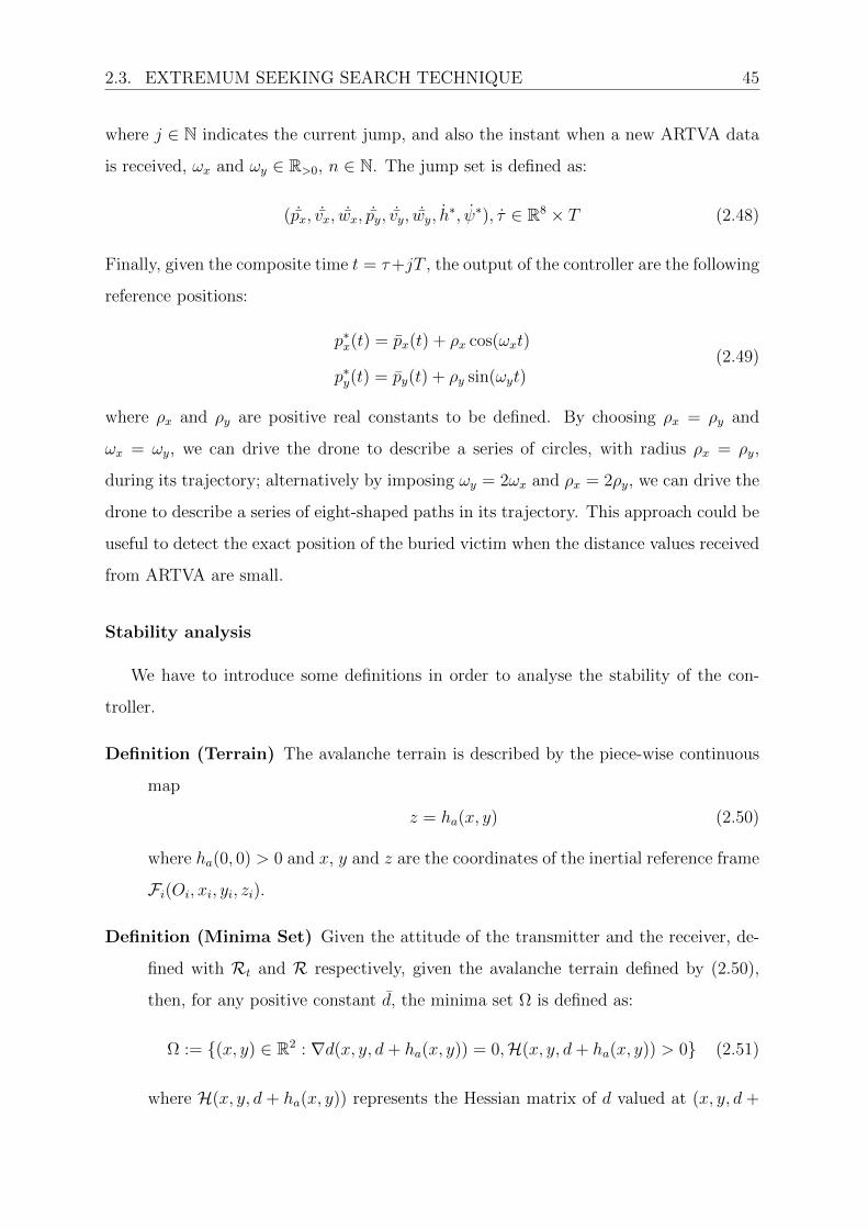
2.3. EXTREMUM SEEKING SEARCH TECHNIQUE 45
where j ∈ N indicates the current jump, and also the instant when a new ARTVA data
is received, ωx and ωy ∈ R>0, n ∈ N. The jump set is defined as:
( ˙px, ˙vx, ˙wx, ˙py, ˙vy, ˙wy, h∗, ψ∗), τ ∈ R8 × T (2.48)
Finally, given the composite time t = τ+jT , the output of the controller are the following
reference positions:
p∗x(t) = px(t) + ρx cos(ωxt)
p∗y(t) = py(t) + ρy sin(ωyt)(2.49)
where ρx and ρy are positive real constants to be defined. By choosing ρx = ρy and
ωx = ωy, we can drive the drone to describe a series of circles, with radius ρx = ρy,
during its trajectory; alternatively by imposing ωy = 2ωx and ρx = 2ρy, we can drive the
drone to describe a series of eight-shaped paths in its trajectory. This approach could be
useful to detect the exact position of the buried victim when the distance values received
from ARTVA are small.
Stability analysis
We have to introduce some definitions in order to analyse the stability of the con-
troller.
Definition (Terrain) The avalanche terrain is described by the piece-wise continuous
map
z = ha(x, y) (2.50)
where ha(0, 0) > 0 and x, y and z are the coordinates of the inertial reference frame
Fi(Oi, xi, yi, zi).
Definition (Minima Set) Given the attitude of the transmitter and the receiver, de-
fined with Rt and R respectively, given the avalanche terrain defined by (2.50),
then, for any positive constant d, the minima set Ω is defined as:
Ω := (x, y) ∈ R2 : ∇d(x, y, d+ ha(x, y)) = 0,H(x, y, d+ ha(x, y)) > 0 (2.51)
where H(x, y, d + ha(x, y)) represents the Hessian matrix of d valued at (x, y, d +

46 CHAPTER 2. ARTVA SYSTEM AND SEARCH ALGORITHMS
ha(x, y)).
Definition (Minima Domain) For each element (x, y) ∈ Ω, the minima domain D(x,y)
is defined as the compact set
D(x,y) :=
(x, y) ∈ R2 : ∇d(x−x, y−y, d+ha(x−x, y−y))×
x− xy − y
> 0
(2.52)
where (x, y) ∈ D(x,y).
The validity of the HESC is based on the following assumptions:
Assuption (Periodicity) The pulsations ωx and ωy and the number of samples n are
such that
1
n
j∑i=j+1−n
sin(iωxT ) = 0
1
n
j∑i=j+1−n
sin(iωyT ) = 0
(2.53)
Assuption (Persistent Excitation) The pulsations ωx and ωy are such that there
exist two positive constants αx and αy such that
1
n
j∑i=j+1−n
sin2(iωxT ) > αx
1
n
j∑i=j+1−n
sin2(iωyT ) > αy
(2.54)
and furthermore1
n
j∑i=j+1−n
sin(iωxT ) sin(iωyT ) = 0 (2.55)
Now we can conclude that:
Theorem Given the HESC controller (2.45)-(2.47) and the position of the drone defined
by p = [p∗x, p∗y, d + ha(x, y)], and assuming ||w|| = 0, then, for any ρ > 0 such that
Bρ(x, y) ⊂ D(x,y), there exist two positive constants ρx and ρy such that, for any
(ρ∗x(0), ρ∗y(0)) ∈ Bρ(x, y) and for all 0 < ρx < ρx and 0 < ρy < ρy, the point (x, y)
is locally asymptotically stable.

2.3. EXTREMUM SEEKING SEARCH TECHNIQUE 47
The term Bρ(x, y) indicates a ball of radius ρ.
Remark This result says that, if p∗(t) ∈ D(x,y) for all t ≥ 0, then the average position
(ρx, ρy) asymptotically goes to (x, y).
2.3.4 Implementation
The HESC set-point generation algorithm follows the steps below:
FIFO update Stores a first in first out (FIFO) queue of the last m distance values
received from ARTVA and update it each time new data arrive.
Direction check Works a bit differently with respect to its counterpart in the previous
algorithm: takes an arithmetic mean of the last ck valid values found and, after dk
data received, compares the distance value of the last found data with the computed
mean. If the new value is greater than the mean, changes sign to the formula that
computes the set-point. The choice of computing the mean of ck values and to
wait dk data before performing the check is due to the fact that the imposed circle-
shaped (or eight-shaped, alternatively) trajectory results in consecutive distance
values which are not always decreasing, even if the drone is moving in the right
direction. Both ck and dk are tunable coefficients.
Yaw correction Exactly like the previous presented algorithm, computes the yaw cor-
rection to be applied to the drone if the angle values received from ARTVA is
greater than a certain threshold:
if angle value > threshold then apply the yaw correction
The yaw correction is saturated to a maximum value in such a way to be applied
gradually each time a new set-point is given to the controller:
if angle value ≤ yaw correction max then yaw correction = angle value
else yaw correction = yaw correction max
In this way, we avoid to have non-consistent consecutive ARTVA measures, which
will create difficulties in the data validation phase.
48 CHAPTER 2. ARTVA SYSTEM AND SEARCH ALGORITHMS
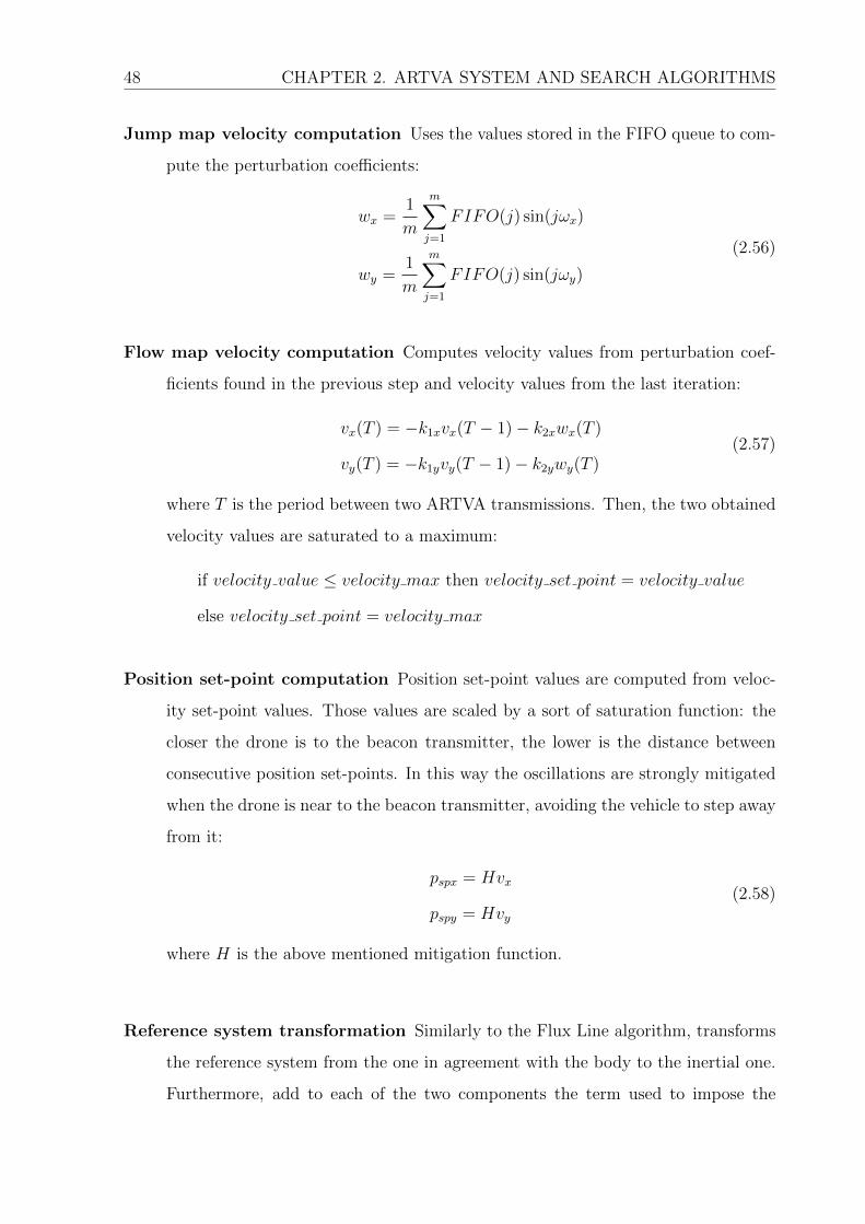
Jump map velocity computation Uses the values stored in the FIFO queue to com-
pute the perturbation coefficients:
wx =1
m
m∑j=1
FIFO(j) sin(jωx)
wy =1
m
m∑j=1
FIFO(j) sin(jωy)
(2.56)
Flow map velocity computation Computes velocity values from perturbation coef-
ficients found in the previous step and velocity values from the last iteration:
vx(T ) = −k1xvx(T − 1)− k2xwx(T )
vy(T ) = −k1yvy(T − 1)− k2ywy(T )(2.57)
where T is the period between two ARTVA transmissions. Then, the two obtained
velocity values are saturated to a maximum:
if velocity value ≤ velocity max then velocity set point = velocity value
else velocity set point = velocity max
Position set-point computation Position set-point values are computed from veloc-
ity set-point values. Those values are scaled by a sort of saturation function: the
closer the drone is to the beacon transmitter, the lower is the distance between
consecutive position set-points. In this way the oscillations are strongly mitigated
when the drone is near to the beacon transmitter, avoiding the vehicle to step away
from it:
pspx = Hvx
pspy = Hvy
(2.58)
where H is the above mentioned mitigation function.
Reference system transformation Similarly to the Flux Line algorithm, transforms
the reference system from the one in agreement with the body to the inertial one.
Furthermore, add to each of the two components the term used to impose the
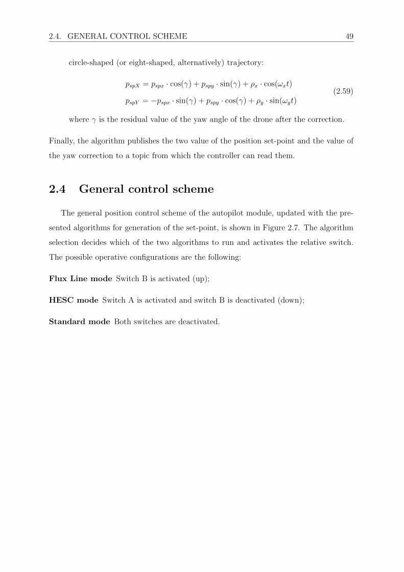
2.4. GENERAL CONTROL SCHEME 49
circle-shaped (or eight-shaped, alternatively) trajectory:
pspX = pspx · cos(γ) + pspy · sin(γ) + ρx · cos(ωxt)
pspY = −pspx · sin(γ) + pspy · cos(γ) + ρy · sin(ωyt)(2.59)
where γ is the residual value of the yaw angle of the drone after the correction.
Finally, the algorithm publishes the two value of the position set-point and the value of
the yaw correction to a topic from which the controller can read them.
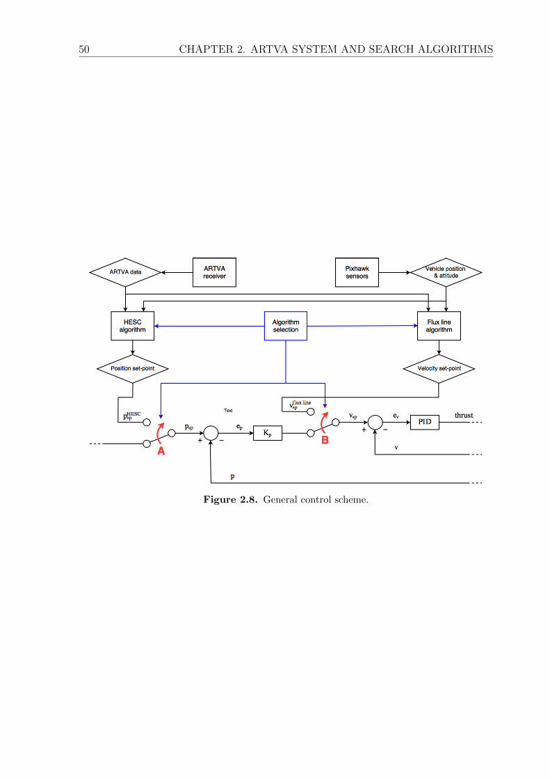
2.4 General control scheme
The general position control scheme of the autopilot module, updated with the pre-
sented algorithms for generation of the set-point, is shown in Figure 2.7. The algorithm
selection decides which of the two algorithms to run and activates the relative switch.
The possible operative configurations are the following:
Flux Line mode Switch B is activated (up);
HESC mode Switch A is activated and switch B is deactivated (down);
Standard mode Both switches are deactivated.
50 CHAPTER 2. ARTVA SYSTEM AND SEARCH ALGORITHMS
Figure 2.8. General control scheme.

Chapter 3
Results
Below we will analyse the results of the simulations of the two presented search
algorithms, and the main issues related to the practical implementation of the system.
3.1 Simulations
The software used to simulate the two algorithms is Robot Operating System (ROS),
the main functionalities of which are discussed in the first appendix. The simulations
are realized by means of three different ROS nodes:
Drone and ARTVA simulator Simulate both the model of the drone, with its dy-
namical behaviour, and the ARTVA beacon transmitter. The ARTVA equivalent
model[8] is obtained considering the nominal magnetic field generated, represented
in (2.3), and the magnetic field intensity described by:
||H|| = ||m||4π||r||3
√1 + 3 cos2 Θ (3.1)
where the actual distance to the transmitter is indicated by the vector r, while
Θ ∈ [0, π] describes the angle between r and m. Given rmin ∈ R>0 and rmax ∈ R>0,
with rmin < rmax, we can define the three operation zones:
• the outer zone:
Zo := p ∈ R3 : ||p− pt|| > rmax
51

52 CHAPTER 3. RESULTS
• the mid zone:
Zm := p ∈ R3 : rmin < ||p− pt|| ≤ rmax
• and the inner zone:
Zi := p ∈ R3 : ||p− pt|| ≤ rmin
where p and pt are the positions of the receiver and the transmitter, respectively.
From (2.3), the value of distance d, output of the receiver, can be approximated in
the following way:
d =
(keq
4π‖C(RTH + w)‖
) 13
(3.2)
where keq is a positive constant, R is the receiver orientation, and C is a selection
matrix that assumes two different values, CP2 and CP3:
CP2 = [1 0 0]
CP3 = I3×3
leading so to two possible distance calculations, namely dP2 and dP3. The receiver
first determines the distance dP3 and, if dP3 < 300, sets the angle δ(k) to zero and
d(k) = dP3, otherwise calculates the distance dP2. If dP2 < 5000, then the receiver
determines the δ angle by means of the following equation:
δ = tan−1
([0 1 0](RTH + w)
[1 0 0](RTH + w)
)(3.3)
and imposes d(k) = dP2. Lastly, if dP2 > 5000, the receiver’s output is d(k) = −1
and δ(k) = 0. The vector w = [wbx wby wbz]T represents the electromagnetic
interferences, expressed in body frame, and can be written as sum of drone noises,
wd, and environmental noises we.
In the end, both d and δ, obtained from (3.2) and (3.3), are discretised and sampled
by means of a standard zero-hold filter to simulate their digital nature.
Set-point generation algorithm Contain the implementation of the algorithm (Flux
Line or HESC).
Controller simulator Simulate a simple discrete integrator.
3.1. SIMULATIONS 53
To perform the simulation, the three nodes has to be run in parallel on three different
terminal windows. We will present the results of the simulation of four different cases in
which, while the simulated drone is always initially placed at the origin of the inertial
reference frame, with the body frame coincident with it, the simulated transmitter is
placed in different spots:
• Case A: transmitter at (10, 15,−2);
• Case B: transmitter at (−6, 16,−2);
• Case C: transmitter at (−14,−9,−2);
• Case D: transmitter at (12,−13,−2).
The distance unit represents a metre, thus, in each case, the simulated transmitter is
more or less 17 metres far from the simulated drone and 2 metres under the snow.
3.1.1 Flux Line algorithm simulation
The output positions of the simulated drone, obtained by means of set-points gener-
ated with Flux Line search algorithm, and collected at each integration step, are plotted
in Figures 3.1-4. The algorithm performs quite well, with the simulated drone going
straight toward the transmitter’s position and reaching it with a good precision. Once
it gets to the minimum distance point, the simulated drone starts moving forward and
backward on the same line, remaining in the neighbourhood of the target. This is due
to the direction check step of the algorithm, which imposes to the vehicle a velocity
set-point equal to the last one but with opposite sign each time the drone steps away
from the transmitter’s position, and to the fact that, when the drone is very close to the
transmitter, the received angle value is zero, and so the yaw correction step does not
intervene, forcing the vehicle to maintain always the same orientation. Moreover, thanks
to the saturation of the velocity, the vehicle will move slowly when the detected distance
is small, avoiding so to go too far from the target.

54 CHAPTER 3. RESULTS
Figure 3.1. Flux Line algorithm simulation case A: transmitter at (10, 15,−2), the black dot
represents the initial position of the drone, the blue line represents the drone trajectory, the
red cross represents the transmitter’s position.
Figure 3.2. Flux Line algorithm simulation case B: transmitter at (−6, 16,−2), the black dot
represents the initial position of the drone, the blue line represents the drone trajectory, the
red cross represents the transmitter’s position.

3.1. SIMULATIONS 55
Figure 3.3. Flux Line algorithm simulation case C: transmitter at (−14,−9,−2), the black
dot represents the initial position of the drone, the blue line represents the drone trajectory,
the red cross represents the transmitter’s position.
Figure 3.4. Flux Line algorithm simulation case D: transmitter at (12,−13,−2), the black
dot represents the initial position of the drone, the blue line represents the drone trajectory,
the red cross represents the transmitter’s position.

56 CHAPTER 3. RESULTS
3.1.2 HESC algorithm simulation
Same as before, the output positions of the simulated drone, obtained this time
by means of set-points generated with circle-shaped HESC search algorithm and eight-
shaped HESC search algorithm, and collected at each integration step, are plotted in
Figures 3.5-8 and 3.9-12 respectively. Also this algorithm performs well, with the simu-
lated drone moving toward the transmitter’s position with the imposed oscillating move-
ment. The more the vehicle gets closer to the target, the more the trajectory takes the
geometry of a series of circles (or a series of eight-shaped paths, alternatively). Once
it gets close to the transmitter’s position, the drone continues oscillating, remaining in
its neighbourhood. This is due to the mitigation function, which reduces the imposed
perturbations, and so the velocity of the vehicle, the closer it gets to the target, and to
the direction check step of the algorithms, which reverses the motion if the drone goes
to far from the transmitter’s position.
Figure 3.5. Circle-shaped HESC algorithm simulation case A: transmitter at (10, 15,−2),
the black dot represents the initial position of the drone, the blue line represents the drone
trajectory, the red cross represents the transmitter’s position.

3.1. SIMULATIONS 57
Figure 3.6. Circle-shaped HESC algorithm simulation case B: transmitter at (−6, 16,−2),
the black dot represents the initial position of the drone, the blue line represents the drone
trajectory, the red cross represents the transmitter’s position.
Figure 3.7. Circle-shaped HESC algorithm simulation case C: transmitter at (−14,−9,−2),
the black dot represents the initial position of the drone, the blue line represents the drone
trajectory, the red cross represents the transmitter’s position.

58 CHAPTER 3. RESULTS
Figure 3.8. Circle-shaped HESC algorithm simulation case D: transmitter at (12,−13,−2),
the black dot represents the initial position of the drone, the blue line represents the drone
trajectory, the red cross represents the transmitter’s position.
Figure 3.9. Eight-shaped HESC algorithm simulation case A: transmitter at (10, 15,−2),
the black dot represents the initial position of the drone, the blue line represents the drone
trajectory, the red cross represents the transmitter’s position.

3.1. SIMULATIONS 59
Figure 3.10. Eight-shaped HESC algorithm simulation case B: transmitter at (−6, 16,−2),
the black dot represents the initial position of the drone, the blue line represents the drone
trajectory, the red cross represents the transmitter’s position.
Figure 3.11. Eight-shaped HESC algorithm simulation case C: transmitter at (−14,−9,−2),
the black dot represents the initial position of the drone, the blue line represents the drone
trajectory, the red cross represents the transmitter’s position.

60 CHAPTER 3. RESULTS
Figure 3.12. Eight-shaped HESC algorithm simulation case D: transmitter at (12,−13,−2),
the black dot represents the initial position of the drone, the blue line represents the drone
trajectory, the red cross represents the transmitter’s position.
3.1.3 Algorithms comparison
Now we will show a comparison between the two new proposed algorithms and the
Cross Flight algorithm described in the first chapter of this document, focusing on the
time they take to drive the simulated drone to the transmitter’s position, in such a way
to highlights their performance. For each algorithm, four simulations has been run using
the four cases of transmitter’s position presented before; the results of those simulations,
namely the time each algorithm takes for each single run and the average time, are
reported in Table 3.1. The maximum reference velocity imposed for each algorithm is
2 m/s. Furthermore, for Flux Line and HESC algorithms the simulation stops as soon
as the drone gets close to the transmitter (d < 250), while the Cross Flight algorithm
simulation stops when it reaches the computed position.
It is straightforward to see that Flux Line and HESC algorithms performs much better
than Cross Flight. Moreover, we can state that Flux Line is slightly faster than HESC
algorithms, mainly because of the oscillating trajectory of the seconds with respect to
the straight one of the first.

3.2. PRACTICAL IMPLEMENTATION 61
Search algorithm Case A Case B Case C Case D Average
Flux Line 29.62 33.58 31.59 28.55 30.84
Circle-shaped HESC 45.45 43.45 41.03 46.93 44.22
Eight-shaped HESC 45.39 42.51 42.45 45.35 43.93
Cross Flight 117.54 140.70 114.20 106.16 119.65
Table 3.1. Algorithms comparison: the time is expressed in seconds; case A: (10, 15,−2), case
B: (−6, 16,−2), case C: (−14,−9,−2), case D: (12,−13,−2).
3.2 Practical implementation
Regarding the practical implementation, it has been possible to test the operation of
the ARTVA system under different conditions. Nevertheless, we are not been able to test
the two presented search algorithms, both because some additional control structures are
needed, like take-off, landing and altitude management, and because of issues related to
ARTVA system implementation.
The main problem is the electromagnetic noise produced by brushless motors and by
the modulation technique adopted for the electronic speed controllers (ESCs). These
electromagnetic disturbances are low frequency signals, and when their intensity is high
enough, the ARTVA receiver sees them, and consequently handles them, as ARTVA
transmitter’s signals. By carrying out several tests under different conditions, as said
before, we have been able to observe the capability of ARTVA system and the behaviour
of electromagnetic disturbances. The tests made can be categorized as follows:
• motors off;
• motors on, without shielding;
• motors on, with standard aluminium shielding;
• motors on, with EMI aluminium shielding.
3.2.1 Test with motors off
The first test has been taken with motors off, and had the aim to verify the actual
range of the ARTVA system. The values of the received distance measures, related to

62 CHAPTER 3. RESULTS
the actual distance between the transmitter and the receiver, are reported in Table 3.2.
We can state that the progression of the ARTVA distance values are quite linear with
respect to actual distances, with a couple of exceptions. In particular, the value read
at 6 metres is higher than the one read at 8 metres, so it could be a wrong measure,
and the range of values read at 12 metres are too high, so they must be some kind of
disturbance. Furthermore, it is easy to note that the more is the distance between the
transmitter and the receiver, the higher is the variance of the measures obtained at the
same distance (e.g. values read at 22 metres). So, we can conclude that the system is
reliable within a distance of about 20 metres.
Actual distance (metres) ARTVA distance value
0 53
2 425
4 545
6 746
8 729
10 805
12 1838 / 1974
14 1036 / 1053
16 1242 / 1276
18 1648 / 1674
20 2140 / 2200
22 2140 / 2701
Table 3.2. Test results: motors off.
3.2.2 Test with motors on and no shielding
Another test has been taken with motors on, without propellers and with a constant
throttle of about 25%, so to verify the effect of the magnetic disturbances on the measure.
The results are reported in Table 3.3. It is immediate to see that with motors on we have
a drastic decrease in the quality of the measurement. Indeed, at distance greater than
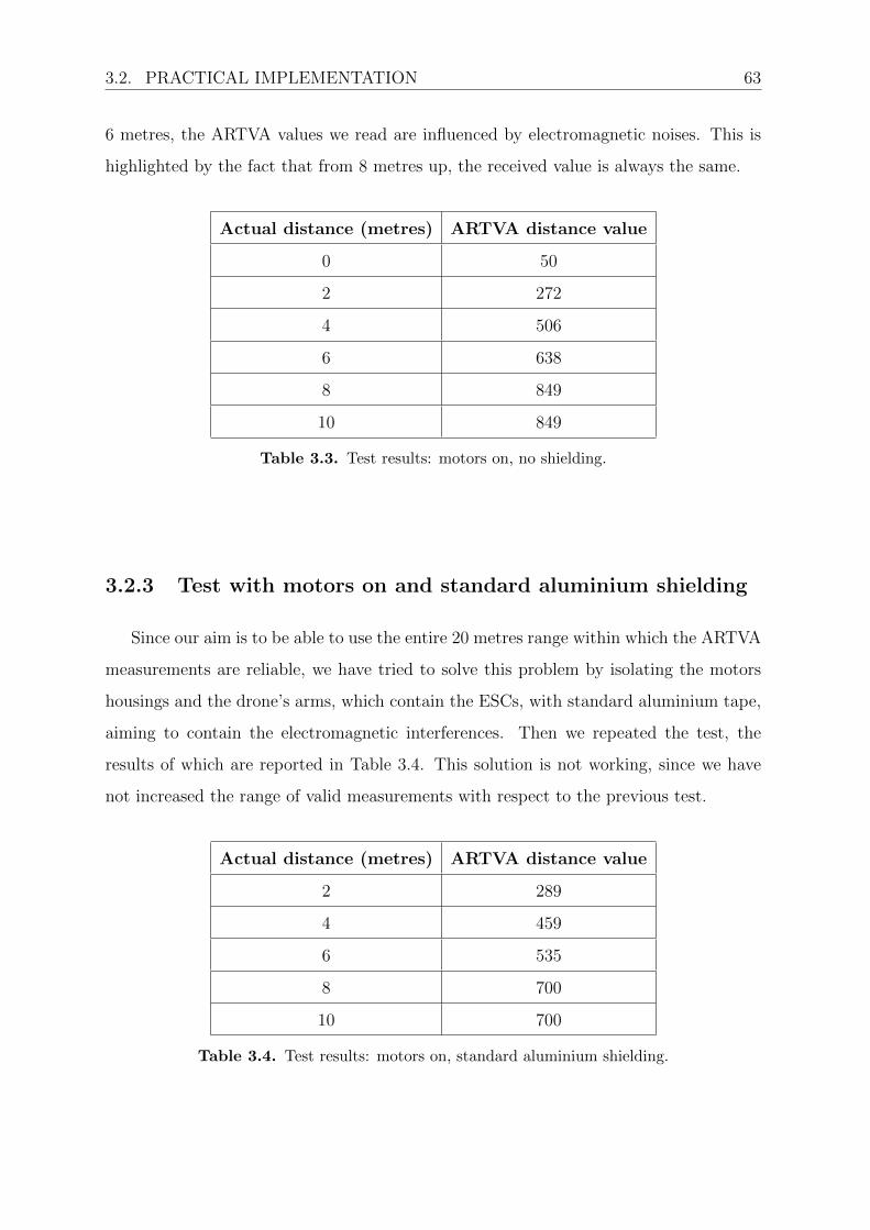
3.2. PRACTICAL IMPLEMENTATION 63
6 metres, the ARTVA values we read are influenced by electromagnetic noises. This is
highlighted by the fact that from 8 metres up, the received value is always the same.
Actual distance (metres) ARTVA distance value
0 50
2 272
4 506
6 638
8 849
10 849
Table 3.3. Test results: motors on, no shielding.
3.2.3 Test with motors on and standard aluminium shielding
Since our aim is to be able to use the entire 20 metres range within which the ARTVA
measurements are reliable, we have tried to solve this problem by isolating the motors
housings and the drone’s arms, which contain the ESCs, with standard aluminium tape,
aiming to contain the electromagnetic interferences. Then we repeated the test, the
results of which are reported in Table 3.4. This solution is not working, since we have
not increased the range of valid measurements with respect to the previous test.
Actual distance (metres) ARTVA distance value
2 289
4 459
6 535
8 700
10 700
Table 3.4. Test results: motors on, standard aluminium shielding.

64 CHAPTER 3. RESULTS
3.2.4 Test with motors on and EMI aluminium shielding
Finally, we have tried to repeat the isolation solution using an electromagnetic inter-
ference (EMI) shielding aluminium tape, instead of a standard one. So we have isolated
the motors housings and the drone’s arms with the EMI aluminium tape, and then we
have repeated the test. The results are shown in Table 3.5. We have obtained just a
slight improvement in the quality of the measure (about 2 metres), which is absolutely
not enough for our purposes. This suggests that, despite the total isolation, there is still
an escape route for electromagnetic disturbances.
Actual distance (metres) ARTVA distance value
2 343
4 506
6 545
8 621
10 700
12 700
Table 3.5. Test results: motors on, EMI aluminium shielding.
Conclusions
Avalanche beacon systems are very helpful devices for the intent of saving people
buried under snow due to avalanches. Their implementation on aerial robots can lead
to even better results, speeding up search operations, ensuring so a faster human inter-
vention and raising the chances of finding missing people still alive and in non-critical
conditions.
In this thesis, we have analysed two search algorithms, based on the data received by
the avalanche beacon transmitter, aiming to improve the search time even more. The
innovation proposed by these two algorithms, with respect to the ones that have been
proposed until now, is that, as soon as the beacon signal is caught, the quad-copter drone
is guided directly toward the victim. From simulations performed with ROS, we observed
that both the proposed algorithms performs quite well, leading the drone straight toward
the signal source, and making it remain in the neighbourhood of the ARTVA transmitter
once find it.
Nevertheless, we have stumbled in some problems which arise with the practical imple-
mentation of this system. In particular, the electromagnetic noises coming from motors
and ESCs mounted on the quad-copter. These disturbances heavily influence the mea-
sures received from ARTVA, significantly decreasing the reliability of the system. As a
consequence of this, only the measures obtained around a few metres from the beacon
transmitter are correct, while, beyond a certain threshold, all the read values are in-
deed influenced by the electromagnetic noise. In this way, the efficiency of the presented
search algorithms is nullified, since we need to get very close to the ARTVA transmitter
in order to get a useful measure. We have tried to handle this issue by isolating the
disturbance generating components with a standard aluminium tape first, and then with
a EMI aluminium tape, unfortunately obtaining unsatisfactory results.
65

66 CONCLUSIONS
A possible future development to make the algorithms usable is to change the mechanical
configuration of the quad-copter drone; e.g. moving the motors and the ESCs in a cen-
tral aluminium housing, positioning the motors in such a way that the rotating axes are
horizontal, and transmitting the motion to the propellers by means of shafts supported
by spherical bearings, mounted inside the drone’s arms, at the end of which are placed
spiral bevel gears, in such a way to turn by 90 degrees the direction of the rotating axes.

Appendix A
First Appendix
Here are reported the description of some basis concepts, software structures and
tools that have been used in the project.
A.1 PX4
PX4 is the software running on the Pixhawk autopilot module. It consists in two
main layers[9]: the flight stack, which is an estimation and flight control system, and the
middleware, which is a general robotics layer that can support any type of autonomous
robot, providing internal/external communications and hardware integration. Modules
communicate with each other through a publish-subscribe message bus named uORB.
PX4 code runs on a real-time operating system (RTOS) named NuttX.
A.1.1 Flight stack
The flight stack is a collection of guidance, navigation and control algorithms for
autonomous drones. Figure A.1 shows an overview of the building blocks of the flight
stack. The estimator takes one or more sensor inputs and combines them to compute
a vehicle state. The controller takes a set-point and a measurement or estimated state
as input and adjust the value of the process variable such that it matches the set-point;
the output is a correction to eventually reach that set-point. The mixer takes force
commands and translates them into individual motor commands, while ensuring that
some limits are not exceeded.
67
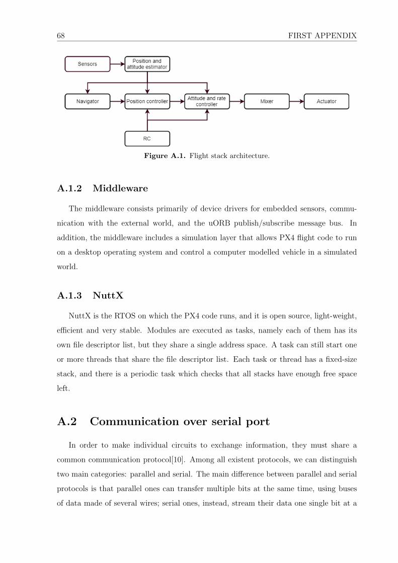
68 FIRST APPENDIX
Figure A.1. Flight stack architecture.
A.1.2 Middleware
The middleware consists primarily of device drivers for embedded sensors, commu-
nication with the external world, and the uORB publish/subscribe message bus. In
addition, the middleware includes a simulation layer that allows PX4 flight code to run
on a desktop operating system and control a computer modelled vehicle in a simulated
world.
A.1.3 NuttX
NuttX is the RTOS on which the PX4 code runs, and it is open source, light-weight,
efficient and very stable. Modules are executed as tasks, namely each of them has its
own file descriptor list, but they share a single address space. A task can still start one
or more threads that share the file descriptor list. Each task or thread has a fixed-size
stack, and there is a periodic task which checks that all stacks have enough free space
left.
A.2 Communication over serial port
In order to make individual circuits to exchange information, they must share a
common communication protocol[10]. Among all existent protocols, we can distinguish
two main categories: parallel and serial. The main difference between parallel and serial
protocols is that parallel ones can transfer multiple bits at the same time, using buses
of data made of several wires; serial ones, instead, stream their data one single bit at a
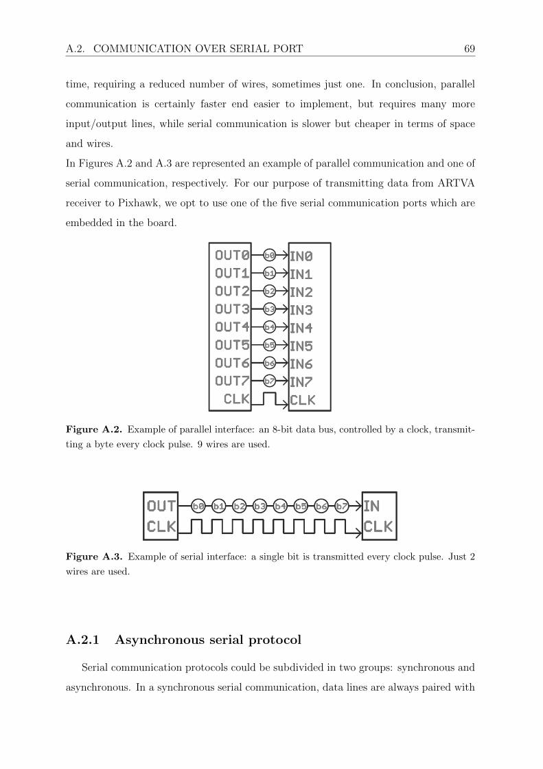
A.2. COMMUNICATION OVER SERIAL PORT 69
time, requiring a reduced number of wires, sometimes just one. In conclusion, parallel
communication is certainly faster end easier to implement, but requires many more
input/output lines, while serial communication is slower but cheaper in terms of space
and wires.
In Figures A.2 and A.3 are represented an example of parallel communication and one of
serial communication, respectively. For our purpose of transmitting data from ARTVA
receiver to Pixhawk, we opt to use one of the five serial communication ports which are
embedded in the board.
Figure A.2. Example of parallel interface: an 8-bit data bus, controlled by a clock, transmit-
ting a byte every clock pulse. 9 wires are used.
Figure A.3. Example of serial interface: a single bit is transmitted every clock pulse. Just 2
wires are used.
A.2.1 Asynchronous serial protocol
Serial communication protocols could be subdivided in two groups: synchronous and
asynchronous. In a synchronous serial communication, data lines are always paired with

70 FIRST APPENDIX
a clock signal in such a way that all connected devices shares the same clock. This will
result in a more straightforward and faster transmission, but it requires at least an extra
wire between communicating devices. Conversely, asynchronous serial communications
does not need the support of an external clock, minimizing so the required wires, but
requiring more effort in ensuring the reliability of the transferring and receiving data.
The protocol that we use for our purpose is the most common form of asynchronous
serial communication.
A.2.2 Rules of serial communication
The asynchronous serial communication protocol presents a series of mechanisms with
specific rules, which help ensuring robust and error-free data transfers, compensating the
lack of the external clock. These mechanisms are:
• data bits,
• synchronization bits,
• parity bits,
• and baud rate.
The protocol is highly configurable and there are several way to transfer data serially;
the critical part is to ensure that both the communicating devices are configured to use
the exact same protocol.
Data block The data block contains the information carried by the serial packet. A
single packet can be set to contain from 5 to 9 bits of data. The standard data
size is the basic 8-bit byte. Other than on the single character-length, the two
connected device must agree also on the endianness of the data. In big-endian the
most significant byte, namely the one containing the most significant bit, is stored
or sent first, and then the following bytes are stored or sent in decreasing significant
order; vice versa in little-endian.
Synchronization bits The synchronization bits are special kind of bits, a start bit
and one or two stop bits, which are used to mark, as their names suggest, at the
beginning and at the end of the packet respectively.
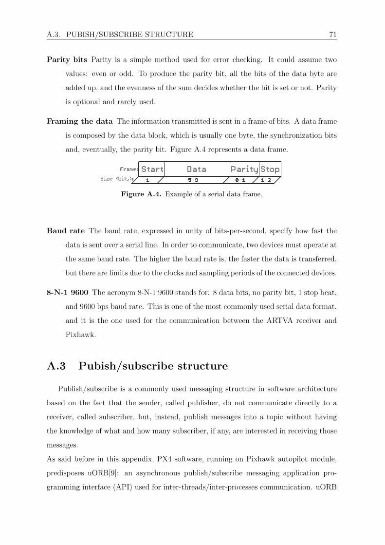
A.3. PUBISH/SUBSCRIBE STRUCTURE 71
Parity bits Parity is a simple method used for error checking. It could assume two
values: even or odd. To produce the parity bit, all the bits of the data byte are
added up, and the evenness of the sum decides whether the bit is set or not. Parity
is optional and rarely used.
Framing the data The information transmitted is sent in a frame of bits. A data frame
is composed by the data block, which is usually one byte, the synchronization bits
and, eventually, the parity bit. Figure A.4 represents a data frame.
Figure A.4. Example of a serial data frame.
Baud rate The baud rate, expressed in unity of bits-per-second, specify how fast the
data is sent over a serial line. In order to communicate, two devices must operate at
the same baud rate. The higher the baud rate is, the faster the data is transferred,
but there are limits due to the clocks and sampling periods of the connected devices.
8-N-1 9600 The acronym 8-N-1 9600 stands for: 8 data bits, no parity bit, 1 stop beat,
and 9600 bps baud rate. This is one of the most commonly used serial data format,
and it is the one used for the communication between the ARTVA receiver and
Pixhawk.
A.3 Pubish/subscribe structure
Publish/subscribe is a commonly used messaging structure in software architecture
based on the fact that the sender, called publisher, do not communicate directly to a
receiver, called subscriber, but, instead, publish messages into a topic without having
the knowledge of what and how many subscriber, if any, are interested in receiving those
messages.
As said before in this appendix, PX4 software, running on Pixhawk autopilot module,
predisposes uORB[9]: an asynchronous publish/subscribe messaging application pro-
gramming interface (API) used for inter-threads/inter-processes communication. uORB

72 FIRST APPENDIX
is automatically started when the PX4 software is executed, since many applications
depend on it.
The main elements of the uORB messaging API are:
• topic,
• publisher,
• subscriber.
Below it is described how to enable uORB messaging between PX4 modules.
A.3.1 Adding a new topic
To add a new topic, it is sufficient to create a .msg file, containing the variables
that we want to pass from a module to another, inside the /msg directory of the PX4
software, and add the .msg file name to the list present in the file msg/Cmakelist.txt,
which is also present in the /msg directory. This procedure will automatically generate
the topic at build time, which will be placed in the /uORB/topics directory and has
the form of a structure. To use a topic in a PX4 module, it is necessary to include the
following header:
#include <uORB/topics/topic_name.h>
A.3.2 Publish into a topic
To publish a message into a topic from a PX4 module, after having included the topic
header to the module as shown above, the first thing to do is to declare the publisher
variable, which is used just to advertise the topic, and the structure to publish into the
topic:
orb_advert_t topic_name_pub;
struct topic_name_s topic_data;
Then it is necessary to advertise the topic:
topic_name_pub = orb_advertise(ORB_ID(topic_name), &topic_data);

A.3. PUBISH/SUBSCRIBE STRUCTURE 73
Finally, it is possible to publish the variable of the structure into the topic at any point
of the execution of the module by means of the following code string:
orb_publish(ORB_ID(topic_name), topic_name_pub, &topic_data);
After that, the variables are saved into the topic and could be used into another module
by subscribing it to that topic.
A.3.3 Subscribe to a topic
To make a PX4 module subscribe to a topic, in order to take values provided or
computed by another module, after having included the topic header, we have to declare
the subscriber variable, which is used to subscribe to the topic, the structure in which
we want to save the variables taken from the topic, and a boolean variable used to check
if the topic has been updated since last time it was checked:
int topic_name_sub;
struct topic_name_s topic_data;
bool updated;
Then we must subscribe to the topic:
topic_name_sub = orb_subscribe(ORB_ID(topic_name));
Lastly, it is possible, at any point of the execution of the module, to check if other
modules have updated the topic variables, and in case they have, to make a copy of the
updated variables by executing the strings of code shown below:
orb_check(topic_name_sub, &updated);
if (updated) orb_copy(ORB_ID(topic_name), topic_name_sub, &topic_data);
This will save a copy of the topic variables into the subscriber module, which can use
them for its purposes.

74 FIRST APPENDIX
A.4 ROS
Robot Operating System (ROS)[11] is a collection of tools, libraries, and conventions
which have the purpose to simplify the creation of complex and robust robot behaviour
across a wide variety of platforms. ROS provides a workspace in which are located
packages, which can contain nodes, topics, messages, an so on. Below we will analyse
some basic functions.
A.4.1 Creating a package
It is possible to create a package in the “catkin” workspace, inside the /src folder,
using the following script on a terminal:
cd ~/catkin_ws/src
catckin_create_pkg new_package std_msgs rospy roscpp
where std msgs, rospy, and roscpp are the dependencies of the package. This will create
a new package folder which contains a package.xml and a Cmakelist.txt file, which
have been partially filled out with the information we gave in the command (e.g. the
dependencies).
A.4.2 Building the workspace and sourcing the setup file
To build the catkin workspace we have to execute the following command:
cd ~/catkin_ws/src
catckin_make
After the workspace has been built, it has created a similar structure in the /devel sub-
folder. To add the workspace to our ROS environment, we need to source the generated
setup file executing the following string:
cd ~/catkin_ws/devel/setup.bash
A.4. ROS 75
A.4.3 ROS nodes
A node is an executable file within a ROS package. ROS nodes use a ROS client
library to communicate with other nodes. Moreover, nodes can publish or subscribe to
a topic and can also provide or use a service. To display information about ROS nodes
that are currently running we can use the following command:
rosnode list
Furthermore, if we want information about a specific node, we can run the following
command:
rosnode info /node_name
To directly run a node within a package, without having to know the package path, we
have just to run the following string:
rosrun [package_name] [node_name]
A.4.4 ROS topics
Topics are created from .msg files during the execution of ROS environment and are
automatically destroyed when the execution is stopped. In order to get information about
ROS topics currently subscribed to and published, we can run the following command:
rostopic list
To show the data published on a topic, we have to run the following string:
rostopic echo [topic_name]
A.4.5 Launch a ROS node with a launch file
A launch file, located in the /launch folder of a package, serves to run a node with
specific dependencies. To start a node as defined in a launch file we can use the following
command:
roslaunch [package_name] [launchfile_name.launch]


Appendix B
Second Appendix
Here is reported the code used to realize the interfacing between the ARTVA system
and Pixhawk autopilot module, and to implement the search algorithms.
B.1 ARTVA system interfacing
Below is shown the code of the reading function and the validation algorithm.
B.1.1 Reading ARTVA data
Read the message
int read_port()
int i = 1;
int n = 0;
char temp_buf = ’\0’;
// Clean up the message array before start reading
memset(artva_msg, ’\0’, sizeof artva_msg);
// Start the reading cycle
while (temp_buf != 0xDE) read(fd, &temp_buf, 1);
temp_buf -= 0x55;
77

78 SECOND APPENDIX
n = 1;
artva_msg[0] = temp_buf;
while (i < 32) n = read(fd, &temp_buf, 1);
temp_buf -= 0x55;
artva_msg[i] = temp_buf;
i += n;
return 0;
Validity check
int check_ARTVA()
msg_val = true;
//Check if the header is valid
if (artva_msg[0] != 0xDE) msg_val = false;
if (artva_msg[1] != 0xFA) msg_val = false;
if (artva_msg[2] != 0xBE) msg_val = false;
if (artva_msg[3] != 0xBA) msg_val = false;
//Check if the footer is valid
if (artva_msg[28] != 0xAB) msg_val = false;
if (artva_msg[29] != 0xEB) msg_val = false;
if (artva_msg[30] != 0xAF) msg_val = false;
if (artva_msg[31] != 0xED) msg_val = false;
return 0;
Message parsing
int parse_ARTVA()
//Parse the message (little-endian)
uint16_t dOne = 0;

B.1. ARTVA SYSTEM INTERFACING 79
dOne = (uint16_t)((artva_msg[5] << 8) & 0xFF00);
dOne += (uint8_t)((artva_msg[4]) & 0xFF);
sens.d1 = dOne;
int16_t aOne = 0;
aOne = (int16_t)((artva_msg[7] << 8) & 0xFF00);
aOne += (uint8_t)((artva_msg[6]) & 0xFF);
sens.a1 = aOne;
uint16_t dTwo = 0;
dTwo = (uint16_t)((artva_msg[9] << 8) & 0xFF00);
dTwo += (uint8_t)((artva_msg[8]) & 0xFF);
sens.d2 = dTwo;
int16_t aTwo = 0;
aTwo = (int16_t)((artva_msg[11] << 8) & 0xFF00);
aTwo += (uint8_t)((artva_msg[10]) & 0xFF);
sens.a2 = aTwo;
uint16_t dThree = 0;
dThree = (uint16_t)((artva_msg[13] << 8) & 0xFF00);
dThree += (uint8_t)((artva_msg[12]) & 0xFF);
sens.d3 = dThree;
int16_t aThree = 0;
aThree = (int16_t)((artva_msg[15] << 8) & 0xFF00);
aThree += (uint8_t)((artva_msg[14]) & 0xFF);
sens.a3 = aThree;
uint16_t dFour = 0;
dFour = (uint16_t)((artva_msg[17] << 8) & 0xFF00);
dFour += (uint8_t)((artva_msg[16]) & 0xFF);
sens.d4 = dFour;
int16_t aFour = 0;
aFour = (int16_t)((artva_msg[19] << 8) & 0xFF00);
aFour += (uint8_t)((artva_msg[18]) & 0xFF);
sens.a4 = aFour;

80 SECOND APPENDIX
sens.tx_det = (artva_msg[20]) & 0xFF;
sens.tx_count = (artva_msg[21]) & 0xFF;
return 0;
B.1.2 Data validation algorith
Parsing data
int parse_data()
check_artva_topic();
check_yaw_topic();
// Determine the transmitter in use
if (sensor.d1 < threshold && sensor.d1 > 0) d_sample = sensor.d1;
a_sample = sensor.a1;
printf("Transmitter #1 detected.\n");
else if (sensor.d2 < threshold && sensor.d2 > 0)
d_sample = sensor.d2;
a_sample = sensor.a2;
printf("Transmitter #2 detected.\n");
else if (sensor.d3 < threshold && sensor.d3 > 0)
d_sample = sensor.d3;
a_sample = sensor.a3;
printf("Transmitter #3 detected.\n");
else if (sensor.d4 < threshold && sensor.d4 > 0)
d_sample = sensor.d4;
a_sample = sensor.a4;
printf("Transmitter #4 detected.\n");
else
d_sample = 65535;
a_sample = 0;

B.1. ARTVA SYSTEM INTERFACING 81
printf("No transmitter detected.\n");
// Update yaw value
yaw = pos.yaw;
// Define validity ranges
d_range = d_sample * 0.5;
a_range = d_sample * 0.05;
return 0;
First validation
int first_validation()
while (first_val == false) parse_data();
d_ref = d_sample;
a_ref = a_sample;
int n = 1;
while (n > 0 && n < fk) parse_data();
// Consider the angle always positive for the check
if (a_ref >= 0) a_pos_ref = a_ref;
else if (a_ref < 0) a_pos_ref = - a_ref;
if (a_sample >= 0) a_pos_sample = a_sample;
else if (a_sample < 0) a_pos_sample = - a_sample;
// Check the validity of the new data
if (((d_sample < d_ref + d_range)
&& (d_sample > d_ref - d_range)
&& (a_pos_sample < a_pos_ref + a_range)
&& (a_pos_sample > a_pos_ref - a_range)
&& (d_sample < threshold))
|| ((d_sample < 300) && (a_sample == 0)))

82 SECOND APPENDIX
// Data have passed the check, let’s
// increment the counter of consecutive good samples
d_ref = d_sample;
a_ref = a_sample;
n++;
else
// Data have not passed the check,
// let’s restart the procedure
printf("After %d consecutive valid messages,
an invalid one has been found.\n"
"The first validation has to be restarted.\n", n);
n = 0;
return 0;
d_check = d_sample;
step_val = true;
first_val = true;
hesc_init();
printf("%d consecutive valid messages have been found.\n"
"First validation passed.\n", n);
return 0;
Step validation
int step_validation()
parse_data();
// Check the validity of the new data
if (((d_sample < d_ref + d_range) && (d_sample > d_ref - d_range)
&& (d_sample < 65535)) || ((d_sample < 300) && (a_sample == 0))) // Data have passed the check and
// can be used to compute the set-point

B.1. ARTVA SYSTEM INTERFACING 83
d_ref = d_sample;
a_ref = a_sample;
last_val = true;
printf("Valid message found.
It can be used to compute the set-point.\n");
else
// Data have not passed the check,
// let’s parse some other samples
int n = 1;
valid = false;
sp.p_rx = 0;
sp.p_ry = 0;
sp.v_rx = 0;
sp.v_ry = 0;
sp.gamma = 0;
sp.vref_mode = 0;
sp.hesc_mode = 0;
orb_publish(ORB_ID(sp_data), sp_topic_pub, &sp);
printf("A non valid message has been found.
Check the next message.\n");
while (valid == false) parse_data();
// Check the validity of the new data
if (((d_sample < d_ref + d_range)
&& (d_sample > d_ref - d_range) && (d_sample < 65535))
|| ((d_sample < 300) && (a_sample == 0))) // Data have passed the check and
// can be used to compute the set-point
d_ref = d_sample;
a_ref = a_sample;
last_val = true;
valid = true;
printf("Valid message found.
It can be used to compute the set-point.\n");
else

84 SECOND APPENDIX
n++;
printf("Another consecutive non valid
message has been found.\n");
if (n == sk) // Too many wrong samples, the procedure
// will be restarted from the first validation
first_val = false;
step_val = false;
last_val = false;
valid = true;
printf("%d consecutive non valid
messages have been found.\n"
"The first validation must be repeated.\n", n);
return 0;
B.2 Algorithms implementation
Below is shown the code implementation of the two search algorithm.
B.2.1 Flux Line algorithm
int vref_gen()
v_r0 = v_max * (d_ref / (sqrt(1 + pow(kd * d_ref, 2))));
theta = a_ref * M_PI / 180;
sp.gamma = 0;
// Direction check
printf("Check value: %d\n", d_check);
i++;
if (i == ck) if (d_sample > d_check)

B.2. ALGORITHMS IMPLEMENTATION 85
printf("Change direction!\n");
sign = - sign;
change_sign = true;
d_check = d_sample;
i = 0;
// Yaw correction
if (a_ref < 6 && a_ref > -6) sp.gamma += 0;
else gamma_r0 = - gamma_max * (theta /
(sqrt(1 + pow(ka * theta, 2))));
sp.gamma += gamma_r0;
theta = 0;
// Velocity set-point computation in body frame
if (change_sign == true) v_rx = - v_rx;
v_ry = - v_ry;
else
v_rx = sign * v_r0 * cos(theta);
v_ry = sign * v_r0 * sin(theta);
// Reference system transformation from body to hearth frame (NED)
sp.v_rx = v_rx * cos(yaw+sp.gamma) + v_ry * sin(yaw+sp.gamma);
sp.v_ry = - v_rx * sin(yaw+sp.gamma) + v_ry * cos(yaw+sp.gamma);
sp.vref_mode = 1;
orb_publish(ORB_ID(sp_data), sp_topic_pub, &sp);
change_sign = false;
return 0;

86 SECOND APPENDIX
B.2.2 HESC algorithm
int hesc_pos_gen()
// FIFO update
int j = 0;
for (j = 0; j < m; j++) ARTVA_FIFO[m - j - 1] = ARTVA_FIFO[m - j - 2];
ARTVA_FIFO[0] = d_ref;
j = 0;
int k = 0;
theta = a_ref * M_PI / 180;
sp.gamma = 0;
// Direction check
if (i < ck) d_check += d_sample;
if (i == dk) d_check = d_check / ck;
printf("Check value: %d\n", d_check);
if (d_sample > d_check) printf("Change direction!\n");
sign = - sign;
d_check = 0;
i = -1;
i++;
// Yaw correction
if (a_ref < 6 && a_ref > -6) sp.gamma += 0;
else gamma_r0 = - gamma_max * (theta /
(sqrt(1 + pow(ka * theta, 2))));
sp.gamma += gamma_r0;
theta = 0;
// Jump map velocity computation
for (j = 0; j < m; j++)

B.2. ALGORITHMS IMPLEMENTATION 87
w_x += ARTVA_FIFO[j] * sin(j*OMEGA_x);
w_y += ARTVA_FIFO[j] * sin(j*OMEGA_y);
if (ARTVA_FIFO[j] != ’\0’) k++;
w_x = w_x / k;
w_y = w_y / k;
// Flow map velocity computation
v_x = - k1_x * v_x - k2_x * w_x;
v_y = - k1_y * v_y - k2_y * w_y;
v_x = v_max * (v_x / (sqrt(1 + pow(v_x, 2))));
v_y = v_max * (v_y / (sqrt(1 + pow(v_y, 2))));
w_x = 0;
w_y = 0;
// Position set-point computation in body frame
H = ((kh * d_ref) / (sqrt(1 + pow(kh * d_ref, 2))));
p_x = sign * H * v_x;
p_y = sign * H * v_y;
// Reference system transformation from body to hearth frame (NED)
sp.p_rx = p_x * cos(yaw+sp.gamma) +
p_y * sin(yaw+sp.gamma) + RHO_x * cos(OMEGA_x * t);
sp.p_ry = - p_x * sin(yaw+sp.gamma) +
p_y * cos(yaw+sp.gamma) + RHO_y * sin(OMEGA_y * t);
sp.hesc_mode = 1;
orb_publish(ORB_ID(sp_data), sp_topic_pub, &sp);
t++;
return 0;


Bibliography
[1] L. Marconi, C. Melchiorri, M. Beetz, D. Pangercic, R. Siegwart, S. Leutenegger,
R. Carloni, S. Stramigioli, H. Bruyninckx, P. Doherty, A. Kleiner, V. Lippiello, A.
Finzi, B. Siciliano, A. Sala, N. Tomatis, “The SHERPA project: smart collabora-
tion between humans and ground-aerial robots for improving rescuing activities in
alpine environments”, 10th IEEE International Symposium on Safety Security and
Robotics, 2012.
[2] H. Brugger, B. Durrer, F. Elsensohn, P. Paal, G. Strapazzon, E. Winterberger, K.
Zafren, J. Boyd, “Resuscitation of avalanche victims: Evidence-based guidelines
of the international commission for mountain emergency medicine (ICAR MED-
COM)”, Resuscitation, Volume 84, Issue 5 , Pages 539-546, May 2013
[3] M. Silvagni, A. Tonoli, E. Zenerino, M. Chiaberge (2017), “Multipurpose UAV for
search and rescue operations in mountain avalanche events”, Geomatics, Natural
Hazards and Risk, 8:1, 18-33.
[4] N. Mimmo, M. Furci, F. Callegati, and Lorenzo Marconi, “A supervisory strategy
for quick localization of buried victims by aerial vehicles”, Department of Electrical,
Electronic and Information Engineering, University of Bologna.
[5] K. B. Ariyur, M. Kristic, “Real-Time Optimization by Extremum-Seeking Control”,
Wiley-Interscience, A John Wiley & sons, INC., publication.
[6] Y. Tan, D. Nesic, and I.M.Y.Mareels, “On non-local stability properties of Ex-
tremum Seeking Control”, the Department of Electrical & Electronics, the Univer-
sity of Melbourne, Parkview, VIC 3010.
89

90 BIBLIOGRAPHY
[7] R. Goebel, R. G. Sanfelice, and A. R. Teel, “Hybrid Dynamical Systems: Modelling,
Stability, and Robustness”, Princeton University Press, 2012.
[8] N. Mimmo and L. Marconi, “Hybrid Extremum Seeking Control for Avalanche
Victims Search”, Department of Electrical, Electronic and Information Engineering,
University of Bologna.
[9] Website of PX4: https://dev.px4.io
[10] Website of Sparkfun: https://learn.sparkfun.com
[11] Website of ROS: http://ros.org