automatic software generation and improvement through
TRANSCRIPT

AUTOMATIC SOFTWAREGENERATION AND IMPROVEMENT
THROUGHSEARCH BASED TECHNIQUES
by
ANDREA ARCURI
A thesis submitted to
The University of Birmingham
for the degree of
DOCTOR OF PHILOSOPHY
School of Computer Science
The University of Birmingham
August 2009

University of Birmingham Research Archive
e-theses repository This unpublished thesis/dissertation is copyright of the author and/or third parties. The intellectual property rights of the author or third parties in respect of this work are as defined by The Copyright Designs and Patents Act 1988 or as modified by any successor legislation. Any use made of information contained in this thesis/dissertation must be in accordance with that legislation and must be properly acknowledged. Further distribution or reproduction in any format is prohibited without the permission of the copyright holder.

Abstract
Writing software is a difficult and expensive task. Its automation is hence very valuable. Search
algorithms have been successfully used to tackle many software engineering problems. Un-
fortunately, for some problems the traditional techniques have been of only limited scope, and
search algorithms have not been used yet. We hence propose a novel framework that is based on
a co-evolution of programs and test cases to tackle these difficult problems. This framework can
be used to tackle software engineering tasks such as Automatic Refinement, Fault Correction
and Improving Non-functional Criteria. These tasks are very difficult, and their automation in
literature has been limited. To get a better understanding of how search algorithms work, there
is the need of a theoretical foundation. That would help to get better insight of search based soft-
ware engineering. We provide first theoretical analyses for search based software testing, which
is one of the main components of our co-evolutionary framework. This thesis gives the impor-
tant contribution of presenting a novel framework, and we then study its application to three
difficult software engineering problems. In this thesis we also give the important contribution
of defining a first theoretical foundation.

Acknowledgements
The author was funded by EPSRC grant EP/D052785/1 (SEBASE project) and from the
Learner Independence project at the University of Birmingham. His supervisor was professor
Xin Yao.
The author is grateful to the following persons (sorted in alphabetic order the ones he did
not forget to include): Rami Bahsoon, John Barnden, Behzad Bordbar, Lionel Briand, Arjun
Chandra, Ela Claridge, Peter Coxhead, Dan Ghica, Peter Hancox, Mark Harman, Mary Jean
Harrold, Achim Jung, Mark Lee, Per Kristian Lehre, Phil McMinn, Thomas Miconi, Pietro
Oliveto, Simon Poulding, Philipp Rohlfshagen, Ramon Sagarna, Steven Vickers, David White
and Xin Yao.
1

Related Publications
The following publications were made during the three years of the author’s PhD work.
Publication [1] won a Best PhD Paper award.
[1] Andrea Arcuri, Per Kristian Lehre and Xin Yao. Theoretical Runtime Analyses of SearchAlgorithms on the Test Data Generation for the Triangle Classification Problem. In
the IEEE International Workshop on Search-Based Software Testing (SBST), Norway,
pp. 161-169, 2008.
[2] Andrea Arcuri and Xin Yao. Search Based Software Testing of Object-Oriented Con-tainers. Information Sciences, vol.178, issue 15, pp. 3075-3095, 2008.
[3] Andrea Arcuri. Theoretical Analysis of Local Search in Software Testing. To appear in
the Symposium on Stochastic Algorithms, Foundations and Applications (SAGA), Japan,
2009.
[4] Andrea Arcuri. Insight Knowledge in Search Based Software Testing. In the Genetic and
Evolutionary Computation Conference (GECCO), Canada, pp. 1649-1656, 2009.
[5] Andrea Arcuri. Full Theoretical Runtime Analysis of Alternating Variable Method onthe Triangle Classification Problem. In the International Symposium on Search Based
Software Engineering (SSBSE), UK, pp. 113-121, 2009.
[6] Andrea Arcuri. On Search Based Software Evolution. In the International Symposium on
Search Based Software Engineering (SSBSE), PhD paper, UK, pp. 39-42, 2009.
[7] Andrea Arcuri, David Robert White, John Clark and Xin Yao. Multi-Objective Improve-ment of Software using Co-evolution and Smart Seeding. In the International Confer-
ence on Simulated Evolution And Learning (SEAL), Australia, pp. 61-70, 2008.
[8] Andrea Arcuri and Xin Yao. A Novel Co-evolutionary Approach to Automatic SoftwareBug Fixing. In the IEEE Congress on Evolutionary Computation (CEC), Hong Kong, pp.
162-168, 2008.
[9] Andrea Arcuri. On the Automation of Fixing Software Bugs. In the Doctoral Symposium
of the IEEE International Conference on Software Engineering (ICSE), Germany, pp.
1003-1006, 2008.
2

[10] Andrea Arcuri and Xin Yao. Coevolving Programs and Unit Tests from their Specifi-cation. In the Conference on Automated Software Engineering (ASE), short paper, USA,
pp. 397-400, 2007.
[11] Andrea Arcuri and Xin Yao. A Memetic Algorithm for Test Data Generation of Object-Oriented Software. In the IEEE Congress on Evolutionary Computation (CEC), Singa-
pore, pp. 2048-2055, 2007.
[12] Ramon Sagarna, Andrea Arcuri and Xin Yao. Estimation of Distribution Algorithms forTesting Object Oriented Software. In the IEEE Congress on Evolutionary Computation
(CEC), Singapore, pp. 438-444, 2007.
[13] Andrea Arcuri and Xin Yao. On Test Data Generation of Object-Oriented Software. In
Testing: Academic and Industrial Conference, Practice and Research Techniques (TAIC
PART), PhD paper, UK, pp. 72-76, 2007.
The following technical reports were made during the three years of the author’s PhD work
and are currently under review process in conferences/journals:
[14] Andrea Arcuri and Xin Yao. Co-evolutionary Automatic Programming for SoftwareDevelopment. Temporarily considered with Minor Revision in Information Sciences.
[15] Andrea Arcuri. Evolutionary Repair of Faulty Software. Technical Report CSR-09-02,
University of Birmingham, 2009.
[16] Andrea Arcuri. Longer is Better: On the Role of Test Sequence Length in SoftwareTesting. Technical Report CSR-09-03, University of Birmingham, 2009.
[17] Andrea Arcuri, Per Kristian Lehre and Xin Yao. Theoretical Runtime Analysis in SearchBased Software Engineering. Technical Report CSR-09-04, University of Birmingham,
2009.
In the following, for each chapter it is specified the used materials (or part) of the publica-
tions presented in this thesis:
Chapter 3 Publications [2, 11, 12, 13, 16]
Chapter 4 Publications [6]
Chapter 5 Publications [10, 14]
3

Chapter 6 Publications [9, 8, 15]
Chapter 7 Publications [7]
Chapter 8 Publications [1, 5, 17, 4, 3]
4

Contents
1 Introduction 161.1 Motivation of Thesis . . . . . . . . . . . . . . . . . . . . . . . . . . . . . . . 16
1.2 Major Contributions . . . . . . . . . . . . . . . . . . . . . . . . . . . . . . . . 17
1.2.1 Co-evolutionary Framework and its Applications . . . . . . . . . . . . 17
1.2.2 Theoretical Analyses . . . . . . . . . . . . . . . . . . . . . . . . . . . 18
1.2.3 Testing Object-Oriented Software . . . . . . . . . . . . . . . . . . . . 19
1.3 Thesis Overview . . . . . . . . . . . . . . . . . . . . . . . . . . . . . . . . . 19
2 Background 202.1 Search Based Software Engineering . . . . . . . . . . . . . . . . . . . . . . . 20
2.2 Search Based Software Testing . . . . . . . . . . . . . . . . . . . . . . . . . . 21
2.3 Search Algorithms . . . . . . . . . . . . . . . . . . . . . . . . . . . . . . . . 25
2.3.1 Random Search (RS) . . . . . . . . . . . . . . . . . . . . . . . . . . . 25
2.3.2 Hill Climbing (HC) . . . . . . . . . . . . . . . . . . . . . . . . . . . . 25
2.3.3 Alternating Variable Method (AVM) . . . . . . . . . . . . . . . . . . . 26
2.3.4 Simulated Annealing (SA) . . . . . . . . . . . . . . . . . . . . . . . . 26
2.3.5 (1+1) Evolutionary Algorithm (EA) . . . . . . . . . . . . . . . . . . . 27
2.3.6 Genetic Algorithms (GAs) . . . . . . . . . . . . . . . . . . . . . . . . 27
2.3.7 Memetic Algorithms (MAs) . . . . . . . . . . . . . . . . . . . . . . . 27
2.4 Genetic Programming (GP) . . . . . . . . . . . . . . . . . . . . . . . . . . . . 28
2.5 Co-evolution . . . . . . . . . . . . . . . . . . . . . . . . . . . . . . . . . . . 29
2.6 Analysis of Search Based Techniques in Software Engineering . . . . . . . . . 30
3 Search Based Testing of Object-Oriented Software 333.1 Motivation . . . . . . . . . . . . . . . . . . . . . . . . . . . . . . . . . . . . . 33
3.2 Related work . . . . . . . . . . . . . . . . . . . . . . . . . . . . . . . . . . . 34
5

3.2.1 Traditional Techniques . . . . . . . . . . . . . . . . . . . . . . . . . . 34
3.2.2 Metaheuristic Techniques . . . . . . . . . . . . . . . . . . . . . . . . 35
3.3 Testing of Java Containers . . . . . . . . . . . . . . . . . . . . . . . . . . . . 36
3.3.1 Properties of the Problem . . . . . . . . . . . . . . . . . . . . . . . . . 37
3.3.2 Search Space Reduction . . . . . . . . . . . . . . . . . . . . . . . . . 38
3.3.3 Branch Distance . . . . . . . . . . . . . . . . . . . . . . . . . . . . . 40
3.3.4 Instrumentation of the Source Code . . . . . . . . . . . . . . . . . . . 42
3.4 Analysed Search Algorithms . . . . . . . . . . . . . . . . . . . . . . . . . . . 42
3.4.1 Random Search . . . . . . . . . . . . . . . . . . . . . . . . . . . . . . 42
3.4.2 Hill Climbing . . . . . . . . . . . . . . . . . . . . . . . . . . . . . . . 43
3.4.3 Simulated Annealing . . . . . . . . . . . . . . . . . . . . . . . . . . . 44
3.4.4 Genetic Algorithms . . . . . . . . . . . . . . . . . . . . . . . . . . . . 48
3.4.5 Memetic Algorithms . . . . . . . . . . . . . . . . . . . . . . . . . . . 49
3.5 Case Study . . . . . . . . . . . . . . . . . . . . . . . . . . . . . . . . . . . . 50
3.5.1 Classes Under Test . . . . . . . . . . . . . . . . . . . . . . . . . . . . 50
3.5.2 Setting of the Framework . . . . . . . . . . . . . . . . . . . . . . . . . 50
3.5.3 Experiments and Discussion . . . . . . . . . . . . . . . . . . . . . . . 51
3.6 Limitations . . . . . . . . . . . . . . . . . . . . . . . . . . . . . . . . . . . . 52
3.7 Formal Theoretical Analysis . . . . . . . . . . . . . . . . . . . . . . . . . . . 55
3.7.1 General Rules . . . . . . . . . . . . . . . . . . . . . . . . . . . . . . . 55
3.7.2 Discussion . . . . . . . . . . . . . . . . . . . . . . . . . . . . . . . . 56
3.8 Conclusions . . . . . . . . . . . . . . . . . . . . . . . . . . . . . . . . . . . . 56
4 Co-evolutionary Framework 584.1 Motivation . . . . . . . . . . . . . . . . . . . . . . . . . . . . . . . . . . . . . 58
4.2 The Framework . . . . . . . . . . . . . . . . . . . . . . . . . . . . . . . . . . 59
4.2.1 Fitness Function . . . . . . . . . . . . . . . . . . . . . . . . . . . . . 59
4.2.2 Input of the Framework . . . . . . . . . . . . . . . . . . . . . . . . . . 60
4.2.3 GP Engine . . . . . . . . . . . . . . . . . . . . . . . . . . . . . . . . 60
4.2.4 Initialisation of GP . . . . . . . . . . . . . . . . . . . . . . . . . . . . 62
4.2.5 Preservation of the Semantics . . . . . . . . . . . . . . . . . . . . . . 62
4.3 Strength and Limitations . . . . . . . . . . . . . . . . . . . . . . . . . . . . . 65
4.4 An Example: Reverse Engineering . . . . . . . . . . . . . . . . . . . . . . . . 65
4.5 Conclusion . . . . . . . . . . . . . . . . . . . . . . . . . . . . . . . . . . . . 67
6

5 Automatic Refinement 685.1 Motivation . . . . . . . . . . . . . . . . . . . . . . . . . . . . . . . . . . . . . 68
5.2 Related Work . . . . . . . . . . . . . . . . . . . . . . . . . . . . . . . . . . . 69
5.3 Evolution of the Programs . . . . . . . . . . . . . . . . . . . . . . . . . . . . 70
5.3.1 Basic Concepts . . . . . . . . . . . . . . . . . . . . . . . . . . . . . . 70
5.3.2 Training Set . . . . . . . . . . . . . . . . . . . . . . . . . . . . . . . . 70
5.3.3 Heuristic based on the Specification . . . . . . . . . . . . . . . . . . . 72
5.3.4 Fitness Function for the Programs . . . . . . . . . . . . . . . . . . . . 74
5.4 Optimisation of the Training Set . . . . . . . . . . . . . . . . . . . . . . . . . 76
5.4.1 Specialised Sub-Populations . . . . . . . . . . . . . . . . . . . . . . . 77
5.5 N-version Programming . . . . . . . . . . . . . . . . . . . . . . . . . . . . . 78
5.6 Evolving Complex Software . . . . . . . . . . . . . . . . . . . . . . . . . . . 80
5.7 Case Study . . . . . . . . . . . . . . . . . . . . . . . . . . . . . . . . . . . . 81
5.7.1 Primitives . . . . . . . . . . . . . . . . . . . . . . . . . . . . . . . . . 81
5.7.2 Programs to Evolve . . . . . . . . . . . . . . . . . . . . . . . . . . . . 82
5.7.3 Experiments . . . . . . . . . . . . . . . . . . . . . . . . . . . . . . . 84
5.7.4 Discussion . . . . . . . . . . . . . . . . . . . . . . . . . . . . . . . . 89
5.8 Limitations . . . . . . . . . . . . . . . . . . . . . . . . . . . . . . . . . . . . 96
5.9 Conclusions . . . . . . . . . . . . . . . . . . . . . . . . . . . . . . . . . . . . 97
6 Automatic Fault Correction 986.1 Motivation . . . . . . . . . . . . . . . . . . . . . . . . . . . . . . . . . . . . . 98
6.2 Related Work . . . . . . . . . . . . . . . . . . . . . . . . . . . . . . . . . . . 100
6.2.1 Fault Localization . . . . . . . . . . . . . . . . . . . . . . . . . . . . 100
6.2.2 Software Repair . . . . . . . . . . . . . . . . . . . . . . . . . . . . . 102
6.3 Software Repair as a Search Problem . . . . . . . . . . . . . . . . . . . . . . . 103
6.3.1 Search Operators . . . . . . . . . . . . . . . . . . . . . . . . . . . . . 103
6.3.2 Fitness Function . . . . . . . . . . . . . . . . . . . . . . . . . . . . . 104
6.3.3 Search Space . . . . . . . . . . . . . . . . . . . . . . . . . . . . . . . 105
6.4 Analysed Search Algorithms . . . . . . . . . . . . . . . . . . . . . . . . . . . 107
6.4.1 Search Operators . . . . . . . . . . . . . . . . . . . . . . . . . . . . . 107
6.4.2 Random Search . . . . . . . . . . . . . . . . . . . . . . . . . . . . . . 108
6.4.3 Hill Climbing . . . . . . . . . . . . . . . . . . . . . . . . . . . . . . . 108
6.4.4 Genetic Programming . . . . . . . . . . . . . . . . . . . . . . . . . . 109
7

6.5 Novel Search Operator . . . . . . . . . . . . . . . . . . . . . . . . . . . . . . 110
6.6 JAFF: Java Automatic Fault Fixer . . . . . . . . . . . . . . . . . . . . . . . . 111
6.6.1 The Framework . . . . . . . . . . . . . . . . . . . . . . . . . . . . . . 111
6.6.2 Technical Problems . . . . . . . . . . . . . . . . . . . . . . . . . . . . 113
6.6.3 Supported Language . . . . . . . . . . . . . . . . . . . . . . . . . . . 116
6.7 Case Study . . . . . . . . . . . . . . . . . . . . . . . . . . . . . . . . . . . . 117
6.7.1 Faulty Programs . . . . . . . . . . . . . . . . . . . . . . . . . . . . . 117
6.7.2 Setting of the Framework . . . . . . . . . . . . . . . . . . . . . . . . . 120
6.7.3 Experiments . . . . . . . . . . . . . . . . . . . . . . . . . . . . . . . 120
6.7.4 Discussion . . . . . . . . . . . . . . . . . . . . . . . . . . . . . . . . 121
6.8 Limitations . . . . . . . . . . . . . . . . . . . . . . . . . . . . . . . . . . . . 122
6.9 Conclusion . . . . . . . . . . . . . . . . . . . . . . . . . . . . . . . . . . . . 131
7 Automatic Improvement of Execution Time 1337.1 Motivation . . . . . . . . . . . . . . . . . . . . . . . . . . . . . . . . . . . . . 133
7.2 Related Work . . . . . . . . . . . . . . . . . . . . . . . . . . . . . . . . . . . 135
7.2.1 Improving Compiler Performance . . . . . . . . . . . . . . . . . . . . 135
7.2.2 High-Level Optimisation . . . . . . . . . . . . . . . . . . . . . . . . . 136
7.2.3 Seeding . . . . . . . . . . . . . . . . . . . . . . . . . . . . . . . . . . 136
7.3 Evolutionary Framework . . . . . . . . . . . . . . . . . . . . . . . . . . . . . 137
7.3.1 Seeding Strategies . . . . . . . . . . . . . . . . . . . . . . . . . . . . 139
7.3.2 Preserving Semantic Equivalence . . . . . . . . . . . . . . . . . . . . 139
7.3.3 Evaluating Non-functional Criteria . . . . . . . . . . . . . . . . . . . . 140
7.3.4 Multi-Objective Optimisation . . . . . . . . . . . . . . . . . . . . . . 142
7.4 Case Study . . . . . . . . . . . . . . . . . . . . . . . . . . . . . . . . . . . . 143
7.4.1 Software Under Analysis . . . . . . . . . . . . . . . . . . . . . . . . . 143
7.4.2 Experimental Method . . . . . . . . . . . . . . . . . . . . . . . . . . . 143
7.5 Discussion . . . . . . . . . . . . . . . . . . . . . . . . . . . . . . . . . . . . . 145
7.6 Limitations . . . . . . . . . . . . . . . . . . . . . . . . . . . . . . . . . . . . 147
7.7 Conclusion . . . . . . . . . . . . . . . . . . . . . . . . . . . . . . . . . . . . 147
8 Theoretical Runtime Analysis in Search Based Software Testing 1498.1 Motivation . . . . . . . . . . . . . . . . . . . . . . . . . . . . . . . . . . . . . 149
8.2 Runtime Analysis . . . . . . . . . . . . . . . . . . . . . . . . . . . . . . . . . 152
8.3 Triangle Classification Problem . . . . . . . . . . . . . . . . . . . . . . . . . . 155
8

8.4 Analysed Search Algorithms . . . . . . . . . . . . . . . . . . . . . . . . . . . 157
8.4.1 Random Search . . . . . . . . . . . . . . . . . . . . . . . . . . . . . . 157
8.4.2 Hill Climbing . . . . . . . . . . . . . . . . . . . . . . . . . . . . . . . 160
8.4.3 Alternating Variable Method . . . . . . . . . . . . . . . . . . . . . . . 160
8.4.4 (1+1) Evolutionary Algorithm . . . . . . . . . . . . . . . . . . . . . . 161
8.4.5 Genetic Algorithms . . . . . . . . . . . . . . . . . . . . . . . . . . . . 162
8.5 Empirical Study . . . . . . . . . . . . . . . . . . . . . . . . . . . . . . . . . . 163
8.6 Theoretical Analysis . . . . . . . . . . . . . . . . . . . . . . . . . . . . . . . 164
8.7 Discussion . . . . . . . . . . . . . . . . . . . . . . . . . . . . . . . . . . . . . 169
8.8 Conclusion . . . . . . . . . . . . . . . . . . . . . . . . . . . . . . . . . . . . 172
9 Conclusion 1739.1 Summary of Contributions . . . . . . . . . . . . . . . . . . . . . . . . . . . . 173
9.2 Future Work . . . . . . . . . . . . . . . . . . . . . . . . . . . . . . . . . . . . 175
A 176A.1 Formal Proofs for Chapter 3 . . . . . . . . . . . . . . . . . . . . . . . . . . . 176
A.2 Implementation of the Specifications used in Chapter 5 . . . . . . . . . . . . . 178
A.3 Formal Proofs for Chapter 6 . . . . . . . . . . . . . . . . . . . . . . . . . . . 178
A.4 Formal Proofs for Chapter 8 . . . . . . . . . . . . . . . . . . . . . . . . . . . 182
A.4.1 Global Optima . . . . . . . . . . . . . . . . . . . . . . . . . . . . . . 182
A.4.2 General Properties . . . . . . . . . . . . . . . . . . . . . . . . . . . . 185
A.4.3 Analysis of RS . . . . . . . . . . . . . . . . . . . . . . . . . . . . . . 187
A.4.4 Analysis of HC . . . . . . . . . . . . . . . . . . . . . . . . . . . . . . 188
A.4.5 Analysis of AVM . . . . . . . . . . . . . . . . . . . . . . . . . . . . . 191
A.4.6 Analysis of (1+1) EA . . . . . . . . . . . . . . . . . . . . . . . . . . . 200
9

List of Figures
4.1 G is the population of programs, whereas T is the population of test cases.
For simplicity, sets of cardinality 3 are displayed. In picture (a) it is shown on
which test cases the fitness of the first program g0 is calculated. On the other
hand, the picture (b) shows on which programs the fitness for the first test case
t0 is calculated. Note that the arc between the first program and the first test case
is used in both fitness calculations. Finally, picture (c) presents all the possible
|G| · |T | connections. . . . . . . . . . . . . . . . . . . . . . . . . . . . . . . . 64
5.1 Simple example of how a unit test is mapped in a pair (x,y). Note that in many
languages the length of an array cannot be changed, and we check the length
instead of another property only for simplicity. . . . . . . . . . . . . . . . . . . 71
5.2 An example of a training set for the Triangle Classification problem [18] and an
incorrect simple program that actually is able to pass all these test cases. . . . 72
5.3 Formal specification for MaxValue. . . . . . . . . . . . . . . . . . . . . . . . 84
5.4 Formal specification for AllEqual. . . . . . . . . . . . . . . . . . . . . . . . . 84
5.5 Formal specification for TriangleClassification. . . . . . . . . . . . . . . . . . 85
5.6 Formal specification for Swap. . . . . . . . . . . . . . . . . . . . . . . . . . . 85
5.7 Formal specification for Order. . . . . . . . . . . . . . . . . . . . . . . . . . . 85
5.8 Formal specification for Sorting. . . . . . . . . . . . . . . . . . . . . . . . . . 85
5.9 Formal specification for Median. . . . . . . . . . . . . . . . . . . . . . . . . . 86
6.1 Values of probability δ(n) when l = 10, s = 1, t = 1, 1 ≤ n ≤ 20 and
0 ≤ h ≤ 19. . . . . . . . . . . . . . . . . . . . . . . . . . . . . . . . . . . . . 112
10

6.2 Results of tuning the value of maximum number of mutations for RS. Proportion
of obtained robust programs are shown. Data were collected from 100 runs of
the framework with different random seeds. There are 7 plots, one for each
program in the case study. Each plot contains the results for each of the 5 faulty
versions of that program. . . . . . . . . . . . . . . . . . . . . . . . . . . . . . 123
6.3 Results of tuning the value of maximum number of mutations (i.e., the neigh-
bourhood size) for HC. Proportion of obtained robust programs are shown. Data
were collected from 100 runs of the framework with different random seeds.
There are 7 plots, one for each program in the case study. Each plot contains
the results for each of the 5 faulty versions of that program. . . . . . . . . . . 124
6.4 Results of GP using the novel search operator with different values n for the
node bias. Proportion of obtained robust programs are shown. Data were col-
lected from 100 runs of the framework with different random seeds. There are
7 plots, one for each program in the case study. Each plot contains the results
for each of the 5 faulty versions of that program. . . . . . . . . . . . . . . . . 125
6.5 An example of a test cases for the Triangle Classification problem [18] and an
incorrect simple program that actually is able to pass all of these test cases. . . 131
7.1 Evolutionary framework. . . . . . . . . . . . . . . . . . . . . . . . . . . . . . 137
7.2 The relationship between a program and the semantic test set population. . . . . 138
7.3 A Pareto front composed of five programs in objective space. . . . . . . . . . . 140
7.4 1st TC version. . . . . . . . . . . . . . . . . . . . . . . . . . . . . . . . . . . 143
7.5 2nd TC version. . . . . . . . . . . . . . . . . . . . . . . . . . . . . . . . . . . 144
8.1 Triangle Classification (TC) program, adapted from [19]. Each branch is tagged
with a unique ID. . . . . . . . . . . . . . . . . . . . . . . . . . . . . . . . . . 158
8.2 Fitness functions fi for all the branches IDi of TC. The constants ζ and γ are
both positive, and 0 ≤ ω(h) < ζ for any h. . . . . . . . . . . . . . . . . . . . . 159
8.3 Fitness landscape of modified fitness function f8 with n = 24 and x fixed to the
value 6. . . . . . . . . . . . . . . . . . . . . . . . . . . . . . . . . . . . . . . 167
8.4 Fitness landscape of modified fitness function f8 with n = 24 and x fixed to the
value −6. . . . . . . . . . . . . . . . . . . . . . . . . . . . . . . . . . . . . . 168
A.1 Implementation of MaxValue defined in Figure 5.3. . . . . . . . . . . . . . . . 178
A.2 Implementation of AllEqual defined in Figure 5.4. . . . . . . . . . . . . . . . 178
11

A.3 Implementation of TriangleClassification defined in Figure 5.5. . . . . . . . . 179
A.4 Implementation of Swap defined in Figure 5.6. . . . . . . . . . . . . . . . . . 179
A.5 Implementation of Order defined in Figure 5.7. . . . . . . . . . . . . . . . . . 179
A.6 Implementation of Sorting defined in Figure 5.8. . . . . . . . . . . . . . . . . 180
A.7 Implementation of Median defined in Figure 5.9. . . . . . . . . . . . . . . . . 180
A.8 Example where c0 − b0 = 15, in which case bs = c0. . . . . . . . . . . . . . . 194
A.9 Example where c0 − b0 = 17, in which case bs+1 is not accepted, as indicated
by the dashed arrow. . . . . . . . . . . . . . . . . . . . . . . . . . . . . . . . 195
A.10 Example where c0 − b0 = 25, in which case bs+1 is accepted. . . . . . . . . . . 195
A.11 Example in which c0 − b0 = 6. In that case cs+1 is accepted. To note that is the
continuation of the search done in figure A.10, which is represented in dotted
arrows. The former bs+1 has become the new c0, whereas the old c0 is now the
new b0. . . . . . . . . . . . . . . . . . . . . . . . . . . . . . . . . . . . . . . 196
A.12 Markov chain in the proof of Lemma A.4.10. . . . . . . . . . . . . . . . . . . 202
12

List of Tables
2.1 Example of how to apply the function δ on some predicates. k can be any
arbitrary positive constant value. A and B can be any arbitrary expression,
whereas a and b are the actual values of these expressions based on the values
in the input set I . . . . . . . . . . . . . . . . . . . . . . . . . . . . . . . . . . 24
3.1 Characteristics of the containers in the case study. The lines of code (LOC), the
number of the public functions under test (FuT) and the achievable coverages
for each container are shown. . . . . . . . . . . . . . . . . . . . . . . . . . . 50
3.2 Comparison of the different search algorithms on the case study. Each algorithm
has been stopped after evaluating up to 100,000 solutions. The shown values are
calculated on 100 runs of the framework. Mann Whitney U tests show that the
MA has the best performance on all the containers but Vector. . . . . . . . . . 53
3.3 Performance of MA on the case study. . . . . . . . . . . . . . . . . . . . . . . 54
5.1 Example of how to apply the function d on some predicates. K can be any
arbitrary positive constant value. A and B can be any arbitrary expression,
whereas a and b are the actual values of these expressions based on the values
in the input set I . W can be any arbitrary expression. . . . . . . . . . . . . . . 75
5.2 Configurations in which extra functions were added to the base set of GP prim-
itives. These functions are correct implementations of the specifications we
address in our case study. . . . . . . . . . . . . . . . . . . . . . . . . . . . . . 88
5.3 Number of correct evolved programs out of 100 independent runs for each pro-
gram version. For generating the test cases, we separately tested random sam-
pling (RS), co-evolution (COE), and co-evolution with SSP (SSP). P-values of
statistical tests are also shown to compare the performance of these three algo-
rithms. . . . . . . . . . . . . . . . . . . . . . . . . . . . . . . . . . . . . . . 90
13

5.4 For each tested configuration (13 program versions for 3 algorithms), it is shown
the number of valid programs that are not correct out of 100 independent runs
of the framework. The algorithms are: random sampling (RS), co-evolution
(COE), and co-evolution with SSP (SSP). . . . . . . . . . . . . . . . . . . . . 91
5.5 For each program version, it is shown the number of correct evolved ensembles
out of 100 independent ensemble creation processes. The percents of correct
programs in the pools used for generating the ensembles are shown. Ensem-
ble sizes span from 2 to 10. Both valid and invalid programs were used for
generating the ensembles. . . . . . . . . . . . . . . . . . . . . . . . . . . . . . 92
5.6 For each program version, it is shown the number of correct evolved ensembles
out of 100 independent ensemble creation processes. The percents of correct
programs in the pools used for generating the ensembles are shown. Ensemble
sizes span from 2 to 10. Only valid programs were used for generating the
ensembles. . . . . . . . . . . . . . . . . . . . . . . . . . . . . . . . . . . . . . 93
6.1 Employed primitives. They are grouped by type. Their name is consistent with
their semantics. When the semantics of the primitives could be ambiguous, a
short description is provided. More than one primitive can have same name (but
different arity and/or constraints). . . . . . . . . . . . . . . . . . . . . . . . . 116
6.2 For each program in the case study, it is shown its number of lines of code
(LOC), the number of nodes in its syntax tree representation, and finally the
type of its inputs. . . . . . . . . . . . . . . . . . . . . . . . . . . . . . . . . . 119
6.3 Number of passed assertions in the faulty versions of the programs. . . . . . . . 120
6.4 Comparison for Phase of Moon . . . . . . . . . . . . . . . . . . . . . . . . . . 122
6.5 Comparison for Remainder . . . . . . . . . . . . . . . . . . . . . . . . . . . . 126
6.6 Comparison for Bubble Sort . . . . . . . . . . . . . . . . . . . . . . . . . . . 126
6.7 Comparison for TreeMap.put . . . . . . . . . . . . . . . . . . . . . . . . . . . 126
6.8 Comparison for Triangle Classification . . . . . . . . . . . . . . . . . . . . . . 127
6.9 Comparison for Vector.insertElementAt . . . . . . . . . . . . . . . . . . . . . 127
6.10 Comparison for Vector.removeElementAt . . . . . . . . . . . . . . . . . . . . 127
6.11 Node bias for Phase of Moon . . . . . . . . . . . . . . . . . . . . . . . . . . . 128
6.12 Node bias for Remainder . . . . . . . . . . . . . . . . . . . . . . . . . . . . . 128
6.13 Node bias for Bubble Sort . . . . . . . . . . . . . . . . . . . . . . . . . . . . 128
6.14 Node bias for TreeMap.put . . . . . . . . . . . . . . . . . . . . . . . . . . . . 128
14

6.15 Node bias for Triangle Classification . . . . . . . . . . . . . . . . . . . . . . . 129
6.16 Node bias for Vector.insertElementAt . . . . . . . . . . . . . . . . . . . . . . 129
6.17 Node bias for Vector.removeElementAt . . . . . . . . . . . . . . . . . . . . . 129
7.1 Factorial design of 8 parameters. Note that Pm = 0.9 − Pc and S · G =
50000 such that the total number of fitness evaluations remains constant. For the
same reason, when MOO is employed, the population is reduced by the SPEA2
archive size. If co-evolution is not employed, the test cases are simply sampled
at random at each generation. If MOO is not employed, the semantic and the
cycle scores are linearly combined, with a weight of 128 for the semantic score.
A mutation event is a single mutation from a pool of ECJ mutation operators is
applied. . . . . . . . . . . . . . . . . . . . . . . . . . . . . . . . . . . . . . . 145
7.2 P-values of the ANOVA tests run on the four different types of experiments. . . 146
7.3 For each of the four configurations, the parameter settings that result in the high-
est average and max gain scores are reported, as well as their best performance
gains. . . . . . . . . . . . . . . . . . . . . . . . . . . . . . . . . . . . . . . . 146
8.1 Models used for the non-linear regression. The constant ρ is the model param-
eter that is estimated with the regression. . . . . . . . . . . . . . . . . . . . . . 164
8.2 Result of the empirical study. Each branch has an ID based on its order in the
code. For each branch, there are shown the results whether the branch distance
was used (T) or not (F). . . . . . . . . . . . . . . . . . . . . . . . . . . . . . . 165
8.3 Result of experiments for branch ID8. Data were collected with different values
of n. . . . . . . . . . . . . . . . . . . . . . . . . . . . . . . . . . . . . . . . . 165
8.4 Summary of the empirically (Emp.) and theoretically (Th.) obtained runtimes
for target branches ID8 and ID0. BD stands for “Branch Distance”. . . . . . . 171
8.5 Result of experiments for branch target ID8 with a larger set of models. Data
were collected with different values of n. . . . . . . . . . . . . . . . . . . . . . 171
15

Chapter 1
Introduction
1.1 Motivation of Thesis
In software engineering there are many tasks that are very expensive, like for example testing
the developed software [18]. It is hence important to try to automate these tasks, because it
would have a direct impact on software industries.
Re-formulating software engineering as an optimisation problem has led to promising results
in the recent years [20, 21]. Many tasks have been addressed by the research community, but
some are mainly unexplored. There are classes of software engineering problems that can in
fact be solved only by modifying and writing software. But generating software in an automatic
way is extremely difficult. Techniques presented in literature have been of limited scope (more
details in the next chapters).
In this thesis we want to feel this gap. This would also be a step forward to achieve corporate
visions like for example IBM’s Autonomic Computing [22].
We use an approach that is based on evolutionary algorithms. In particular, we use Genetic
Programming [23] to evolve programs that should solve the considered software engineering
problems. Because programs that evolve are not guaranteed to be correct, a lot of effort needs
to be spent to try to improve the reliability of these evolving programs. This leads us to define a
complex framework in which many different aspects of evolutionary computation are used, like
for example co-evolution and multi-objective algorithms.
Although in recent years there has been a lot of research on the application of search al-
gorithms to software engineering problems (e.g, in software testing [19]), there exist only few
theoretical results [24]. The only exceptions we are aware of are on computing unique in-
put/output sequences for finite state machines [25, 26] and the application of the Royal Road
16

theory to evolutionary testing [27].
To get a deeper understanding of the potential and limitations of the application of search
algorithms in software engineering, it is essential to complement the existing experimental re-
search with theoretical investigations. Runtime Analysis is an important part of this theoretical
investigation, and brings the evaluation of search algorithms closer to how algorithms are clas-
sically evaluated.
In this thesis, we hence find necessary to integrate our empirical validation of our novel
framework with theoretical analyses.
1.2 Major Contributions
1.2.1 Co-evolutionary Framework and its Applications
In this thesis we present a novel framework that, with little changes, can be easily applied to
automate at least these following software engineering problems:
• Automatic Refinement: given as input a formal specification, we want to obtain a correct
implementation in an automatic way.
• Fault Correction: given as input a program implementation and a set of test cases in which
at least one test case is failed, we want to automatically evolve the input program to make
it able to pass all the given test cases.
• Improving Non-functional Criteria: given as input a program, we want to evolve it to
optimise some of its non-functional criteria (e.g., execution time and power consumption)
without changing its semantics.
• Reverse Engineering: given as input the assembler code or byte-code of a program, we
want to automatically derive its source code.
The novel framework we propose is based on co-evolution of programs (evolved for exam-
ple with Genetic Programing) and test cases (evolved for example with search based software
testing [19]). Programs are rewarded by how many tests they do not fail, whereas the unit tests
are rewarded by how many programs they make to fail. This type of co-evolution is similar to
what happens in nature between predators and prey. We use co-evolution to give more trust to
the correctness of the evolved programs. However, software testing cannot prove that a software
is faultless [18].
17

We present empirical experiments of our framework applied to all these problems but reverse
engineering. The application of our framework to this latter problem is only discussed.
Automatic refinement is a very difficult task, and the results we obtained are weak. However,
we show how fault correction and improving non-functional criteria are special and easier cases
of automatic refinement. Because they are in general easier than this latter, stronger results are
obtained. Nevertheless, analysing automatic refinement is still important because it gives us
information on the lower bound of the performance of our framework.
In this thesis we show promising results of our framework applied to non-trivial software.
This is an import step to validate our novel approach. To obtain stronger results that scale to
real-world software, more research is needed to improve the performance of the used algorithms.
That research cannot be done if we do not show first that the approach is feasible and if we do
not analyse which are the components and interactions of the framework that could be improved,
and how they could be improved.
1.2.2 Theoretical Analyses
Software testing is one of the most studied problems in software engineering, and it is one of
the most important components of our novel framework. Therefore, in this thesis we give first
theoretical analyses of search algorithms applied to test data generation. This is helpful to get
a better insight of how search algorithms work. The theoretical results presented in this thesis
have hence a wider scope than just automatic generation and improvement of software.
There is a large literature on the theoretical analysis of search algorithms applied to many
different problems [28]. Therefore, it is important to provide this type of analyses also to soft-
ware engineering. This thesis provides the useful contribution of showing how theoretical anal-
ysis can be applied to it.
Theoretical runtime analyses are difficult to carry out. For example, it is required to know
all the global optima of the problem (e.g., in software testing they would be all the test cases
that satisfy the given testing criterion). Making precise theoretical analyses of very complex
software is practically unfeasible. Therefore, theoretical analyses are not meant to replace em-
pirical investigations. However, for the problems for which theoretical analyses can be done,
we get stronger and more reliable results than any obtained with empirical studies.
18

1.2.3 Testing Object-Oriented Software
Automating test data generation is a difficult task. Although search algorithms have been suc-
cessfully applied to software testing [19], most of the research has been concentrated in testing
procedural software. Object-oriented software is very common in industry, and it gives new
challenges to the task of automating its testing.
One further contribution of this thesis is an analysis of search based test data generation for
object-oriented software. Search algorithms are tailored, compared and analysed.
1.3 Thesis Overview
The material presented in this thesis is divided in nine chapters. We start in Chapter 2 by giv-
ing background information that will be useful for the understanding of this thesis. Because
software testing is a crucial component of our novel framework, in Chapter 3 we study tech-
niques for the difficult task of testing object-oriented software. Chapter 4 explains in details
the components of our novel framework. The application of our framework to the problem
of automatic refinement is explained in Chapter 5. Automatic fault correction is described in
Chapter 6, whereas the improvement of non-functional criteria follows in Chapter 7, in which
we focus only on execution time. How theoretical runtime analysis can be applied to search
based software engineering is presented in Chapter 8. Finally, Chapter 9 concludes the thesis
with a summary of the achieved contributions and directions for future research.
19

Chapter 2
Background
2.1 Search Based Software Engineering
In software engineering there are many tasks that are very expensive for the development of
software. Therefore, there has been a lot of effort to try to automate these software engineering
problems. The automation of these tasks would significantly reduce the development cost of
software, because it would require less human resources (that are expensive in general).
Several techniques have been proposed to automate software engineering processes. Among
the many, search algorithms (e.g., Genetic Algorithms [29]) have obtained successful and
promising results. To apply search algorithms to software engineering problems, we need to
re-formulate these problems as search problems. That is what is commonly called Search Based
Software Engineering [20, 30, 31, 21].
According to [21], search algorithms have been applied to many software engineering prob-
lems so far. For example, they have been applied to requirement engineering [32], project
planning and cost estimation [33, 34, 35, 36, 37, 38], testing [39, 40, 41, 42, 43, 44, 45, 46],
automated maintenance [47, 48, 49, 50, 51, 52, 53, 54], service-oriented software engineering
[55], compiler optimisation [56, 57] and quality assessment [58, 59]. Several PhD theses have
been written in this research field [60, 61, 62, 63, 64, 65, 66, 67, 68, 69, 70, 71, 72, 73, 74].
When the solutions to a problem are composed of different parameters/variables that need
to be configured, then search algorithms can be used to look for the best configurations. This
is particular useful when the search space of possible solutions is so large that an exhaustive
evaluation of all the solutions is not feasible.
Consider for example that a solution to a particular problem is defined by n binary variables
xi, e.g. xi ∈ 0,1. This is a very common situation when there are n decisions to make. A
20

typical problem would be for example choosing which objects to put in a knapsack out of n
items [75]. For example, xi = 1 could mean that the object i is put in the knapsack and xi = 0
otherwise. Each object i has a value vi and a weight wi. There are constraints on the total
weight ψ it can be carried in the knapsack, i.e. a valid solution would satisfy∑n
1 wixi ≤ ψ.
The objective could be to maximise the value of the items that are put in the knapsack given
that all of them cannot be put inside at the same time, i.e. we want to maximise∑n
1 vixi. In this
common type of problem, the search space is composed of 2n solutions. This is an extremely
large search space already for small values of n.
To be successful, search algorithms need an appropriate fitness function. That would be used
to distinguish between “good” and “bad” solutions. This function is an heuristic that should try
to estimate how good a solution is even when it does not perfectly solve the problem. In the
previous example, the fitness function could be the total value of the items that are put in the
knapsack when the weight constraint is satisfied. A solution that has plenty of valuable items
in the knapsack would obviously seem better then an empty one. A search algorithm would use
that fitness function to guide its search toward better solutions. However, in general the finding
of the optimal solution cannot be guaranteed.
To apply search algorithms to software engineering activities, we first need to define how
the solutions of the problem can be modelled. Then, an appropriate fitness function needs to be
defined. This would be enough for a first application of search algorithms. However, for any
specific problem to obtain better results care would be needed to design more tailored search
algorithms and to “improve” the fitness function.
2.2 Search Based Software Testing
Software testing is one of the most studied tasks in software engineering. The search based
software engineering community has been particularly active in this field. It has been so active
that already in the year 2004 there was enough material to justify the publication of a survey on
the subject [19].
In this section, we briefly describe how search algorithms can be applied to test data gener-
ation for the fulfilment of white box criteria, in particular branch coverage [18]. Furthermore,
some specific domain problems are discussed. Further details can be found in [19].
For simplicity, let assume that the software we want to test is a single function. The objective
is to find a set of test cases that execute all the branches in the code. In other words, we want
that each predicate in the source code (e.g., in if and loop statements) should be evaluated at
21

least once as true and once as false.
The search space of candidate solution is defined by the input to the function. For example, if
the function takes as input one 32 bit integer, then the search space is composed of 232 different
inputs. If the function takes as input an array of integers, and its length can be any arbitrary value
representable with an unsigned integer, then the search space is∑232−1
i=0 (232)i > 101,000,000,000,
which is an extremely large search space.
Because there could be many branches that are easy to cover, a common technique is to
generate some random test cases. Once executed, some of the branches will be covered, but in
generally not all of them (unless the software is trivial and/or we are particularly lucky with the
random generation). The remaining uncovered branches can be considered as difficult. For each
of these difficult branches, we make a search that is targeted to cover that particular branch. In
other words, we search for a test case that execute that branch.
To apply search algorithms to this test data generation problem, we need to define a fitness
function f . For simplicity, let say that we need to minimise f . If the target branch is covered
when a test case t is executed, then f(t) = 0, and the search is finished. Let’s assume that
a test case t is composed of only a set of inputs I , i.e. f(t) = f(I) (in general a test case
could be more complex, because it could contain a sequence of function calls). Otherwise, it
should heuristically assign a value that tells us how far the branch is from being covered. That
information would be exploited by the search algorithm to reward “better” solutions.
The most famous heuristic is based on two measures: the approach level A and the branch
distance δ. The measureA is used to see in the data flow graph how close a computation is from
executing the node on which the target branch depends on. The branch distance δ heuristically
evaluate how far a predicate is from obtaining its opposite value. For example, if the predicate
is true, then δ tells us how far the input I is from an input that would make that predicate false.
For a target branch z, we have that the fitness function fz is:
fz(I) = Az(I) + ω(δw(I)) .
Note that the branch distance δ is calculated on the node of diversion, i.e. the last node in
which a critical decision (not taking the branch w) is made that makes the execution of z not
possible. For example, branch z could be nested to a node N (in the control flow graph) in
which branch w represents the then branch. If the execution flow reaches N but then the else
branch is taken, then N is the node of diversion for z. The search hence get guided by δw to
enter in the nested branches.
Let N0, . . . ,Nk be the sequence of diversion nodes for the target z, withNi nested toNj>i.
22

LetDi be the set of inputs for which the computation diverges at nodeNi and none of the nested
nodes Nj<i is executed. Then, it is important that Az(Ii) < Az(Ij) ∀Ii ∈ Di,Ij ∈ Dj,i < j.
A simple way to guarantee it is to have Az(Ii+1) = Az(Ii) + c, where c can be any positive
constant (e.g., c = 1) and Az(I0) = 0.
Because an input that makes the execution closer to z should be rewarded, then it is im-
portant that fz(Ii) < fz(Ii+1) ∀Ii ∈ Di,Ii+1 ∈ Di+1. To guarantee that, we need to scale the
branch distance δ with a scaling function ω such that 0 ≤ ω(δj) < c for any predicate j. Note
that δ is never negative. We need to guarantee that the order of the values does not change once
mapped with ω, for example h0 > h1 should imply ω(h0) > ω(h1). We can use for example
either ω(h) = (ch)/(h+ 1) or ω(h) = c/(1 + e−h), where h ≥ 0.
How the branch distance is defined? Because it is an heuristic, there can be different defini-
tions. Table 2.1 shows a possible definition. The branch distance δθ takes as input a set of values
I , and it evaluates the expressions in the predicate θ based on the actual values in I . This func-
tion δ works fine for expressions involving numbers (e.g., integer, float and double) and boolean
values. For other types of expressions, such as an equality comparison of pointers/objects, we
need to define the semantics of the subtraction operator −. For example, it can return 1 if the
two values are different and 0 otherwise. More details can be found in [19, 40, 76, 77].
One of the main problems in search based software testing is related to how the fitness
function is defined. In fact, if a predicate involves a boolean value, then it is either false or
true. Practically no heuristic can be defined that gives gradient to the branch distance. The
branch distance would assume only two different values. This is an issue because it would end
up in a “needle in the haystack” problem in which a search algorithm would not be better than
a random search. This in literature is called the flag problem. Techniques to tackle this problem
are for example based on testability transformations [43, 39, 78] and on code instrumentations
for more sophisticated fitness functions [41, 79].
Other main issue in search based software testing is the state problem, in which the execution
of the branches of a function could depend on its internal state before that function is invoked.
Internal states are very common in object-oriented software but not limited to it. For example,
in the C programming language internal states are represented by static variables. The state
problem complicate the search, that because we need to search for a sequence of function calls
that put the internal state in the right configuration [80, 81, 82].
Object-oriented software gives a further set of challenges to search based software testing.
These problems will be discussed in Chapter 3.
23

Table 2.1: Example of how to apply the function δ on some predicates. k can be any arbitrary
positive constant value. A and B can be any arbitrary expression, whereas a and b are the actual
values of these expressions based on the values in the input set I .Predicate θ Function δθ(I)
A if a is TRUE then 0 else k
A = B if abs(a− b) = 0 then 0
else abs(a− b) + k
A 6= B if abs(a− b) 6= 0 then 0 else k
A < B if a− b < 0 then 0
else (a− b) + k
A ≤ B if a− b ≤ 0 then 0
else (a− b) + k
A > B δB<A(I)
A ≥ B δB≤A(I)
¬A Negation is moved inward and
propagated over A
A ∧B δA(I) + δB(I)
A ∨B min(δA(I),δB(I))
24

2.3 Search Algorithms
There exist several search algorithms with different names. In general, a name does not repre-
sent a particular algorithm. It rather represents a family of algorithms that share similar prop-
erties. Based on the structure of the solution representation (which is problem dependent),
different search operators are used.
In this section, we describe at a high level several types of search algorithms that are used
throughout the thesis. In the rest of the thesis, when a search algorithm is employed in a specific
problem, a precise description of the actual used algorithm will be given.
Note that search algorithms are sensitive to parameter setting (e.g., population size in pop-
ulation based search algorithms). A small change in a single parameter could have large effect
on the performance. The optimal choice of parameters is problem dependent.
2.3.1 Random Search (RS)
Random Search (RS) is the simplest search algorithm. It samples search points at random,
and then it stops when a global optimum is found. RS does not exploit any information about
previously visited points when choosing the next points to sample. Often, RS is used as a
baseline for evaluating the performance of other more sophisticated metaheuristics.
What distinguishes among RS algorithms is the probability distribution used for sampling
the new solutions. Unless otherwise stated, we employ a uniform distribution.
2.3.2 Hill Climbing (HC)
Hill Climbing (HC) belongs to the class of local search algorithms [83]. It starts from a search
point, and then it looks at neighbour solutions. A neighbour solution is structurally close, but
the notion of distance among solutions is problem dependent. If at least one neighbour solution
has better fitness value, HC “moves” to it and it recursively looks at the new neighbourhood. If
no better neighbour is found, HC re-starts from a new solution. HC algorithms differ on how the
starting points are chosen, on how the neighbourhood is defined and on how the next solution is
chosen among better ones in the neighbourhood.
Often, the starting points are chosen at random. A simple strategy to visit the neighbourhood
could be to move to the first found neighbour solution with better fitness. Otherwise, another
common strategy would be to evaluate all the solutions in the neighbourhood, and then moving
to the best one.
25

2.3.3 Alternating Variable Method (AVM)
Alternating Variable Method (AVM) is a variant of HC, and was employed in software testing
in the early work of Korel [84]. Like HC, AVM is a single individual algorithm that starts
from a (random) search point. Then it considers modifications of the input variables (in the
case of software testing), one at a time. The algorithm applies an exploratory search to the
chosen variable, in which the variable is slightly modified (i.e., a neighbour solution like in
HC). If one of the neighbours has a better fitness, then the exploratory search is considered
successful. Similarly to HC, the better neighbour will be selected as the new current solution.
Moreover, a pattern search will take place. On the other hand, if none of the neighbours has
better fitness, then AVM continues to do exploratory searches on the other variables, until either
a better neighbour has been found or all the variables have been unsuccessfully explored. In this
latter case, a restart from a new (random) point is done if a global optimum was not found.
A pattern search consists of applying increasingly larger changes to the chosen variable as
long as a better solution is found. The type of change depends on the exploratory search, which
gives a direction of growth. For example, if a better solution is found by decreasing an integer
input variable by 1, then the following pattern search will focus on decreasing the value of that
input variable.
A pattern search ends when it does not find a better solution. In this case, AVM starts a new
exploratory search on the same input variable. In fact, the algorithm moves to consider another
variable only in the case that an exploratory search is unsuccessful.
2.3.4 Simulated Annealing (SA)
Simulated Annealing (SA) [85, 86] is a search algorithm that is inspired by a physical property
of some materials used in metallurgy. Heating and then cooling the temperature in a controlled
way often brings to a better atomic structure. In fact, at high temperature the atoms can move
freely, and a slow cooling rate makes them to be fixed in suitable positions. In a similar way,
a temperature is used in the SA to control the probability of moving to a worse solution in the
search space. The temperature is properly decreased during the search.
SA is similar to HC. A neighbourhood structure is required to be defined. SA keeps one
solution and at each step it samples a new neighbour. If this neighbour has better fitness, then
SA moves to it. Otherwise, it moves to it according to a probability functions that is based on
the current temperature.
26

2.3.5 (1+1) Evolutionary Algorithm (EA)
(1+1) Evolutionary Algorithm (EA) is a single individual evolutionary algorithm. It starts from
a single individual (i.e., a solution) that is in general chosen at random. Then, a single offspring
is generated at each generation by mutating the parent. The offspring never replace their parents
if they have worse fitness value. In a binary representation, a mutation consists of flipping bits
with a particular probability. Typically, each bit is considered for mutation with probability 1/k,
with k the length of the bit-string.
2.3.6 Genetic Algorithms (GAs)
Genetic Algorithms (GAs) [29] are the most famous metaheuristic used in the literature of
search based software engineering. They are inspired by the Darwinian Evolution theory [87].
They rely on four basic features: population, selection, crossover and mutation. More than
one solution is considered at the same time (population). At each generation (i.e., at each
step of the algorithm), some good solutions in the current population chosen by the selection
mechanism generate offspring using the crossover operator. This operator combines parts of
the chromosomes (i.e., the solution representation) of the offspring with a certain probability,
otherwise it just produces copies of the parents. These new offspring solutions will fill the
population of the next generation. The mutation operator is applied to make small changes in
the chromosomes of the offspring. To avoid the possible loss of good solutions, a number of
best solutions can be copied directly to the new generation (elitism) without any modification.
The mutation is often done in the same way as for (1+1)EA. There are several types of
selection mechanism. Unless otherwise stated, we use the popular rank-based selection [88].
2.3.7 Memetic Algorithms (MAs)
Memetic Algorithms (MAs) [89] are a metaheuristic that uses both global and local search
(e.g., a GA with a HC). It is inspired by Cultural Evolution. A meme is a unit of imitation
in cultural transmission. The idea is to mimic the process of the evolution of these memes.
From an optimisation point of view, we can approximately describe a MA as a population based
metaheuristic in which, whenever an offspring is generated, a local search is applied to it until
it reaches a local optimum.
A simple way to implement a MA is to use a GA, with the only difference is that at each gen-
eration on each individual a HC is applied until a local optimum is reached. The cost of applying
27

those local searches is high, hence the population size and the total number of generations is
usually lower than in GAs.
2.4 Genetic Programming (GP)
Genetic Programming (GP) [23] is a paradigm for evolving programs to solve for example ma-
chine learning problems [90]. Although first applications of evolutionary techniques to produce
software can be traced back to at least as early as 1985 with Cramer [91], only since Koza [92]
in 1992 GP has been widely known with many successful applications in real-world problems
(e.g., [93]).
Given a set of pairs input x and expected output y′ (i.e., the training set T ), the goal is
to evolve a program g that is able to give the correct answers for for each input in T , i.e.
g(x) = y′ ∀(x,y′) ∈ T . In other words, the training set can be considered as a set of test
cases that need to be satisfied.
Issues like generalisation of the programs and noise in the training data are common to all
machine learning algorithms [90]. A program that learns how to pass a training set will not be
necessarily good on unseen data (i.e., the program has not learnt how to generalise). In most
applications, the available data are noisy (i.e., the value of some expected outputs y′ is wrong).
In these cases, a program that completely fits the training data would have learnt also the error.
Therefore, likely it will not perform well on unseen data.
A genetic program is often represented as a tree, in which each node is a function whose
inputs are the children of that node. A population of programs is maintained at each generation,
where individuals are chosen to fill the next population accordingly to a problem specific fitness
function. Commonly, the fitness function should reward the minimisation of the error of the
programs when run on the training set.
The programs are modified at each generation by evolutionary inspired operators like crossover
and mutation. When programs are evolved with GP, the search operators can break the syntax
of the used language. To avoid this problem, in Strongly Typed Genetic Programming [94] each
node has a type and a set of constraints regarding the types of its children. The search operators
are such that once applied the constraints still remain satisfied.
One of the main issues of tree-based GP is bloat [95, 23], i.e. the increasing growth of
the tree sizes with no significant improvement of the fitness value. Large programs are not
only more computational expensive, but likely they are also less able to correctly classify new
unseen data (i.e., over-fitting). Common techniques to contrast bloat are for example to limit
28

the maximum depth of the GP trees and to penalise larger trees in the fitness function.
2.5 Co-evolution
In co-evolutionary algorithms, one or more populations co-evolve influencing each other. There
are two types of influences: cooperative co-evolution in which the populations work together to
accomplish the same task, and competitive co-evolution as predators and prey in nature. In the
framework presented in this thesis (Chapter 4) we use competitive co-evolution.
Co-evolutionary algorithms are affected by the Red Queen effect [96], because the fitness
value of an individual depends on the interactions with other individuals. Because other individ-
uals evolve as well, the fitness function is not static. For example, exactly the same individual
can obtain different fitness values in different generations. One consequence is that it is difficult
to keep trace of whether a population is actually “improving” or not [97, 98]. In fact, there
could be mediocre stable states [99] in which the co-evolution enters in a circular behaviour
in which the fitness values are high at each generation. To try to avoid this problem, archives
[100, 101, 102] can be used to store old individuals. The fitness values of the current generations
are also based on the interaction with these old individuals in the archive.
Another issue in competitive co-evolution is the loss of gradient [103, 98]. If the individuals
in one population are either too difficult or too easy to “kill”, then the individuals in the other
population (assuming for simplicity just two opposite populations) would practically have all
the same fitness value. This would preclude the reward of individuals that are technically better,
but that the interactions with the other population do not give them the chance to show it.
One of the first applications of competitive co-evolutionary algorithms is the work of Hillis
on generating sorting networks [104]. He modelled the task as an optimisation problem, in
which the goal is to find a correct sorting network that does as few comparisons of the elements
as possible. He used evolutionary techniques to search the space of sorting networks, where the
fitness function was based on a finite set of tests (i.e., sequences of elements to sort): the more
tests a network was able to correctly pass, the higher fitness value it got. For the first time, Hillis
investigated the idea of co-evolving such tests with the networks. The reason for doing so was
that random test cases might be too easy, and the networks can learn how to sort a particular set
of elements without being able of generalising. The experiments of Hillis showed that shorter
networks were found when co-evolution was used.
Ronge and Nordahl used co-evolution of genetic programs and test cases to evolve con-
trollers for a simple “robot-like” simulated vehicle [105]. Similar work has been successively
29

done by Ashlock et al. [106]. In such work, the test cases are instances of the environment in
which the robot moves.
In software engineering, a co-evolutionary algorithm has been used in Mutation Testing
[107]. The goal is to find test cases that can recognise faulty mutants of the tested software,
because such a test suite would be good for asserting the reliability of the software. Mutants
(generated with a precise set of rules) co-evolve with the test cases, and they are rewarded
on how many tests they pass, whereas the test cases are rewarded on how many mutants they
identify as semantically different from the original program.
A co-evolutionary algorithm was used for structural light vision software [66]. The parame-
ters of the software were co-evolved with a genetic algorithm against a population of test cases.
The test cases were images whose parameters were co-evolved against the software to try to
find more challenging images for which the error of the software would be higher.
2.6 Analysis of Search Based Techniques in Software Engi-
neering
In average, on all possible problems all the search algorithms perform equally, and this is theo-
retically proved in the famous No Free Lunch theorem [108]. Nevertheless, for specific classes
of problems (e.g., software engineering problems) there can be significant differences among
the performance of different search algorithms. Therefore, it is important to study and evaluate
different search algorithms when there is a specific class of problems we want to solve. Ex-
ploiting domain knowledge of the problem would likely lead to design better specific (to the
problem) search algorithms. This motivates a deeper study of software engineering problems to
design better search algorithms to solve them.
A search algorithm could be considered better if in average it requires less time to find a
good solution to the problem. Calculating the actual time (e.g., number of seconds, minutes or
hours) might be not very appropriate, because it is too dependent to the implementation of the
algorithm, the compiler, the hardware configuration, the operative system, etc. A more reliable
and unbiased measure is the number of objective function evaluations, i.e. the number of steps
in which the search algorithm evaluates whether a solution is good or not. Drawback of this
approach is that there could be other components of the algorithm that could be computational
expensive. For example, if a search algorithm keeps a set of candidate solutions and then for
its internal heuristic it has to sort them, then this sorting operation would be ignored if we just
30

count the number of objective function evaluations. However, for many search algorithms and
problems the objective function is the most computational expensive component. This is of
course not true for all the possible problems, but it would still give a better evaluation than
recording the actual time.
Evaluating whether a search based technique is effective in solving a search problem is not
a trivial task [109, 110, 111]. This is particularly true in search based software engineering,
because it is still a young field of research in which even simple methodology guidelines are
often ignored. We briefly discuss these problems and how we can cope with them. More details
can be found for example in [109].
• Randomness.Most of the time, search algorithms are randomised algorithms, i.e. they
have a randomised component (all search algorithms used in this thesis are randomised).
The same algorithm run again on the same input instance can produce different outputs.
There can be high variance in the time a search algorithm needs to find a good solution
even for the same input instance of the problem. Running a search algorithm on a problem
only once gives hence only little information about its ability to solve that problem. On
each used case study, each considered search algorithm should be run many times (often
30 or 100 runs are sufficient) with different random seeds. Statistics on the time to find a
solution should be collected like its minimum value, the maximum, the mean, the median,
the variance, etc.
• Case Study. Empirical studies should be carried out on large case studies, because other-
wise it would be difficult and/or inappropriate to conclude any general results out of them.
This unfortunately could be quite difficult to carry out, especially in software engineer-
ing. Computational resources for large empirical experimentation could not be available.
Well defined benchmarks might not exist. Automatic tools for supporting large experi-
mentation could be difficult to obtain (i.e., legal and economic reasons) or to develop in
the time span of a research project. Legal issues (e.g., copyrights and industrial secrets)
could prevent to obtain realistic real-world case studies. The presence of several different
programming and specification languages complicates the problem even further.
• Scalability. Techniques that work well on small case studies can fail when applied to large
real-world problems. Carrying out extensive experiments on several large real-world case
studies is often unpractical. Therefore, studying how the performance changes when the
size of the problem increases is important to predict the scalability of a search based
technique. It could be very challenging to do it with an empirical investigation. On the
31

other hand, for the cases in which a theoretical analysis is feasible, the scalability can be
precisely analysed. We will give more details on this important issue in Chapter 8.
• Tuning. Search algorithms can have several parameters that require to be tuned [112].
The performance of a search algorithm is highly correlated to its parameter tuning. Even
small changes in a single parameter can have drastic impact in the performance. There
is a non-trivial trade-off between the improvement obtained by better tuning and the time
spent to find that parameter tuning.
• Comparisons Due to their randomised nature, comparing different search algorithms (or
novel variants) is far from being trivial. Even comparing the estimated mean or median
values does not necessarily bring to fair comparisons because the used data could be very
noisy due to a high variance of the results. For example, it could be indeed possible that
a particular worse search algorithm could show a better mean value. More experiments
would generate better estimations, but the problem would still remain. It is for this reason
that statistical tests should be used whenever possible to confirm the significance of the
comparisons.
Because often (and particularly in software engineering) we cannot make any assumption
on the probability distribution of the generated empirical data, it would be more appro-
priate to use non-parametric statistical tests [113]. For example, Mann-Whitney U tests
[114] can be used to verify whether there is any statistically significant difference between
two median values.
If the success rate of a technique is based on a set of binary experiments (i.e., only two
outputs: failed or success), then another useful statistical test is Fisher Exact Test. It can
be used to see if two different algorithms (or variants) have different success rate. Note
that in this case the data follow a binomial distribution.
32
Chapter 3
Search Based Testing of Object-OrientedSoftware
3.1 Motivation
Different approaches have been studied to automatically generate unit tests [19], but a system
that can generate an optimal set of unit tests for any generic program has not been developed
yet. Lot of research has been done on procedural software, but comparatively little on object-
oriented (OO) software. The OO languages are based on the interactions of objects, which
are composed of an internal state and a set of operations (called methods) for modifying those
states. Objects are instances of a class. Two objects belonging to the same class share the same
set of methods and type of internal state. What might make these two objects different is the
actual values of their internal states.
In this chapter we focus on a particular type of OO software that is Containers. They are data
structures like arrays, lists, vectors, trees, etc. They are classes designed to store any arbitrary
type of data. Usually, what distinguishes a container class from the others is the computational
cost of operations like insertion, deletion and finding of a data object. Containers are used in
almost every type of OO software, so their reliability is important.
We present a framework for automatically generating unit tests for container classes. The
test type is white box testing [18]. We analyse different search algorithms to generate test
data for the containers under test (CuTs). We use a search space reduction that exploits the
characteristics of the containers. Without this reduction, the use of search algorithms would
have required more computational time. Although the programming language used is Java, the
techniques described in this chapter can be applied to other OO languages. Moreover, although
33

we frame our system specifically for containers, some of the techniques described in this chapter
might also be extended for other types of OO software.
This chapter gives two important contributions:
1. We compare and describe how to apply five different search algorithms to test OO soft-
ware. They are well known algorithms that have been employed to solve a wide range
of different problems. This type of comparisons are not common in the literature, but
they are very important [115]. In fact, unexpected results might be found, as the ones we
report in Section 3.5.
2. Although reducing the size of the test suites is very important [116], the problem of min-
imising the length of the test sequences has received only little attention in literature. We
address it and study its implications on a set of five search algorithms. Moreover, we also
provide theoretical analyses that are valid for most types of software.
The chapter is organised as follows. A short review of the related literature is given in
Section 3.2. In Section 3.3 a particular type of software (containers) with its properties is
presented. Section 3.4 describes how to apply five different search algorithms to automatically
generate unit tests for containers. Experiments carried out on the proposed algorithms follow in
Section 3.5. Section 3.6 outlines the limitations of our tool. A theoretical analysis of the role
of the length in test sequences is presented in Section 3.7. The conclusions of this chapter can
be found in Section 3.8.
3.2 Related work
Related work on test data generation for container classes can be divided in two main groups:
one that includes traditional techniques based for example on symbolic execution [117], and a
second group that uses metaheuristic algorithms.
3.2.1 Traditional Techniques
There has been several work focused on testing containers. Early work using testgraph analysis
can be found in [118], but it requires a lot of effort from the testers. In the same way, techniques
that exhaustively search a container up to size N [119] cannot be applied to a new container
without the help of the tester. In fact, the tester would be responsible for providing both the
generator and the test driver.
34

Java containers are OO programs. Therefore, any tool that claims to automatically generate
input data for OO software should also work for containers. Different experimental tools have
been developed to automatically test OO software. The early ASTOOT [120] generates tests
from algebraic specifications. Korat [121] and TestEra [122] use isomorphic generation of data
structures, but they need predicates that represent constraints on these data structures. Rostra
[123] uses bounded exhaustive exploration with concrete values. On the other hand, tools that
exploit the symbolic execution include for example Symstra[124], Symclat [125], the work of
Buy et al. [126] and the model-checker Java PathFinder used for test data generation [127].
Although promising results have been obtained, these techniques have scalability problems.
Besides, as clearly stated in [125], at the moment they have difficulties in handling non-linear
predicates, non-primitive data types, loops, arrays, etc. Although [127] can consider objects
as input, it needs to exploit the specification of the functions (in particular the precondition) to
initialise such objects.
Although it can sound as a naive technique, random testing can achieve good results [128].
Its performance can be further improved when input objects are more evenly sampled according
to a specific distance, like it is done for example in the ARTOO tool [128].
A work that is specific on container is [129]. Its source codes are freely available. That
system is built on Java PathFinder, and it uses exhaustive techniques with symbolic execution.
To avoid the generation of redundant sequences, it uses state matching. During the exhaus-
tive exploration, the abstract shapes of the CuT in the heap are stored. If an abstract shape is
encountered more than once, the exploration of that sub-space is pruned.
3.2.2 Metaheuristic Techniques
The use of search based techniques for testing OO programs has started to be investigated in the
last few years.
Tonella [130] used GAs (see Section 2.3.6) to generate unit tests for Java programs. Solu-
tions are modelled as sequences of function calls with their inputs and caller (an object instance
or a class if the method is static). Special crossover and mutation operators are proposed to en-
force the feasibility of the generated solutions. Similar work with GAs has been done by Wap-
pler and Lammermann [131], but they used standard evolutionary operators. This can cause the
generation of infeasible individuals, which are penalised by the fitness function. Besides, they
investigated the idea of separately optimising the parameters, the function calls and the target
instanced objects.
35

Strongly Typed Genetic Programming (STGP) has been used by Wappler and Wegener [132]
for testing Java programs. They extended their approach by considering the problem of the
raised exceptions during the evaluation of a sequence [133]. If an exception is thrown, the
fitness will consider how distant the method in which it is thrown is from the target method in
the test sequence. Also Seesing [134] and Ribeiro [135] investigated the use of STGP.
Liu et al. [136] used a hybrid approach, in which Ant Colony Optimisation is exploited
to optimise the sequence of function calls. Multi-agent GA is used then to optimise the input
parameters of those function calls. Also Cheon et al. [137] proposed an evolutionary tool, but
they implemented and tested only a random search. They proposed to exploit the specification
of the functions that return boolean values to improve the fitness function [138].
To address the problem of testing private methods, Wappler and Schieferdecker designed a
more sophisticated fitness function [139]. That fitness function takes in account the control flow
graph to reward inputs that make the execution closer to call those private methods under test.
An hybrid approach has been studied by Inkumsah and Xie [140]. On one hand, the structure
of the test sequences is sought with an evolutionary algorithm to avoid the problems faced by
techniques like [123, 124, 129]. On the other hand, the inputs for the methods are obtained with
symbolic execution to overcome the “difficulties” of evolutionary testing. However, the authors
consider only the work of Tonella [130], which does not exploit any branch distance (which is
a fundamental component to search for the method inputs [19]).
It is important to highlight that, even if a testing tool is designed for handling a generic
program, container classes are often used as benchmarks.
3.3 Testing of Java Containers
In OO programs, containers hold an important role because they are widely use in almost any
type of software. Not only do we need to test novel types of containers and their new optimisa-
tions, but also the current libraries need to be tested [118].
There are different types of containers, like arrays, vectors, lists, trees, etc. We usually
expect from a container methods like insert, remove and find. Although the interfaces
of these methods can be the same, how they are implemented and their computational cost can
be very different. Besides, the behaviour of such methods depends on the elements already
stored inside the container. The presence of an internal state is a problem for software testing
[80, 81, 67], and this is particularly true for containers.
36

3.3.1 Properties of the Problem
A solution to the problem addressed in this chapter is represented as a sequence Si of function
calls (FCs) on an instance of the CuT.
A FC can be seen as a triple:
< object reference,function name,input list >
It is straightforward to map a FC in a command statement. For example:
ref.function(input[0],...,input[n]);
In other words, given an object reference called ref, the function with name function name
is called on it with the input in input list. In our analysis, there will be only one Si for the CuT,
and not one for each of its branches. Each FC is embedded in a different try/catch block.
Hence, the paths that throw exceptions do not preclude the execution of the following FCs in
the sequence.
Given a coverage criterion (e.g., path coverage [141]), we are looking for the shortest se-
quence that gives the best coverage. For simplicity, we will consider only branch coverage.
However, the discussion can be easily extended to other coverage criteria.
Let S be the set of all possible solutions to the given problem. The function cov(Si) gives
the coverage value of the sequence Si. That function will be upper bounded by the constant
ζ , that represents the number of branches in the CuT. It is important to remember that the best
coverage (global optimum) can be lower than ζ , due to the fact that some paths in the execution
can be infeasible. The length of a sequence is given by len(Si). We prefer a solution Si to Sjiff the next predicate is true:
cov(Si) > cov(Sj) or
cov(Si) = cov(Sj) ∧ len(Si) < len(Sj) .(3.1)
The problem can be viewed as a multi-objective task [142]. A sequence with a higher cov-
erage would always be preferred regardless of the length. Only if the coverage is the same, we
will look at the length of the sequences. Thus, the coverage can be seen as a hard constraint,
whereas the length as a soft constraint. Although there are two different objectives (i.e., cover-
age and length) it is likely not a good idea to use pareto dominance [142] in the search. This is
because the length is always less important than the coverage. Thus, the two objectives should
be properly combined together in a single fitness function, as for example:
37

f(Si) = cov(Si) +1
1 + len(Si). (3.2)
Containers have some specific properties. Some of them depend on the the actual imple-
mentation of the container. However, our empirical experiments show that these properties are
true for any examined container. Let k be the position in Si of the last FC that improves the
coverage of that sequence. The properties are:
• Any operations (e.g., insertion, removal and modification of one FC) done on Si after
the position k cannot decrease the coverage of the sequence. This is always true for any
software.
• Given a random insertion of a FC in Si, the likelihood that the coverage decreases is low.
It will be always zero if the insertion is after k, or if the FC does not change the state of
the container.
• Following from the previous property, given a random removal of a FC in Si, the likeli-
hood of the coverage increases is low.
• The behaviour of a FC depends only on the state of the tested container when the FC is
executed. Therefore, a FC cannot alter the behaviour of the already executed FCs.
• Let Sr be a sequence, and let St be generated by Sr by adding any FC to the tail of Sr .
Due to the previous property, we have cov(St) ≥ cov(Sr). For the same reason, we have
cov(Sr,i) ≥ cov(Sr,j) , where j ≤ i ≤ len(Sr) and cov(Sr,i) gives the coverage of Srwhen only the first i FCs are executed.
• Calculating the coverage for Si requires the call of len(Si) methods of the CuT. This can
be very expensive from a computational point of view. Thus, the performance of a search
algorithm depends on the length of the sequences that it evaluates.
3.3.2 Search Space Reduction
The solution space of the test sequences for a container is very huge. We have M different
methods to test, so there are ML possible sequences of length L. We do not know a priori
which is the best length. Although we can put an upper bound to the max length that we want to
consider, it is still an extremely large search space. Besides, each FC can take some parameters
as input, and that increases the search space even further.
38

The parameters as input for the FCs make the testing very difficult. They can be references
to instances of objects in the heap. Not only the set of all possible objects is infinite, but a
particular instance may need to be put in a particular state by a sequence of FCs on it (they are
different from the ones of the container). In the same way, these latter FCs can require objects
as input which need sequences of their own FCs on them.
Fortunately, for testing of Java containers, we can limit the space of the possible inputs for
the FCs. In fact, usually (at least for the containers in the Java API) the methods of a container
need as input only the following types:
1. Indices that refer to a position in the container. A typical method that uses them is
get(int i). The indices are always of int type. Due to the nature of the containers,
we just need to consider values inside the range of the number of elements stored in the
CuT. Besides, we also need some few indices outside this range. If we consider that a
single FC can add no more than one element to the container (it is generally true), the
search space for the indices can be bound by the length of Si.
2. Elements are what are stored in a container. Usually they are references to objects. In
the source code, the branch statements that depend on the states of elements are only of
three types: the natural order between the elements, the equality of an element to null
and the belonging of it to a particular Java class. This latter type will be studied only in
future work. The natural order between the elements is defined by the methods equals
and compareTo. Given n elements in the CuT, we need that all the orders of these n
elements are possible. We can easily do it by defining a set Z, with |Z| = n, such that
all elements in Z are different between them according to the natural order (i.e., if we
call equals to any two different elements in Z we should get always false as a result).
A search algorithm can be limited to use only Z for the elements as input for the FCs
without losing the possibility of reaching the global optimum. At any rate, we should also
handle the value null.
The number n of elements in the CuT due to Si is upper bounded by len(Si) (we are not
considering the possibility that a FC can add more than one element to the CuT). Because
the natural order does not depend on the container, we can create Z with |Z| ≥ len(Si)+1
regardless of the CuT. We can as example use Integer objects with value between 0
and |Z|. It is important to outline that Z is automatically generated, i.e. the user does not
have to give any information to the system.
Bounding the range of the variables is a technique that has been widely employed in
39

software testing. However, in this work we give the assumptions for which this reduction
does not compromise the results of the search algorithms.
3. Keys are used in containers such as Hash Table. The considerations about elements can
be also applied to the keys. The difference is that the method hashCode can be called
on them. Because how the hash code is used inside the source code of the CuT cannot be
known a priori, we cannot define for the keys a finite set such Z that guarantees us that
the global optimum can be reached. In our experiments, we used the same Z for both
elements and keys with good results. However, for the keys, there are no guaranties that Z
is big enough.
4. Some methods may need as input a reference to one other container. Such type of methods
is not considered at the moment, hence they are excluded from the testing. Future work
will be done to cover also them. However, in our case study, only 11 methods on a total
of 105 require this type of input.
When a random input needs to be chosen, two constants J and P (e.g., −2 and 58) are used
to bound the values. An index i is uniformly chosen in J ≤ i ≤ P , and an element/key e is
chosen from Z with value in the the same range. However, with probability ψ, the element e
is used with a null value. If after a search operator any sequence Si has len(Si) > P , the
value P is updated to Pt+1 = dαPte, where t is the time and α > 1. Hence, P is always bigger
or equal than the value of the length of any sequence in the search. In fact, any used search
operator can only increase a sequence at most by one. There is only one exception (i.e., the
crossover operator described in Section 3.4.4 can increase a sequence by more than one FC),
but that operator cannot make a sequence longer than P in any case (see Section 3.4.4). When
a sequence is initialised at random, its length is uniformly chosen in [0,P ].
All the search algorithms that are analysed in this chapter use the space reductions described
above, unless otherwise stated.
3.3.3 Branch Distance
If the only information that a search algorithm can have is about whether a branch is covered or
not, the algorithm will have no guidance on how to cover it. In other words, the search space
will have big plateaus. In such a case, we can say that the search is “blind”. To tackle this
problem, the branch distance can be used (see Section 2.2).
40

Because we are using a single test sequence to cover all the branches, we use the following
functions:
b(j) =
0 if the branch j is covered ,
k if the branch j is not covered and its
opposite branch is covered at least twice ,
1 otherwise ,
(3.3)
B(Si) =
ζ∑j=1
b(j)
ζ, (3.4)
where k is the lowest normalised branch distance (i.e., 0 < k < 1) for the predicate j during
the execution of Si. The function b(j) defined in Equation 3.3 describes how close the sequence
is to cover that not covered branch j. If its branch statement is never reached, it should be
b(j) = 1 because we cannot compute the branch distance for its predicate. Besides, it should
also be equal to 1 if the branch statement is reached only once. Otherwise, if j will be covered
due to the use of b(j) during the search, necessarily the opposite of j will not be covered any
more (we need to reach the branch statement at least twice if we want to cover both of its
branches).
We can integrate the normalised branch distance of all the branches (Equation 3.4) with the
coverage of the sequence Si in the following way:
cb(Si) = cov(Si) + (1−B(Si)) . (3.5)
It is important to note that such Equation 3.5 guarantees that:
cb(Si) ≥ cb(Sj)⇒ cov(Si) ≥ cov(Sj) .
Finally, to decide whether Si is better than Sj , we can replace Equation 3.1 with:cb(Si) > cb(Sj) or
cb(Si) = cb(Sj) ∧ len(Si) < len(Sj) .(3.6)
In such a way, the search landscape gets smoother. Although we can use Equation 3.6 to aid
the search, we still need to use Equation 3.1 to decide which is the best Si that should be given
as the result. In fact, for the final result, we are only interested in the achieved coverage and
length. How close the final sequence is to get a better coverage is not important.
41
3.3.4 Instrumentation of the Source Code
To guide a search algorithm, the CuT needs to be executed to get the branch distances of the
predicates [84]. To analyse the execution flow, the source code of the CuT needs to be instru-
mented. This means that extra statements will be added inside the original program. To trace the
branch distances, we need to add a statement (usually a function call) before every predicate.
These statements should not alter the behaviour of the CuT, i.e. they should not have any side
effect on the original program. They should only compute the branch distance and inform the
testing environment of it. If a constituent of a predicate has a side effect (like the ++ operator
or a function call that can change the state of the program), testability transformations should
be used to remove the side effects [143]. Otherwise, such side effects might be executed more
than once changing the behaviour of the program.
In the framework that we have developed, it was chosen to use the program srcML [144] for
translating the source code of the CuT into an XML representation. All instrumentations and
testability transformations are done on the XML version. Afterwards, srcML is used to get the
modified Java source code from the XML representation. This new source code is used only for
testing purposes. It is discarded after the testing phase is finished. The human tester should not
care about this transformed Java source code.
3.4 Analysed Search Algorithms
In this chapter five search algorithms are used: RS, HC, SA, GAs and MAs (see Section 2.3).
They have been chosen because they represent a good range of different search algorithms.
3.4.1 Random Search
Although RS is the easiest among the search algorithms, it may give good coverage. The only
problem is that we need to define the length of sequences that will be generated during the
search. If we do not put any constraint on the length (besides of course the highest value that
the variable that stores the length can have), there can be extremely long sequences. Not only
the computational effort could be too expensive, but such long sequences would also be useless.
Therefore, it is better to put an upper bound L to the length. The sequences can still have a
random length, but it will be always lower than L. RS can be implemented in the following
way:
1. Generate a sequence Si at random with len(Si) < L.
42

2. Compare Si with the best sequence seen so far. For comparison, use Equation 3.1. If Siis better, then store it as the new best solution.
3. If the search is not finished (due to time limit or number of sequences evaluated), then go
to step 1.
4. Return the best sequence seen so far.
Note that the only parameter that needs to be set is the upper bound L. Exploiting the branch
distances is useless in RS.
3.4.2 Hill Climbing
We need to define a neighbourhood N . We can think of three types of operations that we can
do on Si for generating N . Other types of operations will be investigated in future work.
Removal of a single FC from Si. There are len(Si) different neighbour sequences due to this
operation.
Insertion of a new FC in Si. There are len(Si) + 1 different positions in which the insertion
can be done. For each position, there are M different methods that can be inserted. Due
to the too large search space, the input parameters for the FC are generated at random.
Modification of the parameters of a FC. All FCs in Si are considered, except for the FCs
with no parameters. If a parameter is an index i (see Section 3.3.2), we consider two
operations that modified i by ±1. Otherwise, if the parameter belongs to Z, we consider
two operations which replace the parameter with the two closest elements in Z according
to their natural order.
The branch distance should be used carefully. In fact, if Equation 3.6 is used, then HC
can be driven to increase the length to try to cover a particular difficult branch. If it falls in a
local optimum without covering that branch, thethen resulting sequence could be unnecessarily
too long. Because HC finds a local optimum, it cannot decrease the length of the sequence.
Hence, our HC starts the search using Equation 3.6 and then, when a local optimum is reached,
it continues the search from that local optimum using Equation 3.1 instead.
43

3.4.3 Simulated Annealing
The neighbourhoodN of the current sequence is defined in the same way as for HC. It is not easy
to define the energy of a sequence Si. According to the Metropolis procedure [145], the energy
is used to compute the probability that a worse sequence will be accepted. Such probability is:
W = exp
(− E(Si+1)− E(Si)
T
). (3.7)
The problem is that we need to properly combine in a single number two different objectives
as the coverage and the length of a given sequence. We need that, if Si is better than Sj according
to Equation 3.1, then E(Si) < E(Sj). Formally:
E(Si) = f(cov(Si)) + g(len(Si)) , (3.8)
f(ζ) = 0 , (3.9)
cov(Si) > cov(Sj)⇒ f(cov(Si)) < f(cov(Sj)) , ∀Si,Sj ∈ S , (3.10)
cov(Si) > cov(Sj)⇒ E(Si) < E(Sj) , ∀Si,Sj ∈ S , (3.11)
len(Si) > len(Sj)⇒ g(len(Si)) > g(len(Sj)) , ∀Si,Sj ∈ S . (3.12)
The function f is used to weigh the coverage, and it can easily be written as:
f(Si) = ζ − cov(Si) . (3.13)
On the other hand, the function g weighs the length. Due to Equation 3.11 and the fact that
the coverage is a positive natural value, we have:
0 ≤ g(len(Si)) < 1 , ∀Si ∈ S .
It should be less than 1, otherwise it is possible that a sequence can have a lower energy
comparing to a longer sequence with higher coverage. One way to do it is:
g(len(Si)) = 1− 1
1 + len(Si). (3.14)
Using Equations 3.13 and 3.14, we can rewrite Equation 3.8 as:
E(Si) = ζ + 1−(cov(Si) +
1
1 + len(Si)
). (3.15)
Although the latter equation defines the energy of a sequence in a proper way, it should not
be used in the SA with the neighbourhood described before. This energy can deceive the search
44

by letting it looking at sequences always longer at every step. Consider the case Q in which a
potential new sequence K is generated by Si by adding a FC that does not change the coverage,
but that increases the length. Thus, cov(K) = cov(Si) and len(k) = len(Si) + 1. The new
sequence K will be accepted as Si+1 by Probability 3.7. Therefore:
WQ,i = exp
(− 1
L2 · T
),
L2 = len(Si)2 + 3 · len(Si) + 2 .
If the temperature T decreases slowly (as it should be), it is possible that WQ,i+1 > WQ,i
because the length of sequence has increased. Although it should be mathematically proved,
this behaviour has a high likelihood to tend to increase the length of the sequence. Empirical
experiments confirm it.
Instead of Equation 3.14, we can think to use something like g(len(Si)) = len(Si)γ
. However,
this is not reasonable. In fact, we cannot set any finite γ such that Equation 3.11 is always true.
Although we can limit γ to the maximum length that the actual machine can support/handle,
we will have in such a case that the weight of the length has little impact on the energy for any
reasonable value of the length. In other words, g(len(Si)) would be very close to zero for any
Si encountered during the search.
For all these reasons, the used SA is slightly different from the common version. Regard-
less of any energy, a new sequence K will be always accepted as Si+1 if Equation 3.1 is true.
Otherwise, the Metropolis procedure is used. The energy function is:
E(Si) = ζ − cov(Si) + α · len(Si) . (3.16)
The constant α has a very important role on the performance of SA. Before studying what
is its best value, we need some assumptions:
• The likelihood that the sequence K will be generated using a removal operation on Si is
the same as having an insertion, i.e. P (rem) = P (ins).
• The operations used to generate K can increase or decrease the length only by one, i.e.
len(K)− len(Si) ∈ −1,0,1.
• All assumptions in Section 3.3.1 hold.
There is the problem that, due to Equation 3.16, it is possible that there can be no change
in the energy (i.e., W = 1) even if the new state is worse according to Equation 3.1. In such
45

cases, some particular worse sequences would always be accepted regardless of the temperature
T . We first analyse the values of α for which that thing does not happen. Then, we study how
the SA behaves when α is not chosen properly. There are different situations:
1. len(Si+1)− len(Si) = 0. According to Equation 3.1, we have that cov(Si+1) ≤ cov(Si),
otherwise the new sequence would have already been accepted. Therefore, W = 1 iff
cov(Si+1) = cov(Si). This means that if there are no changes in both the coverage and
length, then the new sequence Si+1 will always be accepted. This is not a problem for
SA, but for other algorithms as HC this rule can generate an infinite loop in the search. In
this scenario, the value of α has no influence.
2. If cov(Si+1) = cov(Si), we still need to discuss when len(Si+1) − len(Si) = 1. Note
that, due to Equation 3.1, it cannot be minus one. In that case, we have W = exp(− α
T
).
So we need α > 0.
3. cov(Si+1) < cov(Si) and len(Si+1) − len(Si) = 1. In such a case, we can set α ≥ 0 to
guarantee that W < 1.
4. The worst case is when cov(Si+1) < cov(Si) and len(Si+1)− len(Si) = −1. In fact, one
objective (the coverage) gets worse, but at the same time the other objective (the length)
gets better. For having W < 1, we need that E(Si+1)− E(Si) = cov(Si)− cov(Si+1)−α > 0. Therefore, given
µ = min(cov(Si)− cov(Si+1)) ,
∀Si ∈ S ∀Si+1 ∈ Sj|Sj ∈ NSi ,cov(Sj) < cov(Si) ,
we should have α < µ. In our case, we have µ = 1 because the coverage is always a
natural value. Thus, α < 1.
The range of values for α such that all the previous conditions are true at the same time is:
0 < α < µ , (3.17)
with µ = 1. However, it is important to note that, for the energy defined in Equation 3.16, we
cannot use the branch distance. Otherwise, the only lower bound for µ will be zero. In such
a case, we will have 0 < α < 0 that has no solution. However, there are no problems to use
Equation 3.6 instead of Equation 3.1 to decide whether a new sequence is better or not.
If α is not chosen in the range defined in Equation 3.17, then SA can be deceived.
46

α ≥ 1: any neighbour Sj of Si with worse coverage, shorter length and cov(Sj)+α ≥ cov(Si),
will be always accepted as Si+1 regardless of the temperature T . Because it is common
that any global optimum for a generic container has at least one FC that contributes to
the coverage only by one branch, the SA with α ≥ 1 cannot be guaranteed to converge.
Besides, from empirical experiments, the performances of SA are so poor that even a RS
performs better than it.
α ≤ 0: any neighbour Sj that does not reduce the coverage will always be accepted, even if the
length increases. Although it does not seem a problem because a Sj with same coverage
but shorter length is always accepted due to Equation 3.1, SA tends to move its search to
sequences always longer and longer. This can be explained if we consider the probabiliy
that Si+1 has been generated by Si with an insertion or by removing a FC. Given an
operation (op), the probability that by applying it to Si the new sequence will be accepted
(acc) is:
P (acc|op)i =
1 if cov(Si+1) ≥ cov(Si) ,
Wi otherwise .(3.18)
Due to the assumptions in Section 3.3.1, the probability of an accepted insertion (ins) is:
P (acc|ins) ≈ 1 .
On the other hand, the probability that a removal (rem) is accepted is:
P (acc|rem) ≈ P (cov(Si+1) = cov(Si)|rem)+
Wi · P (cov(Si+1) < cov(Si)|rem) .(3.19)
Let Ri be the number of redundant FCs in Si, i.e. if we remove any of these FCs the
coverage does not change. We have:
P (cov(Si+1) = cov(Si)|rem) =Ri
len(Si), (3.20)
P (cov(Si+1) < cov(Si)|rem) =len(Si)−Ri
len(Si). (3.21)
Therefore, using Equations 3.20 and 3.21, we can write Equation 3.19 as:
P (acc|rem) ≈ Wi + (1−Wi) ·Ri
len(Si). (3.22)
47

Unless we want to change how the neighbourhood is defined, i.e. P (rem) = P (ins),
it is more likely that Si+1 has been generated from an insertion operation because Ri <
len(Si):
P (ins|acc) > P (rem|acc) .
This is particularly true when Si is close to a local optimum for the length objective (i.e.,
when Ri is close to zero). Only for an infinite length the two probabilities are the same,
due to:
limlen(Si)→∞
Ri
len(Si)= 1 .
Therefore, the SA tends to look at sequences that are likely to be always longer than the
previous at any step.
Not only does α need to verify Equation 3.17, but it should also be chosen carefully. In fact,
the lower α is, the higher the average of the length of the sequences Si will be. This happens
because the weight of the length on the energy in Equation 3.16 decreases. Thus, the probability
in Equation 3.7 of accepting a new longer sequence gets higher. The higher this average is, the
more likely it is that the coverage will be greater. But at the same time the computational cost
increases as well.
In the former description, SA has been studied with a fixed neighbourhood. However, it
has been shown that the SA performs better if the neighbourhood size changes dynamically
according to the temperature [146, 147]. The idea is to have a large size at the beginning of
the search to boost the exploration of the search space. Then, the size should decrease to allow
the exploitation of the current search region. It can be easily done if we consider, for getting
the neighbourhoods of Si, Ki operations on Si. In other words, the new Si+1 will be generated
using Ki operations on Si instead of only one. Let K0 be the initial size and ρ the total number
of iterations of the search. We can write the size Ki at the iteration i as:
Ki = 1 + (k0 − 1) · ρ− iρ
.
In this way, the neighbourhood size starts with value K0, and it decreases uniformly until it
arrives at the value 1.
3.4.4 Genetic Algorithms
To apply a GA for testing containers, we need to discuss:
48

Encoding, a chromosome can be viewed as sequences of FCs. Each single gene is a FC with
its input parameters. The number of parameters depends on the particular method.
Crossover, it is used to generate new offspring by combining between them the chromosomes
of the parents. The offspring generated by a crossover are always well formatted test
sequences. Therefore, no post processing is needed to adjust a sequence. The only partic-
ular thing to note is that the parents can have different lengths. In such cases, the length of
the new offspring will be the average of the length of the parents. A single point crossover
takes the first K genes from the first parent, and the following others from the tail of the
second parent.
Mutations, they change an individual by a little. They are the same operations on a test se-
quence as described in Section 3.4.2.
Fitness, the easiest way to define a fitness for the problem is Equation 3.2. At any rate, we need
to introduce the branch distance (Equation 3.4) in the fitness, otherwise the search would
be blind:
f(Si) = cov(Si) + α(1−B(Si)) + (1− α)1
1 + len(Si), (3.23)
where α is in [0,1] (a reasonable value could be 0.5). Note that, for both the fitness
functions, the following predicate is always true:
cov(Si) > cov(Sj)⇒ f(Si) > f(Sj) , ∀Si,Sj ∈ S .
Although the latter fitness gives good results, it can deceive the search in the same way as
it happens for SA, i.e. the use of the branch distance can lead to longer sequences without
increasing the coverage in the end. To address this problem we can use rank selection,
but in a stochastic way [148]. In other words, for the selection phase we can rank the
individuals in the population using randomly either the fitness function in Equation 3.2 or
the one in Equation 3.23.
3.4.5 Memetic Algorithms
The MA we use in this chapter is fairly simple. It is built on our GA, and the only difference is
that at each generation on each individual a HC is applied until a local optimum is reached. The
cost of applying these local searches is high, hence the population size and the total number of
generations is lower than in GA.
49
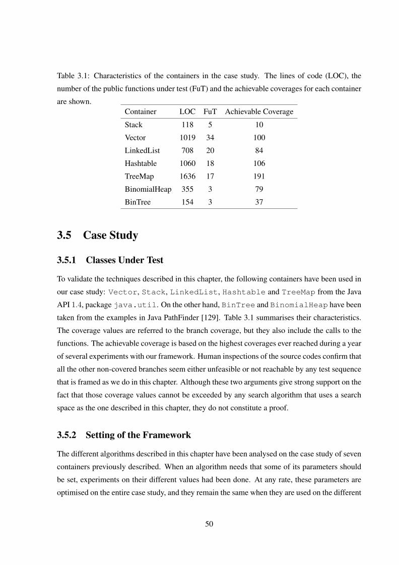
Table 3.1: Characteristics of the containers in the case study. The lines of code (LOC), the
number of the public functions under test (FuT) and the achievable coverages for each container
are shown.Container LOC FuT Achievable Coverage
Stack 118 5 10
Vector 1019 34 100
LinkedList 708 20 84
Hashtable 1060 18 106
TreeMap 1636 17 191
BinomialHeap 355 3 79
BinTree 154 3 37
3.5 Case Study
3.5.1 Classes Under Test
To validate the techniques described in this chapter, the following containers have been used in
our case study: Vector, Stack, LinkedList, Hashtable and TreeMap from the Java
API 1.4, package java.util. On the other hand, BinTree and BinomialHeap have been
taken from the examples in Java PathFinder [129]. Table 3.1 summarises their characteristics.
The coverage values are referred to the branch coverage, but they also include the calls to the
functions. The achievable coverage is based on the highest coverages ever reached during a year
of several experiments with our framework. Human inspections of the source codes confirm that
all the other non-covered branches seem either unfeasible or not reachable by any test sequence
that is framed as we do in this chapter. Although these two arguments give strong support on the
fact that those coverage values cannot be exceeded by any search algorithm that uses a search
space as the one described in this chapter, they do not constitute a proof.
3.5.2 Setting of the Framework
The different algorithms described in this chapter have been analysed on the case study of seven
containers previously described. When an algorithm needs that some of its parameters should
be set, experiments on their different values had been done. At any rate, these parameters are
optimised on the entire case study, and they remain the same when they are used on the different
50
containers. Although different tests on these values have been carried out, there is no guarantee
that the chosen values are the best.
Regarding the parameters defined in Section 3.3.2, we use J = −2, P = 58, ψ = 0.1 and
α = 1.3. RS samples sequences up to length 60. The cool rating in SA is set to 0.999, with
geometric temperature reduction and one iteration for temperature. The initial neighbourhood
size is 3. The value of α in Equation 3.16 is 0.5. The GA uses a single point crossover with
probability 0.2. Mutation probability of an individual is 0.9. Population size is 64. Rank
selection is used with a bias of 1.5. At each generation, the two individuals with highest fitness
values are directly copied to the next population without any modification (i.e., the elitism rate
is set to two individuals for generation). The MA uses a single point crossover with probability
0.9. Population size is 8. Rank selection is used with a bias of 1.5. Elitism rate is set to one
individual for generation.
3.5.3 Experiments and Discussion
Each algorithm has been stopped after evaluating 100,000 sequences. The machine used for
the experiments was a Pentium with 3.0 GHz and 1024 Mbytes of ram running Linux. The
experiments have been run under a normal usage of the CPU. Table 3.2 shows the performances
of these algorithms on 100 runs with different random seeds.
Using the same data, Mann Whitney U tests have been used to compare the median values
of the different algorithms. The performance of a search algorithm is calculated using Equa-
tion 3.2. The level of significance is set to 0.05. HC and SA are statistically equivalent on
Hashtable. HC and GA are equivalent on Stack, LinkedList and BinomialHeap.
Finally, HC and MA are equivalent on Stack, Vector, BinomialHeap and BinTree.
If we compare Table 3.2 with the highest achievable coverages (shown in Table 3.1), then
we can see that only TreeMap is difficult to test. Besides, from that table and from the sta-
tistical tests the MA seems the best algorithm. Apart from Vector, it gives the best results
on LinkedList, Hashtable, TreeMap and it is among the best algorithms on the other
containers. Moreover, the HC seems to have better performance than the GA. This is a very
interesting result, because usually local search algorithms are suggested of not being used for
generating test data [46]. Although the search spaces for software testing are usually “complex,
discontinuous, and non-linear” (J. Wegener et al. [46], 2001), the evidences of our experiments
lead us to say that it does not seem true for container classes. However, more experiments on a
larger case study and the use of different search algorithms is required.
51

Table 3.3 compares the performance of the MA when it is stopped after 10,000 and 100,000
fitness evaluations. Apart from TreeMap, MA is able to get high quality results in a very short
amount of time.
The performance of RS deserves some comments. In fact, it is sensibly worse than the per-
formances of the other algorithms. Although a reasonable coverage can be achieved, RS poorly
fails to obtain it without a long sequence of FCs. This can be explained by the fact that not only
the search landscape of the input parameters is large and complex, with only a small subset of
it that gives optimal results, but also the search space of the methods has similar characteristics.
For example, some methods need to be called few times (e.g., isEmpty) whereas others need
to be called many times (e.g., insert) to cover a particular branch. In RS the probabilities
of their occurrences in the test sequence are the same, so we will have redundant presence of
functions that need to be called only few times. Moreover, the FCs require to be put in a precise
order, and obtaining a random sub-sequence with that order might be difficult if the total length
is too short.
3.6 Limitations
The system described in this chapter is not able to generate input data for covering all the branch
statements in the source code of the CuT. This is due to different reasons:
• The framework also tries to cover the branches in the private methods. The generated
test sequences do not access directly to the private methods of the container. They can
be executed only if at least one public method can generate a chain of FCs to them. Al-
though using Java reflection a driver can directly call private methods of the CuT, besides
the fact that a driver can be located inside the CuT, it has been preferred to test directly
only the public methods. It is possible to do assumptions on the semantics of the public
methods of a container (see Section 3.3.2), but little can be said about the private ones.
Thus, the proposed space reduction techniques cannot be applied to them.
• The very few public methods with complex input parameters (11 on a total of 105
in our case study) cannot be directly called by our tool. If they are not called by other
methods, they will not be tested.
• Some methods can return objects whose class is implemented inside the same file of the
CuT or even in the same method. For example, the method keySet in TreeMap returns
52

Table 3.2: Comparison of the different search algorithms on the case study. Each algorithm has
been stopped after evaluating up to 100,000 solutions. The shown values are calculated on 100
runs of the framework. Mann Whitney U tests show that the MA has the best performance on
all the containers but Vector.Container Search Algorithms Coverage Length
Mean Variance Median Mean Variance Median
Stack Random 10.00 0.00 10.00 6.64 0.41 7.00
Hill Climbing 10.00 0.00 10.00 6.00 0.00 6.00
Simulated Annealing 10.00 0.00 10.00 6.06 0.06 6.00
Genetic Algorithm 10.00 0.00 10.00 6.00 0.00 6.00
Memetic Algorithm 10.00 0.00 10.00 6.00 0.00 6.00
Vector Random 85.21 1.52 85.00 56.99 7.73 58.00
Hill Climbing 100.00 0.00 100.00 47.67 1.05 48.00
Simulated Annealing 99.99 0.01 100.00 45.76 1.11 46.00
Genetic Algorithm 99.99 0.01 100.00 46.87 1.63 47.00
Memetic Algorithm 100.00 0.00 100.00 47.89 2.64 48.00
LinkedList Random 69.96 1.82 70.00 55.27 14.00 56.00
Hill Climbing 84.00 0.00 84.00 38.48 10.27 38.00
Simulated Annealing 82.47 2.25 82.50 33.60 5.29 33.50
Genetic Algorithm 83.83 0.26 84.00 36.66 3.64 36.00
Memetic Algorithm 84.00 0.00 84.00 36.43 3.58 36.00
Hashtable Random 92.92 1.17 93.00 54.45 25.97 56.00
Hill Climbing 106.00 0.00 106.00 35.25 0.19 35.00
Simulated Annealing 105.84 0.74 106.00 34.98 0.77 35.00
Genetic Algorithm 101.14 6.50 100.00 31.10 6.31 30.00
Memetic Algorithm 106.00 0.00 106.00 35.01 0.01 35.00
TreeMap Random 151.94 5.85 152.00 54.11 26.87 55.00
Hill Climbing 188.76 0.71 189.00 51.23 10.08 51.00
Simulated Annealing 184.19 5.75 185.00 40.68 5.88 41.00
Genetic Algorithm 185.03 3.46 185.00 42.14 8.44 42.00
Memetic Algorithm 188.86 0.65 189.00 50.55 10.31 50.00
BinomialHeap Random 77.52 0.29 77.50 47.08 100.24 47.50
Hill Climbing 77.96 0.48 78.00 24.05 34.86 25.00
Simulated Annealing 76.41 0.24 76.00 16.02 41.84 14.00
Genetic Algorithm 77.70 0.92 77.00 19.08 24.54 16.00
Memetic Algorithm 77.66 0.87 77.00 18.65 24.61 15.00
BinTree Random 37.00 0.00 37.00 26.86 15.39 27.00
Hill Climbing 37.00 0.00 37.00 9.02 0.02 9.00
Simulated Annealing 36.98 0.02 37.00 9.38 0.40 9.00
Genetic Algorithm 37.00 0.00 37.00 9.21 0.21 9.00
Memetic Algorithm 37.00 0.00 37.00 9.00 0.00 9.00
53

Table 3.3: Performance of MA on the case study.Container Fitness Average Average Time
Evaluations Coverage Length (seconds)
Stack 10k 10.00 6.00 0.29
100k 10.00 6.00 2.80
Vector 10k 99.50 73.70 8.89
100k 100.00 47.89 78.58
LinkedList 10k 83.60 50.60 2.22
100k 84.00 36.43 17.41
Hashtable 10k 105.90 36.10 1.31
100k 106.00 35.01 11.75
TreeMap 10k 184.90 47.40 3.00
100k 188.86 50.55 28.83
BinomialHeap 10k 77.30 19.10 1.87
100k 77.66 18.65 16.22
BinTree 10k 37.00 9.30 0.18
100k 37.00 9.00 1.49
54

a Set whose class is implemented inside keySet. Because our system does not call
any method on the returned objects of the tested methods, such internal classes cannot be
tested.
• For a given test sequence, only one constructor is called. One option to solve this problem
might be to use multiple sequences, each one that uses a different constructor.
• Some branches can be infeasible. This is a general problem that is not related to the used
testing tool.
3.7 Formal Theoretical Analysis
3.7.1 General Rules
The length of test sequences can have an important role in the success rate of search algorithms.
To give more general results that can be applied to any software, in this section we formally
analyse the conditions for which longer test sequences are more successful.
To simplify the analysis, we do not consider the initialisation of the object instances used
in the test sequences. Let M be the set of different methods. Each method can take as input
an element from a set I of infinite cardinality. For simplicity but without loss of generalisation,
let consider that I is equal for each method, and each method takes as input only one element.
The length of the sequence is l. Constraint for a given length on the variables are represented
by choosing a subset C(l) of inputs, i.e. C(l) ⊂ I . Let t be a test sequence for the search space
S(l), then t(k) with k ≤ l is a test sequence that consider only the first k FCs.
Let R(l) ⊂M ×C(l) be the subset of FCs that does not influence the covering of the target
branch. For example, in the case of insertion/removal of elements in a container, the call to
read-only methods like size() does not have any effect.
Let G(l) the set of global optima for the length l. The number of possible sequences is
|S(l)| = |M |l · |C(l)|l. Let r(l) be the ratio of global optima over the number of possible
solutions, i.e. r(l) = |G(l)|/|S(l)|. We can hence prove the following theorems (details are in
Appendix A.1):
Theorem 3.7.1. If R 6= , |G(l)| > 0 and |C(k)| = c (where c is a positive constant c > 1)
for all k ≥ l, then r(k + 1) > r(k) for all k ≥ l.
Theorem 3.7.2. If |G(l)| > 0 and |C(k + 1)| > |C(k)| for all k ≥ l, then it is not necessarily
true that r(k + 1) > r(k) with k ≥ l.
55
3.7.2 Discussion
These two theorems have some interesting consequences. Theorem 3.7.1 gives the conditions
for which longer test sequences are necessarily better. These conditions are very general, and
can be applied to practically most types of software. However, the price of general rules is that
they are weaker. In fact, although Theorem 3.7.1 states that longer sequences are better, without
considering the actual software (or some restricted sets) we can say only little about how much
the improvement is. At the current moment, we are not even able to state whether under the
same conditions of Theorem 3.7.1 we can have (l→∞) ⇒ (r(l) = 1) (this will be studied in
future work).
Intuitively, for longer sequences it is easy to expect more optimal solutions. But at the
same time the space of possible solutions increases as well. Theorem 3.7.1 formally proves the
non-obvious fact that their ratio increases as well.
Theorem 3.7.2 gives the conditions for which it is not necessarily true that longer sequences
are better. Note that it does not mean that they would be worse for sure. It is important to note
that this can happen when we increase the space of available inputs for longer sequences, i.e.
|C(l + 1)| > |C(l)|. This is actually the type of constraints we used in this chapter.
The choice of the input constraints is important for many automated testing techniques (e.g.,
[130, 128, 2]), but not for the ones that use symbolic execution (e.g., [129, 140]). A formal
analysis of the length of test sequences for symbolic execution based techniques will be matter
of future work.
3.8 Conclusions
This chapter has presented search based test data generation techniques for OO software, in
particular for Java containers. Search algorithms like RS, HC, SA, GAs and MAs have been
applied and compared.
The objective of minimising the length of the test sequences has been addressed as well.
Because that minimisation can be misleading, discussion on how and why a search algorithm
can be deceived has been presented, besides how to avoid it. Formal theoretical analyses on the
role of the length of test sequences have been presented as well to give more general results.
Although different settings of the parameters of the algorithms can lead to different results,
we have empirically shown that our MA performs better than the other algorithms in our case
study. Moreover, the HC resulted better than GA. This can seem strange, because local search
56

algorithms are suggested of not being used for generating test data [46]. This can happen be-
cause for the considered families of search algorithms there are several variants. Therefore, it
is not strange that a family is not necessarily better than another one for each of its variants. In
other words, it could happen that GAs are in general better than HC, but there could be variants
of GAs that are worse than some variants of HC (as it happened in our case study).
Software testing is still an open research problem. Still many research questions need to
be answered. In this chapter we hence have given the contribution of extending search based
software testing. This is important because software testing is one of main component of our
novel co-evolutionary framework that we introduce in the following Chapter 4.
57

Chapter 4
Co-evolutionary Framework
4.1 Motivation
Many software engineering activities rely on the writing and modification of source code. The
automation of these activities is highly valuable, but at the same time it is very difficult. Coding
is in fact a challenging task, which requires specialised skills.
Given a software engineering task of that type, to try to solve it we can search the space
of possible programs until we do not find one that fulfils our goal. Unfortunately, the search
space of possible programs is extremely large [23]. An exhaustive search cannot be carried out.
However, if a fitness function can be defined, then we can use search algorithms. Depending on
the nature of the fitness landscape, search algorithms could be effective even in a so extremely
large search space.
Once we define a fitness function depending on the software engineering task we want to
solve, we can use for example GP (see Section 2.4) to evolve programs rewarded by that fitness
function. However, a lot of issues arise with this approach. A more complex framework requires
to be developed to address them.
In this chapter we propose a novel framework to tackle software engineering problems that
depend on the modification and generation of source code. To use this framework, the evolving
programs need to be run on test cases. The test cases have to be either directly provided or an
automated oracle has to be available.
What we present in this chapter is a conceptual framework that needs to be instantiated
for each particular software engineering problem we want to address. In fact, each software
engineering task has its own specific properties that should be exploited. Nevertheless, all
these software engineering activities share some common issues whose way to solve them is
58

abstracted in our conceptual framework.
4.2 The Framework
We present a conceptual framework to evolve programs to solve some types of software engi-
neering problems. The framework is composed of the following components:
• Objectives for the fitness function.
• Input of the framework.
• GP engine.
• Initialisation of the genetic programs.
• Preservation of the semantics.
A more detailed description of each components follows in the next sub-sections. For each
software engineering task we want to solve, we need to instantiate and specialise some of these
components. The other components would be practically the same for each software engineering
task.
4.2.1 Fitness Function
The fitness function should tell us how good our evolving programs are in solving the software
engineering task we are addressing. Obviously, the fitness function would be specific to the
software engineering task.
There can be at least two ways in which a fitness function can be evaluated:
Statically: each program is statically checked to verify some of its properties. Static properties
could be for example either its size or the value of some specific software metrics [149].
Dynamically: each program is run against a set of test cases T . The fitness function would
be based on properties of these executions (e.g., execution time). There is the problem of
how to choose adequate test cases, and whether or not changing them during the evolution
of the genetic programs.
59

The fitness function could be composed of more than one objective Oi. In these cases, these
objectives can be linearly composed in a single fitness function f , like for example f(P ) =∑OiωiOi(P ), where P is the genetic program we are evaluating the fitness of, and ωi is a
constant weight for the objective Oi. One issue with this approach is that we need to define
weights for each objective.
A more appropriate way to deal with more than one objective at the same time is to use multi-
objective algorithms [142]. Indeed, in search based software engineering that type of algorithm
has started to be used quite often in recent years (e.g., [59, 150, 151, 152, 153, 154, 155, 156]).
Multi-objective algorithms are based on the concept of pareto dominance. A solution is dom-
inated if at least one other solution in the current population exists that is better in at least one
objective and not worse on the other objectives. A multi-objective evolutionary algorithm would
keep at each generation a set of non-dominated solutions (i.e, the pareto front). These solutions
represent the best in the population. Selection and acceptance of offspring mechanisms would
be based on these pareto relations.
Bloat [95] would easily be one of the objectives Oi to optimise.
4.2.2 Input of the Framework
The framework could take as input different things, like for example the source code of a pro-
gram (if we are trying to modify/improve it) and/or a formal specification. Specific test case
sets (or tools to produce them) could be provided as well. The type of inputs to the framework
clearly depends on the software engineering task we are trying to solve.
For example, in automatic refinement (see Chapter 5) we would have as input only a formal
specification, whereas for improvement of software (see Chapter 7) we would have the source
code of the program we want to improve but not its formal specification.
4.2.3 GP Engine
To evolve programs to solve software engineering problems we use GP. Technically, we could
use any other search based algorithm (e.g., Grammatical Evolution [157]). Our choice is based
on the fact that GP is the most used and studied paradigm to evolve programs.
GP is mainly used for machine learning applications. However, for software engineering
problems we likely would not have noise in the data. For most software engineering tasks, the
data would be test cases whose expected outputs are either automatically labelled by a formal
specification or that are manually done by human software testers. These test cases partially
60

define the semantics of the software. If even one test case is failed, this would mean that the
semantics is not satisfied. Hence, we do not need to worry of overfitting the data, we have in
fact to overfit them. If the semantics is not what it should have been, then we cannot expect that
programs that evolve based on that semantics could be able to understand that the semantics is
not correct.
For the GP engine we use in our framework, we chose the open source library ECJ [158].
It is a powerful library written in Java that supports many features of GP, like for example
strongly typed genetic programming (see Section 2.4). Many operators and characteristics of
the GP system in ECJ are inspired by Koza’s work [92], like for example single point crossover.
In that type of crossover, given two parent individuals, the offspring will be copies of their
parents with two random sub-trees from different parents that are swapped.
In literature of GP, there has been a bias toward the crossover operator. However, mutation
operators are not necessarily less useful [159]. ECJ provides six different types of GP mutation
operators. Unless stated otherwise, in our framework we use all of them. Given k a random
node in the mutating GP individual, these mutation operators are as follows:
• Point Mutation: the sub-tree rooted at k is replaced with a new random sub-tree with
bounded depth.
• OneNode Mutation: k is replaced by a random node with same constraints and arity.
• AllNodes Mutation: each node of the sub-tree of k is randomly replaced with a new node,
but with same type constraints and arity.
• Demote Mutation: a new node m is inserted between k and the parent of k. Hence, k
becomes a child of m. The other children of m will be random terminals.
• Promote Mutation: the sub-tree rooted at the parent of k will be replaced by the sub-tree
rooted in k.
• Swap Mutation: two children of k are randomly chosen. The sub-trees rooted at these two
nodes are swapped.
Bloat is one of the main problems of GP [95, 23]. However, in many software engineering
problems we would expect of not having it (or at least its negative effects would be less serious).
When the fitness function is only based on how many test cases are passed, then a program that
passes all of them would be optimal. No further improvement of the fitness would justify the
increase of the program size. In most software engineering problems, we could expect that
61

such optimal programs that solve those tasks exist. Nevertheless, we still need to use bloat
control, because the code could still substantially increase until such an optimal program would
be found. Unless otherwise stated, we use constraints on the depth of the GP trees and we use a
parsimony control (i.e., rewarding minimisation of the tree sizes) in the fitness function.
4.2.4 Initialisation of GP
In most GP applications, in the first generation all the individuals are randomly sampled, using
for example Koza’s ramped half-and-half initialisation method [92]. We are aware of only two
exceptions. Langdon [160] studied a seeding strategy based on perfect individuals. These indi-
viduals perfectly fit the training data but are not able to generalise. Westerberg used advanced
seeding strategies based on heuristics and search strategies like depth first and best first search
[161]. In both cases, these seeding strategies obtained better results than random sampling.
When in a software engineering task we need to modify an existing program P to obtain a
new version P ′, the code of this program P would be given as input to our framework. Evolving
from scratch P ′ (i.e., random seeding of first generation of GP) would likely be unfeasible if
P is a complex software. Because we can assume some relations between P and P ′, we can
exploit the source code of P to design novel seeding strategies. A simple strategy that we can
call clone strategy would be for example to have all individuals in the first generation of GP to
be exact copies of P .
When seeding strategies that exploit the source code of P are designed, there is a trade-
off between exploration and exploitation. On one hand, greedy strategies like cloning would
constrain the search in a particular area of the search space that could be sub-optimal. On the
other hand, the other extreme of having random individuals could make the evolution of P ′
too difficult. Depending on the problem, seeding strategies between these two extremes would
likely obtain better results.
4.2.5 Preservation of the Semantics
When we evolve programs to solve a software engineering task, we need to make sure that the
evolved output program is semantically correct. In most cases, even if a formal specification is
provided, we cannot prove that a program is semantically correct. However, we can use software
testing to increase our confidence in the software correctness [18].
Depending on the software engineering task and on the input to our framework, we can have
two main different types of oracle. An oracle is an entity that tells us whether for a given input
62

x the output we obtain is correct. In the best case we can have an oracle that is able to classify as
many outputs as we want. This would be the case for example if we have a formal specification
or if we an executable program P and our goal P ′ should be semantically equivalent to P (that
would be the case for example when we want to optimise non-functional criteria, see Chapter
7). In the worst case, the oracle can be used only a limited amount of times. In that case,
we would have a limited set of test cases. This would happen for example if the test cases are
manually written by human software testers. Because in general human resources are expensive,
we cannot expect of having large amounts of test cases developed in this way.
To check whether a program has faults, we can test it. This means that we run it against a
set of test cases T and then we check whether they are all passed. Apart from trivial cases, we
cannot run a program against all its possible inputs in feasible time. Therefore, software testing
cannot guarantee that a program is faultless [18]. However, the more passed tests there are the
more confidence we can have on the program correctness.
To guide GP to evolve and to maintain semantically correct individuals, we can add a se-
mantic objective to the fitness function. Given a set of test cases T produced by the given oracle,
we check how many test cases in T are failed each time we evaluate the fitness function of a
new GP individual. The objective would be to minimise this number of failed test cases.
We can have a binary score 0 for a passed test and 1 if it is failed. However, if it is possible
to have different degrees of failure, then we can exploit this information to give more gradient
to the search. For example, if the expected output is an integer y′ and the actual obtained value
is y, then we can use for example |y′ − y| instead of a binary classification passed/failed. Using
this simple heuristic, a program that gives as output the value 99 when the expected value is 100
would be better than a program that gives as output the value 0. To note that in both cases the
programs are faulty, but we just use an heuristic to state which one is more seriously faulty.
A program that is able to pass all the test cases in T is not necessarily correct. To improve
our confidence in the program correctness, it would be better to change T at each generation
of GP. Therefore, the programs will be tested on more different test cases instead of always the
same fixed ones. But how to change the test cases? This is not a trivial question, because just
getting random test cases would likely end up in worse results. This is because software testing
is a difficult task [18, 19]. Ideally, we would want to have test cases that are able to find faults
in the new evolved programs and that the current T is not able to show these faults. This means
that we are actually doing a new testing phase at each generation of GP, and we can use any
software testing technique to produce these new test cases. For example we can use a GA (see
Section 2.3.6).
63

G T
g0
g1
g2
t0
t1
t2
(a)
G T
g0
g1
g2
t0
t1
t2
(b)
G T
g0
g1
g2
t0
t1
t2
(c)
Figure 4.1: G is the population of programs, whereas T is the population of test cases. For
simplicity, sets of cardinality 3 are displayed. In picture (a) it is shown on which test cases the
fitness of the first program g0 is calculated. On the other hand, the picture (b) shows on which
programs the fitness for the first test case t0 is calculated. Note that the arc between the first
program and the first test case is used in both fitness calculations. Finally, picture (c) presents
all the possible |G| · |T | connections.
At each generation we evolve the test cases. The fitness value of a test case is based on
how many programs in the current generation of GP it is able to make fail. It is a maximisation
problem. A test case that is passed by all the programs would have the worst fitness value.
The GP individuals evolve trying to pass all the test cases, while the test cases evolve trying
to find the new faults potentially introduced in the new GP populations. This leads to a com-
petitive co-evolution like in nature happens between predators and prey. Figure 4.1 shows the
relations between the fitness functions of the programs and the test cases.
When we have an oracle that can generate only a limited set of test casesK, a co-evolutionary
algorithm can still be employed. Instead of generating new test cases, we can use K as a pool
from which a sub-set T is chosen from at each GP generation. The fitness values of the test
cases would still be employed to choose which test cases to use to create T .
To test the GP programs in a more effective way, the test cases in T should be all unique. It
would also be important to promote a certain degree of diversity among the test cases. Diversity
could be based on structural criteria (e.g., branch coverage), and it could be rewarded in the
fitness function. Because that would lead to a better testing, we could expect better final results
of our framework.
64

4.3 Strength and Limitations
The conceptual framework we present in this thesis has the strength that it could be used to
automate many different software engineering activities. It can be used in activities in which
source code needs to be automatically generated or modified. For many of these activities, their
automation has been practically absent or limited in literature.
The efficiency of search algorithms is related to the available computational resources. More
computational power means more fitness evaluations that can be done. Evaluating a larger
sample of the search space can lead to better results. On the other hand, static tools in literature
(see Chapters 5 and 6) would not be able to exploit the increasing computational power that is
available to software developers.
At any rate, our framework has the following problems and limitations:
• The fact that in the search space there is an optimal solution does not mean that a search
algorithm will find it. This mainly depends on the properties of the fitness landscape,
e.g. ruggedness and modality [162]. If for a particular software engineering problem
we cannot provide a smooth fitness function, then it is very unlikely that our framework
would find any optimal solution.
• Even with a good fitness function, the search space could be simply too large and/or
the fitness function could be too computationally expensive to calculate. Successful ap-
plications of our framework on small software could not then scale to larger real-world
software.
• Because software testing cannot guarantee the faultless of software, we would still need
that software developers would have to check the outputs of our framework. This would
be done to confirm whether the software is indeed semantically correct. Unfortunately,
the output programs from GP systems are often very difficult to read and to understand.
This is a general problem in GP. We could add a readability objective to maximise in the
fitness function, but it could harm the search process by constraining it in sub-optimal
areas.
4.4 An Example: Reverse Engineering
In this section we briefly discuss the possible application of our framework to the important
software engineering task called reverse engineering [163]. We have not carried out any empir-
65

ical study on this problem. Empirical studies on other software engineering activities follows
in the next chapters. The description given in this section is useful to help to understand how to
use our framework to other software engineering problems not discussed in this thesis.
One application of reverse engineering is that, given as input the assembler or byte-code of
a program, we want to obtain the original source code. This becomes more challenging if the
software has been compiled with the aim of making its decompilation more difficult. This could
be done for example by obfuscating the compiled code [164, 165, 166, 167].
We can use our framework to tackle this problem. The goal is to obtain a source code that,
once compiled, is equivalent to the executable we want to reverse-engineer.
The execution of the input assembler/bytecode can be used as an oracle for the test cases.
Initialising the genetic programs at random is possible, but likely it will make the search too
difficult. Therefore, smart seeding strategies that exploit the assembler code should be designed.
The fitness function is based on the semantic equivalence that is calculated on how many test
cases are passed.
GP often generate code that is difficult to understand by humans. If the obtained source
code is too difficult to understand, it would be of little help. Including a readability objective in
the fitness function is hence compulsory. At any rate, there are cases of obfuscating techniques
that make difficult to obtain even a compilable source code (e.g., [165]). In these cases, our
technique would be useful even if the evolved code would be difficult to read.
Some obfuscating techniques add complex junk code that current static tools are not able to
recognise. If we include the execution time in the fitness function, our framework could be able
to remove them. Hence, the resulting source code would be easier to understand.
The equivalence of the semantics is particularly problematic in this software engineering
activity. In fact, the user would not know the semantics of each component of the software,
hence (s)he cannot check whether the output code of our framework is valid or not. Still, the
output code generated with our framework could give important information on the nature of
the target software.
Note that there has been work on reverse engineering with search algorithms [168], but it
was not on the decompilation of code. For example, in [168] the goal was to obtain software
architectures from source code.
66

4.5 Conclusion
In this chapter we have presented a novel conceptual framework to tackle software engineering
problems that require the writing and modification of source code. The framework has been
presented at a sufficient abstract level to be applicable to different software engineering activ-
ities. Other software engineering activities not discussed in this thesis could be addressed as
well.
We analysed and discussed each component of the framework. Strength and limitations have
been outlined. An example of its application has been discussed.
To be successful, not only we need to instantiate the framework for the particular software
engineering task we want to solve, but we also need to exploit its properties. The exploitation
of domain knowledge can make possible to design more specific and tailored algorithms that
likely would produce better results.
To assess the validity of our framework, in the next three chapters we analyse in more details
its application to three different software engineering tasks.
67
Chapter 5
Automatic Refinement
5.1 Motivation
Writing a formal specification (e.g., in Z [169] or JML [170]) before implementing a program
helps to identify problems with the system requirements. The requirements might be for ex-
ample incomplete and ambiguous. Fixing these types of errors is very difficult and expensive
during the implementation phase of the software development cycle. However, writing a formal
specification might be more difficult than implementing the actual code, and that might be one
reason why formal specifications are not widely employed in industry [171].
However, if a formal specification is provided, exploiting the specification for automatic
generation of code would be better than employing software developers, because it would have
a much lower cost. Since the 1970s the goal of generating programs in an automatic way
has been sought [172]. A user would just define what he expects from the program (i.e., the
requirements), and it should be automatically generated by the computer without the help of
any programmer.
This goal has opened a field of research called Automatic Programming (also called Auto-
matic Refinement) [173]. Unfortunately, this task is much harder than expected. Transformation
methods are usually employed to address this problem (e.g., [172, 174, 175, 176, 177, 178]).
The requirements need to be written in a formal specification, and sequences of transformations
are used to transform these high-level constructs into low-level implementations. Unfortunately,
this process can rarely be automated completely, because the gap between the high-level speci-
fication and the target implementation language might be too wide.
In this chapter, we instantiate our novel conceptual framework (described in Chapter 4) to
evolve programs from their specification. To improve the performance of our framework applied
68
to this problem, in this chapter we also investigate the role of Automated N-version Program-
ming [179]. Furthermore, we exploit the formal specification to divide the set of unit tests into
sub-sets, each of them specialised in trying to find faults related to different reasons of program
failure. To evolve complex software composed of several functions, if there are relations among
the functions (e.g., an hierarchy of dependencies), then we exploit these relations. For example,
we can use them to choose the order in which the specifications of the single functions are au-
tomatically refined, and then we use the programs evolved so far to help the refinement of other
functions.
We have implemented a prototype of our conceptual framework in order to evaluate and to
analyse it. Seven different problems are used in our empirical study. The use of the formal
specifications to automatically create fitness functions makes it possible to apply the framework
to any problem that can be defined with a formal specification. However, evolving correct
programs to solve for example the halting problem [180] is not possible.
The main contribution of this chapter is a novel approach to Automatic Programming, in
particular the automatic refinement of formal specifications. This approach has a wider range of
applications than previous techniques reported in literature, because it makes no particular as-
sumption on the gap between the formal specification and the target implementation. However,
it is a very difficult task, and we obtained positive results only on small programs.
The chapter is organised as follows. Section 5.2 reviews related work. A description of how
programs can evolve to satisfy a formal specification follows in Section 5.3, whereas how to
optimise the training set is explained in Section 5.4. Section 5.5 briefly describes what N-version
Programming is and how it can be exploited to improve the performance of our framework. A
discussion on how complex software might be evolved follows in Section 5.6. The case study
used for validating our novel framework is presented in Section 5.7. Section 5.8 outlines the
limitations of automatic refinement with evolutionary techniques. Finally, Section 5.9 concludes
the chapter.
5.2 Related Work
The problem we address in this chapter, and the way we try to solve it, is similar to Evolvable
Hardware [181]. The design of electronic circuits is an important and expensive task in indus-
try. Hence, search based techniques have been used to tackle this problem in which, given a
specification of a function (for hardware that can be for example a truth table), a solution that
implements the function is sought.
69

Our framework also shares some similarities with the system for evolving secure protocols
from a formal specification [182]. A protocol is a sequence of messages, and a GA was used
to evolve it. The fitness function depends on how well the protocol satisfies its specification.
Although neither GP (see Section 2.4) nor co-evolution was used, our work shares the same
idea of formally specifying the expected behaviour (what it should be done, but without stating
how to do it) of a system (e.g., programs and protocols), and then using natural computation
techniques to find a solution that implements that system.
Another related field of research is Software Cloning, in which evolutionary techniques have
been used for automatically cloning programs by considering only their external behaviours
[183]. The external behaviour of a program can be partially represented by a set of unit tests.
In other words, programs are evolved until they are able to pass all the used unit tests. It has
been argued that this technique might be helpful for Complexity Evaluation, Software Mutants
Generation, Test Fault Tolerance and Software Development in Extreme Programming [183].
Besides the different goals, the main differences from our approach are that no formal specifi-
cation was employed and that the test case sets were fixed (i.e., they did not co-evolve with the
programs).
5.3 Evolution of the Programs
5.3.1 Basic Concepts
Given the specification of a program P , the goal is to evolve a program that satisfies it (i.e.,
we want to evolve a program that is semantically equivalent to P ). To achieve this result, GP
is employed. At each step of GP, the fitness of each program is evaluated on a finite set T of
unit tests that depends on the specification. The more unit tests a program is able to pass, the
better the fitness value it will get rewarded. This set T should be relatively small, otherwise
the computational cost of the fitness evaluation would be too high. In fact, for calculating the
fitness of a program we need to run it on each unit test in T . What can be defined as “small” or
as “big” depends on the available computational resources.
5.3.2 Training Set
The set T is different from a normal training set in machine learning. Let X be the set of all
possible inputs for P , and Y be the set of all possible outputs. A program might take as input
more than one variable, henceX is a set of all those possible combinations. The element x ∈ X
70
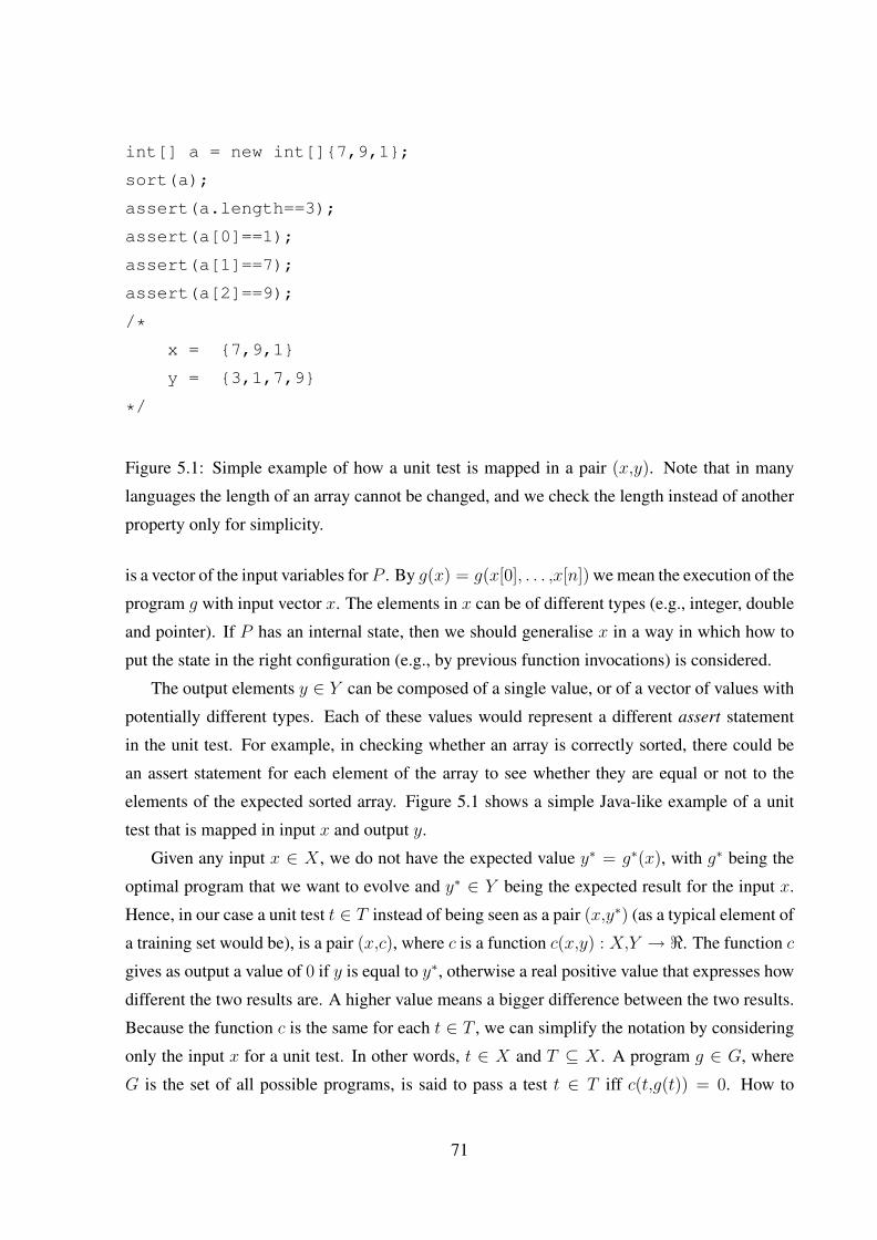
int[] a = new int[]7,9,1;
sort(a);
assert(a.length==3);
assert(a[0]==1);
assert(a[1]==7);
assert(a[2]==9);
/*
x = 7,9,1
y = 3,1,7,9
*/
Figure 5.1: Simple example of how a unit test is mapped in a pair (x,y). Note that in many
languages the length of an array cannot be changed, and we check the length instead of another
property only for simplicity.
is a vector of the input variables for P . By g(x) = g(x[0], . . . ,x[n]) we mean the execution of the
program g with input vector x. The elements in x can be of different types (e.g., integer, double
and pointer). If P has an internal state, then we should generalise x in a way in which how to
put the state in the right configuration (e.g., by previous function invocations) is considered.
The output elements y ∈ Y can be composed of a single value, or of a vector of values with
potentially different types. Each of these values would represent a different assert statement
in the unit test. For example, in checking whether an array is correctly sorted, there could be
an assert statement for each element of the array to see whether they are equal or not to the
elements of the expected sorted array. Figure 5.1 shows a simple Java-like example of a unit
test that is mapped in input x and output y.
Given any input x ∈ X , we do not have the expected value y∗ = g∗(x), with g∗ being the
optimal program that we want to evolve and y∗ ∈ Y being the expected result for the input x.
Hence, in our case a unit test t ∈ T instead of being seen as a pair (x,y∗) (as a typical element of
a training set would be), is a pair (x,c), where c is a function c(x,y) : X,Y → <. The function c
gives as output a value of 0 if y is equal to y∗, otherwise a real positive value that expresses how
different the two results are. A higher value means a bigger difference between the two results.
Because the function c is the same for each t ∈ T , we can simplify the notation by considering
only the input x for a unit test. In other words, t ∈ X and T ⊆ X . A program g ∈ G, where
G is the set of all possible programs, is said to pass a test t ∈ T iff c(t,g(t)) = 0. How to
71

<(5,-2,3), 0> // 0 represents ’not triangle’
<(4,3,6) , 1> // 1 represents ’scalene’
<(9,9,16), 2> // 2 represents ’isosceles’
<(3,3,3) , 3> // 3 represents ’equilateral’
function classifyTriangle(a, b, c)
return a + b - c;
Figure 5.2: An example of a training set for the Triangle Classification problem [18] and an
incorrect simple program that actually is able to pass all these test cases.
automatically derive the function c will be explained later in this section.
The scenario described in this chapter is very different from the normal applications of GP:
• The training set T can be automatically generated with any cardinality. There is no need
for any external entity that, for a given set of x, says which should be the corresponding
y∗.
• Usually, because there are only a limited number of pairs (x,y∗), all of them are used
for training. In our case we have the additional problem of choosing a subset T , because
using the entire X is generally not feasible.
• The training set T does not contain any noise.
• We are not looking for a program that on average performs well, but we want a program
that always gives the expected results. E.g., ∀x ∈ X • g(x) = g∗(x). Hence, a program
does not need to worry about over-fitting the training set. Even if only one test in T is
failed, that means that the specification is not satisfied.
• To prevent GP from learning some wrong patterns in the data, it would be better not
to have a fixed T . In other words, it would be better to have different test cases at each
generation. Figure 5.2 shows a non-trivial example in which an undesired pattern is learnt.
5.3.3 Heuristic based on the Specification
The function c(x,y) : X,Y → < is an heuristic that calculates how far the result y = g(t) is from
satisfying the post-condition of the specification for the input x = t when the pre-condition is
72

satisfied. If the pre-condition is not satisfied, c should return 0. Note that c does not calculate the
distance between x = t and y = g(t). It calculates the distance from y = g(t) to the expected
result y∗ = g∗(t).
It is important to note that the function c is not required to be able to compute the expected
result y∗ for an input x. Being able to state whether a particular result k is correct for an input x
(i.e., k = y∗) is enough. This can be done without knowing the value of y∗. We introduce here
an example to clarify this concept. Assume that P is a sorting algorithm that takes as input an
array of integers and sorts it. Given as input an arbitrary array x = (4,3,2,1), if the output of g
is y = (1,4,2,3), we do not need to know g∗(x) to conclude that g(x) 6= g∗(x), because y is not
sorted. We can conclude that an array is not sorted by looking at the specification of the sorting
algorithm. In this particular case, we have a 4 before a 2, which is enough to conclude that the
array is not sorted. Although a specification can state whether an array is sorted or not, it cannot
say how to sort it.
Because the expected results y∗ are not known even though a formal specification is em-
ployed, the function c cannot calculate any geometric distance between y and y∗ in the space
Y . However, because it heuristically states how far y is from satisfying the specification, a 0 as
a result means that y = y∗. Furthermore, if y 6= y∗, then c necessarily returns a value strictly
bigger than 0. Therefore, c indirectly calculates a particular type of distance between y and y∗,
although y∗ is not known.
Such a function is inspired by the one employed in Tracey’s work on Black Box Testing
[63]. In that work, the goal is to find a test case that breaks the specification. That happens in
the case of pre-condition Pr that is satisfied but the post-condition Po is not. In searching for
such a test case, the pre-condition of the function is conjugated with the negated post-condition,
i.e. W = Pr ∧ ¬Po. A test case that satisfies W does break the specification. The distance
function c is hence applied on that predicate W for guiding the search. A distance value 0 is
given if W is satisfied, and that means that a fault that breaks the specification is present for the
input t.
The main difference with our work is on what c is applied to. In this chapter we seek
a program that is correct. For guiding the search, we use this distance directly on the post-
condition when the pre-condition is true (i.e, ¬Pr ∨ Po). A distance value 0 means that the
post-condition is satisfied, so the program is correct for that particular input t. In other words,
to calculate c(t,g(t)) the program g is executed with the input data contained in the unit test
t, and then, if the pre-condition is satisfied, the result y = g(t) is compared against the post-
condition of the function to see whether the result is correct or not for that particular input
73

x = t.
How to calculate the function c? Table 5.1 is inspired by Tracey’s work [63] and shows how
to calculate a support function d, which is used to calculate how far a particular predicate θ is
from being evaluated as true. The function d takes as input a set of values I , and it evaluates the
expressions in the predicate θ based on the actual values in I . The function c is recursively built
on d, in which θ is the disjunction of the negated pre-condition with the post-condition of the
employed specification (i.e, ¬Pr ∨ Po). In other words, c is equivalent to d¬Pr∨Po. Of course,
for different specifications there will be built different functions c. The set I is hence composed
of the constants in the specification and of variables that depend on the input of c (i.e., x and y).
This type of distance d is similar to the branch distance used in white box testing (see Section
2.2).
Unfortunately, the predicates involving ∀ and ∃ can be computationally expensive if the
set of values on which they depend on is large. In our case study, these sets were arrays of
relatively small length, hence the computational cost was not so high. However, the case of
expressions like ∀x ∈ < •W (x) cannot be handled in this way. We will address this problem
in the future. One way could be to calculate the predicate on a restricted set of values, and then
evolve it at regular intervals for finding at least a value for which the predicate is false (if such
a value exists). Unfortunately, a restricted set could lead to the situation in which a predicate is
evaluated as true when it is actually false.
5.3.4 Fitness Function for the Programs
At each generation i of the evolution, the current population of genetic programs Gi is executed
on the current test set Ti. The fitness of each g ∈ Gi is based on its ability to pass the unit tests
in Ti. It is a minimisation problem, in which the heuristic function c is to be minimised over all
the test cases in Ti. If the specification is satisfied, the contribution of c to the fitness function is
equal to 0.
In evolved programs, it is easy to have code that generates exceptions, such as divisions
by zero or accessing arrays out of their bounds. In such cases, no exception is thrown by our
framework. If the GP node that generated that error is supposed to return a numerical value,
then it just returns a 0 (and hence it operates as a protected operation). However, the framework
is informed of each exception, and their number E(g,Ti) is used in the fitness function with the
aim of penalising programs that do operations that should be forbidden. The function E(g,Ti)
is calculated by counting each generated error when the program is applied on each test case in
74

Table 5.1: Example of how to apply the function d on some predicates. K can be any arbitrary
positive constant value. A and B can be any arbitrary expression, whereas a and b are the
actual values of these expressions based on the values in the input set I . W can be any arbitrary
expression.Predicate θ Function dθ(I)
A if a is TRUE then 0 else K
A = B if abs(a− b) = 0 then 0
else abs(a− b) +K
A 6= B if abs(a− b) 6= 0 then 0 else K
A < B if a− b < 0 then 0
else (a− b) +K
A ≤ B if a− b ≤ 0 then 0
else (a− b) +K
A > B dB<A(I)
A ≥ B dB≤A(I)
¬A Negation is moved inward and
propagated over A
A ∧B dA(I) + dB(I)
A ∨B min(dA(I),dB(I))
A⇒ B min(d¬A(I),dB(I))
A⇔ B min((dA(I) + dB(I)),
(d¬A(I) + d¬B(I)))
A xor B min((dA(I) + d¬B(I))),
(d¬A(I) + dB(I)))
∀x ∈ X •W if X is empty then 0 else∑v∈X dW (I[v/x])
∃x ∈ X •W if X is empty then K else
min(dW (I[v/x])) where v ∈ X
75
Ti. In GP, there is the problem of bloat. To contrast it, we penalise in the fitness function the
number of nodes N(g) of the programs. The employed fitness function f for each program g is:
f(g) =N(g)
N(g) + 1+
E(g,Ti)
E(g,Ti) + 1+∑t∈Ti
c(t,g(t)) . (5.1)
5.4 Optimisation of the Training Set
Choosing a good training set T is not easy. An ideal set T ∗ would be one that, if a program
g ∈ G passes all the unit tests t ∈ T ∗, then it is guaranteed that it will pass all the tests in
X . This means that if g completely fits the data in the training set, then it is guaranteed that g
is correct. A trivial set that satisfies such a constraint is T = X . However, the set should be
relatively small, otherwise the computational cost of fitness evaluation would be too high.
Finding the optimal T ∗ 6= X is impossible, because in the set G of all possible programs
there is always at least one program that fits all the data in this hypothetical T ∗, and can have,
for example, a special “if” statement based on the value of a t ∈ X \T ∗ that makes the program
fail on that test t. Although the use of a limited set of primitives (e.g., without “if”) might not
lead to this problem, this is not true in the general case. Even if an optimal T ∗ existed, there
is no guarantee that GP will be able to evolve a program that fits all the data in T ∗. A good
strategy for choosing an appropriate training set T is needed, because the performance of GP
depends on it. We use co-evolution to find T (see Chapter 4).
When co-evolution is employed, each t ∈ Ti has a fitness value as well. A fitness function
is used to reward unit tests that the programs in the current population Gi have difficulties in
passing. In contrast to Equation 5.1, this is a maximisation problem. A value of 0 means that
all the programs in Gi pass the test t. The fitness function is:
f(t) =∑g∈Gi
c(t,g(t)) . (5.2)
It is important to outline that the employed c(t,g(t)) values are the same as those used for
Equation 5.1. Hence, they are calculated only once, and then they are used for both fitness
functions.
Once the fitness function is calculated for each test in Ti, we use search algorithms to sample
the new test cases [19]. In particular, we employ GAs (see Section 2.3.6) to evolve the next test
set Ti+1.
However, we cannot expect to have good (in the sense of being able of finding faults) unit
tests already in the first generations of a GA. In that case, trying to evolve programs on simple
76

unit tests for many generations would not be very appropriate. Moreover, when the programs
are able to pass all the unit tests in the current generation, time would be needed to evolve more
challenging test cases.
One solution is to allow more generations for the evolution of the unit tests. For example,
every k generations of the co-evolution, a special intensive evolution of the unit tests can be
done. During such intensive evolution phases, no program evolves (and that helps to reduce
the computational overhead of the intensive evolution). Moreover, for fitness evaluation of the
unit tests, we can just use the best current program (and that helps as well in reducing the
overhead). In fact, because we do not need to evolve all programs, there is no need to execute
all of them on the unit test population (that would have been done if we needed to calculate their
fitness values), because the best program is already an appropriate candidate for evaluating the
quality of the unit tests. The pseudo-code of the algorithm used to choose test cases at each GP
generation is:
1. Evolve the GP population for one generation.
2. Calculate fitness values for each test case t ∈ Ti based on the GP programs.
3. Based on these fitness values, use a search algorithm to generate new test cases for Ti+1.
4. If current generation i is chosen for intensive evolution, then:
(a) Calculate fitness value for each test case t ∈ Ti+1 based only on the best (i.e., highest
fitness value) GP program in the current GP population.
(b) Use a search algorithm to generate new test cases and replace the old ones in Ti+1.
(c) If the termination criterion for the intensive evolution is not satisfied, go back to
point 4.a.
5. If the termination criterion is not satisfied, go back to point 1.
5.4.1 Specialised Sub-Populations
In this section we describe a co-evolutionary algorithm that is built on Tracey’s work on Black
Box Testing [184]. We call this algorithm Specialised Sub-Populations (SSP). The aims of this
algorithm are to provide more challenging test cases and to increase diversity among them.
The pre-condition of the function is conjugated with the negated post-condition. Then,
this predicate is transformed to a disjunctive normal form. For each disjunction element, an
77

independent sub-population Sj,i in Ti is used, where⋃Sj,i ⊆ Ti = Ti. In other words, the
test set Ti is partitioned into non-overlapping sets Sj,i. Each subset uses a different heuristic
function for evaluating its test cases, and the resulted fitness function to minimise depends
on the disjunction element related to the subset. For example, if the pre-condition Pr of the
program is true and the post-condition Po is A ∧ B, then it will be Pr ∧ ¬Po = ¬A ∨ ¬B.
Hence, Ti will be divided into two independent sub-populations, one that exploits d¬A(I) for
the its fitness function, and the other that uses d¬B(I).
The original idea [184] was to evolve a different unit test for each possible reason for which
the program can break the specification. It is a minimisation problem, where a value of 0 is the
optimum and it means that the considered program is failed on that particular test. However,
this is insufficient for our problem. We not only want to evolve a test population that the current
population of programs is not able to pass, but we also want it as hard as possible. Hence, we
need to exploit the function d to reward the unit tests that make the post-condition as far as
possible from being evaluated as true. Thus, we have to transform the minimisation problem
(that does not give any more information once a test is failed) to a maximisation one.
Given W a component of the disjunction we want to satisfy, the goal is to get a test case t
that maximises:
hW (t,g(t)) =
k + d¬W (I) if W is true ,
k1+dW (I)
otherwise ,(5.3)
where k is any arbitrary constant (e.g., k = 1), and the set value I is based on the variables
in t, g(t) and the constants in W . The function hW (t,g(t)) is never less than 0, and, for each
different sub-population, it can replace c(t,g(t)) in the fitness function in Equation 5.2.
The use of hW (t,g(t)) also solves another important problem. If a test is passed by all the
programs, by using only c we will get a fitness value of 0, that gives no gradient information
until at least one program that fails the test case is evolved. On the other hand, h could give
gradient information even when a test is passed.
The next sub-populations for Ti+1 are still generated with a search algorithm (i.e., GAs).
However, there is no communication among the sub-populations.
5.5 N-version Programming
After applying our framework, we get as output a program that hopefully satisfies the wanted
formal specification. However, testing cannot prove the correctness of a program, hence our
78

output program might contain faults. Therefore, in this section we discuss how we can further
improve the reliability of the programs.
Fault tolerance is the ability of software of being able to correctly behave even in the cases
in which faults occur. One technique to achieve this goal is N-version Programming [185].
Briefly, the idea is to implement the same software in several independent versions (at least 2),
and then to use all of them in parallel for the computation. The result will be chosen by a simple
voting criterion among the different versions.
If the software versions are independent (e.g, implemented by different software developers
without any communication between them), it is possible that a fault in one version will be
hidden by the other versions. However, true independence can be hard to achieve in practice.
There might be other ideas in hardware fault tolerance [186] that we could borrow in our future
work.
One problem with N-version programming is that it is expensive. The same software needs
to be implemented many times in independent ways. Hence, work on how to automate N-
version programming with GP has been proposed [179].
It is useful to note that N-version programming is conceptually the same idea as ensembles
in machine learning. An example of GP ensemble is the work of Imamura et al. [187]. N-
version programming can be used in our framework to improve its performance. For the same
software specification, different runs of the framework can be done (e.g., with different random
seeds and/or different parameter setting). Hence, the final output programs of each run can be
put together in an ensemble, although different versions in this case would not be independent
of each other.
Let S be a system that can generate a correct program p∗ from a formal specification with
probability C(S) = δ. The program p∗ will always give the right answer for all the inputs with
probability δ. The programs generated with probability 1−δ give a wrong output at least for one
input (but no assumption on the input is made, e.g., whether for each different incorrect program
these inputs are either dependent or not). Let EnS be an ensemble of n programs generated with
S. It follows that:
C(S) > 0.5⇒ limn→∞
C(EnS) = 1 , (5.4)
assuming that these n programs are independent of each other.
If δ ≤ 0.5, then it is still possible that the probability of having a correct ensemble increases.
What happens in these other cases is directly dependent on whether the faults in the programs
generated by S are independent or not. If they are independent, the faults can be covered. In
fact, even if with a low C(S), a high C(EnS) might still be obtained.
79

5.6 Evolving Complex Software
The framework described so far can be used to evolve single functions. However, unless soft-
ware is developed in a monolithic way, there are several functions that interact and depend on
each other. In this section we describe a possible way to enable our framework to deal with
these cases. Although software architectures can be very complex, we describe a simple ap-
proach here to illustrate how our conceptual framework can cope with complex software.
Let us call Z the set of function specifications of the software we want to automatically
implement. We could use our framework directly on each z ∈ Z, but that would not take into
account the dependencies among the functions. For example, let’s say that a method A needs to
call a method B. If we first evolve B, then we can use it when we try to evolve A. However, if
we try to evolve directly A that would be more difficult, because for each position in which B
needs to be called inside A we need to evolve a separate copy of B. Moreover, B can be seen
as a sub-problem of A, and the specification of B is very useful for the fitness function of A.
If we do not exploit this specification, the fitness function generated by A might give no direct
indication on how to solve this sub-problem. We can use the following simple strategy to tackle
this problem:
1. Choose a function specification z from Z.
2. Use our framework to evolve an implementation of z. If that is successful, then remove z
from Z, and add its implementation to the set of used primitives.
3. If Z 6= , then go to point 1, otherwise the algorithm terminates.
The choice of z from Z might be guided from architectural information of the system we
want to implement. For example, simple functions would be preferred to functions that depend
on some others. Hence, we would start to consider these more complex functions only when
the functions they rely on are already been evolved by the system. If a function is “considered”
correctly evolved, it will be added to the set of GP primitives. Hence, the other functions that
will be evolved afterwards will be able to use it.
If the framework is not able to evolve a particular function, it will try do it again later on
(i.e., it is not removed from Z). In fact, that function might need some other functions that
have not been evolved yet. One possible implementation of Z could be a queue that has been
ordered by exploiting the function dependencies. Therefore, if a specification z is not correctly
implemented, then it will be pushed back at the end of the queue.
80

Another optimisation could be that, instead of adding an evolved function to the general set
of GP primitives, only the functions that could need it would have it added to their set of used
primitives. However, this type of dependence is not always known.
Once all the functions have been evolved, the final complete implementation of the software
is given as output of our framework.
5.7 Case Study
In this section a set of GP primitives that defines a simple programming language is presented.
Then, seven different problems that use this set are described: MaxValue, AllEqual, Triangle-
Classification, Swap, Order, Sorting and Median. Different types of experiments are discussed
and their results are shown. Finally, comments on the results are given.
5.7.1 Primitives
In the following, we give details of a set of primitives that defines a non-trivial programming
language. It is important to note that the set was chosen without any particular bias towards the
programs in our case study. Extending our prototype to support an entire real-world language
(e.g., C and Java) is an interesting and important goal that we are currently pursuing.
Each node in our GP engine has a type, and constraints exist on which types of children a
node can have. Our language considers three types: statement, integer and boolean. The root
node of a tree should be of statement type.
The name of the primitives is consistent with their semantics. On one hand, with x and y we
represent sub-trees of integer type. On the other hand, a and b are boolean type sub-trees, and
w and z are statement sub-trees. Based on the context, we use the same symbol for representing
either a sub-tree or its output. The primitives are:
Constants: five integer constants with value from 0 to 4. Two boolean constants: true and
false.
Arithmetic Functions: (add x y), (sub x y), (mul x y) and (div x y).
Boolean Functions: (bigger x y), (bigger or equal x y), (equal x y), (and a b), (or a b) and
(neg a).
Base Statements: (skip) is the empty statement, that does nothing when executed. The con-
catenation of statement executions is done with (seq w z), whereas conditional statements
81

are done with (if a w z). In that case, w is executed only if a is true, otherwise z will be
executed. Finally, for loops we use (loop x y w), in which w is executed y-x times, and
index is an integer terminal (i.e., a leaf node) that gives either the value of the iterator
variable of the closest loop or zero if it is used outside a loop.
Variable: for simplicity, only one variable called result is supported in the language, with a
statement (write result x) and an integer terminal read result to manipulate it. If the
program that is tried to be evolved should return an integer value, then the value inside
result at the end of the computation will be given as output. Otherwise, result can be just
used as a variable for temporally storing computed data.
Integer Inputs: for any integer variable as input to the program, a terminal input i is included
to the set of primitives, where i is a constant that is different for each input variable.
Array Input: if the program takes as input an array, the primitives to handle it will be added
to the used set. We use (array x) to get the value in position x, whereas (write array x y)
writes y in position x. Finally, the terminal length returns the length of the array. Note
that only one array as input is supported.
5.7.2 Programs to Evolve
To evaluate our novel framework, seven different problems have been chosen. Some of them
take as input an array A of integers. The array is passed by reference. The length of A is
represented by l. The state of the array A after a function is executed is represented by A′.
Comparisons between arrays (e.g., A′ = A) are not on the pointers, but on the status of those
arrays (i.e., length and internal elements).
Each program has a global variable named result. All the problems described in the fol-
lowing use the same set of primitives that were described in the previous section, with some
differences based on the type of input. For each problem a specification is presented. Instead of
using a specific language like Z [169] or JML[170], we prefer to use a simple first order logic
specification for the short examples that we present. In fact, in this chapter we are presenting a
conceptual framework that could be applied to any formal specification. Hence, the choice of
a specification language is not essential. We believe that a first order logic could be more eas-
ily understood by readers not familiar with real-world specification languages (e.g., Z [169]).
Nevertheless, although the following specifications could be re-written in another language, the
derived fitness functions would be the same. Therefore, the final results would not change.
82

Extending our framework to support a specific language would just require to implement the
tool to derive the fitness function. A good fitness function would be able to give gradient in the
cases in which the specification is not satisfied. Possible problems related only to a particular
language are not addressed in this chapter.
In the following, Pr and Po are the abbreviations for pre-condition and post-condition re-
spectively.
The first program we consider is to find the max value inside A. Such a value has to be
stored in result. The specification of this problem MaxValue is shown in Figure 5.3.
In the AllEqual problem, given A as input, we want to evolve a program that is able to
say whether all the elements in A are equal to each other or not. If they are not all equal, the
variable result should store the value 0. Otherwise, it should store any value different from 0.
The specification is shown in Figure 5.4.
A very famous program in software testing is TriangleClassification [18]. Given three in-
tegers as input, the program should classify whether they represent the edge of an incorrect
triangle (in that case the program should return for example a 1), a scalene triangle (return value
2), a isosceles one (return value 3) or an equilateral triangle (return value 4). The specification
is shown in Figure 5.5.
The program Swap takes as input an array and two indexes. The values at those positions are
then swapped (Figure 5.6). Similar to Swap, the program Order swaps the two indexed values,
but only if the value in position i is bigger than the value in position j (Figure 5.7).
The Sorting problem has been widely studied in computer science [180]. Given an array as
input, the program should order the elements in the array such that the values in each position
should be equal or lower to the following elements (Figure 5.8). Although the evolution of a
Sorting algorithm has already been attempted in the past (e.g., [188, 189]), those works were
specialised in this task. In their cases, they used biased primitives and ad hoc fitness functions.
In contrast, our framework is general, and does not make any particular assumption on the
program that will be evolved. Moreover, in the case of sorting algorithms, to our best knowledge
the problem of automatically choosing the most appropriate training set has not been addressed
in literature.
Finally, we consider the problem of evolving a Median program. The specification is shown
in Figure 5.9. Modifying the array given as input does not break that specification. We could
have added A′ = A to that specification, but this would have significantly increased the com-
plexity of the possible solutions.
By using our set of primitives, possible implementations for the different specifications are
83

int MaxV alue(int[] A)
Pr : l ≥ 1
Po : ∀i ∈ [0,l − 1] • result ≥ A[i] ∧∃i ∈ [0,l − 1] • result = A[i] ∧ A′ = A
Figure 5.3: Formal specification for MaxValue.
int AllEqual(int[] A)
Pr : l ≥ 1
Po : ((result = 0 ∧ ∃i ∈ [0,l − 2] • A[i] 6= A[i+ 1]) ∨(result 6= 0 ∧ ∀i ∈ [0,l − 2] • A[i] = A[i+ 1])) ∧ A′ = A
Figure 5.4: Formal specification for AllEqual.
shown in Appendix A.2 in Figures from A.1 to A.7. To our best knowledge, the specifica-
tions for Sorting and Median algorithms that we provide cannot be refined at the moment using
transformation techniques.
5.7.3 Experiments
We first describe how the conceptual framework has been implemented, then we discuss its
parameters and how we set them. Experiments in which we compare random testing versus
co-evolution and versus co-evolution with SSP follow. The performance of the testing engine
is also shown. We then used the best configuration to carry out experiments with N-version
programming.
In our framework there is a very large number of parameters that need to be set. Trying
to optimise all of them was not possible. Hence, we chose settings that are common in the
literature, and then we did several experiments to tune the ones that we think are the most
important. The following settings are what we finally chose. However, no guarantee on their
optimality can be given. All the settings are the same for all experiments. Note that we only
show the most important settings.
We used a population size of 5000 individuals that are evolved for 200 generations. The
maximum depth allowed for a tree is 12. For generating the next population, pairs of parents
are chosen for reproduction. A tournament selection with size 7 is employed. In other words,
for choosing each parent, 7 individuals are randomly taken from the population, and the best
among them is chosen as the parent.
84

int TriangleClassification(int a, int b, int c)
Pr : true
Po : NT ∨ (V ∧ SC) ∨ (V ∧ IS) ∨ (V ∧ EQ)
NT : (a ≥ b+ c ∨ b ≥ a+ c ∨ c ≥ a+ b) ∧ result = 1
V : a < b+ c ∧ b < a+ c ∧ c < a+ b
SC : a 6= b ∧ b 6= c ∧ a 6= c ∧ result = 2
IS : ((a = b ∧ b 6= c) ∨ (a = c ∧ b 6= a) ∨ (b = c ∧ a 6= b)) ∧ result = 3
EQ : a = b ∧ b = c ∧ result = 4
Figure 5.5: Formal specification for TriangleClassification.
int Swap(int[] A, int i, int j)
Pr : A 6= null ∧ i ≥ 0 ∧ i < A.l ∧ j ≥ 0 ∧ j < A.l
Po : (∀x ∈ [0,l − 1] • (x 6= i ∧ x 6= j)⇒ A′[x] = A[x]) ∧A′.l = A.l ∧ A′[i] = A[j] ∧ A′[j] = A[i]
Figure 5.6: Formal specification for Swap.
int Order(int[] A, int i, int j)
Pr : A 6= null ∧ i ≥ 0 ∧ i < A.l ∧ j ≥ 0 ∧ j < A.l
Po : (∀x ∈ [0,l − 1] • (x 6= i ∧ x 6= j)⇒ A′[x] = A[x]) ∧A′.l = A.l ∧ ((A[i] > A[j] ∧ A′[i] = A[j] ∧ A′[j] = A[i]) ∨(A[i] ≤ A[j] ∧ A′[i] = A[i] ∧ A′[j] = A[j]))
Figure 5.7: Formal specification for Order.
int Sorting(int[] A)
Pr : true
Po : ∀i ∈ [0,l − 2] • A′[i] ≤ A′[i+ 1] ∧ A′.l = A.l ∧∀i ∈ [0,A′.l − 1] • ∃t ∈ [0,A.l − 1] • (A′[i] = A[t] ∧|j ∈ [0,A.l − 1]|A′[i] = A[j]| = |j ∈ [0,A′.l − 1]|A′[j] = A[t]|)
Figure 5.8: Formal specification for Sorting.
85

int Median(int[] A)
Pr : l ≥ 1
Po : (∀x ∈ A • (L(x) ≥ d(A.l/2)e ∧ G(x) ≥ d(A.l/2)e)⇒ result ≤ x) ∧L(result) ≥ d(A.l/2)e ∧ G(result) ≥ d(A.l/2)e ∧∃x ∈ A • result = x
L(x) : |t ∈ A|t ≤ x|G(x) : |t ∈ A|t ≥ x|
Figure 5.9: Formal specification for Median.
For each pair of parents, one of the following actions is taken for generating two new off-
spring:
• With probability 0.1, the selected individuals are directly copied into the next generation
without any modification.
• Crossover is done with probability 0.3.
• Mutation is done with probability 0.6.
Crossover takes as input two parents, and it randomly chooses one node in each of them.
The offspring are copies of the parents with the sub-trees rooted at those two nodes swapped.
Mutation operators are the ones described in Section 4.2.3.
At each generation, the best individual is copied to the next generation without any modifi-
cation, i.e., elitism rate is set to 1 individual. All the other settings that are not listed here are
used with their default values in ECJ.
To prevent the execution of very expensive programs, each program is stopped after execut-
ing at most 20 loop iterations. However, if the program takes as input an array, the allowed loop
iterations will be increased to l2 + 1, where l is the length of the array given as input. A more
appropriate automatic way to choose that limit will be studied in our future work.
To choose the test cases for Ti, we report experiments with three different techniques: ran-
dom sampling, co-evolution and co-evolution with SSP. Note that in all of these algorithms we
enforce the constraint that all the test cases in Ti should be unique. This is done because there
would be no particular benefit in testing a program on the same input more than once at each
generation.
When random sampling is employed, for each Ti we sample random test cases until we
get 100 that are different. Sampling random test cases is not straightforward. We need to
86

put constraints on the size and range of the input variables. For example, sampling extremely
long input arrays would make the testing phase too long. Hence, we decided that the length
of the arrays is randomly chosen with 16 as the maximum length. Values inside an array A
are randomly constrained in either [−128,127] or in [−l,l], and integer inputs take values in
[−128,127]. Although constraining the variables is a common technique in software testing, the
choice of these constraints is fairly arbitrary, and it might happen that faults could be discovered
only with values outside those fixed ranges. More detailed analysis is needed in future work.
When co-evolution is employed, the size of each Ti is 60, and the archive has size 40. To
evolve Ti+1 from Ti a simple GA is used. The chromosome is represented by a list of the integer
inputs (if any) of the program, and the input array (if any).
A single point crossover is applied with probability 0.75. It is used separately on the list on
integer inputs and on the input array. In other words, two different crossovers are employed,
one that combines the lists of integer inputs, the other that combines the arrays. In the case of
the input array, if the two parent arrays have different lengths, the offspring will have a length
that is the average of them.
The integer inputs are mutated with probability 1/n, where n is the number of integer inputs.
In the same way, each element in the array has probability 1/l of being mutated, where l is the
length of the array. A mutation consists of adding a discretised Gaussian noise (mean 0 and
variance 1).
Rank selection [88] is used with a bias of 1.5. Elitism rate is set to 1 individual for genera-
tion. At each new generation, a completely new individual is added to the population to prevent
that the length of the arrays degenerates to a particular low value (e.g., 0). Doing that was easier
than defining a new mutation operator that increases/decreases the length of arrays. Moreover,
in this way we do not need to handle the problem of a computationally expensive growth of
those lengths.
When random sampling is not employed, we also use a special intensive evolution of the
training set for every 5 steps of the co-evolution. In such cases, the best program gbi in Gi is
chosen and used to evolve the unit tests in Ti. In other words, the tests in Ti evolve using gbito calculate their fitness values, but no program evolves at this time. The next test set Ti+1
for the programs is evolved in such a way after 1024 generations are allowed to evolve Ti. It is
important to note that the number of these generations is lower than the size of the populationGi.
Hence, because only one program (gbi in particular) is used for the fitness function calculations,
the computational cost of this special evolution should be cheaper than the cost of one step of the
co-evolution (given the reasonable assumption that the cost of evaluating the fitness function is
87

Table 5.2: Configurations in which extra functions were added to the base set of GP primitives.
These functions are correct implementations of the specifications we address in our case study.Configurations Added primitives
Order 2 Swap
Sorting 2 Swap
Sorting 3 Order
Median 2 Swap
Median 3 Order
Median 4 Sorting
what contributes most to the total computational cost). However, if no speciation [190] is used,
the test case population can easily converge to very similar individuals. Although they might
be high fitness individuals, the loss of diversity in the test case population might decrease the
performance of the evolution of the programs.
Based on the idea presented in Section 5.6, for different specifications we also considered
variants of the primitive set. In other words, we add to it some of the already evolved programs.
We use numbers for identifying the different versions, e.g., foo i means that specification of the
program foo is evolved with a new enlarged set of primitives of index i. Number 1 uses the
basic primitive set. Table 5.2 shows these configurations.
For each program specification and GP primitive configuration (i.e., a total of 13 program
versions), we ran our framework with three different ways of selecting the test cases: random
sampling, co-evolution, and co-evolution with SSP. Each of these 39 configurations has been
run 100 times with different random seeds. All the following data presented in the different
tables were collected from these 3,900 experiments.
Table 5.3 shows how many times, out of 100, it was possible to evolve a correct implemen-
tation. To see whether there is any statistically significant difference between the performance
of random sampling, co-evolution and SSP, we also carried out statistical tests to compare these
three algorithms on each program version. The performance of such algorithms can be described
as a binomial random variable, representing whether a correct program can be evolved (value 1)
or not (value 0). To calculate whether there is any difference among the three random variables,
we used a two-tailed Fisher’s Exact Test with a 0.05 significance level on the results for each
of the 13 program versions. A p-value lower than 0.05 means that the 2 random variables are
statistically different (for that significance level).
88

To assess whether a program is correct, for each specification we have manually designed
and tailored large sets T k of 10,000 test cases each. Because no test can prove the correctness
of a program, we also manually inspected the code of the programs that are able to pass all the
tests in T k. Although this two combined actions (intensive testing and inspection) give strong
support to state whether a program might be correct, they do not constitute a proof. However,
for sake of simplicity, we will use the term correct although we do it inappropriately.
The population of test cases at the last generation can give feedback on the quality of the
testing engine. If the best program in the last generation z is able to pass all the tests in Tz,
we call it valid. If a program is correct, then it is necessarily also valid. The opposite is of
course not necessarily true. If a valid program is incorrect, this would show a poor quality of
the testing component of our framework. Table 5.4 shows the number of times in which an
incorrect program was not recognised by our framework (i.e., the number of valid programs
that are not correct out of 100 runs for each program version).
Finally, we investigated the use of N-version programming. For each program version,
we built ensembles of size up to 10. We did it by randomly picking up the best programs
in the final generation from the 100 runs. For each program version and ensemble size, we
repeat this ensemble creation 100 times with different random seeds, and we check whether
the ensembles are valid and correct. Results are presented in Table 5.5, whereas Table 5.6
presents the same type of experiment, but with the programs that are picked up only if they are
valid. For generating the test cases, we used co-evolution with SSP. We do not show the same
type of experiment with the other configurations because the results are very similar. Two-
tailed Fisher’s Exact Tests with a 0.05 significance level were carried out to state whether using
ensembles gives different performance compared to using only a single program.
5.7.4 Discussion
Table 5.3 shows that the formal specifications in our case study can be automatically imple-
mented by our framework. In fact, for all the formal specifications it was possible to evolve
a correct program at least once out of 100 independent runs of the framework. However, for
some configurations (4 out of 13) of the used primitives it was not possible to evolve a correct
program (i.e., Order 1, Sorting 1, Median 1 and Median 2).
Regarding the comparison of the three different algorithms for generating the test cases,
the results in Table 5.3 show that SSP has statistically better performance in two problems
(TriangleClassification and Order 2), but worse in one (Sorting 3). However, in this latter case
89
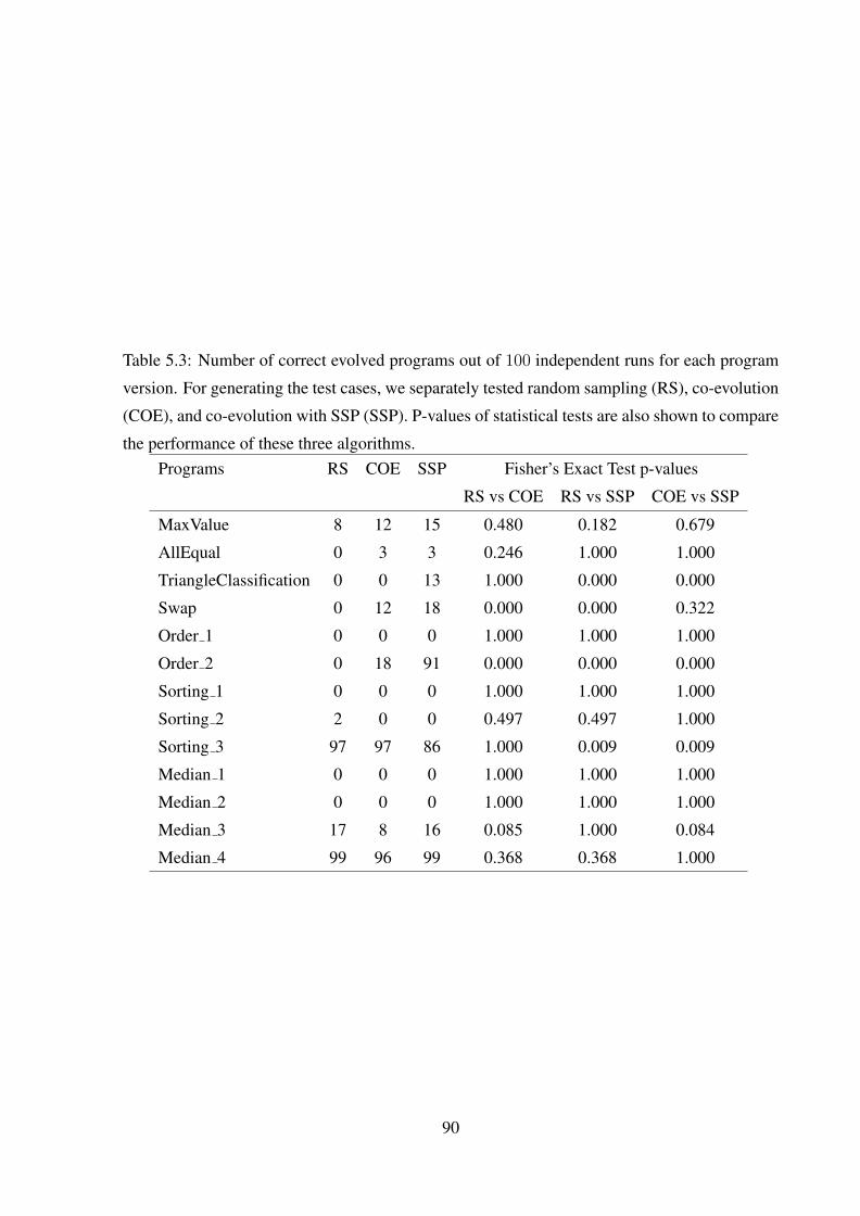
Table 5.3: Number of correct evolved programs out of 100 independent runs for each program
version. For generating the test cases, we separately tested random sampling (RS), co-evolution
(COE), and co-evolution with SSP (SSP). P-values of statistical tests are also shown to compare
the performance of these three algorithms.Programs RS COE SSP Fisher’s Exact Test p-values
RS vs COE RS vs SSP COE vs SSP
MaxValue 8 12 15 0.480 0.182 0.679
AllEqual 0 3 3 0.246 1.000 1.000
TriangleClassification 0 0 13 1.000 0.000 0.000
Swap 0 12 18 0.000 0.000 0.322
Order 1 0 0 0 1.000 1.000 1.000
Order 2 0 18 91 0.000 0.000 0.000
Sorting 1 0 0 0 1.000 1.000 1.000
Sorting 2 2 0 0 0.497 0.497 1.000
Sorting 3 97 97 86 1.000 0.009 0.009
Median 1 0 0 0 1.000 1.000 1.000
Median 2 0 0 0 1.000 1.000 1.000
Median 3 17 8 16 0.085 1.000 0.084
Median 4 99 96 99 0.368 0.368 1.000
90

Table 5.4: For each tested configuration (13 program versions for 3 algorithms), it is shown the
number of valid programs that are not correct out of 100 independent runs of the framework.
The algorithms are: random sampling (RS), co-evolution (COE), and co-evolution with SSP
(SSP).Programs RS COE SSP
MaxValue 0 0 0
AllEqual 34 78 71
TriangleClassification 0 72 36
Swap 85 1 0
Order 1 94 0 0
Order 2 94 66 7
Sorting 1 0 0 0
Sorting 2 0 0 0
Sorting 3 2 1 6
Median 1 0 0 0
Median 2 0 0 0
Median 3 31 11 30
Median 4 0 4 1
91

Table 5.5: For each program version, it is shown the number of correct evolved ensembles out
of 100 independent ensemble creation processes. The percents of correct programs in the pools
used for generating the ensembles are shown. Ensemble sizes span from 2 to 10. Both valid and
invalid programs were used for generating the ensembles.Programs Correct % Correct Ensemble
s2 s3 s4 s5 s6 s7 s8 s9 s10
MaxValue 15% 2 10 3 2 0 0 1 0 0
AllEqual 3% 0 0 2 0 0 0 0 0 0
TriangleClassification 13% 2 14 4 11 6 13 7 17 11
Swap 18% 6 11 8 6 4 5 7 6 9
Order 1 0% 0 0 0 0 0 0 0 0 0
Order 2 91% 81 98 95 100 99 100 100 100 100
Sorting 1 0% 0 0 0 0 0 0 0 0 0
Sorting 2 0% 0 0 0 0 0 0 0 0 0
Sorting 3 86% 77 94 95 99 98 100 100 100 100
Median 1 0% 0 0 0 0 0 0 0 0 0
Median 2 0% 0 0 0 0 0 0 0 0 0
Median 3 16% 1 6 3 6 4 6 7 6 5
Median 4 99% 95 100 100 100 100 100 100 100 100
92

Table 5.6: For each program version, it is shown the number of correct evolved ensembles out
of 100 independent ensemble creation processes. The percents of correct programs in the pools
used for generating the ensembles are shown. Ensemble sizes span from 2 to 10. Only valid
programs were used for generating the ensembles.Programs Correct % Correct Ensemble
2 3 4 5 6 7 8 9 10
MaxValue 100% 100 100 100 100 100 100 100 100 100
AllEqual 4% 0 4 2 1 0 0 1 1 0
TriangleClassification 27% 6 30 15 30 26 54 32 53 46
Swap 100% 100 100 100 100 100 100 100 100 100
Order 1 0% 0 0 0 0 0 0 0 0 0
Order 2 93% 92 100 97 98 100 100 100 100 100
Sorting 1 0% 0 0 0 0 0 0 0 0 0
Sorting 2 0% 0 0 0 0 0 0 0 0 0
Sorting 3 93% 90 98 99 100 100 100 100 100 100
Median 1 0% 0 0 0 0 0 0 0 0 0
Median 2 0% 0 0 0 0 0 0 0 0 0
Median 3 35% 12 26 25 21 26 34 39 45 46
Median 4 99% 99 100 100 100 100 100 100 100 100
93

it is still able to achieve a good performance of 86%. This leads us to consider SSP as the best
algorithm among the ones we analysed.
Unfortunately, the performances in general are not very satisfactory (only in 3 cases out of
13 the performance was higher than 50%). The main reason seems to be the presence of large
regions of the search space with gradient toward local optima, where a small program perfectly
satisfies a single predicate of the specification but not the others. For example, in the case of
Sorting, an empty program p1 (i.e., a program that does not do any computation) would perfectly
satisfy the constraint that the output array should be a permutation of the input one. In the same
way, a program p2, that in a single loop writes the same constant in each position of the array,
would satisfy the constraint that each element should be less than or equal to the next ones. Of
course, in this latter case the output array would not be a permutation of the input one.
Mutation operators do not seem to be suitable for escaping from the basin of attraction of
local optima in our experiments. In this example, neighbourhood solutions (i.e., solutions with
very similar tree structures) around p1 and p2 would fail both predicates (unless of course they
are semantically equivalent to either p1 or p2). Effective crossover requires the presence of
building blocks [29]. There should be blocks of the genome that would positively contribute to
the fitness value even if they are present in non-optimal individuals. Crossover can be used to
gather these building blocks and to spread them in the next generations (a detailed description
of the building blocks theory is outside the scope of this chapter, please see for example [29]
for more details). Unfortunately, neither p1 nor p2 contains any important building block, hence
an offspring generated by a crossover of p1 and p2 is likely to have a worse fitness value. De-
pending on the weights that the two predicates have in the fitness function, most of the time the
population quickly converges to either p1 or p2, and our experiments confirmed it.
Simply increasing the population size and the number of generations would not particularly
help to address the above problem. In fact, it is the fitness function that plays the main role
in this problem. A way to address it would be to formulate the function c (defined in Section
5.3.3) as a multi-objective function [142], in which each predicate is a separate objective. By
doing that, solutions that partially satisfy more than one predicate (and hence they are likely to
have some good building blocks in them) will not be disadvantaged against very small simple
programs that completely satisfy a single predicate but behave poorly on the other predicates.
For three program configurations (i.e., Order 2, Sorting 3 and Median 4) the performance
was strangely high (> 90%) compared to the other ten configurations (with the highest perfor-
mance of 18% for Swap). This means that the fitness function that is automatically derived for
those problems was particularly appropriate. We hence conjecture that, regarding the perfor-
94
mance of our framework, the quality of the automatically derived fitness functions (measured in
their ability of providing gradient toward the optima) is more important than the complexity of
the target software. In other words, more complex software can be addressed with a good fitness
function, whereas simple software can fail to be refined if the fitness function is not appropriate.
From Table 5.4 we can see that our testing engine was not appropriate for some problems
(i.e., AllEqual, TriangleClassification and Median 3). Note that a low value in that table does
not necessarily mean a good performance of the testing engine. It depends on how many correct
programs were evolved. For example, if these latter are 0, then having 0 incorrect and valid
programs does not give any hint on the performance of the testing engine. If the unit tests are
not able to find faults, there is little hope to expect that the GP engine will evolve faultless
programs. Therefore, the testing engine has a drastic impact on the final outcome, and Table
5.4 shows the consequences of it. In particular, the very poor performances of our framework
applied to the AllEqual problem shown in Table 5.3 are likely due to the testing engine.
Table 5.5 empirically confirms Equation 5.4. In other words, if the probability C(S) of
having a correct problem is bigger than 50%, then an ensemble will increase the performance.
Because in the case of C(S) ≤ 0.5 we can observe some statistically significant degradations
of the performance (for MaxValue, TriangleClassification, Swap and Median 3 in Table 5.5),
we could hypothesise that the evolved incorrect programs have the same types of faults. This
would mean that there is a large area of the search space of GP with a gradient toward a particular
subset of local optima representing programs with at least one wrong behaviour in common (i.e.,
a particular input exists that is wrongly computed in the same way by all the evolved incorrect
programs).
The performances of the TriangleClassification shown in Table 5.6 are quite interesting.
Although C(S) < 0.5, relative large ensembles give statistically better performance. This
would mean that, although incorrect programs might be used to form an ensemble, if they are
valid then there are groups of them in which each group has unrelated faults regarding the
other groups, hence the performance is increased. Median 3 shows a similar trend. Although
no statistically better performance is obtained, it might be possible to obtain that with larger
ensemble sizes. It is worth noting that ensemble individuals generated in our experiments are not
strictly independent of each other. Therefore, it is possible to produce more reliable ensembles
for less reliable individuals.
From Tables 5.5 and 5.6 we can learn that, for generating an ensemble, invalid programs
should not be used. A valid program is not necessarily correct, but an ensemble of them seems to
give better performance. It is important to remember that a correct ensemble might be composed
95

of only incorrect programs, as long as their faults are not positively correlated. For the same
reason, theoretically it is not even necessary that the programs should be valid.
By analysing the results in Tables 5.5 and 5.6, the strategy that we suggest to use is to run the
framework k times (with k depending on how much computational resource is available), and
then combine the output programs of these runs in an ensemble. However, only valid programs
should be used in the ensemble, that will hence have a size less than or equal to k. If no valid
program is generated, we can say that the search has failed.
Given a valid program, it might be argued why we want to generate an ensemble instead of
using that computational time to test the valid program more intensively. In fact, if a more inten-
sive test phase does not show any fault in the valid program, we can have a better confidence in
its correctness. Otherwise, we can use our framework again to generate a new program, and then
carry out a new intensive testing phase on it. Unfortunately, this approach has a non-trivial flaw.
The problem is that the programs have already been intensively tested during the co-evolution.
If no fault was found during the co-evolution, it is unlikely to find one with a new testing phase.
Using a different testing engine for a final intensive testing phase could be a good strategy. We
will investigate this in the future.
5.8 Limitations
There are some other areas that our framework should and can be improved on:
• Even if better fitness functions might be designed, there is no guarantee that there will
always be an easy search landscape. Hence, there might exist real-world classes of speci-
fications for which our framework might not perform well.
• GP is computationally expensive, because in non-trivial applications there is the need
of generating and executing millions of individuals before obtaining a final program. If
the execution of the application is not too expensive, testing millions of programs is still
feasible. For complex software systems, fitness evaluation is usually very expensive.
Hence, even if our framework could search that space of solutions in an efficient way, the
cost of each fitness function evaluation would be too high.
• In contrast to formal methods, there is no guarantee that the output of our framework is a
correct implementation of the target specification.
96

5.9 Conclusions
In this chapter we have shown that is feasible to evolve programs from their specification using
our co-evolutionary framework. This approach can be used when there is no direct mapping
from specifications to programs, i.e. when transformation techniques cannot be used. If a direct
mapping exists, then it would be better to use formal methods because they guarantee that the
obtained refinements are correct.
The task addressed in this chapter is very difficult, and the obtained results show that is
already challenging to automatically refine even simple programs. Nevertheless, it gives the
bases from which other simpler subsumed tasks (e.g., fixing faults) can be studied using the
same principles (more details in the following Chapter 6 and Chapter 7). For example, if a
particular program can be evolved from scratch, then it will be trivial to automatically fix faults
in it. The opposite is of course false in general.
Regarding automatic refinement, to improve the performance of the framework the follow-
ing research directions can be considered:
• The reformulation of the fitness function of the programs as a multi-objective function
[142] is likely to help the algorithm to prevent the convergence toward simple programs
that satisfy only a single predicate of the formal specification.
• In addition to being exploited for the construction of the fitness function of the programs,
a formal specification might also be used to directly create useful sub-trees, which can be
added to the set of the employed primitives. Several different heuristics can be designed
and studied to accomplish this task. For example, an expression like ∀x ∈ A could add
the sub-tree (loop 0 length skip). This would be an example in which transformation
techniques could be heuristically exploited in our framework.
• The same software specification can be written in different ways, and each of these ver-
sions will generate a different fitness function. Some of these fitness functions might
have a smooth landscape, others may have many local optima. Formal techniques for
transforming a specification into an equivalent one that might generate a better fitness
function needs further investigation.
97

Chapter 6
Automatic Fault Correction
6.1 Motivation
Even if an optimal automated system for doing software testing existed, we would still need to
know where the faults are located, that in order to be able to fix them. Automated techniques
can help the tester in this task [191, 192, 193].
Although in some cases it is possible to automatically locate the faults, there is still the need
to modify the code to remove the faults. Is it possible to automate the task of fixing faults?
This would be the natural next step if we seek a full automation of software engineering. And
it would be particularly helpful in the cases of complex software in which, although the faulty
part of code can be identified, it is difficult to provide a patch for the fault.
There has been work on fixing code automatically (e.g., [194, 195, 196, 197]). Unfortu-
nately, in that work there are heavy constraints on the type of modifications that can be au-
tomatically done on the source code. Hence, only limited classes of faults can be addressed.
The reason for putting these constraints is that there are infinite ways to do modifications on a
program, and checking all of them is impossible.
In this chapter we investigate whether it is possible to automatically fix faults in source code
without putting any particular restriction on their type. We instantiate our novel conceptual
framework (Chapter 4) to tackle this task.
Given as input a faulty program and a set of test cases that reveal the presence of a fault, we
want to modify the program to make it able to pass all the given test cases. To decide which
modifications to do, we use a search algorithm. Note that we want to correct the source code,
and not the state of the computation when it becomes corrupted (as for example in [198]).
The search space of all possible programs is infinite. However, “programmers do not create
98

programs at random” [199]. Therefore, it is reasonable to assume that in most cases the se-
quences of modifications to repair software would not be very long. This assumption makes the
task less difficult.
In this chapter, we present a novel prototype that is able to handle a large sub-set of the Java
programming language. The case study is based on realistic Java software. Different types of
search algorithms could be used (see Section 2.3). In this initial investigation, we consider and
compare three search algorithms. We use RS as baseline. Then we consider a single individual
algorithm (i.e., a variant of a HC) and a population based algorithm (i.e., GP, see Section 2.4).
To improve the performance of these algorithms, we present a novel search operator that is
based on current fault localization techniques. This operator is able to narrow down the search
effort to promising sub-areas of the search space. Besides providing an empirical validation, we
also theoretically analysed which are the conditions for which this operator is helpful.
The main contributions of this chapter are:
• We analyse in detail the task of repairing faulty software in an automatic way, and we
propose and describe how to use search algorithms to tackle it.
• We characterise the search space of software repair and we explain for which types of
faults our novel approach can scale up.
• To improve the performance, we present a novel search operator. This operator is not
limited to the software repairing problem. It can be extended to other applications in
which programs are evolved.
• Based on our conceptual framework described in Chapter 4, we present a Java proto-
type called JAFF (Java Automatic Fault Fixer) for validating our automatic approach for
repairing faulty software.
• We extend search based software engineering with a new application on an important
software engineering problem that has not been addressed before using search algorithms.
The use of search algorithms (and in particular evolutionary algorithms) could overcome
the difficulties of this problem that have been described in literature.
The chapter is organised as follows. Section 6.2 gives a brief overview of the automation
of the debugging activity. Section 6.3 describes how software repair can be modelled as a
search problem. The analysed search algorithms are described in Section 6.4. The novel search
operator is presented in Section 6.5. Our research prototype JAFF is presented in Section 6.6.
99

The case study on which the proposed framework is evaluated follows in Section 6.7. Section
6.8 outlines the limitations of repairing software automatically. Finally, Section 6.9 concludes
the chapter.
6.2 Related Work
Debugging consists of two separated phases. First, we need to locate the parts of the code that
are responsible for the faults. Then, we need to repair the software to make it correct. This
means that we need to modify the code to fix it. These changes to the code are often called
patches.
Several different techniques have been proposed to help software developers to debug faulty
software. We briefly discuss them. For more details about the early techniques, old surveys
were published in 1993 [191] and 1998 [192]. A more updated and comprehensive analysis of
the debugging problem can be found in Zeller’s book [193] and partially in Jones’s thesis [200].
6.2.1 Fault Localization
One of the first techniques to help to locate faults is Algorithmic Debugging [201, 202]. Using
a divide-and-conquer strategy, the computation tree is analysed to find which sub-computation
is incorrect. This approach has two main limitations. First, an oracle for each sub-computation
is required. This is often too expensive to provide. Second, the precision of the technique is too
coarse-grained.
A slice [203] is a set of code statements that can influence the value of a particular variable
at a certain time during the execution of the software. Debugging techniques can exploit these
slices to focus on only the parts of the code that can be responsible for the modification of
suspicious variables [204, 205, 206].
In delta debugging [207, 208, 209, 210] a passing execution is compared against a similar
(from the point of view of the execution flow) one that is instead failed. A binary search is
done on the memory states of these two executions to narrow down the inspection of suspicious
code. The memory states of the failing execution are altered to see whether these alterations
remove the failure. This technique is computationally very expensive. Finding two test cases
with nearly identical execution path, but one passing and the other failing, can be difficult. If all
the provided test cases fail, then this technique cannot be applied.
Software developers often make common mistakes that are practically independent from the
100

semantic of the software. Typical example is opening a stream and then not closing it. Another
is sub-classing a method with a new one that has very similar name (doing this has the wrong
result of having a new method instead of sub-classing the previous one). Many of these mistakes
can be found by statically analysing the source code without running any test case. A set of bug
patterns can be defined and used to see whether a program has any of this known mistakes
[211, 212, 213]. One one hand, this technique has the limitation that it can find only faults for
which a pattern can be defined. On the other hand, it is a very cheap technique that does not
require any test case. It can be easily applied on large real-world software and it can point out
many possible sources of faults. This type of static analysis can be improved with data mining
techniques applied to real-world source code repositories [214].
In large real-world software, it is common that parts of code result from copy-and-paste
activities. This has been shown to be very prone to introduce faults, because for example often
the developers forget to modify identifiers. If the software does not give any compiling error,
then it is very difficult to find this type of fault. Data mining techniques to identify copy-and-
paste faults have been proposed [215].
If the behavioural model of software is available (expressed for example with a finite state
machine), one black-box approach is to identify which components of the model are wrongly
implemented in the code [216]. Similar to Mutation Testing [199], the idea is to mutate the
model with operators that mimic common types of mistakes done by software developers. Con-
firming sequences are then generated from the mutated models and validated against the tested
program [216]. The mutated models represent hypothesis about the nature of the faults.
To understand the reason why a fault appears, software developers speculate about the possi-
ble reasons. This translates to questions about the code. Tools like Whyline [217] automatically
present to the user questions about properties of the output, and then they try to give explana-
tions/answers based on the code and the program execution.
Given a set of test cases, coverage criteria can be used as an heuristic to locate faults [218].
One the one hand, parts of code that are executed only by passed test cases cannot be respon-
sible for the faults. On the other hand, code that is executed only by the failing test cases
is highly suspicious. Focusing only on this latter type of information gives poor results, be-
cause usually most faulty statements are executed by both passing and failing test cases. The
Nearest-Neighbour Queries technique [218] compares coverage of one passed test case against
one failed test case. But in contrast to previous work [219], the two test cases are chosen based
on heuristics on their execution flow distance.
Tarantula is a coverage criteria debugging tool that has been quite successful in literature
101

[220, 221, 200]. It is simple to implement, fast to execute and the obtained results are good in
average. The idea is to execute all the given test cases, and for each statement s in the code
we keep track of how many failed (failed(s)) and passed (passed(s)) test cases execute them.
Using this information, for each statement s we calculate the function H(s):
H(s) = 1−passed(s)totalpassed
passed(s)totalpassed
+ failed(s)totalfailed
.
ForH(s) close to the value 1, it means that the statement s is highly suspicious. On the other
hand, for H(s) close to 0 it is likely that s is not responsible for the fault. By using function H ,
we can rank all the statements in the code. The software testers will hence start to investigate
the code from the most suspicious statements.
This function H is just an heuristic. Although it works well in many cases, it does not
guarantee to produce good results. Extensions of the Tarantula technique have hence been
proposed (e.g., [222, 223]). However, one possible limitation of tools like Tarantula is that they
can only identify blocks of suspicious code. Inside a block, they cannot point out which is the
particular statement responsible for the fault.
6.2.2 Software Repair
Compared to fault localization, there has been much less work on software repair. Early attempts
to repair software automatically were done by Stumptner and Wotowa [194, 224]. Given a fault
model that represents a particular type of fault (e.g., wrong left-hand side assignments), then an
exhaustive enumeration of all possible programs were made for that fault model.
Buccafurri et al. investigated to extend model checking with artificial intelligence techniques
to repair software [225]. Formal specifications in computational tree logic for concurrent sys-
tems expressed in Kripke models were considered. Model checking was extended with abduc-
tive reasoning and heuristics to narrow down the search space. This line of research has then
been extended by for example Zhang and Ding [226].
The use of model checking for software repair has been also studied for linear temporal
logic specifications by Jobstmann et al. [227, 195]. The repair task is modelled as a game.
Although heuristics to narrow down the search space are presented, the exponential nature of
model checking still remains. Similar work has been done for boolean programs [228, 229]. In
particular, in [228] real errors were automatically repaired in C programs of up to 35 thousand
lines of code.
102

Weimer presented an algorithm based on model checking to repair safety-policy violations
[196]. Wang and Cheng considered graphical state transition specifications, and they presented
an heuristic to reduce the search space of repairs for model state graphs [230]. He and Gupta pre-
sented an algorithm for software repair that, given a formal specification, is based on analysing
program execution traces and it uses hypotheses on program states [231]. There has been also
work on software repair with artificial intelligence techniques based on proof solving [197, 232].
Although heuristics for decreasing the search space have been proposed, the applicability of
these techniques is constrained by their “exhaustive search” nature.
Since we first introduced the idea of repairing software with search algorithms [9], Weimer
et al. started to investigate it as well [233, 234, 235]. They developed a tool to handle code
written in the C language. Results were obtained in repairing errors in real-world applications.
However, they used a restricted set of possible modifications, which does not guarantee that a
valid patch can be generated.
6.3 Software Repair as a Search Problem
Given as input the code of a faulty program and a set of test cases, the goal is to modify the
code to obtain a new version that is able to pass all of these test cases. Given a set of operators
to modify the code, we search for a sequence of modifications that leads to a faultless version.
In this section, we first define which search operators can be used. Then we describe the
employed fitness function to guide the search for the repair. Finally, we analyse the properties
of the search space.
6.3.1 Search Operators
In the search problem we are analysing in this chapter, search operators consist of modifications
of the source code. A modification can be for example removing a statement or modifying the
value of a constant.
Given a set of operators, it is important that, for each possible pair of programs, a sequence
of operations should exist to transform one of these programs into the other. If this property
holds, then each possible fault related to the source code can be addressed. In fact, there would
be a sequence of operations to transform the faulty program in a correct one. Unfortunately, the
fact that this sequence exists does not mean that it is easy to find it.
Depending on the context, a search operator could make the modified program not possible
103

to be compiled. To avoid this problem, search operators should be based on the grammar of the
used programming language.
Valid modifications could lead to programs that never stop. This could happen for example
if the predicate in a while statement is replaced by true constant. A way to address this problem
is to give a time limit for the execution of the programs on the test cases. The time limit could
be heuristically chosen based on the execution time of the faulty program.
6.3.2 Fitness Function
The fitness function of a program P is based on how many test cases in the given set T are
passed. If it is possible to define a degree for how badly a test case is failed, then this information
can be exploited in the fitness function for making the search space smoother.
For example, for each assertion in the test cases, we can calculate a distance d. If an assertion
a is passed, then d(a) = 0. In case in which a numeric value v is compared against an expected
value r, then we can use d(a) = |v − r|. In case of booleans, we have d(a) = 1 if they do not
match. For comparison of string objects, we can calculate for example their edit distance. For
other types of predicates, different heuristics could be designed.
Given T (P ) the set of assertions in the test cases after executing P , the semantic fitness to
minimise is defined as:
fs(P ) = ω(∑
a∈T (P )
d(a)) ,
where ω is any normalising function in [0,1]. In case in which there is any error (e.g., the
program P cannot be compiled or its execution exceeds the time limit), then a death penalty is
applied (i.e, fs(P ) = 1).
A sequence of modifications could make the input program very large. For simplicity, for
the rest of the chapter we define the size as the number of nodes in the abstract syntax tree of
the program.
For contrasting bloat, in the fitness function we penalise long programs. However, we also
need to penalise too short programs. In fact, the original assumption [199] is that the faulty
program is not too structurally far from a global optimum. Although a very long program can
still be correct (e.g., it might contain a lot of junk code that is not executed), that is not true in
general for short programs. Given N(P ) the number of the nodes of P , Por the original faulty
104

program, and given the constant δ (e.g., δ = 10), then the node penalisation is defined as:
p(P ) =
ω(N(P )) if N(P ) > N(Por) + δ ,
1 if N(P ) < N(Por)− δ ,0 otherwise .
Finally, the employed fitness function to minimise is:
f(P ) = γfs(P ) + p(P ) , (6.1)
where γ is a weight to make the semantic score more important (for example we could choose
the value γ = 128, see [95]).
6.3.3 Search Space
Enumerating the entire space of programs is not feasible because it is infinite. Even if we put
constraints to the size of the programs we are looking for, it is still an extremely large search
space [236]. However, in the case of fixing faults, we assume that the faulty program is not too
distant from a global optimum [199], i.e. with only few modifications we can sample a correct
program. If we limit our search in this neighbourhood of modifications, we would have a search
space that is roughly:
S = (mN)k , (6.2)
where N is the number of nodes of the faulty program, m is the number of different modi-
fications that can be done on each node, and finally k is the minimum number of modifications
for reaching a global optimum. Note that Equation 6.2 is a loose simplification, because the
three variables are correlated: the size of the program can change after a code modification, and
not all the modifications can be done on all the possible nodes because the modifications might
depend on the type of the nodes, etc. At any rate, Equation 6.2 gives an idea of the size of the
restricted search space.
What type of faults can we expect in real-world software? Empirical analyses of large real-
world software show that nearly 10% of the faults can be fixed with only one line of code
modification [237, 238]). Half of the faults can be corrected by changing up to 10 lines. Most
of the faults (i.e., up to 95%) can be fixed with no more than 50 line modifications. Therefore,
in many cases the value of needed modifications k is low (e.g., between 1 and 10).
Although the search space increases polynomially in N with exponent k that is supposed to
be low, it is still an extremely large search space if we consider programs of millions or even
105

just thousands of lines of code. A first consequence of Equation 6.2 is that fixing faults in entire
software is not feasible, the search space is simply too large even for just evaluating the closest
neighbour solutions. However, we can restrict our approach to units of computation (e.g., single
functions and classes), in the same way as unit testing is done. In other words, we can use a
sort of unit fault fixing, in which modules are tested with unit tests and, if they are failed, our
framework could be used to fix these units.
Even if we restrict the scope of our application to units of computation, the variable m is
still problematic. When we insert new code, for real-world languages (e.g., Java) there might
be many possible different instructions (e.g, loops and switches). Although the number of these
instructions is a constant depending on the language, that is not true for the possible objects
and static functions that can be used (they are infinite, and already too many if we restrict for
example to just the Java API). In the search, we could just ignore the classes that are not used
in the software under test (e.g., in a sorting algorithm we would not try to add a TCP socket),
but that limits the scope of our approach (although it could be argued that it would have little
impact on real-world faults).
The empirical study in [238] shows that half of the faults can be fixed by doing modifications
in a single method. For simplicity, we call it the single method assumption. If we focus on this
type of faults, the search space can be further decreased. In fact, we can make a different search
for each method that could be the cause of the fault. For each search, only the code of the
considered method can be modified. The assumption is that the functions that are called inside
the target method are considered correct. Because these searches are independent, they can be
run in parallel.
Let l be the average length of the functions. Depending on the programming style, we can
reasonably estimate that it would be something like 1 ≤ l ≤ 100. Given N the size of the
software, we would roughly have N/l methods. A loose estimation of the search space size
would hence be:
S = (N/l)(ml)k = mklk−1N . (6.3)
If we compare Equation 6.2 with Equation 6.3, we can see that the single method assumption
reduces the search space by the factor (N/l)k−1.
Scalability is an important issue that requires to be addressed. At the increase of the size
N of the software, we want to know how much more difficult it would be to repair it. With no
assumption on the type of faults, the search space is large Θ(eN). An exponential search space
would make already difficult the repair of tiny toy software. Under the assumption that software
is not coded at random, by Equation 6.2 the search space would be large Θ(Nk). A polynomial
106

search space could make possible to handle faults that require only few modifications even in
large systems, because for example 10% of faults can be repaired with only one line modifica-
tion. Under the single method assumption, by Equation 6.3 the search space would be linear
Θ(N).
We cannot expect to be able to automatically repair all the types of faults. However, many
real-world faults adhere to some specific assumptions. If these assumptions are exploited, the
search space can be drastically reduced.
6.4 Analysed Search Algorithms
In this chapter we compare three different types of search algorithm (see Section 2.3). We use
RS as a baseline to evaluate the other techniques. We then compare a single individual algorithm
(i.e., a variant of HC) against a search algorithm that uses populations (i.e., GP).
These three algorithms are only a small sample of all possible search algorithms used in
literature. Other algorithms could be more suited for the task of repairing software. However,
these three search algorithms can give first useful validation of the approach of modelling the
task of fixing faulty software as a search problem.
To make the comparison more fair, these three algorithms use the same set of program
modifications and the same fitness function. Because the employed set of code modifications
come from the GP literature, without loss of generalisation we call them mutations.
6.4.1 Search Operators
In our framework, for the the mutation operators we use the one described in Section 4.2.3.
The choice of the mutation operators has a drastic effect on the final performance. However, a
discussion about the proper choice of mutation operators is postponed to Section 6.9.
Those mutation operators can be too destructive (e.g., a point mutation on the root would
generate a completely new program). This is a serious problem, because if the original faulty
program does not have a good fitness, then we could quickly converge to very small and un-
fit programs (this because smaller programs are rewarded for contrasting bloat). Hence, we
changed them such that the number of modified nodes is upper bounded by a relatively small
constant (e.g., point mutation can only be applied on sub-trees with at most a depth of 4).
Given a set of mutations, it is important that, for each possible pair of programs, a sequence
of mutations should exist to transform one of these programs into the other. If this property
107

holds, then each possible fault related to the source code can be addressed. In fact, there would
be a sequence of mutations to transform the faulty program into a correct one. Unfortunately,
the fact that this sequence exists does not mean that it is easy to find. Note that it is just enough
to have a point mutation to satisfy this property.
In the case of real-world programming languages, node constraints might depend on their
context besides the direct parents and children. For example, the Java compiler checks whether
all statements are reachable, and that might depend on the feasibility of the predicates of the
previous branches. One way to address this problem would be to use a more general system for
defining the constraints (but that might be very challenging to implement). Other option would
be to use a sort of “post-processing” for the mapping from genotype to phenotype (i.e., using
repairing rules). Finally, syntactically incorrect programs might just have a fitness penalisation.
All of these techniques have both benefits and negative sides, and they are common in constraint
handling for optimisation problems.
6.4.2 Random Search
A random program is extremely unlikely that would be a correct implementation of any non-
trivial software. We hence consider of little interest comparing search algorithms against a pure
random search.
The RS we analyse is based on random mutations of the input program. Let M be the
maximum number of allowed mutations. The pseudo-code of the algorithm would be:
1. Check if stopping criterion is satisfied.
2. Randomly choose m in 1 ≤ m ≤M .
3. Apply m mutations to a new copy P ′ of input program P .
4. If P ′ is a global optimum, return P ′, otherwise go back to step 1.
6.4.3 Hill Climbing
Applying a common HC in software repair is problematic. In fact, starting the search from a
random program would be equivalent to the task of generating programs from scratch. Using
search algorithms for this latter task is very difficult [183]. Instead of starting from a random
program, we can start from the input program P . The neighbourhood would be defined by the
108

mutation operators. However, there would be still the problem of how doing the restarts once
HC is stuck in a global optimum.
In our variant of HC, we do not use any restart. We use a dynamic neighbourhood that is
large enough for not being completely explored during the search. Like for RS, we apply a
random number m of mutations each time we sample a new program. Note that this approach
makes the algorithm similar to (1+1)EA (see Section 2.3.5). For simplicity, for this variant of
HC we just use the name HC instead of inventing a new name.
The pseudo-code of the algorithm would be:
1. P is a copy of the input program.
2. Check if stopping criterion is satisfied.
3. Randomly choose m in 1 ≤ m ≤M .
4. Apply m mutations to a new copy P ′ of P .
5. If f(P ′) < f(P ), then P = P ′
6. If P is a global optimum, return P , otherwise go back to step 2.
6.4.4 Genetic Programming
Given a set of test cases, if we use GP in its common way, it will be quite difficult to evolve
a correct program from scratch [183]. The problem is that we aim to a faultless program that
should overfit its training data, because even if one test case is failed, we would know for sure
that the program is still faulty.
Because developers do not implement software at random [199], we can exploit the input
faulty program for the seeding of the initial population. For example, all the individuals in the
first population might be copies of the input program.
Starting from a solution that is close to a global optimum has an impact on the types of
the search operations that should be used. For example, in many GP applications crossover
is preferred over mutation. But in our case it is the opposite, mostly because for the lack of
diversity in the population.
109

6.5 Novel Search Operator
To improve the performance of search algorithms, domain knowledge needs to be exploited. In
the case of repairing software, if we have some reasons to believe that a fault is generated by a
particular area of the code, we can concentrate our search effort in that area.
One way to make this decision is to use fault localization techniques, like for example Taran-
tula (see Section 6.2.1). On one hand, the more accurate the technique is the better results we
can expect to obtain. On the other hand, because we need to use this fault localization technique
each time we need to modify a program, we need that it should be quick to compute.
Given a fault localization technique that ranks the suspiciousness of the statements in the
code, let t be the number of nodes (in the syntax tree) that are related to the fault. Let s be the
number of nodes that are given the same rank as these t nodes, whereas l is the number of nodes
that have lower rank and h is the number of nodes that have higher rank. The total number of
nodes in the program is given by l+ s+ t+h. An ideal fault localization technique would have
h = 0 and s as small as possible (remember that tools like Tarantula rank entire blocks of code,
so in most cases s > 0).
The novel search operator we propose is quite simple. When we mutate a program and we
need to choose a random node, we randomly pick up n nodes. Then, we apply a tournament
selection based on the rank. In other words, we apply the mutation only on the node that has
higher rank among these n nodes (i.e., n is the node bias). In case there are several nodes with
this highest rank, we randomly choose one of them.
Let δ be the probability of choosing one of the t incriminated nodes in a tournament of size
n. The following are obvious properties of δ:
δ(1) =t
l + s+ t+ h,
limn→∞
δ(n) =
0 if h > 0 ,tt+s
otherwise .
For n = 1, we are actually not using the novel operator. If we are using an ideal fault
localization technique (i.e., h is always equal to 0), then it is best to use a tournament size as
large as we can. Unfortunately, we cannot assume to have such an ideal tool. For large values of
n, we would hence expect a decrease in performance. But, for which values of n can we obtain
better results even if h > 0? In other words, the novel operator is useful only if δ(n) > δ(1)
even for h > 0. Of course, the more accurate the fault localization technique is, the better result
110

we can expect. But we want to get better results even if it does not rank perfectly. To answer to
this research question, we need to formally calculate the probability δ:
δ(n) =“1−
“1−
t
l + s + t
”n”“1−
h
l + s + t + h
”nnX
i=1
n−iXj=0
“ i
i + j
”„ni
«„n− ij
« ln−i−jsjti
(l + s + t)n − (l + s)n
!!. (6.4)
Formal proof of this Equation 6.4 is provided in Appendix A.3. If we are not sure of the
quality of the employed fault localization tool, a conservative option would be to use a small n.
The smallest value is n = 2. Under which conditions δ(2) is better than δ(1)? Their ratio is:
δ(2)
δ(1)=l + (l + s+ t)
h+ (l + s+ t).
Hence, we get an improvement if just l > h. Note that the fact of having an improvement is
independent of the values s and t. This means that even in case of a high error rate, our novel
search operator still gives better results.
Figure 6.1 shows a 3D plot of the probability δ(n) when l = 10, s = 1, t = 1, 1 ≤ n ≤ 20
and 0 ≤ h ≤ 19. Even for h > 0, there are values of n for which δ(n) increases up to a peak
that is higher than δ(1), but then it decreases.
We are using this novel search operator for the task of repairing software. However, it can
be easily extended for example to GP applications in which there is a control flow in the evolved
programs (i.e., if the employed language uses conditional statements and/or loops).
6.6 JAFF: Java Automatic Fault Fixer
6.6.1 The Framework
To validate the approach of automatically repairing faulty software with search algorithms, we
developed a framework called JAFF (Java Automatic Fault Fixer). It is based on our conceptual
framework described in Chapter 4. JAFF has been written in Java, and it supports the repair of
software written in a sub-set of the Java programming language. Input to the framework is a
Java program and a set of test cases. Test cases are written as JUnit tests [239] .
Input programs are automatically parsed and for each method a configuration file is gener-
ated to use the framework. The test cases need to be instrumented to make it possible to inform
the framework of their outputs and for handling exceptions. This instrumentation can be auto-
matically done, but our current prototype does not have this feature yet. At the current moment,
the framework can be run only by command line. No graphical interface has been developed
yet.
111

Size n
5
10
15
20
Higher
rank
: h
0
5
10
15
Probability
0.00
0.05
0.10
0.15
0.20
Figure 6.1: Values of probability δ(n) when l = 10, s = 1, t = 1, 1 ≤ n ≤ 20 and 0 ≤ h ≤ 19.
112

Programs are transformed in their syntax trees. Search operators (i.e., the mutations) are
applied to the syntax trees. Each time a tree is mutated, to evaluate its fitness value we convert
it back to Java source code and then we compile it. This compiled code is run against the
instrumented JUnit tests. The compilation of programs is done with the Javassist tool [240].
Our tool features the novel search operator described in Section 6.5. In particular, for the
fault localization technique we use Tarantula [221].
6.6.2 Technical Problems
Developing a tool for automatically repairing software is a challenging task. Many technical
problems need to be addressed. We hence describe them, and we specify which of them our
tool does not properly handle yet.
Because in each search a large amount of programs are sampled and tested, the efficiency of
how the programs are modified and executed is critical. Unfortunately, this efficiency depends
on the programming language. The following discussion about Java might not apply to other
languages (e.g., C++).
In many GP systems, programs are executed by interpretation. In other words, these GP
systems also provide a virtual machine for executing the GP trees without the need to generate
machine code. This approach works well for simple languages and when the programs are not
computationally expensive.
Because rewriting a Java virtual machine is not an affordable option, we chose to compile
our GP trees directly in Java bytecode, and then to execute them inside a Java virtual machine.
Unless the execution of the test cases is comparatively expensive, the efficiency of this compi-
lation process is very important.
A wide set of problems do need to be addressed. Some of them are similar to the problems
that are faced in Mutation Testing (see for example [241]).
• We need to compile the code at each fitness evaluation, hence for efficiency we should
not touch the file system. In other words, we should not compile a code and then save the
results in a file and load/execute it. This means we need to compile directly in memory.
For doing this we should not call an external compiler, because it would run on a separate
process, and modifying a compiler for making it communicating by process signals (for
example) would be too complicated and inefficient.
• Running each program on a different process would be too expensive, particularly in Java
because we would need to start a new virtual machine at each fitness evaluation. However,
113

in Java loading and running the programs in the same virtual machine of the framework
is not a particular problem, as long as the exceptions are properly handled (some issues
would still be there as for example instructions like System.exit(1)). This would not be
easy to do in languages like C, in which avoiding pointer operations corrupting the state
of the framework would not be straightforward.
• We might want to modify the code of a method, but that might be inside a very large class.
Hence, we need to be able to recompile single methods and leaving untouched the rest of
their classes.
• When we obtain a new version of a class, for executing it we need to load it in the virtual
machine. However, all the other classes that depend on it (like for example the classes
containing the test cases) would still point on the old implementation. Although it is
possible to reload all of them with a different class loader, it would be more efficient
to do the modifications directly on the loaded old version (in fact there might be too
many test cases that would need to be reloaded). Unfortunately, this functionality is not
directly provided in Java. Another option would be to instrument the software such that
to support its dynamic updating (e.g., [242]), but doing this would introduce another set
of limitations and problems (see [242] for more details).
• A modified method might enter in an infinite loop. To avoid that, its code can be instru-
mented such that each loop and recursive call is checked against a global counter. The
upper limit of this counter might be estimated on the execution of the faulty program on
the set of test cases. Unfortunately, in some cases doing that is not enough. The method
could corrupt the internal state of its class and then calling other methods that will loop
forever because the state is corrupted. On one hand, we can instrument all the code that
can be executed by the analysed method. On the other hand, we can run each program on a
separate thread, and then giving a time limit to their execution. Executing new threads and
synchronising them might be expensive (remember that we would need to do it at each
fitness evaluation), but it would have a lower cost than the compilation of the program
and the run of its test cases. Moreover, putting time constraints would help to penalise
evolved code that becomes too inefficient.
• We do search operations on the source code and then we compile it. For efficiency, an-
other option would be to directly modify the bytecode. Because reverse engineering on
bytecode (we would need it for showing the results to the user) is nowadays not particu-
114

larly difficult (particularly if no obfuscation technique is employed), we will investigate
this option in the future (although it would require quite a lot of re-factoring of our frame-
work). Moreover, it could make easier the implementation of the constraint system for
the GP engine.
• Implementing a correct constraint system for the complete Java language is a very time
consuming task. Although our current prototype has a sophisticated constraint system, it
is possible that legal mutations of syntax trees in our system would end up in programs
that cannot be compiled in Java. To mitigate the problem of evolved programs that do
not compile, we use a simple post-processing when we translate GP trees back to Java
programs. In particular, in the translation we ignore all the statements that come in the
same block after return, break and continue commands (because they will result in non-
reachable statement compiling errors). In the other cases in which the programs have
compiling errors, we just give a death penalty in their fitness value.
To compile Java code we use Javassist [240]. It allows us to compile code directly in mem-
ory, and to update single methods directly in the virtual machine. Although its use solves many
of the technical issues described before, it unfortunately introduces new ones related to the fea-
tures of the Java language that are supported. At any rate, such limitations might be solved in
its future releases. The description of following limitations are taken from the Javassist docu-
mentation:
• The new syntax introduced by J2SE 5.0 (including enums and generics) has not been
supported.
• Array initializers, a comma-separated list of expressions enclosed by braces and , are
not available unless the array dimension is one.
• Inner classes or anonymous classes are not supported.
• Labeled continue and break statements are not supported.
• The compiler does not correctly implement the Java method dispatch algorithm. The
compiler may confuse if methods defined in a class have the same name but take different
parameter lists.
115
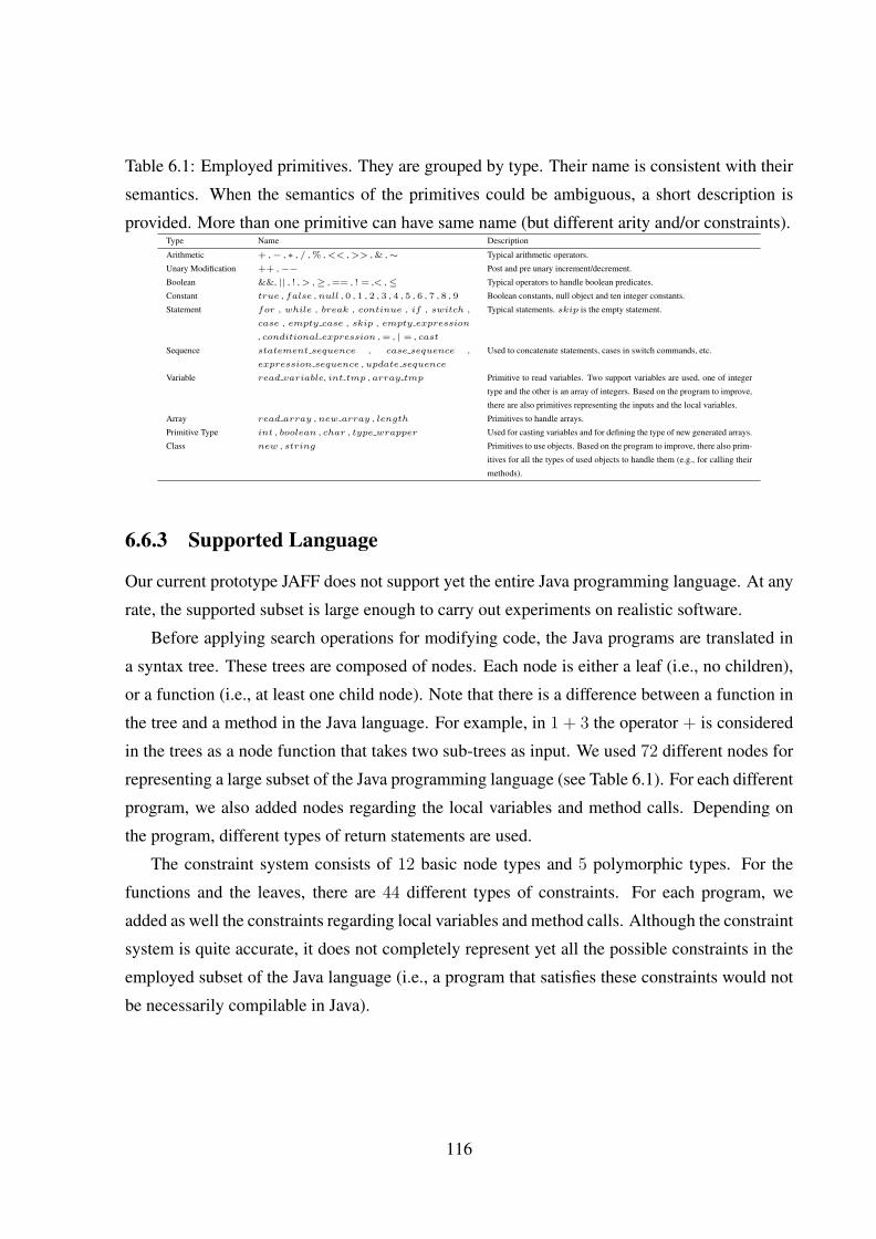
Table 6.1: Employed primitives. They are grouped by type. Their name is consistent with their
semantics. When the semantics of the primitives could be ambiguous, a short description is
provided. More than one primitive can have same name (but different arity and/or constraints).Type Name Description
Arithmetic + ,− , ∗ , / , % ,<< ,>> , & ,∼ Typical arithmetic operators.
Unary Modification ++ ,−− Post and pre unary increment/decrement.
Boolean &&, || , ! ,> ,≥ , == , ! = ,< ,≤ Typical operators to handle boolean predicates.
Constant true , false , null , 0 , 1 , 2 , 3 , 4 , 5 , 6 , 7 , 8 , 9 Boolean constants, null object and ten integer constants.
Statement for , while , break , continue , if , switch ,
case , empty case , skip , empty expression
, conditional expression , = , | = , cast
Typical statements. skip is the empty statement.
Sequence statement sequence , case sequence ,
expression sequence , update sequence
Used to concatenate statements, cases in switch commands, etc.
Variable read variable, int tmp , array tmp Primitive to read variables. Two support variables are used, one of integer
type and the other is an array of integers. Based on the program to improve,
there are also primitives representing the inputs and the local variables.
Array read array , new array , length Primitives to handle arrays.
Primitive Type int , boolean , char , type wrapper Used for casting variables and for defining the type of new generated arrays.
Class new , string Primitives to use objects. Based on the program to improve, there also prim-
itives for all the types of used objects to handle them (e.g., for calling their
methods).
6.6.3 Supported Language
Our current prototype JAFF does not support yet the entire Java programming language. At any
rate, the supported subset is large enough to carry out experiments on realistic software.
Before applying search operations for modifying code, the Java programs are translated in
a syntax tree. These trees are composed of nodes. Each node is either a leaf (i.e., no children),
or a function (i.e., at least one child node). Note that there is a difference between a function in
the tree and a method in the Java language. For example, in 1 + 3 the operator + is considered
in the trees as a node function that takes two sub-trees as input. We used 72 different nodes for
representing a large subset of the Java programming language (see Table 6.1). For each different
program, we also added nodes regarding the local variables and method calls. Depending on
the program, different types of return statements are used.
The constraint system consists of 12 basic node types and 5 polymorphic types. For the
functions and the leaves, there are 44 different types of constraints. For each program, we
added as well the constraints regarding local variables and method calls. Although the constraint
system is quite accurate, it does not completely represent yet all the possible constraints in the
employed subset of the Java language (i.e., a program that satisfies these constraints would not
be necessarily compilable in Java).
116

6.7 Case Study
6.7.1 Faulty Programs
To validate our novel prototype JAFF, we applied it to a case study. Ideally, validation should be
done on real-world faults. They can be obtained from open source software repositories [238],
in which all the versions of the software are stored. Hence, in many cases, it is possible to
see which faults are in a particular version, and then checking how they have been fixed in the
following versions.
Using real-world software was not possible because our current prototype does not support
the entire Java language specification yet. Furthermore, research on software repair is still at an
early stage, and in this chapter we want to give directions on how to apply search algorithms
to tackle it. We are aware of the many difficulties of this task and that more research is still
required.
Nevertheless, faults in software in open repositories show only one side of the problem. In
general, that type of faults are discovered only after the software has been used for a while. In
many cases, these faults are related to special circumstances that were not considered by the
original programmer. But what about the faults that are fixed before submitting a new version
of the software? It is not uncommon that a developer write a code, test it, it does not work, and
then (s)he spends minutes/hours to fix it, and finally (s)he submits the code only when all the
test cases are passed.
This latter type of faults does not usually appear in open source repositories, and it includes
for example simple errors (e.g., a + instead of a −) that make the program fail on each input.
Depending on the complexity of the software, these faults are not necessarily easy to fix.
Given a set of programs written in a subset of Java that our prototype can handle, we had the
problem of how to seed faults in them. Doing that by hand would likely end up in a biased case
study. We chose to seed the programs with a Mutation Testing [199] tool called muJava [243].
We did it because this type of mutants are actually representative of a range of real errors that
developers can occasionally do [244]. Mutation testing has been shown to be very effective to
evaluate the quality of test cases. In evaluating test cases, the mutants are more close to real-
world faults than faults generated by hand [244]. Furthermore, applying more mutations on
the same program gives us a case study with different degrees of difficulty (we can reasonably
assume that programs that are mutated more are likely more difficult to fix).
To make our case study as little biased as possible, we chose a set of search operators that is
not specialised in fixing faults generated by mutation testing tools. In particular, we just chose
117

all the possible mutation operators in ECJ [158] (we described them in Section 4.2.3), and we
gave the same probability to all of them without any particular bias to any of them. Therefore,
our framework can be used to any code level type of faults, although our case study is limited
to mutation testing faults.
It might be argued that limiting the case study to faults generated by mutation testing tools
is too restrictive. However, repairing software in an automatic way is a very complex task, and a
lot of research is still required for having stronger results. Nevertheless, showing its feasibility
on a sub-set of realistic types of faults is important to support the first steps in this research
field. For example, it has been estimated that 10% of all faults can be fixed with only one line
modification [237, 238]).
We analyse the framework on seven different Java programs. Among them, two are classi-
cally used in the literature of software testing of procedural programs: Triangle Classification
[18] and Remainder [60, 245]. TreeMap and Vector are common in literature of testing object-
oriented software [140]. Sorting algorithms as for example Bubble Sort [180] are commonly
used in literature of GP (e.g., [189]). Finally, Phase of Moon is adapted from Apache Ant [246].
Table 6.2 summarises their properties. Apart from TreeMap and Vector, all the other pro-
grams are static functions. Regarding TreeMap, we carried out experiments only on its method
put. For Vector, we consider the methods insertElementAt and removeElementAt.
It can be argued that the size of these functions is small, i.e. the longest has only 41 lines
of code. However, in this first application of search algorithms on the software repairing task
we limit our self to the single method assumption, which in some empirical studies it has been
estimated to be valid for half of real-world faults (see Section 6.3.3).
Note that for TreeMap and Vector there are many private methods that are used inside the
analysed three methods, but they are assumed to be correct during the search. Because a priori
we would not know which of these methods is faulty, we should do a search in each of these
methods in parallel (see Section 6.3.3). If we ignore the case that a modification in a correct
method does fix the fault generated by the faulty method that calls it, we do not need to run
these parallel searches in our experiments. Given t steps needed to fix a fault in one of these
faulty methods, to estimated the required computational effort we can just multiply this t by the
number of involved methods (under the assumption we are not focusing the search in any of
them). Note that parallel searches can be done even on a single CPU machine (the parallelism
would be simply simulated).
For each program, we generated a set of 100 test cases. Each test case consists of one assert
statement, but for TreeMap and Vector there is an assert statement for each insertion operation
118

Table 6.2: For each program in the case study, it is shown its number of lines of code (LOC),
the number of nodes in its syntax tree representation, and finally the type of its inputs.Name LOC GP Nodes Input
Phase of Moon 8 50 int,int
Vector.insertElementAt 9 53 Object,int
Bubble Sort 10 56 int[]
Vector.removeElementAt 16 62 int
Triangle Classification 25 101 int,int,int
TreeMap.put 36 134 Object,Object
Remainder 41 160 int,int
in the test sequence, and a final assertion on the container size (i.e., around four/five assertions
for test case). We call valid all the evolved programs that are able to pass all of their 100 test
cases. For more validation, we also generated for each program a separated and independent
set of 1000 test cases, which are not used during the search. An evolved program that is able
to pass all these 1000 test cases is called robust. Note that a robust program is not necessarily
correct.
All the test cases have been automatically generated based on the fulfilment of the branch
coverage criterion. For simplicity, in our experiments we used test generators specialised for
our case study. To apply our framework to a new testing problem, the user has to provide the
test cases.
For each program, we generated 5 faulty versions. The first is done by a single mutation
with muJava, the second by applying a new mutation on the first faulty version (i.e., 2 mutations
in total), and so on until the 5th that has been generated by applying a new mutation on the 4th
version (i.e., 5 mutations in total). The mutations were chosen at random, although we replaced
the ones that generated equivalent mutants. We used all the method level mutations in muJava
(more details about them can be found in [243]).
Table 6.3 summaries the number of assertions that are passed in each faulty version. Note
that a higher number of mutations does not necessarily correspond to fewer passed test cases
(see for example the Phase of Moon program). This is a clear example of possible local optima.
119

Table 6.3: Number of passed assertions in the faulty versions of the programs.Program V1 V2 V3 V4 V5
Phase of Moon 0 0 0 0 11
Vector.insertElementAt 262 8 8 8 8
Bubble Sort 32 32 34 32 44
Vector.removeElementAt 180 251 233 250 250
Triangle Classification 86 60 46 44 27
TreeMap.put 86 24 24 24 38
Remainder 83 76 63 55 55
6.7.2 Setting of the Framework
For the employed search algorithms, we used the default values in ECJ [158], unless otherwise
specified in the chapter. The maximum tree depth is 25. The maximum number of allowed
fitness evaluations is 50,000. The computation is stopped in the case that a program that passes
all the test cases is found.
For the GP algorithm, population size is 1000 (hence the maximum number of generations
is 50). A tournament selection with size 7 is employed. The elitism rate is set to 1 individual
for generation. The main search operator is mutation, that is done with probability 0.9. We still
use crossover, but with a very low probability of 0.08. A tree is left unmodified with probability
0.01, whereas with probability 0.01 it is replaced with the original faulty program (this is done
for forcing the presence of its genetic material at each generation).
Note that we have not tuned these values. The reason is explained in Section 6.7.4 after the
experiments.
6.7.3 Experiments
We carried out three different sets of experiments:
1. For each faulty program, we tuned the parameter M (max number of mutations) for RS.
Considered values are in range from 1 to 10. Each run has been repeated 100 times with
different random seeds. The total number of runs is hence 5 ∗ 7 ∗ 10 ∗ 100 = 35,000.
2. For each faulty program, we tuned the parameter M (max number of mutations) for HC.
Considered values are in range from 1 to 10. Each run has been repeated 100 times with
different random seeds. The total number of runs is hence 5 ∗ 7 ∗ 10 ∗ 100 = 35,000.
120

3. For each faulty program, we run the GP algorithm. We tested the novel search operator
with values of the node bias ranging from 1 to 10. Each run has been repeated 100 times
with different random seeds. The total number of runs is hence 5 ∗ 7 ∗ 10 ∗ 100 = 35,000.
The total number of runs of the framework used for collecting data is 105,000. This is a large
number of experiments that can take up a long time to run. A larger case study would necessarily
reduce the number of types of experiments and the number of repetitions (with different random
seeds) for each experiment.
For these experiments, the number of robust programs that are obtained are shown in Figure
6.2, Figure 6.3 and Figure 6.4. The best value for the parameter M for RS is 4 (first set of
experiments, Figure 6.2), whereas for HC it is 7 (second set of experiments, Figure 6.3). Tables
from 6.4 to Table 6.10 compare the tuned RS against the tuned HC and a non-tuned GP. Tables
from 6.11 to Table 6.17 compare GP when the novel operator is used with tournament size (i.e.,
node bias) 2.
The event of sampling a valid and/or a robust program can be modelled as a binomial pro-
cess. Therefore, Fisher’s Exact tests can be used to see whether there is any statistical difference
between the success rate of two different algorithms or configurations.
6.7.4 Discussion
The experiments we carried out show that each of the 35 faulty programs can be automatically
corrected with our tool JAFF. Of course, depending on the complexity of the software and the
faults, these results are achieved with different computational effort.
Not surprisingly, when only few faults are considered (i.e., V 1 and V 2), the performance
of RS and GP are very similar. But for more complex types of faults (i.e., V 4 and V 5) GP
clearly stands out from the other considered algorithms (Fisher’s exact tests confirm it in many
cases). This is one reason why we did not need to tune the parameters of GP. Already with some
arbitrarily setting it performs better then tuned RS and HC.
What came as a surprise is the performance of HC, which is very poor. One explanation
would be that there can be many small modifications that can improve the fitness, but that then
drive the current solution away from the global optima. Once HC is driven to such a suboptimal
region, the use of large jumps (i.e., the number of mutations applied to generate the neighbour
solutions) seems to be not enough to escape from them. However, more sophisticated variants
of HC could be designed.
Figure 6.4 clearly shows that the novel search operator is useful in many cases, but for
121

Table 6.4: Comparison for Phase of MoonVersion Algorithm Valid Robust Steps Size
min mean median max var min mean median max var
V1 RS 100 95 60 2137.13 1230.0 12482 5740488.0 46 50.63 50.0 57 2.336465
HC 0 0 50000 50000.0 50000.0 50000 0.0 41 52.28 53.0 61 30.56727
GP 92 71 1981 7874.73 1993.0 50000 1.80482595E8 40 51.33 50.0 114 49.07182
V2 RS 100 94 16 1203.29 844.0 6708 1657107.0 47 50.97 51.0 56 1.605152
HC 1 0 1364 49515.62 50000.0 50000 2.365655E7 41 53.19 53.0 61 34.23626
GP 98 80 1973 4078.29 1993.0 50000 5.5358582E7 46 51.92 51.0 79 12.33697
V3 RS 83 10 406 22460.47 18012.0 50000 3.0671632E8 45 50.4 51.0 66 7.878788
HC 0 0 50000 50000.0 50000.0 50000 0.0 41 52.72 53.0 61 33.05212
GP 98 8 2962 6551.3 4959.0 50000 4.7339725E7 41 50.71 51.0 62 11.94535
V4 RS 19 2 2544 45313.18 50000.0 50000 1.28933411E8 45 52.15 52.0 61 5.926768
HC 2 0 531 49046.58 50000.0 50000 4.5238729E7 42 53.95 55.0 62 34.59343
GP 88 7 3959 11863.57 5942.0 50000 2.18956904E8 41 52.6 52.0 107 48.78788
V5 RS 0 0 50000 50000.0 50000.0 50000 0.0 47 51.78 51.0 57 3.203636
HC 0 0 50000 50000.0 50000.0 50000 0.0 44 56.15 57.0 63 34.33081
GP 8 0 4972 48350.73 50000.0 50000 6.7942853E7 44 60.72 59.0 176 257.3349
higher values of the node bias n the performance starts to decrease (this is in accordance with
Equation 6.4). When n = 2, a closer look at Tables from 6.11 to 6.17 shows that for simple
types of faults (i.e., V 1 and V 2), there is not much difference in the performance (whether it is
an improvement or a decrease of performance). For more complex faults (i.e., V 4 and V 5) it
seems that the novel operator gives significantly better results (Fisher’s exact tests confirm it for
Remainder and TreeMap).
It is interesting to see whether in this particular type of application of GP we would get
bloat or no. Unfortunately, bloat does occur. For example, the largest program we obtained is
for Remainder (see Table 6.12). A final size of 430 nodes was obtained from a starting program
with size 160.
Most of the time, a valid solution was also robust. That is a very important result, because it
means that in general the patches generated by the JAFF are fixing the actual faults (at least in
our case study). Given a set of test cases, there is an infinite number of semantically different
programs that fit them. However, their distribution in the search space is in general not known,
and they might be very far from each other. Fortunately, the experiments show that “near” a
correct solution there are only few programs that are valid but not robust.
6.8 Limitations
The task of repairing software is very challenging. Regardless of the employed technique, there
are serious problems that limit the automation of this task:
• Testing cannot prove that a program is faultless [18]. Therefore, the task of fixing faults
122

2 4 6 8 10
020
4060
8010
0
Remainder
Mutations
Rob
ust %
2 4 6 8 10
020
4060
8010
0
Bubble_Sort
Mutations
Rob
ust %
2 4 6 8 10
020
4060
8010
0
TreeMap.put
Mutations
Rob
ust %
2 4 6 8 10
020
4060
8010
0
Triangle_Classification
Mutations
Rob
ust %
2 4 6 8 10
020
4060
8010
0
Vector.insert
Mutations
Rob
ust %
2 4 6 8 10
020
4060
8010
0
Vector.remove
Mutations
Rob
ust %
2 4 6 8 10
020
4060
8010
0
Phase_of_Moon
Mutations
Rob
ust %
Figure 6.2: Results of tuning the value of maximum number of mutations for RS. Proportion of
obtained robust programs are shown. Data were collected from 100 runs of the framework with
different random seeds. There are 7 plots, one for each program in the case study. Each plot
contains the results for each of the 5 faulty versions of that program.123

2 4 6 8 10
020
4060
8010
0
Remainder
Neighbourhood Size
Rob
ust %
2 4 6 8 10
020
4060
8010
0
Bubble_Sort
Neighbourhood Size
Rob
ust %
2 4 6 8 10
020
4060
8010
0
TreeMap.put
Neighbourhood Size
Rob
ust %
2 4 6 8 10
020
4060
8010
0
Triangle_Classification
Neighbourhood Size
Rob
ust %
2 4 6 8 10
020
4060
8010
0
Vector.insert
Neighbourhood Size
Rob
ust %
2 4 6 8 10
020
4060
8010
0
Vector.remove
Neighbourhood Size
Rob
ust %
2 4 6 8 10
020
4060
8010
0
Phase_of_Moon
Neighbourhood Size
Rob
ust %
Figure 6.3: Results of tuning the value of maximum number of mutations (i.e., the neighbour-
hood size) for HC. Proportion of obtained robust programs are shown. Data were collected from
100 runs of the framework with different random seeds. There are 7 plots, one for each program
in the case study. Each plot contains the results for each of the 5 faulty versions of that program.124

2 4 6 8 10
020
4060
8010
0
Remainder
Node Bias
Rob
ust %
2 4 6 8 10
020
4060
8010
0
Bubble_Sort
Node Bias
Rob
ust %
2 4 6 8 10
020
4060
8010
0
TreeMap.put
Node Bias
Rob
ust %
2 4 6 8 10
020
4060
8010
0
Triangle_Classification
Node Bias
Rob
ust %
2 4 6 8 10
020
4060
8010
0
Vector.insert
Node Bias
Rob
ust %
2 4 6 8 10
020
4060
8010
0
Vector.remove
Node Bias
Rob
ust %
2 4 6 8 10
020
4060
8010
0
Phase_of_Moon
Node Bias
Rob
ust %
Figure 6.4: Results of GP using the novel search operator with different values n for the node
bias. Proportion of obtained robust programs are shown. Data were collected from 100 runs of
the framework with different random seeds. There are 7 plots, one for each program in the case
study. Each plot contains the results for each of the 5 faulty versions of that program.125

Table 6.5: Comparison for RemainderVersion Algorithm Valid Robust Steps Size
min mean median max var min mean median max var
V1 RS 100 99 12 4240.81 2655.0 21122 1.9694475E7 156 160.18 160.0 165 1.724848
HC 19 18 4 42022.78 50000.0 50000 2.96175183E8 152 163.07 161.0 170 24.5102
GP 100 99 1977 3742.28 2980.0 11886 5275823.0 151 163.69 160.0 189 65.16556
V2 RS 0 0 50000 50000.0 50000.0 50000 0.0 150 158.91 160.0 168 12.16354
HC 17 17 661 43124.64 50000.0 50000 2.56260183E8 151 163.72 164.5 170 37.39556
GP 88 87 3971 16349.27 10886.0 50000 2.03742456E8 149 195.33 166.5 311 2888.425
V3 RS 0 0 50000 50000.0 50000.0 50000 0.0 149 158.29 158.5 166 11.15747
HC 9 9 1382 46693.64 50000.0 50000 1.36677492E8 150 160.9479 160.0 171 30.78673
GP 91 90 6942 19308.98 14863.0 50000 1.44971481E8 151 183.11 163.5 312 2108.867
V4 RS 0 0 50000 50000.0 50000.0 50000 0.0 149 159.12 160.0 167 9.379394
HC 0 0 50000 50000.0 50000.0 50000 0.0 150 160.63 160.0 170 29.06374
GP 42 42 11907 39718.67 50000.0 50000 2.03653224E8 150 172.79 161.0 430 1796.875
V5 RS 0 0 50000 50000.0 50000.0 50000 0.0 147 160.1 161.0 169 10.87879
HC 1 0 26127 49763.25 50000.0 50000 5700156.0 152 162.78 163.0 171 23.48646
GP 24 24 12862 43855.15 50000.0 50000 1.52540938E8 145 164.12 161.0 306 467.9248
Table 6.6: Comparison for Bubble SortVersion Algorithm Valid Robust Steps Size
min mean median max var min mean median max var
V1 RS 100 100 11 765.78 561.5 5277 577521.9 56 56.3 56.0 61 0.7171717
HC 15 15 4 43418.5 50000.0 50000 2.56884057E8 48 57.84 56.0 66 15.73172
GP 100 100 1983 2120.11 1991.0 10888 842416.3 56 56.14 56.0 63 0.7276768
V2 RS 95 95 8 12522.17 7891.0 50000 1.60618102E8 46 57.44 58.0 62 3.25899
HC 7 7 12 46904.21 50000.0 50000 1.41018839E8 49 59.21 58.0 68 23.29889
GP 100 100 2966 4314.74 3968.0 12882 3325363.0 56 58.2 58.0 72 6.141414
V3 RS 10 10 14682 47896.13 50000.0 50000 4.9980018E7 54 58.2 58.0 66 3.313131
HC 4 3 209 48120.73 50000.0 50000 8.606186E7 49 62.74 63.0 69 26.82061
GP 61 61 9901 34550.55 32167.0 50000 2.07041549E8 51 67.26 65.0 159 189.7095
V4 RS 0 0 50000 50000.0 50000.0 50000 0.0 50 58.33 59.0 67 5.132424
HC 1 1 2754 49529.52 50000.0 50000 2.2323735E7 50 61.81 60.0 69 27.26657
GP 40 40 11873 39988.8 50000.0 50000 1.88839409E8 51 65.73 66.0 145 92.54253
V5 RS 0 0 50000 50000.0 50000.0 50000 0.0 51 59.29 61.0 65 12.28879
HC 0 0 50000 50000.0 50000.0 50000 0.0 61 61.0 61.0 61 0.0
GP 4 4 13819 49419.68 50000.0 50000 2.7698504E7 51 64.67 65.0 96 33.94051
Table 6.7: Comparison for TreeMap.putVersion Algorithm Valid Robust Steps Size
min mean median max var min mean median max var
V1 RS 100 100 7 290.47 215.5 1455 83048.72 124 133.55 134.0 138 6.04798
HC 33 31 9 33974.3 50000.0 50000 5.34342344E8 109 128.81 129.0 142 38.09485
GP 100 100 1977 2000.55 1991.0 2986 9930.129 134 134.1 134.0 135 0.0909091
V2 RS 98 93 70 12949.75 7569.0 50000 1.6773158E8 121 134.15 134.0 138 5.421717
HC 10 6 130 46557.72 50000.0 50000 1.32885341E8 116 130.6 130.0 141 24.10101
GP 98 93 1991 7233.5 6924.0 50000 4.5553323E7 89 129.78 133.0 223 270.1733
V3 RS 98 88 87 13037.58 9616.0 50000 1.29265796E8 125 134.98 135.0 141 8.807677
HC 11 9 76 46057.19 50000.0 50000 1.49424541E8 125 131.96 131.0 145 21.45293
GP 98 96 1993 7074.34 5952.0 50000 4.8643077E7 108 131.67 133.5 223 135.8799
V4 RS 100 100 69 4047.41 2787.0 22842 1.5242408E7 119 130.78 129.0 142 28.51677
HC 26 26 33 40880.0 50000.0 50000 3.32099098E8 126 133.6471 135.5 140 15.20499
GP 100 100 2962 3622.98 3959.0 4974 482048.5 125 132.73 131.0 171 47.61323
V5 RS 23 22 1152 43768.76 50000.0 50000 1.76661972E8 126 134.3553 136.0 145 31.91211
HC 16 16 724 44681.98 50000.0 50000 1.88406817E8 126 133.2143 134.5 142 18.95296
GP 77 72 4950 23305.71 13344.0 50000 3.24309559E8 107 135.2 134.0 203 184.0404
126

Table 6.8: Comparison for Triangle ClassificationVersion Algorithm Valid Robust Steps Size
min mean median max var min mean median max var
V1 RS 100 100 9 726.9 451.5 3184 465492.1 79 98.31 101.0 106 24.84232
HC 78 76 6 12933.87 148.0 50000 4.40213802E8 82 97.42 99.0 110 30.00364
GP 100 100 1977 2296.69 1993.0 3959 230680.4 89 100.17 101.0 106 7.879899
V2 RS 90 81 1049 11327.27 5309.0 50000 2.19276055E8 93 100.9091 102.0 106 12.09091
HC 52 47 7 33179.78 49224.0 50000 4.4634373E8 92 100.6957 102.0 111 20.31225
GP 100 99 2964 4048.86 3971.0 7927 826978.2 89 103.23 101.0 174 215.8961
V3 RS 45 45 1049 38412.36 50000.0 50000 2.69787927E8 90 97.81818 99.0 103 18.76364
HC 28 21 38 36302.93 50000.0 50000 5.08828403E8 86 97.0 97.0 105 22.30769
GP 100 99 3957 5067.24 4962.0 6946 570266.1 82 100.54 97.0 193 289.2812
V4 RS 26 24 318 43461.23 50000.0 50000 1.86471282E8 87 98.45205 101.0 107 21.5567
HC 13 13 88 44285.41 50000.0 50000 2.16766584E8 92 99.93103 101.0 109 18.99507
GP 100 92 2986 4986.76 4956.0 6956 602590.7 81 102.2 98.0 204 407.596
V5 RS 0 0 50000 50000.0 50000.0 50000 0.0 97 100.4776 101.0 104 4.919946
HC 7 7 10290 46947.23 50000.0 50000 1.21310996E8 94 100.2308 99.0 108 21.35897
GP 100 94 4944 7142.54 6935.5 21755 3617325.0 80 106.9 101.0 203 641.9091
Table 6.9: Comparison for Vector.insertElementAtVersion Algorithm Valid Robust Steps Size
min mean median max var min mean median max var
V1 RS 100 60 9 415.63 283.5 1834 145470.7 44 53.52 53.0 59 3.969293
HC 86 80 5 13274.09 1794.5 50000 3.48679583E8 44 52.04 51.0 64 14.38222
GP 100 49 1977 2001.29 1991.0 2992 10032.29 51 53.72 53.0 57 1.153131
V2 RS 38 27 1409 39237.6 50000.0 50000 2.66236149E8 32 52.07 53.0 60 12.38899
HC 47 44 97 34150.1 50000.0 50000 3.92340786E8 43 51.81 51.0 64 27.26657
GP 100 80 2973 7576.95 6935.0 19784 1.2007509E7 36 53.19 53.0 86 34.80192
V3 RS 0 0 50000 50000.0 50000.0 50000 0.0 33 47.61 49.0 61 48.1797
HC 22 21 104 41622.72 50000.0 50000 3.00193727E8 43 51.05 50.5 63 26.55303
GP 95 91 7906 16463.11 13885.0 50000 8.5745263E7 31 57.76 55.0 119 235.0125
V4 RS 0 0 50000 50000.0 50000.0 50000 0.0 27 44.06 44.0 60 77.93576
HC 12 12 23892 47807.71 50000.0 50000 3.9387227E7 34 51.51613 54.0 57 26.65806
GP 85 81 8817 20418.05 15520.0 50000 1.75634471E8 40 54.53 50.5 104 140.5546
V5 RS 0 0 50000 50000.0 50000.0 50000 0.0 32 52.22 53.5 63 30.13293
HC 0 0 50000 50000.0 50000.0 50000 0.0 50 54.83 54.0 62 2.506162
GP 60 57 11893 35015.14 30688.5 50000 2.01166805E8 36 55.37 53.5 114 138.4779
Table 6.10: Comparison for Vector.removeElementAtVersion Algorithm Valid Robust Steps Size
min mean median max var min mean median max var
V1 RS 100 100 21 1852.94 1446.0 11719 3236402.0 49 61.62 62.0 67 6.94505
HC 9 9 538 46370.06 50000.0 50000 1.54333325E8 52 60.89 61.0 72 20.09889
GP 94 93 1981 8528.23 2978.0 50000 1.51724089E8 45 61.87 62.0 70 11.42737
V2 RS 97 95 186 14866.05 11146.0 50000 1.54956132E8 47 60.68 62.0 66 8.866263
HC 7 6 1174 47277.12 50000.0 50000 1.15798437E8 47 61.28 62.0 71 18.8097
GP 95 67 2980 11907.98 8927.0 50000 9.5283106E7 42 60.27 60.5 89 48.50212
V3 RS 21 21 7518 44952.85 50000.0 50000 1.33729877E8 46 59.68 60.0 67 16.03798
HC 4 4 2125 48873.3 50000.0 50000 4.5676465E7 50 60.99 61.0 71 17.94939
GP 96 93 3963 11335.36 8896.0 50000 8.3188229E7 35 59.59 59.0 108 68.48677
V4 RS 5 5 3153 48750.37 50000.0 50000 4.113287E7 51 59.35 60.0 68 11.05808
HC 3 3 3670 48854.61 50000.0 50000 4.6501996E7 52 62.56 62.0 71 5.945859
GP 94 93 3967 16241.65 13856.0 50000 1.10595009E8 37 57.61 57.0 77 39.95747
V5 RS 0 0 50000 50000.0 50000.0 50000 0.0 40 58.56 59.5 69 22.18828
HC 0 0 50000 50000.0 50000.0 50000 0.0 62 62.0 62.0 62 0.0
GP 41 41 8926 38049.46 50000.0 50000 2.5916941E8 43 60.77 61.0 72 37.65364
127

Table 6.11: Node bias for Phase of MoonVersion Node Bias Valid Robust Steps Size
min mean median max var min mean median max var
V1 1 92 71 1981 7874.73 1993.0 50000 1.80482595E8 40 51.33 50.0 114 49.07182
2 93 61 1981 7608.9 1995.0 50000 1.59994246E8 45 52.81 50.0 111 94.33727
V2 1 98 80 1973 4078.29 1993.0 50000 5.5358582E7 46 51.92 51.0 79 12.33697
2 97 86 1981 4918.8 1993.0 50000 9.7081664E7 49 52.55 51.0 104 46.08838
V3 1 98 8 2962 6551.3 4959.0 50000 4.7339725E7 41 50.71 51.0 62 11.94535
2 97 14 2970 6718.12 4956.0 50000 6.7456329E7 45 52.24 51.0 111 85.7398
V4 1 88 7 3959 11863.57 5942.0 50000 2.18956904E8 41 52.6 52.0 107 48.78788
2 96 9 2977 8152.61 5947.0 50000 8.6429858E7 43 51.74 52.0 82 24.03273
V5 1 8 0 4972 48350.73 50000.0 50000 6.7942853E7 44 60.72 59.0 176 257.3349
2 14 1 6918 45919.05 50000.0 50000 1.43511683E8 43 57.78 58.0 94 61.95111
Table 6.12: Node bias for RemainderVersion Node Bias Valid Robust Steps Size
min mean median max var min mean median max var
V1 1 100 99 1977 3742.28 2980.0 11886 5275823.0 151 163.69 160.0 189 65.16556
2 100 100 1981 3386.31 1997.0 8926 4389840.0 152 162.36 160.0 183 39.9499
V2 1 88 87 3971 16349.27 10886.0 50000 2.03742456E8 149 195.33 166.5 311 2888.425
2 94 93 2964 11415.94 8922.0 50000 1.08120192E8 150 189.09 166.0 340 2414.083
V3 1 91 90 6942 19308.98 14863.0 50000 1.44971481E8 151 183.11 163.5 312 2108.867
2 92 92 4968 15168.0 11876.0 50000 1.33802121E8 149 191.82 162.5 414 3574.129
V4 1 42 42 11907 39718.67 50000.0 50000 2.03653224E8 150 172.79 161.0 430 1796.875
2 56 55 5949 33459.62 27194.5 50000 2.60867209E8 147 172.44 161.0 383 1573.825
V5 1 24 24 12862 43855.15 50000.0 50000 1.52540938E8 145 164.12 161.0 306 467.9248
2 55 52 12882 36685.23 41038.5 50000 1.98223693E8 146 177.08 163.0 395 1787.953
Table 6.13: Node bias for Bubble SortVersion Node Bias Valid Robust Steps Size
min mean median max var min mean median max var
V1 1 100 100 1983 2120.11 1991.0 10888 842416.3 56 56.14 56.0 63 0.7276768
2 100 100 1977 3068.04 1993.0 19797 8760304.0 56 56.47 56.0 64 2.332424
V2 1 100 100 2966 4314.74 3968.0 12882 3325363.0 56 58.2 58.0 72 6.141414
2 99 99 2971 5511.96 3978.0 50000 2.9593816E7 56 58.92 58.0 85 24.51879
V3 1 61 61 9901 34550.55 32167.0 50000 2.07041549E8 51 67.26 65.0 159 189.7095
2 58 57 9881 37723.4 40544.0 50000 1.70364011E8 54 69.21 67.0 133 182.6726
V4 1 40 40 11873 39988.8 50000.0 50000 1.88839409E8 51 65.73 66.0 145 92.54253
2 32 32 12868 43375.54 50000.0 50000 1.40733504E8 54 67.9 66.0 128 143.8687
V5 1 4 4 13819 49419.68 50000.0 50000 2.7698504E7 51 64.67 65.0 96 33.94051
2 11 11 14850 48615.09 50000.0 50000 3.8011468E7 53 66.61 67.0 117 50.86657
Table 6.14: Node bias for TreeMap.putVersion Node Bias Valid Robust Steps Size
min mean median max var min mean median max var
V1 1 100 100 1977 2000.55 1991.0 2986 9930.129 134 134.1 134.0 135 0.0909091
2 100 100 1975 1990.78 1991.0 2001 26.57737 134 134.11 134.0 135 0.09888889
V2 1 98 93 1991 7233.5 6924.0 50000 4.5553323E7 89 129.78 133.0 223 270.1733
2 100 99 1991 4820.31 3974.5 9881 3988607.0 103 130.63 134.0 182 79.42737
V3 1 98 96 1993 7074.34 5952.0 50000 4.8643077E7 108 131.67 133.5 223 135.8799
2 100 96 1993 4533.07 3963.0 7937 3361239.0 116 132.93 135.0 157 40.69202
V4 1 100 100 2962 3622.98 3959.0 4974 482048.5 125 132.73 131.0 171 47.61323
2 100 100 1987 3157.16 2982.0 3981 185676.7 126 132.78 130.5 231 121.6279
V5 1 77 72 4950 23305.71 13344.0 50000 3.24309559E8 107 135.2 134.0 203 184.0404
2 91 90 1983 16015.66 8919.0 50000 2.29592935E8 116 136.72 136.0 201 114.8299
128

Table 6.15: Node bias for Triangle ClassificationVersion Node Bias Valid Robust Steps Size
min mean median max var min mean median max var
V1 1 100 100 1977 2296.69 1993.0 3959 230680.4 89 100.17 101.0 106 7.879899
2 100 100 1980 2077.368 1991.0 2994 80329.13 91 100.6842 101.0 105 3.398496
V2 1 100 99 2964 4048.86 3971.0 7927 826978.2 89 103.23 101.0 174 215.8961
2 100 100 2964 3731.582 3963.0 4972 508542.2 88 105.0759 101.0 192 380.9172
V3 1 100 99 3957 5067.24 4962.0 6946 570266.1 82 100.54 97.0 193 289.2812
2 100 100 3949 4581.29 4940.0 5955 448987.5 84 100.68 97.0 201 389.9976
V4 1 100 92 2986 4986.76 4956.0 6956 602590.7 81 102.2 98.0 204 407.596
2 100 90 3943 4581.65 4948.0 5957 373174.3 88 101.07 97.5 202 354.0254
V5 1 100 94 4944 7142.54 6935.5 21755 3617325.0 80 106.9 101.0 203 641.9091
2 100 90 3954 6273.2 5954.0 9899 1144242.0 81 106.96 97.5 202 787.7964
Table 6.16: Node bias for Vector.insertElementAtVersion Node Bias Valid Robust Steps Size
min mean median max var min mean median max var
V1 1 100 49 1977 2001.29 1991.0 2992 10032.29 51 53.72 53.0 57 1.153131
2 100 63 1977 2020.66 1991.0 2986 28935.6 49 53.59 53.0 57 1.436263
V2 1 100 80 2973 7576.95 6935.0 19784 1.2007509E7 36 53.19 53.0 86 34.80192
2 100 84 2974 7332.65 5957.5 20767 1.4407158E7 38 53.46 53.0 112 74.67515
V3 1 95 91 7906 16463.11 13885.0 50000 8.5745263E7 31 57.76 55.0 119 235.0125
2 96 89 5947 15653.79 14822.0 50000 6.6893394E7 25 56.76 53.0 109 213.1539
V4 1 85 81 8817 20418.05 15520.0 50000 1.75634471E8 40 54.53 50.5 104 140.5546
2 86 79 6923 21071.49 15826.5 50000 1.81154133E8 25 54.37 53.0 102 141.3062
V5 1 60 57 11893 35015.14 30688.5 50000 2.01166805E8 36 55.37 53.5 114 138.4779
2 68 67 11889 33733.53 29624.0 50000 1.89767898E8 28 56.45 55.0 181 254.0682
Table 6.17: Node bias for Vector.removeElementAtVersion Node Bias Valid Robust Steps Size
min mean median max var min mean median max var
V1 1 94 93 1981 8528.23 2978.0 50000 1.51724089E8 45 61.87 62.0 70 11.42737
2 89 88 1981 10108.82 1993.0 50000 2.71177338E8 46 62.15 62.0 74 11.42172
V2 1 95 67 2980 11907.98 8927.0 50000 9.5283106E7 42 60.27 60.5 89 48.50212
2 94 65 3965 13215.6 9901.0 50000 1.15128681E8 47 61.06 61.0 124 82.11758
V3 1 96 93 3963 11335.36 8896.0 50000 8.3188229E7 35 59.59 59.0 108 68.48677
2 96 92 3971 11534.18 8422.5 50000 8.8814779E7 46 58.15 57.0 80 42.2904
V4 1 94 93 3967 16241.65 13856.0 50000 1.10595009E8 37 57.61 57.0 77 39.95747
2 97 96 4966 13323.57 10903.5 50000 6.5809471E7 38 56.57 57.0 94 51.29808
V5 1 41 41 8926 38049.46 50000.0 50000 2.5916941E8 43 60.77 61.0 72 37.65364
2 32 32 9901 40655.23 50000.0 50000 2.17841782E8 48 60.82 61.0 73 34.69455
129

cannot be completely automated, regardless of the technique that we use. Although the
modified program that we obtain might pass all the given test cases, the introduced mod-
ifications might fix the program only for these inputs and they might introduce unwanted
side effects. Figure 6.5 shows a simple example of a program that is able to pass all of
its test cases although it is not correct. Hence, it is necessary that the developers check
the modifications (i.e., the patch) done by the repairing algorithm, and this task cannot
be automated (unless a formal way to prove its correctness is given, and that can be done
only in trivial cases).
Even if a patch does not actually fix the fault, it gives useful information to the developers.
In fact, that information can be used as a way to locate the area of the code that is related
to the manifestation of the fault. If the developer thinks that the proposed patch is not
correct, he can provide more test cases for which the program fails and then rerun the
framework again.
• A patch can reduce the efficiency of the code, e.g. it can make the software slower.
However, the optimisation of non-functional criteria can be included in the search (see
Chapter 7).
• When we evaluate a modified program to check whether it is correct, the modifications
we apply can make the program to enter in an infinite loop. The Halting Problem [180]
is undecidable. We have to put time limits for the evaluation of modified programs on the
test cases. The threshold could be estimated with heuristics based on the run of the faulty
program on the test cases. A wrong estimation could severally harm the search.
• The modifications done to a program can be difficult to read. This is a common problem
for example in GP. The readability of the code can be included in the objective to optimise.
A simple heuristic would be to prefer, between two correct modified programs, the one
that is more similar to the faulty input program.
• To check if a modified program is correct, we validate it against a set of test cases. Even
with an efficient repairing algorithm, still many programs would likely be required to be
evaluated during the search. If the execution of the test cases is computationally very
expensive (this depends on the type of software), the computational cost of the repairing
task would proportionally increase and likely it would become unpractical.
• Unless a formal specification is provided, the efficacy of repairing algorithms depends on
the quality of the provided test cases. Quality of a set of test cases can be for example
130

<(5,-2,3), 0> // 0 represents ’not triangle’
<(4,3,6) , 1> // 1 represents ’scalene’
<(9,9,16), 2> // 2 represents ’isosceles’
<(3,3,3) , 3> // 3 represents ’equilateral’
function classifyTriangle(a, b, c)
return a + b - c;
Figure 6.5: An example of a test cases for the Triangle Classification problem [18] and an
incorrect simple program that actually is able to pass all of these test cases.
measured with coverage criteria [18]. More and better test cases would result in improved
performance of the repairing algorithm. Even with an ideal repairing algorithm, we cannot
expect good results if the test cases are too few and of low quality. This is similar to the
problem of the choice of test cases for fault localization techniques [247].
6.9 Conclusion
In this chapter we have presented JAFF, the first prototype for the novel approach of repairing
software in an automatic way with search algorithms. In contrast to the literature on the subject,
in our system there is no particular restriction on the type of source code fault that can be fixed.
However, exploiting the properties of real-world faults is helpful to reduce the search space.
Automatically repairing software is the natural next step after the automation of software
testing and fault localization. It is a very complex task, and this chapter gives the contribution
of showing a feasible way to address this problem with evolutionary algorithms. Moreover, we
analysed in detail the properties of this task, with the aim of finding its critical parts that need
to be studied further for improving the performance.
We also presented a novel search operator. We theoretically studied the conditions for which
it gives better results. This search operator improved the performance of our framework in our
case study. This search operator could be extended to other applications where programs with
branches (in the control flow) are tried to be evolved.
Automatic software repair is a difficult task that this chapter addresses with search algo-
rithms. There is still much more research that is required to do before software repair tools can
be used in real-world scenarios:
131

• First step will be to extend JAFF to handle a larger subset of the Java programming lan-
guage. This would allow us to use our prototype to more different types of case studies.
We do not expect that all types of fault can be fixed in an automatic way. An extension of
our framework will help us to better analyse which are the limits of automatic software
repair.
• The search operators play a major role in the success of our technique. This operators
should be optimised to handle faults that are common in real-world software. A deep
analysis of which types of faults actually appear in real-world software is necessary to
design proper search operators. One way to obtain this type of knowledge could be to use
data mining techniques to software repositories (e.g., [214]).
• If a formal specification (e.g., written in either Z [169] or JML [170]) of the software is
provided, we can automatically test all the new changes that we are introducing in the
faulty program (see Chapter 4). We are planning to extend our prototype JAFF to handle
JML.
Given a large set of test cases, co-evolution could be used to choose at each generation a
subset to employ. This could be useful when there are so many test cases that it would
be not efficient to run them all at each fitness evaluation. However, having so many test
cases does not happen often.
• The fitness function of the programs is based on how well they pass their test cases. In our
framework, we support test cases written as unit tests in JUnit [239]. The classes contain-
ing the unit tests need to be automatically instrumented for handling exceptions and for
reporting to the framework whether the test cases are passed or not. The assert statements
can be easily subclassed for giving more gradient to the search (i.e., they should give a
degree of how much an assertion is failed). This is conceptually the same idea of branch
distance in search based software testing (see Section 2.2). Therefore, the same type of
testability transformations [43] can be used to the instrumented unit test classes. We will
investigate the improvement of the results that this technique could bring.
• Hybrid systems that include model checking based tools (see Section 6.2.2) with search
algorithms should be investigated as well.
132

Chapter 7
Automatic Improvement of ExecutionTime
7.1 Motivation
Software1 developers must not only implement code that adheres to the customer’s functional
requirements, but they should also pay attention to performance details. There are many con-
texts in which the execution time is important, for example to aid performance in high-load
server applications, or to maximise time spent in a power-saving mode in software for low-
resource systems. Typical programmer mistakes may include the use of an inefficient algorithm
or data structure, such as employing an Θ(n2) sorting algorithm.
Even if the correct data structures and algorithms are employed, their actual implementations
might still be improved. In general, compilers cannot restructure a program’s implementation
without restriction, even if employing semantics-preserving transformations. The alternative of
relying on manual optimisation is not always possible: the performance implications of design
decisions may be dependent on low-level details hidden from the programmer, or be subject to
subtle interactions with other properties of the software.
To complicate the problem, external factors contribute to the execution time of software,
such as operating system and memory caches events. Taking into account these factors is diffi-
1Part of the work presented in this chapter was carried out in collaboration with Mr. David White, a PhD
student at the University of York and colleague on the SEBASE project. Most of the design work was done
together, and practical work was divided evenly. The author’s contributions focused most on the co-evolutionary
and testing parts of the framework, whereas Mr. White contributed more in the area of multi-objective optimisation
and measurement of non-functional properties.
133

cult, and so compilers usually focus on optimising localised areas of code, rather than restruc-
turing entire functions.
More sophisticated optimisations can be applied if we take into account the probability
distribution of the usage of the software. For example, if a function takes an integer input
and if we know that this input will usually be positive, this information could be exploited by
optimising the software for positive input values.
In this chapter we instantiate our novel framework (Chapter 4) to address the problem of
improving non-functional criteria. In particular, we focus on the improvement of execution
time. Other non-functional criteria could be considered as well, but they are not studied in this
thesis.
Given the code of a function as input to the framework, the optimisations are performed
at the program level and consider the probability distribution of inputs to the program. To our
best knowledge, we do not know of any other system that is able to automatically perform such
optimisations.
Our approach uses multi-objective optimisation (MOO) [142] and Genetic Programming
(GP) (see Section 2.4). In order to preserve semantic integrity whilst improving efficiency, we
apply two sets of test cases. The first is co-evolved with the program population to test the
semantics of the programs. The second is drawn from a distribution modelling expected input,
and is used to assess the non-functional properties of the code. The original function is used as
an oracle to obtain the expected results of these test cases.
Evolving correct software from scratch is a difficult task (see Chapter 5), so we exploit the
code of the input function by seeding the first generation of GP. The first generation will not be a
random sample of the search space as is usually standard in GP applications, but it will contain
genetic material taken from the original input function. Note that this approach is similar to
what we do in our approach for automatic fault correction (see Chapter 6), in which all the
individuals of the first generation were equal to the original incorrect software, and the goal is
to evolve a faultless version.
We present a preliminary implementation of the novel framework, and we validate it on a
case study. We then apply systematic experimentation to determine the most important factors
contributing to the success of the framework. Although our prototype is still in an early stage
of development, this chapter gives the important contribution of presenting a general method to
automatically optimise code using evolutionary techniques. We are also able to provide some
guidance to other practitioners in applying such an approach, based on our analysis of empirical
results.
134
The chapter is organised as follows. Section 7.3 describes in detail all the components of
the framework, whereas Section 7.4 presents our case study. Section 7.5 describes our results
and Section 7.6 describes the current limitations of our novel approach. Finally, Section 7.7
concludes the chapter.
7.2 Related Work
Whilst we are not aware of any work that has proposed a general approach to solving the prob-
lem we outline in this chapter, there are examples of related work in the literature that apply
evolutionary methods within the context of efficiency.
7.2.1 Improving Compiler Performance
Compilers employ a range of techniques to optimise non-functional properties of code [248],
albeit mostly through localised transformations. Most previous work has therefore focused
upon the use of evolutionary techniques at the compiler interface, to find the most effective
combination of such optimisations. For example, evolutionary algorithms have been used to
optimise solution methods for NP problems. Stephenson et al. used GP for solving hyperblock
formation, register allocation and data prefetching [249]. Leventhal et al. used evolutionary
algorithms for offset assignment in digital signal processors [250]. Kri and Feeley used GAs
for register allocation and instruction scheduling problems [251].
Compilers use sequences of code optimisation transformations, and these transformations
are highly correlated to each other. In particular, the order in which they are applied can have a
dramatic impact on the final outcome. The combination and order of selected transformations
can be optimised using evolutionary algorithms: for example, the use of GAs to search for
sequences that reduce code size has been studied by Cooper et al. [57]. Similar work with GAs
has been done by Kulkarni et al. [252], and Fursin et al. used machine learning techniques to
decide which sequence of code optimisation transformations to employ when compiling new
programs [253].
Compilers like GCC give the user the choice of optimisation different parameters, and to
simplify their choice, predefined subsets of possible optimisations (e.g., -Os, -O1, -O2 and -
O3). However, the relative benefits of a particular set over another are dependent on the specific
code undergoing optimisation. Hoste and Eeckhout therefore investigated the use of a MOO
evolutionary algorithm to optimise parameter configurations to use for GCC [254].
135
7.2.2 High-Level Optimisation
Much less work has been published in optimisation of program characteristics through direct
manipulation of the software itself, rather than the actions of the compiler.
Optimisation of a program must assume, explicitly or implicitly, an expected distribution
of input, and partitioning the input space may aid conventional optimisation methods. Li et al.
investigated the use of GAs to evolve a hierarchical sorting algorithm that analyses the input to
choose which sorting routine to use at each intermediate sorting step [255]. This partitioning of
the input space is conceptually similar to the development of portfolio algorithms [256].
A more involved technique is to allow arbitrary manipulation of software code, through
techniques such as GP. The most immediate example of considering non-functional properties
of software within the field is the control of bloat, although we do not treat bloat itself as a
program characteristic: it is simply an artifact of the search algorithm.
Perhaps the only prior work with explicit goals similar to our own is that on program com-
pression by Langdon and Nordin [160], where the authors attempted to reduce the size of ex-
isting programs using GP. They use a MOO approach to control the size of programs, having
started with existing solutions. They applied this approach to classification and image compres-
sion problems. They were particularly interested in the impact such a method would have on
the ability of final solutions to generalise. Interestingly, they too used seeding, as discussed in
the next section.
7.2.3 Seeding
It is well-known that the starting point of a search within the solution space can have a large
impact on its outcome. It may be considered surprising, then, that more research has not focused
on the best methods to sample the search space when creating the initial generation within GP.
The crucial importance of domain-specific knowledge in solving optimisation problems is also
clear: yet little sound advice can be given on how best to incorporate existing information, such
as low-quality or partially complete solutions to a problem, into an evolutionary run.
There are, however, examples of previous applications that employ some kind of seeding, by
incorporating solutions generated manually or through other machine learning methods. Lang-
don et al. [257] initialised a GP population based on the results of a GA, whereas Westerberg
used advanced seeding methods based on heuristics and search strategies like depth first and
best first search [161]. In both cases, these seeding strategies obtained better results than ran-
dom sampling. Marek et al. [258] seeded the initial population based on solutions generated
136

Original Program
Test Distribution
Population
Fitness EvaluationInterpret / Simulate
SelectionFrom Pop/Archive
Breeding PipelineCrossover / Mutation
Populate Archive(MOO Only)
Candidate Semantic Tests
Co-evolved Subset
Inputs
Create New PopFrom Pop/Archive
Output
Improved Program
Seeding White-Box Analysis
Termination Criteria met
Termination Criteria not met
Expected Input Distribution
Figure 7.1: Evolutionary framework.
manually.
The most relevant application of seeding in the literature is Langdon [160], who employed a
seeding strategy in order to improve one aspect of a solution’s functional behaviour: its ability
to generalise. The initial population was created based on perfect individuals, where the goal of
the evolutionary run was to produce solutions that were more parsimonious and had an improved
ability to generalise.
7.3 Evolutionary Framework
An overview of our framework is given in Figure 7.1. The framework takes as input the code
of a function or program, along with an expected input distribution, and then it applies GP
to optimise one or more non-functional criteria. Note that in our experimentation, we chose
to parametrise the use of MOO and co-evolution in order to assess their impact on the ability
of the framework to optimise non-functional properties of the software. The main differences
from previous GP work are how the first generation is seeded, how the training set is used
and generated, the particular use of MOO, and the employment of simulation and models in
137

If a > b then
z := 1;
else
if (b > c) then
z := 2;
else
z := 3;
end if;
end if;
return z; Test Case PopulationPool of Test Cases
Branch 1
Branch 2
Branch 3
9,2,0 6,3,8
1,0,4 3,1,0
1,2,0 8,9,8
1,5,2 3,4,2
1,3,4 4,6,8
7,8,9 2,3,7
Subpop 1
Subpop 2
Subpop 3
6,3,8
3,1,0
1,5,2
8,9,8
2,3,7
1,3,4
Figure 7.2: The relationship between a program and the semantic test set population.
138

estimating non-functional properties of individuals.
7.3.1 Seeding Strategies
Usually, in GP applications the first generation is sampled at random, for example, using Koza’s
ramped half-and-half initialisation method. Evolving faultless software from scratch with GP is
an hard task [183], but in our case we have as input the entire code of the function that we want
to optimise, and we can exploit this information.
Different seeding strategies can be designed, and this is a case of the classic “exploration
versus exploitation” trade-off that is so often an issue in heuristic search, and in particular evolu-
tionary computation. On one hand, if we over-exploit the original program we might constrain
the search in a particular sub-optimal area of the search space, i.e. the resulting programs will
be very similar to the input one. On the other hand, ignoring the input genetic material would
likely make the search too difficult. The point here is that, although we do not want a final
program that is identical to the input one, its genetic material can be used as building blocks in
evolving a better program. This has interesting implications for understanding how GP achieves
its goal: can building blocks be recombined in different ways to improve performance?
In this chapter we consider a simple strategy: given a fraction δ of the initial random pop-
ulation, then δ individuals will be replaced by a copy of the input function. The remaining
individuals are generated using a standard initialisation method.
7.3.2 Preserving Semantic Equivalence
Modifications to the input program can compromise its original semantics and our goal is to
output an improved yet semantically equivalent program. It is important that our evaluation of
individuals is effective in testing the semantics of new programs against the original. Exhaustive
testing is usually impossible, and any testing strategy is therefore open to exploitation by an
evolutionary algorithm through over-fitting.
To improve the effectiveness of our fitness evaluation method, we employ co-evolution (see
Section 2.5). Before the evolutionary algorithm begins, we first generate a large set of test cases
using a white box testing criterion [18], specifically branch coverage. This set is partitioned into
subsets, one for each branch of the program. The partitioning ensures a degree of behavioural
diversity amongst test cases.
The test set is then co-evolved as a separate population (the “training set”), from a selection
from the larger pool produced prior to evolution. This training set is also partitioned, so that it
139

Non-functional PropertyE
rror
Correct ProgramInput to Framework
Desired Output P'
Figure 7.3: A Pareto front composed of five programs in objective space.
samples each branch of the original program.
At each generation, the GP individuals are tested with the test cases in the training set.
The sum of the errors from the expected results is referred to as the semantic score and is one
component of the fitness of a GP individual. Figure 7.2 illustrates the relationships between the
program and test set populations.
7.3.3 Evaluating Non-functional Criteria
To evaluate non-functional properties of individuals, a separate training set from that used to
evaluate the semantic score is employed. The set is drawn from the expected input distribution
provided to the framework, which could be based on probe measurement of software. For each
non-functional criterion, a score is calculated for GP individuals using this set. The final fitness
function of a GP individual will be composed of these scores and the semantic score. The set of
tests is resampled at the start of each generation, to prevent overfitting of non-functional fitness
for a particular set of inputs.
In this chapter, we estimate (by modelling and simulation) the number of CPU cycles con-
sumed by each individual, assuming a uniform distribution of integer inputs for the case study.
Note that this work is distinct from previous work on program compression [160] as the number
of cycles used will depend on the path taken within a program. The framework can be extended
to handle other types of non-functional criteria.
Simulation
The cycle usage of an individual can be estimated using a processor simulator and here we
have used the M5 Simulator [259], targeted for an ARM Microprocessor. The parameters of
140

the simulator were left unchanged from their default values. Individuals are written out by the
framework as C Code and compiled with an ARM-Targeted GCC cross-compiler. A single
program is executed along with test code that executes the given test cases, and a total cycle
usage estimate provided.
Whilst simulation does not perfectly reflect a physical system, it is worth noting that we
are only concerned with relative accuracy between individuals, and also that the accuracy of
simulation is an issue beyond the scope of our framework: we can easily incorporate alternatives
or improvements.
Model Construction
Compiling and then testing each individual in a simulator can be computationally expensive.
In this work we have carried out a large quantity of experiments as part of the analysis of the
problem. Thus, we opted to study the approach of modelling the cycle usage as a linear model
of instructions executed:
Y = β0 + β1x1 + β2x2 + . . . βnxn + ε
Where Y is the estimated cycles consumed by a program, x1 . . . xn are the frequencies that
each of the n instructions appear within a program, and the coefficients β1 . . . βn are an estimate
of the cost of each instruction. ε is the noise term, introduced by factors not considered by the
other components of the model. This is a simplification, because the ordering of the instruc-
tions affects the total cycles consumed due to pipelining and caching and because subsequent
compiler optimisations will be dependent on the program structure.
To use such a model, the coefficients must be estimated. We achieved this by executing
one large evolutionary run of the framework, and logging the frequencies with which each
instruction appeared in each individual, and their corresponding cycle usage. Least Squares
Linear Regression was then used to fit this model. It was possible to verify the relative accuracy
of this model for the data points used in constructing it. As we are using tournament selection,
we compared the results of using a model to carry out a tournament size 2 against the results of
using the simulator results. The model was found to be in agreement with the simulator 65% of
the time. It was not clear if this would be sufficient, and therefore the model was treated as a
parameter of our experiments.
141

Using the Model
During experimentation, we execute the individuals through interpretation within the frame-
work, whilst storing a profile of the nodes visited during evaluation. This profile is then used in
conjunction with the model provided to the framework to estimate the number of the cycles the
individual would consume. Thus a combination of interpretation and model-based estimation
(or alternatively, simulation) can be used by the framework.
7.3.4 Multi-Objective Optimisation
Our framework is faced with the challenge of optimising one or more non-functional properties,
whilst retaining the correct semantics of the original program provided as input. This problem
can be formulated as MOO. We therefore adopted two approaches to combine objectives in
fitness evaluation. The first was to use a simple linear combination of the functional and non-
functional fitness measures. The second is to use the Strength Pareto Evolutionary Algorithm
Two (SPEA2) [260]. This is a popular pareto-based method that attempts to approximate the
pareto-front in objective space, as illustrated by Figure 7.3.
In Figure 7.3, it is assumed that the aim is to minimise both the non-functional property
of the software and its error, that is both fitness components are cost functions. A pareto front
would consist of the darker points, where no improvement in one objective can be made without
worsening fitness in one of the other objectives. Our framework would like to find the point P ′,
a program with zero error and an improved non-functional fitness.
One possible justification of using a pareto-based MOO approach is the building block hy-
pothesis often used to provide some rational for genetic recombination in evolutionary algo-
rithms. SPEA2 should find a set of programs that provide varying levels of error for different
non-functional property values. Recombination between these smaller building blocks may pro-
duce re-orderings of instructions and new combinations that provide the same functionality but
at a lower non-functional cost.
In our experimentation, we chose to make the MOO component of the framework a param-
eter, in order to establish what impact the two approaches would have on the success of the
optimisation process.
142

public int triangleClassification
(int a, int b, int c)
if (a > b) int tmp = a; a = b; b = tmp;
if (a > c) int tmp = a; a = c; c = tmp;
if (b > c) int tmp = b; b = c; c = tmp;
if(a+b <= c)
return 1;
else
if(a == b && b == c) return 4;
else if(a == b || b == c) return 3;
else return 2;
Figure 7.4: 1st TC version.
7.4 Case Study
7.4.1 Software Under Analysis
In our experiments, we analysed the Triangle Classification (TC) problem [18]. We choose that
particular function because it is commonly used in the software testing literature. Given three
integers as input, the output is a number representing whether the inputs can be classified as the
sides of either an invalid, scalene, isosceles or equilateral triangle.
We used two different implementations, respectively published in [19] and [261] and ex-
pressed in Java in Figures 7.4 and 7.5 respectively. Note that their return values have been
changed to make them consistent. The two implementations are not semantically equivalent,
because they have faults related to arithmetic overflows.
7.4.2 Experimental Method
The framework was implemented in Java, and we used ECJ 16 [158] for the GP system. In
particular, we used Strongly Typed Genetic Programming [94]. All the parameters of the
framework that are not stated in chapter have the default values in ECJ, as inherited from the
koza.params parameter file.
For each TC version (V 1 and V 2) we carried out distinct experiments with two different cost
models (M1 and M2), for a total of 4 independent sets of experiments. In one model, each GP
primitive has unitary estimated cycle cost (M1), whereas in the second model (M2) these costs
have been estimated by least squares regression on data collected from a run using simulator.
For each group of experiments, we performed a full factorial design [111] of 8 parameters
143

public int triangleClassification
(int a, int b, int c)
if(a<=0 || b<=0 || c<=0) return 1;
int tmp = 0;
if(a==b) tmp += 1;
if(a==c) tmp += 2;
if(b==c) tmp += 3;
if(tmp == 0)
if((a+b<=c) || (b+c <=a) || (a+c<=b)) tmp = 1;
else tmp = 2;
return tmp;
if(tmp > 3) tmp = 4;
else if(tmp==1 && (a+b>c)) tmp = 3;
else if(tmp==2 && (a+c>b)) tmp = 3;
else if(tmp==3 && (b+c>a)) tmp = 3;
else tmp = 1;
return tmp;
Figure 7.5: 2nd TC version.
that we considered most important. Table 7.1 shows their high and low values. The total number
of tested configurations was 4·28 = 1024. However, the SPEA2 archive is used only when MOO
is employed, hence 256 experiments are redundant.
The probability that a tree is not affected by either crossover or mutation is 0.1; test case
population size of 200, with an archive of 50 elements and a main pool of 2000 test cases;
the cycle score is evaluated on 100 test cases that are sample at each generation with uniform
distribution of values in −127, . . . ,128.There are 36 GP primitives: 3 input variables, 1 other integer variable, read and write of
variables, 1 variable wrapper, 10 integer constants, 5 arithmetic operators, 2 boolean constants,
8 boolean operators and 4 commands. There are 4 node return values: command, integer value,
integer variable and boolean value.
If P is the program given as output by the framework, we are interested whether P is faster
than the input program. Given an output, we validate P against an independent set of 10,000
test cases. If P fails any of those test cases, the framework has failed to produce a semantically
equivalent program, and P will be replaced by the original program. Note that passing 10,000
test cases does not guarantee the equivalence of semantics, so the output programs need to be
manually checked at the end of a run.
The performance of P is evaluated with the gain score, that is the difference of the cycle
scores of the original program and P . These cycle scores are evaluated on 100 test cases. The
144

Table 7.1: Factorial design of 8 parameters. Note that Pm = 0.9 − Pc and S · G = 50000
such that the total number of fitness evaluations remains constant. For the same reason, when
MOO is employed, the population is reduced by the SPEA2 archive size. If co-evolution is
not employed, the test cases are simply sampled at random at each generation. If MOO is not
employed, the semantic and the cycle scores are linearly combined, with a weight of 128 for the
semantic score. A mutation event is a single mutation from a pool of ECJ mutation operators is
applied.Parameter Id Low Value High Value
Probability of Crossover (Pc)/Mutation(Pm) X1 0.1/0.8 0.8/0.1
Population Size (S) and Generations (G) X2 50/1000 1000/50
Tournament Selection Size X3 2 7
Types of Mutations X4 1 6
Clone Proportion δ X5 0 1
Co-evolution Enabled X6 false true
SPEA2 MOO Used X7 false true
SPEA2 Archive Proportion X8 19
1
faster P is, the higher gain score it will receive. If P is not correct, then the gain score is 0. It is
possible that the gain score assumes a negative value.
For each of the 1024 configurations, we ran them 100 times and recorded the gain score. For
each of the four groups of experiments we report an ANOVA analysis of the results in Table 7.2,
whereas the configurations that gives the highest single and average gain score are reported in
Table 7.3. Moreover, for each best configuration in Table 7.3 we chose the best program (out of
100 trials), and we evaluated the estimated real gain score by running it in the simulator against
the original program (on 1,000 input triplets over the expected input distribution).
7.5 Discussion
Table 7.2 demonstrates that the design decisions made in selecting each parameter value have a
significant impact (i.e. have a small p-value) on the performance improvement achieved. Only
X3, X4 and X8 are significant for only part of the experiments. All are concerned with the
amount of exploration the search performs, and it is conjectured that the significance of these
parameters will be problem-specific.
145

Table 7.2: P-values of the ANOVA tests run on the four different types of experiments.Configuration X1 X2 X3 X4 X5 X6 X7 X8
V1 M1 0.0001 0 0 0.3396 0 0 0 0
V1 M2 0 0.0816 0.2707 0 0 0 0 0.8529
V2 M1 0.0026 0 0 0.2094 0 0 0 0
V2 M2 0 0 0 0 0 0 0 0.7858
Table 7.3: For each of the four configurations, the parameter settings that result in the highest
average and max gain scores are reported, as well as their best performance gains.Config. X1 X2 X3 X4 X5 X6 X7 X8 Average Max Variance Best
V1 M1 0.8/0.1 1000/50 2 6 1 true false - 1330.7 1826.0 163,700 7355
0.8/0.1 50/1000 7 1 1 true false - 1052.7 2507.0 305,100 11610
V1 M2 0.1/0.8 50/1000 7 1 1 true false - 175.8 3402.9 2,211,000 -1618
0.1/0.8 50/1000 7 6 1 true false - -1528.2 3609.5 1,991,800 -503
V2 M1 0.1/0.8 1000/50 7 6 1 true false - 570.3 1475.0 181,600 6645
0.8/0.1 50/1000 7 6 1 true false - 237.4 1519.0 105,700 6645
V2 M2 0.1/0.8 1000/50 2 1 1 true true 1 39.3 1490.4 77,700 -2198
0.8/0.1 50/1000 7 1 1 true false - -318.0 5401.1 2,688,700 -11242
The best individual data in Table 7.3 shows that improvements were possible for both origi-
nal programs. Model 2, based on the simple linear model building approach, performed poorly:
we recommend that hand-crafted models of resource usage or full simulation should be used.
Seeding the initial population based on the original program is a useful technique that should
be used. Similarly, the application of co-evolution is an effective measure to improve perfor-
mance.
When employing GP in general, a large population for a smaller number of generations is
usually more effective than a smaller one evolved over a large number of generations, due to the
prevalent problem of bloat [236]. However, in our experiments we see exactly the opposite trend
where small populations are more successful in that they produce the largest improvements in
program speed. It would usually be expected that a higher number of generations tends to lead
to over-fitting and fewer correct programs over a succession of runs. However, the efficiency
gains are best in the very few cases in which the resulting programs are actually correct.
The fact that a pareto-based MOO approach mostly provides worse results may be due to
the fact that the programs we analysed in our case study can be optimised to some extent using
multiple mutations, and with few changes in the source code. Hence a search concentrated
around the input program gives better results, rather than spread across a range of program
shapes and sizes. It is therefore possible that pareto-based MOO will find superior solutions
146

than a linear combination given more resources.
It is worth noting that for the non-binary parameters (e.g., crossover rate) we analysed only
low and high values in our experiments. The best tunings likely lie within those extremes and it
is likely that better results than in Table 7.3 could be obtained by tuning these parameters.
7.6 Limitations
Our novel framework applied to improve non-functional criteria has the following limitations:
• Software testing cannot prove that a program is faultless [18]. Because the modifications
we apply to the programs do not preserve the semantic, we cannot guarantee that the
output of our framework is semantically equivalent to the input program. Therefore, the
user has to check the output code to validate it.
• In our current prototype, the test cases to validate the semantics are generated before the
search. They are chosen based on structural criteria (e.g., branch coverage) of the input
program. But evolving programs can have different control flow and different boundary
conditions. A proper test set for the input program could not be good be for the evolving
programs. A wiser choice would be to generate new test cases at each generation. Several
different heuristics could be designed to choose for example how many new test cases to
create, when to create them, which program to use for the testing (e.g., the best in the
current population), how to choose the old test cases to discard, etc.
7.7 Conclusion
In this chapter we have presented an instance of our novel framework for improving non-
functional criteria of software. The framework has been successfully used for evolving new
correct and faster versions of the programs in our case study. Regarding the quality of the fi-
nal outcomes, the experiments also showed expected and unexpected roles of some parameter
settings.
Immediate future work is to test if these results hold for other problems. We would also like
to further investigate optimal parameter settings, in particular the cloning proportion used. Also,
alternative seeding strategies could be investigated, potentially as an opportunity to investigate
GP schema theory [236] where seeding according to schemas may have a beneficial effect.
147

As already discussed, further work using MOO and extended evolutionary runs may allow
us to provide more guidance on parameter selection.
148

Chapter 8
Theoretical Runtime Analysis in SearchBased Software Testing
8.1 Motivation
Although1 there has been a lot of research on search based software engineering (SBSE, see
Section 2.1) in recent years, there exists few theoretical results. The only exceptions we are
aware of are on computing unique input/output sequences for finite state machines [25, 26] and
the application of the Royal Road theory to evolutionary testing [27].
To get a deeper understanding of the potential and limitations of the application of search
algorithms in software engineering, it is essential to complement the existing experimental re-
search with theoretical investigations. Runtime Analysis is an important part of this theoretical
investigation, and brings the evaluation of search algorithms closer to how algorithms are clas-
sically evaluated.
The goal of analysing the runtime of a search algorithm on a problem is to determine, via
rigorous mathematical proofs, the time the algorithm needs to find an optimal solution. In gen-
eral, the runtime depends on characteristics of the problem instance, in particular the problem
instance size. Hence, the outcome of runtime analysis is usually expressions showing how the
runtime depends on the instance size. This will be made more precise in the next sections.
The field of runtime analysis has now advanced to a point where the runtime of relatively
complex search algorithms can be analysed on classical combinatorial optimisation problems
1Part of the work presented in this chapter has been done in collaboration with Dr. Per Kristian Lehre, a
Research Fellow at the University of Birmingham and colleague on the SEBASE project. Most of the theoretical
work on (1+1) EA was made by him.
149

[28]. We advocate that this type of analysis in SBSE will be helpful to get insight on how
search algorithms behave in the software engineering domain. The final aim in the long term is
to exploit the gained knowledge to design more efficient algorithms.
In this chapter we review runtime analysis and we explain how it can be applied to SBSE.
We start our analysis on software testing because this is the most studied sub-field of SBSE. In
particular, we focus on branch coverage in white box testing [18].
There can be at least two main directions of research:
• Runtime can be studied on different types of predicates, relations among the input vari-
ables, different structures of the control flow graph, etc. The resulting theorems would
hence be used as basic building blocks to calculate the runtime of the classes of software
that can be built with these blocks. The applicability of the results would be very wide,
because we would have precise runtime for an infinite number of software. This type of
analysis would help to understand which are the properties of software that make hard the
search for test data. Unfortunately, proving that a software has some particular properties
(for which we could have precise runtimes) would be hard in general.
• Runtime can be theoretically calculated on specific software that are commonly used in
literature, like for example the Space program [262, 45] and Java containers [129, 130].
Because they are widely used, it would be helpful to get stronger theoretical results about
them. A better understanding of how search algorithms behave on these problems would
help to make more precise and rigorous comparisons in empirical validations of novel
techniques against common search algorithms. Theorems on specific software would
not be applicable to other case studies. However, there is similar issue of generalisation
in empirical studies, because behaviour of search algorithms is strongly dependent on
the tackled instances of the problem. Empirical studies are more easy to carry out than
theoretical analysis, hence larger case studies would lead to more generalisable results.
But once a precise theoretical analysis is given for a testing problem, that would be a
rigorous and exact result that can be reused each time that testing problem is used in an
empirical study.
In this chapter we focus on the second direction of research. In fact, we believe that for
the first step it is more appropriate to get theoretically results on well known testing problems.
General results following the first direction of research that we obtained can be found in [3], but
they are not discussed in this thesis.
150

We study the runtime of five different search algorithms on test data generation for branch
coverage of the Triangle Classification (TC) problem [18]. We chose TC because it is the
most famous problem in software testing and it is amenable to rigorous mathematical treatment
without being distracted by too many details. The search algorithms considered for the analyses
are: RS, HC, AVM, (1+1) EA and GAs (see Section 2.3).
In search based white box testing, in the case of branch coverage, it is common to tackle
each different branch separately. In other words, there will be a separate search for each branch.
However, analyses on the dependency graph can be used to choose only a sub-set of branches.
In fact, the execution of a particular branch might imply the execution of others. In such a
case, a successful search for covering that branch necessarily implies the coverage of others,
hence they do not need separated searches. In some frameworks, the solutions found so far
are exploited (e.g., smart seeding strategies) to guide the search of the remaining uncovered
branches. However, for the sake of simplicity, we consider each branch as an independent
search problem. Because there is a constant number of branches, the asymptotic runtime of a
search algorithm is determined only by the most expensive branch.
We start our analysis with an empirical study on each branch of TC. We then carry out a
theoretical study for RS on each of the 12 branches. On the branch that seems the most difficult
to cover (branch ID8, see Figure 8.1 in Section 8.3), we make a theoretical runtime analysis of
HC, AVM and (1+1) EA. The analysis shows that AVM has the lowest runtime on this branch.
Any empirical analysis on randomised algorithms is subject to stochastic variations. Further-
more, the branches that are easy for RS may not be necessarily easy for other search algorithms.
Therefore, we make a theoretical study of AVM also on all the other 11 branches to confirm that
it is actually the fastest. In fact, the runtime of AVM on the branch for which it has maximal
runtime, is lower than the maximal runtime of any of the other analysed search algorithms.
For HC and (1+1) EA, we also theoretically analyse their runtime on a simple branch (i.e.,
branch ID0). For each considered search algorithm, for branch ID8 we theoretically study
different fitness functions, and what is the expected number of steps that these algorithms make
at most.
The main contributions of this chapter are:
• As far as we know, this is the first extensive work on runtime analyses of search algorithms
applied to search based software testing. Although the presented theorems are specific to
a particular case study, the methodology to obtain these results can be used in general to
other SBSE problems.
151

• TC is the most famous and used case study in the literature of software testing. We
provide a rigorous theoretical analysis of this testing problem. The obtained results can
be used in any future empirical study in which this case study is employed. For example,
if a newly designed algorithm empirically seems faster than AVM on TC, then there is no
need to compare it against RS, HC and (1+1) EA on TC.
• Often the TC problem is used as an example to show the limitations of RS and hence to
validate the study of more complex search algorithms. However, we have proved that RS
is not the worst on at least one of the branches of TC.
• We prove that there exists at least one search algorithm (i.e., AVM) that has a runtime
complexity that is strictly better than that of RS on at least one testing problem (i.e, TC).
• We prove that some search algorithms have a high probability of finding an optimal solu-
tion in reasonable time (a more precise description is given in the following sections).
• Algorithms that seem to perform poorly, in comparison with others, might perform much
better when the size of the problem increases (i.e., they might scale up better). We prove
that this is in fact the case for a non-trivial case in the software testing domain.
The chapter is organised as follows. Section 8.2 gives background about runtime analysis.
Section 8.3 describes in detail the TC problem, whereas Section 8.4 describes the five differ-
ent search algorithms applied to find test data for TC. Empirical studies follow in Section 8.5,
whereas theoretical analyses are presented in Section 8.6. The obtained results and their impli-
cations are discussed in Section 8.7. Finally, Section 8.8 concludes the chapter.
8.2 Runtime Analysis
Evolutionary algorithms and other randomised search heuristics are attractive due to their versa-
tility. However, in contrast to many problem specific algorithms, it can be notoriously difficult
to establish exactly how these algorithms work, and why they sometimes fail. Empirical inves-
tigations can be costly and do not always yield the desired level of information needed to make
the right choice of heuristic and corresponding parameter setting at hand.
To put the application of search heuristics in software engineering and other domains on a
firmer ground, it is desirable to construct a theory which can explain the basic principles of the
heuristics and possibly provide guidelines for developing new and improved algorithms. Such a
theory should preferably be valid without making simplifying assumptions about the algorithms
152

or problems, e.g. assuming that the EA has infinite population size, or ignoring the stochastic
nature of these algorithms.
When studying a particular search heuristic, it is important that one makes clear what class
of problems one has in mind. One can say very little about the advantages and disadvantages of
a heuristic without making any assumption about the problem [108].
For a given heuristic and problem class, an initial theoretical question to ask, is whether
the heuristic will ever find a solution, if it is allowed unlimited time. This type of questions
falls within the realms of convergence analysis, which is a well-developed area [263]. There
exist simple conditions on the underlying Markov chain of a search heuristic that guarantee
convergence in finite time. These conditions often hold for the popular heuristics [263]. Note
that convergence itself gives very little information about whether an algorithm is practically
useful, because no limits are put on the amount of resources the algorithm uses.
In this chapter, we are concerned with the harder question of determining how long the
heuristic needs to find the solution. In line with the analysis of classical algorithms [180], we
will seek to find a relationship between the size of a problem and the number of basic steps
needed to find the solution.
To make the notion of runtime precise, it is necessary to define time and size. We defer the
discussion on how to define problem instance size for software testing to Section 8.3, and define
time first.
Time can be measured as the number of basic operations in the search heuristic. Usually,
the most time-consuming operation in an iteration of a search algorithm is the evaluation of the
cost function. We therefore adopt the black-box scenario [264], in which time is measured as
the number of times the algorithm evaluates the cost function.
Definition 8.2.1 (Runtime [265, 266]). Given a class F of cost functions fi : Si → R, the
runtime TA,F(n) of a search algorithm A is defined as
TA,F(n) := max TA,f | f ∈ F with `(f) = n ,
where `(f) is the problem instance size, and TA,f is the number of times algorithm A evaluates
the cost function f until the optimal value of f is evaluated for the first time.
A typical search algorithm A is randomised. Hence, the corresponding runtime TA,F(n)
will be a random variable. The runtime analysis will therefore seek to estimate properties of the
distribution of random variable TA,F(n), in particular the expected runtime E [TA,F(n)] and the
success probability Pr [TA,F(n) ≤ t(n)] for a given time bound t(n).
153

The last decades of research in the area show that it is important to apply appropriate math-
ematical techniques to get good results [267]. Initial studies of exact Markov chain models of
search heuristics were not fruitful, except for the the simplest cases.
A more successful and particularly versatile technique has been so-called drift analysis
[266, 268], where one introduces a potential function which measures the distance from any
search point to the global optimum. By estimating the expected one-step drift towards the op-
timum with respect to the potential function, one can deduce expected runtime and success
probability. Finding the right potential function can sometimes be a challenge, and, as in the
case of Definition A.4.1 in Appendix A.4.6, can be considerably different from the objective
function.
In addition to drift analysis, the wide range of techniques used in the study of randomised
algorithms [269], in particular Chernoff bounds, have proved useful also for evolutionary algo-
rithms.
Initial studies of runtime were concerned with simple EAs like the (1+1) EA on artificial
pseudo-boolean functions [270, 265, 271]. These studies established fundamental facts about
the (1+1) EA, e.g. that it can optimise any linear function in O(n log n) expected time [265],
that quadratic functions with negative weights are hard [271], that the hardest functions require
Θ(nn) iterations [265] and, in contrast to commonly held belief, that not all unimodal functions
are easy [270].
The understanding of the runtime of search heuristics were expanded in several directions,
by analysing more complex algorithms, by considering a wider range of problems, and by con-
sidering different problem settings, e.g. multi-objective optimisation [272], co-evolutionary
optimisation and optimisation in continuous domains [273].
Runtime analysis on artificial functions has provided a better understanding of fundamental
aspects of EAs, e.g. under which conditions algorithmic parameters play a particularly impor-
tant role, e.g. the crossover operator [274, 275], populations in single [276] and multi-objective
optimisation [277], and diversity mechanisms [278]. Furthermore, the analysis of a wide range
of search heuristics, including ant colony optimisation [279] and particle swarm optimisation
[280] has been initiated on pseudo-boolean functions.
The analysis of search heuristics expanded to classical combinatorial optimisation problems,
and many of these results are covered in the survey [28]. Initially, combinatorial optimisation
problems in P were analysed [281, 282, 283, 284]. Giel et al. showed that although the runtime
of (1+1) EA is in general exponential, the EA is a polynomial-time randomised approxima-
tion scheme (PRAS) for the problem [281]. Other problems analysed include sorting [282],
154
minimum spanning tree [283] and Eulerian cycle [284].
It is unrealistic to hope that the expected runtime of any search heuristics on the worst case
instances of NP-hard problems is anything less than exponential. Instead, one can focus on
analysing the runtime on interesting sub-classes of the problem, e.g. the vertex cover problem
[285], on the average case runtime over the set of instances, or the approximation quality that
can be obtained by the algorithm in polynomial time. There exists relatively few results in this
area, however it is worth noting the average case analysis by Witt of (1+1) EA on the partition
problem [286].
Runtime analysis is practically unexplored within search based software engineering. This
might be due to the fact that many of these problems have been outside the reach of the analysis
techniques available, partly because many software engineering problems are NP-hard [21].
Lehre and Yao considered conformance testing of finite state machines, and analysed the
runtime of (1+1) EA on the problem of computing unique input output sequences [25]. The-
oretical runtime results confirmed existing experimental results [287, 69] that EAs can outper-
form random search on the UIO problem, showing that the expected running time of (1+1) EA
on a counting FSM instance class is O(n log n), while random search needs exponential time
[25]. The UIO problem is NP-hard [288], so one can expect that there exist EA-hard instance
classes. It has been proved that a combination lock FSM is hard for the (1+1) EA [25]. To
reliably apply EAs to the UIO problem, it is necessary to distinguish easy from hard instances.
Theoretical results indicate that there is no sharp boundary between these categories in terms
of runtime. For any polynomial nk, there exist UIO instance classes where the (1+1) EA has
running time Θ(nk) [25].
Recent work has investigated the impact on runtime of the acceptance criterion in (1+1) EA
and the crossover operator in (µ+1) SSGA when computing UIOs from FSMs [26]. The results
show some instance classes where the right choice of acceptance criterion is essential. Further-
more, the results point out cases where crossover and a large population are essential for (µ+1)
SSGA to compute the UIO in polynomial time [26].
8.3 Triangle Classification Problem
TC is the most famous problem in software testing. It opens the classic 1979 book of Myers [18],
and has been used and studied since early 70s (e.g., [289, 290, 199]). However, the true origin
of TC is not completely clear [291]. At any rate, TC is still widely used in many publications
(e.g., [141, 46, 19, 292, 261, 115]).
155

We use the implementation for the TC problem that was published in the survey by McMinn
[19] (see Figure 8.1). Some slight modifications to the program have been introduced for clarity.
A solution to the testing problem is represented as a vector I = (x,y,z) of three integer
variables. We call (a,b,c) the permutation in ascending order of I . For example, if I = (3,5,1),
then (a,b,c) = (1,3,5).
There is the problem to define what is the size of an instance for TC. In fact, the goal of
runtime analysis is not about calculating the exact number of steps required for finding a solu-
tion. On the other hand, the runtime complexity of an algorithm gives us insight of scalability
of the search algorithm. The problem is that TC takes as input a fixed number of variables, and
the structure of its source code does not change. Hence, what is the size in TC? We chose to
consider the range for the input variables for the size of TC. In fact, it is a common practise in
software testing to put constraints on the values of the input variables to reduce the search effort.
For example, if a function takes as input 32 bit integers, instead of doing a search through over
four billion values, a range like 0, . . . ,1000 might be considered for speeding up the search.
Although limits on the input variables are common in software testing, there is usually no
guarantee that there exists a global optimum within those limits. However, the increase in
runtime for a given increase in variable range, gives useful information. For example, what are
the consequences of choosing a too wide range?
Limits on the input variables are always present in the form of bit representation size. For
example, the same piece of code might be either run on machine that has 8 bit integers or on
another that uses 32 bits. What will happen if we want to do a search for test data on the same
code that runs on a 64 bit machine? Therefore, using the range of the input variables as the size
of the problem seems an appropriate choice.
In our analyses, the size n of the problem defines the range R = −n/2 + 1, . . . ,n/2 in
which the variables in I can be chosen (i.e., x,y,z ∈ R). Hence, the search space S is defined
as S = (x,y,z)|x,y,z ∈ R, and it is composed of n3 elements. Without loss of generality
n is even and multiple of 4. To obtain full coverage, it is necessary that n ≥ 8, otherwise the
branch regarding the classification as scalene will never be covered. Note that one can consider
different types of R (e.g., R′ = 0, . . . ,n), and each type may lead to different behaviours
of the search algorithms. We based our choice on what is commonly used in literature. For
simplicity and without loss of generality, search algorithms are allowed to generate solutions
outside S. In fact, R is mainly used when random solutions need to be initialised.
The search space is composed of n3 elements. However, instead of considering n, we could
use q with 2q−1 < n ≤ 2q, where q represents the max number of bits allowed for the input
156

variables. In that case, the search space would be large 23q. In our analyses, we prefer to
consider n instead of q because we think it is clearer.
The employed fitness function f is the commonly used approach level A plus the branch
distance δ (see Section 2.2). If a search algorithm uses the fitness values only for direct com-
parisons (as is the case for all the search algorithms described in this chapter), the choice of the
normalising function ω does not have any effect besides its computational cost. An example,
for which this would not apply, is the use of “Fitness Proportional Selection” in GAs.
Having ζ > 0 and γ > 0, the fitness functions for the 12 branches (i.e., fi is the fitness
function for branch IDi) are shown in Figure 8.2. Note that the branch distance depends on
the status of the computation (e.g., the values of the local variables) when the predicates are
evaluated. For simplicity, in an equivalent way we show the fitness functions based only on the
inputs I .
8.4 Analysed Search Algorithms
To simplify the writing of the search algorithm implementations, and for making them more
readable, they are not presented in their general form. Instead, they are specialised in working
on vector solutions of length three. The general versions, that consider this length as a problem
parameter, would have the same computational behaviour in terms of evaluated solutions.
The runtime of the algorithm is defined as the number of iterations until the optimum has
been found for the first time. Therefore the termination criterion is left unspecified to simplify
the description of the algorithms.
See Section 2.3 for a general description of the following employed search algorithms.
8.4.1 Random Search
It is important not to confuse RS in white box testing with random testing. In random testing,
in fact, random points (i.e., test cases) are sampled, and these will compose the final test suite.
On the other hand, in our case we use RS to find and choose test cases for getting the highest
possible branch coverage.
Because RS does not exploit any gradient in the objective function, there is no difference in
using the branch distance or not in the fitness function.
Definition 8.4.1 (Random Search (RS)).
157

1: int tri_type(int x, int y, int z)
2: int type;
3: int a=x, b=y, c=z;
4: if (x > y) /* ID_0 */
5: int t = a; a = b; b = t;
6: else /* ID_1 */
7: if (a > z) /* ID_2 */
8: int t = a; a = c; c = t;
9: else /* ID_3 */
10: if (b > c) /* ID_4 */
11: int t = b; b = c; c = t;
12: else /* ID_5 */
13: if (a + b <= c) /* ID_6 */
14: type = NOT_A_TRIANGLE;
15: else /* ID_7 */
16: type = SCALENE;
17: if (a == b && b == c)
18: /* ID_8 */
19: type = EQUILATERAL;
20: else /* ID_9 */
21: if (a == b || b == c)
22: /* ID_10 */
23: type = ISOSCELES;
24: else /* ID_11 */
25:
26: return type;
27:
Figure 8.1: Triangle Classification (TC) program, adapted from [19]. Each branch is tagged
with a unique ID.
158
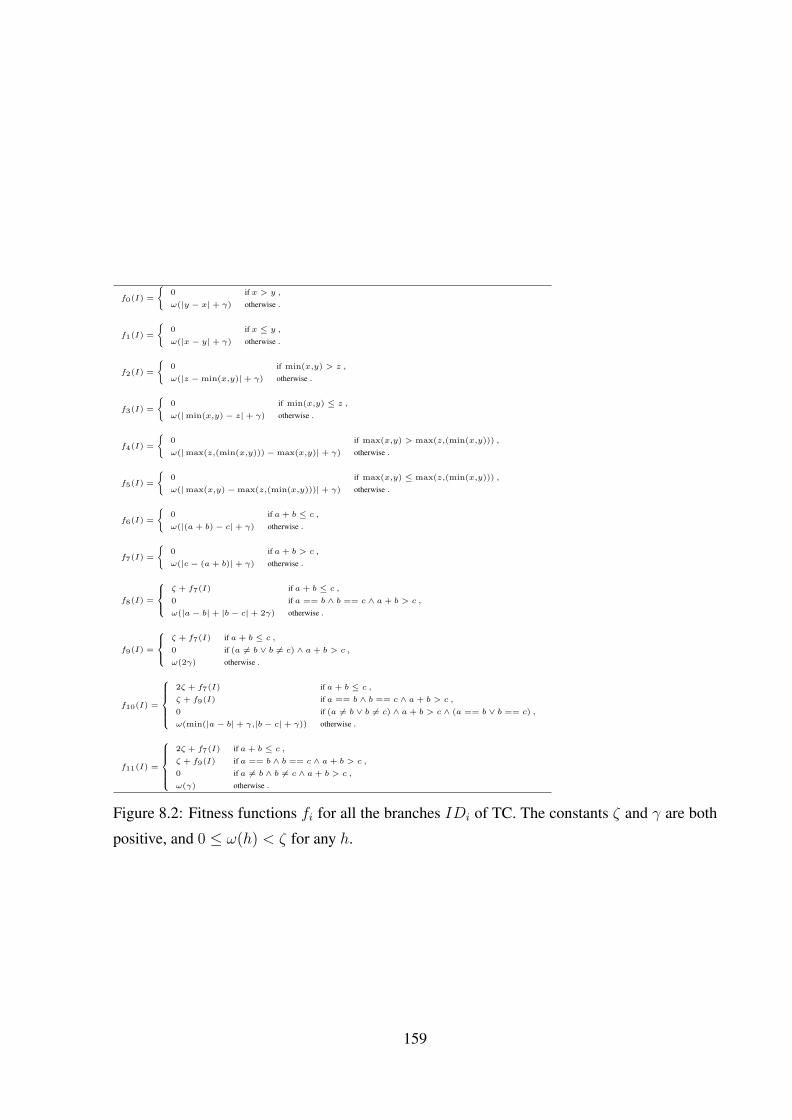
f0(I) =
(0 if x > y ,
ω(|y − x| + γ) otherwise .
f1(I) =
(0 if x ≤ y ,ω(|x− y| + γ) otherwise .
f2(I) =
(0 if min(x,y) > z ,
ω(|z −min(x,y)| + γ) otherwise .
f3(I) =
(0 if min(x,y) ≤ z ,ω(|min(x,y)− z| + γ) otherwise .
f4(I) =
(0 if max(x,y) > max(z,(min(x,y))) ,
ω(|max(z,(min(x,y)))−max(x,y)| + γ) otherwise .
f5(I) =
(0 if max(x,y) ≤ max(z,(min(x,y))) ,
ω(|max(x,y)−max(z,(min(x,y)))| + γ) otherwise .
f6(I) =
(0 if a + b ≤ c ,ω(|(a + b)− c| + γ) otherwise .
f7(I) =
(0 if a + b > c ,
ω(|c− (a + b)| + γ) otherwise .
f8(I) =
8><>:ζ + f7(I) if a + b ≤ c ,0 if a == b ∧ b == c ∧ a + b > c ,
ω(|a− b| + |b− c| + 2γ) otherwise .
f9(I) =
8><>:ζ + f7(I) if a + b ≤ c ,0 if (a 6= b ∨ b 6= c) ∧ a + b > c ,
ω(2γ) otherwise .
f10(I) =
8>>>><>>>>:2ζ + f7(I) if a + b ≤ c ,ζ + f9(I) if a == b ∧ b == c ∧ a + b > c ,
0 if (a 6= b ∨ b 6= c) ∧ a + b > c ∧ (a == b ∨ b == c) ,
ω(min(|a− b| + γ,|b− c| + γ)) otherwise .
f11(I) =
8>>>><>>>>:2ζ + f7(I) if a + b ≤ c ,ζ + f9(I) if a == b ∧ b == c ∧ a + b > c ,
0 if a 6= b ∧ b 6= c ∧ a + b > c ,
ω(γ) otherwise .
Figure 8.2: Fitness functions fi for all the branches IDi of TC. The constants ζ and γ are both
positive, and 0 ≤ ω(h) < ζ for any h.
159

while termination criterion not met
Choose I uniformly from S.
8.4.2 Hill Climbing
Given that the solution is a vector of integers (of length three in our particular case), an appro-
priate neighbourhood for solution Ii is the set of solutions:
Nd(Ii) := Ii + d | d ∈ D and Ii + d ∈ S ,
where D := (±1,0,0),(0,± 1,0),(0,0,± 1).A random restart is a common choice, and we use it for the HC that we analyse. Regarding
the strategy ψ, we do not need to define one. In fact, the following theoretical analyses of HC are
valid for all strategies satisfying the following constraint: unless a new better solution is found,
each neighbour solution will be visited in at most a constant number of iterations (assuming
that the neighbourhood size is constant). The implication is very straightforward: if the current
point Ii is neither a local or global optimum, then a better solution will be found in at most a
constant number of iterations. Note that this constraint is very common, and most of the HC
variants satisfy it. For the empirical study, we chose a simple strategy ψ that moves each time
to the first better solution it finds.
Definition 8.4.2 (Hill Climbing (HC)).
while termination criterion not met
Choose I uniformly at random from S.
while I not a local optimum in N(I),
Choose I ′ from N(I) according to strategy ψ
if f(I ′) < f(I), thenI := I ′.
8.4.3 Alternating Variable Method
In the employed AVM, small changes are done by adding ±1 to the integer input variables. The
bigger steps are done by doubling each time the current increment.
Definition 8.4.3 (Alternating Variable Method (AVM)).
160

while termination criterion not met
Choose I uniformly in S.
while I improved in last 3 loops
i := current loop index.
Choose Ti ∈ (1,0,0),(0,1,0),(0,0,1) such that
Ti 6= Ti−1 ∧ Ti 6= Ti−2.
found := true.
while foundfor d := 1 and d := −1
found := exploratory search(Ti,d,I).
if found, thenpattern search(Ti,d,I)
Definition 8.4.4 (exploratory search(Ti,d,I)).
I ′ := I + dTi.
if f(I ′) ≥ f(I), thenreturn false.
elseI := I ′.
return true.
Definition 8.4.5 (pattern search(Ti,d,I)).
k := 2.
I ′ := I + kdTi.
while f(I ′) < f(I)
I := I ′.
k := 2k.
I ′ := I + kdTi.
8.4.4 (1+1) Evolutionary Algorithm
Runtime analysis of evolutionary algorithms is difficult and only recently have rigorous results
become available. When initiating the analysis in a new problem domain, it is an important
161

first step to analyse a simple algorithm like the (1+1) EA. Without understanding the behaviour
of such a simple algorithm in the new domain, it is difficult to understand the behaviour of
more complex EAs, e.g. those EAs that use a population and crossover. Although the (1+1)
EA is relatively simple compared to other evolutionary algorithms, recent research has shown
that this algorithm is surprisingly efficient on a wide range of useful problems [28], including
sorting [282], minimum spanning tree [283] and Eulerian cycle [284].
Definition 8.4.6 ((1+1) EA).
Choose x uniformly from 0,1n.Repeat
x′ := x.
Flip each bit of x′ with probability 1/n.
If f(x′) ≥ f(x),
then x := x′.
8.4.5 Genetic Algorithms
In our analyses, we used a simple steady state implementation (SSGA) of GAs.
Definition 8.4.7 ((µ+1) Steady State Genetic Algorithm (SSGA)).
Sample a population P of µ points u.a.r. from S.
repeatwith probability pc(n),
Sample x and y u.a.r. from P .
(x′,y′) := one point crossover(x,y).
if maxf(x′),f(y′) ≥ maxf(x),f(y)then x := x′ and y := y′.
otherwiseSample x u.a.r. from P .
Flip each bit of x′ with probability 1/`(x′).
if f(x′) ≥ f(x)
then x := x′.
162

8.5 Empirical Study
Comparing theoretical analyses against empirical ones is useful to see which different types of
information they can give.
We ran each search algorithm on each branch of TC for the following values of n:
n ∈ 16,32,64,128,256,512,1024 .
For each size of n, we ran 30 trials (with different random seeds) and recorded the number of
fitness evaluations done before reaching a global optimum. We used the fitness functions in
Figure 8.2. We also ran experiments with only the approach level, i.e. without using the branch
distance.
Following [293], for each setting of algorithm and problem instance size, we fitted different
models to the observed runtimes using non-linear regression with the Gauss-Newton algorithm.
Each model corresponds to a one term expression ρ · t(n) of the runtime, where the model
parameter ρ corresponds to the constant to be estimated. The residual sum of squares of each
fitted model was calculated to identify the model which corresponds best with the observed
runtimes. This methodology was implemented in the statistical tool R [294]. Ten different
runtime models were considered (shown in Table 8.1). Note that the ten models were chosen
before the theoretical investigation was started, and that choice was made based on what we
thought would be appropriate.
The models with lowest error are shown in Table 8.2. The branch that seems most difficult
to cover is the one related to the classification as equilateral, i.e. ID8.
To study the effect that the size of data has on the accuracy of the models, we carried out an-
other set of experiments. We used a size set S = 16,32,64,128,256,512,1024,2048,4096,8192,and we run experiments with different ordered subsets of S (8 in total), as for example 16,32,64,. . . , 16, . . . ,8192. For each size in S we run 30 trials. Table 8.3 shows the results for branch
ID8. The fitness function uses the branch distance.
At any rate, this type of empirical analysis has the following limitations:
• Although more experimental data could lead to infer the right models, it is a priori dif-
ficult to estimate how much data is needed for obtaining them. Moreover, experiments
might be computationally expensive, hence it might be not possible to obtain the right
amount of data.
• If an algorithm has high complexity (e.g., Θ(2n) or Θ(n5)), only experiments with low
values of n can be carried out. This limits the accuracy of the model (e.g., there might be
163

Table 8.1: Models used for the non-linear regression. The constant ρ is the model parameter
that is estimated with the regression.
Runtime models
ρ · 1ρ · log(n)
ρ · log(n)2
ρ · nρ · n log(n)
ρ · n log(n)2
ρ · n2
ρ · n2 log(n)
ρ · n2 log(n)2
ρ · n3
not much difference between n5 and n4 log(n)2).
• When we try to fit a set of models, the correct one might not be necessarily among them.
8.6 Theoretical Analysis
For RS and AVM we studied the runtime on each target branch. For HM and (1+1) EA, we
only focused on branches ID8 and ID0. We have not formally analysed the runtime of SSGA,
although we carried out empirical experiments for sake of comparison.
For fitness function f8, in Figures 8.3 and 8.4 we show 3D graphs of the fitness landscape
with variable x fixed to n/4 and −n/4 respectively. The value of n is 24. Because the use of
a normalising function ω would make difficult to visualise the difference between the fitness
values of the solutions, we do not use a normalising function. Instead, to draw the fitness
landscape of f8 we use ω(h) = h, and then we choose ζ = 2n high enough to guarantee that
higher approach levels give worse fitness values. The value of γ is 1. Note that in Figure 8.3
there are small plateaus that correspond to the cases when a + b > c and the value of b is
modified.
164

Table 8.2: Result of the empirical study. Each branch has an ID based on its order in the code.
For each branch, there are shown the results whether the branch distance was used (T) or not
(F).
Branch ID Branch Distance RS HC AVM (1+1) EA (µ+1) SSGA
ID0 T 2.2000 0.9497 log(n)2 0.4558 log(n) 1.1470 log(n) 2.0480
F 2.2380 7.8480 8.0810 1.3270 log(n) 2.0520
ID1 T 1.9570 0.0173 n log(n) 0.5796 log(n) 5.5710 1.9050
F 1.8190 7.6380 0.9658 log(n) 1.0750 log(n) 1.9570
ID2 T 3.2140 0.0008 n2 1.1690 log(n) 10.6100 3.3430
F 3.2480 15.0100 12.6400 2.0560 log(n) 3.3950
ID3 T 1.4100 0.1435 n 0.4358 log(n) 3.5670 1.5330
F 1.5570 4.5140 0.5952 log(n) 0.5458 log(n) 1.4330
ID4 T 1.4860 0.0018 n log(n)2 0.4037 log(n) 0.5677 log(n) 1.5240
F 1.4430 4.2190 4.7520 3.8190 1.5330
ID5 T 0.3781 log(n) 0.0315 n log(n) 0.9759 log(n) 12.3300 3.1140
F 2.7480 14.1900 1.6010 log(n) 1.6730 log(n) 2.6670
ID6 T 1.0710 0.0126 n 1.2430 1.1240 1.0480
F 1.0810 1.2670 1.2430 0.1790 log(n) 1.0670
ID7 T 15.4000 0.9594 n 4.4670 log(n) 2.1370 log(n)2 30.5600
F 17.7400 95.5200 98.7700 10.6500 log(n) 48.9400
ID8 T 0.2476 n2 log(n) 1.3670 n 6.8240 log(n) 5364.0000 n 37.3000 log(n)2
F 2.4110 n2 0.0235 n2 log(n)2 1.7690 n2 0.0319 n2 log(n) 0.4475 n2
ID9 T 15.8300 0.1025 n log(n) 4.8760 log(n) 13.5100 log(n) 37.2200
F 14.2300 91.7200 93.7400 70.4400 40.9000
ID10 T 1.7310 n 1.1090 n 4.8320 log(n) 0.4556 n 5.6970 log(n)2
F 0.2525 n log(n) 3.8490 n 4.5880 n 3.4860 log(n)2 1.0800 n
ID11 T 17.5900 2.8810 n 31.8500 14.4700 log(n) 41.4700
F 19.1600 110.8000 105.6000 79.3500 45.8000
Table 8.3: Result of experiments for branch ID8. Data were collected with different values of
n.
Max n RS HC AVM (1+1) EA (µ+1) SSGA
16 1.8970 n log(n)2 1.8390 n 7.4300 log(n) 0.1839 n2 log(n) 3.9180 n log(n)
32 1.8970 n log(n)2 1.8390 n 7.4300 log(n) 0.1839 n2 log(n) 3.9180 n log(n)
64 0.0696 n2 log(n)2 1.6050 n 33.7400 0.1478 n3 21.3400 log(n)2
128 2.5960 n2 1.6400 n 6.5310 log(n) 0.2961 n2 log(n)2 24.5100 log(n)2
256 2.2170 n2 1.6680 n 6.2120 log(n) 14.1200 n2 10.3500 n
512 2.0150 n2 1.5510 n 6.3620 log(n) 57.4300 n log(n)2 35.0800 log(n)2
1024 1.9560 n2 1.5240 n 6.4170 log(n) 8.2890 n2 40.7100 log(n)2
2048 0.0218 n2 log(n)2 0.1559 n log(n) 6.6250 log(n) 682.0000 n log(n) 4.2890 n
4096 2.1580 n2 1.6950 n 6.9210 log(n) 6025.0000 n 0.0025 n2
8192 2.2910 n2 1.6920 n 7.2870 log(n) 6279.0000 n 116.7000 log(n)2
165

For branch ID8, when the branch distance is not used, the fitness function is:
f(I) =
2ζ if a+ b ≤ c ,
0 if a = b ∧ b = c ∧ a+ b > c, and
1ζ otherwise .
(8.1)
The proofs of the following theorems (plus some other minor theorems) can be found in
Appendix A.4.
Theorem 8.6.1. The expected time for RS to find an optimal solution to objective function f8 is
2n2 = Θ(n2) and for objective function f10 it is Θ(n). For all the other branches, the expected
time is Θ(1).
Theorem 8.6.2. The expected time for RS to find an optimal solution to objective function f8
when the branch distance is not used (i.e., Equation 8.1) is 2n2 = Θ(n2).
Theorem 8.6.3. The expected time for HC with neighbourhood Nd to find an optimal solution
to objective function f8 is Θ(n).
Theorem 8.6.4. The expected time for HC with neighbourhood Nd to find an optimal solution
to objective function f8 when the branch distance is not used (i.e., Equation 8.1) is Θ(n2).
Theorem 8.6.5. The expected time for HC with neighbourhood Nd to find an optimal solution
to objective function f0 is Θ(n).
Theorem 8.6.6. The expected time for AVM to find an optimal solution to any of the branches
of TC is O((log n)2).
Theorem 8.6.7. The probability that AVM has found an optimal solution to objective function
f8 within k · n · (log n)2 iterations is exponentially large 1− e−Ω(n), where k is a constant.
Theorem 8.6.8. The expected time for AVM to find an optimal solution to objective function f8
when the branch distance is not used (i.e., Equation 8.1) is Θ(n2).
Theorem 8.6.9. The expected running time of (1+1) EA on objective function f8 with integers
in the interval [0,n) represented in binary is Θ((log2 n)5).
Theorem 8.6.10. The expected runtime of (1+1) EA using either branch distance and approach
level (i.e. objective function f0), or only approach level with integers in the interval [0,n) on the
covering of branch ID0 is Θ(log2 n).
166

Var
iabl
e y
−10
−5
0
5
10
Variable z
−10−5
05
10
Transformed Fitness
0
20
40
60
Fitness Landscape for x=6
Figure 8.3: Fitness landscape of modified fitness function f8 with n = 24 and x fixed to the
value 6.
167

Var
iabl
e y
−10
−5
0
5
10
Variable z
−10−5
05
10
Transformed Fitness
0
20
40
60
Fitness Landscape for x=−6
Figure 8.4: Fitness landscape of modified fitness function f8 with n = 24 and x fixed to the
value −6.
168

8.7 Discussion
Table 8.4 summarises the empirical results and the theoretical ones for branches ID8 and ID0
(more details in Appendix A.4).
For branch ID8, the theoretical analyses show that RS has the worst runtime, whereas AVM
has the best. Not only can AVM find a solution in an efficient way, but we also proved that it has
an extremely low probability of not finding an optimal solution in a reasonable time (Theorem
8.6.7). In other words, it is very unlikely that AVM will run for a long time (depending on n)
without finding an optimal solution. This is an important result which cannot be obtained with
empirical studies. In fact, given any number k of experiments, we can say only little about the
worst case scenario, and how often it happens. For example, the experiments might show a low
runtime, although actually it can happen that with a small probability the runtime is enormous
(and hence in average the runtime is enormous), but k was not large enough to show it.
We proved that the runtime of AVM is O(log(n)2) on all the branches of TC (Theorem
8.6.6). This is necessary and sufficient to state that AVM has the best runtime among the anal-
ysed search algorithms because all the other heuristics have a strictly worse runtime on at least
one branch of TC.
It is not a surprise that AVM has the best runtime. The fitness landscape is relatively simple
even for the most difficult branch ID8. The big jumps of the pattern search quickly bring AVM
to a global optimum. AVM avoids the local optima that exist in this problem through restarts.
This is particularly helpful when the local optima are far from the global optima, as is the case
on this problem. Although the search landscape can be considered easy, analysing the actual
behaviour of search algorithms on this landscape is far from been trivial.
The empirical results in Table 8.3 show that, even with low values of n, most of the time the
correct runtimes for RS, HC and AVM are correctly inferred by the regression analysis. On the
other hand, the empirically estimated runtime for (1+1) EA in Table 8.3 is incorrect because the
correct model was not used for the regression.
We proved that (1+1) EA on target ID8 has a runtime of Θ((log n)5) (Theorem 8.6.9). That
was a surprise for us, because we were expecting something similar to the runtime of either
AVM or HC. Although the empirical results in Table 8.3 clearly show that (1+1) EA is much
slower than HC for low values of n, the asymptotic runtime of (1+1) EA is strictly better.
In other words, (1+1) EA is faster than HC for large values of n. If we do not consider the
constants, it will happen for values n for which n > (log n)5 is true, i.e. for n ≥ 5 · 106.
In our experiments we tested till n = 8192, and the performances of (1+1) EA for that value
169

(and below) are poor because (log 8192)5 = 371293, which is much higher than 8192. This is
a clear example of an algorithm that empirically seems to perform relatively poorly compared
with another algorithm, but actually has better scalability.
Because the first regression analysis on target ID8 did not include the correct runtime model
for (1+1) EA, supplemental regression analysis was carried out with the following large set of
models ρnt log(n)v, where t ∈ 0,1,2 and v ∈ 0, . . . ,10. The results are shown in Table 8.5.
Unfortunately, the correct model could still not be inferred from the empirical results. More
runs and empirical data is needed.
SSGA was not analysed theoretically. It would be difficult to estimate a runtime for this
algorithm based on the empirical results in Table 8.3. In fact, with size till 1024 the empirically
estimated runtime is ρ log(n)2, but if we add 30 new points obtained with size 2048, then the
inferred model is ρn. Adding another set of experiments (i.e., 30 points with size 4096) changes
the estimated model to ρn2, and then again to ρ log(n)2 when we consider size 8192. It is
unclear what model would be inferred with further empirical data on even larger instance sizes.
In general, we cannot answer this question with empirical studies, because for each tested size
there will be always a bigger one that we have not tested. Moreover, as was the case for (1+1)
EA, the correct runtime model may not be among those that were tested.
By Theorem 8.6.1, RS is very efficient (i.e., Θ(1)) for most of the branches. It is only for
ID8 that it gets the runtime Θ(n2). For branch ID10 it has the runtime Θ(n), which is equal with
the overall runtime of HC (assuming that HC has not worse runtime on the other 10 branches
besides ID0 and ID8 that we have not theoretically analysed). This is very important to keep
in mind. In fact, when we test software, not all of the testing tasks are necessarily difficult to
carry out. Some of them can be easy. We need sophisticated techniques only for the difficult
testing problems, because on simple problems they can give worse results. Because a priori it
is very difficult to understand whether a problem is either easy or difficult, hybrid strategies are
required. For example, doing random testing before applying more sophisticated techniques is
likely a wise choice.
Branch distance has been designed to improve the performance of search algorithms. When
we do not use the branch distance in the fitness function (e.g., as in Equation 8.1), the search
practically degenerates to random search. Counterintuitively, as we explained, on easy instances
that can even produce better results.
170

Table 8.4: Summary of the empirically (Emp.) and theoretically (Th.) obtained runtimes for
target branches ID8 and ID0. BD stands for “Branch Distance”.
Target Branch BD RS HC AVM (1+1) EA (µ+1) SSGA
Emp. Th. Emp. Th. Emp. Th. Emp. Th. Emp. Th.
ID8 T ρn2 log(n) Θ(n2) ρn Θ(n) ρ log(n) O(log(n)2) ρn Θ(log(n)5) ρ log(n)2 −F ρn2 Θ(n2) ρn2 log(n)2 Θ(n2) ρn2 Θ(n2) ρn2 log(n) − ρn2 −
ID0 T ρ Θ(1) ρ log(n)2 Θ(n) ρ log(n) Θ(log(n)) ρ log(n) Θ(log(n)) ρ −
Table 8.5: Result of experiments for branch target ID8 with a larger set of models. Data were
collected with different values of n.
Max n (1 + 1)EA
16 0.0120 log(n)7
32 0.0120 log(n)7
64 0.0000 n2 log(n)10
128 0.0023 n log(n)7
256 0.0009 log(n)10
512 0.0063 log(n)9
1024 0.0839 n log(n)5
2048 0.0716 log(n)8
4096 7.8240 log(n)6
8192 6279.0000 n
171

8.8 Conclusion
In this chapter we have illustrated how runtime analysis can be applied in SBSE, and we have
advocated its importance.
On one hand, it was shown that empirical results can be misleading. Theoretical analyses can
give insights into the behaviour of the search algorithms that empirical studies cannot give. This
insight can be very useful in the long term to design new algorithms that push the boundaries
of the current state of art. The obtained theoretical results are stronger than empirical ones.
They can be used in the future any time the analysed case study is employed in new empirical
analyses where novel techniques are validated and compared.
On the other hand, theoretical analyses have their own limits. It can be hard to analyse the
runtime, and it might be infeasible to show for large and complex software (e.g., it is required
that all the optima are known in advance). Besides, proofs for a particular testing problem are
difficult to generalise to another case study. Theoretical analyses are hence not meant to replace
empirical studies.
It is important to note that theoretical analyses are not meant to be used on new problems
for which we are looking for a solution. Their goal is to get insight knowledge and to compare
the behaviour of search algorithms. This is similar to the type of empirical analysis in which
different search algorithms are applied (and then compared) to known problems whose optimal
solutions have been already found (e.g., [115]).
In future work, we are planning to formally analyse more search algorithms that are com-
monly used in SBSE, like for example SA and GAs. This can be very challenging, but their the-
oretical analyses in traditional combinatorial problems are appearing in recent years [28]. Other
problems in SBSE (e.g., requirement engineering [32]) should be addressed as well. Regarding
software testing, general theoretical results that can be applied to entire classes of software are
worth pursuing.
172

Chapter 9
Conclusion
This chapter concludes this thesis with an overview of the achieved results in Section 9.1. Plans
for future work are described in Section 9.2.
9.1 Summary of Contributions
In this thesis we have proposed a novel co-evolutionary framework to tackle software engineer-
ing problems in which source code needs to be either generated or modified (Chapter 4). We
instantiated our conceptual framework in three different tools aimed to three different software
engineering problems, namely Automatic Refinement (Chapter 5), Automatic Fault Correction
(Chapter 6) and Automatic Improvement of Execution Time (Chapter 7).
In this thesis we have shown that our approach is able to obtain promising results in all of
these tasks. However, its application in complex real-world applications likely requires more
research to improve the performance. Furthermore, writing software tools to manipulate real-
world programming languages is a very time consuming and challenging task.
Automatic Refinement is the most difficult task among the ones we analysed. Only simple
programs were able to be evolved. However, in the other two tasks the source code of the input
program can be exploited to guide the search to more promising areas instead of starting the
search from random programs. This is the reason why stronger results are obtained.
The three analysed tasks share some common properties. Our conceptual framework high-
lights these properties, such that optimisations aimed to improve the performance can be directly
applied to all of these tasks.
In the case of Automatic Refinement, techniques exist in literature to address it. However,
they can be applied only when the gap between formal specifications and programs is not wide,
173
i.e. a direct mapping from formal specification to code should exist. Although the obtained
results of our tool are still limited to small programs, our approach overcomes that limitation.
In literature, there are some few techniques to address the task of repairing software au-
tomatically. Our contribution has been to show how to use search algorithms in this context.
Search algorithms have been effective in many different tasks, and in this thesis we have shown
that they are useful as well in the task of repairing software automatically. The use of search al-
gorithms is particularly appropriate for this task because the search space of possible programs
is infinite and exhaustive approaches are unfeasible.
Regarding the optimisation of non-functional criteria like for example execution time, we
are aware of no work in literature on optimising programs at their source code level. Compilers
use a large set of different optimisation techniques, but they are not able yet to improve poor
algorithmic choices. They cannot restructure the entire source code in a more efficient way.
On one hand, in our experiments with our novel framework we obtained optimisations of the
source code that current compilers like GCC are not able to produce yet. On the other hand, our
approach does not guarantee that the obtained optimised source code is semantically equivalent.
Therefore, our framework should be used to understand how source code can be improved, but
it should not be used without a human analysis of its output.
Other important contribution of this thesis is a first theoretical runtime analysis for search
based software testing (Chapter 8). Theoretical analyses are important to understand why search
heuristics are successful on a particular class of problems. A better understanding of how search
algorithms work help to get a better insight knowledge of the addressed problem. The long term
goal is to exploit this knowledge to design and choose better tailored algorithms. The field of
search based software engineering is still missing of theoretical analyses (i.e., apart from our
work we are aware only of [25, 26, 27]). These types of results are more difficult to obtain, but
they are stronger than empirical results. For example, different search algorithms can scale up
in a different way. In Chapter 8 we gave a non-trivial example of a search algorithm that seems
to perform poorly, but it actually scales up better (i.e., for bigger instances its performance is
better). The point is that it would be very difficult to show it with empirical analyses, that
because better performance in that case is obtained only for very large instances.
Software testing is a very important and expensive task in the development of software, and
it is one of the main components of our novel framework. Search algorithms have been applied
with successful results in software testing [19]. In this thesis we also give the contribution of
analysing several different search algorithms applied to test data generation for object-oriented
software (Chapter 3). In particular, we analysed the role that is played by the length of the test
174

sequences. Although this property of the problem is quite important, it has received only little
attention in literature.
9.2 Future Work
The novel framework presented in this thesis is composed of many different components that
interact in a non-trivial way. There is hence a large set of possible improvements that can be
studied. Here we just summarise the main research directions that can be followed:
• Although the framework can be employed to address different software engineering prob-
lems, better results can be obtained when domain knowledge is exploited. This means that
each of these software engineering problems has some unique properties that need to be
exploited to obtain better results. For example, on one hand different seeding strategies
based on the source code of the input program can be designed for automatic software
repair. On the other hand, in automatic refinement there would be no input program.
• An evolved program that is able to pass a set of test cases is not guaranteed to be correct.
Our confidence in its correctness is hence based on the quality of used test cases during
the evolutionary process. When we employ co-evolution, the choice of how we evolve
the test cases is hence crucial for the final outcome. In this thesis we just consider some
simple strategies to choose the test cases (e.g., branch coverage). More sophisticated
strategies should be designed and evaluated.
• The field of search based software engineering is lacking of theoretical foundations. Al-
though in this thesis we give first runtime analyses in software testing, this is just a first
step. Much more research is required. For example, it is important to understand which
are the classes of problems for which search algorithms are efficient and which are the
classes for which they are inefficient. Explaining why that happens would help in the long
run to design more sophisticated and tailored algorithms with better performance.
175

Appendix A
A.1 Formal Proofs for Chapter 3
Theorem 3.7.1. If R(l) 6= ∅, |G(l)| > 0 and |C(k)| = c (where c is a positive constant c > 1)
for all k ≥ l, then r(k + 1) > r(k) for all k ≥ l.
Proof. For all the global optima in G(l), adding a function call at the end of the sequence does
not change the fact that they are global optima. Therefore, |G(l + 1)| ≥ |G(l)| · |M | · c.Let choose z among the global optima G(l) such that:
• z(j − 1) is not a global optimum, whereas z(j) is a an optimal solution.
• All function calls after position j belong to the set R(l).
At least one element z of this type exists, because given any global optimum we can just
replace all the function calls (one at the time) with a new one belonging to R(l) until the new
considered sequence is still optimal.
A new sequence z′ generated from z by replacing in position j a new function call of type
R(l) is not a global optimum. And it will be necessarily different from the |G(l)| · |M | · coptima we described before. At this sequence z′, if we append the function call we removed
from position j, then this new sequence is necessarily a global optimum. The number of global
optima is hence at least |G(l + 1)| ≥ |G(l)| · |M | · c+ |R(l)|. Therefore:
r(l + 1) = |G(l+1)||S(l+1)|
≥ |G(l)|·|M |·c+|R(l)||M |l+1·cl+1
= |G(l)||M |l·cl + |R(l)|
|M |l+1·cl+1
= |G(l)||S(l)| + |R(l)|
|S(l+1)|
= r(l) + |R(l)||S(l+1)|
> r(l)
176

Once proved r(l + 1) > r(l), to conclude the proof we can simply use induction to prove
r(k + 1) > r(k), this because |G(k)| ≥ |G(l)| > 0.
Theorem 3.7.2. If |G(l)| > 0 and |C(k + 1)| > |C(k)| for all k ≥ l, then it is not necessarily
true that r(k + 1) > r(k) with k ≥ l.
Proof. We just need to find one case for which r(k + 1) ≤ r(k). Let |C(l + 1)| = c + t where
c = |C(l)| and t > 0. In the infinite space of possible programs, let consider one for which
the use of one of any of these t new inputs makes impossible to cover the target branch. The
non-optimal solutions W (l + 1) for length l + 1 are hence at least:
|W (l + 1)| ≥ |S(l + 1)| − (|M |l+1 · cl+1) . (A.1)
This is a very low underestimation of their number, but it is more than enough to prove this
theorem.
To have r(l + 1) > r(l), we need enough global optima such that |G(l + 1)| > |S(l + 1)| ·(|G(l)|/|S(l)|). Because |S(l+ 1)| = |G(l+ 1)|+ |W (l+ 1)|, then we would not have enough
global optima if |W (l+1)| > |S(l+1)|−(|S(l+1)| ·(|G(l)|/|S(l)|)). Therefore, by Inequality
A.1, we just need to prove:
|S(l + 1)| − (|M |l+1 · cl+1) > |S(l + 1)| −(|S(l + 1)| · |G(l)|
|S(l)|
),
which can be reduced to:
1− 1
(1 + tc)(l+1)
>(
1− |G(l)||S(l)|
).
The previous inequality is clearly true for t → ∞, but could be false for small values of t
like for example t = 1. Because the conditions of the theorem just state |C(k + 1)| > |C(k)|,we hence need to analyse the smallest case t = 1. For t > 1 we can just follow the same type
of reasoning. Instead of analysing the case r(l + 1) < r(l), let study the case r(l + z) < r(l).
Because t = 1 (i.e., |C(l + 1)| = |C(l)| + 1), then for the same type of discussion done for
Inequality A.1, we have:
|W (l + z)| ≥ |S(l + z)| − (|M |l+z · cl+z) ,
this because |C(l+ z)| = |C(l)|+ z (it easily follows from |C(l+ 1)| = |C(l)|+ 1). We would
not have enough global optima to guarantee r(l + z) > r(l) if:
|S(l + z)| − (|M |l+z · cl+z) > |S(l + z)| −(|S(l + z)| · |G(l)|
|S(l)|
),
177

(seq (write_result (array 0 ))
(loop 0 length
(if (bigger_or_equal read_result (array index))
skip
(write_result (array index )))))
Figure A.1: Implementation of MaxValue defined in Figure 5.3.
(seq (write_result 1 )
(loop 0 length
(if (equal (array 0 )(array index ))
skip
(write_result 0 ))))
Figure A.2: Implementation of AllEqual defined in Figure 5.4.
which can be reduced to:
1− 1
(1 + zc)(l+z)
>(
1− |G(l)||S(l)|
).
Again, this inequality is clearly true for z → ∞. For proving this theorem we do not need to
calculate the smallest value z for which this inequality is true. Therefore, because it does exist
at least one value z for which r(l+z) < r(l), there would be necessarily one intermediate value
l ≤ k < l + z for which r(k + 1) < r(k).
A.2 Implementation of the Specifications used in Chapter 5
The following figures from A.1 to A.1 show correct implementations of the formal specifications
of the programs used in the case study in Chapter 5.
A.3 Formal Proofs for Chapter 6
Lemma A.3.1. Let t be the number of nodes (in the syntax tree) that are related to faults. Let s
be the number of nodes that are given the same rank as these t nodes, whereas l is the number of
nodes that have lower rank and h is the number of nodes that have higher rank. The probability
178

(if (bigger_or_equal input_0 (add input_1 input_2))
(write_result 1)
(if (bigger_or_equal input_1 (add input_0 input_2))
(write_result 1)
(if (bigger_or_equal input_2
(add input_0 input_1))
(write_result 1)
(if (and (equal input_0 input_1)
(equal input_1 input_2))
(write_result 4)
(if (or (or (equal input_0 input_1)
(equal input_1 input_2))
(equal input_0 input_2))
(write_result 3)
(write_result 2))))))
Figure A.3: Implementation of TriangleClassification defined in Figure 5.5.
(seq (seq (write_result (array input_0))
(write_array input_0 (array input_1)))
(write_array input_1 read_result))
Figure A.4: Implementation of Swap defined in Figure 5.6.
(if (bigger (array input_0) (array input_1))
(seq (seq (write_result (array input_0))
(write_array input_0 (array input_1)))
(write_array input_1 read_result)) skip )
Figure A.5: Implementation of Order defined in Figure 5.7.
179

(loop 0 length
(loop 0 (sub length 1)
(if (bigger (array input_0) (array input_1))
(seq (seq (write_result (array input_0))
(write_array input_0 (array input_1)))
(write_array input_1 read_result))
skip )))
Figure A.6: Implementation of Sorting defined in Figure 5.8.
(seq (loop 0 length
(loop 0 (sub length 1)
(if (bigger (array input_0) (array input_1))
(seq (seq (write_result (array input_0))
(write_array input_0
(array input_1)))
(write_array input_1
read_result))
skip )))
(write_result (array (div (sub length 1 )2 ))))
Figure A.7: Implementation of Median defined in Figure 5.9.
180

δ(n) of choosing one of the t faulty nodes using a tournament of size n is given by Equation 6.4.
Proof. Given a tournament of n nodes, let ζ be the number of faulty nodes (that are t in total)
in n. Let γ be the number of non-faulty nodes in n that have higher rank than ζ (they are h in
total) and let ψ the number of nodes with the same rank as ζ .
We need to pick up at least one of the t nodes and none of the h nodes (i.e., P (γ = 0)P (ζ ≥1 | γ = 0)). Then, among these n nodes, the probability of choosing a faulty node depends on
how many of the s nodes are in these n (i.e., P = ζ/(ζ +ψ)). The probability of γ = 0 is equal
to not picking up any of the h nodes for n times:
P (γ = 0) =(
1− h
l + s+ t+ h
)n.
The probability of ζ ≥ 1 is equal to 1 minus the probability of having ζ = 0. We are
assuming γ = 0, hence:
P (ζ ≥ 1 | γ = 0) = 1−(
1− t
l + s+ t
)nFor any possible values of ζ and ψ, P (ζ = i ∧ ψ = j | ζ ≥ 1 ∧ γ = 0) is the probability
they assume the values i and j respectively. Therefore, we pick up one of the ζ nodes with the
following probability:
K(n) =n∑i=1
n−i∑j=0
(( i
i+ j
)P (ζ = i ∧ ψ = j | ζ ≥ 1 ∧ γ = 0)
).
Calculating this probability P (ζ = i∧ψ = j | ζ ≥ 1∧γ = 0) requires some more passages.
Let’s consider:
T =t
l + s+ t,
S =s
l + s+ t,
L =l
l + s+ t.
Without considering their permutations, we have that the probability of having a set of size
n with ζ = i ∧ ψ = j ∧ γ = 0 is:
Z(i,j) = T iSjLn−i−j .
Using Bayes’ theorem, we obtain:
181

Z(i,j | i ≥ 1) =(Z(i,j)− Z(i,j | i = 0)(L+ S)n
)/(1− (L+ S)n) .
Because we use Z to calculate K(n), and because in K(n) the value i is always different
from 0, we have:
Z(i,j | i = 0)(L+ S)n = 0 ,
and therefore:
Z(i,j | i ≥ 1) =Z(i,j)
(1− (L+ S)n)=
T iSjLn−i−j
(1− (L+ S)n)=
ln−i−jsjti
(l + s+ t)n − (l + s)n.
We still need to calculate the possible permutations of the n nodes, and these are(ni
)(n−ij
).
Therefore:
P (ζ = i ∧ ψ = j | ζ ≥ 1 ∧ γ = 0) =
(n
i
)(n− ij
)ln−i−jsjti
(l + s+ t)n − (l + s)n.
Finally:
δ(n) = P (γ = 0)P (ζ ≥ 1 | γ = 0)∑n
i=1
∑n−ij=0
((ii+j
)P (ζ = i ∧ ψ = j | ζ ≥ 1 ∧ γ = 0)
)
=(
1−(
1− tl+s+t
)n)(1− h
l+s+t+h
)n∑ni=1
∑n−ij=0
((ii+j
)(ni
)(n−ij
)(ln−i−jsjti
(l+s+t)n−(l+s)n
)).
A.4 Formal Proofs for Chapter 8
A.4.1 Global Optima
For each branch IDi, we calculate the number of global optima.
Proposition A.4.1. For the objective function f0, considering the space of solutions S, there
are g0 = (1/2)(n− 1)n2 global optima.
Proof. We need to consider all the cases in which x > y and z can assume any value.
g0 = n
(n−1)∑i=1
(n− i) = n(n(n− 1)− (1/2)(n− 1)(n)
)= (1/2)(n− 1)n2 .
182

Proposition A.4.2. For the objective function f1, considering the space of solutions S, there
are g1 = (1/2)(n+ 1)n2 global optima.
Proof. If branch ID0 is not executed, then ID1 is executed. Therefore, using Proposition A.4.1:
g1 = n3 − (1/2)(n− 1)n2 = (1/2)(n+ 1)n2 .
Proposition A.4.3. For the objective function f2, considering the space of solutions S, there
are g2 = (1/6)(n− 1)(n)(2n− 1) global optima.
Proof. We need to consider all the cases in which x > z and y > z.
g2 =n−1∑i=1
(n− i)2 = (1/6)(n− 1)(n)(2n− 1) .
Proposition A.4.4. For the objective function f3, considering the space of solutions S, there
are g3 = (1/6)(n)(n+ 1)(4n− 1) global optima.
Proof. If branch ID2 is not executed, then ID3 is executed. Therefore, using Proposition A.4.3:
g3 = n3 − (1/6)(n− 1)(n)(2n− 1) = (1/6)(n)(n+ 1)(4n− 1) .
Proposition A.4.5. For the objective function f4, considering the space of solutions S, there
are g4 = (1/3)(n)(n− 1)(2n− 1) global optima.
Proof. We need to consider all the cases in which max(x,y) > max(z,min(x,y)). There is no
valid solution to this inequality if x = y. Because max(x,y) ≥ min(x,y), those cases can be
simplified to max(x,y) > z with x 6= y.
g4 = 2n−1∑i=1
n∑j=i+1
(j−1) = 2n−1∑i=1
((1/2)(n)(n−1)−(1/2)(i)(i−1)
)= (1/3)(n)(n−1)(2n−1) .
Proposition A.4.6. For the objective function f5, considering the space of solutions S, there
are g5 = (1/3)(n)(n2 + 3n− 1) global optima.
183

Proof. If branch ID4 is not executed, then ID5 is executed. Therefore, using Proposition A.4.5:
g5 = n3 − (1/3)(n)(n− 1)(2n− 1) = (1/3)(n)(n2 + 3n− 1) .
Proposition A.4.7. For the objective function f8, considering the space of solutions S, there
are n/2 global optima, and they are of the form G = (t,t,t), with t > 0.
Proof. This can be proved by considering fitness function f8, in which the minimal fitness
value is given for (a + b > c) ∧ (a = b) ∧ (b = c). The points G are the only that satisfy
(a = b) ∧ (b = c), and t + t > t implies t > 0. Because the range of the variables is
R = −n/2 + 1, . . . ,n/2, there are g8 = n/2 possible different t with t > 0.
Proposition A.4.8. For the objective function f10, considering the space of solutions S, there
are g10 = (3/16)(n)(3n− 8) global optima.
Proof. We first analyse the case b = c.
k =
(3
1
) n/2∑a=1
((n/2)− a) = (3/2)(n)
n/2∑a=1
1− 3
n/2∑a=1
a = (3/8)(n)(n− 2) .
We then need to consider the cases in which a = b.
t =
(3
1
)( n/2∑a=1
min(2a−1,n/2)∑c=a+1
1)
= 3( n/4∑a=1
2a−1∑c=a+1
1)
+ 3( n/2∑a=1+n/4
n/2∑c=a+1
1)
= (3/16)(n2 − 4n) .
Finally:
g10 = k + t = (3/8)(n)(n− 2) + (3/16)(n2 − 4n) = (3/16)(n)(3n− 8) .
Proposition A.4.9. For the objective function f11, considering the space of solutions S, there
are g11 = (1/16)(n)(n− 4)(n− 5) global optima.
Proof. We need to consider all the cases in which a 6= b 6= c and a+ b > c. To make this latter
predicate true we need a ≥ 2.
g11 = 3!(∑(n/2)−2
a=2
∑(n/2)−1b=a+1
∑min(a+b−1,n/2)c=b+1 1
)= 6
(∑(n/4)−1a=2
∑(n/2)−ab=a+1
∑a+b−1c=b+1 1
)+ 6(∑n/4
a=2
∑(n/2)−1b=(n/2)−a+1(n/2)− b
)+
+6(∑(n/2)−2
a=(n/4)+1
∑(n/2)−1b=a+1 (n/2)− b
)= (1/32)(n)(n− 4)(n− 8) + (1/64)(n)(n+ 4)(n− 4) + (1/64)(n)(n2 − 12n+ 32)
= (1/16)(n)(n− 4)(n− 5) .
184

Proposition A.4.10. For the objective function f9, considering the space of solutions S, there
are g9 = (1/16)(n)(n+ 2)(n− 2)global optima.
Proof. Using Propositions A.4.8 and A.4.9, we just need to add the global optima for branches
ID10 and ID11.
g9 = (3/16)(n)(3n− 8) + (1/16)(n)(n− 4)(n− 5) = (1/16)(n)(n+ 2)(n− 2) .
Proposition A.4.11. For the objective function f7, considering the space of solutions S, there
are g7 = (1/16)(n)(n2 + 4) global optima.
Proof. Using Propositions A.4.7 and A.4.10, we just need to add the global optima for branches
ID8 and ID9.
g9 = (n/2) + (1/16)(n)(n+ 2)(n− 2) = (1/16)(n)(n2 + 4) .
Proposition A.4.12. For the objective function f6, considering the space of solutions S, there
are g6 = (1/16)(n)(15n2 − 4) global optima.
Proof. If branch ID7 is not executed, then ID6 is executed. Therefore, using Proposition
A.4.11:
g6 = n3 − (1/16)(n)(n2 + 4) = (1/16)(n)(15n2 − 4) .
A.4.2 General Properties
The following simple properties of the problem will be used extensively in the runtime analysis.
Proposition A.4.13. For the objective function f8, let a ≤ b ≤ c, and v > 0, then f8(a,b,c) <
f8(a− v,b,c).
Proof. In the case when a+b ≤ c, then a−v+b ≤ c and we have f8(a,b,c) = ζ+ω(c−a−b+γ)
and f8(a− v,b,c) = ζ + ω(c− (a− v)− b+ γ), in which case the proposition holds. Assume
on the other hand that a+ b > c. Let g be:
g =
0 if a = b ∧ b = c ,
2γ if a 6= b ∧ b 6= c ,
γ otherwise ,
185

we get:f8(a− v,b,c) ≥ ω(c− a+ v + g)
> ω(c− a+ g)
= f8(a,b,c) .
Proposition A.4.14. For objective function f8, if a ≤ b ≤ c, and v > 0, then f8(a,b,c) <
f8(a,b,c+ v).
Proof. In the case when a+ b ≤ c, we have:
f8(a,b,c+ v) = ζ + ω(v + c− a− b+ γ)
> ζ + ω(c− a− b+ γ)
= f8(a,b,c) .
For the opposite case a+ b > c, we have:
f8(a,b,c+ v) ≥ ω(v + c− a+ g)
> ω(c− a+ g)
= f8(a,b,c) ,
where g is as defined in the proof of Proposition A.4.13.
Proposition A.4.15. Given x and y uniformly and independently distributed in R, then their
expected difference with y ≥ x is E[y − x|y ≥ x] = n−13
= Θ(n). The largest difference would
be y − x = n− 1 = Θ(n)
Proof.E [y − x | y ≥ x] = (n+ 2(n− 1) + 3(n− 2) + . . .+ n(1))
/ n(n+1)2− 1
=∑n
i=0(i+ 1)(n− i) · 2n(n+1)
− 1
= n(n+1)(n+2)6
· 2n(n+1)
− 1
= n−13
= Θ(n) .
The highest value that y can take is n/2. The lowest value x can take is −n/2 + 1. Hence,
n/2− (−n/2 + 1) = n− 1.
Proposition A.4.16. The expected difference between c and a is linear in n independently of b,
i.e. E [c− a] = (n+1)2
= Θ(n).
186

Proof. The expected value of a is E [a | b] = b/2−(n/2+1)/2, whereas E [c | b] = b+(n/2−b)/2. It now follows that E [c− a | b] = E [c | b]− E [a | b] = (n+ 1)/2, independently of b.
Proposition A.4.17. Given x and y uniformly and independently distributed in R, then the
probability that x > y is (1/2)− (1/2n). The probability that x ≤ y is (1/2) + (1/2n).
Proof. The probability that x > y, with X and Y the random variables representing them, is:
Pr [X > Y ] =∑y
n/2∑i=y+1
Pr [X = i | Y = y] · Pr [Y = y]
=1
2− 1
2n,
The probability of x ≤ y is hence 1− (12− 1
2n) = 1
2+ 1
2n
Lemma A.4.1. For search algorithms that use the fitness function only for direct comparisons
of candidate solutions, the expected time for covering a branch IDw is not higher than the
expected time to cover any of its nested branches IDz.
Proof. Before a target nested branch IDz is executed, its “parent” branch IDw needs to be
executed. Until IDw is not executed, the fitness function fwz (i.e., search for IDz and IDw is not
covered) will be based on the predicate of the branch IDw. Hence, that fitness function would
be equivalent to the one fw used for a direct search for IDw. In particular, fwz (I) = ζ + fw(I),
this because the approach level would be different. However, because the constant ζ > 0 would
be the same to all the search points, the behaviour of a search algorithm, that uses the fitness
function only for direct comparisons of candidate solutions, would be same on these two fitness
functions (all search algorithms used in Chapter 8 satisfy this constraint).
Because the time to solve (i.e., finding an input that minimises) fwz is not higher than the
time needed for fz and because fwz is equivalent to fw, then solving fw cannot take in average
more time than solving fz.
A.4.3 Analysis of RS
Lemma A.4.2. Given g global optima in a search space of |S| elements, then the expected time
for RS to find an optimal solution is E[TRS] = |S|/g.
187

Proof. The probability of sampling an optimal solution is p = g/|S|. The behaviour of RS can
therefore be described as a Bernoulli process, where the probability of getting a global optimum
for the first time after t steps is geometrically distributed Pr [TRS = t] = (1−p)t−1 · (p). Hence,
the expected time for RS to find a global optimum is E[TRS] = (1/p) = |S|/g.
Theorem 8.6.1. The expected time for RS to find an optimal solution to objective function f8 is
2n2 = Θ(n2) and for objective function f10 it is Θ(n). For all the other branches, the expected
time is Θ(1).
Proof. The search space is composed of n3 elements. The proof simply follows by Lemma
A.4.2 and all the Propositions in Section A.4.1.
Theorem A.4.1. The probability that RS has found an optimal solution to objective function f8
within n3 iterations is exponentially large 1− e−Ω(n).
Proof. Using the inequality (1−1/x)x ≤ e−1 and Theorem 8.6.1, we can see that Pr [TRS > n3] =((1− 1
2n2
)2n2)n/2
≤ e−n/2.
Theorem 8.6.2. The expected time for RS to find an optimal solution to objective function f8
when the branch distance is not used (i.e., Equation 8.1) is 2n2 = Θ(n2).
Proof. RS does not exploit any gradient in the fitness function. Therefore, the use of the branch
distance does not make any difference. Proof hence follows from Theorem 8.6.1.
A.4.4 Analysis of HC
Theorem 8.6.3. The expected time for HC with neighbourhood Nd to find an optimal solution
to objective function f8 is Θ(n).
Proof. We first need to prove that all the points of the form L = (t,t,t) with t ≤ 0 are local
optima. Because a+b ≤ c holds for all of them, we have f8(L) = ζ+ω(−t+γ). Any operation
on the vector I can either increase c by one, or decrease a by one. In both the cases, the resulting
points L′ have worse fitness (Proposition A.4.13 and A.4.14), that is f8(L′) = ζ+ω(−t+1+γ).
Because f8(L′) > f8(L), the points L are local optima.
Considering Propositions A.4.13 and A.4.14, a solution I ′ is not accepted if the value of a
has decreased, or if the value of c has increased. Moreover, there is always a gradient for a to
increase up to b, and for c to decrease down to b, because there would be a fitness improvement
whether a + b ≤ c is true or not. Although the value of b can either increase or decrease,
188

its number of changes is finite, because a ≤ b ≤ c is always true and because HC accepts
as new solutions only strictly better points. Therefore, after a finite number of steps (i.e., the
algorithms does not enter in an infinite loop, like it would happen if new solutions with equal
fitness would be accepted), the current solution I converges to a point of the form W = (t,t,t),
with a ≤ t ≤ c. If b does not change during the search, then t = b.
Although we have already proved that all the points on the form (t,t,t) are either local or
global optima, only after the discussion in the previous paragraph we can state that L are the
only possible local optima. In fact, regardless of the starting point, HC reaches either L or G,
and G are global optima by Proposition A.4.7.
A step is called successful if the new search point I ′ is accepted. The number of successful
steps η for HC to reach an optimum depends on how the value of b changes. If it does not
change, then there are b − a steps in which a increases, and c − b steps in which c decreases.
Hence, η = c− a. There is only one case in which b can decrease: (a + b > c) ∧ (b = a + 1),
because in all other cases the fitness would never be better. If b is decreased before a increases
(that depends on how the strategy ψ works), then η = 1 + c− a, because then a = b and a and
b cannot be changed again. If it is still (a + b > c) but (b 6= a + 1), then b cannot be altered
until a is increased up to b− 1, because the fitness would not change. On the other hand, while
(a + b ≤ c), there is always a gradient for b to increase up to c − a + 1. However, if a ≤ 0, b
can increase up to c. Again, depending on ψ, it is possible that c decreases before b increases,
and vice-versa. In the worst case with a = b and a ≤ 0, we can have η = 2(c − a), because b
can take c − a steps to increase up to c, and other c − a steps for a to increase up to c as well.
Therefore, regardless of the starting point I and strategy ψ, the number η of successful steps is
bounded by (c− a) ≤ η ≤ 2(c− a).
Unless the algorithm is stuck in an optimum, in at most a constant number of iterations
it will find a better solution in its neighbourhood. Considering the bounds of η, the expected
number of iterations for reaching an optimum is Θ(c−a). For Proposition A.4.16, starting from
a random point the expected number of iterations for reaching either a local or a global optimum
is hence Θ(n).
When an optimum is reached, HC does a restart if that point is a local optimum. Therefore,
we need to calculate the number of restarts that are required for HC to find an optimal solution.
If c ≤ 0, then HC is bound to reach a local optimum regardless of the strategy ψ. This
happens because it will reach a point (t,t,t) with t ≤ c. Because c ≤ 0 implies t ≤ 0, then that
point is a local optimum. With the same type of reasoning, if a > 0, then HC is bound to find a
global optimum. We said that there is only one case in which b can decrease up to a, and that is
189

b = a+ 1. However, because for doing it there is the need of a+ b > c, then a > 0 is required.
Therefore, if b > 0, then b will always remain a positive value. Hence, we can generalise the
condition of reaching a global optimum from a > 0 to a more significant b > 0. Note that a > 0
implies b > 0, but the opposite is not always true.
There is still to consider the case (b ≤ 0)∧ (c > 0), in which the result is actually depending
on the strategy ψ. If it chooses to decrease c at least down to 0 before increasing b up to 1, then
a local optimum will be reached, or a global optimum if it chooses to do the opposite. However,
as we will show, the analysis of that situation is not important for finding a lower and an upper
bound for the number of required restarts.
The probability of starting from a point with c ≤ 0 is Pr [c ≤ 0] = 18. On the other hand, the
probability of starting from a point with b > 0 is equivalent to the probability of flipping a coin
three times and getting at least two heads, hence, Pr [b > 0] = 18+31
8= 1
2. Therefore, regardless
of the strategy ψ, we have that the probability of reaching a global optimum from a random point
is 12≤ Pr [global] ≤ 3
4, whereas for reaching a local optimum it is 1
8≤ Pr [local] ≤ 1
2.
Therefore, the expected number of restarts is no more than 2. Because reaching either a
local or global optimum from a random point requires Θ(n) steps, and the expected number of
restarts to reach a global optimum is no more than 2, it follows that the expected runtime of HC
is on TC Θ(n).
Theorem A.4.2. The probability that HC with neighbourhoodNd has found an optimal solution
to objective function f8 within k · n2 iterations is exponentially large 1 − e−Ω(n), where k is a
constant.
Proof. The time to reach a local optimum is at most k · n iterations, where the constant k is
determined by the strategy ψ. The probability that HC finds a local optimum more than n times
before a global optimum is found is less than 2−n = e−Ω(n).
Theorem 8.6.4. The expected time for HC with neighbourhood Nd to find an optimal solution
to objective function f8 when the branch distance is not used (i.e., Equation 8.1) is Θ(n2).
Proof. Objective function in Equation 8.1 can assume only 3 values. Hence, before doing a
restart, there can be at most 2 successful steps. Because the neighbourhood size is constant,
then there can be at most a constant number of steps before doing a restart.
On the one hand, in the optimal scenario, all the solutions that are 2 steps away from a global
optimum would have a gradient toward it. The probability of starting from one of these points
would be n2· 62 · 1
n3 = 18n2 , hence the runtime would be Ω(n2). On the other hand, in the worst
190

scenario none of these points have a gradient, and HC would degenerate in a RS with runtime
O(n2) (Theorem 8.6.1). Because the lower bound is equal to the upper bound, hence HC has
runtime Θ(n2).
Theorem 8.6.5. The expected time for HC with neighbourhood Nd to find an optimal solution
to objective function f0 is Θ(n).
Proof. Following by Proposition A.4.17, we have 14≤ Pr [x > y] < 1
2for any n > 1. Hence,
with constantly bounded probability, HC finds a solution in the first step, i.e. Θ(1) steps.
In the case in which x ≤ y, there is a gradient to either increase x or to decrease y. By
Proposition A.4.15, the distance is Θ(n), hence Θ(n) steps are required.
Considering the constant bounds on the probability of the 2 different runtimes, the overall
runtime is Θ(n).
A.4.5 Analysis of AVM
Lemma A.4.3. For any branch, if the probability that the random starting point is a global
optimum is lower bounded by a positive constant p > 0, then AVM needs at most a constant
number Θ(1) of restarts to find a global optimum.
Proof. If we consider only the starting point, the AVM behaves as a random search, in which the
probability of finding a global optimum is bigger than p. That can be described as a Bernoulli
process (see Lemma A.4.2), with expected number of restarts that is lower or equal than 1/p.
Theorem A.4.3. The expected time for AVM to find an optimal solution to the coverage of
branches ID0 and ID1 is O(log n).
Proof. Considering that the search is done for values of n bigger or equal than 8, then both the
searches for ID0 and ID1 start with a random point that is a global optimum with a probability
lower bounded by a positive constant (Proposition A.4.17). Therefore, AVM needs at most a
constant number of restarts (Lemma A.4.3), independently of the presence and number of local
optima.
For both branches, either the starting point is a global optimum, or the search will be in-
fluenced by the distance x − y that is Θ(n) (Proposition A.4.15). We hence analyse this latter
case.
191

Until the predicate is not satisfied, the fitness function ω(|y − x| + γ) (with γ a positive
constant) based on the branch distance rewards any reduction of that distance. The third variable
z does not influence the fitness function, hence an exploratory search fails on that. For the
coverage of ID0, the variable x has gradient to increase its value, and y has gradient to decrease.
For ID1 it is the opposite. The distance |x − y| can be covered in O(log n) steps of a pattern
search.
Theorem A.4.4. The expected time for AVM to find an optimal solution to the coverage of
branches ID2, ID3, ID4 and ID5 is O(log n).
Proof. The sentences in lines 5, 8 and 11 of the source code (Figure 8.1) only swap the value of
the three input variables. Hence, the predicate conditions of branches ID2, ID3, ID4 and ID5
are directly based on the values of two different input variables.
The type of predicates is the same of branches ID0 and ID1 (i.e.,>), and the condition of the
comparison is the same (i.e., > on two input variables). The three input variables are uniformly
and independently distributed in R, and by Proposition A.4.15 the maximum distance among
them is Θ(n). There are the same conditions of Theorem A.4.3 apart from the fact that the
variables could be swapped during the search, i.e. the fact that lines 5 and 8 are executed or not
can vary during the search.
For branches ID2 and ID3, starting from z no variation of the executed code is done until
the branch is covered. For branch ID3, for either x or y a search starting from the maximum
of them would result in no improvement of the fitness function. The minimum of x and y has
a gradient to decrease, and while it does so the relation of their order is not changed. Hence,
no variation of the executed code is done. On the other hand, for branch ID2, the minimum
has gradient to increase, but the pattern search would stop once it becomes the maximum of the
two (e.g., x > y if the search started on x with x < y). That happens in at most O(log n) steps
because their difference is at most Θ(n) (Proposition A.4.15). If the next variable considered by
AVM is not z, then the above behaviour will happen again. However, the next variable will be
necessarily z, hence we have at most O(log n) steps done 3 times, that still results in O(log n)
steps.
For any pair of values we have that min(x,y) ≤ max(x,y). For branch ID4, if it is not
executed, then max(x,y) ≤ max(z,min(x,y)) and necessarily it would be z ≥ max(x,y) ≥min(x,y). Hence, z would have gradient to decrease down until max(x,y), in which case ID4
gets executed after O(log n) steps. A modification of the minimum value between x and y does
192

not change the fitness value. For the maximum value, it can increase up to z, in which case ID4
gets executed after O(log n) steps. The relation of the order of the input variables would not
changed during those searches.
For branch ID5, if it is not executed, then max(x,y) > max(z,min(x,y)) and necessarily
it would be x 6= y and max(x,y) > z. Starting the search from the maximum of x and y would
have gradient to decrease down to max(z,min(x,y)), that would be done in O(log n) steps that
will make ID5 executed. If z < min(x,y), modifying z would have no effect to the fitness
function, whereas the minimum of x and y has gradient to increase up to max(x,y). In the
other case z ≥ min(x,y), it is the other way round, i.e. z can increase whereas the minimum
between x and y cannot change. In both cases, in O(log n) steps branch ID5 gets executed with
no change in the relation of the order of the input variables.
The expected time for branches ID2, ID3, ID4 and ID5 is therefore the same as for
branches ID0 and ID1, i.e. O(log n).
Theorem A.4.5. The expected time for AVM to find an optimal solution to the coverage of
branch ID6 is O(log n).
Proof. If the predicate a + b ≤ c is not true, the fitness function would be ω(|a + b − c| + γ)
(with γ a positive constant). For values a ≤ 0, the predicate is true because a+ b ≤ b ≤ c.
There is gradient to decrease a and b, and there is gradient to increase c. If the search starts
from either a or b, in O(log n) steps of a pattern search the target variable assumes a negative
value (the highest possible starting value is n/2). In particular, if the search starts from b, at a
certain point the input variable representing b will instead represent a. Otherwise, it sufficient
to increase c up to the value a + b ≤ n/2 + n/2 = n, that can be done in O(log n) steps of a
pattern search.
Lemma A.4.4. For objective f8, given a starting point (a,b,c), before doing a restart AVM
converges to an optimum T = (t,t,t), where a ≤ t ≤ c.
Proof. The variable representing a can only increase (Proposition A.4.13), and it has a gradient
to increase up to b, i.e., each succession of increments of a has better fitness till a′ = b. Similarly,
c cannot increase (Proposition A.4.14), and it has a gradient to decrease down to b, and although
b can change, b will still be in the interval [a,c].
193

b0 b1 b2 b3c0
Figure A.8: Example where c0 − b0 = 15, in which case bs = c0.
In the case of a pattern search that leads to a value k outside [a,c], then that value has a
gradient toward a if k < a and toward c if k > c (that can be easily proved with an induction on
Propositions A.4.13 and A.4.14).
AVM modifies the same variable until it finds better solutions. Hence, before any other
variables is modified, the current variable will have a value in the interval [a,c].
Because, AVM accepts only strictly better solutions and it is deterministic, it will hence
converge to a point T = (t,t,t) in a finite number of iterations.
Lemma A.4.5. For objective f8, starting an exploratory search on any variable g ∈ x,y,z,after Θ(log(n)) steps of AVM the distance of g from the closest other variable is reduced by at
least 2/3.
Proof. The variable representing a can only increase (Proposition A.4.13) toward b, and the
variable representing c can only decrease down to b (Proposition A.4.14).
Considering the fitness function f8, the variable representing b can increase toward c if
a+ b ≤ c. Otherwise, it can be modified only in 2 cases:
b = a+ 1 ,
b = c− 1 .
In these two cases, a single exploratory search makes either a = b or b = c in at most two steps.
If g represents either a or b, then a pattern search will increase its value, otherwise the value
will be decreased (case c).
Let h be the closest variable to g. After a pattern search, we can have three cases: either
g = h, or g < h or g > h. Given (a0,b0,c0) the ordered values of (x,y,z) when AVM starts
to do a new exploratory search, Figures A.8, A.9 and A.10 show examples of these three cases
for g representing b. For Propositions A.4.13 and A.4.14, a pattern search ends when g assumes
value bigger than c or lower than a.
To simplify the proof, assume that g < h (the other case g > h can be analysed in the same
way by inverting the signs of the arithmetic operations and the inequalities).
Let g′ be the value of g at the end of the pattern search. For Proposition A.4.16, it follows
194

b0b1 b2 b3c0bs bs+1
Figure A.9: Example where c0 − b0 = 17, in which case bs+1 is not accepted, as indicated by
the dashed arrow.
b0b1 b2 b3c0bs bs+1
Figure A.10: Example where c0 − b0 = 25, in which case bs+1 is accepted.
that |g − h| = Θ(n). Hence, given s the number of steps for which AVM gets g as close as
possible to h with gs < h, then s = Θ(log(n)).
After s steps, the increment to the variable g is∑s
i=0 2i = 2s+1 − 1. Let k = 2s+1, hence
after s steps the value of g is gs = g + k − 1. Hence:g + k − 1 < h ,
g + 2k − 1 > h .
There can be two cases: either g′ = gs, and that happens if gs+1 leads to a worse fitness, or
otherwise g′ = gs+1. On the one hand, for g′ = gs, then it should be that:
h− gs ≤ gs+1 − h ,
which is the case for k ≥ 23(h− g + 1). On the other hand, for g′ = gs+1 it should be:
h− gs > gs+1 − h ,
and the highest value that g′ can have is gs+1 = g + 43(h − g + 1). Therefore it follows that
|h− g′| ≤ 13|h− g|.
Lemma A.4.6. The lower and upper bounds of the expected time of AVM for converging to an
optimum for objective f8 is Ω(log n) and O((log n)2).
Proof. By Lemma A.4.4, AVM converges to a solution T = (t,t,t) before doing a restart if T is
not a global optimum.
Starting the search on any variable g ∈ x,y,z, after Θ(log(n)) steps, its distance from
the closest other variable is reduced by at least 2/3 (Lemma A.4.5). AVM does modifications
195

b0c0c1cs
cs+1
Figure A.11: Example in which c0 − b0 = 6. In that case cs+1 is accepted. To note that is
the continuation of the search done in figure A.10, which is represented in dotted arrows. The
former bs+1 has become the new c0, whereas the old c0 is now the new b0.
on the same variable till improvements can be found. Figure A.11 shows an example of a new
pattern search on the same variable.
By applying Lemma A.4.5 recursively, because the distance is reduced at least by 2/3 at
each pattern search, then after O(log n) pattern searches we have g that is equal to another
variable, which we call h. Therefore, that in expectation would happen after a number of steps
with bounds Ω(log n) and O((log n)2).
However, the distance |g − h| gets reduced at each search. Hence, the upper bound for the
steps is: ∑logni=0 log( n
3i) =
∑logni=0 (log n+ log 3−i)
= (log n)2 − log 3∑logn
i=0 i
= (log n)2 − log 3 (logn)(logn+1)2
= O((log n)2) .
Although the distance is reduced at each new pattern search, the upper bound does not
change.
Once we get g = h, any modification of g and h would not lead to any better value for
fitness function f8. The modification of the third variable will follow the same behaviour of g,
and after another i expected iterations with same bounds, AVM converges to T . Because only
a constant number of variables is modified (i.e., 2), the lower and upper bounds of the expected
time of AVM for converging to T is Ω(log n) and O((log n)2).
Lemma A.4.7. For objective f8, in expectation, AVM needs a constant number Θ(1) of restarts
to reach a global optimum.
Proof. If a > 0, then AVM converges to an optimum (Lemma A.4.4) which is global (Proposi-
tion A.4.7). The probability of this event is 18. Considering restarts as a geometric process, the
expected number of restarts is less or equal to 8 (Lemma A.4.3).
196

Theorem A.4.6. The lower and upper bounds of the expected time of AVM to find an optimal
solution to objective f8 is Ω(log n) and O((log n)2).
Proof. By Lemma A.4.7 there are Θ(1) restarts, and by Lemma A.4.6, each search requires in
expectation Ω(log n) and O((log n)2) steps regardless it takes to a global or local optimum.
Theorem 8.6.7. The probability that AVM has found an optimal solution to objective function
f8 within k · n · (log n)2 iterations is exponentially large 1− e−Ω(n), where k is a constant.
Proof. Except for the choice of search point in the initial iteration, or in case of a restart, AVM
is a deterministic algorithm. By Lemma A.4.6, AVM has reached a local optimum within k ·(log n)2 iterations, for some constant k. A global optimum is found if the initial search point
satisfies a > 0, an event which occurs with constant probability p. The probability that AVM
needs more than n restarts before the initial search point satisfies the condition above, is less
than (1− p)n = e−Ω(n).
Theorem 8.6.8. The expected time for AVM to find an optimal solution to objective function f8
when the branch distance is not used (i.e., Equation 8.1) is Θ(n2).
Proof. The proof follows the same discussion as in the proof of Theorem 8.6.4 for HC. The
difference is that the visited neighbourhood might be larger due to a possible pattern search.
However, the number of visited solutions is still bounded by a constant, so the runtime is like
the one of HC, i.e. Θ(n2).
Theorem A.4.7. The expected time for AVM to find an optimal solution to the coverage of
branch ID7 is O((log n)2).
Proof. The branch ID8 is nested to branch ID7, hence by Lemma A.4.1 and Theorem A.4.6
the expected time is O((log n)2).
Theorem A.4.8. The expected time for AVM to find an optimal solution to the coverage of
branch ID9 is O((log n)2).
Proof. By Theorem A.4.7, the branch ID7 can be covered in O((log n)2) steps. The branch
ID9 (that is nested to ID7), will be covered if ¬(a = b ∧ b = c). If that predicate is not true, a
single exploratory search of AVM makes it true because it is just sufficient to either increase or
decease any input variable by 1. The only case in which this is not possible is for I = (1,1,1),
because it is the only solution that satisfies a = b∧b = c∧a−1+b ≤ c∧a+b ≤ c+1∧a+b > c.
In that case, a restart is done.
197

With a probability that is lower bounded by a constant, in a random starting point each input
variable is higher than n/4. In that case, a + b > c, because (n/4) + 1 + (n/4) + 1 > (n/2).
By Lemma A.4.3, we need only Θ(1) restarts.
Theorem A.4.9. The expected time for AVM to find an optimal solution to the coverage of
branch ID10 is O((log n)2).
Proof. By Theorem A.4.8, the branch ID9 can be covered in O((log n)2) steps. The branch
ID10 (that is nested to ID9), will be covered if only two input variables are equal (and not all
three equal to each other at the same time).
If when the branch ID7 (branch ID9 is nested to it) is executed all the three input variables
are equal (in that case branch ID8 is executed), then a single exploratory search is sufficient to
execute branch ID10, because we just need to change the value of a single variable.
The other case in which all the three variables are different is quite complex to analyse.
Instead of analysing it directly, we prove the runtime by a comparison with the behaviour of
AVM on the branch ID8 (proved in Theorem A.4.6).
Once branch ID9 is executed, the fitness function f10 for covering branch ID10 is based on
min(δ(a = b),δ(b = c)), whit δ the branch distance function for the predicates. For simplicity,
let consider δ(a = b) < δ(b = c). The other case can be studied in the same way.
An exploratory search cannot accept a reduction of the distance c− b, because the value of
f10 would not improve. A search on a would leave the distance c− b unchanged. About b, only
a decrease of its value would be accepted, and in that case the distance c− b would increase (but
that has no effect on the fitness function because it takes the minimum of the two distances).
Because the branch distance δ only rewards the reduction of the distance b−a, a search starting
from either a or b will end in a = b by modifying only the value of only one of these variables
(AVM keeps doing searches on the same variable till an exploratory search fails). During that
search, the fitness function would hence be based on δ(a = b).
In a search for covering branch ID8, if the branch ID7 (in which both ID8 and ID10 are
nested) is executed, then the fitness function f8 depends on δ(a = b) + δ(b = c). A search
starting from a would finish in a = b for the same reasons explained before or it would finish in
a′ > b (with a′ the latest accepted point for a that will become the new b in the next exploratory
search). During that search, the value of δ(b = c) does not change, so it can be considered as a
constant. Because AVM uses the fitness function only on direct comparisons, the presence of a
constant does not influence its behaviour. Therefore, in this particular context (i.e., δ(a = b) <
198

δ(b = c), branch ID7 executed and search starting from a) the behaviour of AVM on f10 and f8
will be the same until a = b or a′ > b.
In the case a = b, branch ID10 gets executed and the search for that branch ends. In the
other case a′ > b, the previous b becomes the new ak and a′ becomes the new bk. Modifications
on the variable c does not change the value of either ak or bk. The previous analysis can hence
be recursively applied to the new values ak and bk. If a′ > c, then ak = b, bk = c, ck = a′ and it
will become the case δ(a = b) > δ(b = c).
It is still necessary to analyse the behaviour of AVM on f10 when the search starts on b
rather than a. That is similar to the case of f8 when the variable c is decreased down to b. In that
context, the two fitness functions are of the same type because in f8 the distance δ(a = b) would
be a constant until b = c or c′ < b (with c′ the latest accepted point for c that will become the
new b in the next exploratory search). Therefore, the runtime for AVM on f10 to obtain a = b
would be the same.
By Theorem A.4.6, the expected time for covering branch ID8 is O((log n)2). Because we
proved that the coverage of ID8 takes more time than the coverage of ID10, then the expected
runtime for covering ID10 is O((log n)2).
Theorem A.4.10. The expected time for AVM to find an optimal solution to the coverage of
branch ID11 is O((log n)2).
Proof. By Theorem A.4.8, the branch ID9 can be covered in O((log n)2) steps. The branch
ID11 (that is nested to ID9), will be covered if a 6= b ∧ a 6= c ∧ b 6= c. In the moment that the
branch ID9 is executed, then the three variables cannot assume all the same value (otherwise
the branch ID8 would have been executed). If that predicate is not true, a single exploratory
search of AVM makes it true because it is just sufficient to increase by 1 any of the two variables
that have same values.
Theorem 8.6.6. The expected time for AVM to find an optimal solution to any of the branches
of TC is O((log n)2).
Proof. The proof follows from Theorems A.4.3, A.4.4, A.4.5, A.4.7, A.4.6, A.4.8, A.4.9 and
A.4.10.
199

A.4.6 Analysis of (1+1) EA
In1 contrast to the other algorithms we have analysed so far, the (1+1) EA uses binary strings
to represent solutions. We denote the ith bit of bitstring x by xi, the length of a bitstring x by
`(x), and the concatenation of two bitstrings x and y either by x · y or xy. Test cases for the
triangle classification program will be encoded as bitstrings I ∈ 0,13m, which for notational
convenience will be denoted as a triple x,y,z where x := I1 · · · Im, y := Im+1 · · · I2m and
z := I2m+1 · · · I3m. Here, we will consider unsigned integers, where a bitstring x of length `(x)
has integer value bin(x) :=∑`(x)
i=1 xi · 2m−i.The (1+1) EA is a comparison-based algorithm in the sense that the decision whether to
replace the current search point x with a new search point x′ only depends on the ordering of x
and x′ with respect to the fitness function f , and not on the actual fitness value of search point x′.
Hence, the (1+1) EA will not change behaviour if the fitness function f is replaced by another
fitness function g where for all bitstrings x and y, f(x) < f(y) if and only if g(x) < g(y).
To simplify the notation, we will therefore use the function f(x,y,z) = |x − y| + |y − z| =
maxx,y,z − minx,y,z instead of function f8. Furthermore, instead of directly analysing
function f0, we consider the function f(x,y) = y − x.
To analyse the progress of the (1+1) EA towards the optimum of function f8, we define the
block length of a search point, and use this is a potential function.
Definition A.4.1 (Block length). Let x,y and z be three bitstrings of length m with longest
common prefix σ. The prefix-length of the triple x,y,z is the length `(σ) of the prefix σ, and the
block length is the largest integer s such that x,y,z ∈ σ10sα,σ01sβ | α,β ∈ 0,1m−`(σ)−1−s.
Among bitstrings with the same prefix length, the value of Korel’s distance function de-
creases almost monotonically with the block length.
Lemma A.4.8. On objective function f8, if bitstrings x,y and z have length m, longest common
prefix σ, and block length s, then 2r−s + 1 ≤ f(x,y,z) ≤ 2r−s+2 − 1, where r = m− `(σ)− 2.
Proof. The initial part of the triangle classification program assigns the minimal value of x,y,z
to variable a, and the maximal value of x,y,z to c. Hence, we have f(x,y,z) = bin(c)− bin(a).
If the bitstring representations of a and c can be written on the form a = σ01sxβ and b =
σ10s1α, then bin(σ10s1α) − bin(σ01sxβ) = 2r−s · (3 − x) + bin(α) − bin(β). Otherwise,
it must be possible to write the bitstrings on the forms c = σ10s1α and a = σ01sxβ, in
which case bin(σ10sxα) − bin(σ01s0β) = 2r−s · (2 + x) + bin(α) − bin(β). Furthermore,
1The theorems on (1+1) EA were proved by Dr. Per Kristian Lehre. They are here included for sake of clarity.
200

the difference bin(α) − bin(β) is at least −2r−s + 1 and at most 2r−s − 1. So in all cases,
2r−s + 1 ≤ bin(c)− bin(a) ≤ 2r−s+2 − 1.
The probability of increasing the prefix-length is small.
Lemma A.4.9. Consider (1+1) EA on objective function f8 with bitstring length 3m. If the
prefix-length of the current search point is s, then the probability that the current search point
in the following iteration has prefix length s + i for any i > 0, is less than m−l−1, where
l := mini,s.
Proof. The case where i > s is trivial, because one of the bitstrings differs in s + 1 positions,
and it is therefore necessary to flip at least these s+ 1 bits to increase the length of the common
prefix bits by i.
Consider the case where i ≤ s. Without loss of generality, assume that the current search
point is of the form σ10i−100s−iα,σ01i−111s−iβ,σ01i−111s−iκ, where `(α) = `(β) = `(κ) =
m − `(σ) − s − 1. By Lemma A.4.8, the fitness value of this search point is no more than
2`(α)+1 − 1. To increase the prefix-length by i, it is necessary to flip at least i bits after σ
in at least one of the bitstrings. Assume that the mutated search point is accepted without
also flipping the next bit in position `(σ) + i + 1. Then the search point will be of the form
σ01i−10α′,σ01i−11β′,σ01i−11κ′, where `(α′) = `(β′) = `(κ′) = m−`(σ)−i−1 ≥ `(α). The
fitness of this search point is at least bin(σ01i−11β′)− bin(σ01i−10α′) ≥ 2 · 2`(α′) − bin(α′) ≥2`(α
′) +1, which is strictly larger than the original search point and therefore contradicts that the
search point was accepted by (1+1) EA.
We are now in position to lower bound the runtime of (1+1) EA on the equilateral branch of
the triangle inequality program. We only count the runs where the algorithm reaches the search
point 10m−1,01m−1,01m−1 before the optimum has been found, and optimistically assume
that all other runs are finished in 0 iterations.
Lemma A.4.10. With constant probability p > 0, (1+1) EA will reach a search point on the
form 10m−1,01m−1,01m−1 before reaching the global optimum of objective function f8.
Proof. With probability 3/29, the initial search point is on the form x,y,z = 100α,011β,011κ.Clearly, this search point does not satisfy the predicate (a + b <= c), hence the remaining
of the search consists in trying to reach the equilateral branch. Let the block length of this
search point be s ≥ 2. The probability that the prefix length increases, is by Lemma A.4.9 no
more than 1/m2. In the following, we will analyse a duration of km2 iterations, where k will be
201

s0 s1 s2 s3 s4 s5 s6
q q q q q
p p p p p p
1− p 1− p− q1− p− q1− p− q1− p− q1− p− q 1
Figure A.12: Markov chain in the proof of Lemma A.4.10.
specified later, and assume that the prefix length will never increase during this period, an event
which happens with probability at least (1− 1/m2)km2
= Ω(1).
By Lemma A.4.8, if the block length increases to s + 2, then all future search points will
have block length at least s + 1. We call a trial a sequence of search points where the current
block length s is increased or decreased. The trial lasts until either the block length has been
reduced to s− 1, or the block length has been increased from s to s+ 2, in which case the trial
is called successful. We now estimate the probability of a successful trial.
In order to decrease the block length to s − 1, it is necessary to flip at least one of the bits
in position 1 + s of x, y or z, an event which happens with probability no more than 1/m. In
order to increase the block length to s + 2, it suffices to flip the two right-most 1-bits in α, the
two right-most 0-bits in β and the two right-most 0-bits in κ. Each of these 6 bit-flips happen
with a probability of 1/3m in any iteration. When all 6 bits have been flipped, the block length
must necessarily have been increased to at least s+ 2. To analyse the stochastic process behind
these bitflips, we construct a Markov chain corresponding to the number of those bits that have
the “correct” value. We pessimistically assume that at most one bit can be flipped correctly in
each iteration, and if the block length is reduced, or one of these bits are flipped back, then
all bits are lost. The Markov chain is depicted in Figure A.12, where state si corresponds to
i correct bits, and the values of the variables occurring in the state transition probabilities are
defined as p := 1/3em and q := 1/m. With some algebraic manipulation, it is easy to see that
the expected hitting time from state s0 to state s6 is 7/p + 6q/p2 = km for some constant k.
The block length must be increased at most m times, hence the expected time until the search
point is on the form 10m−1,01m−1,01m−1 is no more than km2, and by Markov’s inequality,
the probability that this search point is reached within 2km2 steps is at least 1/2.
The probability of increasing the block length within km2 iterations is by union bound
no more than k. Hence, the probability that the search point 10m−1,01m−1,01m−1 has been
obtained before the prefix length is increased is at least 3/29 · (1/2)/(1/2 + k) > 0.
202

Theorem A.4.11. The expected running time of (1+1) EA on objective function f8 with integers
in the interval [0,n) represented in binary is Ω((log2 n)5).
Proof. Define m := log2 n. We define a typical run as a run where the EA reaches the search
point 10m−1,01m−1,01m−1, which has function value 1, before reaching the global optimum.
By Lemma A.4.10, there is a constant probability that the run is typical. We will lower bound
the expected runtime by the expected number of iterations needed to find the global optimum
starting from this position. By Lemma A.4.8, the only non-optimal search points that will be
accepted from this point are on one of the forms σ10s,σ01s,σ01s and σ01s,σ10s,σ10s. All
other search points have block lengths at most m − `(σ) − 2, and therefore function values at
least 2.
In order to reach the global optimum, it is necessary to increase the prefix length to m. We
use drift analysis [266] to bound expected runtime until this happens, using m minus the prefix
length as distance function. In order to decrease the distance by i > 0, it necessary to flip at
least i+ 3 bits simultaneously. Hence, the expectation of the drift ∆ in each iteration is at most∑mi=1 i · m−i−3 = O(m−4). The initial distance from the optimum is B = Θ(m), hence the
expected runtime is at least B/E [∆] = Ω(m5).
Theorem A.4.12. The expected running time of (1+1) EA on objective function f8 with integers
in the interval [0,n) represented in binary is O((log2 n)5).
Proof. Define m := log2 n. We divide a run of the EA into three phases. The first phase begins
with the initial iteration and lasts until a+ b > c holds. The second phase ends when the search
point has block length m − `(σ) − 1. The third phase lasts until a search point a = b = c, i.e.
the global optimum, has been found.
For the first phase to end, it suffices to wait for a search point on the form a = 1α,b =
1β,c = 1κ, because bin(1α)− bin(1β)− bin(1κ) ≤ −1 for any α,β and κ. Such search points
are obtained by flipping at most 3 bits simultaneously, hence the expected duration of the first
phase is bounded by O(m3).
The runtime of the second phase can be analysed using drift analysis, similarly to the proof
of Lemma A.4.10. Hence, the duration of the second phase is bounded from above by O(m2).
For the third phase, we apply drift analysis as in the proof of Theorem A.4.11. For reasons
that will be explained later, we start analysing the algorithm after iteration m3. In the worst
case, the search point has prefix-length 0 at this point in time. In a given iteration, we distinguish
between two complementary events. Let E be the event that the search point is on one of the two
forms σ1 ·10s,σ1 ·01s,σ1 ·01s or σ0 ·10s,σ0 ·10s,σ0 ·01s, and let the complementary event
203

E denote the event that the search point is on one of the two forms σ0 · 10s,σ0 · 01s,σ0 · 01sor σ1 · 10s,σ1 · 10s,σ1 · 01s.
In the case of event E , it is necessary to flip 5 bits to reduce the prefix-length by 1. Hence,
the conditional expected drift becomes E [∆ | E ] = Ω(m−4) − O(m−5) = Ω(m−4). In the
complementary event E , it is necessary to flip 4 bits to reduce the prefix length by 1, but the
probability of increasing the prefix-length is no larger than the probability of increasing the
prefix-length. Hence, we have E[∆ | E
]≥ 0. We first claim that Pr [E ] = Ω(1). If this claim
holds, we have unconditional expected drift E [∆] = Ω(m−4), and the expected duration of the
second phase is O(m5).
We finally show that the claim Pr [E ] = Ω(1) holds. Let the current iteration number be
t. Let random variable X ∈ 0,1 denote the value of the last bit of the common prefix σ
in iteration t. We will analyse the behaviour of variable X in the time interval t − m3 to t
conditional on the event F that the prefix length is constant in this period. The probability of
increasing the prefix-length in any iteration is less than m−4, so the probability of event F is at
least (1−m−4)m3
= Ω(1). Given that the prefix length is constant, the probability of changing
the value of X in any iteration is Θ(m−3). If X0 = 0, then the probability that Xm3 = 1 is at
least m3 · (1−m−3)m3−1m−3 = Ω(1). If X0 = 1, then the probability that Xm3 = 1 is at least
m3 · (1−m−3)m3
= Ω(1). Hence, the probability of event E is Ω(1).
The expected duration of all three phases is therefore O(m5).
Theorem 8.6.9. The expected running time of (1+1) EA on objective function f8 with integers
in the interval [0,n) represented in binary is Θ((log2 n)5).
Proof. The proof follows from Theorems A.4.11 and A.4.12.
We now turn to the runtime of (1+1) EA on the first branch in the program ID0, in which
case Korel’s distance function gives the minimisation objective y − x.
Theorem 8.6.10. The expected runtime of (1+1) EA using either branch distance and approach
level (i.e. objective function f0), or only approach level with integers in the interval [0,n) on the
covering of branch ID0 is Θ(log2 n).
Proof. Define m := log2 n. We will focus on the leading bits of x and y only. For the upper
bound, we pessimistically assume that the predicate cannot be satisfied when x1 = 0 and y1 = 0,
however it is clear that the predicate is necessarily satisfied when y1 = 0 and x1 = 1. In the
worst case, we start with y1 = 1 and x1 = 0. From this state, it suffices to wait for a sequence
of two bit-flips which do not flip the same variable twice. The expected time until one bit-flip
204

occurs is less than em, and the expected time until the right bit-flip sequence occurs is no more
than 8em.
For the lower bound, we note that there is a constant probability that the initial search point
has y1 = 1 and x1 = 0, and that the probability that none of these are flipped withinm iterations
is at least (1− 2/m)m = Ω(1). Hence, the runtime is lower bounded by Ω(m).
Note that the previous theorems for (1+1) EA do not consider negative values for the three
input variables. In order to consider negative values, it is necessary to extend the runtime analy-
sis of (1+1) EA. However we conjecture that if signed integers are represented using a separate
sign bit, the asymptotic runtime results will be the same.
205

Bibliography
[1] A. Arcuri, P. K. Lehre, and X. Yao. Theoretical runtime analyses of search algorithms on
the test data generation for the triangle classification problem. In International Workshop
on Search-Based Software Testing (SBST), pages 161–169, 2008.
[2] A. Arcuri and X. Yao. Search based software testing of object-oriented containers. In-
formation Sciences, 178(15):3075–3095, 2008.
[3] A. Arcuri. Theoretical analysis of local search in software testing. In Symposium on
Stochastic Algorithms, Foundations and Applications (SAGA), 2009. (to appear).
[4] A. Arcuri. Insight knowledge in search based software testing. In Genetic and Evolu-
tionary Computation Conference (GECCO), pages 1649–1656, 2009.
[5] A. Arcuri. Full theoretical runtime analysis of alternating variable method on the triangle
classification problem. In International Symposium on Search Based Software Engineer-
ing (SSBSE), pages 113–121, 2009.
[6] A. Arcuri. On search based software evolution. In International Symposium on Search
Based Software Engineering (SSBSE), pages 39–42, 2009.
[7] A. Arcuri, D. R. White, J. Clark, and Xin Yao. Multi-objective improvement of soft-
ware using co-evolution and smart seeding. In International Conference on Simulated
Evolution And Learning (SEAL), pages 61–70, 2008.
[8] A. Arcuri and X. Yao. A novel co-evolutionary approach to automatic software bug
fixing. In IEEE Congress on Evolutionary Computation (CEC), pages 162–168, 2008.
[9] A. Arcuri. On the automation of fixing software bugs. In Doctoral Symposium of
the IEEE International Conference on Software Engineering (ICSE), pages 1003–1006,
2008.
206
[10] A. Arcuri and X. Yao. Coevolving programs and unit tests from their specification. In
IEEE International Conference on Automated Software Engineering (ASE), pages 397–
400, 2007.
[11] A. Arcuri and X. Yao. A memetic algorithm for test data generation of object-oriented
software. In IEEE Congress on Evolutionary Computation (CEC), pages 2048–2055,
2007.
[12] R. Sagarna, A. Arcuri, and X. Yao. Estimation of distribution algorithms for testing
object oriented software. In IEEE Congress on Evolutionary Computation (CEC), pages
438–444, 2007.
[13] A. Arcuri and X. Yao. On test data generation of object-oriented software. In Testing:
Academic and Industrial Conference, Practice and Research Techniques (TAIC PART),
pages 72–76, 2007.
[14] A. Arcuri and X. Yao. Co-evolutionary automatic programming for software develop-
ment. Temporarily considered with Minor Revision in Information Sciences, 2009.
[15] A. Arcuri. Evolutionary repair of faulty software. Technical Report CSR-09-02, Univer-
sity of Birmingham, 2009.
[16] A. Arcuri. Longer is better: On the role of test sequence length in software testing.
Technical Report CSR-09-03, University of Birmingham, 2009.
[17] A. Arcuri, P.K. Lehre, and X. Yao. Theoretical runtime analysis in search based software
engineering. Technical Report CSR-09-04, University of Birmingham, 2009.
[18] G. Myers. The Art of Software Testing. Wiley, New York, 1979.
[19] P. McMinn. Search-based software test data generation: A survey. Software Testing,
Verification and Reliability, 14(2):105–156, 2004.
[20] M. Harman and B. F. Jones. Search-based software engineering. Journal of Information
& Software Technology, 43(14):833–839, 2001.
[21] M. Harman. The current state and future of search based software engineering. In Future
of Software Engineering (FOSE), pages 342–357, 2007.
[22] J. O. Kephart and D. M. Chess. The vision of autonomic computing. Computer,
36(1):41–50, 2003.
207

[23] R. Poli, W. B. Langdon, and N. F. McPhee. A field guide to ge-
netic programming. Published via http://lulu.com and freely available at
http://www.gp-field-guide.org.uk, 2008.
[24] P. K. Lehre and X. Yao. Runtime analysis of search heuristics on software engineering
problems. Frontiers of Computer Science in China, 3(1):64–72, 2009.
[25] P. K. Lehre and X. Yao. Runtime analysis of (1+1) ea on computing unique input output
sequences. In IEEE Congress on Evolutionary Computation (CEC), pages 1882–1889,
2007.
[26] P.K. Lehre and X. Yao. Crossover can be constructive when computing unique input
output sequences. In Proceedings of the International Conference on Simulated Evolution
and Learning (SEAL), pages 595–604, 2008.
[27] M. Harman and P. McMinn. A theoretical & empirical analysis of evolutionary testing
and hill climbing for structural test data generation. In Proceedings of the International
Symposium on Software Testing and Analysis (ISSTA), pages 73–83, 2007.
[28] P. S. Oliveto, J. He, and X. Yao. Time complexity of evolutionary algorithms for com-
binatorial optimization: A decade of results. International Journal of Automation and
Computing, 4(3):281–293, 2007.
[29] J. H. Holland. Adaptation in Natural and Artificial Systems, second edition. MIT Press,
Cambridge, 1992.
[30] J. Clark, J. J. Dolado, M. Harman, R. Hierons, B. Jones, M. Lumkin, B. Mitchell, S. Man-
coridis, K. Rees, M. Roper, and M. Shepperd. Reformulating software engineering as a
search problem. IEE Proceedings - Software, 150(3):161–175, 2003.
[31] T. Mantere and J. T. Alander. Evolutionary software engineering, a review. Applied Soft
Computing, 5(3):315–331, 2005.
[32] A. J. Bagnall, V. J. Rayward-Smith, and I. M. Whittley. The next release problem. Infor-
mation and Software Technology, 43(14):883–890, 2001.
[33] J. Aguilar-Ruiz, I. Ramos, J. C. Riquelme, and M. Toro. An evolutionary approach to es-
timating software development projects. Information and Software Technology, 43:875–
882, 2001.
208

[34] G. Antoniol, M. Di Penta, and M. Harman. A robust search-based approach to project
management in the presence of abandonment, rework, error and uncertainty. In Proceed-
ings of the International Symposium Software Metrics, pages 172–183, 2004.
[35] G. Antoniol, M. Di Penta, and M. Harman. Search-based techniques applied to optimiza-
tion of project planning for a massive maintenance project. In Proceedings of the IEEE
International Conference on Software Maintenance, pages 240–249, 2005.
[36] C. J. Burgess and M. Lefley. Can genetic programming improve software effort estima-
tion? A comparative evaluation. Information and Software Technology, 43(14):863–873,
2001.
[37] J. J. Dolado. A validation of the component-based method for software size estimation.
IEEE Transactions on Software Engineering, 26(10):1006–1021, 2000.
[38] C. Kirsopp, M. J. Shepperd, and J. Hart. Search heuristics, case-based reasoning and
software project effort prediction. In Genetic and Evolutionary Computation Conference
(GECCO), pages 1367–1374, 2002.
[39] A. Baresel, D. Binkley, M. Harman, and B. Korel. Evolutionary testing in the presence
of loop-assigned flags: A testability transformation approach. In Proceedings of the
International Symposium on Software Testing and Analysis (ISSTA), pages 43–52, 2004.
[40] A. Baresel, H. Sthamer, and M. Schmidt. Fitness function design to improve evolution-
ary structural testing. In Genetic and Evolutionary Computation Conference (GECCO),
pages 1329–1336, 2002.
[41] L. Bottaci. Instrumenting programs with flag variables for test data search by genetic al-
gorithms. In Genetic and Evolutionary Computation Conference (GECCO), pages 1337–
1342, 2002.
[42] Q. Guo, R. M. Hierons, M. Harman, and K. Derderian. Constructing multiple unique
input/output sequences using metaheuristic optimisation techniques. IEE Proceedings -
Software, 152(3):127–140, 2005.
[43] M. Harman, L. Hu, R. Hierons, J. Wegener, H. Sthamer, A. Baresel, and M. Roper.
Testability transformation. IEEE Transactions on Software Engineering, 30(1):3–16,
2004.
209

[44] Z. Li, M. Harman, and R. M. Hierons. Meta-heuristic search algorithms for regression
test case prioritization. IEEE Transactions on Software Engineering, 33(4):225–237,
2007.
[45] P. McMinn, M. Harman, D. Binkley, and P. Tonella. The species per path approach
to searchbased test data generation. In Proceedings of the International Symposium on
Software Testing and Analysis (ISSTA), pages 13–24, 2006.
[46] J. Wegener, A. Baresel, and H. Sthamer. Evolutionary test environment for automatic
structural testing. Information and Software Technology, 43(14):841–854, 2001.
[47] S. Bouktif, G. Antoniol, E. Merlo, and M. Neteler. A novel approach to optimize clone
refactoring activity. In Genetic and Evolutionary Computation Conference (GECCO),
pages 1885–1892, 2006.
[48] D. Fatiregun, M. Harman, and R. M. Hierons. Search-based amorphous slicing. In
Proceedings of the Working Conference on Reverse Engineering, pages 3–12, 2005.
[49] M. Harman, R. M. Hierons, and M. Proctor. A new representation and crossover operator
for search-based optimization of software modularization. In Genetic and Evolutionary
Computation Conference (GECCO), pages 1351–1358, 2002.
[50] B. S. Mitchell and S. Mancoridis. Using heuristic search techniques to extract design
abstractions from source code. In Genetic and Evolutionary Computation Conference
(GECCO), pages 1375–1382, 2002.
[51] B. S. Mitchell and S. Mancoridis. On the automatic modularization of software systems
using the bunch tool. IEEE Transactions on Software Engineering, 32(3):193–208, 2006.
[52] M. O’Keeffe and M. O’Cinneide. Search-based software maintenance. In Proceedings
of the Conference on Software Maintenance and Reengineering, pages 249–260, 2006.
[53] O. Seng, M. Bauer, M. Biehl, and G. Pache. Search-based improvement of subsystem
decompositions. In Genetic and Evolutionary Computation Conference (GECCO), pages
1045–1051, 2005.
[54] O. Seng, J. Stammel, and D. Burkhart. Search-based determination of refactorings for
improving the class structure of object-oriented systems. In Genetic and Evolutionary
Computation Conference (GECCO), pages 1909–1916, 2006.
210
[55] G. Canfora, M. Di Penta, R. Esposito, and M. L. Villani. An approach for qos-aware ser-
vice composition based on genetic algorithms. In Genetic and Evolutionary Computation
Conference (GECCO), pages 1069–1075, 2005.
[56] M. Cohen, S. B. Kooi, and W. Srisa-an. Clustering the heap in multi-threaded applications
for improved garbage collection. In Genetic and Evolutionary Computation Conference
(GECCO), pages 1901–1908, 2006.
[57] K. D. Cooper, P. J. Schielke, and D. Subramanian. Optimizing for reduced code space
using genetic algorithms. In Proceedings of the ACM SIGPLAN workshop on Languages,
compilers, and tools for embedded systems, pages 1–9, 1999.
[58] S. Bouktif, H. Sahraoui, and G. Antoniol. Simulated annealing for improving software
quality prediction. In Genetic and Evolutionary Computation Conference (GECCO),
pages 1893–1900, 2006.
[59] T.M Khoshgoftaar, L. Yi, and N. Seliya. A multiobjective module-order model for soft-
ware quality enhancement. IEEE Transactions on Evolutionary Computation, 8(6):593–
608, 2004.
[60] H. Sthamer. Automatic generation of software test data using genetic algorithms. PhD
thesis, University of Glamorgan, 1996.
[61] K. P. Williams. Evolutionary Algorithms for Automatic Parallelization. PhD thesis,
University of Reading, 1998.
[62] G. Moghadampour. Using Genetic Algorithms in Testing a Distribution Protection Relay
Software - A Statistical Analysis. PhD thesis, University of Vaasa, 1999.
[63] N. J. Tracey. A Search-Based Automated Test Data Generation Framework for Safety-
Critical Software. PhD thesis, University of York, 2000.
[64] H. Gross. Measuring Evolutionary Testability of Real-Time Software. PhD thesis, Uni-
versity of Glamorgan, 2000.
[65] B. S. Mitchell. A Heuristic Search Approach to Solving the Software Clustering Problem.
PhD thesis, Drexel University, 2002.
[66] T. Mantere. Automatic Software Testing by Genetic Algorithms. PhD thesis, University
of Vaasa, 2003.
211

[67] P. McMinn. Evolutionary Search for Test Data in the Presence of State Behaviour. PhD
thesis, University of Sheffield, 2005.
[68] K. Mahdavi. A Clustering Genetic Algorithm for Software Modularisation with Multiple
Hill Climbing Approach. PhD thesis, Brunel University, 2005.
[69] K. A. Derderian. Automated Test Sequence Generation for Finite State Machines using
Genetic Algorithms. PhD thesis, Brunel University, 2006.
[70] V. Garousi. Traffic-aware Stress Testing of Distributed Real-Time Systems based on UML
Models using Genetic Algorithms. PhD thesis, Carleton University, 2006.
[71] Q. Guo. Improving Fault Coverage and Minimising the Cost of Fault Identification When
Testing from Finite State Machines. PhD thesis, Brunel University, 2006.
[72] R. Sagarna. An Optimization Approach for Software Test Data Generation: Applications
of Estimation of Distribution Algorithms and Scatter Search. PhD thesis, University of
the Basque Country, 2007.
[73] O. Raiha. Genetic Synthesis of Software Architecture. PhD thesis, University of Tampere,
2008.
[74] S. Wappler. Automatic Generation Of Object-Oriented Unit Tests Using Genetic Pro-
gramming. PhD thesis, Technical University of Berlin, 2008.
[75] S. Martello and P. Toth. Knapsack Problems: Algorithms and Computer Implementa-
tions. John Wiley & Sons, 1990.
[76] L. Bottaci. Predicate expression cost functions to guide evolutionary search for test
data. In Genetic and Evolutionary Computation Conference (GECCO), pages 2455–
2464, 2003.
[77] A. Watkins and E. M. Hufnagel. Evolutionary test data generation: a comparison of
fitness functions: Research articles. Software Practice and Experience, 36(1):95–116,
2006.
[78] M. Harman, L. Hu, R. Hierons, A. Baresel, and H. Sthamer. Improving evolutionary test-
ing by flag removal. In Genetic and Evolutionary Computation Conference (GECCO),
pages 1351–1358, 2002.
212

[79] A. Baresel and H. Sthamer. Evolutionary testing of flag conditions. In Genetic and
Evolutionary Computation Conference (GECCO), pages 2442–2454, 2003.
[80] P. McMinn and M. Holcombe. The state problem for evolutionary testing. In Genetic
and Evolutionary Computation Conference (GECCO), pages 2488–2500, 2003.
[81] P. McMinn and M. Holcombe. Evolutionary testing of state-based programs. In Genetic
and Evolutionary Computation Conference (GECCO), pages 1013–1020, 2005.
[82] A. Baresel, H. Pohlheim, , and S. Sadeghipour. Structural and functional sequence test
of dynamic and state-based software with evolutionary algorithms. In Genetic and Evo-
lutionary Computation Conference (GECCO), pages 2428–2441, 2003.
[83] D. S. Johnson, C. H. Papadimtriou, and M. Yannakakis. How easy is local search? Jour-
nal of Computer and System Sciences, 37(1):79–100, 1988.
[84] B. Korel. Automated software test data generation. IEEE Transactions on Software
Engineering, pages 870–879, 1990.
[85] S. Kirkpatrick, C. D. Gelatt, and M. P. Vecchi. Optimization by simulated annealing.
Science, Number 4598, 13 May 1983, 220, 4598:671–680, 1983.
[86] H. Waeselynck, P. T. Fosse, and O. A. Kaddour. Simulated annealing applied to test
generation: landscape characterization and stopping criteria. Empirical Software Engi-
neering, 12(1):35–63, 2006.
[87] C. Darwin. The Origin of Species. John Murray, 1859.
[88] D. Whitley. The genitor algorithm and selective pressure: Why rank-based allocation
of reproductive trials is best. In Proceedings of the Third International Conference on
Genetic Algorithms (ICGA-89), pages 116–121, 1989.
[89] P. Moscato. On evolution, search, optimization, genetic algorithms and martial arts:
Towards memetic algorithms. Caltech Concurrent Computation Program, C3P Report
826, 1989.
[90] T. Mitchell. Machine Learning. McGraw Hill, 1997.
[91] N. L. Cramer. A representation for the adaptive generation of simple sequential pro-
grams. In Proceedings of an International Conference on Genetic Algorithms and the
Applications, pages 183–187, 1985.
213

[92] J. R. Koza. Genetic Programming: On the Programming of Computers by Means of
Natural Selection. The MIT Press, 1992.
[93] J. R. Koza, S. H. Al-Sakran, L. W. Jones, and G. Manassero. Automated synthesis of a
fixed-length loaded symmetric dipole antenna whose gain exceeds that of a commercial
antenna and matches the theoretical maximum. In Genetic and Evolutionary Computa-
tion Conference (GECCO), pages 2074–2081, 2007.
[94] D. J. Montana. Strongly typed genetic programming. Evolutionary Computation,
3(2):199–230, 1995.
[95] S. Luke and L. Panait. A comparison of bloat control methods for genetic programming.
Evolutionary Computation, 14(3):309–344, 2006.
[96] J. Paredis. Coevolving cellular automata: Be aware of the red queen. In Proceedings of
the International Conference on Genetic Algorithms (ICGA), pages 393–400, 1997.
[97] D. Cliff and G. F. Miller. Tracking the red queen: Measurements of adaptive progress in
co-evolutionary simulations. In European Conference on Artificial Life, pages 200–218,
1995.
[98] T. Miconi. The Road To Everywhere. Evolution,coevolution and progress in Nature and
in computers. PhD thesis, University of Birmingham, 2007.
[99] S. G. Ficici and J. B. Pollack. Challenges in coevolutionary learning: Arms-race dynam-
ics, open-endedness, and mediocre stable states. In Artificial Life VI, pages 238–247,
1998.
[100] C. D. Rosin and R. K. Belew. New methods for competitive coevolution. Evolutionary
Computation, 5(1):1–29, 1997.
[101] E. De Jong. The incremental pareto-coevolution archive. In Genetic and Evolutionary
Computation Conference (GECCO), 2004.
[102] E. De Jong. The maxsolve algorithm for coevolution. In Genetic and Evolutionary
Computation Conference (GECCO), pages 483–489, 2005.
[103] H. Juille and J. B. Pollack. Coevolving the ideal trainer: Application to the discovery
of cellular automata rules. In Proceedings of the Conference on Genetic Programming,
pages 519–527, 1998.
214

[104] W. D. Hillis. Co-evolving parasites improve simulated evolution as an optimization pro-
cedure. Physica D, 42(1-3):228–234, 1990.
[105] A. Ronge and M. G. Nordahl. Genetic programs and co-evolution. developing robust
general purpose controllers using local mating in two dimensional populations. In Par-
allel Problem Solving from Nature IV, Proceedings of the International Conference on
Evolutionary Computation, pages 81–90, 1996.
[106] D. Ashlockand, S. Willson, and N. Leahy. Coevolution and tartarus. In IEEE Congress
on Evolutionary Computation (CEC), pages 1618–624, 2004.
[107] K. Adamopoulos, M. Harman, and R. M. Hierons. How to overcome the equivalent
mutant problem and achieve tailored selective mutation using co-evolution. In Genetic
and Evolutionary Computation Conference (GECCO), pages 1338–1349, 2004.
[108] D. H. Wolpert and W. G. Macready. No free lunch theorems for optimization. IEEE
Transactions on Evolutionary Computation, 1(1):67–82, 1997.
[109] D. S. Johnson. A theoretician’s guide to the experimental analysis of algorithms. In
Data Structures, Near Neighbor Searches, and Methodology: Fifth and Sixth DIMACS
Implementation Challenges, pages 215–250, 2002.
[110] T. Bartz-Beielstein. Experimental Research in Evolutionary Computation, The New Ex-
perimentalism. Springer, 2006.
[111] D. C. Montgomery. Design and Analysis of Experiments. John Wiley & Sons, 2006.
[112] S. Poulding, P. Emberson, I. Bate, and J. Clark. An efficient experimental methodol-
ogy for configuring search-based design algorithms. In Proceedings of the IEEE High
Assurance Systems Engineering Symposium, pages 53–62, 2007.
[113] S. Siegel. Nonparametric Statistics for The Behavioral Sciences. McGraw-Hill, 1956.
[114] H. B. Mann and D. R. Whitney. On a test of whether one of two random variables is
stochastically larger than the other. The Annals of Mathematical Statistics, 18(1):50–60,
1947.
[115] M. Xiao, M. El-Attar, M. Reformat, and J. Miller. Empirical evaluation of optimiza-
tion algorithms when used in goal-oriented automated test data generation techniques.
Empirical Software Engineering, 12(2):183–239, 2007.
215
[116] T. Y. Chen and M. F. Lau. On the divide-and-conquer approach towards test suite reduc-
tion. Information Sciences, 152:89–119, 2003.
[117] J. C. King. Symbolic execution and program testing. Communications of the ACM, pages
385–394, 1976.
[118] J. McDonald, D. Hoffman, and P. Strooper. Programmatic testing of the standard template
library containers. In IEEE International Conference on Automated Software Engineer-
ing (ASE), pages 147–156, 1998.
[119] P.Netisopakul, L.White, J. Morris, and D. Hoffman. Data coverage testing of programs
for container classes. In Proceedings 13th International Symposium on Software Relia-
bility Engineering, pages 183–194, 2002.
[120] R. Doong and P. G. Frankl. The astoot approach to testing object-oriented programs.
ACM Transactions on Software Engineering and Methodology, pages 101–130, 1994.
[121] C. Boyapati, S. Khurshid, and D. Marinov. Korat: Automated testing based on java pred-
icates. In Proceedings of the International Symposium on Software Testing and Analysis
(ISSTA), 2002.
[122] D. Marinov and S. Khurshid. Testera: A novel framework for testing java programs. In
IEEE International Conference on Automated Software Engineering (ASE), 2001.
[123] T. Xie, D. Marinov, and D. Notkin. Rostra: A framework for detecting redundant object-
oriented unit tests. In IEEE International Conference on Automated Software Engineer-
ing (ASE), pages 196–205, 2004.
[124] T. Xie, D. Marinov, W. Schulte, and D. Notkin. Symstra: A framework for generating
object-oriented unit tests using symbolic execution. In Proceedings of the 11th Interna-
tional Conference on Tools and Algorithms for the Construction and Analysis of Systems,
pages 365–381, 2005.
[125] M. d’Amorim, C. Pacheco, T. Xie, D. Marinov, and M. D. Ernst. An empirical com-
parison of automated generation and classification techniques for object-oriented unit
testing. In IEEE International Conference on Automated Software Engineering (ASE),
pages 59–68, 2006.
[126] U. Buy, A. Orso, and M. Pezze. Automated testing of classes. In Proceedings of the
International Symposium on Software Testing and Analysis (ISSTA), pages 39–48, 2000.
216

[127] W. Visser, C. S. Pasareanu, and S. Khurshid. Test input generation with java pathfinder. In
Proceedings of the International Symposium on Software Testing and Analysis (ISSTA),
2004.
[128] I. Ciupa, A. Leitner, M. Oriol, and B. Meyer. Artoo: adaptive random testing for object-
oriented software. In IEEE International Conference on Software Engineering (ICSE),
pages 71–80, 2008.
[129] W. Visser, C. S. Pasareanu, and R. Pelanek. Test input generation for java containers using
state matching. In Proceedings of the International Symposium on Software Testing and
Analysis (ISSTA), pages 37–48, 2006.
[130] P. Tonella. Evolutionary testing of classes. In Proceedings of the International Sympo-
sium on Software Testing and Analysis (ISSTA), pages 119–128, 2004.
[131] S. Wappler and F. Lammermann. Using evolutionary algorithms for the unit testing
of object-oriented software. In Genetic and Evolutionary Computation Conference
(GECCO), pages 1053–1060, 2005.
[132] S. Wappler and J. Wegener. Evolutionary unit testing of object-oriented software using
strongly-typed genetic programming. In Genetic and Evolutionary Computation Confer-
ence (GECCO), pages 1925–1932, 2006.
[133] S. Wappler and J. Wegener. Evolutionary unit testing of object-oriented software using a
hybrid evolutionary algorithm. In IEEE Congress on Evolutionary Computation (CEC),
pages 851–858, 2006.
[134] A. Seesing. Evotest: Test case generation using genetic programming and software anal-
ysis. Master’s thesis, Delft University of Technology, 2006.
[135] J. Ribeiro. Search-based test case generation for object-oriented java software using
strongly-typed genetic programming. In Genetic and Evolutionary Computation Confer-
ence (GECCO), pages 1819–1822, 2008.
[136] X. Liu, B. Wang, and H. Liu. Evolutionary search in the context of object oriented
programs. In MIC2005: The Sixth Metaheuristics International Conference, 2005.
[137] Y. Cheon, M. Y. Kim, and A. Perumandla. A complete automation of unit testing for java
programs. In Proceedings of the 2005 International Conference on Software Engineering
Research and Practice, pages 290–295, 2005.
217

[138] Y. Cheon and M. Kim. A specification-based fitness function for evolutionary testing
of object-oriented programs. In Genetic and Evolutionary Computation Conference
(GECCO), pages 1952–1954, 2006.
[139] S. Wappler and I. Schieferdecker. Improving evolutionary class testing in the presence
of non-public methods. In IEEE International Conference on Automated Software Engi-
neering (ASE), pages 381–384, 2007.
[140] K. Inkumsah and T. Xie. Improving structural testing of object-oriented programs via in-
tegrating evolutionary testing and symbolic execution. In IEEE International Conference
on Automated Software Engineering (ASE), pages 297–306, 2008.
[141] J. C. Lin and P. L. Yeh. Automatic test data generation for path testing using GAs.
Information Sciences, 131(1-4):47–64, 2001.
[142] K. Deb. Multi-Objective Optimization Using Evolutionary Algorithms. John Wiley and
Sons, 2001.
[143] M. Harman, M. Munro, L. Hu, and X. Zhang. Side-effect removal transformation. In
Proceedings of the 9th IEEE International Workshop on Program Comprehension, pages
310–319, 2001.
[144] M. L. Collard. Addressing source code using srcml. In IEEE International Workshop
on Program Comprehension Working Session: Textual Views of Source Code to Support
Comprehension (IWPC’05), 2005.
[145] N. Metropolis, A.Rosenbluth, M. Rosenbluth, A. Teller, and E. Teller. Equations of state
calculations by fast computing machines. Journal of Chemical Physics, 21:1087–1091,
1953.
[146] X. Yao. Simulated annealing with extended neighbourhood. International Journal of
Computer Mathematics, 40:169–189, 1991.
[147] X. Yao. Comparison of different neighbourhood size in simulated annealing. In Pro-
ceedings of the Fourth Australian Conf. on Neural Networks (ACNN’93), pages 216–219,
1993.
[148] T. P. Runarsson and X. Yao. Stochastic ranking for constrained evolutionary optimization.
IEEE Transactions on Evolutionary Computation, 4(3):284–294, 2000.
218

[149] N. E. Fenton and S. L. Pfleeger. Software Metrics: A Rigorous and Practical Approach.
PWS Publishing Co., 1998.
[150] R. M. Everson and J. E. Fieldsend. Multiobjective optimization of safety related sys-
tems: An application to short-term conflict alert. IEEE Transactions on Evolutionary
Computation, 10(2):187–198, 2006.
[151] C. L. Simons and I. C. Parmee. Single and multi-objective genetic operators in object-
oriented conceptual software design. In Genetic and Evolutionary Computation Confer-
ence (GECCO), pages 1957–1958, 2006.
[152] M. Harman, K. Lakhotia, and P. McMinn. A multi-objective approach to search-based
test data generation. In Genetic and Evolutionary Computation Conference (GECCO),
pages 1098–1105, 2007.
[153] M. Harman and L. Tratt. Pareto optimal search based refactoring at the design level. In
Genetic and Evolutionary Computation Conference (GECCO), pages 1106–1113, 2007.
[154] S. Yoo and M. Harman. Pareto efficient multi-objective test case selection. In Proceed-
ings of the International Symposium on Software Testing and Analysis (ISSTA), pages
140–150, 2007.
[155] Y. Zhang, M. Harman, and S. A. Mansouri. The multi-objective next release problem. In
Genetic and Evolutionary Computation Conference (GECCO), pages 1129–1137, 2007.
[156] Z. Wang, K. Tang, and X. Yao. A multi-objective approach to testing resource allocation
in modular software systems. In IEEE Congress on Evolutionary Computation (CEC),
pages 1148–1153, 2008.
[157] M. O’Neill and C. Ryan. Grammatical Evolution : Evolutionary Automatic Program-
ming in an Arbitrary Language. Kluwer Academic Publishers, 2003.
[158] ECJ: A Java-based Evolutionary Computation Research System.
http://www.cs.gmu.edu/eclab/projects/ecj/.
[159] D. R White and S. Poulding. A rigorous evaluation of crossover and mutation in genetic
programming. In Proceedings of the European Conference on Genetic Programming
(EuroGP), 2009. to appear.
219
[160] W. B. Langdon and P. Nordin. Seeding genetic programming populations. In Proceedings
of the European Conference on Genetic Programming (EuroGP), pages 304–315, 2000.
[161] C. H. Westerberg and J. Levine. Investigation of different seeding strategies in a genetic
planner. In Proceedings of EvoWorkshops, pages 505–514, 2001.
[162] T. Smith, P. Husbands, P. Layzell, and M. O’Shea. Fitness landscapes and evolvability.
Evolutionary Computation, 10(1):1–34, 2002.
[163] P. Tonella, M. Torchiano, B. D. Bois, and T. Systa. Empirical studies in reverse engineer-
ing: state of the art and future trends. Empirical Software Engineering, 12(5):551–571,
2007.
[164] C. S. Collberg and C. Thomborson. Watermarking, tamper-proffing, and obfuscation:
tools for software protection. IEEE Transactions on Software Engineering, 28(8):735–
746, 2002.
[165] C. Linn and S. Debray. Obfuscation of executable code to improve resistance to static
disassembly. In Proceedings of the ACM conference on Computer and Communications
Security, pages 290–299, 2003.
[166] J. T. Chan and W. Yang. Advanced obfuscation techniques for java bytecode. Journal of
System and Software, 71(1-2):1–10, 2004.
[167] S. Drape. Generalising the array split obfuscation. Information Sciences, 177(1):202–
219, 2007.
[168] B. S. Mitchell, S. Mancoridis, and M. Traverso. Search based reverse engineering. In
Proceedings of the international conference on Software engineering and knowledge en-
gineering (SEKE), pages 431–438, 2002.
[169] J. M. Spivey. The Z Notation, A Reference Manual. Second Edition. Prentice Hall, 1992.
[170] G. T. Leavens, A. L. Baker, and C. Ruby. JML: A notation for detailed design. In
Behavioral Specifications of Businesses and Systems, pages 175–188. 1999.
[171] G.K. Palshikar. Applying formal specifications to real-world software development.
IEEE Software, 18(6):89–97, 2001.
[172] M. Jazayeri. Formal specification and automatic programming. In IEEE International
Conference on Software Engineering (ICSE), pages 293–296, 1976.
220

[173] C. Rich and R. C. Waters. Automatic programming: myths and prospects. Computer,
21(8):40–51, 1988.
[174] R. Balzer. A 15 year perspective on automatic programming. IEEE Transactions on
Software Engineering, 11(11):1257–1268, 1985.
[175] Y. S. Sook. A translator description language tdl for specification languages and auto-
matic generation of their translators. Journal of Information Processing, 13(3):339–346,
1990.
[176] R. Olsson. Inductive functional programming using incremental program transformation.
Artificial Intelligence, 74(1):55–81, 1995.
[177] M. W. Whalen and M. P. E. Heimdahl. An approach to automatic code generation for
safety-critical systems. In IEEE International Conference on Automated Software Engi-
neering (ASE), pages 315–318, 1999.
[178] C.F. Ngolah and Y. Wang. Exploring java code generation based on formal specifications
in rtpa. In Canadian Conference on Electrical and Computer Engineering, pages 1533–
1536, 2004.
[179] R. Feldt. Generating multiple diverse software versions with genetic programming. In
Proceedings of the Conference on EUROMICRO, pages 387–394, 1998.
[180] T. H. Cormen, C. E. Leiserson, R. L. Rivest, and C. Stein. Introduction to Algorithms.
MIT Press and McGraw-Hill, second edition, 2001.
[181] T. Higuchi, Y Liu, and X. Yao. Evolvable Hardware. Springer, 2006.
[182] J. A. Clark and J. L. Jacob. Protocols are programs too: the meta-heuristic search for
security protocols. Information and Software Technology, 43(14):891–904, 2001.
[183] M. Reformat, C. Xinwei, and J. Miller. On the possibilities of (pseudo-) software cloning
from external interactions. Soft Computing, 12(1):29–49, 2007.
[184] N. Tracey, J. Clark, and K. Mander. Automated program flaw finding using simulated an-
nealing. In Proceedings of the International Symposium on Software Testing and Analysis
(ISSTA), pages 73–81, 1998.
[185] A. Avizienis. The n-version approach to fault-tolerant software. IEEE Transactions on
Software Engineering, 11(12):1491–1501, 1985.
221

[186] T. Schnier and X. Yao. Using negative correlation to evolve fault-tolerant circuits. In
Proceedings of the International Conference on Evolvable Systems: From Biology to
Hardware, pages 35–46, 2003.
[187] K. Imamura, T. Soule, R. B. Heckendorn, and J. A. Foster. Behavioral diversity and a
probabilistically optimal gp ensemble. Genetic Programming and Evolvable Machines,
4(3):235–253, 2003.
[188] K. E. Kinnear, Jr. Generality and difficulty in genetic programming: Evolving a sort. In
Proceedings of the 5th International Conference on Genetic Algorithms, ICGA-93, pages
287–294, 1993.
[189] A. Agapitos and S. M. Lucas. Evolving modular recursive sorting algorithms. In Pro-
ceedings of the European Conference on Genetic Programming (EuroGP), pages 301–
310, 2007.
[190] P. J. Darwen and X. Yao. Speciation as automatic categorical modularization. IEEE
Transactions on Evolutionary Computation, 1(2):101–108, 1997.
[191] M. Ducasse. A pragmatic survey of automated debugging. In International Workshop on
Automated and Algorithmic Debugging, pages 1–15, 1993.
[192] M. Stumptner and F. Wotawa. A survey of intelligent debugging. AI Communications,
11(1):35–51, 1998.
[193] A. Zeller. Why Programs Fail: A Guide to Systematic Debugging. Morgan Kaufmann,
2005.
[194] M. Stumptner and F. Wotawa. Model-based program debugging and repair. In Pro-
ceedings of the International Conference on Industrial and Engineering Applications of
Artificial Intelligence and Expert Systems, 1996.
[195] S. Staber, B. Jobstmann, and R. Bloem. Finding and fixing faults. In Conference on
Correct Hardware Design and Verification Methods (CHARME), pages 35–49, 2005.
[196] W. Weimer. Patches as better bug reports. In International conference on Generative
programming and component engineering, pages 181–190, 2006.
[197] L. A. Dennis, R. Monroy, and P. Nogueira. Proof-directed debugging and repair. In
Symposium on Trends in Functional Programming, pages 131–140, 2006.
222
[198] B. Demsky and M. Rinard. Data structure repair using goal-directed reasoning. In IEEE
International Conference on Software Engineering (ICSE), pages 176–185, 2005.
[199] R. A. DeMillo, R. J. Lipton, and F.G. Sayward. Hints on test data selection: Help for the
practicing programmer. Computer, 11(4):34–41, 1978.
[200] J. A. Jones. Semi-Automatic Fault Localization. PhD thesis, Georgia Institute of Tech-
nology, 2008.
[201] E. Y. Shapiro. Algorithmic Program DeBugging. MIT Press, 1983.
[202] P. Fritzson, T. Gyimothy, M. Kamkar, and N. Shahmehri. Generalized algorithmic de-
bugging and testing. In ACM SIGPLAN conference on Programming language design
and implementation, pages 317–326, 1991.
[203] M. Weiser. Program slicing. IEEE Transactions on Software Engineering, 10:352–357,
1984.
[204] M. Weiser. Programmers use slices when debugging. Communications of the ACM,
25(7):446–452, 1982.
[205] B. Korel and J. Laski. Dynamic program slicing. Information Processing Letters,
29(3):155–163, 1988.
[206] X. Zhang, N. Gupta, and R. Gupta. A study of effectiveness of dynamic slicing in locating
real faults. Empirical Software Engineering, 12(2):143–160, 2007.
[207] A. Zeller. Automated debugging: Are we close? IEEE Computer, pages 26–31, Novem-
ber 2001.
[208] A. Zeller. Isolating cause-effect chains from computer programs. In ACM SIGSOFT
symposium on Foundations of software engineering, pages 1–10, 2002.
[209] H. Cleve and A. Zeller. Locating causes of program failures. In IEEE International
Conference on Software Engineering (ICSE), pages 342–351, 2005.
[210] C. Artho. Iterative delta debugging. In Haifa Verification Conference, 2008.
[211] D. Hovemeyer and W. Pugh. Finding bugs is easy. SIGPLAN Notices, 39(12):92–106,
2004.
223
[212] N. Rutar, C. B. Almazan, and J. S. Foster. A comparison of bug finding tools for java. In
International Symposium on Software Reliability Engineering, pages 245–256, 2004.
[213] S. Wagner, F. Deissenboeck, M. Aichner, J. Wimmer, and M. Schwalb. An evaluation of
two bug pattern tools for java. In IEEE International Conference on Software Testing,
Verification and Validation (ICST), pages 248–257, 2008.
[214] C. C. Williams and J. K. Hollingsworth. Automatic mining of source code reposito-
ries to improve bug finding techniques. IEEE Transactions on Software Engineering,
31(6):466–480, 2005.
[215] Z. Li, S. Lu, S. Myagmar, and Y. Zhou. Cp-miner: Finding copy-paste and related bugs in
large-scale software code. IEEE Transactions on Software Engineering, 32(3):176–192,
2006.
[216] C. Yilmaz and C. Williams. An automated model-based debugging approach. In IEEE
International Conference on Automated Software Engineering (ASE), pages 174–183,
2007.
[217] A. J. Ko and B. A. Myers. Debugging reinvented: asking and answering why and why
not questions about program behavior. In IEEE International Conference on Software
Engineering (ICSE), pages 301–310, 2008.
[218] M. Renieris and S. Reiss. Fault localization with nearest neighbor queries. In IEEE
International Conference on Automated Software Engineering (ASE), pages 30–39, 2003.
[219] H. Agrawal, J. R. Horgan, S. London, and W. E. Wong. Fault localization using execution
slices and dataflow tests. In Proceedings of the IEEE Software Reliability Engineering,
pages 143–151, 1995.
[220] J. A. Jones, M. J. Harrold, and J. Stasko. Visualization of test information to assist fault
localization. In IEEE International Conference on Software Engineering (ICSE), pages
467–477, 2002.
[221] J. A. Jones and M. J. Harrold. Empirical evaluation of the tarantula automatic fault-
localization technique. In IEEE International Conference on Automated Software Engi-
neering (ASE), pages 273–282, 2005.
224

[222] L. C. Briand, Y. Labiche, and X. Liu. Using machine learning to support debugging
with tarantula. In Proceedings of the the IEEE International Symposium on Software
Reliability, pages 137–146, 2007.
[223] E. Wong, T. Wei, Y. Qi, and Lei Zhao. A crosstab-based statistical method for effective
fault localization. In IEEE International Conference on Software Testing, Verification
and Validation (ICST), pages 42–51, 2008.
[224] M. Stumptner and F. Wotawa. A modelbased approach to software debugging. In Inter-
national Workshop on Principles of Diagnosis, 1996.
[225] F. Buccafurri, T. Eiter, G. Gottlob, and N. Leone. Enhancing model checking in verifica-
tion by ai techniques. Artificial Intelligence, 112(1-2):57–104, 1999.
[226] Y. Zhang and Y. Ding. Ctl model update for system modifications. Journal of Artificial
Intelligence Research, 31:113–155, 2008.
[227] B. Jobstmann, A. Griesmayer, and R. Bloem. Program repair as a game. In Conference
on Computer Aided Verification (CAV), pages 226–238, 2005.
[228] A. Griesmayer, R. P. Bloem, and C. Byron. Repair of boolean programs with an applica-
tion to c. In Computer Aided Verification, pages 358–371, 2006.
[229] R. Samanta, J. V. Deshmukh, and E. A. Emerson. Automatic generation of local repairs
for boolean programs. In Formal Methods in Computer-Aided Design, pages 1–10, 2008.
[230] F. Wang and C. H. Cheng. Program repair suggestions from graphical state-transition
specifications. In Proceedings of the International conference on Formal Techniques for
Networked and Distributed Systems, pages 185–200, 2008.
[231] H. He and N. Gupta. Automated debugging using path-based weakest preconditions. In
Fundamental Approaches to Software Engineering, pages 267–280, 2004.
[232] L. A. Dennis. Program slicing and middle-out reasoning for error location and repair. In
Disproving: Non-Theorems, Non-Validity and Non-Provability, 2006.
[233] W. Weimer, T. Nguyen, C. Le Goues, and S. Forrest. Automatically finding patches
using genetic programming. In IEEE International Conference on Software Engineering
(ICSE), 2009.
225
[234] S. Forrest, W. Weimer, T. Nguyen, and C. Le Goues. A genetic programming approach
to automated software repair. In Genetic and Evolutionary Computation Conference
(GECCO), 2009.
[235] T. Nguyen, W. Weimer, C. Le Goues, and S. Forrest. Using execution paths to evolve
software patches. In Workshop on Search-Based Software Testing (SBST), 2009.
[236] W. B. Langdon and R. Poli. Foundations of Genetic Programming. Springer, 2002.
[237] R. Purushothaman and D.E. Perry. Toward understanding the rhetoric of small source
code changes. IEEE Transactions on Software Engineering, 31(6):511– 526, 2005.
[238] V. Dallmeier and T. Zimmermann. Extraction of bug localization benchmarks from his-
tory. In IEEE International Conference on Automated Software Engineering (ASE), pages
433–436, 2007.
[239] Junit. http://http://junit.sourceforge.net/.
[240] S. Chiba. Javassist: Java bytecode engineering made simple. Java Developer’s Journal,
9(1), 2004.
[241] Y. Jia and M. Harman. Milu : A customizable, runtime-optimized higher order muta-
tion testing tool for the full c language. In Proceedings of the Testing: Academic and
Industrial Conference - Practice and Research Techniques (TAIC PART), pages 94–98,
2008.
[242] A. Orso, A. Rao, and M. Harrold. A technique for dynamic updating of java software. In
IEEE International Conference on Software Maintenance (ICSM), 2002.
[243] Y. S. Ma, J. Offutt, and Y. R. Kwon. Mujava: an automated class mutation system.
Software Testing, Verification and Reliability, 15(2):97–133, 2005.
[244] J. H. Andrews, L. C. Briand, Y. Labiche, and A. S. Namin. Using mutation analysis
for assessing and comparing testing coverage criteria. IEEE Transactions on Software
Engineering, 32(8):608–624, 2006.
[245] R. Sagarna and J.A. Lozano. Scatter search in software testing, comparison and col-
laboration with estimation of distribution algorithms. European Journal of Operational
Research, 169(2):392–412, 2006.
226

[246] Apache ant. http://ant.apache.org/.
[247] Y. Yu, J. A. Jones, and M. J. Harrold. An empirical study of the effects of test-suite re-
duction on fault localization. In IEEE International Conference on Software Engineering
(ICSE), pages 201–210, 2008.
[248] A. V. Aho, R. Sethi, and J. D. Ullman. Compilers: Principles, Techniques, and Tools.
Addison Wesley, second edition, 1986.
[249] M. Stephenson, S. Amarasinghe, M. Martin, and U. M. O’Reilly. Meta optimization:
improving compiler heuristics with machine learning. SIGPLAN Notices, 38(5):77–90,
2003.
[250] S. Leventhal, L. Yuan, N. K. Bambha, S. S. Bhattacharyya, and G. Qu. Dsp address
optimization using evolutionary algorithms. In Proceedings of the workshop on Software
and compilers for embedded systems, pages 91–98, 2005.
[251] F. Kri and M. Feeley. Genetic instruction scheduling and register allocation. In Proceed-
ings of the The Quantitative Evaluation of Systems Conference, pages 76–83, 2004.
[252] P. Kulkarni, S. Hines, J. Hiser, D. Whalley, J. Davidson, and D. Jones. Fast searches for
effective optimization phase sequences. In Proceedings of the conference on Program-
ming language design and implementation, pages 171–182, 2004.
[253] G. Fursin, C. Miranda, O. Temam, M. Namolaru, E. Yom-Tov, A. Zaks, B. Mendel-
son, P. Barnard, E. Ashton, E. Courtois, F. Bodin, E. Bonilla, J. Thomson, H. Leather,
C. Williams, and M. O’Boyle. Milepost gcc: machine learning based research compiler.
In Proceedings of the GCC Developers’ Summit, pages 1–13, 2008.
[254] K. Hoste and L. Eeckhout. Cole: compiler optimization level exploration. In Proceedings
of the international symposium on Code generation and optimization, pages 165–174,
2008.
[255] X. Li, M. J. Garzaran, and D. Padua. Optimizing sorting with genetic algorithms. In
Proceedings of the international symposium on Code generation and optimization, pages
99–110, 2005.
[256] C. P. Gomes and B. Selman. Practical aspects of algorithm portfolio design. In Proceed-
ings of the Third ILOG International Users Meeting, 1997.
227
[257] W. B. Langdon. Scheduling maintenance of electrical power transmission networks using
genetic programming. In Late Breaking Papers at the GP-96 Conference, pages 107–116,
1996.
[258] A. J. Marek, W. D. Smart, and M. C. Martin. Learning visual feature detectors for ob-
stacle avoidance using genetic programming. In Genetic and Evolutionary Computation
Conference (GECCO), pages 330–336, 2002.
[259] N. L. Binkert, R. G. Dreslinski, L. R. Hsu, K. T. Lim, A. G. Saidi, and S. K. Reinhardt.
The M5 simulator: Modeling networked systems. IEEE Micro, 26(4):52–60, 2006.
[260] E. Zitzler, M. Laumanns, and L. Thiele. SPEA2: Improving the Strength Pareto Evolu-
tionary Algorithm. Technical Report 103, Swiss Federal Institute of Technology, 2001.
[261] J. Miller, M. Reformat, and H. Zhang. Automatic test data generation using genetic
algorithm and program dependence graphs. Information and Software Technology,
48(7):586–605, 2006.
[262] H. Do, S. Elbaum, and G. Rothermel. Supporting controlled experimentation with testing
techniques: An infrastructure and its potential impact. Empirical Software Engineering,
10(4):405–435, 2005.
[263] G. Rudolph. Finite markov chain results in evolutionary computation: A tour d’horizon.
Fundamenta Informaticae, 35(1):67–89, 1998.
[264] S. Droste, T. Jansen, and I. Wegener. Upper and lower bounds for randomized search
heuristics in black-box optimization. Theory of Computing Systems, 39(4):525–544,
2006.
[265] S. Droste, T. Jansen, and I. Wegener. On the analysis of the (1+1) evolutionary algorithm.
Theoretical Computer Science, 276:51–81, 2002.
[266] Jun He and Xin Yao. A study of drift analysis for estimating computation time of evolu-
tionary algorithms. Natural Computing, 3(1):21–35, 2004.
[267] I. Wegener. Methods for the analysis of evolutionary algorithms on pseudo-boolean func-
tions. Technical Report CI-99/00, Universitat Dortmund, 2000.
228
[268] P. Oliveto and C. Witt. Simplified drift analysis for proving lower bounds in evolutionary
computation. In Proceedings of the international conference on Parallel Problem Solving
from Nature, pages 82–91, 2008.
[269] M. Motwani and P. Raghavan. Randomized Algorithms. Cambridge University Press,
1995.
[270] S. Droste, T. Jansen, and I. Wegener. On the optimization of unimodal functions with
the (1 + 1) evolutionary algorithm. In Proceedings of the International Conference on
Parallel Problem Solving from Nature, pages 13–22, 1998.
[271] I. Wegener and C. Witt. On the analysis of a simple evolutionary algorithm on quadratic
pseudo-boolean functions. Journal of Discrete Algorithms, 3(1):61–78, 2005.
[272] F. Neumann. Combinatorial Optimization and the Analysis of Randomized Search
Heuristics. PhD thesis, Christian-Albrechts-Universitat zu Kiel, 2006.
[273] J. Jagerskupper. Probabilistic Analysis of Evolution Strategies Using Isotropic Mutations.
PhD thesis, Universitat Dortmund, 2006.
[274] Thomas Jansen and Ingo Wegener. Real royal road functions–where crossover provably
is essential. Discrete Applied Mathematics, 149(1-3):111–125, 2005.
[275] T. Storch and I. Wegener. Real royal road functions for constant population size. Theo-
retical Computer Science, 320(1):123–134, 2004.
[276] C. Witt. Population size versus runtime of a simple evolutionary algorithm. Theoretical
Computer Science, 403(1):104–120, 2008.
[277] O. Giel and P. K. Lehre. On the effect of populations in evolutionary multi-objective
optimization. In Genetic and Evolutionary Computation Conference (GECCO), pages
651–658, 2006.
[278] T. Friedrich, N. Hebbinghaus, and F. Neumann. Rigorous analyses of simple diversity
mechanisms. In Genetic and Evolutionary Computation Conference (GECCO), pages
1219–1225, 2007.
[279] F. Neumann and C. Witt. Runtime analysis of a simple ant colony optimization algorithm.
In Proceedings of The International Symposium on Algorithms and Computation, pages
618–627, 2006.
229

[280] D. Sudholt and C. Witt. Runtime analysis of binary pso. In Genetic and Evolutionary
Computation Conference (GECCO), pages 135–142, 2008.
[281] O. Giel and I. Wegener. Evolutionary algorithms and the maximum matching problem.
In Proceedings of the Annual Symposium on Theoretical Aspects of Computer Science,
pages 415–426, 2003.
[282] J. Scharnow, K. Tinnefeld, and I. Wegener. Fitness landscapes based on sorting and
shortest paths problems. In Proceedings of the Conference on Parallel Problem Solving
from Nature, pages 54–63, 2002.
[283] F. Neumann and I. Wegener. Randomized local search, evolutionary algorithms, and the
minimum spanning tree problem. Theoretical Computer Science, 378(1):32–40, 2007.
[284] B. Doerr, C. Klein, and T. Storch. Faster evolutionary algorithms by superior graph
representation. In Proceedings of the IEEE Symposium on Foundations of Computational
Intelligence, pages 245–250, 2007.
[285] P. Oliveto, J. He, and X. Yao. Analysis of population-based evolutionary algorithms for
the vertex cover problem. In IEEE Congress on Evolutionary Computation (CEC), pages
1563–1570, 2008.
[286] C. Witt. Worst-case and average-case approximations by simple randomized search
heuristics. In Proceedings of the Annual Symposium on Theoretical Aspects of Computer
Science, pages 44–56, 2005.
[287] Q. Guo, R. M. Hierons, M. Harman, and K. A. Derderian. Computing unique input/output
sequences using genetic algorithms. In Proceedings of the International Workshop on
Formal Approaches to Testing of Software, pages 164–177, 2004.
[288] D. Lee and M. Yannakakis. Principles and methods of testing finite state machines-a
survey. Proceedings of the IEEE, 84(8):1090–1123, 1996.
[289] F. Gruenberger. Program testing: The historical perspective. Program Test Methods,
pages 11–14, 1973.
[290] C. V. Ramamoorthy, S. B. F. Ho, and W. T. Chen. On the automated generation of
program test data. IEEE Transactions on Software Engineering, 2(4):293–300, 1976.
230

[291] M. Woodward. Editorial: A test of time across the generations. Software Testing, Verifi-
cation & Reliability, 14(2):79–80, 2004.
[292] B. Legeard, F. Peureux, and M. Utting. Controlling test case explosion in test generation
from b formal models: Research articles. Software Testing, Verification and Reliability,
14(2):81–103, 2004.
[293] T. Jansen. On the brittleness of evolutionary algorithms. In Foundations of Genetic
Algorithms, pages 54–69, 2007.
[294] R Development Core Team. R: A Language and Environment for Statistical Computing.
R Foundation for Statistical Computing, Vienna, Austria, 2008. ISBN 3-900051-07-0.
231