automatic variational inference in stan - columbia …gelman/research/unpublished/bbvb.pdfautomatic...
TRANSCRIPT

Automatic Variational Inference in Stan
Alp KucukelbirData Science Institute
Department of Computer ScienceColumbia University
Rajesh RanganathDepartment of Computer Science
Princeton [email protected]
Andrew GelmanData Science Institute
Depts. of Political Science, StatisticsColumbia University
David M. BleiData Science Institute
Depts. of Computer Science, StatisticsColumbia University
Abstract
Variational inference is a scalable technique for approximate Bayesian inference.Deriving variational inference algorithms requires tedious model-specific calcula-tions; this makes it di�cult to automate. We propose an automatic variational in-ference algorithm, automatic di�erentiation variational inference (����). The useronly provides a Bayesian model and a dataset; nothing else. We make no conjugacyassumptions and support a broad class of models. The algorithm automatically de-termines an appropriate variational family and optimizes the variational objective.We implement ���� in Stan (code available now), a probabilistic programmingframework. We compare ���� to ���� sampling across hierarchical generalizedlinear models, nonconjugate matrix factorization, and a mixture model. We trainthe mixture model on a quarter million images. With ���� we can use variationalinference on any model we write in Stan.
1 Introduction
Bayesian inference is a powerful framework for analyzing data. We design a model for data usinglatent variables; we then analyze data by calculating the posterior density of the latent variables. Formachine learning models, calculating the posterior is often di�cult; we resort to approximation.
Variational inference (��) approximates the posterior with a simpler density [1, 2]. We search overa family of simple densities and find the member closest to the posterior. This turns approximateinference into optimization. �� has had a tremendous impact on machine learning; it is typicallyfaster than Markov chain Monte Carlo (����) sampling (as we show here too) and has recentlyscaled up to massive data [3].
Unfortunately, �� algorithms are di�cult to derive. We must first define the family of approximatingdensities, and then calculate model-specific quantities relative to that family to solve the variationaloptimization problem. Both steps require expert knowledge. The resulting algorithm is tied to boththe model and the chosen approximation.
In this paper we develop a method for automating variational inference, automatic di�erentiationvariational inference (����). Given any model from a wide class (specifically, di�erentiable prob-ability models), ���� determines an appropriate variational family and an algorithm for optimizingthe corresponding variational objective. We implement ���� in Stan [4], a flexible probabilisticprogramming framework originally designed for sampling-based inference. Stan describes a high-
1

10
210
3
�900
�600
�300
0
Seconds
Aver
age
Log
Pred
ictiv
e
ADVINUTS [5]
(a) Subset of 1000 images
10
210
310
4
�800
�400
0
400
Seconds
Aver
age
Log
Pred
ictiv
e
B=50B=100B=500B=1000
(b) Full dataset of 250 000 images
Figure 1: Held-out predictive accuracy results | Gaussian mixture model (���) of the image����image histogram dataset. (a) ���� outperforms the no-U-turn sampler (����), the default samplingmethod in Stan [5]. (b) ���� scales to large datasets by subsampling minibatches of size B from thedataset at each iteration [3]. We present more details in Section 3.3 and Appendix J.
level language to define probabilistic models (e.g., Figure 2) as well as a model compiler, a libraryof transformations, and an e�cient automatic di�erentiation toolbox. With ���� we can now usevariational inference on any model we can express in Stan.1 (See Appendices F to J.)
Figure 1 illustrates the advantages of our method. We present a nonconjugate Gaussian mixturemodel for analyzing natural images; this is 40 lines in Stan (Figure 10). Figure 1a illustrates Bayesianinference on 1000 images. The y-axis is held-out likelihood, a measure of model fitness; the x-axisis time (on a log scale). ���� is orders of magnitude faster than ����, a state-of-the-art ����algorithm (and Stan’s default inference technique) [5]. We also study nonconjugate factorizationmodels and hierarchical generalized linear models; we consistently observe speed-up against ����.
Figure 1b illustrates Bayesian inference on 250 000 images, the size of data we more commonly find inmachine learning. Here we use ���� with stochastic variational inference [3], giving an approximateposterior in under two hours. For data like these, ���� techniques cannot even practically beginanalysis, a motivating case for approximate inference.
Related Work. ���� automates variational inference within the Stan probabilistic programmingframework [4]. This draws on two major themes.
The first is a body of work that aims to generalize ��. Kingma and Welling [6] and Rezende et al.[7] describe a reparameterization of the variational problem that simplifies optimization. Ranganathet al. [8] and Salimans and Knowles [9] propose a black-box technique that only uses the gradient ofthe approximating family for optimization. Titsias and Lázaro-Gredilla [10] leverage the gradient ofthe model for a small class of models. We build on and extend these ideas to automate variationalinference; we highlight technical connections as we develop our method.
The second theme is probabilistic programming. Wingate and Weber [11] study �� in general prob-abilistic programs, as supported by languages like Church [12], Venture [13], and Anglican [14].Another probabilistic programming framework is infer.NET, which implements variational messagepassing [15], an e�cient algorithm for conditionally conjugate graphical models. Stan supports amore comprehensive class of models that we describe in Section 2.1.
2 Automatic Di�erentiation Variational Inference
Automatic di�erentiation variational inference (����) follows a straightforward recipe. First, wetransform the space of the latent variables in our model to the real coordinate space. For example, thelogarithm transforms a positively constrained variable, such as a standard deviation, to the real line.Then, we posit a Gaussian variational distribution. This induces a non-Gaussian approximation in
1���� is available in Stan 2.7 (development branch). It will appear in Stan 2.8. See Appendix C.
2

xn
�
�0 D 1
N
data {
i n t N;
i n t x [N ] ; // d i s c r e t e - valued o b s e r v a t i o n s
}
parameters {
// l a t e n t v a r i a b l e , must be p o s i t i v e
r ea l < lower=0> lambda ;
}
model {
// non - conjugate p r i o r f o r l a t e n t v a r i a b l e
lambda ~ exponent i a l ( 1 . 0 ) ;
// l i k e l i h o o d
f o r (n in 1 :N)
increment_log_prob ( po i s son_log ( x [ n ] , lambda ) ) ;
}
Figure 2: Specifying a simple nonconjugate probability model in Stan.
the original variable space. Last, we combine automatic di�erentiation with stochastic optimizationto maximize the variational objective. We begin by defining the class of models we support.
2.1 Di�erentiable Probability Models
Consider a dataset X D x1WN with N observations. Each xn is a discrete or continuous randomvector. The likelihood p.X j ✓/ relates the observations to a set of latent random variables ✓ .Bayesian analysis posits a prior density p.✓/ on the latent variables. Combining the likelihood withthe prior gives the joint density p.X; ✓/ D p.X j ✓/ p.✓/.
We focus on approximate inference for di�erentiable probability models. These models have contin-uous latent variables ✓ . They also have a gradient of the log-joint with respect to the latent variablesr✓ log p.X; ✓/. The gradient is valid within the support of the prior supp.p.✓// D
˚
✓ j ✓ 2RK and p.✓/ > 0
✓ RK , where K is the dimension of the latent variable space. This support setis important: it determines the support of the posterior density and will play an important role laterin the paper. Note that we make no assumptions about conjugacy, either full2 or conditional.3
Consider a model that contains a Poisson likelihood with unknown rate, p.x j �/. The observedvariable x is discrete; the latent rate � is continuous and positive. Place an exponential prior for �,defined over the positive real numbers. The resulting joint density describes a nonconjugate di�er-entiable probability model. (See Figure 2.) Its partial derivative @=@� p.x; �/ is valid within thesupport of the exponential distribution, supp.p.�// D RC ⇢ R. Since this model is nonconjugate,the posterior is not an exponential distribution. This presents a challenge for classical variationalinference. We will see how ���� handles this model later in the paper.
Many machine learning models are di�erentiable probability models. Linear and logistic regres-sion, matrix factorization with continuous or discrete measurements, linear dynamical systems, andGaussian processes are prime examples. In machine learning, we usually describe mixture models,hidden Markov models, and topic models with discrete random variables. Marginalizing out the dis-crete variables reveals that these are also di�erentiable probability models. (We show an example inSection 3.3.) Only fully discrete models, such as the Ising model, fall outside of this category.
2.2 Variational Inference
In Bayesian inference, we seek the posterior density p.✓ j X/, which describes how the latent vari-ables vary, conditioned on a set of observations X. Many posterior densities are intractable becausethey lack analytic (closed-form) solutions. Thus, we seek to approximate the posterior.
Consider an approximating density q.✓ I �/ parameterized by �. We make no assumptions about itsshape or support. We want to find the parameters of q.✓ I �/ to best match the posterior accordingto some loss function. Variational inference (��) minimizes the Kullback-Leibler (��) divergence,
min�
KL.q.✓ I �/ k p.✓ j X//; (1)
2The posterior of a fully conjugate model is in the same family as the prior.3A conditionally conjugate model has this property within the complete conditionals of the model [3].
3
from the approximation to the posterior [2]. Typically the �� divergence also lacks an analytic form.Instead we maximize a proxy to the �� divergence, the evidence lower bound (����)
L.�/ D Eq.✓/
⇥
log p.X; ✓/
⇤
� Eq.✓/
⇥
log q.✓ I �/
⇤
:
The first term is an expectation of the joint density under the approximation, and the second is theentropy of the variational density. Maximizing the ���� minimizes the �� divergence [1, 16].
The minimization problem from Eq. (1) becomes
�
⇤ D arg max�
L.�/ such that supp.q.✓ I �// ✓ supp.p.✓ j X//; (2)
where we explicitly specify the support matching constraint implied in the �� divergence.4 Wehighlight this constraint, as we do not specify the form of the variational approximation; thus wemust ensure that q.✓ I �/ stays within the support of the posterior, which is equal to the support ofthe prior.
Why is �� di�cult to automate? In classical variational inference, we typically design a condi-tionally conjugate model; the optimal approximating family matches the prior, which satisfies thesupport constraint by definition [16]. In other models, we carefully study the model and design cus-tom approximations. These depend on the model and on the choice of the approximating density.
One way to automate �� is to use black-box variational inference [8, 9]. If we select a density whosesupport matches the posterior, then we can directly maximize the ���� using Monte Carlo (��)integration and stochastic optimization. Another strategy is to restrict the class of models and use afixed variational approximation [10]. For instance, we may use a Gaussian density for inference inunrestrained di�erentiable probability models, i.e. where supp.p.✓// D RK .
We adopt a transformation-based approach. First, we automatically transform the support of thelatent variables in our model to the real coordinate space. Then, we posit a Gaussian variational den-sity. The inverse of our transform induces a non-Gaussian variational approximation in the originalvariable space. The transformation guarantees that the non-Gaussian approximation stays within thesupport of the posterior. Here is how it works.
2.3 Automatic Transformation of Constrained Variables
Begin by transforming the support of the latent variables ✓ such that they live in the real coordinatespace RK . Define a one-to-one di�erentiable function
T W supp.p.✓//! RK; (3)
and identify the transformed variables as ⇣ D T .✓/. The transformed joint density g.X; ⇣/ is afunction of ⇣; it has the representation
g.X; ⇣/ D p
�
X; T
�1.⇣/
�
ˇ
ˇ det JT �1.⇣/
ˇ
ˇ
;
where p is the joint density in the original latent variable space, and JT �1.⇣/ is the Jacobian of theinverse of T . Transformations of continuous probability densities require a Jacobian; it accounts forhow the transformation warps unit volumes [17]. (See Appendix D.)
Consider again our running example. The rate � lives in RC. The logarithm ⇣ D T .�/ Dlog.�/ transforms RC to the real line R. Its Jacobian adjustment is the derivative of the inverseof the logarithm, j det JT �1.⇣/j D exp.⇣/. The transformed density is g.x; ⇣/ D Poisson.x jexp.⇣// Exponential.exp.⇣// exp.⇣/. Figures 3a and 3b depict this transformation.
As we describe in the introduction, we implement our algorithm in Stan to enable generic inference.Stan implements a model compiler that automatically handles transformations. It works by applyinga library of transformations and their corresponding Jacobians to the joint model density.5 Thistransforms the joint density of any di�erentiable probability model to the real coordinate space. Now,we can choose a variational distribution independent from the model.
4If supp.q/ › supp.p/ then outside the support of p we have KL.q k p/ D Eq Œlog qç � Eq Œlog pç D �1.5Stan provides transformations for upper and lower bounds, simplex and ordered vectors, and structured
matrices such as covariance matrices and Cholesky factors [4].
4

0 1 2 3
1
✓
Den
sity
(a) Latent variable space
T
T
�1
�1 0 1 2
1
⇣
(b) Real coordinate space
S�;!
S
�1�;!
�2 �1 0 1 2
1
⌘
PriorPosteriorApproximation
(c) Standardized space
Figure 3: Transformations for ����. The purple line is the posterior. The green line is the approxi-mation. (a) The latent variable space is RC. (a!b) T transforms the latent variable space to R. (b)The variational approximation is a Gaussian. (b!c) S�;! absorbs the parameters of the Gaussian.(c) We maximize the ���� in the standardized space, with a fixed standard Gaussian approximation.
2.4 Implicit Non-Gaussian Variational Approximation
After the transformation, the latent variables ⇣ have support on RK . We posit a diagonal (mean-field)Gaussian variational approximation
q.⇣ I �/ D N�
⇣ I �; �
2�
DK
Y
kD1
N�
⇣k I �k ; �
2k
�
;
where the vector � D .�1; � � � ; �K ; �
21 ; � � � ; �
2K/ concatenates the mean and variance of each Gaus-
sian factor. This defines our variational approximation in the real coordinate space. (Figure 3b.)
The transformation T from Eq. (3) maps the support of the latent variables to the real co-ordinate space. Thus, its inverse T
�1 maps back to the support of the latent variables.This implicitly defines the variational approximation in the original latent variable space asN
�
T
�1.⇣/ I �; �
2�
ˇ
ˇ det JT �1.⇣/
ˇ
ˇ
: The transformation ensures that the support of this approxima-tion is always bounded by that of the true posterior in the original latent variable space (Figure 3a).Thus we can freely optimize the ���� in the real coordinate space (Figure 3b) without worryingabout the support matching constraint.
The ���� in the real coordinate space is
L.�; �
2/ D Eq.⇣/
log p
�
X; T
�1.⇣/
�
C logˇ
ˇ det JT �1.⇣/
ˇ
ˇ
�
C K
2
.1C log.2⇡//CK
X
kD1
log �k ;
where we plug in the analytic form for the Gaussian entropy. (Derivation in Appendix A.)
We choose a diagonal Gaussian for its e�ciency and analytic entropy. This choice may call to mindthe Laplace approximation technique, where a second-order Taylor expansion around the maximum-a-posteriori estimate gives a Gaussian approximation to the posterior. However, using a Gaussianvariational approximation is not equivalent to the Laplace approximation [18]. Our approach is dis-tinct in another way: the posterior approximation in the original latent variable space (Figure 3a) isnon-Gaussian, because of the inverse transformation T
�1 and its Jacobian.
2.5 Automatic Di�erentiation for Stochastic Optimization
We now seek to maximize the ���� in real coordinate space,�
⇤; �
2⇤ D arg max�;� 2
L.�; �
2/ such that �
2 � 0: (4)
We can use gradient ascent to reach a local maximum of the ����. Unfortunately, we cannot applyautomatic di�erentiation to the ���� in this form. This is because the expectation defines an in-tractable integral that depends on � and �
2; we cannot directly represent it as a computer program.Moreover, the variance vector �
2 must remain positive. Thus, we employ one final transformation:elliptical standardization6 [19], shown in Figures 3b and 3c.
6Also known as a “co-ordinate transformation” [7], an “invertible transformation” [10], and the “re-parameterization trick” [6].
5

Algorithm 1: Automatic di�erentiation variational inference (����)Input: Dataset X D x1WN , model p.X; ✓/.Set iteration counter i D 0 and choose a stepsize sequence ⇢
.i/.Initialize �
.0/ D 0 and !
.0/ D 0.while change in ���� is above some threshold do
Draw M samples ⌘m ⇠ N .0; I/ from the standard multivariate Gaussian.
Invert the standardization ⇣m D diag.exp .
!
.i///⌘m C �
.i/.Approximate r�L and r!L using �� integration (Eqs. (5) and (6)).
Update �
.iC1/ � �
.i/ C ⇢
.i/r�L and !
.iC1/ � !
.i/ C ⇢
.i/r!L.Increment iteration counter.
endReturn �
⇤ � �
.i/ and !
⇤ � !
.i/.
First, re-parameterize the Gaussian distribution with the log of the standard deviation, ! D log.� /,applied element-wise. The support of ! is now the real coordinate space and � is always positive.Then, define the standardization ⌘ D S�;!.⇣/ D diag.exp .
!
�1//.⇣ � �/. The standardization
encapsulates the variational parameters; in return it gives a fixed variational density
q.⌘ I 0; I/ D N .
⌘ I 0; I/ D
KY
kD1
N .
⌘k I 0; 1
/:
The standardization transforms the variational problem from Eq. (4) into
�
⇤; !
⇤ D arg max�;!
L.�; !/
D arg max�;!
EN .⌘ I 0;I/
log p
�
X; T
�1.S
�1�;!.⌘//
�
C logˇ
ˇ det JT �1
�
S
�1�;!.⌘/
�
ˇ
ˇ
�
CK
X
kD1
!k ;
where we drop independent term from the calculation. The expectation is now in terms of the standardGaussian, and both parameters � and ! are unconstrained. (Figure 3c.) We push the gradient insidethe expectations and apply the chain rule to get
r�L D EN .⌘/
⇥
r✓ log p.X; ✓/r⇣T
�1.⇣/Cr⇣ log
ˇ
ˇ det JT �1.⇣/
ˇ
ˇ
⇤
; (5)r!k
L D EN .⌘k/
⇥�
r✓klog p.X; ✓/r⇣k
T
�1.⇣/Cr⇣k
logˇ
ˇ det JT �1.⇣/
ˇ
ˇ
�
⌘k exp.!k/
⇤
C 1: (6)
(Derivations in Appendix B.)
We can now compute the gradients inside the expectation with automatic di�erentiation. This leavesonly the expectation. �� integration provides a simple approximation: draw M samples from thestandard Gaussian and evaluate the empirical mean of the gradients within the expectation [20]. Thisgives unbiased noisy estimates of gradients of the ����.
2.6 Scalable Automatic Variational Inference
Equipped with unbiased noisy gradients of the ����, ���� implements stochastic gradient ascent.(Algorithm 1.) We ensure convergence by choosing a decreasing step-size schedule. In practice, weuse an adaptive schedule [21] with finite memory. (See Appendix E for details.)
���� has complexity O.2NMK/ per iteration, where M is the number of �� samples (typicallybetween 1 and 10). Coordinate ascent �� has complexity O.2NK/ per pass over the dataset. Wescale ���� to large datasets using stochastic optimization [3, 10]. The adjustment to Algorithm 1 issimple: sample a minibatch of size B ⌧ N from the dataset and scale the likelihood of the modelby N=B [3]. The stochastic extension of ���� has a per-iteration complexity O.2BMK/.
6

10
�110
010
1
�9
�7
�5
�3
Seconds
Aver
age
Log
Pred
ictiv
eADVI (M=1)ADVI (M=10)
NUTSHMC
(a) Linear Regression with ���
10
�110
010
110
2
�1:5
�1:3
�1:1
�0:9
�0:7
Seconds
Aver
age
Log
Pred
ictiv
e
ADVI (M=1)ADVI (M=10)
NUTSHMC
(b) Hierarchical Logistic Regression
Figure 4: Hierarchical Generalized Linear Models.
3 Empirical Study
We now study ���� across a variety of models. We compare its speed and accuracy to two Markovchain Monte Carlo (����) sampling algorithms: Hamiltonian Monte Carlo (���) [22] and the no-U-turn sampler (����)7 [5]. We assess ���� convergence by tracking the ����; assessing conver-gence with ���� techniques is less straightforward. To place ���� and ���� on a common scale,we report predictive accuracy on held-out data as a function of time. We approximate the Bayesianposterior predictive using �� integration. For the ���� techniques, we plug in posterior samplesinto the likelihood. For ����, we do the same by drawing a sample from the posterior approximationat fixed intervals during the optimization. We initialize ���� with a draw from a standard Gaussian.
We explore two hierarchical regression models, two matrix factorization models, and a mixturemodel. All of these models have nonconjugate prior structures. We conclude by analyzing a datasetof 250 000 images, where we report results across a range of minibatch sizes B .
3.1 A Comparison to Sampling: Hierarchical Regression Models
We begin with two nonconjugate regression models: linear regression with automatic relevance de-termination (���) [16] and hierarchical logistic regression [23].
Linear Regression with ���. This is a sparse linear regression model with a hierarchical priorstructure. (Details in Appendix F.) We simulate a dataset with 250 regressors such that half of theregressors have no predictive power. We use 10 000 training samples and hold out 1000 for testing.
Logistic Regression with Spatial Hierarchical Prior. This is a hierarchical logistic regressionmodel from political science. The prior captures dependencies, such as states and regions, in apolling dataset from the United States 1988 presidential election [23]. The model is nonconjugateand would require some form of approximation to derive a �� algorithm. (Details in Appendix G.)
We train using 10 000 data point and withhold 1536 for evaluation. The regressors contain age,education, and state and region indicators. The dimension of the regression problem is 145.
Results. Figure 4 plots average log predictive accuracy as a function of time. For these simplemodels, all methods reach the same predictive accuracy. We study ���� with two settings of M , thenumber of �� samples used to estimate gradients. A single sample per iteration is su�cient; it alsois the fastest. (We set M D 1 from here on.)
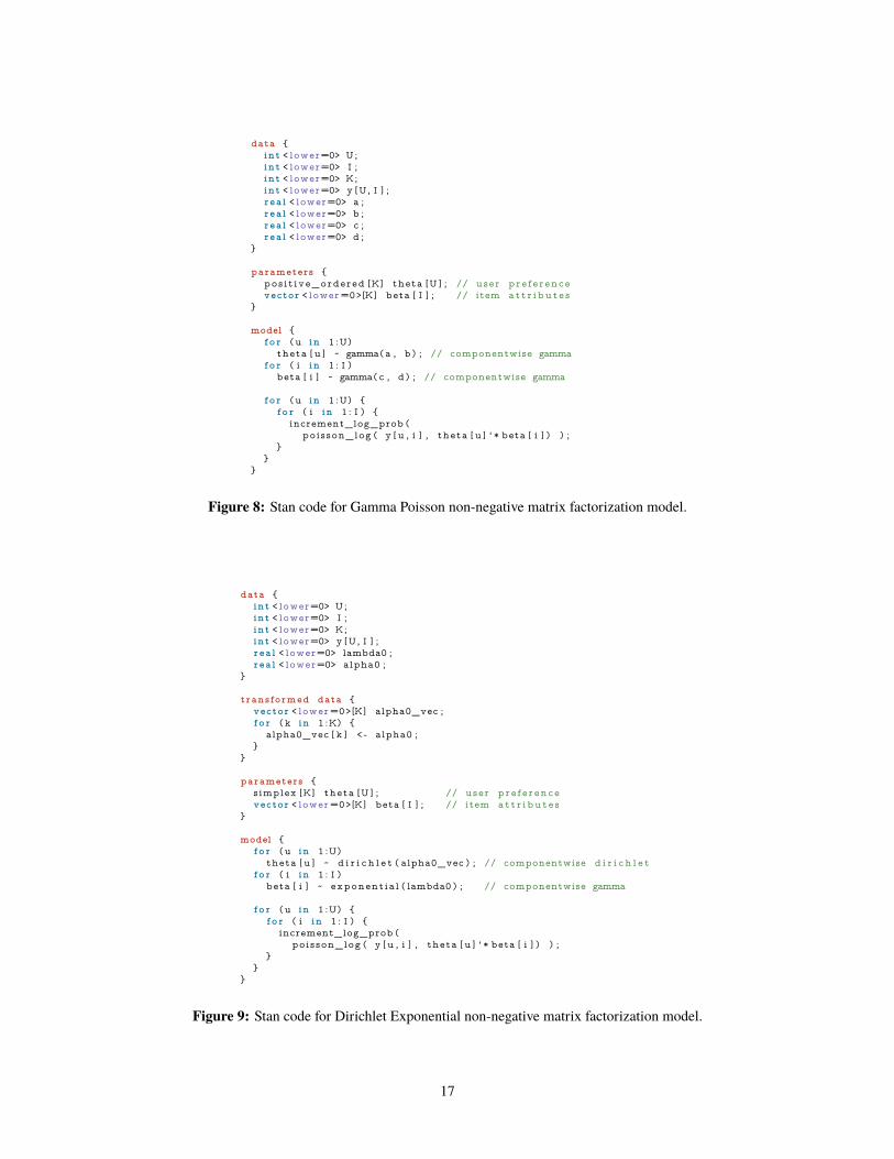
3.2 Exploring nonconjugate Models: Non-negative Matrix Factorization
We continue by exploring two nonconjugate non-negative matrix factorization models: a constrainedGamma Poisson model [24] and a Dirichlet Exponential model. Here, we show how easy it is toexplore new models using ����. In both models, we use the Frey Face dataset, which contains 1956
frames (28 ⇥ 20 pixels) of facial expressions extracted from a video sequence.7���� is an adaptive extension of ���. It is the default sampler in Stan.
7

10
110
210
310
4
�11
�9
�7
�5
Seconds
Aver
age
Log
Pred
ictiv
eADVINUTS
(a) Gamma Poisson Predictive Likelihood
10
110
210
310
4
�600
�400
�200
0
Seconds
Aver
age
Log
Pred
ictiv
e
ADVINUTS
(b) Dirichlet Exponential Predictive Likelihood
(c) Gamma Poisson Factors (d) Dirichlet Exponential Factors
Figure 5: Non-negative matrix factorization of the Frey Faces dataset.
Constrained Gamma Poisson. This is a Gamma Poisson factorization model with an orderingconstraint: each row of the Gamma matrix goes from small to large values. (Details in Appendix H.)
Dirichlet Exponential. This is a nonconjugate Dirichlet Exponential factorization model with aPoisson likelihood. (Details in Appendix I.)
Results. Figure 5 shows average log predictive accuracy as well as ten factors recovered from bothmodels. ���� provides an order of magnitude speed improvement over ���� (Figure 5a). ����struggles with the Dirichlet Exponential model (Figure 5b). In both cases, ��� does not produceany useful samples within a budget of one hour; we omit ��� from the plots.
The Gamma Poisson model (Figure 5c) appears to pick significant frames out of the dataset. TheDirichlet Exponential factors (Figure 5d) are sparse and indicate components of the face that move,such as eyebrows, cheeks, and the mouth.
3.3 Scaling to Large Datasets: Gaussian Mixture Model
We conclude with the Gaussian mixture model (���) example we highlighted earlier. This is anonconjugate ��� applied to color image histograms. We place a Dirichlet prior on the mixtureproportions, a Gaussian prior on the component means, and a lognormal prior on the standard devi-ations. (Details in Appendix J.) We explore the image���� dataset, which has 250 000 images [25].We withhold 10 000 images for evaluation.
In Figure 1a we randomly select 1000 images and train a model with 10 mixture components. ����struggles to find an adequate solution and ��� fails altogether. This is likely due to label switching,which can a�ect ���-based techniques in mixture models [4].
Figure 1b shows ���� results on the full dataset. Here we use ���� with stochastic subsamplingof minibatches from the dataset [3]. We increase the number of mixture components to 30. With aminibatch size of 500 or larger, ���� reaches high predictive accuracy. Smaller minibatch sizes leadto suboptimal solutions, an e�ect also observed in [3]. ���� converges in about two hours.
4 Conclusion
We develop automatic di�erentiation variational inference (����) in Stan. ���� leverages automatictransformations, an implicit non-Gaussian variational approximation, and automatic di�erentiation.
8

This is a valuable tool. We can explore many models, and analyze large datasets with ease. Weemphasize that ���� is currently available as part of Stan; it is ready for anyone to use.
Acknowledgments
We acknowledge our amazing colleagues and funding sources here.
9

References[1] Michael I Jordan, Zoubin Ghahramani, Tommi S Jaakkola, and Lawrence K Saul. An introduc-
tion to variational methods for graphical models. Machine Learning, 37(2):183–233, 1999.
[2] Martin J Wainwright and Michael I Jordan. Graphical models, exponential families, and vari-ational inference. Foundations and Trends in Machine Learning, 1(1-2):1–305, 2008.
[3] Matthew D Ho�man, David M Blei, Chong Wang, and John Paisley. Stochastic variationalinference. The Journal of Machine Learning Research, 14(1):1303–1347, 2013.
[4] Stan Development Team. Stan Modeling Language Users Guide and Reference Manual, 2015.
[5] Matthew D Ho�man and Andrew Gelman. The No-U-Turn sampler. The Journal of MachineLearning Research, 15(1):1593–1623, 2014.
[6] Diederik Kingma and Max Welling. Auto-encoding variational Bayes. arXiv:1312.6114, 2013.
[7] Danilo J Rezende, Shakir Mohamed, and Daan Wierstra. Stochastic backpropagation and ap-proximate inference in deep generative models. In ICML, pages 1278–1286, 2014.
[8] Rajesh Ranganath, Sean Gerrish, and David Blei. Black box variational inference. In AISTATS,pages 814–822, 2014.
[9] Tim Salimans and David Knowles. On using control variates with stochastic approximation forvariational Bayes. arXiv preprint arXiv:1401.1022, 2014.
[10] Michalis Titsias and Miguel Lázaro-Gredilla. Doubly stochastic variational Bayes for non-conjugate inference. In ICML, pages 1971–1979, 2014.
[11] David Wingate and Theophane Weber. Automated variational inference in probabilistic pro-gramming. arXiv preprint arXiv:1301.1299, 2013.
[12] Noah D Goodman, Vikash K Mansinghka, Daniel Roy, Keith Bonawitz, and Joshua B Tenen-baum. Church: A language for generative models. In UAI, pages 220–229, 2008.
[13] Vikash Mansinghka, Daniel Selsam, and Yura Perov. Venture: a higher-order probabilisticprogramming platform with programmable inference. arXiv:1404.0099, 2014.
[14] Frank Wood, Jan Willem van de Meent, and Vikash Mansinghka. A new approach to proba-bilistic programming inference. In AISTATS, pages 2–46, 2014.
[15] John M Winn and Christopher M Bishop. Variational message passing. In Journal of MachineLearning Research, pages 661–694, 2005.
[16] Christopher M Bishop. Pattern Recognition and Machine Learning. Springer New York, 2006.
[17] David J Olive. Statistical Theory and Inference. Springer, 2014.
[18] Manfred Opper and Cédric Archambeau. The variational Gaussian approximation revisited.Neural computation, 21(3):786–792, 2009.
[19] Wolfgang Härdle and Léopold Simar. Applied multivariate statistical analysis. Springer, 2012.
[20] Christian P Robert and George Casella. Monte Carlo statistical methods. Springer, 1999.
[21] John Duchi, Elad Hazan, and Yoram Singer. Adaptive subgradient methods for online learningand stochastic optimization. The Journal of Machine Learning Research, 12:2121–2159, 2011.
[22] Mark Girolami and Ben Calderhead. Riemann manifold langevin and hamiltonian monte carlomethods. Journal of the Royal Statistical Society: Series B, 73(2):123–214, 2011.
[23] Andrew Gelman and Jennifer Hill. Data analysis using regression and multilevel/hierarchicalmodels. Cambridge University Press, 2006.
[24] John Canny. GaP: a factor model for discrete data. In ACM SIGIR, pages 122–129. ACM, 2004.
[25] Mauricio Villegas, Roberto Paredes, and Bart Thomee. Overview of the ImageCLEF 2013Scalable Concept Image Annotation Subtask. In CLEF Evaluation Labs and Workshop, 2013.
10
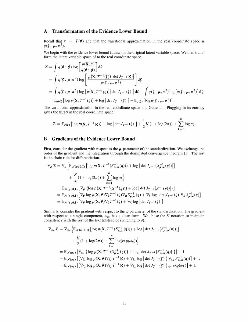
A Transformation of the Evidence Lower Bound
Recall that ⇣ D T .✓/ and that the variational approximation in the real coordinate space isq.⇣ I �; �
2/.
We begin with the evidence lower bound (����) in the original latent variable space. We then trans-form the latent variable space of to the real coordinate space.
L DZ
q.✓ I �/ log
p.X; ✓/
q.✓ I �/
�
d✓
DZ
q.⇣ I �; �
2/ log
"
p
�
X; T
�1.⇣/
�
ˇ
ˇ det JT �1.⇣/
ˇ
ˇ
q.⇣ I �; �
2/
#
d⇣
DZ
q.⇣ I �; �
2/ log
⇥
p
�
X; T
�1.⇣/
�
ˇ
ˇ det JT �1.⇣/
ˇ
ˇ
⇤
d⇣ �Z
q.⇣ I �; �
2/ log
⇥
q.⇣ I �; �
2/
⇤
d⇣
D Eq.⇣/
⇥
log p
�
X; T
�1.⇣/
�
C logˇ
ˇ det JT �1.⇣/
ˇ
ˇ
⇤
� Eq.⇣/
⇥
log q.⇣ I �; �
2/
⇤
The variational approximation in the real coordinate space is a Gaussian. Plugging in its entropygives the ���� in the real coordinate space
L D Eq.⇣/
⇥
log p
�
X; T
�1.⇣/
�
C logˇ
ˇ det JT �1.⇣/
ˇ
ˇ
⇤
C 1
2
K .1C log.2⇡//CK
X
kD1
log �k :
B Gradients of the Evidence Lower Bound
First, consider the gradient with respect to the � parameter of the standardization. We exchange theorder of the gradient and the integration through the dominated convergence theorem [1]. The restis the chain rule for di�erentiation.
r�L D r�
n
EN .⌘ I 0;I/
⇥
log p
�
X; T
�1.S
�1�;!.⌘//
�
C logˇ
ˇ det JT �1
�
S
�1�;!.⌘/
�
ˇ
ˇ
⇤
C K
2
.1C log.2⇡//CK
X
kD1
log �k
o
D EN .⌘ I 0;I/
⇥
r�
˚
log p
�
X; T
�1.S
�1.⌘//
�
C logˇ
ˇ det JT �1
�
S
�1.⌘/
�
ˇ
ˇ
⇤
D EN .⌘ I 0;I/
⇥
r✓ log p.X; ✓/r⇣T
�1.⇣/r�S
�1�;!.⌘/Cr⇣ log
ˇ
ˇ det JT �1.⇣/
ˇ
ˇr�S
�1�;!.⌘/
⇤
D EN .⌘ I 0;I/
⇥
r✓ log p.X; ✓/r⇣T
�1.⇣/Cr⇣ log
ˇ
ˇ det JT �1.⇣/
ˇ
ˇ
⇤
Similarly, consider the gradient with respect to the ! parameter of the standardization. The gradientwith respect to a single component, !k , has a clean form. We abuse the r notation to maintainconsistency with the rest of the text (instead of switching to @).
r!kL D r!k
n
EN .⌘ I 0;I/
⇥
log p
�
X; T
�1.S
�1�;!.⌘//
�
C logˇ
ˇ det JT �1
�
S
�1�;!.⌘/
�
ˇ
ˇ
⇤
C K
2
.1C log.2⇡//CK
X
kD1
log.exp.!k//
o
D EN .⌘k/
⇥
r!k
˚
log p
�
X; T
�1.S
�1�;!.⌘//
�
C logˇ
ˇ det JT �1
�
S
�1�;!.⌘/
�
ˇ
ˇ
⇤
C 1
D EN .⌘k/
⇥�
r✓klog p.X; ✓/r⇣k
T
�1.⇣/Cr⇣k
logˇ
ˇ det JT �1.⇣/
ˇ
ˇ
�
r!kS
�1�;!.⌘//
⇤
C 1:
D EN .⌘k/
⇥�
r✓klog p.X; ✓/r⇣k
T
�1.⇣/Cr⇣k
logˇ
ˇ det JT �1.⇣/
ˇ
ˇ
�
⌘k exp.!k/
⇤
C 1:
11

C Running ���� in Stan
Use git to checkout the feature/bbvb branch from https://github.com/stan-dev/stan. Fol-low instructions to build Stan. Then download cmdStan from https://github.com/stan-
dev/cmdstan. Follow instructions to build cmdStan and compile your model. You are then readyto run ����.The syntax is
./myModel experimental variational
grad_samples=M ( M D 1 default )
data file=myData.data.R
output file=output_advi.csv
diagnostic_file=elbo_advi.csv
where myData.data.R is the dataset in the R language dump format. output_advi.csv containssamples from the posterior and elbo_advi.csv reports the ����.
D Transformations of Continuous Probability Densities
We present a brief summary of transformations, largely based on [2].
Consider a univariate (scalar) random variable X with probability density function fX .x/. Let X Dsupp.fX .x// be the support of X . Now consider another random variable Y defined as Y D T .X/.Let Y D supp.fY .y// be the support of Y .
If T is a one-to-one and di�erentiable function from X to Y, then Y has probability density function
fY .y/ D fX
�
T
�1.y/
�
ˇ
ˇ
ˇ
ˇ
dT
�1.y/
dy
ˇ
ˇ
ˇ
ˇ
:
Let us sketch a proof. Consider the cumulative density function Y . If the transformation T is in-creasing, we directly apply its inverse to the cdf of Y . If the transformation T is decreasing, weapply its inverse to one minus the cdf of Y . The probability density function is the derivative of thecumulative density function. These things combined give the absolute value of the derivative above.
The extension to multivariate variables X and Y requires a multivariate version of the absolute valueof the derivative of the inverse transformation. This is the the absolute determinant of the Jacobian,j det JT �1.Y /j where the Jacobian is
JT �1.Y / D
˙@T �1
1
@y1� � � @T �1
1
@yK
:
:
:
:
:
:
@T �1K
@y1� � � @T �1
K
@yK
⌥:
Intuitively, the Jacobian describes how a transformation warps unit volumes across spaces. Thismatters for transformations of random variables, since probability density functions must alwaysintegrate to one. If the transformation is linear, then we can drop the Jacobian adjustment; it evaluatesto one. Similarly, a�ne transformations, like elliptical standardizations, do not require Jacobianadjustments; they preserve unit volumes.
E Setting a Stepsize Sequence for ����
We use adaGrad [3] to adaptively set the stepsize sequence in ����. While adaGrad o�ers attractiveconvergence properties, in practice it can be slow because it has infinite memory. (It tracks the normof the gradient starting from the beginning of the optimization.) In ���� we randomly initialize thevariational approximation, which can be far from the true posterior. This makes adaGrad take verysmall steps for the rest of the optimization, thus slowing convergence. Limiting adaGrad’s memoryspeeds up convergence in practice, an e�ect also observed in training neural networks [4]. (See [5]for an analysis of these trade-o�s and a method that combines benefits from both.)
12

Consider the stepsize ⇢
.i/ and a gradient vector g
.i/ at iteration i . The kth element of ⇢
.i/ is⇢
.i/k D
⌘
⌧ Cq
s
.i/k
where, in adaGrad, s is the gradient vector squared, summed over all times steps since the start ofthe optimization. Instead, we limit this to the past ten iterations and compute s as
s
.i/k D g
2k
.i�10/ C g
2k
.i�9/ C � � �C g
2k
.i/:
(In practice, we implement this recursively to save memory.) We set ⌘ D 0:1 and ⌧ D 1 as the defaultvalues we use in Stan.
F Linear Regression with Automatic Relevance Determination
Linear regression with automatic relevance determination (���) is a high-dimensional sparse re-gression model [6, 7]. We describe the model below. Stan code is in Figure 6.
The inputs are X D x1WN where each xn is D-dimensional. The outputs are y D y1WN where eachyn is 1-dimensional. The weights vector w is D-dimensional. The likelihood
p.y j X; w; ⌧/ DNY
nD1
N�
yn j w>xn ; ⌧
�1�
describes measurements corrupted by iid Gaussian noise with unknown variance ⌧
�1.
The ��� prior and hyper-prior structure is as followsp.w; ⌧; ˛/ D p.w; ⌧ j ˛/p.˛/
D N�
w j 0 ; .⌧diagŒ˛ç/
�1�
Gam.⌧ j a0; b0/
DY
iD1
Gam.˛i j c0; d0/
where ˛ is a D-dimensional hyper-prior on the weights, where each component gets its own inde-pendent Gamma prior.
We simulate data such that only half the regressions have predictive power. The results in Figure 4ause a0 D b0 D c0 D d0 D 1 as hyper-parameters for the Gamma priors.
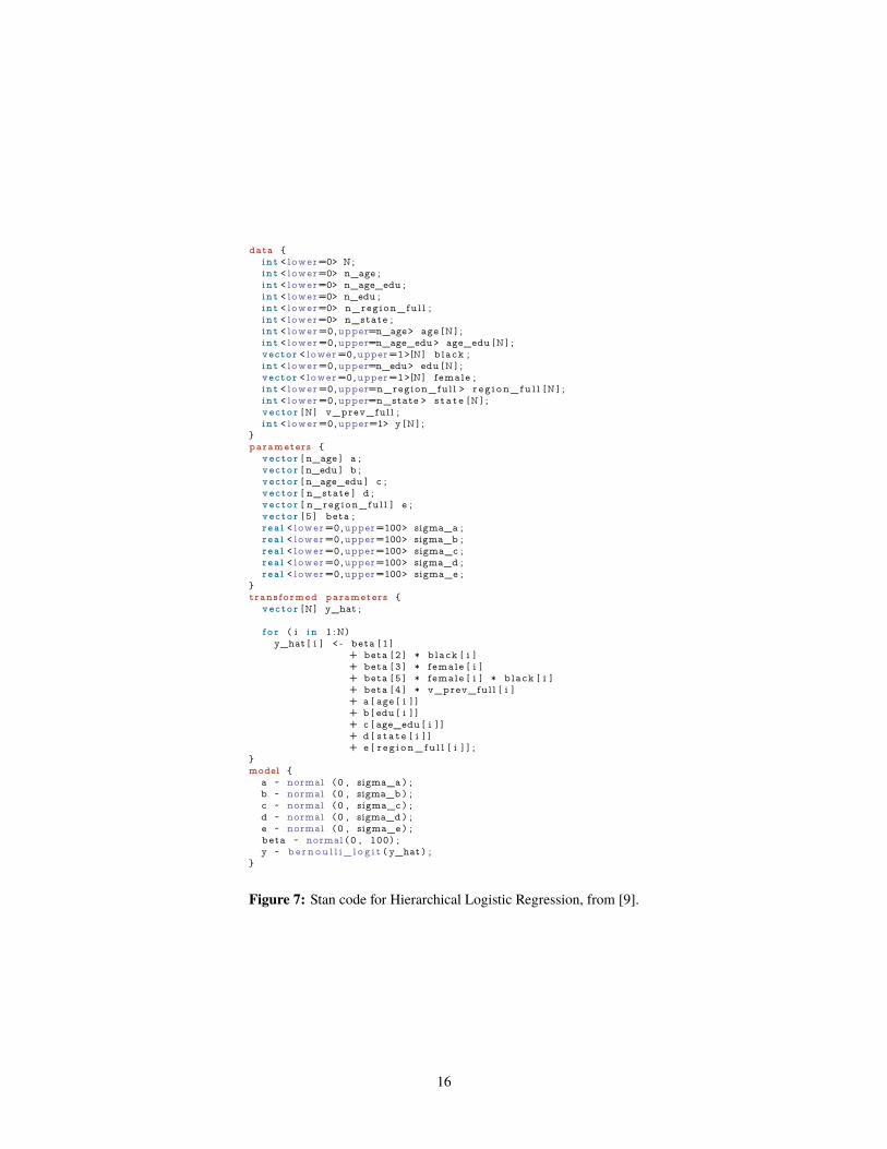
G Hierarchical Logistic Regression
Hierarchical logistic regression models dependencies in an intuitive and powerful way. We study amodel of voting preferences from the 1988 United States presidential election. Chapter 14.1 of [8]motivates the model and explains the dataset. We also describe the model below. Stan code is inFigure 7, based on [9].
Pr.yn D 1/ D �
✓
ˇ
0 C ˇ
female � femalen C ˇ
black � blackn C ˇ
female.black � female.blackn
C ˛
agekŒnç C ˛
edulŒnç C ˛
age.edukŒnç;lŒnç C ˛
statej Œnç
◆
˛
statej ⇠ N
⇣
˛
regionmŒj ç C ˇ
v.prev � v.prevj ; �
2state
⌘
where �.�/ is the sigmoid function (also know as the logistic function).
The hierarchical variables are˛
agek ⇠ N
⇣
0 ; �
2age
⌘
for k D 1; : : : ; K
˛
edul ⇠ N
�
0 ; �
2edu
�
for l D 1; : : : ; L
˛
age.eduk;l ⇠ N
⇣
0 ; �
2age.edu
⌘
for k D 1; : : : ; K; l D 1; : : : ; L
˛
regionm ⇠ N
⇣
0 ; �
2region
⌘
for m D 1; : : : ; M:
The variance terms all have uniform hyper-priors, constrained between 0 and 100.
13

H Non-negative Matrix Factorization: Constrained Gamma Poisson Model
The Gamma Poisson factorization model is a powerful way to analyze discrete data matrices [10, 11].
Consider a U ⇥ I matrix of observations. We find it helpful to think of u D f1; � � � ; U g as usersand i D f1; � � � ; I g as items, as in a recommendation system setting. The generative process for aGamma Poisson model with K factors is
1. For each user u in f1; � � � ; U g:✏ For each component k, draw ✓uk ⇠ Gam.a0; b0/.
2. For each item i in f1; � � � ; I g:✏ For each component k, draw ˇik ⇠ Gam.c0; d0/.
3. For each user and item:✏ Draw the observation yui ⇠ Poisson.✓
>u ˇi /.
A potential downfall of this model is that it is not uniquely identifiable: scaling ✓u by ˛ and ˇi by ˛
�1
gives the same likelihood. One way to contend with this is to constrain either vector to be a positive,ordered vector during inference. We constrain each ✓u vector in our model in this fashion. Stan codeis in Figure 8. We set K D 10 and all the Gamma hyper-parameters to 1 in our experiments.
I Non-negative Matrix Factorization: Dirichlet Exponential Model
Another model for discrete data is a Dirichlet Exponential model. The Dirichlet enforces uniquenesswhile the exponential promotes sparsity. This is a non-conjugate model that does not appear to havebeen studied in the literature.
The generative process for a Dirichlet Exponential model with K factors is
1. For each user u in f1; � � � ; U g:✏ Draw the K-vector ✓u ⇠ Dir.˛0/.
2. For each item i in f1; � � � ; I g:✏ For each component k, draw ˇik ⇠ Exponential.�0/.
3. For each user and item:✏ Draw the observation yui ⇠ Poisson.✓
>u ˇi /.
Stan code is in Figure 9. We set K D 10, ˛0 D 1000 for each component, and �0 D 0:1. With thisconfiguration of hyper-parameters, the factors ˇi are sparse and appear interpretable.
J Gaussian Mixture Model
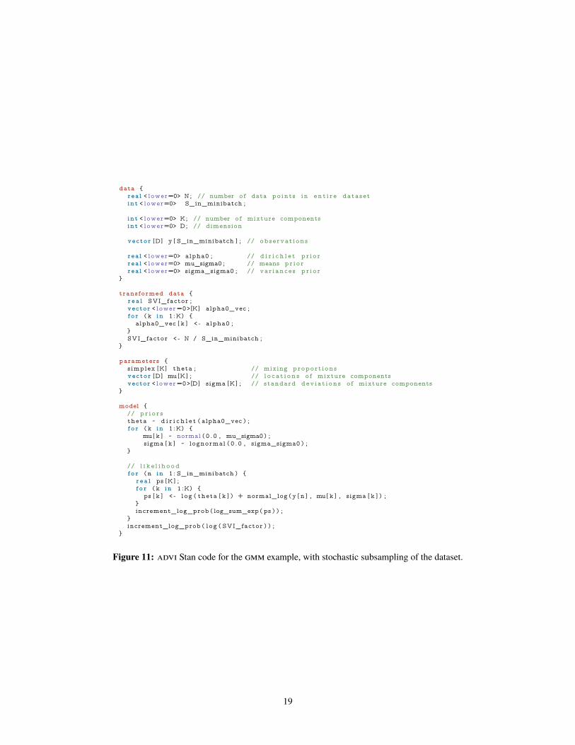
The Gaussian mixture model (���) is a powerful probability model. We use it to group a dataset ofnatural images based on their color histograms. We build a high-dimensional ��� with a Gaussianprior for the mixture means, a lognormal prior for the mixture standard deviations, and a Dirichletprior for the mixture components.
The images are in X D x1WN where each xn is D-dimensional and there are N observations. Thelikelihood for the images is
p.X j ✓; �; � / DNY
nD1
KY
kD1
✓k
DY
dD1
N .xnd j �kd ; �kd /
with a Dirichlet prior for the mixture proportions
p.✓/ D Dir.✓ I ˛0/;
14

a Gaussian prior for the mixture means
p.�/ DD
Y
kD1
DY
dD1
N .�kd I 0; ��/
and a lognormal prior for the mixture standard deviations
p.� / DD
Y
kD1
DY
dD1
logNormal.�kd I 0; �� /
The dimension of the color histograms in the image���� dataset is D D 576. These a concatenationof three 192-length histograms, one for each color channel (red, green, blue) of the images.
We scale the image histograms to have zero mean and unit variance and set ˛0 D 10 000, �� D0:1 and ��. ���� code is in Figure 10. The stochastic data subsampling version of the code is inFigure 11.
data {
int < lower=0> N; // number o f data items
int < lower=0> D; // dimension o f input f e a t u r e s
matrix [N,D] x ; // input matrix
vecto r [N] y ; // output vec to r
// hyperparameters f o r Gamma p r i o r s
r ea l < lower=0> a0 ;
r ea l < lower=0> b0 ;
r ea l < lower=0> c0 ;
r ea l < lower=0> d0 ;
}
parameters {
vecto r [D] w; // weights ( c o e f f i c i e n t s ) vec to r
r e a l < lower=0> sigma2 ; // va r i ance
vector < lower =0>[D] alpha ; // hyper - parameters on weights
}
trans formed parameters {
r e a l sigma ; // standard d e v i a t i o n
vecto r [D] one_over_sqrt_alpha ; // numer ica l s t a b i l i t y
sigma < - s q r t ( sigma2 ) ;
f o r ( i in 1 :D) {
one_over_sqrt_alpha [ i ] < - 1 / s q r t ( alpha [ i ] ) ;
}
}
model {
// alpha : hyper - p r i o r on weights
alpha ~ gamma( c0 , d0 ) ;
// sigma2 : p r i o r on var i ance
sigma2 ~ inv_gamma( a0 , b0 ) ;
// w: p r i o r on weights
w ~ normal (0 , sigma * one_over_sqrt_alpha ) ;
// y : l i k e l i h o o d
y ~ normal ( x * w, sigma ) ;
}
Figure 6: Stan code for Linear Regression with Automatic Relevance Determination.
15
data {
int < lower=0> N;
int < lower=0> n_age ;
int < lower=0> n_age_edu ;
int < lower=0> n_edu ;
int < lower=0> n_reg ion_fu l l ;
int < lower=0> n_state ;
int < lower =0,upper=n_age> age [N ] ;
int < lower =0,upper=n_age_edu> age_edu [N ] ;
vector < lower =0,upper =1>[N] b lack ;
int < lower =0,upper=n_edu> edu [N ] ;
vector < lower =0,upper =1>[N] female ;
int < lower =0,upper=n_region_ful l > r e g i o n _ f u l l [N ] ;
int < lower =0,upper=n_state > s t a t e [N ] ;
vec to r [N] v_prev_ful l ;
int < lower =0,upper=1> y [N ] ;
}
parameters {
vec to r [ n_age ] a ;
vec to r [ n_edu ] b ;
vec to r [ n_age_edu ] c ;
vec to r [ n_state ] d ;
vec to r [ n_reg ion_fu l l ] e ;
vec to r [ 5 ] beta ;
r ea l < lower =0,upper=100> sigma_a ;
r ea l < lower =0,upper=100> sigma_b ;
r ea l < lower =0,upper=100> sigma_c ;
r ea l < lower =0,upper=100> sigma_d ;
r ea l < lower =0,upper=100> sigma_e ;
}
trans formed parameters {
vec to r [N] y_hat ;
f o r ( i in 1 :N)
y_hat [ i ] < - beta [ 1 ]
+ beta [ 2 ] * b lack [ i ]
+ beta [ 3 ] * female [ i ]
+ beta [ 5 ] * female [ i ] * b lack [ i ]
+ beta [ 4 ] * v_prev_ful l [ i ]
+ a [ age [ i ] ]
+ b [ edu [ i ] ]
+ c [ age_edu [ i ] ]
+ d [ s t a t e [ i ] ]
+ e [ r e g i o n _ f u l l [ i ] ] ;
}
model {
a ~ normal (0 , sigma_a ) ;
b ~ normal (0 , sigma_b ) ;
c ~ normal (0 , sigma_c ) ;
d ~ normal (0 , sigma_d ) ;
e ~ normal (0 , sigma_e ) ;
beta ~ normal (0 , 100) ;
y ~ b e r n o u l l i _ l o g i t ( y_hat ) ;
}
Figure 7: Stan code for Hierarchical Logistic Regression, from [9].
16
data {
int < lower=0> U;
int < lower=0> I ;
int < lower=0> K;
int < lower=0> y [U, I ] ;
r ea l < lower=0> a ;
r ea l < lower=0> b ;
r ea l < lower=0> c ;
r ea l < lower=0> d ;
}
parameters {
pos i t i v e_orde r ed [K] theta [U ] ; // user p r e f e r e n c e
vector < lower =0>[K] beta [ I ] ; // item a t t r i b u t e s
}
model {
f o r (u in 1 :U)
theta [ u ] ~ gamma( a , b) ; // componentwise gamma
f o r ( i in 1 : I )
beta [ i ] ~ gamma( c , d) ; // componentwise gamma
f o r (u in 1 :U) {
f o r ( i in 1 : I ) {
increment_log_prob (
po is son_log ( y [ u , i ] , theta [ u ] ‘ * beta [ i ] ) ) ;
}
}
}
Figure 8: Stan code for Gamma Poisson non-negative matrix factorization model.
data {
int < lower=0> U;
int < lower=0> I ;
int < lower=0> K;
int < lower=0> y [U, I ] ;
r ea l < lower=0> lambda0 ;
r ea l < lower=0> alpha0 ;
}
trans formed data {
vector < lower =0>[K] alpha0_vec ;
f o r ( k in 1 :K) {
alpha0_vec [ k ] < - alpha0 ;
}
}
parameters {
s implex [K] theta [U ] ; // user p r e f e r e n c e
vector < lower =0>[K] beta [ I ] ; // item a t t r i b u t e s
}
model {
f o r (u in 1 :U)
theta [ u ] ~ d i r i c h l e t ( alpha0_vec ) ; // componentwise d i r i c h l e t
f o r ( i in 1 : I )
beta [ i ] ~ exponent i a l ( lambda0 ) ; // componentwise gamma
f o r (u in 1 :U) {
f o r ( i in 1 : I ) {
increment_log_prob (
po is son_log ( y [ u , i ] , theta [ u ] ‘ * beta [ i ] ) ) ;
}
}
}
Figure 9: Stan code for Dirichlet Exponential non-negative matrix factorization model.
17

data {
int < lower=0> N; // number o f data po in t s in e n t i r e da ta s e t
int < lower=0> K; // number o f mixture components
int < lower=0> D; // dimension
vec to r [D] y [N ] ; // o b s e r v a t i o n s
r ea l < lower=0> alpha0 ; // d i r i c h l e t p r i o r
r ea l < lower=0> mu_sigma0 ; // means p r i o r
r ea l < lower=0> sigma_sigma0 ; // v a r i a n c e s p r i o r
}
trans formed data {
vector < lower =0>[K] alpha0_vec ;
f o r ( k in 1 :K) {
alpha0_vec [ k ] < - alpha0 ;
}
}
parameters {
s implex [K] theta ; // mixing pr op o r t i o n s
vec to r [D] mu[K ] ; // l o c a t i o n s o f mixture components
vector < lower =0>[D] sigma [K ] ; // standard d e v i a t i o n s o f mixture components
}
model {
// p r i o r s
theta ~ d i r i c h l e t ( alpha0_vec ) ;
f o r ( k in 1 :K) {
mu[ k ] ~ normal ( 0 . 0 , mu_sigma0 ) ;
sigma [ k ] ~ lognormal ( 0 . 0 , sigma_sigma0 ) ;
}
// l i k e l i h o o d
f o r (n in 1 :N) {
r e a l ps [K ] ;
f o r ( k in 1 :K) {
ps [ k ] < - l og ( theta [ k ] ) + normal_log ( y [ n ] , mu[ k ] , sigma [ k ] ) ;
}
increment_log_prob ( log_sum_exp ( ps ) ) ;
}
}
Figure 10: ���� Stan code for the ��� example.
18
data {
r ea l < lower=0> N; // number o f data po in t s in e n t i r e da ta s e t
int < lower=0> S_in_minibatch ;
int < lower=0> K; // number o f mixture components
int < lower=0> D; // dimension
vec to r [D] y [ S_in_minibatch ] ; // o b s e r v a t i o n s
r ea l < lower=0> alpha0 ; // d i r i c h l e t p r i o r
r ea l < lower=0> mu_sigma0 ; // means p r i o r
r ea l < lower=0> sigma_sigma0 ; // v a r i a n c e s p r i o r
}
trans formed data {
r e a l SVI_factor ;
vector < lower =0>[K] alpha0_vec ;
f o r ( k in 1 :K) {
alpha0_vec [ k ] < - alpha0 ;
}
SVI_factor < - N / S_in_minibatch ;
}
parameters {
s implex [K] theta ; // mixing pr op o r t i o n s
vec to r [D] mu[K ] ; // l o c a t i o n s o f mixture components
vector < lower =0>[D] sigma [K ] ; // standard d e v i a t i o n s o f mixture components
}
model {
// p r i o r s
theta ~ d i r i c h l e t ( alpha0_vec ) ;
f o r ( k in 1 :K) {
mu[ k ] ~ normal ( 0 . 0 , mu_sigma0 ) ;
sigma [ k ] ~ lognormal ( 0 . 0 , sigma_sigma0 ) ;
}
// l i k e l i h o o d
f o r (n in 1 : S_in_minibatch ) {
r e a l ps [K ] ;
f o r ( k in 1 :K) {
ps [ k ] < - l og ( theta [ k ] ) + normal_log ( y [ n ] , mu[ k ] , sigma [ k ] ) ;
}
increment_log_prob ( log_sum_exp ( ps ) ) ;
}
increment_log_prob ( l og ( SVI_factor ) ) ;
}
Figure 11: ���� Stan code for the ��� example, with stochastic subsampling of the dataset.
19

References[1] Erhan Çınlar. Probability and Stochastics. Springer, 2011.
[2] David J Olive. Statistical Theory and Inference. Springer, 2014.
[3] John Duchi, Elad Hazan, and Yoram Singer. Adaptive subgradient methods for online learningand stochastic optimization. The Journal of Machine Learning Research, 12:2121–2159, 2011.
[4] T Tieleman and G Hinton. Lecture 6.5-rmsprop: Divide the gradient by a running average ofits recent magnitude. COURSERA: Neural Networks for Machine Learning, 4, 2012.
[5] Diederik Kingma and Jimmy Ba. Adam: A method for stochastic optimization. arXiv preprintarXiv:1412.6980, 2014.
[6] Christopher M Bishop. Pattern Recognition and Machine Learning. Springer New York, 2006.
[7] Jan Drugowitsch. Variational Bayesian inference for linear and logistic regression. arXivpreprint arXiv:1310.5438, 2013.
[8] Andrew Gelman and Jennifer Hill. Data analysis using regression and multilevel/hierarchicalmodels. Cambridge University Press, 2006.
[9] Stan Development Team. Stan Modeling Language Users Guide and Reference Manual, 2015.
[10] John Canny. GaP: a factor model for discrete data. In ACM SIGIR, pages 122–129. ACM, 2004.
[11] Ali Taylan Cemgil. Bayesian inference for nonnegative matrix factorisation models. Computa-tional Intelligence and Neuroscience, 2009, 2009.
20