automotive science and mathematics · 2.3 making sense of data 17 discrete variables 17 continuous...
TRANSCRIPT


Automotive Science and Mathematics

This page intentionally left blank
Automotive Science andMathematics
Allan Bonnick
AMSTERDAM • BOSTON • HEIDELBERG • LONDON • NEW YORK • OXFORDPARIS • SAN DIEGO • SAN FRANCISCO • SINGAPORE • SYDNEY • TOKYO
Butterworth-Heinemann is an imprint of Elsevier

Butterworth-Heinemann is an imprint of ElsevierLinacre House, Jordan Hill, Oxford OX2 8DP, UK30 Corporate Drive, Suite 400, Burlington, MA 01803, USA
First edition 2008
Copyright © 2008, Allan Bonnick. Published by Elsevier Ltd. All rights reserved
The right of Allan Bonnick to be identified as the author of this work has beenasserted in accordance with the Copyright, Designs and Patents Act 1988
No part of this publication may be reproduced, stored in a retrieval systemor transmitted in any form or by any means electronic, mechanical, photocopying,recording or otherwise without the prior written permission of the publisher
Permissions may be sought directly from Elsevier’s Science & Technology RightsDepartment in Oxford, UK: phone (+44) (0) 1865 843830; fax (+44) (0) 1865 853333;email: [email protected]. Alternatively you can submit your request online byvisiting the Elsevier web site at http://elsevier.com/locate/permissions, and selectingObtaining permission to use Elsevier material
NoticeNo responsibility is assumed by the publisher for any injury and/or damage to personsor property as a matter of products liability, negligence or otherwise, or from any useor operation of any methods, products, instructions or ideas contained in the materialherein. Because of rapid advances in the medical sciences, in particular, independentverification of diagnoses and drug dosages should be made
British Library Cataloguing in Publication DataA catalogue record for this book is available from the British Library
Library of Congress Cataloging-in-Publication DataA catalog record for this book is available from the Library of Congress
ISBN: 978-0-7506-8522-1
For information on all Butterworth-Heinemann publicationsvisit our web site at books.elsevier.com
Printed and bound in Hungary
08 09 10 10 9 8 7 6 5 4 3 2 1
Working together to grow libraries in developing countries
www.elsevier.com | www.bookaid.org | www.sabre.org

Contents
Preface xvii
Units and symbols xviii
Glossary xix
1 Arithmetic 11.1 Terminology of number systems 11.2 The decimal system 1
Addition and subtraction of decimals 2Multiplication and division – decimals 2
1.3 Degrees of accuracy 4Rounding numbers 4
1.4 Accuracy in calculation 41.5 Powers and roots and standard form 4
General rules for indices 51.6 Standard form 5
Multiplying and dividing numbers in standard form 51.7 Factors 61.8 Fractions 6
Addition and subtraction 6Fractions and whole numbers 6Combined addition and subtraction 7Multiplication and division of fractions 7Order of performing operations in problems involving fractions 7
1.9 Ratio and proportion. Percentages 8Examples of ratios in vehicle technology 8
1.10 The binary system 10Most significant bit (MSB) 10Hexadecimal 10Converting base 10 numbers to binary 10Uses of binary numbers in vehicle systems 10
1.11 Directed numbers 11Rules for dealing with directed numbers 11
1.12 Summary of main points 121.13 Exercises 12

vi Contents
2 Statistics – An introduction 162.1 Definition 162.2 Collecting and sorting raw data 172.3 Making sense of data 17
Discrete variables 17Continuous variables 17
2.4 Descriptive statistics – pictographs 18Pie charts 18
2.5 Interpreting data. Statistical inference 19Frequency and tally charts 19The tally chart and frequency distribution 19
2.6 Importance of the shape of a frequency distribution 20The histogram 20The frequency polygon 20Cumulative frequency 21
2.7 Interpreting statistics 22Sampling 22
2.8 Features of the population that are looked for in a sample 22Average 22
2.9 The normal distribution 23Importance of the normal distribution 24Other ways of viewing frequency distributions – quartiles, deciles,
percentiles 252.10 Summary of main points 262.11 Exercises 26
3 Algebra and graphs 293.1 Introduction 293.2 Formulae 293.3 Evaluating formulae 293.4 Processes in algebra 30
Brackets 303.5 Algebraic expressions and simplification 30
Expression 303.6 Factorising 313.7 Equations 31
Solving equations 313.8 Transposition of formulae 333.9 Graphs 34
Variables 34Scales 34Coordinates 35
3.10 Graphs and equations 36The straight-line graph 36
3.11 Summary of main points 37

Contents vii
3.12 Exercises 38Exercises – Section 3.3 38Exercises – Section 3.4 38Exercises – Section 3.5 38Exercises – Section 3.6 38Exercises – Section 3.7 38Exercises – Section 3.8 38Exercises – Section 3.10 38
4 Geometry and trigonometry 414.1 Angles 41
Angular measurement 41Angles and rotation 41
4.2 Examples of angles in automotive work 42Angles and lines 43Adding and subtracting angles 43
4.3 Types of angle 44Adjacent angles 44Opposite angles 44Corresponding angles 44Alternate angles 44Supplementary angles 44Complementary angles 44
4.4 Types of triangle 45Acute angled triangle 45Obtuse angled triangle 45Equilateral triangle 45Isosceles triangle 45Scalene triangle 45Right angled triangle 46Labelling sides and angles of a triangle 46Sum of the three angles of a triangle 46
4.5 Pythagoras’ theorem 464.6 Circles 46
Ratio of diameter and circumference � 47Length of arc 47
4.7 Timing marks 474.8 Wheel revolutions and distance travelled 484.9 Valve opening area 484.10 Trigonometry 484.11 Using sines, cosines and tangents 49
Sines 49Cosines 50Tangents 51
4.12 Summary of formulae 52

viii Contents
4.13 Exercises 52Exercises – Section 4.2 53Exercises – Section 4.3 53Exercises – Section 4.4 54Exercises – Section 4.5 55Exercises – Section 4.6 55
5 Forces 585.1 Force 585.2 Types of force – examples 585.3 Describing forces 585.4 Graphical representation of a force 585.5 Addition of forces 595.6 Parallelogram of forces 605.7 Triangle of forces 605.8 Resolution of forces 615.9 Mass 625.10 Equilibrium 625.11 Pressure 625.12 Pressure in hydraulic systems 635.13 Hooke’s law 645.14 Practical applications 655.15 Summary 655.16 Exercises 65
6 Materials – Stress, strain, elasticity 686.1 Introduction 686.2 Stress 68
Types of stress 686.3 Tensile test 696.4 Examples of stress and strain 706.5 Stress raisers 716.6 Strain 72
Shear strain 726.7 Elasticity 73
Stress, strain, elasticity 736.8 Tensile strength 736.9 Factor of safety 746.10 Torsional stress 746.11 Strain energy 756.12 Strength of materials 756.13 Other terms used in describing materials 756.14 Non-ferrous metals 766.15 Non-metallic materials 76
Kevlar 766.16 Recycling of materials 77

Contents ix
6.17 Summary of main formulae 776.18 Exercises 77
7 Levers and moments, torque and gears 797.1 Levers 797.2 Principles of leverage 797.3 The principle of moments 797.4 The bell crank lever 81
A practical application of the bell crank lever 817.5 Axle loadings 827.6 Torque 837.7 Engine torque 837.8 Leverage and gears 84
Torque multiplication 84Drivers and driven 85
7.9 Gear trains: calculating gear ratios 85Spur gear ratios 85
7.10 Couples 857.11 Summary of main points 857.12 Exercises 86
8 Work energy, power and machines 898.1 Work 898.2 Power 898.3 Work done by a torque 908.4 Work done by a constantly varying force 90
Mid-ordinate method for calculating work done 918.5 Energy 92
Potential energy 92Chemical energy 92Conservation of energy 92Energy equation 92Kinetic energy 92Energy of a falling body 93Kinetic energy of rotation 93
8.6 Machines 94Mechanical advantage 94Velocity ratio (movement ratio) 95Efficiency of a machine 95Work done against friction 95A steering mechanism as a machine 95
8.7 Summary of formulae 978.8 Exercises 98

x Contents
9 Friction 999.1 Introduction 99
Coefficient of friction 99Static friction 100Sliding friction 100
9.2 Making use of friction 100Clutch 100Belt drive 101
9.3 Brakes 103Drum brake – basic principle 103Disc brake 103Tyres 105Braking efficiency 106
9.4 Angle of friction 1079.5 Inclined plane 108
Inclined plane without friction 108Inclined plane with friction 108
9.6 Screw thread 108V-thread 109
9.7 Friction in a journal bearing 1109.8 Summary of formulae 1119.9 Exercises 111
10 Velocity and acceleration, speed 11310.1 Speed and velocity 11310.2 Acceleration 11310.3 Velocity–time graph 113
Uniform velocity 113Uniform acceleration 113
10.4 Equations of motion and their application to vehicle technology 11410.5 Force, mass and acceleration 115
Newton’s laws of motion 11510.6 Relation between mass and weight 11510.7 Inertia 11510.8 Motion under gravity 11610.9 Angular (circular) motion 11610.10 Equations of angular motion 11610.11 Relation between angular and linear velocity 11710.12 Centripetal acceleration 117
Accelerating torque 11810.13 Exercises 119
11 Vehicle dynamics 12011.1 Load transfer under acceleration 12011.2 Static reactions 12011.3 Vehicle under acceleration 121

Contents xi
11.4 Vehicle acceleration – effect of load transfer 122Front wheel drive 122Maximum acceleration – rear wheel drive 123Four wheel drive – fixed 123Four wheel drive – with third differential 123
11.5 Accelerating force – tractive effort 12311.6 Tractive resistance 12311.7 Power required to propel vehicle 124
Power available 12411.8 Forces on a vehicle on a gradient – gradient resistance 12611.9 Gradeability 12611.10 Vehicle power on a gradient 12811.11 Vehicle on a curved track 128
Overturning speed 128Skidding speed 130
11.12 Summary of formulae 13011.13 Exercises 130
12 Balancing and vibrations 13212.1 Introduction 13212.2 Balance of rotating masses acting in the same plane (coplanar) 13212.3 Balancing of a number of forces acting in the same plane of revolution
(coplanar forces) 13312.4 Wheel and tyre balance 13412.5 Engine balance 13512.6 Balance in a single-cylinder engine 13512.7 Primary and secondary forces 136
Graph of primary and secondary forces 13612.8 Secondary force balancer 137
Harmonics 13712.9 Balance of rotating parts of the single cylinder engine 13812.10 Four-cylinder in-line engine balance 13912.11 Couples and distance between crank throws 13912.12 Simple harmonic motion (SHM) 13912.13 Applications of SHM 141
Vibration of a helical coil spring 14112.14 Torsional vibration 14212.15 Free vibrations 142
Example of free vibrations 14212.16 Forced vibrations 143
Resonance 143Driveline vibrations 143Damping 143Vibration dampers 143Dual mass flywheel 144Cams 144

xii Contents
12.17 Summary of formulae 14612.18 Exercises 146
13 Heat and temperature 14813.1 Temperature 148
Thermodynamic temperature scale (Kelvin) 148Cooling system temperature 148
13.2 Standard temperature and pressure (STP) 14813.3 Thermal expansion 14813.4 Heat 149
Sensible heat 149Latent heat 149Specific latent heat 149Specific heat capacity 150Quantity of heat 150
13.5 Heat transfer 150Conduction 150Convection 150Radiation 151
13.6 Heating, expansion and compression of gases 151Absolute pressure 151Absolute temperature 151
13.7 Laws relating to the compression and expansion of gases 151Heating a gas at constant volume 151Heating a gas at constant pressure 152Charles’ law 152Expansion or compression at constant temperature – isothermal 152General law pVn = C, expansion of gas 153Combined gas law 153Adiabatic expansion pV� = C, expansion of gas 153Throttling expansion 153Adiabatic index for air 153General equations relating to expansion of gases 154
13.8 Pressure–volume (pV) diagrams 154Work done during expansion or compression of a gas 154Work done during hyperbolic expansion 154Work done during expansion where pVn = C 154Work done during adiabatic expansion where pV� = C 155
13.9 Summary of formulae 15513.10 Exercises 155
14 Internal combustion engines 15814.1 Engine power 158
Brake power 15814.2 Dynamometers for high-speed engines 15914.3 Horsepower 160

Contents xiii
14.4 PS – the DIN 16014.5 Indicated power 16014.6 Mean effective pressure 16014.7 Calculation of indicated power 16114.8 Cylinder pressure vs. crank angle 16214.9 Mechanical efficiency of an engine 16414.10 Morse test 16414.11 Characteristic curves of engine performance 16414.12 Volumetric efficiency 16514.13 Torque vs. engine speed 16514.14 Specific fuel consumption vs. engine speed 16614.15 Brake power, torque and sfc compared 16714.16 Brake mean effective pressure 16714.17 Thermal efficiency 16814.18 Indicated thermal efficiency 16814.19 Brake thermal efficiency petrol vs. diesel 16814.20 Heat energy balance 16914.21 Effect of altitude on engine performance 17014.22 Summary of main formulae 17014.23 Exercises 170
15 Theoretical engine cycles 17215.1 The constant volume cycle (Otto cycle) 172
Thermal efficiency of the theoretical Otto cycle 173Thermal efficiency in terms of compression ratio r 173Effect of compression ratio on thermal efficiency 174
15.2 Relative efficiency 17415.3 Diesel or constant pressure cycle 17515.4 The dual combustion cycle 176
Operation of dual combustion cycle 17615.5 Comparison between theoretical and practical engine cycles 17715.6 The Stirling engine 178
The Stirling engine regenerator 178A double-acting Stirling engine 179
15.7 The gas turbine 18015.8 Summary of formulae 18215.9 Exercises 182
16 Fuels and combustion & emissions 18416.1 Calorific value 18416.2 Combustion 184
Products of combustion 184Relevant combustion equations 185
16.3 Air–fuel ratio 185Petrol engine combustion 185

xiv Contents
Detonation 185Pre-ignition 185
16.4 Octane rating 18616.5 Compression ignition 186
Compression ignition engine combustion chambers 18616.6 Diesel fuel 187
Flash point 187Pour point 187Cloud point 187
16.7 Exhaust emissions 188Factors affecting exhaust emissions 188
16.8 European emissions standards 189Emissions and their causes 189
16.9 Methods of controlling exhaust emissions 190Exhaust gas recirculation 191Catalysts 191Diesel particulate filters 192
16.10 Biofuels 19316.11 Liquefied petroleum gas (LPG) 19316.12 Hydrogen 19316.13 Zero emissions vehicles (ZEVs) 19416.14 Exercises 194
17 Electrical principles 19617.1 Electric current 19617.2 Atoms and electrons 19617.3 Conductors and insulators 196
Conductors 196Semiconductors 197Insulators 197
17.4 Electromotive force 19717.5 Electrical power sources – producing electricity 197
Chemical power source 197Magnetic power source 197Thermal power source 197
17.6 Effects of electric current – using electricity 19817.7 Electrical circuits 198
Circuit principles 198A simple circuit 198Direction of current flow 198
17.8 Electrical units 200Volt 200Ampere 200Ohm 200Watt 200
17.9 Ohm’s law 200
Contents xv
17.10 Resistors in series 20117.11 Resistors in parallel 20117.12 Alternative method of finding total current in a circuit containing resistors
in parallel 20217.13 Measuring current and voltage 20217.14 Ohmmeter 20217.15 Open circuit 20217.16 Short circuit 20317.17 Temperature coefficient of resistance 203
Negative temperature coefficient 20317.18 Electricity and magnetism 203
Permanent magnets 203The magnetic effect of an electric current 204Direction of the magnetic field due to an electric current in a straight
conductor 204Magnetic field caused by a coil of wire 205
17.19 Solenoid and relay 20517.20 Electromagnetic induction 20517.21 The electric motor effect 20617.22 Fleming’s rule 20717.23 Alternating current 207
Cycle 207Period 207Frequency 208
17.24 Applications of alternating current 20817.25 Transformer 20817.26 Lenz’s law 20817.27 Inductance 20917.28 Back emf 20917.29 Inductive reactance 20917.30 Time constant for an inductive circuit 20917.31 Capacitors 210
Capacitance 21017.32 Capacitors in circuits 211
Contact breaker ignition circuit 211Capacitive discharge ignition system 211Capacitors in parallel and series 212Impedance 212
17.33 Summary of formulae 21217.34 Exercises 213
18 Electronic principles 21618.1 Introduction 21618.2 Semiconductors 216
Effect of dopants 217Electrons and holes 217

xvi Contents
18.3 The p–n junction 21718.4 Bias 21718.5 Behaviour of a p–n junction diode 21718.6 Diode protection resistor 21818.7 Negative temperature coefficient of resistance – semiconductor 21818.8 The Zener diode 21818.9 Light emitting diode (LED) 219
Voltage and current in an LED 21918.10 Photodiode 21918.11 Bipolar transistors 219
Basic operation of transistor 220Current gain in transistor 220Current flow in transistors 220
18.12 Transistor circuit used in automotive applications 221Voltage amplifier 221Darlington pair 221Heat sink 221
18.13 Filter circuits 222Voltage divider 222
18.14 Integrated circuits 22318.15 Sensors and actuators 22318.16 Control unit (computer) inputs and outputs 22518.17 Logic gates 225
The RTL NOR gate 225Truth tables 225
18.18 Bits, bytes and baud 22718.19 Summary of formulae 22718.20 Exercises 227
Answers to self-assessment questions 229
Index 235

Preface
One of the main aims of this book is to providea course of study of science and mathematics thatconstantly demonstrates the links between thesedisciplines and the everyday work of techniciansin the automotive field.
The subject matter has been chosen to providefull cover for the Science and Mathematics of theBTEC and IMI National Certificates and Diplo-mas and the related Technical Certificates andNVQs up to and including Level 3.
The needs of students in the 14 to 19 age groupwho may be following a scheme of vocationalstudies have been borne in mind during the writ-ing of the book. It is hoped that these studentsand their teachers will find the links between the-ory and practice that are demonstrated in the text
to be helpful in strengthening students’ desire tocontinue with their education.
The topics start at a fairly basic level and thecoverage should provide the necessary skill fortrainees and students to demonstrate competencein key skills.
The coverage of some topics, such as vehicledynamics and heat engines (thermodynamics), isat the advanced end of National Level 3 and willbe found helpful by HNC/HND and FoundationDegree students.
Answers are provided to assist those who maybe studying privately and a set of solutions isavailable on the Elsevier website for lecturers,teachers and other training providers.

Units and symbols
Formulae and the associated symbols are fre-quently used to describe the relationship betweenvarious factors; for example, power P = 2 ×� ×T ×N.
In this formula, P stands for power in watts, Tis torque in newton metres and N is the number ofrevolutions per second. In formulae, the multipli-cation signs are normally omitted and the aboveequation is written as P = 2� T N.
In order to simplify matters, many countrieshave adopted the international system of unitswhich is known as the Systeme Internationale,normally referred to as SI units. This system isused in this book because it is the system that iswidely used in engineering and science.
SI units
Quantity Symbol SI unit
Mass m Kilogram (kg)Length l Metre (m)Time t Second (s)Velocity U, v m/sAcceleration a m/s2
Electric current I Ampere (A)Temperature K Kelvin
Derived SI units
Quantity Symbol BaseSI units
Derivedunit
Area A m×m m2
Volume V m×m×m m3
Density � kg/m3 kg/m3
Derived SI units
Quantity Symbol BaseSI units
Derivedunit
Force andweight
F, W kg m/s2 N (newton)
Pressure P kg/m s2 N/m2 (pascal)
Energy E or U kg m2/s2 Nm = J (joule)
Power P kg m2/s3 J/s = W (watt)
Frequency f s−1 Hz (hertz)Electric charge Q A× s C (coulomb)
Electric potentialdifference
V kg m2/As3 V (volt)
Electricalresistance
R � (ohm)
Prefixes
Prefix Symbol Multiply by
Tera T 1012
Giga G 109
Mega M 106
Kilo k 103
Milli m 10−3
Micro � 10−6
Nano n 10−9

Glossary
AdiabaticAn ideal process in which there is no interchangeof heat between the working substance and itssurroundings. The adiabatic index is a basicfeature in the consideration of operating cyclesfor internal combustion engines.
Air–fuel ratioThe amount of air required for combustion of agiven mass of fuel. It is expressed as a ratio suchas 14.7:1. This means that 14.7 grams of air arerequired for each 1 gram of fuel.
Alternating current (a.c.)A voltage supply that varies its polarity, positiveand negative, in a regular pattern.
AnalogueA varying quantity such as voltage output froman alternator.
Brake powerThe actual power that is available at the outputshaft of an engine. It is the power that ismeasured on a dynamometer called a brake.Brake power is quoted in kW but the term brakehorse power (bhp) is often used;1bhp = 0�746 kW.
CapacitanceThe property of a capacitor to store an electriccharge when its plates are at different electricalpotentials.
Centre of gravityThe point at which the entire weight of theobject is assumed to be concentrated.
Darlington pairA circuit containing two transistors that arecoupled to give increased current gain. It is usedfor switching in automotive circuits where highcurrent is required.
Differential lockA device that temporarily disables transmissiondifferential gears in order to improve traction indifficult driving conditions.
ElasticityThe property of a material to return to itsoriginal shape when it is stretched or otherwisedeformed by the action of forces.
EquilibriumA state of balance. The equilibrant of a system offorces is the single force that will producebalance in the system; it is equal and opposite tothe resultant.
Forward biasWhen the polarity of the emf (voltage) applied toa p–n junction diode is such that current beginsto flow, the diode is said to be forward biased.
GradeabilityThe maximum angle of a gradient that a vehicleis capable of climbing.
HEGOHeated exhaust gas oxygen sensor. These areexhaust gas oxygen sensors that are equippedwith a heating element that reduces the time thatit takes for the sensor to reach a satisfactoryoperating temperature.

xx Glossary
InertiaInertia is the resistance that a body offers tostarting from rest or to change of velocity whenit is moving. The mass of a body is a measure ofits inertia.
JouleThe joule is a unit of energy equal to 1 N m.
KelvinThe Kelvin temperature is used in mostengineering calculations. It starts from a verylow temperature that is equivalent to −273�C.Temperature in K = temperature in C+273.
Kinetic energyThe kinetic energy of a body is the energy that itpossesses by virtue of its velocity.
LambdaLambda � is symbol from the Greek alphabetthat is used to denote the chemically correctair–fuel ratio for an internal combustion engine.The exhaust gas oxygen sensor is often referredto as a lambda sensor because it is used to detectthe percentage of oxygen in the exhaust gas.
LEDLight-emitting diodes are diodes that emit lightwhen current is passed through them. The colourof the light emitted is dependent on thesemiconductor material that is used in theirconstruction.
Load transferLoad transfer is the apparent transfer of loadfrom front to rear of a vehicle that occurs whenthe vehicle is braked or accelerated. Load transferfrom side to side also occurs as a result ofcentrifugal force when the vehicle is cornering.
MassThe mass of an object is the quantity of matterthat it contains. Mass is measured in grams (g) orkilograms (kg).
NewtonThe newton is the unit of force in the SI unitssystem. It is the force that will produce an
acceleration of 1 m/s2 when it is applied to amass of 1 kg that is free to move. 1 newton isapproximately equal to 0.225 lbf.
NOx
The different forms of oxides of nitrogen.
OgiveAn ogive is the bell-shaped curve that derivesfrom a cumulative frequency graph.
Oxygen sensorExhaust gas oxygen sensors (EGOs) detect thepercentage of oxygen in the exhaust gas of anengine.
PollutantPollutants are the gases and other substances thatarise from the operation of motor vehicles. Inconnection with engine emissions CO2, NOx andCO are among the substances that harm theatmosphere and the environment in general.
QuartilesA system used in statistics to divide a set of datainto four equal parts. The parts are called firstquartile, second quartile etc.
ResultantThe resultant of a number of forces acting at apoint is the single force that would replace theseforces and produce the same effect.
Roll centreThe roll centre height of a vehicle is the distancefrom the ground to the point at which the vehiclebody will tend to roll when subjected to a sideforce, such as the centrifugal force produced byturning a corner. The height of the roll centre isdetermined by the type of suspension system.The front roll centre and the rear roll centre arenormally at different heights and the imaginaryline drawn between the two roll centres is knownas the roll axis.
SemiconductorSemiconductors are materials that have a higherresistivity than a conductor but a lower resistivity

Glossary xxi
than a resistor. Semiconductor materials are thebasis of transistors, diodes, etc. and are widelyused in the construction of integratedcircuits.
Selective catalyst reductionA system used on some diesel engine vehicles toreduce emissions of NOx. A liquid such as ureais injected into the exhaust stream where itworks with a catalyst so that NOx is convertedinto N2 (nitrogen) gas and H2O(water vapour).
Specific fuel consumptionThe mass (weight) of fuel that each kW of powerof an engine consumes in 1 hour under test bedconditions. SFC is measured in kg/kWh and it isa measure of an engine’s efficiency in convertingfuel into power.
TonneThe tonne is a unit of mass that is used for largequantities. 1 tonne = 1000 kg.
Traction controlA computer-controlled system that co-ordinatesanti-lock braking, differential lock and enginemanagement functions to provide optimumvehicle control under a range of drivingconditions.
XenonXenon is one of the noble gases. It is used insmall quantities in the manufacture of headlampbulbs to give an increased amount of light.
Young’s modulusYoung’s modulus of elasticity is an importantelastic constant used in describing the propertiesof elastic materials. Young’s modulus is denotedby the symbol E; it is calculated by dividingstress by the strain produced.
ZirconiumZirconium is a metallic element used in theconstruction of voltaic-type exhaust gas oxygensensors.

This page intentionally left blank

1Arithmetic
1.1 Terminology ofnumber systems
PrimePrime numbers are numbers that are divisible bythemselves and by 1.
Examples of prime numbers are: 1, 3, 5, 7, 11,13, etc.
IntegerAn integer is a whole number, as opposed to afraction or a decimal.
DigitThe symbols 1, 2, 3, 4, 5, 6, 7, 8, 9, that are usedto represent numbers, are called digits.
RationalA rational number is any number that can be writ-ten as a vulgar fraction of the form a/b where aand b are whole numbers.
IrrationalAn irrational number is one that cannot be writtenas a vulgar fraction. If an irrational number isexpressed as a decimal it would be of infinitelength. Examples of irrational numbers that appearoften in mechanical calculations are � and
√2.
Real numberA real number is any rational or irrational number.
Vulgar fractionA fraction has two parts: a numerator and adenominator, e.g. 1/2.
In this example the numerator is 1 and thedenominator is 2.
Improper fractionAn improper fraction is one where the numeratoris larger than the denominator, for example 3/2.
Ordinal numberAn ordinal number is one that shows a position ina sequence, e.g. 1st, 2nd, 3rd.
1.2 The decimal system
In the decimal system a positional notation is used;each digit is multiplied by a power of 10 depend-ing on its position in the number. For example:
Example 1.1567 = 5×10² +6×101 +7×100, or 5×100+6×10+7×1. That is, 5 hundreds, 6 tens and 7 ones.
The decimal point is used to indicate the posi-tion in a number, after which the digits representfractional parts of the number.
For example, 567.423 means 567 plus 4/10 +2/100+3/1000.

2 Automotive science and mathematics
Addition and subtractionof decimalsWhen adding or subtracting decimals the num-bers must be placed so that the decimal points areexactly underneath one another; in this way thefigures are kept in the correct places.
Example 1.2(a) Simplify 79�37+21�305+10�91
79�3721�30510�91
111�585
(b) Simplify 65�42−23�12
65�4223�12
42�30
Multiplication and division –decimalsMultiplying and dividing by powersof 10In decimal numbers, multiplication by 10 is per-formed by moving the decimal point one place tothe right.
For example, 29�67×10 = 296�7To multiply by 100 the decimal point is moved
two places to the right; to multiply by 1000 thedecimal place is moved three places to the right,and so on for higher powers of 10.
To divide decimal numbers by 10 the decimalpoint is moved one place to the left, and to divideby 100 the decimal point is moved two places tothe left.
Example 1.3132�4÷10 = 13�24, and 132�4÷100 = 1�324
Long multiplicationThe procedure for multiplying decimals is shownin the following example.
Example 1.4Calculate the value of 27�96×56�24
Step 1Count the number of figures after the decimalpoints. In this case there are four figures after thedecimal points.Step 2Disregard the decimal points and multiply 2796by 5604.Step 3Perform the multiplication
27965624
1118455920
167760013980000
15724704
Step 4There now needs to be as many numbers after thedecimal point as there were in the original twonumbers, in this case four. Count four figures infrom the right-hand end of the product and placethe decimal point in that position. The result is1572.4704.
Long division
Example 1.5Divide 5040 by 45.
Dividend
Divisor−−−−45�5034 �112−−−−Quotient
Set the problem out in the conventional way.The three elements are called dividend (the

Arithmetic 3
number being divided), divisor (the number thatis being divided into the dividend), and quotient(answer), as shown here.
Step 1
45) 5040 (1455
How many times does 45 divide into 50?It goes once.
Put a 1 in the quotient. 1 × 45 = 45.Write the 45 directly below the 50.Subtract the 45 from the 50 and write the
remainder directly below the 5 of the 45.
Step 2
45) 5040 (1145
5445
90
Bring down the 4 from 5040. Divide 45into 54. It goes once.
1 × 45 = 45. Put another 1 in thequotient.
Write the 45 directly below the 54 togive the remainder of 9.
Bring down the 0 from the last placeof 5040.
Step 3
45) 5040 (11245
5445
9090
0
45 divides into 90 exactly twice.2 × 45 = 90.
Write the 2 in the quotient.Write the 90 under the other 90.
There is no remainder.The answer is: 5040 ÷ 45 = 112.
Division – decimalsExample 1.6Calculate the value of 26�68÷4�6
Step 1Convert the divisor 4.6 into a whole number bymultiplying it by 10; this now becomes 46.
To compensate for this the dividend 26.68 mustalso be multiplied by 10, making 266.80. Thendivide 266.80 by 46.
Step 2Proceed with the division:
46) 266.8 (5.8230368
368000
Produced by 5 × 46∼You have reached the decimal point.
Place a decimalpoint in the quotient, next to the 5.Divide 46 into 368 = 88×46=368 to subtract. Zero remainder.
There is no remainder, so 26�68÷4�6 = 5�8.
When there is a remainderExample 1.7Divide 29.6 by 5.2
Multiply 5.2 by 10 to make it a whole numberand multiply 29.6 by 10 to compensate. The longdivision then proceeds as in Example 1.5.
52) 296 (5.692307260
360312
480468
120104
160156
400364
36 This is the remainder
The calculation could continue but in manyproblems the degree of accuracy required does notwarrant further division.
The procedure for making approximations anddeciding how many decimal places to show in ananswer is shown in Section 1.3.

4 Automotive science and mathematics
1.3 Degrees of accuracy
Rounding numbersAt a particular petrol station in Britain in 2005the price of petrol was 93.6 pence/litre. Taking1 gallon to be equal to 4.5461 litres, the price pergallon of the petrol would be 93�6×4�5461/100 =£4�2551496. This number is of little value to mostmotorists because the smallest unit of currency isone penny. For practical purposes the price pergallon would be rounded to the nearest penny. Inthis case the price per gallon would be shown as£4.26.
This type of rounding of numbers is performedfor a variety of reasons and the following rulesexist to cover the procedure.
Decimal placesIt is common practice to round numbers to a spec-ified number of decimal places.
Example 1.8For example, 4.53846 is equal to 4.54 to two dec-imal places, and 4.539 to three decimal places.
The general rule for rounding to a specifiednumber of decimal places is:
1. place a vertical line after the digit at therequired number of decimal places; delete thedigits after the vertical line.
If the first digit after the vertical line was 5 ormore, round up the number by adding 1 in the lastdecimal place.
Example 1.94.53846 to 2 decimal places
4�53�846
4�54 to 2 decimal places�
4.53846 to 3 decimal places
4�538∣∣46
4�538 to 3 decimal places�
Significant figuresIn many cases numbers are quoted as being accu-rate to certain number of significant figures. Forexample, vehicles are often identified by enginesize in litres. An example is one model in the2005 Ford Fiesta range that has an engine sizeof 1388 cm3. This is equivalent to 1.388 litresbecause 1000 cm3 = 1 litre, and the car is knownas the 1.4 litre Fiesta. This is a figure that is givenas accurate to two significant figures because it isthe size in litres that is significant.
The rule for rounding to a specified number ofsignificant figures is:
If the next digit is 5 or greater the lastdigit of the rounded number is increasedby 1. A nought in the middle of the num-ber is counted as significant. For example,the number 6.074 correct to three significantfigures is 6.07.
1.4 Accuracy incalculation
When working in significant figures the answershould not contain more significant figures thanthe smallest number of significant figures used inthe original data.
When working in decimal places the usual prac-tice is to use one more decimal place in theanswer than was used in the original question. Inboth cases the degree of accuracy used should bequoted.
1.5 Powers and rootsand standard form
A quantity such as 3×3 can be written as 32; thisis called 3 squared, or 3 to the power of 2. Thesmall figure 2 to the right is called the index andit tells us how many times 3 is multiplied by itself.The number that is being multiplied, in this case 3,

Arithmetic 5
is called the base. When the index is a fraction itis also known as a root; for example 91/2 means‘square root of 9’, and this written as
√9.
General rules for indicesIn the following the symbol ‘a’ is used to repre-sent any number; an means ‘a’ multiplied by itselfn times. In this case ‘a’ is the base and n is theindex.
The rules are as follows.
1. To multiply together powers of the same base,add the indices.
2. To divide powers of the same base, subtractthe indices.
3. To raise one power to another, multiply theindices.
Example 1.10(i) Simplify a2 × a2
Using rule 1 in the above list, a2 × a2 =a�2+2� = a4, which means ‘a’ multiplied byitself four times.
(ii) Simplify a3 ÷ a2
Using rule 2 above, a3 ÷a2 = a�3−2� = a1, andthis is written as a.
(iii) Simplify �a2�2
Using rule 3 above, �a2�2 = a�2×2� = a4
Negative indicesWhen the index is negative as in a−1 it means 1
a ,or the reciprocal of a.
For example 2−1 = 12
Decimal indicesDecimal indices such as 80�4 occur in some calcu-lations. These may be calculated as follows.
1. Press AC2. Enter 83. Press the shift key4. Press xy
5. Enter 0.46. Press =The result is 80�4 = 2�297
Fractional indicesThe square root of 25 is normally written as 2√25and it means the number which, when multipliedby itself twice, gives 25. In this case it is 5.
Another way of writing the square root of 25is 25½.
In general n√a = a1/n. The fractional index rep-resents the root, e.g. square root and cube root,and the denominator of the index represents theroot to be taken. For example 3√a = a
1/3.
1.6 Standard form
Writing numbers in standard form is often usedto avoid mistakes in reading very large or verysmall numbers. For example, 20 000 000 may bewritten as 2×10⁷, which means 2 multiplied by 10seven times, and 0.0005 can be written as 5×10⁻⁴,which means 5 divided by 10 000.
In effect, when the index is positive (+) itshows the number of places that the decimal pointmust be moved to the right.
Example 1.112�186 × 103 = 2186. The decimal point is movedthree places to the right.
When the index is negative (−) it shows thenumber of places that the decimal point must bemoved to the left.
Example 1.123�24×10−2 = 0�0324. The decimal point is movedtwo places left.
Multiplying and dividingnumbers in standard formWhen numbers are written in standard form therules of indices can be used to facilitate multipli-cation and division.

6 Automotive science and mathematics
Example 1.13Simplify: �25×103�× �3×10²�
�25×103�× �3×10²� = 25×3�103 ×102�
= 75×10�3+2� = 7�5×10⁶
Simplify:�8×10⁴�
�2×10²�
�8×10⁴�
�2×10²�= 8
2×10⁴−2 = 4×10²
1.7 Factors
Numbers such as 24 can be made up from 6×4.So 6 and 4 are factors of 24.
Example 1.1488 = 2 × 44 = 11 × 8. The factors here are 2 and44, or 11 and 8.
Highest common factor (HCF)Take two numbers such as 40 and 60.
The factors of 40 can be 5 and 8, or 10 and 4,or 2 and 20.
The factors of 60 can be 5 and 12, 15 and 4, 30and 2, 20 and 3.
One number, 20, is the largest factor that iscommon to 40 and 60.
The highest common factor (HCF) of a set ofnumbers is the greatest number that is a factor ofall of the numbers in the set.
Multiples88 is a multiple of 2, 44, 11, or 8.
Lowest common multiple (LCM)The lowest common multiple of a set of num-bers is the smallest number into which each ofthe given numbers (factors) will divide exactlywithout leaving a remainder.
For example, the LCM of 3 and 4 is 12 becausethat is the smallest number into which both 3 and4 will divide without leaving a remainder.
1.8 Fractions
Addition and subtractionWhen adding or subtracting fractions they mustfirst be changed to give a common denominator.
For example 1/3+5/6.This can be changed to 2/6+5/6.This gives a common denominator of 6, which
is the smallest (lowest) number into which 3 and6 will divide without leaving a remainder.
A procedure that is used for addition and sub-traction of fractions is shown here:
Example 1.15Simplify 1/3+5/6
The lowest common denominator = 6So 1/3 = 2/6. The 2/6 is added to 5/6 to give
7/6 = 1+1/6.This is normally written
1/3+5/6 = 1×2+5×16
= 2+56
= 76
= 116
Subtracting fractionsUse the same procedure as for addition.
Example 1.16Simplify 5/6−1/2
The common denominator is 6
5/6−1/2 = 5−36
= 26
= 1/3
Fractions and whole numbersMixed numbers such as 2½ and 3¼ can beexpressed as improper fractions.
Example 1.17Convert the following mixed numbers to improperfractions.
2½� 3¼
2½ = �2×2�+12
= 52
3¼ = �3×4�+14
= 134

Arithmetic 7
The procedure is: multiply the whole numberpart by the denominator of the fractional part andthen add the number obtained to the numerator ofthe fractional part.
The procedures for adding, subtracting, multi-plying and dividing fractions can then be used.
Example 1.18The specified oil capacity of a certain engine is41/4 litres. Owing to an error during an oil change,45/8 litres are put into the engine when it is refilled.
Determine the amount of oil that must bedrained out in order to restore the correct oil levelon the dip-stick.
SolutionThe amount of oil to be drained out = 45/8 −41/4
45/8 = 378
41/4 = 174
= 348
= 37−348
=38
litre
Combined additionand subtractionThe procedure here is the same as for addition orsubtraction, paying regard to the plus and minussigns.
Example 1.19Simplify 1/2 + 1/4 − 1/8
The common denominator is 8
Answer: 1/2 + 1/4 − 1/8 = 4+2−18
= 5/8
Multiplication and divisionof fractionsCancelling is the process of simplifying fractionswhen multiplying and dividing.
Example 1.20
Simplify7×56
8This reduces to 7×7 = 49 because 56
8 = 7Eliminating the 8 in this way is called
cancelling.
Multiplying fractionsThe procedure here is to multiply the numera-tors together and then multiply the denominatorstogether.
Example 1.2153
× 47
= 5×43×7
= 2021
Dividing fractionsTo divide by a fraction the rule is to invert it andthen multiply.
Example 1.22
Evaluate12
÷ 14
12
÷ 14
= 12
× 41
= 42
= 2
Note: The14
has been inverted to give41
Order of performing operationsin problems involving fractionsIn order not to get confused when dealing withfractions it is important to perform operations inthe correct sequence. The rule is as follows.
1. Brackets – deal with brackets first.2. Divide and multiply and deal with of.3. Add and subtract.
Some people find the acronym BODMAS (brack-ets, of, divide, multiply, add, subtract) useful asa reminder of the order in which operations onfractions are performed.

8 Automotive science and mathematics
Example 1.23
Simplify116
+(
12
÷ 16
)
116
+(
12
÷ 16
)
Work out the bracket first
(12
÷ 16
)
= 12
× 61
= 3
Then do the addition
116
+3 = 3116
Placing fractions in order
Example 1.24Place the following fractions in order, smallestfirst: 5/8, 3/4, 6/10, 2/5, 2/3.
As most work is now done in decimal it is bestto convert the fractions to decimals.
First, divide the bottom into the top of the frac-tion and then express the result to three decimalplaces.
5/8 = 0�625, 3/4 = 0�750, 6/10 = 0�600, 2/5 =0�400, 2/3 = 0�667
Placed in order, smallest first; 2/5, 6/10, 5/8,2/3, 3/4
1.9 Ratio andproportion. Percentages
A ratio is a comparison between similar quantities.In general a ratio of m to n may be written as m : nor as a fraction m/n.
In order to state a ratio between two quantitiesthey must be in the same units.
Example 1.25In an engine, 500 ml of gas is compressed into aspace of 50 ml.
State this as a ratio in the form m : n and m/n.In the form m:n the ratio is 500 : 50, which can
be reduced to 10 : 1.As a fraction m/n = 500/50 = 10/1.
Examples of ratios in vehicletechnologyExample 1.26 Aspect ratio of tyresThe ratio of the height of a tyre to the width of thetyre is known as the aspect ratio, or the height-to-width ratio.
In the tyre section shown in Figure 1.1 theheight of the tyre h = 200 mm and the width w =250 mm.
The aspect ratio ishw
= 200250
= 0�8; this is usu-ally expressed as a percentage which, in this case,is 80%.
The tyre size that is moulded into a tyre wallgives the aspect ratio. For example on a tyre mark-ing of 185/70 − 14, the 185 is the tyre width inmillimetres, 70 is the aspect ratio, and the 14 isthe rim diameter in inches.
Example 1.27 Gear ratios – gearboxGearbox ratios are expressed in terms of enginespeed in rev/min compared with the output speedof the gearbox shaft in rev/min.
If an engine is running at 3000 rev/min and thegear that is engaged gives a gearbox output shaftspeed of 1000 rev/min, the ratio is 6000 : 1000 andthis is given as 6 : 1.
w
h
Fig. 1.1 Aspect ratio of a tyre (Example 1.26)

Arithmetic 9
Input Output
Gear Ratio =
Driver
Driven
Driven
Driver
20
40 25
35
DriverDrivers
Fig. 1.2 Gearbox ratio (Example 1.27)
Calculation of gearbox ratios:
Gearbox ratio
= number of teeth on the driven gears multiplied togethernumber of teeth on the driving gears multiplied together
Figure 1.2 shows the gear train for a gearbox insecond gear. The driven gears have 40 teeth and35 teeth respectively, and the driving gears have20 and 25 teeth respectively.
The formula for calculating the gear ratio isnormally shortened to give
gearbox ratio = drivendriver
× drivendriver
In this example the gear ratio = 4020
× 3525
=1400500
= 2�8 � 1
Example 1.28 Air–fuel ratioThe air-to-fuel ratio of the mixture that is suppliedto an engine is the ratio between the mass of airsupplied and the mass of that is mixed with it.
For proper combustion of petrol a mass of14.7 kg of air is required for 1 kg of fuel.
This gives an air-to-fuel ratio = 14�7 � 1.
Example 1.29 Compression ratioThe compression ratio of a piston engine is theratio between the total volume inside the cylinderwhen the piston is at bottom dead centre and the
Clearance Volume
SweptVolume
ClearanceVolume
Piston At BDC Piston At TDC
Fig. 1.3 Compression ratio (Example 1.29)
volume inside the cylinder when the piston is attop dead centre. These two volumes are shown inFigure 1.3.
Calculate the compression ratio of an enginethat has a swept volume of 450 cm3 and a clear-ance volume of 50 cm3.
Solution
Compression ratio
= swept volume+ clearance volumeclearance volume
= 450+5050
= 50050
= 10 � 1
= 50050
= 10 � 1
PercentagesPercentages are used when making comparisonsbetween quantities.

10 Automotive science and mathematics
Example 1.30A person may earn £200 per week while a friendearns £220 per week.
The friend earns £20 per week more.This may be expressed as a percentage as
follows.Percentage extra = 20
200×100 = 10%
Example 1.31An engine that develops 120 kW is tuned to raisethe power output to 145 kW. Calculate the per-centage increase in power.
SolutionThe power increase = 145−120 = 25 kW
Percentage increase = increaseoriginal
× 1001
= 145−120120
×100
= 25×100120
= 20�8%
1.10 The binary system
Arithmetic operations in systems that use com-puter logic are normally performed in binary num-bers because the logic circuits for binary numbersare simpler than for other number systems. Inbinary numbers, each digit is multiplied by theappropriate power of 2.
For example, binary 101 = 1×22 +0×21 +1×20 = 510
Most significant bit (MSB)In computing language each digit of a binary num-ber is called a bit. The digit at the left-hand end ofthe number is the most significant bit (MSB); thedigit on the right-hand end is the least significantbit (LSB).
HexadecimalHexadecimal numbers have a base of 16.
Letters are used to denote digits greater than 9.For example A = 1010, B = 1110, C = 1210,
D=1310, E=1410, F=1510
The number A2F16 =10×162 +2×161 +15×160 = 2560+32+15 = 267010
Converting base 10 numbersto binaryThe following example shows a method thatrequires continuous division by 2, as shown inExample 1.32.
The layout and positioning of the remainderpart of the division are important.
Example 1.32Convert 5310 to binary.
2 /532 /26 −2 into 53 goes 26 times, remainder 1.
(LSB)2 /13 −2 into 26 goes 13 times, remainder 02 /6 −2 into 13 goes 6 times, remainder 12 /3 −2 into 6 goes 3 times, remainder 02 /1 −2 into 3 goes once, remainder 1
0 −2 does not go into zero so theremainder is 1. (MSB)
This final digit is the most significantbit.
The binary number reads as: starting at the bot-tom 110101.
The binary equivalent of 5310 = 1101012.
Uses of binary numbersin vehicle systemsThe electronic control unit (ECU) in a vehicle sys-tem is a computer. Most computers operate inter-nally on binary numbers. In a computer, the 0s and1s that make up a binary number, or code, rep-resent voltages. For example, in a system known

Arithmetic 11
Table 1.1 Some ASCII codes
Character ASCII code
A 1000001k 11010118 0111000
as TTL (transistor–transistor logic) a voltage of0 volts to 0.8 volts acts as a binary 0 and a voltagein the range 2 volts to 5 volts acts as a binary1. The information and instructions that are trans-mitted around a computer-controlled system ona vehicle are made up from binary numbers, orcodes. Each 0 or 1 in the binary code representsa voltage level, or state of a transistor switch –either on or off.
Binary codesThe ASCII code (American Standard Code forInformation Interchange) is widely used in com-puting and related activities. Letters and numbersare represented by a 7-bit code. Some examplesare shown in Table 1.1.
1.11 Directed numbers
Directed numbers are numbers that have a plusor minus sign attached to them, for example +4and −3.
A typical example of the use of a directed num-ber is in the description of low temperatures suchas those below freezing point.
The strength of antifreeze solutions is a guideto the protection against frost a solution will give.For example, a solution of 1 part of antifreezeto 3 parts of water gives protection against icedamage down to a temperature of −25�C.
Directed numbers occur in many applications,and in some cases it may be helpful to thinkof directed numbers in terms of movement on anumber-line, as shown in Figure 1.4.
+6
+5
+4+
–
+3
+2
+1
–1
–2
–3
–4
–5
–6
0
Fig. 1.4 Directed numbers
For example, −2 − 4 means start at −2 on thenumber-line and then move down another 4 togive −6.
Rules for dealing with directednumbersAddition of directed numbers, where all the signsare the same.
1. To add together numbers whose signs are thesame, add the numbers together.
2. The sign of the sum of the numbers is the sameas the sign of each of the numbers.
ExampleFind the value of: +5+3+8.
Using the above rule, add the numberstogether = 16; the sign of each number is +. thismeans that the result is +16. The plus sign is nor-mally omitted and the absence of a sign in frontof the number shows that it is a plus number.

12 Automotive science and mathematics
ExampleFind the value of: −3−2−4.
Add the numbers together to give 9; the sign isminus, so −3−2−4 = −9.
Addition of directed numbers wherethe signs are differentTo add together two directed numbers whose signsare different, subtract the smaller number fromthe larger one, and give the result the sign of thelarger number.
To find the value of: −2+4.On the number scale, start at −2 and from this
point move four steps in the plus direction, whichtakes you to +2.
−2+4 = 2
Subtraction of directed numbersTo subtract a directed number use the normalmethod of subtraction and place the number to besubtracted beneath the other number; then changethe sign of the number that is being subtracted andadd the numbers together. In other words, changethe sign of the bottom line and add.
Find the value of: −3− �+2�The bottom line is +2; change its sign and it
becomes −2, and −3−2 = −5
Multiplication of directed numbers
Example+2+2+2 = +6
But, 3×2 is the same as +2+2+2 = +6
Example�−4�+ �−4�+ �−4� = −12
But �−4� + �−4� + �−4� is the same as 3 ×�−4� = −12
Division of directed numbersUsing the procedure as for multiplication 3 ×�−4� = −12
The justification for this is:
−123
= −4
and
−12−4
= 3
When dividing: like signs produce a plus (+)Unlike signs produce a minus (−).
When multiplying and dividingdirected numbers
�+�× �+� = �+� �+�÷ �+� = �+��−�× �−� = �+� �−�÷ �−� = �+��−�× �+� = �−� �−�÷ �+� = �−��+�× �−� = �−� �+�÷ �−� = �−�
1.12 Summary of mainpoints
1.13 Exercises
1.1 Figure 1.5 shows the spring and slipperassembly that is used pre-load with respectto the rack and pinion gears of a steeringsystem. In order to provide the correct pre-loading force, the gasket B and two shimsC must have a total thickness of 0.89 mm.If the gasket is 0.14 mm in thickness andone of the shims has a thickness of 0.25 mm,determine the thickness of the other shim.
1.2 The compression height of a piston is thedistance from the centre of the gudgeonpin to the highest part of the piston crown.Figure 1.6 shows a piston where the com-pression height is the dimension H. Calcu-late the compression height of this piston.
1.3 Figure 1.7(a) shows the position of thrustwashers that are used to absorb end thrust ona crankshaft. Figure 1.7(b) shows the pro-cedure for checking the end float on the

Arithmetic 13
crankshaft that is required to ensure properlubrication of these thrust washers.
The end float on a certain crankshaftmust be 0.15 mm but when measured it isfound to be 0.35 mm. In order to rectify thisexcess end float, oversize thrust washers areavailable. How much thicker must each thrustwasher be to ensure that the end float ofthe crankshaft is 0.15 mm? (Note: one thrustwasher for each side of the main bearing.)
1.4 Figure 1.8 shows a piston and connectingrod assembly. In this assembly the gudgeonpin centre is offset to one side of the pis-ton. Given the two dimensions shown inFigure 1.7, calculate the amount of gudgeonpin offset.
1.5 Figure 1.9 shows a cross-section of a cylin-der head and combustion chamber. Thecylinder head face is to be machined torestore its flatness. The dimension X mustnot be less than 25.2 mm. When measuredprior to machining, the dimension X is foundto be 26.1 mm. Determine the maximumdepth of material that can be machined offthe cylinder head face when attempting torestore its flatness.
1.6 Figure 1.10 shows part of the head of a pop-pet valve. Determine the dimension X.
EF/13/5
Rack slipper components.
D
CB
A
B - GasketE - Spring
A - Cover plateD - Slipper
C - Shims
Fig. 1.5 (Exercise 1.1)
H
65.21 mm
80.33 mm
Fig. 1.6 (Exercise 1.2)
Crankshaft end float measurment.
Installation of bearing shells and thrusthalf washers.
(a)
(b)
ER 21–42
20
10
0
30
4050
60
70
80
90
ER 21–88
K
K
Fig. 1.7 (Exercise 1.3)

14 Automotive science and mathematics
98 mm49 mm 47 mm
Fig. 1.8 (Exercise 1.4)
X
This Face to beMachined
Cylinder head &CombustionChamber.
Fig. 1.9 (Exercise 1.5)
1 mm5.2 mm X
Fig. 1.10 (Exercise 1.6)
1.7 The overall gear ratio for a vehicle in a cer-tain gear is determined by multiplying thefinal drive ratio by the gearbox ratio. Giventhat a vehicle has a second gear ratio of1.531 : 1 and a final drive ratio of 4.3 : 1, cal-culate the overall gear ratio. Give the answercorrect to decimal places, without using acalculator.
1.8 Determine the value of each of thefollowing.(a) 18�6÷6�2, (b) 778÷389, (c) 172�8÷1�2,(d) 31�42÷0�40
1.9 A vehicle travels 140 km and uses 8.67 litresof fuel. Calculate the average fuel consump-tion in km/litre.
1.10 The swept volume of an engine is calculatedby multiplying the cross-sectional area of thecylinder by the length of the stroke and thenumber of cylinders.
Calculate the total swept volume of a4-cylinder engine that has a stroke of 90 mmand a bore whose cross-sectional area is55�6 cm2. Give the answer in cm3 and litres,correct to two decimal places.
1.11 Evaluate the following, correct to two deci-mal places.
(a)76�25×3
38�125, (b) 37÷2�62,
(c) 2�179 ÷ 3�142
1.12 Write down the following numbers correctto the number of significant figures stated.
(a) 37.8651 to 4 S.F.(b) 48.703 to 4 S.F.(c) 39 486 621 to 5 S.F.(d) 0.00765 to 2 S.F.
1.13 A technician’s job is advertised at a rate ofpay of £387 for a 39-hour week. calculate thehourly pay rate and give the answer correctto the nearest penny.
1.14 A certain garage charges £42 per hour fortechnicians’ work on vans.
A particular repair takes 6 hours and20 minutes and the materials used havea total cost to the customer of £102.58.

Arithmetic 15
Calculate the total charge to the customerbefore VAT is added.
1.15 A vehicle travels 10.36 km on 1 litre of fuel.How much fuel will be used on a journeyof 186 km at the same rate of fuel consump-tion?
1.16 The fuel tank of a certain vehicle weighs30 kg when empty. The capacity of the fueltank is 220 litres. Calculate the weight of atankful of fuel when it is filled with dieselfuel that has a density of 0.83 kg/litre.
1.17 Simplify the following by giving eachanswer as a single power.(a) a2 × a3 × a, (b) x3 ÷ x2, (c) �53�2,(d) � t × t2 �2, (e) 103 ×102 ÷104
1.18 Determine the value of each of thefollowing.(a) 27 1/3, (b) 811/2, (c) 9 0�5 ×91�5,(d) 10 0000�25
1.19 Find the value of each of the following,giving the answer correct to three decimalplaces.(a) 8−1, (b) 2−3, (c) 641/6, (d) 25−1/2
1.20 Find the HCF of the following numbers.(a) 3 and 6, (b) 9, 27 and 81, (c) 57 and 19,(d) 8, 16 and 56
1.21 Find the HCF of the following.(a) 13, 52, 65; (b) 18, 54, 216; (c) 28,196, 224
1.22 During a check of the antifreeze strengthof the coolant in five vehicles it is foundthat the following quantities of antifreezeare required to bring the coolant up tothe required strength for protection againstfrost.Vehicle 1− 1/3 litreVehicle 2− 1/2 litre
Vehicle 3− 5/8 litreVehicle 4− 1/2 litreVehicle 5− 3/8 litre.Determine the total amount of antifreezerequired.
1.23 Simplify 41/2 +33/4 +17/81.24 Simplify the following.
(a) 1/2 − 1/5 (b) 3/4 − 5/8 (c) 5/8 − 1/4 (d) 7/8 − 1/4
1.25 Simplify the following.
(a)12
+ 13
+ 45
− 16
(b) 213
−114
+ 58
(c)1
32−
116
+ 38
+9
1.26 Simplify the following.
(a)1
81÷ 1
9, (b)
45
× 58
÷ 78
× 89
,
(c)27
× 78
× 116
1.27 Simplify the following.
(a)(
13
÷ 14
)
− 16
, (b)(
181
+ 19
)
× 124
,
(c)(
43
÷ 16
)
+ 38
+ 132
1.28 Write these numbers in order, largestfirst.
0.2 0.21 0.0201 0.201 0.20011.29 Place these fractions in order, smallest
first:
38
45
56
12
1.30 Convert 5510 to binary1.31 Convert A2F16 to a number to base 10.

2Statistics – An introduction
2.1 Definition
Statistics is a branch of mathematics that is usedto help people to understand the information thatis contained in large amounts of data such asnumbers.
Example 2.1During the 1990s attempts were made to planahead so that sufficient training places would bemade available to provide the trained workforcethat the motor industry would need up to the year2000. The Department of Education and Scienceprovided figures that showed the number ofschool leavers who were expected to be lookingfor job opportunities in each of the years shownin Table 2.1.
From this table it is fairly easy to see that thelargest number of school leavers occurs in the year
Table 2.1 Numbers of school leavers lookingfor work 1994 to 2000 (Example 2.1)
y Year No. school leavers (000s)
1994 5711995 6051996 6221997 6251998 6231999 6282000 629
2000. However, it is not quite so easy to gain anoverall impression of the way that the number ofschool leavers changes over the following years.This aspect of this group of figures can morereadily be seen when they are presented in theform of a chart, or graph, as shown in Figure 2.1.
From this picture of the numbers of schoolleavers it is easy to gain an overall impression ofthe numbers in one year compared with another.This is just a simple explanation of one use ofstatistical methods.
1992
560
570
580
590
600
610
620
630
640
1994 1996 1998 2000
Year
Tho
usan
ds o
f Sch
ool L
eave
rs
2002
Fig. 2.1 Numbers of school leavers in the period1992–2000 (Example 2.1)

Statistics – An introduction 17
2.2 Collecting andsorting raw data
The numbers and other facts that are collected forvarious purposes are called data. In the form thatdata is collected they are known as raw data. Rawdata is often presented as a list and one of the firsttasks in processing raw data is to sort a list intosome required order.
Example 2.2Table 2.2 shows the examination marks achievedby a group of 30 technicians.
To study these examination scores and similarlists of figures, the figures may be grouped intoclasses, or categories. In this particular case it hasbeen decided to make classes of 10 marks perclass. There are two scores between 20 and 30,so the two dashes are placed in the tally sectionof the tally chart and the process is repeated forthe other scores as shown in the tally chart inTable 2.3.
In order to simplify the counting the fifth tallymark is crossed through the other four and count-ing then proceeds in fives .
The frequency is the number of times that aparticular entry occurs; for example, scores inthe 31 to 41 class occur four times, i.e. with afrequency of 4.
Table 2.2 Examination scores achieved by agroup of 30 technicians (Example 2.2)
87 43 4063 97 3851 49 6150 72 5723 43 2938 42 8852 40 5265 59 4758 70 4547 71 49
Table 2.3 Tally chart (Example 2.2)
Score Tally Frequency
20–30 // 231–41 //// 442–52
//12
53–64 565–76 //// 477–88 // 289–99 / 1
Total 30
2.3 Making sense of data
Once data has been collected it must be organisedin such a way to enable trends and patterns to beseen. The variables that make up the data can bediscrete, or continuous.
Discrete variablesAn example of a discrete variable is the number ofpeople working in a garage business. This numbermay be 1, 2, 3 and so on; it cannot of course be1.3 or 2.6 etc. The number of people working ina garage is a discrete variable.
Continuous variablesAn example of a continuous variable is thediameter of a crankpin. The nominal size of a par-ticular crankpin is 50 mm. Depending on the accu-racy of measurement the actual diameter could be64.95 mm, or 50.05 mm. In this case the crankpindiameter is a continuous variable.
In general there are two methods of dealingwith data.
1. Descriptive statistics. Here the data is organ-ised into tables from which graphs, charts andother pictorial presentations can be made up.
2. Statistical inference. A typical example hereis the use of statistics in quality control.A recent case concerned the apparent largenumber of failures that occurred when anti-lock

18 Automotive science and mathematics
braking systems were fitted to large vehicles.The question was raised ‘Are the number offailures being reported unusually high and, ifthey are, what may be the causes?’ A large sur-vey was conducted and the results were anal-ysed to see what patterns existed in the data;the results were presented in a report that usedboth descriptive and analytical statistics. Oneresult was that failure rates were higher thanexperts expected and on further examination anumber of contributory factors to an apparenthigh failure rate were found to play a part.
2.4 Descriptivestatistics – pictographs
Pie charts and bar charts are examples ofpictographs.
Pie chartsPie charts can be used to highlight certain featuresof data contained in a report. For example, a reportby the Office of Fair Trading on garage repairand servicing that was published in the year 2000contained information which included that therewere 16 000 independent garages, 6500 franchisedones, and 3800 Immediate Fit centres in the UnitedKingdom. This information can be made to have
QFFranchised
Independent
Fig. 2.2 Pie chart showing composition of the vehiclerepair and servicing industry
a greater impact by displaying it in the form of apie chart, as shown in Figure 2.2.
Constructing pictographsExample 2.3 The pie chartIn the example of the composition of the garageindustry in Britain the total number of garages is16 000 + 6500 + 3800 = 26 300. The proportionsthat each sector represents as a fraction of the totalare:
Independents 16 000/26 300 = 0�61Franchised 6 500/26 300 = 0�25Immediate Fit 3 800/26 300 = 0�14
Each sector occupies an equivalent proportion ofthe 360� of the circle that forms the basis of thepie chart. In this case, each garage sector occupiesthe following angle, to the nearest degree.
Independents 0�61×360 = 220�
Franchised 0�25×360 = 90�
Immediate Fit 0�14×360 = 50�
From this, with the aid of compasses and a pro-tractor, the pie chart can be constructed.
Example 2.4In Figure 2.3, which shows worldwide dieselengine production, the vertical scale represents thenumber of engines produced. The width of each
WestEurope
Japan Comecom Other Far East USA
Countries
4
3
2
1MIll
ions
of E
ngin
es
Fig. 2.3 Bar chart showing worldwide distribution ofdiesel engine production in 1987 (Example 2.4)

Statistics – An introduction 19
bar is the same and a label is added to show whichcountry is being represented on the diagram; theheight of the bar represents the number of dieselengines produced in that particular country.
2.5 Interpreting data.Statistical inference
Data and the related statistics are normally col-lected for some specific purpose. The process ofcollection of data normally starts by someone ask-ing a question; data is then collected and analysedusing statistical methods, and, finally, the resultsare interpreted. This section provides an introduc-tion to methods of analysing data.
Frequency and tally chartsFrequencyThis is the number of times that an event occurs ina given period. For example, a breakdown centremay receive 35 calls for assistance in one hour ona Saturday night. The frequency of calls is 35.
Frequency distributionsWhen summarising data, use may be made ofclasses, or groups. The number of items of datathat fall into a class is called the class frequency.When data is presented in groups, as in Table 2.4,the data is referred to as grouped data. Althoughgrouping data may destroy some of the detail in
Table 2.4 Heights of applicants for AutoTechnician programme (Example 2.5)
Height (inches) No. applicants
60–62 563–65 1866–68 4269–71 2772–74 8Total 100
the original data an advantage is gained becausethe grouped data gives a very clear picture of pat-terns, which are an important part of statisticalanalysis.
When data has been collected a table is thenconstructed that shows data by classes togetherwith the corresponding class frequency. The tablethus constructed is a frequency table and it dis-plays a frequency distribution.
Example 2.5Table 2.4 shows a frequency distribution for theheight in inches of 100 applicants for places onan Automotive Technician training scheme.
Class interval – class limitsIn the first column and second row of Table 2.4,the figures denoted by 60–62 constitute a classinterval. The number 60 is the lower class limitand the number 62 is the upper class limit.
Class boundariesThe heights were measured to the nearest inch,which means that the class 60–62 can includeheights of 59.5 to 62.5 inches. These figures areknown as class boundaries. 59.5 is the lower classboundary and 62.5 is the upper class boundary.
Class widthThe class width is the difference between two suc-cessive lower class boundaries, or two successiveupper class boundaries. In this example the figureis 62.5 minus 59�5 = 3.
The tally chart and frequencydistributionOne of the reasons for collecting data is to enableusers to look for patterns that may indicate sometrend, or relationship between various parts of thedata. The tally chart is a chart that assists the userto assemble data, and it also shows patterns infrequency distribution.
By adding a column to Table 2.4 to make thetally chart of Table 2.5 it is possible to look for

20 Automotive science and mathematics
Table 2.5 Tally chart, showing patterns of frequencydistribution
Height(inches)
Tally chart No.applicants
60–62 ///// 563–65 ////////////////// 1866–68 ////////////////////////////////////////// 4269–71 /////////////////////////// 2772–74 //////// 8Total 100
patterns in the data. In this case there is a cleartendency for the scores to cluster around the 66 to68 mark, with rather more scores above this levelthan below it.
2.6 Importance of theshape of a frequencydistribution
Certain patterns in frequency charts and graphsindicate that some mathematical relationshipexists between some aspects of the data beingexamined. Various methods are used to displaydata so that the patterns may be observed. Amongthe methods of displaying frequencies are the:
• histogram• frequency polygon• cumulative frequency plot.
The histogramThe histogram is a form of bar graph that is usedshow patterns in frequency distributions. The nor-mal procedure is to make each bar of equal width.The height of the bar then represents frequency.
A histogram for the data in Table 2.4 will havethe width of each rectangle equal to the class widthof 3. The centre of each rectangle is placed at theclass mark, 61, 64, 67, etc., as shown in Figure 2.4.
10
20
30
40
Freq
uenc
ies
61 64 67 70 73
Height of Trainees
Fig. 2.4 The histogram
Provided that the base lengths of each rectangleare equal, the height of each rectangle is propor-tional to the class frequency.
It is clear that the pattern of the data is similarto that displayed in the tally chart; however, thehistogram displays the pattern in a more informa-tive way, because the information is presented ina more compact fashion.
The frequency polygonIf the mid-points of the top of each vertical barof the histogram are joined together by straightlines a frequency polygon of the type shown inFigure 2.5 is produced. This type of figure also
10
20
30
40
Freq
uenc
y
61 64 67 70 73
Height of Trainees
Frequency PolygonTrainee Heights
Fig. 2.5 Frequency polygon

Statistics – An introduction 21
provides an informative picture of the frequencydistribution.
Relative frequencyRelative frequency is the frequency of a classdivided by the total frequency of all classes, and itis normally expressed as a percentage. For exam-ple, the table of heights of applicants for auto-motive training can be adapted to show relativefrequencies.
The percentage (relative) frequency is obtainedby dividing each separate class frequency by thetotal number all frequencies. In this case the totalnumber of frequencies of all classes is 100; the rel-ative frequency of the class 66–68 is 42 so therelative frequency is 42 × 100/100 = 42%. Therelative frequency plot is identical to the frequencyplot except that the scale on the vertical axis isa percentage.
Cumulative frequencyCumulative frequency plots are another way ofdisplaying frequencies.
Cumulative frequency is the total frequency ofall values less than the upper class boundary of agiven class interval.
A table displaying cumulative frequencies iscalled a cumulative frequency distribution.Table 2.6 can be converted into a cumulativefrequency distribution by the following method:take the class interval 69–71; here the upper classboundary is 71.5. Table 2.7 shows that there are
Table 2.6 Heights of applicants for auto training course
Height(inches)
No.applicants
Relativefrequency (%)
60–62 5 563–65 18 1866–68 42 4269–71 27 2772–74 8 8Total 100
Table 2.7 Cumulative frequency – auto courseapplicants
Height(less than)(inches)
No.applicants
Cumulative frequency
59.5 0 062.5 5 5 (5+0)65.5 18 23 (18+5+0)68.5 42 65 (42+18+5+0)71.5 27 92 (27 +42+18+5+0)74.5 8 100 (8+27 +42+18+5+0)
27 + 42 + 18 + 5 = 92 applicants whose height isless than 71.5 inches.
The cumulative frequency at this point is 92,denoting that these applicants are shorter than71.5 inches.
A cumulative frequency table of the heights ofthe applicants is shown in Table 2.7.
When cumulative frequency is plottedagainst the upper class boundary the resultingcurve appears as shown in Figure 2.6.
Smoothed cumulative frequency graphs areknown as ogives because of their shape.
100
90
80
70
60
50
40
30
20
10
Cum
ulat
ive
Freq
uenc
y
59.5 62.5 65.5 68.5 71.5 74.5Height in
Fig. 2.6 Cumulative frequency graph

22 Automotive science and mathematics
Smoothing the graph to makethe ogiveExample 2.6Table 2.8 shows the test scores of applicants forplaces on a training scheme for vehicle technicians.
Construct a cumulative frequency polygon andfrom this polygon draw the ogive.
The marks are placed along the horizontal axisand the cumulative frequency on the vertical one.
Table 2.8 Test scores for training scheme places(Example 2.6)
Mark No. trainees(frequency)
Cumulativefrequency
21–30 7 731–40 11 1841– 50 21 3951–60 34 7361–70 25 9871–80 13 11181–90 4 11591–100 1 116
100
120
80
60
40
20
Cum
ulat
ive
Freq
uenc
y
20 40 60 80 100
Mark
Fig. 2.7 Cumulative frequency graph in ogive form(Example 2.6)
The cumulative frequency is plotted against theupper of each class. In this case, the cumulativefrequency of 18 corresponds with the class 31–40,so 18 is plotted against 40, which is the upperclass boundary.
This process is repeated for the other values.When all points have been plotted, the points
can be joined together by a smooth curve to pro-duce the ogive shown in Figure 2.7.
2.7 Interpreting statistics
SamplingThe statistics dealt with up to this point have beenlargely concerned with methods of using chartsand diagrams to highlight particular features ofdata such as frequency and frequency distribution.The data that has been used has, in most cases,been derived from samples that were taken forsome purpose. For example, it would not be pos-sible to measure the height of every person in theUnited Kingdom. However, by taking a suitablysized sample of the population and measuring theirheight it is possible to obtain a reasonable heightmeasurement that would represent the heights ofall people in the UK. The theory of sampling isthat a suitably selected sample will provide datathat is representative of the population that it isdrawn from. For example, a population means thetotal of all the types of bolts produced in a factory,or the total number of four-wheel drive vehiclesin use on UK roads and so on.
2.8 Features of thepopulation that arelooked for in a sample
AverageAn average is a value that is typical, or repre-sentative, of a set of data. Because an averagevalue tends to be placed centrally in a set of data

Statistics – An introduction 23
arranged according to magnitude, the average iscalled a measure of central tendency. The typesof average that are commonly used in statistics arethe arithmetic mean, the median, and the mode.Each of these may be used in analysing data – thechoice of which is dependent on the data and theintended purpose of the calculation.
Arithmetic mean. The symbol y (called y bar)is often used to denote a mean value.
Example 2.7The arithmetic mean of the numbers 7, 6, 5, 4 , 9,1 and 10 is
y = 7+6+5+4+9+1+107
= 427
= 6
The arithmetic mean is calculated by addingtogether all of the data values and then divid-ing by the number of values. The mean takesaccount of all of the data but it can be affectedby a few very large values which may distort theaverage.
ModeThe mode, or modal value, of a set of numbers isthe value that occurs with the greatest frequency;i.e. it is the most common value.
Example 2.8The set of numbers 5, 6, 8, 10, 14, 9, 9, 9, 2, 3,has mode 9.
Example 2.9The set of numbers 5, 6, 8, 9, 10, 11, has no mode.
Example 2.10The set of numbers 4, 4, 4, 8, 7, 6, 5, 9, 9, 9,10, 11, has two modes, 4 and 9, and is said to bebi-modal.
Frequency distributions that have only onemode are uni-modal.
MedianThe median of a set of values arranged in orderof magnitude is either the middle value or thearithmetic mean (average) of the two middlevalues.
Example 2.11The set of numbers 3, 4, 4, 5, 6, 8, 8, 8, 11, hasa median of 6. This is the middle value and thereare 4 numbers below it and 4 above.
Example 2.12Take the set of numbers 5, 5, 7, 9, 11, 12, 15, 20.Here there are two middle values so the median
is9+11
2= 10
RangeIn statistics range is a measure of spread in abatch of data. Range is the distance between thelower and upper extremes of the data.
Example 2.13A group of technicians take a test at the end of atraining session. The highest score was 95 marksand the lowest was 35.
In this case, the range = 95−35 = 60.
2.9 The normaldistribution
When large amounts of data such as the weightof each student in a sample of 500 students istabulated and presented as a frequency graph, theresult is likely to be a bell-shaped curve of thetype shown in Figure 2.8.
This type of frequency curve is produced whenchance events are plotted on a frequency graph;for example, if a large sample of ball-bearings
Freq
uenc
y
Fig. 2.8 The normal distribution curve

24 Automotive science and mathematics
with a nominal size of 10 mm is checked individu-ally for diameter the sizes are likely to be slightlydifferent. If the diameters are plotted on a fre-quency graph the same type of bell-shaped curvewill be produced. Because this type of bell-shapedcurve normally occurs when chance events areplotted it is known as the normal distributioncurve. Aspects such as the size of ball-bearingsand the height of people are said to be normallydistributed.
Importance of the normaldistributionStandard deviationThe standard deviation is a figure that can be cal-culated from a set of data. It is a figure that is usedto test certain features of a sample. For example,in a normal distribution 68% of values will liewithin two standard deviations of the mean.
Example 2.14The mean (average) test score for 20 vehicle tech-nicians who had just completed a 5 day courseon automatic transmission systems was 72. Thetest scores were found to be normally distributedand the standard deviation worked out at 5 marks.Between what number of marks might one expectto find 68% of the scores?
SolutionThe upper mark is 72 + 5 = 77. The lower markis 72−5 = 67.
Mean
68%
of cases
– 1 STD + 1 STD
Freq
uenc
y
Fig. 2.9 The normal curve and two standard deviations
SkewDistributions that produce the normal curve aresymmetrical about the central value. Other distri-butions may be asymmetrical like those shown inFigure 2.10 (a) and (b) and they are said to beskew. When the tail of the distribution extendsinto the larger values that are plotted on the hor-izontal axis, the distribution is said to be posi-tively skewed, or right skewed. When the tail ofthe distribution extends out to the left, the dis-tribution is said to be negatively skewed, or leftskewed.
Fre
quen
cy
+
Fre
quen
cy
–(a) (b)
Fig. 2.10 (a) and (b) Skewness
Measures of skewness and the effecton samplesWhen the frequency distribution is perfectly sym-metrical, the mean, median and mode coincide.That is, mean = median = mode for symmetricaldistributions.
For uni-modal (just one hump) distributionsthat are moderately skewed, an approximate rela-tionship between the mean, the median and themode gives:
(mean − mode) is approximately =3(mean−median)
Example 2.15In one week the wages of four men were £288,£308, £317, and £770.
(a) Find the arithmetic mean of the men’s weeklywage.
(b) Would you say that this mean (average) wageis typical of wages in this small group of men?

Statistics – An introduction 25
Solution(a) The arithmetic mean =
288+308+317+7704
= £420�75
(b) It is not typical. The mean figure is muchhigher than the lower three figures and muchlower than the fourth figure. This highlightsa disadvantage of the mean because it isstrongly affected by extreme values. In thiscase the £770 is an extreme value.
There is a point of view that suggests themedian is a better way of looking at averagesin wages and salaries because the median is thefigure below which 50% of the figures will be.
Other ways of viewingfrequency distributions –quartiles, deciles, percentilesIf a set of data is arranged in order of magnitude –smallest to largest – the middle value (or the arith-metic mean of the two middle values) divides theset into two equal parts. In order to examine thedata in greater detail it can be divided into fourequal parts called quartiles.
QuartilesExample 2.16Table 2.9 shows the number of hours worked in1 week by a group of 100 workers. Constructa cumulative frequency diagram and use it todetermine:
(a) the lower quartile(b) the upper quartile(c) the interquartile range.(d) Comment on the data in the interquartile
range.
Solution(see Figure 2.11)
(a) If the sample is large the first or lower quartileis at n/4, where n = total frequency.
In this example n = 100, so the lower quar-tile is at 100/4 = 25.
Table 2.9 Number of hours worked in 1 week by agroup of 100 workers (Example 2.16)
Number ofhours workedthis week
Number ofworkers withthese hours
Cumulativefrequency
up to 15 hours 1 1up to 20 hours 2 3up to 25 hours 8 13up to 30 hours 10 21up to 35 hours 23 44up to 40 hours 27 71up to 45 hours 14 85up to 50 hours 10 95up to 55 hours 5 100
100
80
60
40
20
10 20 30 40 50 60
Cum
ulat
ive
Freq
uenc
y
1st or Lower Quartile
3rd or Upper Quartile
Quartiles
Fig. 2.11 Cumulative frequency graph (for Example 2.16)
A horizontal line is drawn from f = 25 untilit touches the curve.
A vertical line is then drawn from this pointuntil it touches the horizontal axis and thispoint is the lower quartile.
In this case the lower quartile = 30 hours.(b) To determine the upper quartile a horizontal
line is drawn from the point on the frequencyaxis where cumulative frequency = 3/4, n = 75to touch the cumulative frequency curve.
From this point on the curve a vertical lineis drawn to touch the horizontal axis and thisgives the upper quartile.

26 Automotive science and mathematics
In this case the upper quartile = 42 hours.(c) The interquartile range is = (upper quartile –
lower quartile) = 42−30 = 12 hours.(d) As the interquartile range contains 50% of
the workers it is possible to say that half theworkforce worked between 30 and 42 hoursin the week in question.
Advantage of using theinterquartile rangeIn any frequency distribution half the data is in theinterquartile range. It is a useful guide because itonly uses the half of the data that is closest to themedian. It thus avoids distortions that are causedby exceptionally large or small values.
DecilesThe decile is another way of looking at data.As the name suggests, the data is divided upinto ten equal parts. In Example 2.16 the decileswould correspond to cumulative frequencies of 10,20, 30, and so on up to 90. Horizontal lines wouldbe drawn from these cumulative frequencies totouch the curve, the points then being projecteddown on to the horizontal axis. The fifth decilecorresponds to the median.
PercentilesWhen the data is divided into 100 equal parts, theparts are called percentiles.
2.10 Summary of mainpoints
2.11 Exercises
2.1 (a) Find the arithmetic mean and the medianof this set of figures:3, 4, 4, 5, 6, 8, 8, 10.
(b) Find the mode of this set of numbers:2, 2, 5, 7, 9, 9, 9, 10, 10, 11, 12, 18.
(c) This set of numbers is bi-modal. Whatare the modes?3, 3, 4, 4, 4, 5, 5, 7, 7, 7, 9.
(d) Find the median of this set of numbers:5, 5, 7, 9, 11, 12, 15, 18.
(e) In a set of test marks the highest scorewas 98 and the lowest was 43. What isthe range?
2.2 Table 2.10 shows the average petrol con-sumption of a range of cars that were usedin a trial.
Table 2.10 Average petrol consumption of arange of cars (Exercise 2.2)
Size of car Petrol consumption (mpg)
Small 38Medium 32Large 27
Construct a bar chart to show this informa-tion pictorially.
2.3 During a test on a diesel-engine car, the fol-lowing emissions were collected.
CO 1 g/kmHC+NOx 1�1 g/kmSO2 0�22 g/km
Construct a pie chart of this data.2.4 Over the course of 1 year, a roadside recov-
ery operator recorded the following causesof breakdowns.
Run out of fuel (320)Electrical problems (460)Tyre problems (280)Fuel system problems (105)
Construct a pie chart and a bar chart to dis-play this data.
2.5 The charge-out rate for service work on acertain vehicle is £45 per hour.
The technicians’ pay rate is £9.50 perhour. Heating of the premises and businessrates total the equivalent of £7.00 per hour.

Statistics – An introduction 27
Administration and other overheads amountto £23.00 per hour. Calculate the amountthat represents profit and then display thebreakdown of the hourly charge for servicework, on a pie chart.
2.6 A company that specialises in engine recon-ditioning conducts dynamometer tests onall engines after rebuilding them. UseTable 2.11 to construct a histogram of thetest results.
Table 2.11 Engine power on test (Exercise 2.6)
Engine power (kW) No. engines (f)
59.4–59.6 459.7–59.9 1860.0–60.2 4160.3–60.5 2360.6–60.8 7
2.7 A large van rental company keeps a recordof repairs to each type of van that it hiresout. Table 2.12 shows some details of clutchreplacements and the mileage at which theywere carried out on one type of delivery van.
Table 2.12 Frequency of clutch replacements(Exercise 2.7)
Mileage at which clutch wasreplaced (000s)
Frequency (f)
0–9 1210–20 4021–31 5032–42 6043–53 8054–64 90
Construct a histogram and a frequency poly-gon of this data.
2.8 The weights of 60 aluminium alloy pistonsfor a certain type of four-cylinder engine aregiven in Table 2.13.
Table 2.13 Weights of alloy pistons for four-cylinderengine (Exercise 2.8)
Piston weight (g) No. pistons
247 4248 9249 10250 18251 15252 4
Draw up a cumulative frequency table andconstruct a frequency polygon.
2.9 The free lengths of a set of valve springsfor an eight-cylinder engine with four valvesper cylinder are shown in the upper part ofTable 2.14.
Table 2.14 Valve spring lengths in millimetres foreight-cylinder engine (Exercise 2.9)
47.1 47.5 47.3 47.4 47.3 47.1 47.4 47.347.2 47�2 47�3 47�1 47�6 47�4 47�5 47�247.4 47�1 47�4 47�5 47�2 47�3 47�4 47�247.2 47�3 47�2 47�4 47�3 47�4 47�2 47�4
Free length ofspring (mm)
No. springs of thislength – Tally Chart
Frequency
47.147.247.347.447.547.6
Complete the accompanying tally chart.

28 Automotive science and mathematics
2.10 Table 2.15 shows the number of hoursworked in 1 week by a garage business thatemploys part-time staff as well as full-timestaff.(a) Complete this table.(b) Draw a cumulative frequency graph
using the table.(c) How many people work less than
30 hours per week?
Table 2.15 Hours worked per week in a garagebusiness (Exercise 2.10)
Hours workedper week
No. people Cumulativefrequency
less than 15 3 3less than 20 2 5less than 25 9 14less than 30 12less than 40 28less than 50 6

3Algebra and graphs
3.1 Introduction
Algebra for the purposes of this book deals withequations and formulae of the type found in deal-ing with the science and technology encounteredin automotive technicians’ studies.
3.2 Formulae
Much information about vehicle technology isgiven in formulae and equations. A formula isnormally presented in the form of an equation.For example, pressure is defined as the amount offorce acting on each unit of area.
In the example of an engine cylinder that isshown in Figure 3.1 the gas in the cylinder isbeing compressed by the piston force of 600 N.
Pressure is calculated by dividing the force by thearea over which the force is acting. If P is chosento represent pressure, A the area , and F the force,the statement about pressure can be written as:
Pressure = ForceArea
Or, using the symbols, P = FA
P = FA
is a formula
In the case shown in Figure 3.1, F = 600 N,A = 0�1 m2
F = 600N
A = 0.1 m2
Fig. 3.1 Pressure in a cylinder
Substituting these values in the formula gives
P = 600 N0�1 m2
and P = 60 000 N/m2
Thus, the formula for pressure is P = FA
NB: Multiplication signs are not used. Division isindicated by / or ÷.
3.3 Evaluating formulae
The process of placing given values into a for-mula and working out the result is known asevaluating formulae. A formula that contains a

30 Automotive science and mathematics
range of operations such as brackets, multiplica-tion, division, powers and roots requires that theseoperations are carried out in the following order:brackets, powers, multiplication and division,addition and subtraction.
Example 3.1A formula for calculating the velocity of a vehiclethat is being accelerated is:
v = u + at
where V = final velocity, a = acceleration, u =initial velocity, and t = time taken; u = 30 m/s,a = 2 m/s2, and t = 8 seconds.
v can be calculated as follows:
v = 30+2×6
v = 30+12 �because multiplying is donebefore adding�
v = 42 m/s
Example 3.2
s = �u +v�
2t
In this case, s = distance covered, u = initial veloc-ity, v = final velocity, t = time taken; u = 10 m/s,v = 60 m/s, and t = 20 seconds. s can be calcu-lated as follows.
s = �10+60�
2×20
The bracket is dealt with first. This means addingthe 10 and 60 inside the bracket; the bracket isthen removed to give
s = 70×202
s = 14002
s = 700 metres
3.4 Processes in algebra
BracketsBrackets are used to group like terms together, forexample �x+2�+ �x+2� = 2�x+2�.
Brackets can be removed from an algebraicexpression by multiplying out as follows. Thenumber or symbol immediately outside the bracketmultiplies each term inside the bracket. Two likesigns multiplied together produce a plus, and twounlike signs produce a minus.
Examples � 4�x+3� = 4×x+4×3
= 4x+12
−3�4x−2� = −12 x+6�
Multiplying two binomial expressionsin bracketsAn expression such as �a+b��a+2� means �a+b�multiplied by �a +2�.
Example 3.3The diagram example shows how this type of sit-uation is dealt with.
(a+b) (a+2)
The procedure is: �a × a� = a2, �a × 2� = 2a,�b× a� = ab, �b×2� = 2b
The expression when multiplied out becomesa2 +2a + ab+2b
Each term in the second bracket is multipliedby each term in the first bracket.
3.5 Algebraicexpressions andsimplification
ExpressionA group of algebraic symbols such as 3x + 2y +5x+6y is known as an expression.

Algebra and graphs 31
Each separate part such as 3x, 2y is known as aterm. In order to simplify this group of symbols,the like terms are added together as follows: 3x+5x+2y +6y = 8x+8y.
ExamplesExample 3.4Simplify the expression 3�2x+4y�+3y −x.
First, clear the brackets: 6x+12y+3y−x, thengroup the like terms, 6x−x = 5x and 12y+3y =15y.
The simplified expression is 5x+15y. The rulefor the brackets is that each term inside the bracketis multiplied by what is outside the brackets; inthis case it is the 3.
Example 3.5Simplify the expression 3x�2y +4z�+3xy +5xz.
First clear the brackets, 6xy+12xz then add thelike terms together:
6xy +3xy +12xz+5xz = 9xy +17xz
Example 3.6Simplify the expression 4a�2b+4c�+2a�b−2c�
Again, deal with the brackets first: 8ab+16ac+2ab−4ac = 10ab+12ac.
3.6 Factorising
An expression such as 5x−5y has two terms and5 is common to both of them. 5 is therefore a com-mon factor. A factor is defined as a common partof two or more terms that make up an algebraicexpression. The expression 5x−5y can be writtenas 5�x − y�, and the factors of the expression are5 and �x−y�.
Example 3.7Factorise ab+bc
Each term has a common factor of b; the b canbe taken outside a bracket to give:
ab+bc = b �a + c�
The factors of ab+bc are b and �a + c�
Example 3.8Factorise 3a +4bx−3b−4axFirst step: collect the similar terms together
3a −3b+4bx−4ax
Second step: take out the common factors
3 �a −b�+4x �b− a�
Example 3.9Factorise 2a2 +4b
By inspection, 2 is a common factor of bothterms
The factors are 2 and �a2 +2b�
2�a2 +2b� = 2a2 +4b
Example 3.10Factorise nx+mx−yn −ym
Rewrite the expression as �nx + mx� − �yn +ym� – the minus outside the bracket changes thesign of everything inside the bracket.
This can now be reduced to x�n + m�− y�n +m� = �n +m��x−y�.
3.7 Equations
Solving equationsSolving equations, in other words ‘finding thevalue of the unknown quantity’, can be achievedby the application of some fairly simple rules. Thefollowing examples demonstrate the procedure.
The most important rule is: Whatever we do toone side of the equation we must do exactly thesame thing to the other side.
In the following working, LHS is used for lefthand side and RHS for right hand side.
Example 3.11Find the value of x in the equation: x+5 = 8
The aim is to get x on its own on the left handside of the equation.
By subtracting 5 from the LHS, the x will beleft on its own. But because we subtracted 5 from

32 Automotive science and mathematics
the LHS we must also subtract 5 from the RHS.This gives:
x+5−5 = 8−5
x = 3
Example 3.12Find the value of x in the equation:
x
3= 2
Multiplying both sides of the equation by3 gives:
x
3×3 = 2×3
The 3s cancel out on the LHS leaving 3 × 2 = 6on the RHS
x = 6
Example 3.13Find the value of x in the equation: x−3 = 9
Here the problem is to get rid of the −3; thiscan be done by adding 3 to the LHS and, becauseof doing so, 3 must be added to the RHS.
x−3+3 = 9+3
x = 12
Example 3.14Solve for x in the equation: 5�2x+6� = 60
First, remove the brackets: 10x+30 = 60Next, take 30 from each side of the equation:
10x+30−30 = 60−30This gives 10x = 30Now divide both sides of the equation by 10:
10x
10= 30
10
which gives � x = 3
Example 3.15Solve for x in the equation: 5x+3 = x+15
First, subtract x from each side of the equation
5x−x+3 = x−x+15
4x +3 = 15
Next, subtract 3 from both sides of the equation:
4x+3−3 = 15−3
4x = 12
Now, divide both sides by 4:
4x
4= 12
4
From which x = 3
Example 3.16
Solve for x in the equation:x
3+ 1
2= 2
Here it is necessary to multiply each term ofthe equation by lowest common multiple (LCM)of the denominators. In this case the denominatorsare 3 and 2 and the LCM is 6.
Multiplying each term by 6 gives: 6�x�
3+ 6 ×
12
= 6×2
This reduces to 2x+3 = 12
Next, take 3 from each side: 2x+3−3
= 12−3
2x = 9
Now, divide both sides by 2:2x
2= 9
2
x = 4�5
Example 3.17
Solve for x:6
�x+3�= 5
�x+2�
Step 1The LCM of the denominators is �x+3� �x+2�Step 2Multiply each term of the equation by the LCM
�x+3��x+2� 6�x+3�
= �x+3��x+2� 5�x+2�
6�x+2� = 5�x+3�

Algebra and graphs 33
Step 3Remove the brackets
6x+12 = 5x+15
Step 4
6x−5x = 15−12
x = 3
3.8 Transpositionof formulae
In a formula such as E = a +b, E is referred to asthe subject of the formula.
It often happens that the formula has to bechanged around to make one of the other vari-ables the subject. For example, it may be neces-sary to find the value of b when the values of E,a are known.
In this case it is necessary to make b the subjectof the formula.
The process for doing this is known as trans-formation, or transposition, of formulae and itrequires careful use of the rules for solving equa-tions. Namely: Whatever we do to one side of theequation we must do exactly the same thing tothe other side.
Example 3.18Take the formula E = a +b as an example. Makeb the subject.
Step 1It is often useful to rewrite the formula so that therequired subject appears on the left hand side.
In this case, a +b = E
Step 2Subtract a from both sides: a − a +b = E − a
This leaves b = E − a
Example 3.19Transpose F = ma to make a the subject.
Step 1Rewrite the formula to give ma = FStep 2Divide both sides of the formula by m:
mam
= Fm
a = Fm
Example 3.20
Transpose A = LB
to make L the subject.
Step 1
Rewrite the formula to giveLB
= AStep 2Multiply both sides by B:
BLB
= AB
L = AB
Example 3.21Transposition when the formula containsbrackets:
Transpose T = l�x− a�
ato make x the subject.
Step 1l�x− a�
a= T
Step 2Multiply both sides by a:
a l �x− a�
a= aT
l�x− a� = aT
Step 3Divide both sides by l:
l �x− a�
l= aT
l
�x− a� = aTl
Step 4Remove the bracket:
x− a = aTl

34 Automotive science and mathematics
Step 5Add a to both sides:
x− a + a = aTl
+ a
x = aTl
+ a
3.9 Graphs
Graphs are used to display numerical data in sucha way that connections and relationships betweenvariables can be seen. The following examplesshow a selection of graphs and the descriptionsthat accompany them explain the method of con-structing graphs and the meanings of terms used.
Example 3.22Table 3.1 shows the amount of carbon dioxidethat is passed out through the exhaust systems ofvehicles of various engine sizes. The CO2 figuresare derived from standard tests. The engine size isgiven in litres and the CO2 emissions are in gramsper kilometre.
To construct a graph from this data it is neces-sary to know which variable to plot on the verticalaxis and which on the horizontal axis.
Table 3.1 Carbon dioxide emissions fromvehicles – petrol engines (Example 3.22)
Engine size (l) CO2 emissions (g/km)
4.0 3101.4 1761.8 1822.2 2064.2 3141.3 1683.0 251
VariablesIn this case the variables are engine size and theCO2 emission figures.
Dependent variableThe amount of CO2 emitted through the exhaustis dependent on engine size. In this case the CO2
figure is said to be the dependent variable.
Independent variableIn this case the independent variable is theengine size.
When plotting a graph, the independent variableis placed on the horizontal axis and the dependentvariable on the vertical axis. In this example theCO2 emission figures are placed on the verticalaxis and the engine size is placed on the horizon-tal axis.
ScalesGraphs are normally plotted on squared paper.Each square is chosen to represent a set amountof each of the variables. The scales used must beclearly shown on the graph.
The graph of the data in Table 3.1 is shown inFigure 3.2.
XX
X
X
X
X X
350
300
250
200
150
1001 2 3 4 5
CO
2 E
mis
sion
s gr
am/k
m
Engine Size Litres
Eng LsizeCO2g/km
1.3
168
1.4
176
1.8
182
2.2
206
3
251
4
310
4.2
314
Fig. 3.2 Graph of carbon dioxide emissions (Exam-ple 3.22)

Algebra and graphs 35
From the graph of carbon dioxide emissionsversus engine size it can be seen that there is aconnection between engine size and the amount ofCO2 emitted through the exhaust system. In broadterms, the larger the engine size, the more CO2
is emitted.
CoordinatesWhen points are plotted on a graph the values ofeach variable are read on the scales. In the caseof carbon dioxide emissions the 4-litre engine hasemissions of 310 grams of carbon dioxide perkilometre. Therefore, 4 litres is read from the hor-izontal axis and 310 g/km from the vertical axis;imaginary lines are drawn from these points andwhere these lines cross a point is marked. Thevalues of 4 litres and 310 g/km are called rectangu-lar coordinates. In graphical work it is customaryto place these rectangular coordinates in brack-ets which, in this example, would appear as (310,4). The point formed by the intersection of theimaginary lines from 4 and 310 is referred to as(310, 4). In general, graphs have y values plottedon the vertical axis and x values on the horizon-tal axis. When rectangular coordinates are given,the x value appears first inside the brackets, likethis (x� y).
Example 3.23Table 3.2 shows the load raised and the effortrequired to raise it for a simple lifting machine.Plot a graph with effort E on the vertical axis andload L on the horizontal axis.
Table 3.2 Effort and load for a simple liftingmachine (Example 3.23)
Effort (newtons) Load (newtons)
5 9010 18015 27020 36025 45030 545
30
20
10
0
Effo
rt N
ewto
ns
100 200 300 400 500 600
Load Newtons
Effort V Load-Lifting Machine
Fig. 3.3 Graph of load plotted against effort (Exam-ple 3.23)
In the case of the lifting machine the effort isplaced on the vertical scale because it is dependenton the load applied to the machine. The scaleschosen are:
one large square = 10 N for the effortone large square = 100 N for the load.
When the points are joined together they forma neat straight line, which shows that there is adefinite mathematical relationship between effortand load.
Example 3.24Table 3.3 shows the amount of valve lift producedby rotation of an engine cam. Plot a graph of thesevalues with cam angle on the horizontal axis andlift on the vertical axis.
Table 3.3 Valve lift and angle of cam rotation(Example 3.24)
Cam angle(degrees)
0 5 10 13 20 30 40 50 55
Valve lift(mm)
0 0.43 1.73 2.9 5.81 9.13 11.4 12.56 12.7
In the case of valve lift, the amount of lift isplaced on the vertical axis and the degrees ofcam rotation on the horizontal axis. When thepoints are joined together a smooth curve results.This also arises from a mathematical relationshipbetween cam rotation and valve lift. The data for

36 Automotive science and mathematics
14
12
10
8
6
4
2
Val
ve L
ift m
m
0 10 20 30 40 50 60
Cam Angle Degrees
Fig. 3.4 Valve lift and cam angle (Example 3.24)
a graph of cam angle and valve lift may be readilyobtained with the aid of a 360� protractor placedon the end of the camshaft to measure cam angleof rotation and a dial gauge indicator placed at thevalve to measure valve lift.
3.10 Graphs andequations
When a graph such as that for effort and loadshown in Figure 3.3 produces a perfect straightline, it demonstrates that there is a mathematicalrelationship existing between the values that areplotted. In such cases the relationship between thevalues can be expressed in the form of an equationof the form y = mx+ c.
The straight-line graphExample 3.25Table 3.4 shows a set of values of x and y that areconnected by an equation of the form y = mx+c.
Plot the graph and determine the value of theconstants m and c.
The constant m is the gradient, or slope, of thestraight line that is formed when the points arejoined together. The angle that the line makes withthe horizontal is denoted by the symbol � and m,the gradient, is the tangent of the angle �. Thevalue of m is found as shown in Figure 3.5. Atriangle is constructed at convenient points andx and y values are read from the scales. Usingthese values the constant m, which is the tangentof angle �, is determined as follows:
m = tan � = y2 −y1
x2 −x1
Table 3.4 Values of x and y connected byy = mx + c (Example 3.25)
x 8 14 18 22 30y 22 34 42 50 66
70
60
50
40
30
20
10
0
y
x5 10 15 20 25 30
x1 =
10
θ
x2 =
20
y1 =
26
y2 =
46
m = tan θ = =y2 – y1
x2 – x1
46 – 26
20 – 10= = 2
20
10
C
Fig. 3.5 Graph of equation y = mx + c (Example 3.25)

Algebra and graphs 37
Reading the values from the graph shown inFigure 3.5 the values are:
y2 = 46
y1 = 26
x2 = 20
x1 = 10
m = y2 −y1
x2 −x1
= 46−2620−10
= 2010
= 2
The constant c is known as the intercept and itis the y value where the straight line meets they axis; provided that the x and y values start at0, the value of c may be read directly from thegraph. In this case c = 6.
The equation of this graph is y = 2x+6.
Example 3.26The results in Table 3.5 were obtained in anexperiment on a simple worm and wheel liftingmachine.
Plot a graph of the results given in Table 3.5and determine the law of the machine in the formE = mL+C (where E = effort; L = load). Plot Eon the vertical axis.
In this case the variables are E and L insteadof x and y. The procedure for obtaining the slopem and the intercept C is the same as that usedin Example 3.4. The graph is plotted, with bothvalues starting at zero. As it is a straight line, thevalues used to determine m and C may be readfrom the graph.
The slope m = E2 −E1
L2 −L1
= 29�5−16400−200
= 13�5200
= 0�0675
m = 0�0675
Table 3.5 Load and effort for a simple worm andwheel machine (Example 3.26)
Load (L)(newtons)
100 200 300 400 500 600
Effort (E)(newtons)
8.5 16 23 29.5 36.5 43.5
40
50
30
20
10
Effo
rt E
New
tons
0 100 200 300 400 600500
Load L Newtons
Law E = 0.0675 L + 2.5
Slope m = =E2 – E1
L2 – L1
29.5 – 16
400 – 200= = 0.0675
13.5
200
L1 = 200
C = 2.5
L2 = 400
E1 = 16
E2 = 29.5
Fig. 3.6 Graph of load plotted against effort for wormand wheel (Example 3.26)
Using the same procedure as in Example 3.4, theintercept C is read from the E scale and this givesa value of C = 2.5 newtons.
The law of the machine is E = 0�0675 L +2�5�
3.11 Summary of mainpoints
Multiplication sign is not used. LM means L ×M
Division sign not used.LM
or L/M means L÷M
Like signs multiplied together give a +Unlike signs multiplied together give a −Like signs divided give a +Unlike signs divided give a −When simplifying an expression remove the
brackets first and then group the like termstogether.
A minus sign outside brackets changes the signof everything inside the brackets.

38 Automotive science and mathematics
When solving an equation, the most importantrule is: Whatever we do to one side of the equa-tion we must do exactly the same thing to theother side.
Dealing with mixed operations: Use BOD-MAS, as is done in arithmetic.
3.12 Exercises
Exercises – Section 3.31. S = ut + 1/2 at2. Calculate S when u = 20, t =
8, a = 5.
2. R = R1 R2
R1 + R2
. Calculate R when R1 = 4 and
R2 = 4.3. V = 4/3�R3. Calculate V when R = 5 and
� = 22/7.
4. T = P�R1 +R2�
2. Calculate T when = 0�4,
P = 500, R1 = 10, R2 = 18.
5. Rc = Vs+VcVc
. Determine value of Rc when
Vs = 500 and Vc = 50.6. V = 4/3 �r3. Calculate V when r = 7 and � =
22/7.7. S = �gR�
1/2. Calculate S when = 0�8, g =9�8 and R = 50.
8. T = � fs/16�D4 −d4�
D. Calculate T when
D = 50, d = 45 and fs = 5000.
9. Pb = 2� T N60
. Calculate Pb when T = 150 and
N = 3000.
10. Pi = P l a N60×100
Calculate Pi when
P = 150 000, l = 0�2, a = 0�04, N = 2000.
Exercises – Section 3.41. In the following expression, multiply out the
brackets and simplify as far as possible.3a�b+4c�+3a�2b−3c�−5bc
2. Simplify each of the following expressions.(a) 4a�3b−2c�+6ab; (b) 2�4x+3y�+3 �2x+5y�; (c) 5�6x−3�−3�8x−12�
3. 5x−3�x−10�+2�4−x�
Exercises – Section 3.5Simplify the following (multiply to remove thebrackets).
(a) �3+x��2+y�(b) �x+2��x+3�(c) �x−2��x+3�(d) �x−4��x−2�
Exercises – Section 3.6Factorise the following expressions.
(a) 2x2 −4x(b) ax+2a +2bx+4b(c) ax2 + ax
Exercises – Section 3.7Solve the following equations.
1. x+4 = 82. 6y +11 = 293. 0�6 d = 184. 2�x+5� = 20
5.8x
= 2
6. 4�x−5� = 15− �3−2x�
7.1x
+ 23x
= 5
8.3
�x−3�= 4
�x+1�
Exercises – Section 3.81. Transpose y = mx+ c to make x the subject.2. Transpose T= 4 M n2 L2 to make L the subject.3. Transpose C = �d to make d the subject.4. Transpose V = I R to make I the subject.
5. Transpose V = � d2 L4
to make L the subject.
Exercises – Section 3.103.10.1Table 3.6 shows the results of a brake powertest on a small engine. Plot a graph with power

Algebra and graphs 39
Table 3.6 Engine speed and power output (Exercise 3.10.1)
Engine speed(rev/min) (N)
1000 1500 2000 2500 3000 3500 4000 4500
Power (kW) (P) 5.2 8.1 11 13.75 15.75 16.8 17.3 17.4
in kW on the vertical axis and engine speed inrev/min on the horizontal axis. Compare the shapeof the graph with the performance data that vehi-cle manufacturers supply.
3.10.2Table 3.7 shows the wind and other resistancethat a vehicle encounters at various speeds. Plota graph of resistance to motion against vehiclespeed. Place the resistance to motion on the ver-tical axis. How do you think that the resistancechanges as the vehicular speed increases?
Table 3.7 Wind and other resistance encountered byvehicles (Exercise 3.10.2)
Vehicle speed (km/h) 20 40 60 70 80
Total resistanceto motion (kN)
0.45 0.9 1.6 2.1 2.7
3.10.3The figures in Table 3.8 were obtained in anexperiment on a thin steel wire. The cable issecured at one end and a series of weights (loads)is placed at the free end. The extension producedby each load is recorded.
Plot a graph of these results and find the exten-sion produced by a load of 230 N.
Table 3.8 Load and extension of a steel cable(Exercise 3.10.3)
Load (N) 50 100 150 200 250 300
Extension (mm) 0.81 1.61 2.43 3.22 4.02 4.82
3.10.4Table 3.9 shows the piston speed of an engine atvarious positions of the crank as the piston movesfrom top dead centre to bottom dead centre on onestroke.Plot a graph of piston speed in m/s on the ver-tical axis and crank angle on the horizontal axis.Use the graph to determine piston speed whenthe crank has turned through 90� from top deadcentre.
Table 3.9 Piston speed and crank angle at2500 rev/min (Exercise 3.10.4)
Crankangle(degrees)
0TDC
20 40 60 80 100 120 140 160 180BDC
pistonspeed(m/s)
0 3.4 6.22 8 8.6 7.99 6.55 4.57 2.34 0
3.10.5The performance of a four-post vehicle lift istested by measuring the power required to liftvehicles of various weights. The results are shownin Table 3.10.
Table 3.10 Power and vehicle weight for a four-postlift (Exercise 3.10.5)
Lift power(P) (kW)
2.7 3.08 3.45 3.83 4.2 4.58 4.95
Vehicleweight (W)(tonnes)
1 1.25 1.5 1.75 2 2.25 2.5

40 Automotive science and mathematics
It is believed that the vehicle weight and thepower required to lift it on the lift are connectedby a law of the form P = mW +C.
Plot a graph of power P on the vertical axis andvehicle weight W on the horizontal axis. Usingthis graph:
(a) decide if the power and weight are related bythe type of equation suggested;
(b) if the values are connected by an equation ofthe form P = mW+C, determine the values ofm and C and hence write down the equation.

4Geometry and trigonometry
4.1 Angles
An angle is formed when two straight lines meetat a point, as shown in Figure 4.1.
Angle A
Fig. 4.1 The angle between two lines meeting at a point
Angular measurementThe basis unit of angular measurement is thedegree. A degree may be subdivided into smallerparts known as minutes and seconds. One degreeis equal to 60 minutes and one minute is equal to60 seconds. The symbols used to denote anglesare shown in Example 4.1. The small circle� indi-cates degrees, the single dash ′ indicates minutes,and the double dash ′′ indicates seconds.
Example 4.1A certain angle is stated to be 22� 15′ 12′′. In wordsthis is 22 degrees, 15 minutes and 12 seconds.
The radianA radian is a unit of angular measurement that isused in some aspects of engineering science. Aradian is the angle that is covered at the centre ofa circle by an arc equal in length to one radiuson the circumference of the circle. As there are2� radiuses (radii) in the circumference it followsthat there are 2� radians in 360�. This means thatone radian = 57� 18′, as shown in Figure 4.2.
r
Arc = 1 Radius rAngle θ = 1 Radian
θ
Fig. 4.2 The radian
Angles and rotationWhen a straight line is rotated about a fixedpoint O, as shown in Figure 4.3, the amount ofmovement may be expressed as an angle. If the

42 Automotive science and mathematics
A
B
0
Angle of Rotation
Fig. 4.3 Angular movement
line OA is rotated so that it makes one completerevolution, the angle turned through is 360�, or2� radians.
Example 4.2Convert an engine speed of 3600 rev/min to angu-lar velocity of the crankshaft in radians per second.
Solution3600 rev/min = 3600/60 = 60 rev/sec.
There are 2� radians in one revolution, whichmeans that 60 rev/s = 60×2� rad/s = 377 rad/s.
The angular velocity of the crankshaft =377 rad/s.
4.2 Examples of anglesin automotive work
Figure 4.4 shows a number of examples of theuse of angles in motor vehicle systems. Theseangles are determined at the design stage and areset during the manufacturing process. In all casesthe accuracy of the angular settings is a criticalelement in the performance of the vehicle. It isthe function of the service technician to ensurethat the angular settings are properly maintainedthroughout the working life of the vehicle. Wearand accidental damage are the most likely causesof these angles being altered and special equip-ment is used to check the angles so that remedial
A = Camber AngleB = King Pin Inclination Angle
(a)A B
BA
A(b) B
W
TA = Angle Turned by Inner WheelB = Angle Turned by Outer Wheel
(c)
BDC
TDC
IN.EX.
57°(55°)
57°(55°)
7°(5°)
7°(5°)
Differing Angles of Front Wheels about Centre of Turn
Camber Angle & KingPin Inclination
Fig. 4.4 Some examples of angular settings in automotivesystems

Geometry and trigonometry 43
Castor Angle
(e)
Fig. 4.4 Continued
work can be performed to restore settings to therecommended figures.
Angles and linesTypes of angleAn acute angle is 0� to 90�
An obtuse angle is 90� to 180�
A reflex angle is greater than 180�
A right angle is 90�
These angles are shown in Figure 4.5.
Acute Angle ∠ 90°
(a)
(d)
Right Angle 90°
(b)
Obtuse Angle - Greater than 90°Less than 180°
(c)
Reflex AngleGreater than 180°
Fig. 4.5 Types of angle
Adding and subtracting anglesExample 4.3Adding and subtracting angles.
(a) Add together 49� 54′ and 31� 23′.Set the corresponding parts of each angle
in line, as shown, for example:
49� 54′
31� 23′
81� 17′
Adding the minutes together gives 77′. Thisis 1� 17′. Adding the 1� to the 31� makes it32� and 32� +49� = 81�, so the total angle =81�17′.
(d)
Valve
45°
Valve Seat Angle
CYl Head
Seal

44 Automotive science and mathematics
(b) Subtract 21� 15′ from 46� 12′.
46� 12′
21� 15′
24� 57′
15′ cannot be subtracted from 12′ so it is necessarytoborrow1� fromthe46� making it45�.The12′ nowbecomes 12′ +60′ = 72′. The 15′ is now subtractedfrom 72′ to give 57′. The 21� is now subtracted from45� (because 1� was borrowed to make 72′), whichgives 24�. The final result is 24� 57′, as shown.
4.3 Types of angle
Adjacent anglesThe angles A and B shown in Figure 4.6 areknown as adjacent angles. Angles A and B addedtogether total 180�.
AB
∠A + ∠B = 180°
Fig. 4.6 Adjacent angles
Opposite anglesFigure 4.7 shows some opposite angles. In thisfigure angle C is opposite angle A. These anglesare equal. Angle D is opposite angle B, and these
B
A
D
C
∠ A = ∠ C∠ D = ∠ B
Fig. 4.7 Opposite angles
angles are also equal. When two straight linesintersect, the opposite angles are equal.
Corresponding anglesFigure 4.8 shows a sloping line that is crossedby two horizontal lines. The angles B and E arecorresponding angles and they are equal. A and Hare corresponding angles and they are also equal.When two parallel lines are crossed by a transver-sal, the corresponding angles are equal.
C
E
FG
H
BA
D
Corresponding, Angles are Equal A = H; B = E; C = F, D = G.Alternate Angles are Equal D = E; C = H.
Fig. 4.8 Corresponding and alternate angles
Alternate anglesThe angles D and E are alternate angles. Theseangles are equal. Angles and C and H are alsoalternate angles and they are equal. When twoparallel lines are crossed by a transversal, the alter-nate angles are equal.
Supplementary anglesSupplementary angles are angles whose sumis 180�.
Complementary anglesComplementary angles are angles whose sumis 90�.

Geometry and trigonometry 45
4.4 Types of triangle
The following types of triangles and their proper-ties are illustrated in Figure 4.9.
Acute angled triangleAll angles of an acute angled triangle are lessthan 90�.
Obtuse angled triangleAn obtuse angled triangle has one angle that isgreater than 90�.
Equilateral triangleAll sides and angles of an equilateral triangle areequal.
Isosceles triangleAn isosceles triangle has two sides that are ofequal length and the angles opposite these sidesare also equal.
Scalene triangleAll three sides of a scalene triangle are of differentlength.
(a) Acute Angled Triangle
(c) Obtuse Angled Triangle
(b) Right Angled Triangle
(d) Equilateral Triangle
(e) Isosceles Triangle (f) Scalene Triangle
All AnglesSmaller than 90°
One Angle Greater than 90°
60° 60°
90°
60° All Angles Equal all Sides of Equal Length.
One Angle of 90°
b a
A B
∠A = ∠BLength a = Length b
A
B
b
c a
C
All Side of Different Lengths.
Fig. 4.9 Types of triangle

46 Automotive science and mathematics
Right angled triangleA right angled triangle has one angle that is equalto 90�. The side opposite the right angle is thelongest side of the triangle and it is known as thehypotenuse.
Labelling sides and anglesof a triangleThe angles of a triangle are denoted by capital lettersand the side opposite each angle is denoted by thecorresponding small letter, as shown in Figure 4.10.
A
B
C
bThe Sum of the Angles = 180°
c a
A° + B° + C° = 180°
Fig. 4.10 Lettering the sides of a triangle
Sum of the three anglesof a triangleAs shown in Figure 4.10, the sum of the threeangles = 180�.
4.5 Pythagoras’ theorem
In a right angled triangle, the square on thehypotenuse is equal to the sum of the squares onthe other two sides. Figure 4.11 shows a right
a
c c2 = a2 + b2
C
b
A
B
Fig. 4.11 A right angled triangle
angled triangle with sides a, b and c. Pythagoras’theorem states that c2 = a2 +b2.
Example 4.4Figure 4.12 shows a right angled triangle. UsePythagoras’ theorem to calculate the length of thehypotenuse x.By Pythagoras’ theorem x2 = 152 +82
x = √�152 +82�
x = √�225+64�
x = √289
x = 17
8x
15
Fig. 4.12 A right angled triangle (Example 4.4)
4.6 Circles
Figure 4.13(a–c) shows features of circles that areused here and elsewhere in this book.
Diameter: the length of a straight line drawn fromone side of a circle to the other and passingthrough the centre.
Radius: a straight line running from the centre ofa circle to any point on the circumference.
Circumference: the length of the boundary of acircle.
Arc: the length of a continuous section of thecircumference.
Chord: a straight line joining two points on thecircumference of a circle.
Sector: a part of a circle bounded by two radiiand an arc.
Segment: the region of a circle formed by an arcand a chord.
Tangent: A straight line drawn at right angles tothe radius of a circle.

Geometry and trigonometry 47
D
R
Tangent
(a) (b) (c)
Sector
Segment
Arc
Chord
Fig. 4.13 Features of circles
Ratio of diameter andcircumference �
When the circumference of a circle is dividedby the radius, the result is always approximately3.14159 (which can be refined to additional dec-imal places according to the degree of accuracyrequired); the figure thus obtained is called pi andis denoted by the Greek letter �. For simple cal-culations � is often taken as 22/7 and on otheroccasions the value � = 3�142 is used.
The length of the circumference of acircle = � × diameter = 2 � × radius because thediameter = 2× radius.
Length of arcThe length of an arc of a circle =�×� ×diameter
360� , where � is the angle of the arc.
4.7 Timing marks
Engine timing marks are often stamped on theouter edge of crankshaft pulleys and flywheels,as shown in Figure 4.14. These marks are usedto ensure that the piston is in the correct position
K
12840
ER 21–29N
Fig. 4.14 Timing marks
for setting ignition timing, fuel pump timing, andvalve timing.
Example 4.5As a result of wear, the timing marks on anengine flywheel have been lost and it has becomenecessary to reinstate them. The top dead centreposition has been determined and the rim of theflywheel marked accordingly. The task is to placea mark on the flywheel rim that indicates 15�
before TDC.The diameter of the flywheel at the place where
the timing mark is to be made is 350 mm. An arc

48 Automotive science and mathematics
of length that represents 15� of crank rotation iscalculated as follows:
length of arc = anglecircumference 360�
From this, length of arc = circumference × angle360�
length of arc = 22×3507
× 15�
360� = 45�8 mm
4.8 Wheel revolutionsand distance travelled
When a wheel and tyre on a moving vehi-cle makes one complete revolution the distancemoved by the vehicle in a straight line is equalto the circumference of the tyre, as shown inFigure 4.15.
Distance Travelled During one Revolution of Wheel = π d
d
π d
Fig. 4.15 Distance moved by a point on the rim of awheel and tyre
Example 4.6The rolling diameter of a large tyre for a commer-cial vehicle is 943.5 mm. How many metres willthe vehicle move when the wheel and tyre rotate10 times? Take � = 3�142.
SolutionCircumference of tyre = � d = 3�142 × 0�9435 =2�964 m
In 10 revolutions the distance moved = 10 ×2�964 = 29�64 m.
4.9 Valve opening area
Figure 4.16 shows part of a poppet valve andits seat. The effective area through which air ormixture can pass when the valve is fully open isformed by a hollow cylinder that arises from thecircumference of the valve head and the amountof valve lift.
Lift l
Area of Valve Opening = πdl
π dd
l
Fig. 4.16 Valve opening area
Example 4.7A poppet valve with a diameter of 40 mm has alift of 15 mm. Calculate the area through whichair or mixture can pass on its way to the enginecylinder.
SolutionEffective area = �×diameter of valve×valve lift
= 3�142×40×15 = 1885 mm2
4.10 Trigonometry
In a right angled triangle the following names aregiven to the sides of the triangle and these namesare used to define the trigonometrical ratios: sine,cosine and tangent. It is standard practice to usethe following abbreviations for these ratios.
• sine – abbreviated to sin;• cosine – abbreviated to cos;• tangent – abbreviated to tan;• opposite – the side opposite the given angle;• hypotenuse – the side opposite the right angle
and it is the longest side of the triangle;• adjacent – the side next to the given angle.

Geometry and trigonometry 49
Adjacent
OppositeGiven AngleHypotenuse
θ
Fig. 4.17 The sides of a right angled triangle
In a right angled triangle the sides and angles arerelated by three trigonometrical ratios, which areshown in Table 4.1.
Table 4.1 Right angled triangle: trigonometricalrelationship between sides and angles
Trig ratio Abbreviation Sides of triangle
sine sin opposite ÷ hypotenusecosine cos adjacent ÷ hypotenusetangent tan opposite ÷ adjacent
4.11 Using sines, cosinesand tangents
The values of the trigonometrical ratios are a stan-dard facility on scientific calculators and they arealso given in mathematical tables. A scientific cal-culator is used in the examples and exercises givenbelow. The procedure varies according to the typeof calculator being used and it is important to havethe instruction book to hand so that the correctprocedure is followed.
Example 4.8Use your scientific calculator to find sin 24�.
On the calculator that I am using the sequenceof operations is:
Switch onPress ACEnter 24Press sin
The reading is 0.4067366.The value of sin 24� = 0�4067 correct to 4 dec-
imal places.
Example 4.9Find cos 30�.
The steps are:
Switch onPress ACEnter 30Press cos
The readout is 0.8660254The value of cos 30� = 0�8660 correct to 4
decimal places.
Example 4.10Find tan 40�.
The steps are:
Switch onPress ACEnter 40Press tan
The readout is 0.8390996The value of tan 40� = 0�8391 correct to 4 dec-
imal places.
SinesExample 4.11Use a calculator to find the angle � in the triangleshown in Figure 4.18(a).
2 m4.47 m
θ
(a)
3 mx
36.87°
(b)
Fig. 4.18 Sines (Examples 4.11 and 4.12)

50 Automotive science and mathematics
SolutionThe first step is to find the sin of angle �.
Sin � = oppositehypotenuse
= 24�47
= 0�4474
The next step is to use the sin−1 function on thecalculator to determine the angle �.
The inverse notation is a shorthand way of say-ing ‘the angle whose sine is � � �?’
In this case the angle is � and its sin is 0.4474.To find the size of the angle � in degrees use thefollowing procedure.
With the value 0.4474 displayed on the calcula-tor, press the shift key followed by the sin−1 key.
Sin−1 0�4474 = 26�58�. Angle � = 26�58�.
Example 4.12Determine the length of side x in Figure 4.18(b).
Use the equation for sin � = oppositehypotenuse
In this case, the opposite = 3 m; the hypotenuse= x. The angle � = 36�87�
sin 36�87� = 3x
Transposing to make x the subject, gives x =3÷ sin 36�87�
Using the calculator the procedure is:
Enter 36.87Press sin
Result 0.6000Now divide 3 by 0.6Result: x = 5.
Example 4.13Find the value of sin 24� 15′.
SolutionThe calculator works in degrees and decimal partsof a degree so it is necessary to convert 15′ intoa decimal. As there are 60′ in one degree, 15′ =15/60 = 0�25�.
24� 15′ = 24�25�.The procedure is:
Make sure that the calculator is on the correctsetting
Enter 24.25Press sin
The result is 0.4107.The value of sin 24� 15′ is 0.4107.
Example 4.14A formula for the approximate velocity of a pistonin a reciprocating engine gives
� = �rsin�+ �sin 2��/2n
where � = piston velocity in m/s, � = angularvelocity of the crankshaft in radians/s, r = radiusof the crank throw in metres and n = ratio ofconnecting rod length ÷ radius of crank throw.Calculate piston velocity when � = 300 rad/s,r = 0�05 m, n = 4�5 and � = 30�.
Solution� = 300×0�05 sin 30� + �sin 60��/9
= 15 0�5+0�8660/9
= 15×0�15962 m/s
∴ � = 2�39 m/s
CosinesExample 4.15Use a calculator to find the angle � in the triangleshown in Figure 4.19.
8 m
8.83 m
θ
Fig. 4.19 Calculation of angle � (Example 4.15)

Geometry and trigonometry 51
SolutionThe first step is to find the cos of angle �.
cos � = adjacenthypotenuse
The next step is to use the cos−1 function on thecalculator to determine the angle �.
The inverse notation is a shorthand way of say-ing ‘the angle whose cosine is � � �?’
In this case the angle is � and its cos is = 8/8�83.To find the size of the angle � in degrees use thefollowing procedure.
Write down cos � = adjacenthypotenuse
Write in the values that are given, i.e. cos � =8
8�83
Enter 8÷8�83Press =; this gives 0.9060Press shiftPress cos−1
Result: 25.04; the answer is � = 25�04�.
Example 4.16The acceleration a of an engine piston is given bythe following formula.
a = �2r cos �+ �cos 2��n
Where a = linear acceleration of piston in m/s2,� = angular velocity of crankshaft in radians persecond, � is the angle in degrees that the crankhas turned from the top dead centre position, andn = ratio of connecting rod length ÷ radius ofcrank throw.
Calculate linear acceleration a, when � =50 rad/s, � = 30�, r = 0�05 m, and n = 4�5.
Solutiona = �2 r cos �+ �cos 2��n
� = 50 rad/s, � = 30�, r = 0�05 m, andn = 4�5.
Placing these values in the equation gives:
a = 50×50×0�05{
cos 30� + cos 60�
9
}
= 125(
0�8660+ 0�59
)
= 125×0�9216
∴ a = 115�19 m/s2�
TangentsExample 4.17A road vehicle has a track width of 1.52 m andits centre of gravity is at a height of 1.17 m abovethe road surface. To what angle may the vehiclebe tilted before it will turn over?
SolutionA vehicle will turn over when a vertical linethrough the centre of gravity passes through thepoint where the wheel makes contact with theroad, as shown in Figure 4.20.
θ
O
Vehicle will Tip over When G Passes Vertically over A.This Occurs When Tan θ = OA
OG
A
G
Fig. 4.20 Vehicle turning over (Example 4.17)

52 Automotive science and mathematics
Rear
1.4 m
2.45 m
5.2 m
Outsidewheel Inside
wheelFront
Centreof turn
AB
Angle B is Larger than Angle A
AB
Direction of Turn
Fig. 4.21 Steered angles (Example 4.18)
From Figure 4.20 it will be seen that
tan � = OAOG
= 0�761�17
= 0�65
Using the calculator, enter 0.65; then press shiftfollowed by tan−1. The result is 33�.
The vehicle will turn over if the angle of tiltreaches 33�.
Example 4.18Determine angles A and B in Figure 4.21.
Solution
tan A = 2�455�2
= 0�471
Angle A = 25�22�
tan B = 2�453�8
= 0�645
Angle B = 32�82�
4.12 Summary offormulae
Pythagoras’ theorem: ‘In a right angled trianglethe square of the hypotenuse is equal to the sumof the squares on the other two sides’.
For right angled triangles:
sin = oppositehypotenuse
cos = adjacenthypotenuse
tan = oppositeadjacent
Circles:
Circumference = � ×diameter
Area of circle = � r2 = �d2
4
Radian: There are 2� radians in 360�; 1 radian =57�3�.
4.13 Exercises
4.1 It takes two complete revolutions of thecrankshaft to complete the 4-stroke cycle ofoperations. How many degrees is this?
4.2 A shaft rotates at 3000 rev/min. Convert thisto radians per second.
4.3 Convert 36�40� to degrees and minutes.4.4 On a certain vehicle the specified steered
angle of the outer wheel when measured on aturntable is 31� 10′ plus or minus 55′. Whatare the largest and smallest angles that areacceptable?
4.5 The steered angles of a vehicle as measuredon turntables are 31� 10′ on the outer wheeland 33� 55′ on the inner wheel. How muchlarger is the inner wheel angle than the outerwheel angle?
4.6 On a certain engine the inlet valve opens 10�
before top dead centre and closes 45� degreesafter bottom dead centre. Determine the num-ber of degrees of crank rotation for which theinlet valve is open.
4.7 On a certain high-performance petrol enginethe inlet valve opens 15� before top dead

Geometry and trigonometry 53
centre and the exhaust valve closes 20� aftertop dead centre. How much valve overlap isthere?
Exercises – Section 4.24.8 Figure 4.22(a) shows the point angle of a
twist drill. Determine the size of the angle �.4.9 The angle A� shown in Figure 4.22(b) is:
(a) acute, (b) obtuse, or (c) reflex?4.10 Determine the size of angle � in
Figure 4.22(c).4.11 Determine the size of the angle � in
Figure 4.22(d).4.12 Determine the angle of king pin inclination
KPI in Figure 4.22(e).4.13 Determine the valve seat angle � in
Figure 4.22(f).
Exercises – Section 4.34.14 Figure 4.23(a) shows the outline of a crank
and connecting rod. The distance x isthe distance that the piston has movedfrom TDC when the connecting rod isat an angle of 90� to the crank throw.Use Pythagoras’ theorem to calculate thedistance x.
4.15 Figure 4.23(b) shows a section of a shaftthat has had a flat surface machined on it.Use Pythagoras’ theorem to calculate thedistance d across the flat surface.
4.16 Figure 4.23(c) shows a driver’s foot pressingon a brake pedal. Calculate the distance x.
4.17 The distance across the corners of the hexag-onal bolt head shown in Figure 4.23(d) is55 mm. Calculate the distance d across theflats of the bolt head.
45°
59°
59°
α
α
A°
(a)
(c)
(b)
(d)
25°
θ
Fig. 4.22 Calculation of angles (Exercises 4.8–4.13)

54 Automotive science and mathematics
90°78°
(e) (f)
KPI
B
50°
90°
φAθ
Fig. 4.22 Continued
2.5
2.5
θ
TDC x = (140 + 55) – y
y = 1402 + 552x
y140
55
(a) (b)
50 mm
20 mm
d
Fig. 4.23 Calculation of distances (Exercises 4.14–4.17)
Exercises – Section 4.4
4.18 A vehicle is fitted with tyres that have arolling radius of 250 mm. How far will the
vehicle travel when the wheels make 1000revolutions?
4.19 A poppet valve has a diameter of 35 mm anda lift of 12 mm. Calculate the area through

Geometry and trigonometry 55
x
100 mm
200 mm
(c)
55 m d
(d)
Fig. 4.23 Continued
which mixture passes on its way to theengine cylinder.
4.20 A certain vehicle is fitted with tyres that havea rolling radius of 300 mm. When the vehicleis travelling at a certain speed the wheelsrotate at 600 rev/min. Determine the speedat which the vehicle is travelling, in km/h.
4.21 In a project to increase the power outputof a 4-stroke engine, the inlet valve portswere polished and increased in diameterby 0.5 mm. The valve head diameter wasincreased from 30 mm to 30.5 mm and highlift cams were fitted that increase the maxi-mum valve lift from 14 mm to 15 mm. Cal-culate the percentage increase in the areathrough which air or mixture can enter thecylinders through the inlet valves.
4.22 A technician is required to mark a point onthe rim of a flywheel to indicate the point atwhich fuel injection is to start. The injection
point is 25� before TDC. If the flywheeldiameter at the point where the mark is tobe made is 400 mm, calculate the distancearound the circumference from the TDCposition that the injection timing mark is tobe made.
Exercises – Section 4.54.23 Using a calculator find the values of:
(a) sin 42�; (b) sin 86�; (c) sin 29�;(d) sin 15�; (e) sin 23� 15′; (f) sin 30′.
4.24 Use a calculator to determine the angle:(a) sin−1 0�8660; (b) sin−1 0.1500; (c) sin−1
0.5000.4.25 Using the formula given in Exam-
ple 4.14, calculate the velocity of a pistonwhen r = 0�06 m, engine crank speed is6000 rev/min, � = 45�, and n = 4. (Notethere are 2� radians in one revolution.)
4.26 Find the length of the side x in the threetriangles shown in Figure 4.24.
4.27 The velocity of an object whose motion isa simple harmonic is given by the formulav = �r sin �, where v = velocity in m/s, r =radius in m, � = angular velocity in rad/s,and � = angular displacement. Calculate vwhen � = 50 rad/s, r = 0�1 m,k � = 30�.
Exercises – Section 4.64.28 Find the dimension x in each of the three
right angled triangles shown in Figure 4.25.4.29 Find the angle � in each of the three triangles
shown in Figure 4.26.4.30 Use a calculator to find the angles whose
tangents are:(a) 0.5010; (b) 0.7500; (c) 0.5333; (d) 1.3300
4.31 Find the length of side x in each ofthe three right angled triangles shown inFigure 4.27.
4.32 Figure 4.28 shows the layout of a crankand connecting rod mechanism. Calculatethe angle �; also calculate the dimension xand hence determine the distance that thepiston has travelled from TDC.

56 Automotive science and mathematics
28°
8
x(a)
59°
(b)
12 x
22.6
2°
(c)
13
x
Fig. 4.24 Calculation of hypotenuse lengths (Exercise 4.26)
46°
200 mm
(b)
x
58°
(c)48 mm
x
32°
5.5 m(a)
x
Fig. 4.25 Calculation of side lengths of right angled tri-angles (Exercise 4.28)
(a)
5
θ3
(b)
θ
1517
(c)
θ
1213
Fig. 4.26 Calculation of angles in right angled triangles(Exercise 4.29)

Geometry and trigonometry 57
28°
15 cm
x
(a)
25°16 cm
x
(b)
21°
60 mmx
(c)
Fig. 4.27 Calculation of side lengths of right angled tri-angles (Exercise 4.31)
200 mm
60 mm
x
θ
Fig. 4.28 Calculations based on crank and connectingrod (Exercise 4.32)

5Forces
5.1 Force
Force is an effect that changes, or tends to change,the state of rest or uniform motion of an object.For example, if a steel block is resting on a flatsurface it can be moved by the application of aforce. If the steel block is bolted to the surface theapplication of the same force will tend not to moveit. If an object such as a trolley is moving at steadyspeed across a surface the application of force inthe direction of travel will cause it to move faster.The unit of force is the newton (N). 1 newtonis the force that will produce an acceleration of1 m/s2 when applied to a mass of 1 kg that is freeto move.
5.2 Types of force –examples
Direct forces – these may be a push or a pull.In the case of the steel block, the pull maybe exerted by means of a cord attached to theblock – in the case of a push, the force wouldbe applied by means of a solid rod.
Attractive forces – the collective force exertedby a magnet or the gravitational effect of theearth. The force of gravity is exerted by theearth on all objects on, or near, its surface and
tends to pull such bodies towards the earth’scentre. The weight of an object is a measure ofthe gravitational force acting on it.
Explosive forces – the collective force exertedby the rapidly expanding gases in an enginecylinder following combustion.
5.3 Describing forces
In order to fully describe a force the followingmust be known.
• magnitude – number of newtons (N);• direction – 50� to the horizontal, due west, for
example;• sense – push or pull;• point of application.
5.4 Graphicalrepresentation of a force
All of the features of a force can be representedgraphically by a line. The line is drawn so thatits length represents the magnitude of the force.The direction of the line, for example 50� to thehorizontal, represents the direction of the force.An arrow drawn on the line represents the sense –push or pull.

Forces 59
ExampleRepresent the following forces acting at a commonpoint (see Figure 5.1).
(a) 30 N pulling away from the point, directiondue north;
(b) 20 N pushing toward the point, directiondue west;
(c) 15 N pulling away from the point, directionsouth west;
(d) 40 N pushing towards the point, direction 40�
west of north.
40 N 30 N
20 NP
15 N
Fig. 5.1 Graphical representation of forces
5.5 Addition of forces
When two forces act at a point so that both aredirectly in line their combined effect can be foundby adding the forces together.
In Figure 5.2(a) the combined effect (resul-tant) of the two forces of 50 N is 100 N in thesame direction.
In Figure 5.2(b) the forces are in opposition50 N horizontally to the left and 80 N horizon-tally to the right. The combined effect (resultant)is a force of 30 N to the right. The resultant oftwo or more forces acting at a point is the single
P 50 N 50 N 80 N
50 N
(a) (b)
P
Fig. 5.2 Addition of forces – the resultant
40 N
30 N
(a)
90°
Space Diagram40 N
30 N50 N
(b)
Vector DiagramS
F
53.1°Resu
ltant
Fig. 5.3 Vector diagram – adding forces
force that would replace the others and producethe same effect.
When the forces are not in line as shown by thespace diagram in Figure 5.3(a), the procedure forfinding the resultant is slightly more complicatedand requires the use of vectors. A vector is a linethat represents a quantity such as a force. Thelength of the line represents the size of the force,the arrow represents the sense of the force, pushor pull, and the angle of the line represents thedirection of action of the force.
To add vectors in order to find the resultant thevectors are drawn parallel to the lines of action ofthe forces. An S is placed at the point where thedrawing of the vector diagram starts. From S thefirst vector is drawn in the required direction,the next vector is drawn from the end of this firstvector, and when the last vector has been drawnan F is placed at the end of the final vector. A lineis then drawn from S to F, an arrow pointing fromS to F is placed on this line and this line (vector)represents the resultant. In the example shown inFigure 5.3(b) the resultant is a 50 N pull acting atan angle of 53�1� east of north.

60 Automotive science and mathematics
5.6 Parallelogram offorces
If three concurrent, coplanar forces are in equi-librium, two of the forces may be represented bytwo sides of a parallelogram. If the parallelogramis completed by drawing in the other two sides,the diagonal drawn from the angular point formedby the adjacent sides will represent the third forcein magnitude and direction. (see Figure 5.4).
20°2 kN
1.8 kN
Parallelogram of Forces Resultant = 3.7 kN
R
Fig. 5.4 Parallelogram of forces
Example 5.1Find the resultant of two forces acting at a point:(1) a 45 kN pull acting in a horizontal directionand (2) a 30 kN pull acting at an angle of 60� tothe horizontal (see Figure 5.5).
Space Diagram
45 kN
30 kN
P
60°
(a)
(b)
Force DiagramScale 1cm = 5 kN
R = 65 k
23.5°
Fig. 5.5 Parallelogram of forces (Example 5.5)
SolutionFirst draw the space diagram as shown inFigure 5.5a.
Next select a scale for the force diagram. Theauthor has chosen 0�5 cm =5 kN.
Draw a horizontal line 4.5 cm long from pointP to represent the 45 kN force.
At 60� above this line and from point P, drawa line 3 cm long to represent the 30 kN force, asshown in Figure 5.5b.
Then complete the parallelogram by drawing ahorizontal line from the end of the 3 cm line. Fromthe end of the 4.5 cm line draw parallel to the 3 cmline and this will complete the parallelogram.
From point P, draw in the diagonal of theparallelogram and measure it. The length of thediagonal in centimetres multiplied by the scaleof 5 kN/cm will give the numerical value of theresultant of the two forces.
The angle of the resultant can then be deter-mined with the aid of a protractor.
In this case the resultant is a pull of 65 kN at23�5� to the horizontal.
5.7 Triangle of forces
When three concurrent (acting at a point), coplanar(acting in the same plane) forces are in equilib-rium the forces may be represented by the threesides of a triangle. In this case there is no resultantbecause the three forces balance each other out.The triangle of forces law can be used to solveforce problems when three forces acting at a pointare known to be in equilibrium and the magni-tude and direction of one force are known and thedirections of action of the other two forces arealso known.
Example 5.2Figure 5.6a shows the details of a simple wall crane.The tie is in tension and it exerts a force in the direc-tion shown. The jib is in compression and its forcepushes away from the wall. The load of 60 kN actsvertically downward as shown. Find the forces inthe jib and the tie. The 3 forces are in equilibrium sothe triangle of forces law can be used.
The letters A,B,C in the spaces between thejib, the tie and the load cable are used to identify

Forces 61
Wall
JibC
A Load
60 kN
Space Diagram
(a)
B
30°
Tie
Force DiagramScale 1 cm = 10 kN
ac
b
(b)
Fig. 5.6 Triangle of forces (Example 5.2)
each force. This procedure of lettering the spacesis known as Bow’s notation.
SolutionChoose a suitable scale for the force diagram – inthis case the author has chosen 1 cm = 10 kN.
Draw a line 6 cm long parallel to the load cable.Start this line at point a and end it at point b. Writethese letters on the force diagram.
From b draw a line parallel to the tie – in thesame direction as the arrow in the space diagram.
From point a on the force diagram draw a lineparallel to the tie – in the same direction as thearrow inn the space diagram.
Measure the length of a to c on the force dia-gram. It is 10.4 cm, which means that the force inthe jib is = 104 kN.
Measure the length of b to c on the force dia-gram. It is 12 cm, which means that the force inthe tie is 120 kN.
5.8 Resolution of forces
In dealing with some problems it is often help-ful to break down a single force into twocomponents.

62 Automotive science and mathematics
Vertical Component
150 × sin 55°
55°
150
N
Horizontal Component 150 × Cos 55°
Fig. 5.7 Resolution of a force (Example 5.3)
Example 5.3 Resolution of forcesIn the example shown in Figure 5.7 the force of150 N acting pulling away from P at angle of35� east of north has been resolved into a hori-zontal and a vertical component. This operationcan be performed by drawing or, more often, bycalculation.
To perform the calculation the 150 N vector istaken as the hypotenuse of a right angled triangle.
The vertical component is 150 sin 55� =150 ×0�8191=122�87 N
The horizontal component is 150 cos 55� =150×0�574=86�04 N.
5.9 Mass
The mass of an object is the quantity of mattercontained in the object. The basic unit of mass isthe kilogram.
Weight is the force that gravity exerts on anobject. The force that gravity exerts on a mass of1 kg=1×9�81 N, because the acceleration due togravity is taken to be 9�81 m/s2.
5.10 Equilibrium
A body is said to be in equilibrium when it iscompletely at rest.
Stable equilibrium. A body is said to be instable equilibrium when the turning moment ofits weight acts as a righting moment that tends torestore the body to its original position after slightdisplacement from this position.
Unstable equilibrium. If the moment is anoverturning moment that tends to capsize the bodythen the body is in unstable equilibrium.
Overturning. A body will overturn when a ver-tical line drawn through its centre of gravity fallsoutside the boundary lines formed by joining theextreme points of its contact with the surface onwhich the body is placed.
The various states of equilibrium are shown inFigure 5.8.
5.11 Pressure
When substances such as gases and fluids are ina cylinder or similar container, and they have aforce applied to them, they are said to be underpressure, or pressurised. In SI units, the unit ofpressure is the newton per square metre. 1 N/m2
is known as a pascal. A pascal is a very small unitin vehicle engineering terms and it is commonpractice to use a larger unit of pressure which isknown as a bar: 1 bar =100 000 N/m2.
In vehicle engineering it has been commonpractice to set the operating pressure of dieselengine fuel injectors in units of pressure known
A AB
GGG
StableEquilibrium
(a)
UnstableEquilibrium
(b)
NeutralEquilibrium
(c)
Overturning(d)
Fig. 5.8 Equilibrium – states of
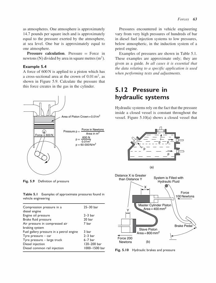
Forces 63
as atmospheres. One atmosphere is approximately14.7 pounds per square inch and is approximatelyequal to the pressure exerted by the atmosphere,at sea level. One bar is approximately equal toone atmosphere.
Pressure calculation. Pressure = Force innewtons (N) divided by area in square metres (m2).
Example 5.4A force of 600 N is applied to a piston which hasa cross-sectional area at the crown of 0�01 m2, asshown in Figure 5.9. Calculate the pressure thatthis force creates in the gas in the cylinder.
Force = 600 N
Area of Piston Crown = 0.01m2
Pressure p =Force in Newtons
Area in m2
p =
p = 60 000 N/m2
600 N0.01m2
Fig. 5.9 Definition of pressure
Table 5.1 Examples of approximate pressures found invehicle engineering
Compression pressure in adiesel engine
25–30 bar
Engine oil pressure 2–3 barBrake fluid pressure 20 barAir pressure in compressed airbraking system
7 bar
Fuel gallery pressure in a petrol engine 3 barTyre pressure – car 2–3 barTyre pressure – large truck 6–7 barDiesel injection 120–200 barDiesel common rail injection 1000–1500 bar
Pressures encountered in vehicle engineeringvary from very high pressures of hundreds of barin diesel fuel injection systems to low pressures,below atmospheric, in the induction system of apetrol engine.
Examples of pressures are shown in Table 5.1.These examples are approximate only; they aregiven as a guide. In all cases it is essential thatthe data relating to a specific application is usedwhen performing tests and adjustments.
5.12 Pressure inhydraulic systems
Hydraulic systems rely on the fact that the pressureinside a closed vessel is constant throughout thevessel. Figure 5.10(a) shows a closed vessel that
System is Filled withHydraulic Fluid
Force100 Newtons
(b)
Brake Pedal
Force 200 Newtons
Master Cylinder PistonArea = 400 mm2
X
Slave PistonArea = 800 mm2
Y
Distance X is Greaterthan Distance Y
p
(a)
p p
p
Fig. 5.10 Hydraulic brakes and pressure

64 Automotive science and mathematics
has a number of pistons located in it. The pressureon each piston (not the force) is equal.
Example 5.5Figure 5.10(b) shows the basic structure of ahydraulic braking system.
The pressure at the master cylinder =100 N
400 mm2= 0�25 N/mm2 = 2�5 bar
This is also the pressure at the slave cylinder.The force at the slave cylinder = pressure ×
area = 2�5 N/mm2 ×800 mm2 = 200 N.
5.13 Hooke’s law
Figure 5.11(a) shows a simple apparatus that isused to demonstrate the effect of force applied toan elastic body. In this case the elastic body is ametal coil spring. The spring is suspended froma secure support and at its lower end there is aweight container to which various weights maybe added and removed. A pointer is attached tothe lower end of the spring and this permits read-ings of spring extension to be recorded as weightsare added. When a series of weights and corre-sponding spring extension have been recorded, theweights are removed and the spring will return toits original unloaded length.
A typical set of results for this type of demon-stration are shown in the table in Figure 5.9(b)and, when these are plotted on squared paper,they produce a straight-line graph as shown inthe figure. This result shows that the extension isdirectly proportional to the load producing it. Thisis known as Hooke’s law and it is named afterRobert Hooke (1635–1703).
The relationship between load and extensionis known as the stiffness of the spring, or thespring rate. Expressed mathematically, stiffness =load/extension.
When the spring is in compression, stiffness =load/compression.
Weights
Scale
Fixed Support
(a)
24
20
16
12
8
4
0
Ext
ensi
on m
m
10 20 30 40 50 60
Load Newtons
Hooke’s Law Coil Spring
(b)
10 20 30 40 50 60
4 8 12 16 20 24
LoadN
Extensionmm
Spring Rate = LoadExtension
Fig. 5.11 Hooke’s law apparatus and results

Forces 65
Example 5.6A front suspension spring of a certain vehicle iscompressed by 30 mm when it carries a load of240 N. Calculate the spring stiffness (rate).
SolutionCalculate the spring stiffness (rate).
Spring stiffness = loadcompression
240/30 = 8 N/mm
5.14 Practicalapplications
Figure 5.12 shows one of the many automotiveapplications where factors relating to spring rateare likely to be encountered.
Valve spring rate is critical in ensuring thevalves operate correctly. Valve springs can dete-riorate in service and the dimensions shown herecan be used to check that valve springs are suitablefor further use.
The type of equipment used for testing valvesprings is shown in Figure 5.12.
The force applied to the spring is shown onthe dial gauge and a calibrated scale to the right,under the operating handle, indicates the amountof spring compression.
5.15 Summary
Hooke’s law: Within the elastic limit for a materialthe extension produced is directly proportional tothe load producing it.
Stiffness of a spring = forceextension
Pressure = forcearea
Pressure units: 1 N/m2 =1 Pa (pascal).1 bar = 105 N/m2
The hydraulic pressure inside a closed containeris constant throughout the container.
5.16 Exercises
5.1 In order to carry out work on a front sus-pension system, a spring compressor isused to compress the spring axially by250 mm. The spring rate is 9 N/mm.
Is the spring force that is held back bythe spring compressor:(a) 2250 N(b) 27.8 N(c) 225 kN(d) 278 N
5.2 The coil spring in a ball and spring typeof oil pressure relief valve exerts a forceof 24 N on the ball valve when it is com-pressed by 8 mm. Is the spring rate:(a) 192 N/mm(b) 30 N/mm
Spring Balance
P
CalibratedScale
SpringLength
PForce
0
350 N
900 N
43.2 mm
37.0 mm
26.6 mm
Fig. 5.12 Testing a valve spring

66 Automotive science and mathematics
(c) 3 N/mm(d) 0.33 N/mm
5.3 Might a weak spring in an oil pressure reliefvalve cause(a) the oil pressure at normal engine run-
ning speed to be too low?(b) the oil pressure at normal engine run-
ning speed to be too high?(c) not cause any difference in the oil
pressure?(d) the effect can be overcome by fitting a
new oil pump?5.4 Find the magnitude and direction of the
resultant of the two forces A and B shownin Figure 5.13. What alteration is requiredto be made to this resultant in order to makeit become the equilibrant of the two forcesA and B?
45°
80 N
B
60°130 N
A
Fig. 5.13 Calculation of forces (Exercise 5.4)
5.5 Two forces OA and OB of 50 N and 70 Nrespectively, pull on a body at point O. Theangle AOB is 70�. Find the magnitude anddirection of the third force acting at pointO that will balance the other two forces.
5.6 State Hooke’s law. A compression springhas a stiffness of 40 kN/m. Calculate (a) theamount of compression when a force of280 N is applied to the spring, (b) the forcerequired to compress the spring 5 mm.
5.7 When a vehicle is being lifted by a craneas shown in Figure 5.14 the force F, inthe lifting cable, is producing two effects.One effect is to attempt to lift the vehicle
40°
F = 5 kN
Fig. 5.14 Vertical and horizontal components of a force
in a vertical direction and the other is toattempt to move the vehicle in a horizontaldirection. Use a force diagram to determinethe magnitude of the horizontal componentof force F.
5.8 Find the forces in the jib and the tieof the wall mounted crane shown inFigure 5.15(a).
5.9 Find the side thrust F acting on the cylinderwall of the engine mechanism shown inFigure 5.15(b).
(a)
Tie
Jib
3T
60°
30°
(b)
30°
F
2000 N
Fig. 5.15 Calculations (Exercises 5.8–5.11)

Forces 67
(d)
PN QN
28°
2 kN
40°
(c)
45°
A B
45°
30°
50 N
Fig. 5.15 Continued
5.10 Three coplanar forces are acting at a pointas shown in Figure 5.15(c). Determine thesizes of forces A and B.
5.11 A 2 kN weight is suspended from two ropesas shown in Figure 5.15(d). Determine thesizes of forces P and Q�
5.12 A certain petrol engine piston crown hasa cross-sectional area of 0�012 m2. If thecompression force on the piston is 30 kN,calculate the pressure acting on the pistoncrown.
15.13 If the gravitational constant is 9�81 m/s2, isthe gravitational force acting on a vehicleof 1 tonne mass:(a) 981 kg(b) 98.1 N(c) 9.81 kN(d) 981 N
15.14 Is an object whose centre of gravity riseswhen a force is applied and falls backto its original position when the force isremoved:(a) in unstable equilibrium?(b) in stable equilibrium?(c) in neutral equilibrium?(d) lacking in stability?

6Materials – Stress, strain, elasticity
6.1 Introduction
Many of the materials that are used in motor vehi-cle engineering are elastic, that is to say that theychange shape under load and then return to theiroriginal shape when the load is removed. Elas-ticity is one of the properties that allow mate-rials and components to experience much stressand strain during their working lives. For exam-ple, coil springs used in suspension systems com-press under load and then expand when the loadis removed; this type of action occurs thousandsof times and the springs are expected to func-tion properly for many years. Other componentssuch as bolts, cables, rods, etc., experience equallysevere operating conditions but the elastic effectis not so obvious. A change of dimensions calledstrain occurs when materials are stressed; forexample when a cylinder head bolt is tightened toits final torque the bolt will stretch a little. Muchof the energy that is used to tighten the bolt isstored as strain energy in the bolt and it is thisenergy that gives rise to the force that clamps thecylinder head in position. When the cylinder headbolts are released (undone) the strain energy isreleased and the bolt returns to its original sizebecause the material is elastic. However, if the boltis over-tightened, the bolt may stretch or break. Infact it will most probably stretch first. To see why
this is so it is useful to have an insight into someof the basics about the behaviour of materials.
6.2 Stress
Forces that tend to stretch, or pull something apart,are known as tensile forces and they produce twoimportant effects:
1. In trying to pull the bolt apart, internal resistingforces are created and these internal forces areknown as stress.
2. The length of the bolt will increase, and thischange in the bolt’s dimensions is known asstrain.
Stress is calculated by dividing the applied forceby the cross-sectional area of the bolt.
Stress = ForceCross-sectional area
(6.1)
Types of stressThere are three basic forms of stress:
1. tensile stress;2. compressive stress;3. shear stress – torsional stress is a form of shear
stress.

Materials – Stress, strain, elasticity 69
Shear
Compression
Tension
Fig. 6.1 The three basic stresses
Examples of the three basic stressesin automotive componentsFigure 6.2(a) shows a cylinder head bolt. This isa component that is highly stressed in tension.
Figure 6.2(b) shows a piston and connecting rodassembly. On the compression and power strokesthe connecting rod is subject to large compressivestress. The gas force on the gudgeon pin attemptsto shear the pin on each side of the small endof the connecting rod. In this case the gudgeonpin is said to be in double shear because twocross-sectional areas are subject to the shearingforce.
6.3 Tensile test
In materials testing, a standard size specimen ofsteel is stretched in a tensile testing machine untilit breaks. During the test, the applied force and thecorresponding extension are recorded. Figure 6.3shows a typical graph obtained during a tensiletest on a steel specimen.
The graph shows that up to point A the exten-sion is proportional to the load; this is the elasticlimit, or limit of proportionality. After point A,
Cylinder Head Bolt
(b)
(a)
Tensile Stress
CompressiveStress
Shear Stress
GudgeonPin
ConnectingRod
Fig. 6.2 Components under stress
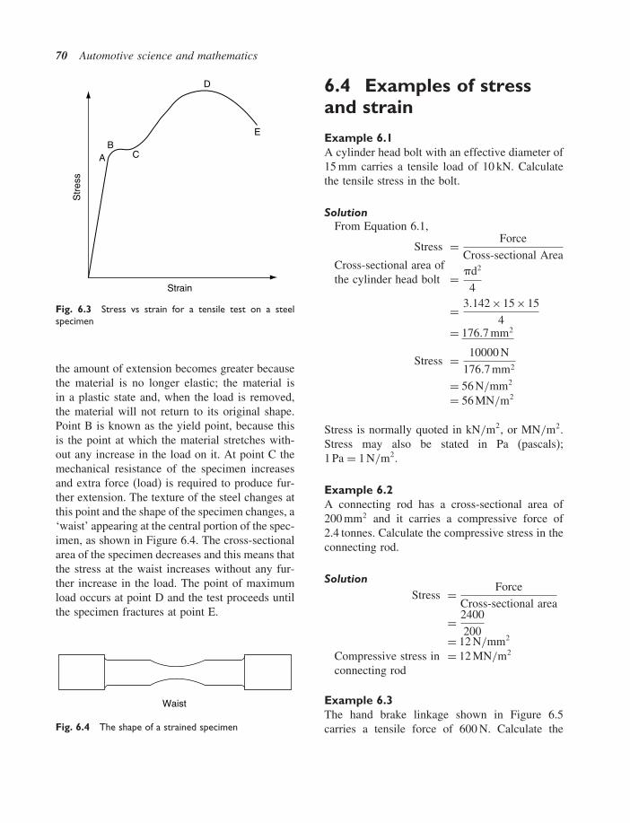
70 Automotive science and mathematics
AB
C
D
E
Strain
Str
ess
Fig. 6.3 Stress vs strain for a tensile test on a steelspecimen
the amount of extension becomes greater becausethe material is no longer elastic; the material isin a plastic state and, when the load is removed,the material will not return to its original shape.Point B is known as the yield point, because thisis the point at which the material stretches with-out any increase in the load on it. At point C themechanical resistance of the specimen increasesand extra force (load) is required to produce fur-ther extension. The texture of the steel changes atthis point and the shape of the specimen changes, a‘waist’ appearing at the central portion of the spec-imen, as shown in Figure 6.4. The cross-sectionalarea of the specimen decreases and this means thatthe stress at the waist increases without any fur-ther increase in the load. The point of maximumload occurs at point D and the test proceeds untilthe specimen fractures at point E.
Waist
Fig. 6.4 The shape of a strained specimen
6.4 Examples of stressand strain
Example 6.1A cylinder head bolt with an effective diameter of15 mm carries a tensile load of 10 kN. Calculatethe tensile stress in the bolt.
SolutionFrom Equation 6.1,
Stress = ForceCross-sectional Area
Cross-sectional area ofthe cylinder head bolt = �d2
4
= 3�142×15×154
= 176�7 mm2
Stress = 10000 N176�7 mm2
= 56 N/mm2
= 56 MN/m2
Stress is normally quoted in kN/m2, or MN/m2.Stress may also be stated in Pa (pascals);1 Pa = 1 N/m2.
Example 6.2A connecting rod has a cross-sectional area of200 mm2 and it carries a compressive force of2.4 tonnes. Calculate the compressive stress in theconnecting rod.
SolutionStress = Force
Cross-sectional area
= 2400200= 12 N/mm2
Compressive stress inconnecting rod
= 12 MN/m2
Example 6.3The hand brake linkage shown in Figure 6.5carries a tensile force of 600 N. Calculate the

Materials – Stress, strain, elasticity 71
Clevis Pin Double Shear
Shear Areas
Fig. 6.5 Clevis pin in double shear (Example 6.3)
shear stress in the clevis pin, which is 12 mm indiameter.
In this case the shearing action is attempting toshear the clevis pin across two cross-sectional areas.
The cross-sectional areof the clevis pin = � ×12×12
4
= 3�142×12×124
= 113�1 mm2
In this case the shearing action is attempting toshear the clevis pin across two cross-sectionalareas. The area resisting shear = 2×113�1
= 226�2 mm2
Shear stress = forcearea resisting force
= 600226�2
= 2�65 N/mm2
Shear stress inclevis pin = 2�65 MPa
Example 6.4A propeller shaft coupling of a truck is secured byfour bolts of 14 mm diameter that are equally spacedat a radius of 50 mm from the centre of the pro-peller shaft. Calculate the shear stress in each boltwhen the shaft is transmitting a torque of 500 N m.
SolutionFigure 6.6 shows the layout of the coupling flange.
Torque transmitted by propellershaft T = 500 N m
Force = TR
14 mm dia.
100 m
m
Fig. 6.6 Propeller shaft coupling flange (Example 6.4)
Radius at which force acts = 50 mm
∴ F = 500 N m0�05 m
= 10 000 N
This force is evenly shared by the four couplingbolts
(csa = cross-sectional area)
Force on each bolt = 10 0004
= 2500 N
Shear stress in each bolt = Forcecsa
csa of bolt = � ×0�014×0�0144
= 0�000154 m2
Stress = 25000�000154
= 16�23 MN/m2
Stress in each coupling bolt = 16�23 MN/m2
6.5 Stress raisers
Sharp corners and notches of the type shown inFigure 6.7 cause regions of high stress that canlead to component failure. These stress raisers can

72 Automotive science and mathematics
(b)
Crankshaft
Sharp Corner – IncorrectStress Raiser
(c)
Journal
Radius – Correct
(a)
Cuts – Incorrect
Connecting Rod
StressRaiser
Fig. 6.7 Stress raisers
be caused by bad repair practices such as plac-ing saw cuts to identify a component, incorrectmachining when regrinding a crankshaft, drillingholes in components when fixing attachments tosome part of a vehicle, etc.
6.6 Strain
When a load is applied to a metal test bar a changeof shape takes place. A tensile load will stretch thebar and a compressive load will shorten it. Thischange of shape is called strain. The three basictypes of strain are shown in Figure 6.8.
PP
P B
A
x
x
l
(a) (b)Tensile
Strain = x /l Strain = x /lCompressive
(c)
Strain = x /l = Angle φ in RadiansShear
φ
x
l l
Fig. 6.8 The three types of strain
Tensile or compressive strain
= change in lengthoriginal length
(6.2)
Example 6.4A steel rod 200 mm in length stretches by 0.12 mmwhen it is subjected to a tensile load of 2 tonnes.Determine the strain.
Solution
Strain = change in lengthoriginal length
= 0�12 mm200 mm
Tensile strain in the steel rod = 0�0006
Note: strain does not have any units.
Shear strainFigure 6.8c shows a rectangular block of materialto which a shearing force P is applied. The bottomedge of the rectangular block is secured to animmovable surface. The action of force P causesthe top edge of the block to move a distance xin the direction of force P, which makes the edgeAB take up an angle of � radians. This angle isused as the measure of shear strain.

Materials – Stress, strain, elasticity 73
6.7 Elasticity
Stress, strain, elasticityIn terms of stress and strain, Hooke’s law statesthat the strain produced in an elastic material isdirectly proportional to the stress that produces it.
Expressed mathematically this means that
stressstrain
= constant
This constant is known as the modulus of elas-ticity, or Young’s modulus. The symbol E is nor-mally used to denote modulus of elasticity.
For tensile or compressive stress E = stressstrain
(6.3)
For shear stress the term modulus of rigidity isused and this is represented by the symbol G.
For shear stress G = stressstrain
(6.4)
Example 6.5Determine the extension of a metal rod of 14 mmdiameter and 200 mm length when it is placedunder a tensile load of 2 tonnes. Take g = 10 m/s2.The modulus of elasticity E for the material =200 GN/m2.
Solution
Cross-sectional area
(csa) of the rod = �d2
4
= 3�142×14×144
csa = 154 mm2
stress = loadcsa
= 2000×10154
= 129�8 N/mm2
Stress = 129�8 MN/m2
E = stressstrain
Table 6.1 Typical approximate values for Young’smodulus
Material Young’s modulus(E) GN/m2 (GPa)
Cast iron 110Copper 117Aluminium 71Mild steel 210Magnesium 44Phosphor bronze 120Nickel alloy 110
Strain = stressE
= 129�8×10⁶
200×109
= 0�649×10−3
strain = extensionoriginal length
Extension = strain ×original length
= 0�649×10−3 ×200 mm
Extension = 0�13 mm
Some typical approximate values for E are shownin Table 6.1.
6.8 Tensile strength
The tensile strength of a material is the maximumtensile stress that the material can bear beforebreaking.
Tensile strength = maximum loadoriginal csa of the material
(6.5)(csa = cross-sectional area)
Example 6.6Determine the tensile strength of a 15 mm diame-ter steel rod that is able to withstand a maximumtensile load of 74 kN.

74 Automotive science and mathematics
Solution
Crosss-sectional area of rod = �d2
4= 0�7854 ×
0�015×0�015 = 0�0001767 m2
Tensile load = 74 kN
Tensile strength = maximum loadoriginal csa of the material
= 74×10000�0001767
= 419 MN/m2
6.9 Factor of safety
In order to preserve the strength and workingproperties of a component, the maximum load towhich a material is subjected is restricted to afigure which is below the tensile strength of thematerial. This maximum working load gives riseto the allowable working stress and it is a fractionof the tensile strength of the material.
The allowable working stress = tensile strengthfactor of safety
(6.6)
Example 6.7A steel tie rod in a suspension system is designedwith a factor of safety of 6. The tensile strength ofthe steel is 420 MN/m2. Calculate the allowableworking stress.
Solution
Allowable working stress = tensile strengthfactor of safety
= 420 MN/m2
6
= 70 MN/m2
6.10 Torsional stress
The twisting action that arises when torque isapplied to an object such as a shaft gives rise
to shear stress. The following formula relates thevarious factors involved when torque is applied toa shaft.
TJ
= G�
lR= fs (6.7)
Where T (in N m) is the torque applied to the shaft,J is the polar moment of inertia which is derivedfrom the dimensions of the shaft (this is in m4),G is the modulus of rigidity in N/m2, l is thelength of the shaft in metres, fs is the shear stressin N/m2� � is the angle of twist in radians, and Ris the radius where the stress is greatest, normallythe outer radius of the shaft.
Example 6.8A solid steel shaft of 20 mm diameter and 200 mmlength is subjected to a torque of 220 N m. If Jfor the shaft = 1�57×10−8m4, calculate the shearstress.
Solution
fs
R= T
J
fs = T ×RJ
= 220 N m ×0�010 m1�57×10−8 m4
= 140 MN/m2
Shear stress produced by 220 N m torque =140 MN/m2
Table 6.2 Modulus of rigidity G (shear modulus)
Material Approx. values of modulus ofrigidity (G) in GPa
Steel 80Copper 25Aluminium alloy 20–30

Materials – Stress, strain, elasticity 75
6.11 Strain energy
When a force is applied to an elastic component,such as steel spring or a bolt, a change in shapeoccurs. In the case of a tensile force, the changeof shape will be in the form of an increase in thelength of the component. The force has movedthrough a distance, which means that work hasbeen done. As the force (weight) increases, theextension increases proportionately and the forceversus distance graph has the shape shown inFigure 6.9.
W NewtonsForce
Ext
ensi
on
x m
Area = Work Done = Strain Energy
Area = ½ Wx N m
Fig. 6.9 Strain energy
The work done in stretching the spring = areaunder the graph
Strain energy = 1/2 Wx N m (6.8)
Where W = the maximum force in newtons andx = extension of spring in metres.
Example 6.9Determine the strain energy stored in a valvespring that is compressed by 15 mm under a loadof 750 N.
Solutionx = 0�015 m
W = 750 N
Strain energy = Wx
2
= 750×0�0152
= 5�625 N m
= 5�625 J
6.12 Strength ofmaterials
For practical purposes, components are designedto withstand forces and loads that a device isdesigned for and, so long as the instructions foruse and maintenance, such as safe loads and tight-ening torques, are observed, problems should notbe experienced.
6.13 Other terms usedin describing materials
HardnessA hard material is one that resists indentation orabrasion by another material. The Brinell test is onemethod that is used to measure hardness and it oper-atesbypressingahardenedmetal carbide ball undera standard load into the surface of the specimen.The dimensions of the impression made are usedto calculate the Brinell Hardness Number (BHN).
HardeningSteels that contain 3% carbon or above may be hard-ened by heating them to a temperature of approxi-mately 750�C (cherry red) and then quenching themin cold water. The temperature for this processvaries according to carbon content. When quench-ing in cold water is considered too severe the steelis quenched in special quenching oil.

76 Automotive science and mathematics
TemperingTempering is the process of reheating hardenedsteel to a temperature below the critical range, inorder to reduce the hardness.
AnnealingThis involves heating the material to a suitabletemperature and holding it at that temperature fora suitable period before allowing it to cool. Thepurpose is to soften the material, improve theworking properties, and reduce internal stressesafter working.
Case hardeningCase hardening is a process that is used to impart ahard surface to steel. It is used in components thatrequire a surface that is resistant to wear whilstretaining a tough inner structure. A crankshaft isan example of a component that is normally casehardened on the crankpins and journals. A processthat is used in the manufacture of some crankshaftsis known as nitriding. In nitriding, special typesof steel are heated to approximately 520�C in anatmosphere of gaseous ammonia to produce a hardsurface of approximately 0.5 mm depth.
ToughnessA material is said to be tough when a large amountof energy is required to fracture it.
BrittlenessMaterials that break without undergoing local dis-tortion and are unable to withstand sharp blows aresaid to be brittle. Most types of cast iron are brittle.
DuctilityA material that can be drawn out by tensile force issaid to be ductile. The steel sheet that is used in theconstruction of motor car panels is of a type knownas deep drawing steel and this is a ductile material.
MalleabilityMetals that can hammered and bent without crack-ing are said to be malleable. Lead is an exampleof a malleable material.
6.14 Non-ferrous metals
These are mainly alloys that contain no iron. Com-monly used non-ferrous alloys are those madefrom copper, lead, tin, aluminium or magnesium.Non-ferrous alloys are used extensively in auto-motive engineering.
6.15 Non-metallicmaterials
Synthetic materials, commonly known as plastics,are readily formed into quite intricate shapes andthis makes them suitable for many applicationsin motor vehicle construction. In general, plasticsare resistant to corrosion and a range of plasticshave been developed to suit many applications onvehicles where metals were once used. Plastics aresometimes described as thermosets, which meansthat the plastic does not soften when re-heated, orthermoplastic, which means that the plastic doessoften when re-heated.
KevlarKevlar is the DuPont trade name for a syntheticmaterial that is formed from high-strength aramidfibres. It has tensile strength equivalent to that ofsteel, it is lighter than steel and it is resistant tocorrosion (see Table 6.3).
Table 6.3 Some properties of Kevlar
Material Density �kg/m3) Tensile strength�GN/m2�
Kevlar 49 1440 3.1Steel piano wire 7860 3.0

Materials – Stress, strain, elasticity 77
6.16 Recycling ofmaterials
Disposal of vehicles that have reached the end oftheir useful lives is a factor that has received muchattention in recent years. Steel, copper, lead andother metallic materials are often recycled manytimes and in most areas facilities exist for deal-ing with them. Other materials are dealt with byspecial processing methods and facilities for deal-ing with all vehicle materials are being developedboth locally and nationally in the UK. Vehiclesthat have reached the end-of-life stage are knownas end-of-life vehicles (ELVs).
6.17 Summary of mainformulae
Stress = ForceCross-sectional area
Tensile or compressive Strain = Change in lengthOriginal length
For tensile or compressive stress, E = stressstrain
For shear stress G = stressstrain
Tensile strength = maximum loadoriginal csa of the material
The allowable working stress = tensile strengthfactor of safety
For torsionTJ
= G�
l= fs
R
Strain energy = ½ Wx N m
The polar moment of inertia J = �d4
32for a solid
shaft
J = � �D4 −d4�
32for a hollow shaft
6.18 Exercises
6.1 A steel bolt with an effective diameter of12 mm and length of 50 mm carries a tensileload of 10 kN. Calculate the extension inlength of the bolt under this load, given thatE = 200 GN/m2.
6.2 (a) Define ‘strain’, ‘stress’, ‘modulus ofelasticity’.
(b) A steel tie rod used in a suspension sys-tem is 400 mm long with a diameter of15 mm. Determine the stress in the tierod when a tensile force of 600 N isapplied to it under braking.
(c) If E for the rod = 200 GN/m2 calculatethe extension of the rod caused by thisforce.
6.3 The shackle pin in a certain leaf spring hasa diameter of 18 mm. When the vehicle isfully loaded the shackle pin carries a load of2.5 tonnes. Calculate the shear stress in theshackle pin. Take G = 10 m/s2.
6.4 An axle shaft 0.5 m long is subjected toa torque of 1200 N m. Given that thepolar moment of inertia J for the shaft =0�000041 m4, calculate the angle of twist inthe shaft. Take the modulus of rigidity G =85 GN/m2.
6.5 A piston and connecting rod assembly car-ries a direct gas force of 8 kN at the top deadcentre position. The gudgeon pin is hollowwith an outside diameter of 18 mm and aninternal diameter of 12 mm if the minimumcross-sectional area of the connecting rod is300 mm2.Calculate:(a) the stress in the gudgeon pin;(b) the stress in the connecting rod.
6.6 A certain engine has a bore diameter of100 mm. The gudgeon pin has an outsidediameter of 20 mm and an inside diameter of14 mm. If the cylinder gas pressure is 10 barat the top dead centre position, calculate thestress in the gudgeon pin.
6.7 A truck engine develops a maximum torqueof 400 N m. The lowest gearbox ratio is 8.5:1

78 Automotive science and mathematics
and the drive axle ratio is 5:1. When in thelow gear the transmission efficiency is 90%.Given that the final drive axle shafts are40 mm in diameter, calculate the shear stressin each axle shaft when transmitting maxi-mum torque; the drive is equally balancedon each side of the differential gear.
For the axle shafts J = �d4
32.
6.8 Determine the maximum torque that can betransmitted by a propeller shaft if the max-imum permissible shear stress is limited to15 MPa. The outside diameter of the shaft =50 mm and the polar moment of inertia J forthe shaft = 2�62×10−7m4.
6.9 Give three examples in each case of vehiclecomponents that are subjected to the follow-ing: (a) shear stress; (b) tensile stress; (c)compressive stress.
Calculate the tensile force on a bolt 15 mmin diameter when the tightening torque pro-duces a tensile stress of 60 MPa.
6.10 The figures in Table 6.4 were recorded inan experiment to determine the value ofYoung’s modulus of elasticity for a steelwire. Plot a graph with extension on the
Table 6.4 Calculation of Young’s modulus(Exercise 6.10)
Tensile force applied to thewire (N)
Extension (mm)
20 0.340 0.660 0.880 1.1100 1.4120 1.7140 2.0160 2.2180 2.5200 2.8220 3.3
horizontal axis and select a suitable point onthe graph that will enable you to select val-ues of load and extension from which to cal-culate Young’s modulus. Calculate Young’smodulus of elasticity for the steel wire.Initial length of wire = 1.8 mInitial diameter of wire = 1 mm
6.11 An air brake actuator has a diaphragm of120 mm diameter. The clevis pin that trans-mits the braking force from the diaphragmrod to the brake lever has a diameter of15 mm. Calculate the stress in the clevis pinwhen the air pressure on the diaphragm is6 bar.
Air Pressure
Rod Diameter 15 mm
Air Brake Actuator
Fig. 6.10 Strain energy
6.12 The diaphragm in a vacuum servo has aneffective area of 0�03 m2. Under certain con-ditions the pressure difference a between thevacuum side of the servo and the air pressureside is 50 kPa.
Calculate (a) the force that the servodiaphragm exerts on the master cylinderpush rod, and (b) the stress in the masterpush rod that has a diameter of 10 mm, underthese conditions.
6.13 Calculate the maximum power that can betransmitted by a tubular propeller shaft at4200 rev/min if the shear stress is not toexceed 20 MN/m2. The outer diameter ofthe shaft is 50 mm and the inner diameter is44 mm.

7Levers and moments, torqueand gears
7.1 Levers
Leverage and the use of levers occurs in the useof tools such as spanners, pry bars, pliers etc., andin many vehicle mechanisms such as clutch andbrake pedals, throttle linkages and suspension units.
7.2 Principles of leverage
The basic principles of leverage are covered by arule that is known as the principle of moments.
7.3 The principle ofmoments
The moment of a force is defined as the productof the force and the perpendicular distance fromthe fulcrum to the line in which the force is acting.
Example 7.1In this example (see Figure 7.1) a beam that is80 cm long rests on a pivot (fulcrum) that is 20 cmfrom one end. There are forces of 60 newtons and20 newtons acting at right angles to the beam,as shown. This system of a beam, the forces and
the fulcrum are in equilibrium, i.e. the beam andforces are balanced about the fulcrum. When abeam is in equilibrium like this, the principleof moments states that the clockwise momentsabout the fulcrum are equal to the anti-clockwisemoments about the fulcrum.
In this case the clockwise moment is equal to
20 N ×60 cm = 1200 N cm
And the anti-clockwise moment is equal to
60 N ×20 cm = 1200 N cm
For convenience the clockwise moment is oftenabbreviated to CWM and the anti-clockwisemoment to ACWM.
According to the principle of moments, the sim-ple beam problem shown in Figure 7.1 may bewritten as:
CWM = ACWM
60 N ×20 cm = 20 N ×60 cm
1200 N cm = 1200 N cm
In simple lever problems it is usual to be given thesize of one force and both distances, and then tobe required to work out the size (magnitude) of theother force, as shown in the following example.
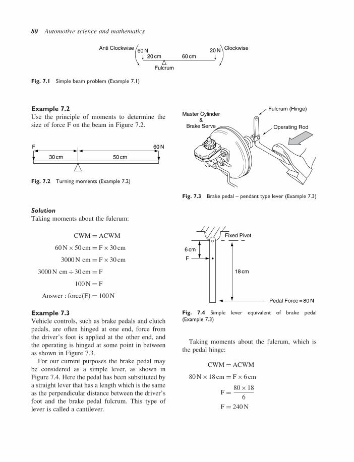
80 Automotive science and mathematics
Fulcrum
20 cm 60 cm60 N 20 N ClockwiseAnti Clockwise
Fig. 7.1 Simple beam problem (Example 7.1)
Example 7.2Use the principle of moments to determine thesize of force F on the beam in Figure 7.2.
30 cm 50 cm
F 60 N
Fig. 7.2 Turning moments (Example 7.2)
SolutionTaking moments about the fulcrum:
CWM = ACWM
60 N ×50 cm = F ×30 cm
3000 N cm = F ×30 cm
3000 N cm ÷30 cm = F
100 N = F
Answer � force�F� = 100 N
Example 7.3Vehicle controls, such as brake pedals and clutchpedals, are often hinged at one end, force fromthe driver’s foot is applied at the other end, andthe operating is hinged at some point in betweenas shown in Figure 7.3.
For our current purposes the brake pedal maybe considered as a simple lever, as shown inFigure 7.4. Here the pedal has been substituted bya straight lever that has a length which is the sameas the perpendicular distance between the driver’sfoot and the brake pedal fulcrum. This type oflever is called a cantilever.
Master Cylinder&
Brake Serve
Fulcrum (Hinge)
Operating Rod
Fig. 7.3 Brake pedal – pendant type lever (Example 7.3)
Pedal Force = 80 N
18 cm
6 cm
F
Fixed Pivot
Fig. 7.4 Simple lever equivalent of brake pedal(Example 7.3)
Taking moments about the fulcrum, which isthe pedal hinge:
CWM = ACWM
80 N ×18 cm = F ×6 cm
F = 80×186
F = 240 N

Levers and moments, torque and gears 81
7.4 The bell crank lever
The bell crank lever, as shown in Figure 7.5, isused in many vehicle systems and the principleof moments may be applied to the solution ofnumerical problems associated with it.
When the bell crank lever is in equilibrium(balanced), the clockwise turning moment aboutthe fulcrum (pivot) is equal to the anti-clockwisemoment about the fulcrum. It is important to notethat the turning moment is the product of the forceand the perpendicular distance from the fulcrumto the line in which the force is acting. This isan important point to note because when a givenforce is applied at an angle other than at a rightangle it produces a smaller turning moment.
In Figure 7.5 the distances of the forces fromthe fulcrum are the perpendicular distances, so theturning moments are:
CWM = ACWM
18 N ×10 cm = 15 N ×12 cm
180 N cm = 180 N cm
10 cm
12 cm
18 N
180 N cmClockwise
180 N cmAnti Clockwise
15 N
Fulcrum
Fig. 7.5 A bell crank lever
A practical application of thebell crank leverThe handbrake lever shown in Figure 7.6 is hingedon the fulcrum pin. A force applied by hand atthe operating end causes that end of the lever tomove upwards and this results in forward move-ment of cable that applies the brakes at the rear
Handbrake Lever
Fulcrum Pin1
2
Fig. 7.6 Handbrake lever
wheels. An adjustment is provided to compensatefor wear. Should the movement on the handbrakelever become excessive it becomes increasinglydifficult to apply the hand operating force at rightangles to the lever and this leads to a weakeningof the pull that is exerted on the handbrake cable.
35 cm
Hand Force
Fulcrum Pin
5 cm
To Brakes
Fig. 7.7 Skeleton lever – handbrake (Example 7.4)
For purposes of calculation, the mechanics ofthe handbrake lever can be represented by a skele-ton bell crank lever, as shown in Figure 7.7.
Example 7.4In the handbrake lever mechanism shown inFigures 7.6 and 7.7, a brake cable force of 420 N

82 Automotive science and mathematics
is required to apply the brakes. Calculate the handforce, applied at right angles to the long part ofthe lever, that is required to produce this force inthe cable.
Applying the principle of moments gives:
CWM = ACWM
F ×35 cm = 420 N ×5 cm
F = 420×535
F = 60 N
A force of 60 N is required at the operating endof the handbrake lever.
Example 7.5Figure 7.8 shows a horizontal beam that is sup-ported at each end. The loads on the beam are intonnes and the distances between the loads are inmillimetres. Determine the size of the reactionsR1 and R2 at the supports.
600
2T 3T 2T
400 700 300
R1 R2
Fig. 7.8 Simply supported beam (Example 7.5)
Take moments about the right-hand support:
CWM = ACWM
R1 ×2000 = �2×300�+ �3×1000�+ �2×1400�
R1 = 64002000
R1 = 3�2 tonnes
Because the beam is in equilibrium the upwardforces are equal to the downward forces so R2 isfound by subtracting R1 from the total downwardforce:
R2 = 7−3�2 = 3�8 tonnes
7.5 Axle loadings
Example 7.6Figure 7.9 shows a vehicle of total weight = 1.4tonnes. The wheelbase of the vehicle is 2.5 m andthe centre of gravity is positioned 1.2 m behindthe centre of the front axle.
1.4 Tonne
C of G
2.5 m
1.2 m 1.3 m
RF RR
Fig. 7.9 Axle loadings (Example 7.6)
The principle of moments may be used to deter-mine the axle loadings Rf and Rr.
Take moments about Rf :
CWM = ACWM
1�4×1�2 = Rr ×2�5
Rr = 1�4×1�22�5
Rr = 0�672 tonne
The total weight pushing down = forcepushing up
1�4 tonnes = 0�672 tonne +Rf
Rf = 1�4−0�672
Rf = 0�728 tonne
The axle loadings are: front axle 0.728 tonne, rearaxle 0.672 tonne.

Levers and moments, torque and gears 83
7.6 Torque
Torque is a turning effect; a clear demonstrationof the meaning of torque may be seen in thewidely used torque wrench that is used for tight-ening nuts and bolts to a preset value, as shownin Figure 7.10.
Torque is the product of force and perpendiculardistance from the centre of rotation to the line inwhich the force is acting.
Fig. 7.10 Torque wrench
Example 7.7In the example of the torque wrench, the torquemay be calculated as follows.
Assume that the hand force is applied at rightangles to the shaft of the torque wrench and thatthe force is applied at a distance of 40 cm fromthe centre of the axle. In this particular case thetorque required is 25 N m. Calculate the force Frequired to produce this amount of torque. (SeeFigure 7.11.)
In this case we have: torque (T) = 25 N m;radius (R) = 40 cm = 0.4 m.
T = F ×R
F = T ÷R
F = 25 N m0�4 m
F = 62�5 N
Handle of Torque Wrench
40 cm
Centre of Hub FHandforce
FN × 0.4 m = 25 N m
F = 25 N m
= 62.5 N0.4 m
Fig. 7.11 Torque calculation (Example 7.7)
7.7 Engine torque
Engine torque is produced by the action of thegas force on the piston which is transmitted tothe crankshaft through the connecting rod. Theprinciple is shown in Figure 7.12.
Example 7.8In this case, the effective force on the connect-ing rod is 2000 N and the connecting rod ismaking a right angle with respect to the crankthrow. The throw (radius) of the crank is 60 mm.The connecting rod is at a right angle to thecrank throw.
Here, the torque produced is:
Torque (T) = Force (F)×Radius R
F = 2000 N, R = 60 mm = 0�06 m
T = F ×R
T = 2000 N ×0�06 m
T = 120 N m
Crankshaft torque T = 120 N m
It is important to note that the torque is cal-culated from the force and the perpendicular dis-tance from the centre of rotation to the line inwhich the force is acting.

84 Automotive science and mathematics
Piston
Force in Connecting Rod = 2000 N = 2 kN
Connecting Rod
DOR
Crank
60 mm
Radius of Crank = 60 mm = 0.06 m.The Connecting Rod Force is at Right Angles to the Crank Throw.
Torque = 2000 N × 0.06 m= 120N m.
The Torque = Force × Perpendicular Distance from Centre of Turn to Line of action of force.
Fig. 7.12 Engine crankshaft torque
7.8 Leverage and gears
Torque multiplicationThe torque required at the driving road wheelsof a vehicle is larger than the torque available atthe engine flywheel. For example, the engine of amedium-sized family saloon may develop a torqueof 100 N m and require a torque of 1500 N m at thedriving wheels. This would require a torque mul-tiplication of 15 times the engine torque. In orderto operate the vehicle it is necessary to providesome means of multiplying engine torque. Use ofthe gears is the most commonly used method oftorque multiplication on vehicles.
Example 7.9Figure 7.13 shows a pair of gears and their actionmay be compared to the action of two simple levers.
The radius of each gear is related to the num-ber of teeth on the gear. In this example theradius of the large gear may be taken as 40 mmand that of the small gear as 10 mm. The gearratio = revolutions of input gear/revolutions ofoutput gear.
8020
50 N
10 40
T = 50 × 450
T = 50 × 10
Fig. 7.13 Torque multiplication

Levers and moments, torque and gears 85
In this case the small input gear must rotatefour times to produce one revolution of the largeoutput gear.
The gear ratio in this case is 4:1.If the small gear is the input gear that carries a
torque of 50 N × 10 mm = 500 N mm; the torqueon the large gear = 50 N ×40 mm = 2000 N mm.
This simple pair of gears provides a torque mul-tiplication of 4.
Drivers and drivenIn this simple gear train the small gear is saidto be driving the large gear so the small gear iscalled the driver gear and the large one the drivengear.
This force of 2000 N is acting on the large gearat a radius of 20 cm. The torque on the large gearis now = Force×Radius, which means that:
Torque on large gear = 2000 N ×0�20 m
= 400 N m
The gear ratio multiplies torque and divides speed.In the case of the 4:1 ratio of the simple geartrain shown in Figure 7.13, the output torque atthe large gear is four times the input torque andthe rotational speed of the large gear is 1/4 of therotational speed of the small gear.
7.9 Gear trains:calculating gear ratios
Spur gear ratiosFigure 7.14 shows part of a gear train. The inputshaft pinion has 25 teeth; this drives a layshaftpinion with 35 teeth. The second layshaft pinionhas 32 teeth and this drives the output shaft pinion,which has 28 teeth. The gear ratio is determinedas follows.
(driven/driver)× (driven/driver);
Input OutputDriver
Driven
Driven
Driver
25
35 32
28
Fig. 7.14 Gear train
this is usually remembered as:drivendrivers
In this case, the ratio of the gear set shown
= 35×2825×32
= 1�225
The normal type of manually operated gearboxutilises an input shaft that is driven by the engine;this shaft is known as the first motion shaft. Thefirst motion shaft meshes with a gear on anothershaft, which is known as the layshaft. This firststep is normally a gear reduction. The motion isthen transmitted from another gear on the layshaftto a meshing gear on the third shaft; this thirdshaft is known as the main shaft.
7.10 Couples
A couple is system of two equal but oppositelydirected parallel forces. The perpendicular distancebetween the forces is called the arm. The turningmoment of a couple is the product of one of theforces and the length of the arm. In Figure 7.15the arm is d metres in length and the forcesare F newtons; the turning moment = Fd N m.
7.11 Summary of mainpoints
A moment of a force is the turning effect ofthe force.

86 Automotive science and mathematics
Shaft
d
F
F
Fig. 7.15 Moment of a couple
Turning moment = force × perpendicular dis-tance from the fulcrum to the line in which theforce is acting.
Principle of moments: If any number of forces,in one plane, act on a body free to rotateabout a fixed point, and produce equlibrium,then the sum of the moments of the clock-wise effect forces is equal to the sum of themoments of the anti-clockwise effect forces whenthe moments are taken about the fixed point, orfulcrum.
Clockwise moments about fulcrum =anti-clockwise moments about fulcrum.
Torque = force × perpendicular distance fromthe fulcrum to the line in which the force is acting.T = F ×R.
Gear ratio = driven
driversThe gear ratio is a torque multiplier.
7.12 Exercises
7.1 You are given the details shown inFigure 7.16. The force F required to pro-duce a thrust of 100 N at the clutch thrustbearing is:(a) 300 N(b) 33.3 N(c) 27 N(d) 333 N
7.2 A motor car of weight 1.8 tonnes hasa wheelbase of 2.45 m. If the centre ofgravity of the vehicle is located 1.3 mbehind the front axle, calculate the loads oneach axle.
7.3 A vehicle of gross weight 12.5 tonnes hasa wheelbase of 3.32 m. When the vehicleis fully loaded, axle weights are checkedand the front axle load is found to be 5.75tonnes. Determine the distance of the cen-tre of gravity from the centre line of therear axle.
ClutchHousing
Clutch ThrustBearing
ClutchOperatingBell CrankLever
F
30 m
100 m
90 m
m
Fig. 7.16 Bell crank clutch mechanism (Exercise 7.1)

Levers and moments, torque and gears 87
7.4 Calculate the reactions at the supports R1
and R2. (See Figure 7.17)
2 T
6 m 4 m 7 m 3 m
R2
3 T 2 T
R1
Fig. 7.17
7.5 Calculate R1 and R2. (See Figure 7.18)
2.5 T
1 m 6 m 3 m
R2
5 T
R1
Fig. 7.18
7.6 The figure shows the outline of part of a sus-pension system. Calculate the spring forceF. (See Figure 7.19)
800 N120 mm
400 mm
F
90°
90°
Fig. 7.19
7.7 The diagram represents a piston, connect-ing rod and crank mechanism. Calculate thetorque on the crank. (See Figure 7.20)
F = 1.8 kN
60 mm
Fig. 7.20
7.8 Calculate (a) the gear ratio for the gear trainshown in the diagram, and (b) the outputtorque for the input torque of 160 N m, assum-ing 100% efficiency. (See Figure 7.21)
Torque in 160 Nm
20 T
40 T 25 T
35 T
Torque out
Fig. 7.21
7.9 The figure represents a hand brake lever.Calculate the force F. (See Figure 7.22)
400 N 450 mm
F
46 mm
Fig. 7.22
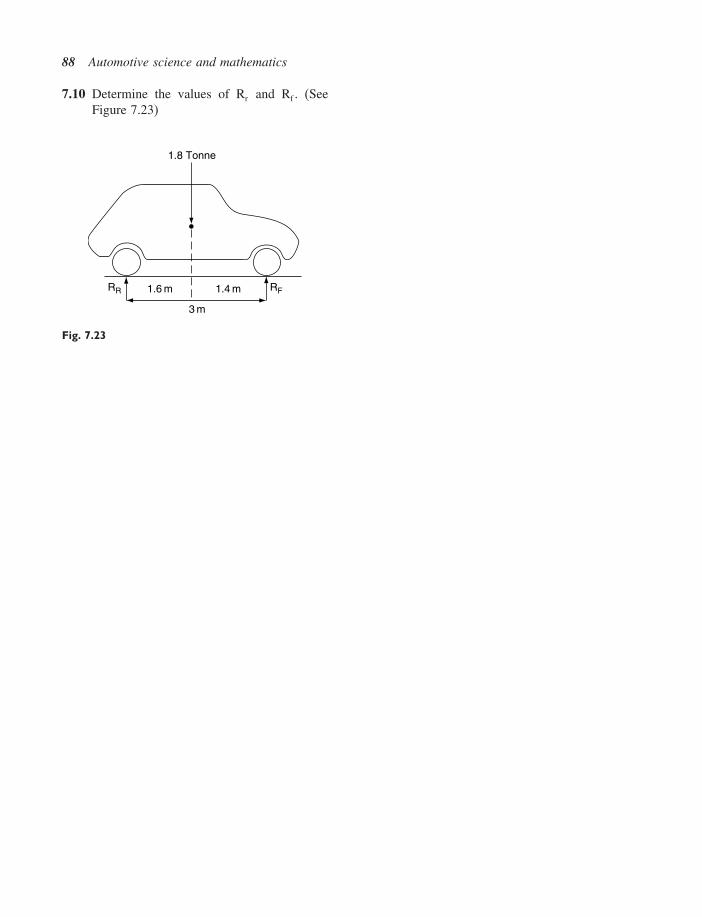
88 Automotive science and mathematics
7.10 Determine the values of Rr and Rf . (SeeFigure 7.23)
1.8 Tonne
1.4 m
3 m
1.6 mRR RF
Fig. 7.23

8Work energy, power and machines
8.1 Work
When an attempt is made to move a body, someresistance to movement occurs.
When lifting a body. as in Figure 8.1(a), theresistance arises from the force of gravity andwhen a body, such as the block shown inFigure 8.1(b), is moved along a horizontal surfacethe resistance to motion is caused by friction.
In both cases the force overcomes a resistanceand causes the body to move and work is done.
F = W × g Newtons
W
x m
x m
W × g Newtons
F
Friction Force
(a)
(b)
Work Done AgainstFriction = F × x J
Work Done Against Gravity =W × g × x N m = W × g × x Joule
Fig. 8.1 Work = force × distance
The work done is found by multiplying the forceby the distance moved.
Work done = force × distance moved in thedirection of action of the force.
The distance is measured in metres and the forcein newtons.
1 metre ×1 newton = 1 m N = joule (8.1)
Example 8.1A vehicle is towed along a level surface for adistance of 200 m, by a force of 8 kN. Calculatethe work done in moving the vehicle.
SolutionWork done = force ×distance moved
= 8000 N ×200 m
= 1 600 000 N m
= 1 600 000 J� because
1 N m = 1 joule
8.2 Power
Power is the rate of doing work, i.e. power
= work done in joulestime taken in seconds
Power is measured in watts:
Power P in watts = work done in joulestime taken in seconds
(8.2)

90 Automotive science and mathematics
Because the watt is a small unit of power, thepower of vehicle engines is normally quoted inkilowatts (kW).
Example 8.2A vehicle is pushed along for a distance of 200metres by a force of 220 newtons for a period of 10seconds. Calculate the power that this represents.
SolutionWork done = force ×distance
= 220 N ×200 m
= 44 000 J
= 44 kJ
Power P = Work done÷Time taken in seconds
P = 44 kJ ÷10 seconds
P = 4�4 kW
8.3 Work done by atorque
Figure 8.2 shows a force of F newtons acting ata radius of r metres. The force moves throughan arc from P to Q. The distance moved, d, isan arc whose length is r� metres, where r is theradius in metres and � is the angle in radians.The work done by F in moving from P to Q =force ×distance = F × r�. But F × r = torque T.
∴ Work done by a torque = T� (8.3)
In words, work done = torque × radians
dF
FP
Qrθ
D o R
Work Done = Force × Distance= F × r θ
T = F . rWork Done = T θ
Where θ = Angle in Radians
Fig. 8.2 Torque-work
Example 8.3A torque of 200 N m is applied to a shaft. Calculatethe total work done when the shaft rotates 1000times.
SolutionAs there are 2� radians in one revolution the workdone per revolution is = 2��T.
The work done in N revolutions = Work donein one revolution × N
Total work done = 2��T�N
= 2� ×200×1000
= 1 256 800 N m
= 1�2568 MJ
8.4 Work done by aconstantly varying force
Figure 8.3 shows a chain type block and tacklelifting gear. The weight being lifted is made upfrom the weight of chain plus the hook and theactual load. As the load is raised, the amount ofchain associated with the load decreases.
Example 8.4A chain-type lifting tackle is used to raise a loadof 75 kg through a height of 2.5 metres. At thestart of the lift the length of chain supporting theload is 12 m, and during the lift 5 m of chain arewound in. If the chain weighs 6 kg per metre andthe pulley weighs 4 kg, determine the work doneon the load in lifting it through the distance of2.5 m. Take g = 9�81 m/s2.
SolutionThe initial load
= Chain +pulley+ load
= �12×6×9�81�+ �4×9�81�+ �75×9�81�
= 1481 N

Work energy, power and machines 91
MORRIS
Fig. 8.3 Chain-type block and tackle lifting machine
The final load = �7×9�81+75×9�81�
= 804�4 N
The distance moved by the load = 2�5 m
The work diagram in Figure 8.4(a) shows theoperation.
The area under the work diagram = work done.
Work done = �1481+804�4�
22�5 J
= 2857 J
Distance = Metres2.5 m0
(a)
804.4 NForceNewtons
1481 N
Work Done =
= 2857 N m = 2857 J
1481 + 804.42
× 2
Area = Work Done
( )
Mid Ordinates
Width of Strip = 5 m
82 100 88 50 27 14
100
80
60
40
(b)
20
P N
ewto
ns
Mid Ordinate
5 10 15 20 25 30
Δ Metres
Fig. 8.4 Work diagram – variable force (Examples 8.4and 8.5)
Mid-ordinate method forcalculating work done
Example 8.5A body has a variable pull of P newtons acting onit. Values of P and the distance D from rest are asshown in Table 8.1.
Plot a graph of P against D and use it to deter-mine the amount of work done in moving the bodythrough the distance of 30 m.
Table 8.1 Plotting a graph of P and D to find workdone, using the mid-ordinate rule (Example 8.5)
D (m) 0 2 5 8 10 14 18 22 25 30P (N) 60 80 100 100 96 80 48 30 20 0

92 Automotive science and mathematics
SolutionPlot the graph as shown in Figure 8.4(b).
Mid ordinate ruleDivide the total base into a suitable number ofequal parts and erect ordinates at the mid point ofthe base of each strip. Each strip is then consideredto have an area equal to the width of one strip ×mid ordinate length. Because each strip has thesame width the total area is equal to the sum ofthe mid ordinates multiplied by the width of onestrip.
In Example 8.5 the mid ordinates are: 82, 100,88, 50, 27, 14
The width of each strip = 5 mThe area under the curve = 5�82+100+88
+50+27+14�
= 5×361 N m
= 1�805 kJ
Are under curve = work done = 1.805 kJ
8.5 Energy
Energy is the ability to do work. The unit of energyis the joule.
Potential energy is the energy that a body pos-sesses by virtue of its height above some datum.Water, held back by a dam, in the reservoir ofa hydro-electric power station whose turbines areat a lower level holds large reserves of potentialenergy.
Potential energyPotential energy is the type of mechanical energythat a body possesses by virtue of its position; atypical example is water held in a reservoir whichis used to drive water turbines for the generationof electricity. Another example is the energy thatis stored in a spring brake that is held there untilthe brake is applied.
Chemical energyThe energy that drives the engine is derived fromthe chemical energy that is stored in the fuel. Thechemical energy is converted into heat by the com-bustion process.
Conservation of energyThe principle of conservation of energy states thatenergy can neither be created nor destroyed. It canbe changed from one form to another; for example,chemical energy can be transformed into electricalenergy. This happens when energy is drawn from abattery to operate a starter motor; heat energy canbe transformed into mechanical energy as happenswhen fuel is burned in an engine to drive thepistons; and so on.
Energy equationSince energy is the capacity of a body to do workany change in the energy content of a body isaccounted for by either (a) work done on the bodyor (b) work done by the body. In the form of anequation this becomes:
Potential energy+kinetic energy+work done
= constant
Kinetic energyKinetic energy is the energy that an object pos-sesses by virtue of its velocity.
Consider the motion of a body of mass m kgthat is moved by a force of F newtons through adistance of l metres.
Work done on the body = F × l �i�
The acceleration produced, a�= F/m �ii�
At end of the distance l the velocity v ofthe body may be obtained from the equationv2 = u2 +2al�u = 0�∴ l = v2/2a

Work energy, power and machines 93
Substituting for a from Equation (2) gives
l = v2m2F
Work done = Fl = F�v2m2F
= mv2
2The work done on the body by the force F in
moving through the distance l is 1/2 mv2.By the principle of conservation of energy, the
work done is converted to converted to kineticenergy.
Kinetic energy is calculated by multiplying halfthe mass of the object by the square of the velocityof the object.
If the mass is m kg and the velocity is v m/s,the kinetic energy is calculated from the formula
k�e� = 1/2 mv2 (8.4)
Example 8.6A vehicle of mass = 1200 kg is travelling at20 m/s. Calculate the kinetic energy of the vehicle.
SolutionMass m = 1200 kg, velocity v = 20 m/sKinetic energy = half the mass×velocity squared
= 1200/2×20×20 J
= 600×400 J
= 240 000 J
Example 8.7A motor car with a mass of 1.2 tonnes is sloweddown from a speed of 72 km/h to 45 km/h byapplication of the brakes. Calculate the change ofkinetic energy that occurs during this process andstate what happens to this energy.
SolutionInitial velocity u = 72 × 1000/3600 = 20 m/s;final velocity v = 45 × 1000/3600 = 12�5 m/s.Mass m = 1200 kg.Change of kinetic energy = 1/2 −1200�202 −12�52�
= 600�400−156�25�
= 146�25 kJ
The kinetic energy is converted into heat throughfriction at the brakes and is then dissipated throughthe atmosphere.
Energy of a falling bodyConsider an object of mass m kilogram that is ona ledge at height h metres above the ground. Ifthe object is pushed off the ledge it will fall tothe ground and as it falls the potential energy isreduced because the height above the ground levelis reduced. However, the velocity of the objectincreases as falls and this results in an increase inkinetic energy.
As no external work is done by the object, thetotal energy which it possesses remains constant.
Potential energy + kinetic energy = constant
Total energy before falling = potential +kinetic
= mgh +0
= mgh joules
Since no work is done by the object while fallingh metres, the total energy on reaching the groundmust equal mgh joules. At the instant that theobject reaches the ground the only energy that itpossesses is kinetic.Total energy on reaching the ground
= potential + kinetic= 0+1/2 m v2
Because no work has been done,mgh = 1/2 m v2
which gives v = √2gh.
Kinetic energy of rotationWhen a body such as an engine flywheel is rotat-ing, the whole of the rotating, mass (weight) isconsidered to be concentrated at a certain radiusthat is known as the radius of gyration.
Consider a flywheel (see Figure 8.5) of mass mkg and radius of gyration K metres revolving atN rev/s.
The linear velocity v of the concentrated massat radius K is: v = 2�KN m/s

94 Automotive science and mathematics
K
Flywheel Mass m kgRadius of Gyration k mI = m k2 KE = ½ I W2
Fig. 8.5 Kinetic energy of flywheel
The kinetic energy = 1/2 m v2 = 1/2 m�2�KN�2
2�N = angular velocity �, and mK2 = I themoment of inertia of the flywheel.
This gives another expression for kinetic energyof a flywheel, or similar rotating disc, namely:
k.e. of flywheel = 1/ 2 I�2 (8.5)
Where I = moment of inertia and � = angularvelocity in radians per second.
Example 8.8An energy-saving railcar is fitted with a systemthat transfers braking energy into a rotating fly-wheel. When acceleration is required, the energyfrom the rotating flywheel is transferred to therailcar’s propulsion system. The flywheel of theenergy-saving system has a mass of 0.5 tonneand a radius of gyration of 0.36 m. Determine thekinetic energy of the flywheel when it is rotatingat 1200 rev/min.
Solution
Kinetic energy of flywheel = 1/2 I�2�
� = 2�N/60 = 125 rad/s
I = m K2
= 500�0�36×0�36�
= 65 kg m2
k�e� = 1/2 ×65×125×125
= 507�8 kJ
8.6 Machines
A machine is a device that receives energy in someavailable form and converts it to a useable form.For example, a person may wish to lift a weight of2 tonnes; this is not possible unaided but the useof a jack or a hoist permits the person to achievetheir objective. A lever such as a pry bar is anexample of a simple machine. A relatively smallmanual force can be converted into a large forcein order to lift or move an object.
Figure 8.6 shows a hydraulic trolley jack. Aload of 2 tonnes (196 kN) is being lifted by aneffort of 150 N. In order to perform this operationthe operator will make several pumps of the han-dle, which means that the effort will move muchfurther than the load.
Machines exist in many different forms but thefollowing rules apply to them all.
Mechanical advantageThe mechanical advantage of a machine is theratio of the load to the effort:
mechanical advantage MA = loadeffort
Lifting machines such as jacks and cranes havea large mechanical advantage so that relativelysmall manual forces can be used to raise heavyweights.
Load 2 Tonne
Effort = 250 N
Trolley Jack as a Machine
Fig. 8.6 Trolley jack (Example 8.9)

Work energy, power and machines 95
Velocity ratio (movementratio)The velocity ratio, VR, of a machine, or movementratio, MR, is the ratio of the distance moved bythe effort to the distance moved by the load:
movement ratio MR = distance moved by effortdistance moved by load
Efficiency of a machineThe efficiency of a machine = (energy output/energy input) in the same time and this also
= MAVR
×100%
Example 8.9In the trolley jack example shown in Figure 8.6an effort of 250 newtons is lifting a load of 2tonnes. In lifting the load through a distance of15 cm the operator performs 40 pumping strokesof the handle each of which is 50 cm long. Calcu-late the mechanical advantage, velocity ratio andefficiency of the jack.
Solution
MA = loadeffort
= 2×1000×9�81250
MA = 78�5
MR = distance moved by effortdistance moved by load
= 40×5015
= 133�3
The efficiency = energy outputenergy input
×100
= �MA/VR�×100
= �78�5/133�3�×100
= 59%
Work done against frictionIn the example of the jack, the energy input =effort×distance moved = 250×40×0�5 = 5000 J.In the same time, the energy output = load ×distance raised = 2000×9�81×0�15 = 2943 J.
The difference between the input energy of5000 J and the output energy of 2943 J is a lossof 2057 J. This loss of energy is accounted for bywork done against friction in the machine.
Example 8.10When using a simple floor crane, the operatorinputs 25 000 joules to lift a load of 1 tonnethrough a height of 1.2 metres. Taking g =9�81 m/s2 calculate the efficiency of the crane anddetermine the energy loss due to friction.
Solution
efficiency = energy outputenergy input
energy output = work done in lifting the load
= 1000×9�81×1�2
= 11 772 J
∴ efficiency = 11 77225 000
= 0�471
= 47�1%
energy loss due to friction = 25 000−11 772
= 13 228 J
A steering mechanism as amachineThe force required to steer a vehicle is oftenconsiderably larger than a driver can comfort-ably exert. The steering mechanism is a machinethat allows the driver of a vehicle to operate thesteering without having to exert a large force atthe steering wheel. The rack and pinion steering

96 Automotive science and mathematics
Pitch
Pinion
Rack
Steering Force S.
Steering WheelForce F.
Steering Wheel
R
r
Fig. 8.7 Rack and pinion as a machine
mechanism that is widely used on light vehiclesis a convenient example of such a machine (seeFigure 8.7).
The steering wheel radius = RThe tangential force at the rim of the steering
wheel = F (this is the effort)The number of teeth on the pinion = NtThe circular pitch of the pinion gear = pThe force produced at the rack = S (this is the
load)
The mechanical advantage MA = LoadEffort
= SF
Consider one revolution of the steering wheel.
The circular pitch of the gear is thedistance between the teeth as measured on thecircumference of the pitch circle – one revolutionof the pinion is a circular distance of Nt×p, whereNt = number of teeth on the pinion. This is thedistance that the rack moves when the steeringwheel makes one revolution.
The movement ratio MR = distance moved by effortdistance moved by load
= 2�RNt�p�
Example 8.11A rack and pinion steering system has 5 teethof 10 mm pitch and a steering wheel of 320 mmdiameter. Calculate:
(a) the movement ratio(b) the mechanical efficiency of the steering gear
if a tangential force of 30 N at the rim of thesteering wheel produces a force of 560 N onthe rack.
Solution
�a� MR = 2�R
= 2×� ×160Nt�p�
= 10 005�45×10
= 20�1
�b� Mech. effcy = MAMR
MA = loadeffort
= 56030
= 18�7
∴Mech. effcy = 18�720�1
= 0�93 = 93%

Work energy, power and machines 97
Example 8.12A worm and sector steering gear of the typeshown in Figure 8.8 has a 4-start worm and asector that is a sector of a 48-tooth worm wheel.The steering wheel has a diameter of 400 mmand the drop arm has a length of 150 mm. Twotangential forces each of 15 N applied at the rimof the steering wheel produce a force in the draglink of 450 N, which acts at right angles to thedrop arm. Calculate:
(a) the movement ratio, MR, of the steeringsystem;
(b) the mechanical advantage, MA, of the system;(c) the mechanical efficiency of the system.
Solution
(a) MR = distance moved by effortdistance moved by load
The worm is 4-start so the worm wheel(sector) rotates by four teeth when the steeringwheel makes one revolution.
The distance moved by effort at the steeringwheel during one revolution = 2� × 200= 400�
Distance moved by load = 448
× 2� × 150= 25�
∴MR = 400�
25�= 16
(b) MA = loadeffort
= drag link forcesteering wheel force = 450
30= 15
(c) Efficiency =MAMR
×100 = 1516
×100 = 94%
8.7 Summary of formulae
Work done = force × distance. Units are joulesEnergy is ability to do work, units are joulesWork done = area under force against distance
graph
Kinetic energy = mass×velocity2
2
Mechanical advantage (MA) = loadeffort
Movement ratio (MR)
= distance moved by effortdistance moved by load
Efficiency of machine = MA ×100MR
Efficiency = energy outputenergy input
k.e. of flywheel = 1/2I�2
Potential energy + kinetic energy + work done= constant
Work done by torque = T�, where T = torquein N m and � = angle in radians
Worm
Sector
Steering Gear
(a)
15 N
15 N
Steering Wheel Dia = 400 mmDrop Arm Radius = 150 mm
R = 200 m
r = 150 mm
450 N
Drop Arm
4 Start Worm
(b)
Fig. 8.8 Worm and sector steering gear (Example 8.12)

98 Automotive science and mathematics
8.8 Exercises
8.1 In climbing an incline 200 metres long atruck exerts a steady pull of 1 kN on a trailer.Calculate the total work done by the truck.
8.2 During the power stroke of a certain dieselengine that has a stroke of 160 mm, theforce acting on the piston varies throughoutthe length of the power stroke as shown inTable 8.2; F = force on piston, D = dis-tance the piston moves from TDC. Use themid-ordinate rule to calculate the work donein kilojoules during this process.
Table 8.2 Calculation using mid-ordinate rule(Exercise 8.2)
F (kN) 75 80 70 60 55 43 28 18 5D (mm) 0 20 40 60 80 100 120 140 160
8.3 An engine develops a torque of 400 N m at acrankshaft speed of 1200 rev/min. Calculate:(a) the work done per revolution;(b) the power in kW.
8.4 An vehicle engine develops a torque of180 N m at a speed of 3000 rev/min.Calculate:(a) the engine power at this speed;(b) the torque at the gearbox output shaft
when the vehicle is in third gear, whichis 1.2:1, and the gearbox efficiencyis 96%.
8.5 The wheel, tyre and hub assembly for a cer-tain truck has a combined weight of 200 kg.If the radius of gyration of the assembly0.15 m, calculate:(a) the kinetic energy of the assembly when
it is rotating at 5 rev/s;(b) the work done by, and the power of,
the brake when the wheel is brought torest from this speed in a period of 1.5seconds.
8.6 A certain rear axle final drive has gearratio of 6:1. At a propeller shaft speed of
1800 rev/min the input torque to the finaldrive is 420 N m. Calculate:(a) the speed of the crown wheel in rev/min;(b) the torque at the crown wheel when the
final drive efficiency is 95%.8.7 An articulated vehicle of 40 tonnes gross
weight and travelling at 72 km/h is broughtto a standstill by the brakes in a distance of180 m. Calculate the average braking force.
8.8 A hydraulic system on a tipper truck liftsa load of 2 tonnes through a distance of0.125 m while the effort moves through adistance of 20 m. Calculate:(a) the movement ratio;(b) the actual effort required if the effi-
ciency of the lifting system is 75%. Takeg = 10 m/s2.
8.9 An effort of 180 N will lift a load of 3860 Nin a certain lifting machine. If the efficiencyof the machine is 80% what is its movementratio?
8.10 In a test on a hoisting machine it is found thatthe effort moves 0.6 m while the load risesby 40 mm. Find the effort required to lift aload of 1 tonne assuming an ideal frictionlessmachine. Take g = 10 m/s2
8.11 A trolley jack requires an effort of 200 new-tons to lift a load of 2 tonnes. In liftingthe load through a distance of 15 cm theoperator performs 40 pumping strokes ofthe handle each of which is 50 cm long.Calculate the mechanical advantage, move-ment ratio and efficiency of the jack. Takeg = 10 m/s2.
8.12 A vehicle is towed along a level surface fora distance of 400 m, by a force of 8 kN. Cal-culate the work done in moving the vehicle.
8.13 A vehicle is pushed along at uniform speedfor a distance of 200 metres by a force of120 newtons for a period of 10 seconds.Calculate the power that this represents.
8.14 A vehicle hoist raises a vehicle weighing 1.8tonnes through a distance of 2 metres in 15seconds. If the overall efficiencyof the hoistis 80%, calculate the power of the lift motor.Take g = 10 m/s2.

9Friction
9.1 Introduction
Surfaces which appear to be quite smooth are,when minutely examined, normally found to havesurface irregularities and imperfections. When twosuch surfaces are made to slide, one over theother, these surface imperfections cause resistanceto motion. This resistance to motion is calledfriction.
In Figure 9.1(a) the surface imperfections areenlarged. The peaks of the imperfections slot intovalleys and as one surface moves over the otherthe force causing movement attempts to break thepeaks off; this causes the resistance to movementthat is known as friction and also results in wearand deposition of particles in surrounding partsof any mechanism. Figure 9.1(b) shows the samesurfaces separated by a layer of oil. The layer ofoil separates the surfaces so the one may slide overthe other with reduced resistance to movement;lubrication also reduces wear.
A
B
(a) xxx Surfaces (b) Oil between Surfaces
A
B
Fig. 9.1 Friction
Coefficient of frictionThe apparatus shown in Figure 9.2 is used todetermine the coefficient of friction. The blockW is loaded with suitable weights. Other weightsare then placed in the small weight pan and theamount is increased until W moves steadily acrossthe flat surface on which it is placed. The weightof W (in newtons) represents the force pressingthe block on to the flat surface and the weight inthe pan represents the force F (in newtons) that
W
F
μ = FW
Fig. 9.2 Friction experiment

100 Automotive science and mathematics
causes the block W to move steadily along theflat surface.
The ratio of F to W is called the coefficient offriction and it is denoted by the symbol �.
Coefficient of friction � = FW
(9.1)
where F is the force to move the block and W isthe force pressing the surfaces together.
Example 9.1In an experiment to determine the coefficient offriction between brake lining material and steel,a force of 60 newtons steadily moves a blocklined with the brake lining material across a steelsurface. The block weighs 100 newtons. Calculatethe coefficient of friction.
� = F/W F = 60 newtons W = 100 newtons
� = 60/100
� = 0�6
Values of � for some materials are shown inTable 9.1.
Table 9.1 Some approximate values of �
Phosphor bronze on steel – dry 0.35Phosphor bronze on steel – oiled 0.15Steel on steel – dry 0.55Steel on steel – oiled 0.1Unworn tyre on dry tarmac 0.8Unworn tyre on wet tarmac 0.7 (falls rapidly as
speed increases)Brake lining material on steel 0.3
Static frictionThe force required to cause initial movementagainst friction is greater than the force requiredto maintain uniform motion.
Sliding frictionThe sliding force of friction is directly pro-portional to the force pressing the surfacestogether – this force is slightly less than the staticfriction force.
9.2 Making use of friction
ClutchTorque transmitted by a plate clutchIn the single plate clutch shown in Figure 9.3 theforce provided by the springs is applied uniformlyover both sides of the friction surfaces of theclutch plate. The friction force �F� = �W, whereW = total spring force.
This force acts at the mean radius of theclutch linings = R1 + R2/2, where R1 and R2
are the inner and outer radii of the clutch lin-ings respectively. The maximum torque that theclutch can transmit = friction force×mean radiusof clutch linings.
∴ Clutch torque T=�W · R1 +R2
2, but this is
for one side of the clutch lining.
R2 R12
Mean Radius ofLinings = R1 + R2
Fig. 9.3 Single plate clutch

Friction 101
There are two sides to the clutch plate so themaximum torque is
T = 2(
�W · R1 +R2
2
)
In general the formula for torque transmitted by aplate clutch is
T = n ·�W ½ �R1 +R2� N m (9.2)
where n = number of friction surfaces.
Example 9.2Figure 9.4 shows a twin plate clutch. The lin-ings have an inner radius of 250 mm and an outerradius of 320 mm. The total spring force is 4 kNand the coefficient of friction of the linings andthe pressure plate and flywheel is 0.35. Calcu-late the maximum torque that this clutch cantransmit.
4 Friction Surfaces
Fig. 9.4 Twin plate clutch (Example 9.2)
SolutionT = n · � W 1/2 �R1 +R2�Mean radius of linings= ½ �0�25 = 0�32� =0�285 mNumber of friction surfaces n = 4T = 4×0�35×4000×0�285T = 1596 N mT = 1�6 kNm
Power transmitted by a clutch
Power = �2 � T N�
1000kW, where T is torque in N m,
N = revolutions per second.
Example 9.3Calculate the maximum power transmitted by asingle plate clutch at speed of 3600 rev/min if thecoefficient of friction is 0.4 and the linings havea radii of 160 mm inner and 190 mm outer. Thetotal spring force is 2.5 kN.
SolutionMaximum clutch torque = �W n 1/2 �R1 +R2�Rev/min = 3600; ∴ rev/sec = 3600/60 = 60Mean radius = 1/2 �0�16+0�19� = 0�175 mW = 2500 NT = 0�4×2500×2×0�175 N m = 350 N m
Power = �2� T N�/1000
= �2×3�142×350×60�/1000
Power = 132 kW
Belt driveBelt drive systems rely on friction between the beltand the pulley for their ability to transmit power(Figure 9.5). The friction force derives from theforce exerted on the pulleys by the difference intension between the tight and slack sides of thebelt, T1 −T2. In a V-belt drive the friction force isprovided by the sloping sides of the pulley groovesand this serves to increase the effectiveness ofthese drives.

102 Automotive science and mathematics
ForceForce
Vee Belt(b)
Pulley
Belt
Belt Drive
(a)
Tight Side
Slack Side
T1
T2
Fig. 9.5 Belt drive
Torque transmitted by belt driveIn both cases the effective torque is T = �T1 −T2� r,where T is the torque in N m, T1 and T2 are thebelt tensions in newtons, and r = radius of pulleyin metres.
Power of belt drivePower = �2� T N�/1000
Power = 2��T1 −T2� r N1000
kW� where N = rev/s
(9.3)
Example 9.4A pulley of a certain belt drive system has a diam-eter of 45 mm and it rotates at 1800 rev/min. If thebelt tension is 180 N on the tight side and 45 N onthe slack side, calculate the power that is beingtransmitted by the belt drive.
SolutionPower = �2 � T N�/1000
= �2 � �T1 −T2� r N/1000�
where N = rev/s
�T1 −T2� = �180−45� = 135 N
r = 0�045/2m� N = 1800/60 = 30
Power = �2 � ×135×0�0225×30�/1000
= 0�573 kW
Speed ratio of belt driveIn the belt drive shown in Figure 9.6 the smalldiameter wheel is driving the larger one. One revo-lution of the small wheel produces �×15 = 47�12millimetres of movement of the belt.
This produces the same amount of movementaround the circumference of the large wheel.
The circumference of the large wheel = � ×30 = 94�24 mm.
A movement of 47.12 mm on the circumferenceof the large wheel represents an angular movementof �47�12/94�24�×360� = 180� = 1/2 revolution.
In general, speed ratio of belt drive system
= Nl/Ns
= Ds/Dl (9.4)
Where Nl = rev/min of large wheel, Ns = rev/minof small wheel , Ds = diameter of small wheel andDl = diameter of the large wheel.
Speed Ratio = 2.130 mm15 mm
Fig. 9.6 Speed ratio – belt drive

Friction 103
9.3 Brakes
Drum brake – basic principleFigure 9.7 shows the basic principle of a drumbrake with one leading shoe and one trailing shoe.
The actuating force P is provided by a hydrauliccylinder or cam. The shoes are pivoted at A1
and A2.The action of force P creates a friction force
between the rotating brake drum and the brakelining.
The friction force on the leading shoe is �F andit acts tangentially to the drum. On the trailingshoe the friction force is �F1.
The pivots are distance y from the centre of thedrum and the actuator force P is at distance Xfrom the pivots. The drum radius is R.
Action of the leading shoeTaking moments about pivot A1, Px = Fy−�FR
F = P x/�y−�R� (9.5)
Action of the trailing shoeTaking moments about pivot A2, Px = F1y+�F1R
F1 = Px/�y+�R� (9.6)
The effective braking force on the leading shoe isgreater than that on the trailing shoe. It should benoted that this effect is dependent on the directionof rotation of the brake drum, which is the reasonwhy two leading shoe brakes are less effectivewhen reversing a vehicle.
Example 9.5In a certain drum brake the distance x as shown inFigure 9.7(b) is 12 cm, the distance y is 24 cm andthe drum radius R = 14 cm. If the actuating forceP is 800 newtons and the coefficient of friction� = 0�4 calculate the effective friction forces oneach of the brake shoes.
SolutionNormal force on leading shoe
F = Px
�y−� R�
= 800×12�24−0�4×14�
F = 9600�24−5�6�
F = 522 N
Normal force on trailing shoe
F1 = Px
�y+� R�
F1 = 9600/�24+5�6�
F1 = 324 N
Disc brakeThe disc brake shown in Figure 9.8 utilisesopposed cylinders to apply force to the frictionpads and these pads apply a clamping force to thedisc. In Figure 9.8 the following data apply:
hydraulic pressure is P N/m2; area ofthe pistons is A m2; the coefficient offriction between the pads and the disc is�; the effective radius of the brake isR m. The hydraulic force on each pad =P × A newtons.
The friction force at each pad = �PA newtons
The braking torque
= 2R�PA newton metres (two pads) (9.7)
Example 9.6In a disc brake of the type shown in Figure 9.8 thehydraulic pistons are 50 mm in diameter and theeffective radius of the brake disc is 150 mm. Cal-culate the braking torque when the hydraulic pres-sure is 20 bar and the coefficient of friction is 0.4.

104 Automotive science and mathematics
Trailing Shoe
Leading Shoe
(a)
DoR
μF and μF1 = Friction ForcesDrum Radius = R Actuating Force = PF and F1 = Normal Force Created by P
Action of Leading ShoeTaking Moments about Pivot A1 Px = F y – μF R
F = Px
(y – μR)
Action of Trailing Shoe
Taking Moments about Pivot A2 Px = F1 y + μF1 R
∴ F1 = Px
(y + μR)
The Force F at the Leading Shoe is Greater than F1 At the Trailing Shoe.(b)
P
R
F
Drum RotationBrake Actuating Force
μF1
μF
F1
yx
ab
O O
BrakeDrum
A1 A2
Fig. 9.7 Drum brake

Friction 105
HydraulicPressure
Caliper
Disk Brake
Disc
Brake Pad
R = Effective Radius.
Piston Area = A Hydraulic Pressure P Force on Pad F = P × AFriction Force at Each Pad = μPA There are 2 PadsTotal Friction Force = 2 μPA Braking Torque = 2 μPA × R
Fig. 9.8 Disc brake
SolutionBraking torque = 2R�PAP = 20×100 000P = 2 000 000 NA = � d2/4A = 1�96×10−3 m2
R = 0�15 mBraking torque = 2 × 0�15 × 0�4 × 2 000 000 ×�1�96/1000� = 470 N m.
TyresTyres rely on friction between the tyre tread andthe driving surface to provide the grip for drivingpurposes. The coefficient of friction for tyres isaffected by the rubber compounds used in the tyreconstruction, the tread pattern, the tyre dimensions(low profile) the type and condition of the drivingsurface and the speed of the vehicle etc. The graphin Figure 9.9 gives an indication of tyre frictionon different surfaces.
Anti-lock braking systems (ABS) make use ofthe fact that greater friction is obtained when the
1.0
0.8
0.6
0.4
0.2
20 40 60 80 100
Dry Tarmac
Wet Tarmac
Loose Gravel
Non Comacted Show
Slip %Approximate Type Friction
Friction
Coe
ffici
ent o
f Fric
tion
μ
Fig. 9.9 Tyre friction
amount of slip is kept at a low level. Tractioncontrol systems are also designed to control slipand thus maximise tyre friction.

106 Automotive science and mathematics
Braking efficiencyThe power of a braking system is determined ulti-mately by the friction between the tyres and thedriving surface. The concept of braking efficiencyis based on the assumption that the coefficient offriction between tyre and driving surface can neverbe greater than 1. Figure 9.10 shows a vehiclewith its wheels locked by the brakes being pulledalong horizontally by a force that is equal to theweight of the vehicle. The retardation achievedunder such conditions is equal to gravitationalacceleration g �9�81 m/s2� and this is taken to be100% braking efficiency. If the actual retardationof a vehicle under braking is a m/s2 the brakingefficiency is a/g×100%.
Braking efficiency = �a/g�×100% (9.8)
F = ma
W = mgWheels Locked by Brakes
∴ a/g = 1 or a = g For 100% Braking
μ = FW
mamg
= = 1
Fig. 9.10 Braking efficiency
Example 9.7The maximum braking deceleration of a certainvehicle is 7�2 m/s2. Calculate the braking effi-ciency. Take g = 9�81 m/s2.
SolutionBraking efficiency = �a/g�×100%Braking efficiency = �7�2/9�81�×100Braking efficiency = 73%
Static brake testsIn the UK, brake efficiency tests are performedon machines that measure the horizontal brakingforces at each wheel. These forces are then addedtogether to give a total horizontal braking force forthe vehicle; this total force is then divided by the
weight of the vehicle to give the braking efficiencyof the vehicle under test station conditions.
Figure 9.11 shows the basic principle of adynamometer that is used to determine brakingforces on a vehicle. The vehicle is driven on to therollers, one for each side of the axle, and the frontand rear axles are tested separately. An electricmotor drives the test rollers. The rollers are drivenby the armature shaft and the casing of the electricmotor is free to rotate on its axis but is restrainedfrom doing so by a torque arm and spring balance.The torque exerted by the motor and roller on thewheel and tyre is equal and opposite to the torquemeasured at the torque arm of the electric motor.
In the diagram, FB = braking force, r = radiusof roller, F = force on torque arm of the electricmotor, and R = radius of torque arm.
Torque at point of contact between tyre androller = torque at the electric motor:
∴ FB · r = F · R
FB = FR/r
In practice, the force at the torque arm is measuredby a transducer and the reading is transmitted togauges on a console and the braking forces for theleft-hand and right-hand side of the vehicle can becompared. The total braking force (front + rear)is divided by the weight of the vehicle to give thebraking efficiency.
This test relies on the following principles ofmechanics.
Retarding force F = M·a,
where F = braking force,
M = mass of vehicle and
a = retardation of vehicle.
F = M�a
∴ a = F/m
Braking efficiency = �a/g�×100%
Substituting for F/m for a in this equation gives
braking efficiency = F ·100Mg
(9.9)

Friction 107
Braking Force FB
Radius of Roller = rTorque Reaction Arm Radius = RTorque Arm Force = F
FB × r = F × R ∴ FB = F × R
r
M F
FB
R
r
Braked Wheel
Roller-Type Brake Tester Measuringthe Braking Force at each Wheel
Roller
Fig. 9.11 A static brake test
Where Mg = weight of vehicle in newtons∴ braking efficiency = �F/M�×100, where M =weight of vehicle in kg×9�81 and F = total brak-ing force in newtons.
Example 9.8In a test-station brake-test on a vehicle, the frontbrake forces total 2200 N and the rear brake forcestotal 1400 N. If the vehicle has a mass (weight) of1.2 tonne, calculate the braking efficiency. Takeg = 9�81 m/s2.
SolutionBraking efficiency BE = (total braking force ÷weight of vehicle in newtons)×100BE = �3600/1200×9�81�×100BE = �3600/11772�×100BE = 31%
9.4 Angle of friction
If a block of weight W is placed on an adjustableinclined plane such that the angle of the inclinecan be altered from zero degrees to the angle atwhich the block will slide at uniform velocitydown the slope, the forces acting are as shownin Figure 9.12. The angle at which this occurs isknown as the angle of friction.The forces acting are
force acting down the slope = W sin
force pressing block on to slope = W cos
the coefficient of friction �
= force pressing surfaces togetherforce moving the block
∴ � = Wsin
Wcos= tan (9.10)
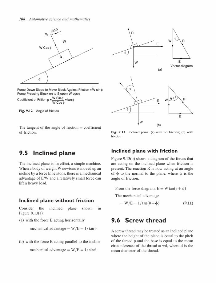
108 Automotive science and mathematics
W Cos φ
Force Down Slope to Move Block Against Friction = W sin φForce Pressing Block on to Slope = W cos φ
Coefficient of Frition μ =
W Sin φ = tan
φ
W
W
φ
Sin φ
W Cos φ
Fig. 9.12 Angle of friction
The tangent of the angle of friction = coefficientof friction.
9.5 Inclined plane
The inclined plane is, in effect, a simple machine.When a body of weight W newtons is moved up anincline by a force E newtons, there is a mechanicaladvantage of E/W and a relatively small force canlift a heavy load.
Inclined plane without frictionConsider the inclined plane shown inFigure 9.13(a).
(a) with the force E acting horizontally
mechanical advantage = W/E = 1/ tan �
(b) with the force E acting parallel to the incline
mechanical advantage = W/E = 1/ sin �
W
E
(a)
R
θ
W
EVector diagram
Rθ
E
(b)
E
R
W
W
θ
θ + φ
φ
Fig. 9.13 Inclined plane: (a) with no friction; (b) withfriction
Inclined plane with frictionFigure 9.13(b) shows a diagram of the forces thatare acting on the inclined plane when friction ispresent. The reaction R is now acting at an angleof to the normal to the plane, where is theangle of friction.
From the force diagram, E = W tan��+�
The mechanical advantage
= W/E = 1/ tan��+� (9.11)
9.6 Screw thread
A screw thread may be treated as an inclined planewhere the height of the plane is equal to the pitchof the thread p and the base is equal to the meancircumference of the thread = �d, where d is themean diameter of the thread.

Friction 109
d
p
RW
E
Screw Thread
Π d
p
Force Diagram
R
E
Wφ
θ
θ + φ
Fig. 9.14 Screw thread as inclined plane
The forces acting on screw thread are the sameas those on the inclined plane with friction. Thevector diagram for the forces acting on the threadare shown in Figure 9.14(b). The horizontal forceE = W tan��+�, where � = helix angle of threadand is the angle of friction.
The torque required to tighten the nut againstthe axial force W = d/2�E
Torque = Wd2
tan ��+� (9.12)
because E = W tan ��+�
V-threadFor a V-thread the normal force R between thenut and the thread is increased since the verticalcomponent of R must be equal to W.
From the force diagram in Figure 9.15,R = W/cos�.
RW
2α
∴ R = W/Cos αFrictional Resistance = μ R =
= μ′ Wμ′ = Virtual Coefficient of Friction μ Cos α
WR
= Cos α
=
α
Cos αμw
Fig. 9.15 V-thread
∴ frictional resistance = �R
= �W/ cos �
= �′W
Where �′ = �/ cos �� is half the thread angle.The V-thread is therefore equivalent to a square
thread with a coefficient of friction �′ instead of �.
The angle of friction that corresponds to
�′ is ′ = tan−1 �′� (9.13)

110 Automotive science and mathematics
Example 9.9A screw jack has a thread of 45 mm mean diameterand a pitch of 7 mm. The thread is of V-formwith an included angle of 60� and a coefficient offriction � = 0�15. Calculate the torque required toraise a load of 1 tonne. Take g = 9�81 m/s2.
SolutionThe formula required here is the same as that forthe square thread except that the angle of frictionis ′ instead of .
Torque = Wd2
tan ��+��
because E = W tan ��+�
�′ = �/ cos � = 0�15/ cos 30�
= 0�15/0�8660 = 0�173
′ = tan−1 0�173 = 9�82�
tan � = pitch/mean circumference.
Mean circumference = 0�045 � = 0�143 m
Pitch = 0�007 m
tan � = 0�007/0�143 = 0�05
∴ angle � = 2�9�
∴ Torque = 1000×9�81×0�045/2
× tan�2�9� +9�82��
= 221× tan 12�72�
= 221×0�225
= 50 N m
9.7 Friction in a journalbearing
Figure 9.16 represents a shaft rotating inside aplain bearing. The radius of the shaft is r and theload acting is W. If the coefficient of a friction is�, the frictional force opposing motion is �W andthe resulting torque T = �Wr.
Torque T = μWr
F = μW
W
r
Fig. 9.16 Friction in a journal bearing
power lost in friction = 2� T N1000
kW�
Where N = shaft speed in rev/s�
∴ power lost in friction = 2�� W r1000
kW (9.14)
Example 9.10A 75 mm crankshaft main bearing journal rotatesat 3000 rev/min while carrying a normal loadW = 20 kN. If the coefficient of friction in thebearing = 0�02, calculate:
(a) the friction torque on the crankshaft;(b) the power lost in friction at this engine speed;
and(c) state what happens to the energy absorbed in
friction.
Solution(a) Friction force = �W = 0�02×20 000 = 400 N
Friction torque T = �W r = 400 × 0�0752
=15 N m
(b) Friction power
= 2� T N1000
kW� where N = shaft speed in rev/s
= 2� ×15×3000/601000
kW
= 4�71 kW
(c) The 4.71 kJ of heat energy is transferred to thelubricating oil and surroundings.

Friction 111
9.8 Summary offormulae
Laws of static friction1. Friction always opposes motion.2. The force of friction depends on the materials
and the properties of the surfaces in contact.3. When motion is about to take place, the
magnitude of the limiting friction is directlyproportional to force pressing the surfacestogether, that is:
Force of friction = coefficient of friction
× force pressing surfaces together
4. Friction is independent of surface area.
Coefficient of friction
� = friction forceforce pressing surfaces together
Friction torque = friction force
× radius at which it acts
9.9 Exercises
9.1 A metal casting weighing 250 kg is draggedalong a concrete floor surface by a force of1.2 kN. Determine the coefficient of frictionbetween the casting and the concrete floorsurface. Take g = 10 m/s2
9.2 A shaft of 50 mm diameter runs in a plainbearing while carrying a normal load of500 N. The coefficient of friction betweenthe bearing and the shaft is 0.08. Calculatethe friction torque.
9.3 What effect does lubrication have on thefriction of dry surfaces? Describe the prin-ciples of lubrication and explain the advan-tages of pressure lubrication for bearings.
9.4 A vehicle of mass 1.4 tonnes is pulled acrossa horizontal surface with the wheels locked,by a horizontal force 8 kN. Determine the
coefficient of friction between the tyres andthe surface. Take g = 10 m/s2.
9.5 Figure 9.17 shows a V-belt drive system ofthe type that is used in some Volvo vehicles.The effective diameter of the small pulleyis changed during operation by a centrifu-gal device and this provides a continuouslyvariable speed ratio. At a certain speed thesmall pulley has a radius of 60 mm. If thepower transmitted is 45 kW at a pulley speedof 3000 rev/min, calculate the difference intension between the tight and slack sides ofthe drive belt.
Driver
Driven
Variable Diameter
Centrifugal Device
Fig. 9.17 Belt drive variable ratio
9.6 The wheel-fixing studs on a certain truckhave a mean thread diameter of 20 mm andthe pitch of the thread is 2 mm. Determinethe torque required to produce a clampingforce W of 2.6 kN when the coefficient offriction �′ is 0.18.
9.7 The recommended tightening torque for ahub nut on a front wheel drive axle shaft

112 Automotive science and mathematics
is 205 N m with a lightly oiled thread. Thethread has a mean diameter of 24 mm, a pitchof 2 mm and a thread angle of 60�. Whenoiled as specified the thread has a coefficientof friction of 0.1, but when the thread is drythe coefficient of friction is 0.15. Calculate:(a) the axial force produced when the thread
is oiled;(b) the axial force produced when the thread
is dry; and(c) state the effect that the reduced axial
force will have on wheel-bearing pre-load and wheel security.
9.8 A certain twin plate clutch has a mean diam-eter of 0.20 m. If the coefficient of frictionof the linings and pressure plate/flywheelis 0.4, determine the minimum spring forcethat will be required to transmit 150 kW atan engine speed of 3000 rev/min.
9.9 If the coefficient of friction in a 75 mm diam-eter main bearing is 0.035, determine thepower absorbed in friction when the load onthe shaft is 500 N and the engine speed is1800 rev/min.
9.10 A disc brake has two opposing pads thatare operated by hydraulic pistons whichare 50 mm in diameter. If � = 0�4 and thepads act at an effective radius of 0.140 m,calculate:(a) the brake torque when the hydraulic
pressure applied to the pistons is 20 bar;(b) the braking force between the tyre and
the road if the wheel and tyre diameteris 0.65 m.
9.11 During a static brake test the following brak-ing force readings are obtained:
off-side front 2.1 kNnear-side front 2.05 kNoff-side rear 1.4 kNnear-side rear 1.38 kN.
(a) If the weight of the vehicle is 1.2 tonne,calculate the braking efficiency; takeg = 9�81m/s2;
(b) Check the MOT testers manual to estab-lish whether or not the side-to-sideimbalance shown is acceptable.

10Velocity and acceleration, speed
10.1 Speed and velocity
Speed is the rate at which distance is covered andspeed can be specified by its size alone. Velocityis a more specific quantity because it possessesdirection as well as size; velocity is said to be avector quantity.
velocity = distance coveredtime taken
10.2 Acceleration
Acceleration occurs whenever the velocity of anobject changes. When the velocity of an objectdecreases it is said to have decelerated.
acceleration = change in velocitytime taken
10.3 Velocity–time graph
Uniform velocityWhen an object travels at constant velocity ofv m/s for a given period of time, t seconds, a graphof velocity against time produces a straight line,as shown in Figure 10.1.
The area enclosed by this graph is v × t. As vis in metres/second and t is in seconds, the unitsof area cancel down to give metres.
Area = v × t
v
O
Vel
ocity
m/s
tTime – SecondsConstant Velocity
Area = vt metres
Area Undergraph = Distance Covered
Fig. 10.1 Constant velocity
This leads to the useful fact that the areaenclosed by a velocity–time graph is equal to thedistance covered.
distance = uniform velocity× time in seconds
Uniform accelerationWhen an object is accelerated uniformly from aninitial velocity of u m/s to a final velocity of v m/sthe graph produced is a straight line of the typeshown in Figure 10.2.

114 Automotive science and mathematics
uArea =
u + v2
tDistance S =
u + v
2 t
tTime
Vel
ocity
v
Fig. 10.2 Constant acceleration
The area enclosed by this graph is�u+ v�
2· t
Butu+ v
2is the average velocity
The distance covered = average velocity×time in seconds.
These basic principles of velocity and accelerationare used to develop a set of formulae that areknown as equations of motion.
10.4 Equations of motionand their application tovehicle technology
v = u+at
s = �u+ v�t
2
v2 = u2+2as
s = ut+at2
2
In these equations: u = initial velocity in m/s; v =final velocity in m/s; a = acceleration in m/s2;t = time in seconds; s = distance.
To convert km/h to m/s: multiply by 1000 anddivide by 3600.
Example 10.1A vehicle travels at a constant speed of 50 km/h for3 minutes; it then accelerates uniformly to a speed
20
40
60
80
km/h
1 2 3 4 5
60
Time Minutes
Distance Covered = Area under Graph
=
= 2.5 + 2.17 km = 4.67 km
× 50 + 50 + 80
2(360
× 2)
Fig. 10.3 Example 10.1
of 80 km/h in a period of 2 minutes. Draw a speedagainst time graph and determine the distance cov-ered by the vehicle in the 5-minute period.
Solution (Figure 10.3)Distance covered in first 3 minutes = 3/60 ×50 km = 2�5 kmDistance covered in next 2 minutes = 50+80
2·
2/60 = 2�17 kmTotal distance in 5 minutes = 4�67 km
Example 10.2A vehicle travelling at 72 km/h is braked uni-formly to a speed of 28 km/h in a time of 10seconds. Draw a speed–time graph and determinethe distance that the vehicle travels while it isslowing down.
Solution (Figure 10.4)Distance covered while slowing down = areaunder speed–time graph
Distance covered = 72+282
· 10003600
×10 = 139 m
Example 10.3A vehicle travelling at 60 km/h is braked to astandstill by a retardation of 24 m/s2. Use the

Velocity and acceleration, speed 115
Time Seconds
Spe
ed k
m/p
h
72 km/ph
28 km/ph
2 4 6 8 10
Distance Covered = Area under Graph
=
= 0.138 km = 138 m
72 + 282
× 10003600
× 10( )
Fig. 10.4 Example 10.2
equation v = u+at to determine the time takento stop the vehicle.
Solutionu = 60×1000/3600 = 16�7 m/sa = −24 m/s2
Final velocity v = 0v = u+at
∴ t = �v−u�
a
t = 0−16�7−24
t = 0�7 s
10.5 Force, mass andacceleration
Newton’s laws of motionThe basic laws used in the study of motion arethose that were first formulated by Sir Isaac New-ton in the seventeenth century. These laws are asfollows.
The law of inertia states that a body will remainin a state of rest or uniform motion in a straight
line until it is compelled to change that state bybeing acted upon by an external force.
The law of change of momentum states that therate of change of momentum is equal to theapplied force.
The law of reaction states that every action hasan equal and opposite reaction.
The basic unit of force is the newton; 1 newtonis the magnitude of the force that will producean acceleration of 1 m/s2 when applied to a massof 1 kg.
The relationship between force, mass and accel-eration is given in the following equation.
F = ma
where F = force in newtons, m = mass in kg,a = acceleration in m/s2.
10.6 Relation betweenmass and weight
The weight of an object is the amount of forcethat is exerted on the object by the gravity of theearth. If an object falls freely it will accelerateat the gravitational acceleration of 9.81 m/s2. Thegravitational acceleration is known as g.
The weight of an object = mass in kilograms ×gravitational constant.
This is normally written as weight = m × g,or mg.
In simple calculations the approximation of g =10 m/s2 is sometimes used.
10.7 Inertia
Inertia is the sluggishness or resistance that a bodyoffers to starting from rest or to a change ofvelocity.
Example 10.4A motorcycle and its rider increase speed from30 km/h to 80 km/h in a time of 5 seconds.

116 Automotive science and mathematics
Calculate the acceleration in m/s2. If the riderweighs 52 kg what force will be felt by the rider’sbody?
SolutionInitial velocity u = 30×1000/3600 = 8�33 m/sFinal velocity v = 80×1000/3600 = 22�22 m/st = 5 secondsv = u+at
∴ a = v−u
t= �22�22−8�33�
5= 13�89/5 = 2�78 m/s2
Force felt by rider = m×a= 52×2�78= 144�6 N
10.8 Motion undergravity
When a body is acted on by the attractive force ofthe earth and drawn towards the earth’s centre thebody is said to be moving under gravity. It can beshown that all bodies that are small in comparisonwith the earth, whatever their mass, are influencedin practically the same manner by this force ofgravity. The acceleration that is caused by theforce of gravity varies slightly across the earth’ssurface. A figure for gravitational acceleration thatis used as an average is g = 9�8 m/s2 and this isknown as the gravitational constant.
Example 10.5A vehicle falls off the edge of a viaduct 50 m high.How long will it take to reach the ground?
SolutionThe initial velocity u= 0 m/sThe acceleration a = g = 9�81 m/s2
The distance s = 50 metresUsing the equation s = ut + at2
2
50 = 0× t + 9�81 t2
2
100 = 9�81 t2
t = √�100/9�81�
t = 3�2 secondsTime taken to reach the ground = 3�2 seconds
10.9 Angular (circular)motion
Revolutions per minute is a term that is commonlyused when quoting speeds of rotation of objectssuch as shafts. In engineering science, revolutionsper minute is replaced by radians per second.
A radian is 57.3 degrees and there are 2� radi-ans in one revolution.
To convert rev/min to radians per second, aspeed in rev/min is multiplied by 2� and dividedby 60.
For example a shaft rotating at 2400 rev/minhas an angular velocity �:
� = 2400×2×3�14260
= 251�4 radians per second�
The symbol � (omega) is used to denote angularvelocity.
10.10 Equations ofangular motion
The symbol � (theta) is used to denote total angleturned through. It is analogous to s in the linearmotion equations. The symbol � (alpha) is usedto denote angular acceleration in rad/s2; it is anal-ogous to a in the linear motion equations. �1 isanalogous to u, and = �2 is analogous to v in thelinear equations of motion.
The equations of angular motion are:
� = �1 +�2
2· t
�2 = �1 +�t
� = �1 · t+ 1/2�t2
��2�2 = ��1�
2 +2��

Velocity and acceleration, speed 117
Example 10.6The speed of an engine increases from1200 rev/min to 3600 rev/min in 0.2 seconds. Cal-culate the angular acceleration of the crankshaftin radians/s2.
SolutionUse �2 = �1 +�t
Transposing gives � = ��2 −�1�/t
�2 = 3600×2�
60= 377 rad/s
�1 = �1200/60�×2�
60= 125�7 rad/s
� = ��2 −�1�/t
∴ � = �377−125�7�/0�2
� = 1257 rad/s2
10.11 Relation betweenangular and linearvelocity
Figure 10.5(a) shows an object at point P thatis rotating at velocity v m/s in an anti-clockwisedirection at a radius r, about point O.
Point P moves round the circumference of acircle to point Q in a time of t seconds.
The angle turned through is � radians.
The arc from P to Q has a length of r� metresand this is the distance that P moves in t seconds.
linear velocity = distance movedtime in seconds
= r�
t
but�
t= � the angular velocity
This gives linear velocity v = �r�
10.12 Centripetalacceleration
Velocity has both magnitude and direction and, bydefinition, any change of velocity is accompaniedby an acceleration. When an object is moving in acircular path, as shown in Figure 10.5(a) the veloc-ity is constantly changing. The vector diagram inFigure 10.5(b) shows the change of velocity Uthat occurs when P moves to Q.
Let the change of velocity be u m/s
The acceleration of P = change of velocitytime taken =
u
tm/s2
If t and � are made very small, the sector OPQmay be regarded as a triangle; this triangle issimilar to the triangle formed by the vector dia-gram ACB.
The distance moved by P = vt
From thisACAB
= r
vt
Angular Velocity – Centripetal AccelerationO
(a)
V m/s
V1
V2
P
r
θ
Q
Vector Diagram
C
B
A
θ
ϑ2
ϑ1
Cha
nge
of V
eloc
ity u
(b)
Fig. 10.5 Centripetal acceleration

118 Automotive science and mathematics
But AC = v, and AB = u,
∴
v
u= r
vt
Cross-multiplying gives
v2
r= u
t
Butu
t= acceleration of P
Acceleration = u
t= v2
rm/s2
This acceleration is called centripetal acceler-ation and it gives rise to centripetal force, thereaction to which is called centrifugal force.
In terms of angular acceleration, the centripetalacceleration = �2r, because v = �r
Centripetal force = mass× acceleration
= mv2
r= m�2r
Centrifugal force is the reaction to centripetalforce; it is therefore equal in magnitude but oppo-site in direction.
Example 10.7A truck of mass = 8 tonnes is travelling at 48 km/hround a curve in the road that has a radius of100 m. Calculate the centrifugal force (CF) actingat the centre of gravity of the truck.
Solution
Centripetal force = mv2
rv = 48×1000/3600 = 13�33 m/s
CF = 2000×13�33×13�33100
= 200×177�7
= 35547 N = 35.55 kN
= 200×177�7
= 35547 N
= 35�55 kNCentrifugal force acting at the centre of gravity =33�55 kN
Example 10.8A diesel pump governor weight has a mass of0.4 kg. The centre of gravity of the weight is25 mm from the centre of the pump shaft. If thepump shaft rotates the governor at 1800 rev/mindetermine the force exerted by the governorweight.
SolutionCentrifugal force = m�2r
� = rev/min60
×2� = 1800/60×6�248
= 187.4 rad/s
CF = 0�4×187�4×187�4×25/1000
Centrifugal force at the governor weight = 351.2 N
Accelerating torqueThe torque required to accelerate a rotating massis analogous to the force required to accelerate anobject in linear motion. For example, the torquerequired to accelerate a flywheel is dependent onthe mass of the flywheel and its radius of gyration.
If the mass of the flywheel is m kg and theradius of gyration is k, the torque T required toaccelerate the flywheel at � radians/s2 is
T = mk2�
But mk2 = I , where I is the moment of inertia ofthe flywheel,
∴ T = I� �compare this with F = m�a�
Example 10.9A flywheel has a mass of 6 kg and a radius ofgyration of 100 mm. Calculate the torque exertedon the flywheel when the engine accelerates from1200 rev/min to 4800 rev/min in a period of 0.5 s.
SolutionMoment of inertia of the flywheel I = m�k2
The radius of gyration k = 0�1 m∴ I = 6×0�1×0�1 = 0�06 kg m2

Velocity and acceleration, speed 119
Angular acceleration
� = change of angular velocitytime taken
� = �4800−1200�×2�
�60×0�5�= 754
� = 754 rad/s
T = I�
T = 0�06×754
Torque T = 45�2 N m
10.13 Exercises
10.1 Convert the following into m/s: 10 km/h;100 km/h; 56 km/h; 64 mile/h.
10.2 At a given instant a car is moving with avelocity of 5 m/s and a uniform accelerationof 1.2 m/s2.What will the velocity be after10 s?
10.3 A bullet is travelling with a velocity of300 m/s, hits a target, and penetrates it by adistance of 100 mm. Assuming retardationis constant, (a) determine the time takenfor the target to stop the bullet, and (b)determine the retardation of the bullet.
10.4 The maximum retardation that the brakesof a certain truck can produce is 7 m/s2. Ifthe truck is travelling at 80 km/h, what isthe shortest distance in which the truck canbe brought to a standstill?
10.5 With what initial velocity must a body betravelling if it is brought to rest in a dis-tance of 35 m with a uniform retardation of2.4 m/s2?
10.6 Convert the following speeds to metresper second (take 0.625 mile = 1 km): (a)30 mile/h; (b) 90 km/h; (c) 205 km/h.
10.7 A truck passes a certain kilometre post witha velocity of 20 m/s and the next kilometrepost with a velocity of 35 m/s. What is theaverage velocity of the truck? How manyseconds will it take to cover the distance
between the kilometre posts? What is themagnitude of the acceleration of the truck?
10.8 A motorist travelling at steady speed of18 km/h in a car experiences engine failure.From the point at which the engine cutsout, the motorist decides to coast and thevehicle retards uniformly. In the first 30seconds the vehicle covers 110 metres andcontinues to slow down and then stops aftera further 30 seconds. Sketch the speed–timegraph and then determine the distance.
10.9 A car travelling at 36 km/h is deceler-ated uniformly at 3.5 m/s2 until the speedreaches 21 km/h. Determine the time takento reduce the speed and the distance cov-ered during the retardation period.
10.10 A vehicle starts from rest and accelerates at8 m/s2 until the speed is 72 km/h. It contin-ues at this speed until the brakes are appliedto stop the vehicle in a distance of 60 m. Ifthe total time from start to stop is 25 sec-onds, calculate the distance covered whilethe vehicle is travelling at 72 km/h.
10.11 A vehicle accelerates at 8 m/s2 for 10 sec-onds, from a standing start. Calculate thevelocity of the vehicle at the end of the 10second period.
10.12 An engine runs at 3600 rev/min. Calculateits angular velocity in radians/s.
10.13 The speed of an engine increases from2000 rev/min to 4500 rev/min in a time of0.5 seconds. Determine the angular accel-eration in radians/s2.
10.14 Calculate the angular velocity in rad/s of awheel that has of rolling diameter of 0.8 mwhen the vehicle to which the wheel isfitted is travelling at 72 km/h.
10.15 An out-of-balance weight of 30 grams actsat a radius of 0.3 m on a tyre. The tyre hasa rolling circumference of 2.5 m. Calculatethe force acting on the weight when thevehicle is travelling at 72 km/h.
10.16 The driver of a certain formula 1 car takesa corner of radius 175 m at a speed of 160km/h. If the driver weighs 68 kg calculatethe force exerted on the driver’s body.

11Vehicle dynamics
11.1 Load transfer underacceleration
When a vehicle accelerates, the force causingacceleration is opposed by a force of equal mag-nitude acting horizontally through the centre ofgravity of the vehicle. The opposing force is
Weight = mg
C of G
h
b
h
yx
F = ma
F = ma
RF RR
(a)
(b)
Fig. 11.1 Load transfer
known as the inertia force and because it acts atheight of h metres above the datum (ground level)it exerts a turning moment that tends to lift thefront of the vehicle. The lifting effect reduces theload on the front axle and increases the load onthe rear axle by the same amount.
There is an apparent transfer of load from thefront to the rear axle.
The principle of moments can be used to deter-mine the amount of load transfer.
11.2 Static reactions
Figure 11.1(a) shows a vehicle of mass m kilo-grams.
The centre of gravity is h metres above groundlevel.
The wheel base = b metres.The centre of gravity is x metres behind the
front axle and y metres in front of the rear axle.The static reaction forces are Rf kg at the front
axle and Rr kg at the rear axle.By considering the vehicle as a skeleton beam,
as shown in Figure 11.1(b):
Rf = mgy
b(11.1)
Rr = mgx
b(11.2)

Vehicle dynamics 121
11.3 Vehicle underacceleration
Assume the vehicle to be accelerating at a m/s2
The inertia force F = maThe front reaction Rf is now the dynamic
reaction.Take moments about the point of contact of the
rear tyre on the road:
CWM = ACWM
Rfb+Fh = mgy
Rfb = mgy −Fh
Rf = mgy
b− Fh
b(11.3)
In this expression the term Fh / b is the appar-ent load transfer. Under acceleration the appar-ent load transfer Fh / b is effectively placed on therear axle and this causes the front end of the vehi-cle to rise; under braking conditions the appar-ent load transfer is effectively placed on the frontaxle and this causes the front end of the vehicleto dip.
Example 11.1 (see Figure 11.2)A vehicle of mass = 1200 kg has a wheelbase of2.5 m. The centre of gravity of the vehicle is ata height of 0.65 m above ground level and 1.2 mbehind the front axle.
If the vehicle accelerates at 5 m/s2 calculate:
(a) the amount of load transfer;(b) the dynamic loads on the front and rear axles.
Take g = 9�81 m/s2.
SolutionFirst determine load transfer
Fh
b
F = ma
F = 1200×5
1200 kg
C of G
1.2 m
0.65 m
F = ma
2.5 m
Fig. 11.2 Calculation of load (Example 11.1)
Force acting at centre of gravity F = 6000 N
Load transfer = Fh
b
= 6000×0�652�5
= 1560 N
Next find the static reactions Rf and Rr
Take moments about rear axle
CWM = ACWM
�1200×9�81�×1�3 = Rf ×2�5
Rf = 1200×9�81×1�32�5
Rf = 6121 N
To find Rr , use total downward force = total upwardforce
1200×9�81 = Rf +Rr
Rr = 11 772−6121
Rr = 5651 N
The dynamic loads are:
Front axle dynamic load
= static load− load transfer
= 6121−1560
= 4561 N

122 Automotive science and mathematics
Rear axle dynamic load = static load+ load transfer
= 5651+1560
= 7211 N
11.4 Vehicleacceleration – effect ofloadtransfer
Front wheel driveThe maximum tractive effort Te that can be appliedis governed by the coefficient of friction � betweenthe tyre and the driving surface.
The coefficient of friction
� = tractive effortforce pressing the surfaces together
This means that
Te = �× force pressing surfaces together
In this case the force pressing the surfaces togetheris the vertical reaction at the point of contact of thetyre on the driving surface which, in the case of frontwheel drive, is:
From Equation (11.3), static reaction at the frontwheels – load transfer = RF −Fh/b
Maximum tractive effort for front wheel drive:
Te = ��RF −Fh/b� (11.4)
Example 11.2A vehicle of weight = 1.8 tonnes has wheelbase of2.6 m and its centre of gravity is 0.7 m above groundlevel and midway between the axles. If the coeffi-cient of friction between the tyres and the road is 0.7,calculate the maximum acceleration that is possibleon a level surface:
(a) when the vehicle has front wheel drive;(b) when the vehicle dimensions are the same but
rear wheel drive is used.
Take g = 9�81 m/s2.
Solution: (a) front wheel driveThe most direct way to tackle this problem is toequate the propelling force (tractive effort Te) tothe maximum force that can be applied at the frontwheels.
As shown in Equation (11.4) the maximum force(tractive effort) is dependent on axle load andfriction.
From Equation (11.4),
Te = ��RF −Fh/b�
The tractive effort Te is equal and opposite to theinertia force that acts at the centre of gravity ofthe vehicle.
If the maximum possible acceleration is a m/s2,the inertia force F = ma, and this is the F in the loadtransfer term, Fh / b.
By this reasoning we may say that:Te = ma = ��RF −Fh/b�By writing ma in place of F inside the bracket,
this expression becomes
ma = �RF −�mah/b (11.5)
The numerical values of m, RF, � and h and b areknown and these may now be substituted for the cor-responding symbols. Mass of vehicle m = 1800 kg;coefficient of friction � = 0�7; height of centre ofgravity h = 0�7 m; wheelbase b = 2�6 m.
The centre of gravity is midway between theaxles so the weight of the vehicle is evenly dividedbetween the two axles, which means that
Rf = 1800×9�812
= 8829 N
Substituting these values in the equation ma =�RF −�m ah/b gives
1800 a = 0�7×8829
− 0�7×1800×0�7 a
2�6
1800 a = 6180−339 a
1800 a+339 a = 6180
2139 a = 6180

Vehicle dynamics 123
a = 61802139
a = 2�89 m/s2
Max. acceleration with front wheel drive
= 2�89 m/s2
Maximum acceleration – rearwheel driveSolution (b) rear wheel driveWhen considering the maximum acceleration pos-sible in rear wheel drive it is important to remem-ber that the load transfer is added to the rear axlestatic load.
In this case, maximum tractive effort
Te = ��RR +Fh/b� (11.6)
By using the same method as that used to deter-mine the max acceleration in front wheel drivethe maximum acceleration of the vehicle whendriven by the rear wheels may be determined asfollows:
ma = �RR +�mah/b
Note that the load transfer is now added to therear axle.
This gives 1800a = 0�7×8829
+ 0�7×1800×0�7×a
2�6
1800a−339a = 6180
1461a = 6180
a = 61801461
a = 4�23 m/s2
The maximum acceleration of the vehicle in rearwheel drive = 4�23 m/s2
Four wheel drive – fixedThe drive is now transmitted through all fourpoints of contact of the tyres on the driving sur-face; the force pressing down on the surface is theweight of the vehicle mass × gravitational con-stant mg. The maximum tractive effort Te = �mg.
Four wheel drive – with thirddifferentialThe purpose of the third differential is to bal-ance the driving effort between the front andrear axles. The simple differential transmits equaltorque front to rear. This means that the maximumtorque, and therefore tractive effort Te, is limitedby the amount of torque at the axle with the leastfrictional grip. This problem is overcome by theuse of a differential lock. However, the simple dif-ferential lock affects the handling of road vehicles.To manage vehicle handling of road-going four-wheel drive vehicles, various forms of differentiallocks and electronic control are used.
11.5 Accelerating force –tractive effort
Tractive effort is the force that is required to pro-pel the vehicle against all resistance to motion.
11.6 Tractive resistance
The resistance to motion is known as the trac-tive resistance and it consists of several ele-ments that vary according to operating conditions(Figure 11.3). The principal elements of tractiveresistance are:
Rolling resistance – this accounts for approxi-mately 40% of the total resistance to motionfor a medium size family saloon at a speed of90 km/h (56 mile/h) on a level road. A largeproportion of rolling resistance is attributableto tyres and the type of road surface.

124 Automotive science and mathematics
Tractive Effort
F
Tractive Resistance
mg Sin θ + Roll R + kAV2
θ
Fig. 11.3 Tractive resistance
Wind, or air, resistance – wind resistance isdependent on vehicle design and it varies as thesquare of vehicle speed. For a family saloontravelling at 90 km/h on a level road, wind resis-tance accounts for approximately 60% of thetotal resistance to motion. The wind resistanceis calculated by using the formula Rw = kAv2,where k is a constant that is derived from theaerodynamics of the vehicle, A = the effectivearea of the vehicle facing the wind, and v is thevehicle’s velocity.
Gradient resistance – when a vehicle is climb-ing a slope (gradient), extra tractive effort isrequired to overcome the effect of gravity. Thisextra tractive effort F = mg sin �, where m =mass of vehicle in kg, g = gravitational con-stant, and � = angle of the gradient in degrees.
Inertia – when accelerating additional tractiveeffort is required to overcome inertia. The extratractive effort for acceleration F = ma, wherem is the mass of the vehicle in kg and a =acceleration in m/s2.
11.7 Power required topropel vehicle
power of a vehicle P = work donetime taken in seconds
= force ×distancetime taken in seconds
But velocity v = distance movedtime taken in seconds
This means that power of vehicle P can beexpressed as P = Fv, where F = propelling forcein newtons and v = velocity in m/s.
power of vehicle = force ×velocity
P = Fv
Power availableThe power available at any given road speed is thepower that is delivered to the driving wheels. Thepower available at the driving wheels is equal toengine power at an engine speed that relates tothe road speed multiplied by the overall transmis-sion efficiency.
The power curve at the driving wheels has thesame shape as the engine power curve. When thepower available and the power required to over-come resistance are plotted on the same graph, asshown in Figure 11.4, a number of features arerevealed. The following two of these features areof interest at this point:
1. The point at which the two curves meet repre-sents the maximum speed that the vehicle canreach on a level road.
Pow
er A
vaila
ble
at R
oad
Wheels
Tractive Resit
ance P
ower
Req
uire
d Fx
vel
10080604020
Road Speed km/h
Pow
er k
W
Maximum Power
Max Powerfor Acceleration
Fig. 11.4 Graph of power required vs. power available

Vehicle dynamics 125
2. The maximum vertical distance between thetwo curves is the point where the power avail-able is greater than the power required by thelargest margin and this is the point at whichthe maximum amount of power is available foracceleration.
Example 11.3The figures given in Table 11.1 relate to a motorvehicle travelling on a level road.
Plot this data on a base of road speed and usethe graph (Figure 11.5) to determine:
(a) the maximum amount of power available foracceleration;
(b) the velocity in m/s at which this accelerationoccurs;
(c) the value of the acceleration if the vehicleweighs 1.2 tonne.
SolutionThe following steps are recommended as theapproach to the solution of this question.
1. Plot the graph using suitable scales.2. Count the squares at the point where the curves
are furthest apart.3. Use the scale to convert the number of squares
to kW, in this case 18.2 kW.4. Read off the speed at which maximum power
for acceleration is available.
Table 11.1 Vehicle travelling on level road(Example 11.3)
Road speed(km/h)
15 30 45 60 75 90
Power requiredto overcomeresistance tomotion (kW)
1.12 2�8 5�4 9�5 15�6 24�25
Power availableat road wheels(kW)
4.9 12�6 20�3 27�6 33�3 36�25
15 30 45 60 75 90
Speed km/h
Power for Acceleration = 28 – 98 = 18.2 kW
Pow
er k
W
40
30
20
10
0
MaxAcceleration
Fig. 11.5 Graph of power vs. speed (Example 11.3)
5. Convert the speed in km/h to m/s; in this case
60 km/h = 60×10003600
= 16�7 m/s
6. Use power in kW = force × velocity to findthe force available for acceleration.
In this case the power available foracceleration = 18.2 kW; the velocity at whichit occurs is 16.7 m/s.
P = Fv
where P is power in kW and v = velocity inm/s; F = force in newtonsTransposing gives:
F = P
v= 18�2×1000
16�7= 1090 N
7. Use F = ma to find the acceleration.
Transposing gives a = F
m= 1090
1200= 0�91 m/s2
Answers
(a) maximum power available for acceleration =18.2 kW
(b) the velocity = 16.7 m/s(c) the acceleration = 0�91 m/s2

126 Automotive science and mathematics
11.8 Forces on a vehicleon a gradient – gradientresistance
When a vehicle is climbing a gradient, additionalforce is required to overcome the effect of grav-ity. This additional force is known as the gradi-ent resistance. In order to determine the amountof gradient resistance it is necessary to resolvethe forces acting on the vehicle. This is achievedwith the aid of a force diagram, as shown inFigure 11.6(b).
The weight of the vehicle mg acts verticallydownwards through the centre of gravity of thevehicle.
The component of the weight that attempts tomake the vehicle run back down the gradient alsoacts through the centre of gravity of the vehicle.This is the gradient resistance and it is the forcethat must be overcome if the vehicle is to moveat uniform speed up the gradient.
The force diagram shows that the gradient resis-tance = mg sin �, where � is the angle of the gra-dient in degrees, m is the mass of the vehicle inkg and g is the gravitational constant.
Gradient resistance = mg sin� (11.7)
The other force that acts normal (at right angles)to the gradient has a magnitude of mg cos � andthis is used in other calculations.
Example 11.4Calculate the force (tractive effort) that is requiredto overcome the gradient resistance of a vehicleweighing 3.5 tonnes on a gradient of 18�. Takeg = 9�8 m/s2.
SolutionForce, F , required to overcome gradient resistance= mg sin�
F = 3500×9�8×0�309 N
= 10 599 N
= 10�6 kN
F = tractive effort = 10�6 kN
11.9 Gradeability
Gradients are often measured in percentages, asshown on signs at the roadside. A gradient of 10%means that the average amount that the road risesis 10 m for every 100 m covered horizontally. Theability of a vehicle to ascend a gradient is normally
θ
θ
mg
Force Parallel to SlopeWeight = mg
ForceNormal to Slope
mg Sin θ
(a) (b)
Fig. 11.6 Forces acting on vehicle on a gradient

Vehicle dynamics 127
expressed as a percentage. Table 11.2 shows thegradeabilty figures for a large vehicle.
The actual method of determining gradeabil-ity appears not to be standardised. However, thefigure is vitally important to road hauliers anda transport engineering technician may well becalled upon to assess any claims that may be madeabout the performance of a particular vehicle. Thefollowing example shows how this assessment ofthe grade ability may be made.
Example 11.5The figures in Table 11.2 state that the maximumrestart gradient is 15% for the 6.98 litre enginevehicle with an axle ratio of 4.62. Other detailsstate that the gross vehicle weight (GVW) is 12.5tonnes. The maximum torque for the 6.98 litre nat-urally aspirated engine is 340 Nm at 1650 rev/min.The tyres are 10R 22.5, which have a loadedrolling radius of 0.494 m.
Given that the gearbox ratio in the lowest for-ward gear is 8.97:1 and that the overall transmis-sion efficiency is 93% in this gear, calculate themaximum theoretical gradient that can be climbedfrom a standing start, assuming that the maxi-mum torque can be applied to the driving wheels.Compare this figure with the 15% quoted. Takeg = 9�81 m/s2.
SolutionThe torque available at the driving wheels T =engine torque × overall gear ratio × transmissionefficiency.
T = 340×4�62×8�97×0�93
= 13104 Nm
The rolling radius of the tyres = 0�494 m
The wheel torque T = F × r
F = T
r
= 13 1040�494
F = 26526 N
This force F is the theoretical maximum forceavailable to overcome the gradient resistance.
The gradient resistance is also = mg sin �.
Force F = mg sin �
Angle � is required so the next step is to transposethis equation to give
sin � = F
mg
sin � = 26 52612 500×9�81
sin � = 0�216
Using the sin−1 function on the calculator givesangle � = 12�5�.
The tangent of 12�5� is 0.22, and this corre-sponds to a gradient of 22%.
The quoted figure of 15% for the restart gradeability is thus well within the maximum theoreticalfigure.
Table 11.2 Gradeability
Engine type Gearbox type Axle ratio Max. gearedspeed (km/h)
Max. climbgradient
Max. restartgradient
6.98 l 5 speed 4.62 105 16% 15%5.14 94 18% 17%5.57 87 19% 18%6.14 79 21% 20%
6.98 l turbo 6 speed 4.62 100 26% 25%

128 Automotive science and mathematics
11.10 Vehicle power ona gradient
In order to proceed at uniform speed up a gra-dient the vehicle must have sufficient power toovercome all resistances opposing motion. Theseamount to the sum of wind resistance, rollingresistance and gradient resistance. These forcesare shown in Figure 11.3.
The total resistance to motion on the gradient= mg sin�+ roll resistance + kAv2
Example 11.6Determine the power required to drive a vehicleweighing 1.5 tonnes up a gradient of 8� at a steadyspeed of 72 km/h. The air resistance is 0�08 v2
where v is the speed of the vehicle in km/h andthe rolling resistance is 250 N/tonne of vehicleweight.
Take g = 9�81m/s2.
Solution
gradient resistance = mg sin �
= 1500×9�81× sin 8�
= 1500×9�81×0�14
= 2060 N
rolling resistance = 1�5×250
= 375 N
air resistance = 0�08×72×72
= 415 N
total resistance = 2060+375+415
= 2850 N
The total force Ft (tractive effort) required to drivevehicle up the gradient is equal and opposite tothe resisting force.
Ft = 2850 N
Power required P = tractive effort × velocity ofvehicle in m/s
P = 2850×72× 10003600
P = 2850×20
= 57 000 W
= 57 kW
Power required to drive the vehicle up the gradientat 72 km/h = 57 kw.
11.11 Vehicle on acurved track
When a vehicle is moving round a curve, such asa corner on the road, a number of factors affect thespeed at which the vehicle can proceed. The twofactors that are considered here are: (1) maximumspeed before overturning occurs; (2) maximumspeed before skidding occurs.
Overturning speedFigure 11.7(a) shows a vehicle proceeding arounda left hand curve, away from the viewer, at avelocity of v m/s. Figure 11.7(b) shows the samevehicle represented by a skeleton framework.
Let m = mass of vehicle in kg; g = gravitationalconstant; h = height of centre of gravity of thevehicle above ground level; d = track width inmetres.
The forces acting on the vehicle are:
mg – the weight of the vehicle pressing downthrough the centre of gravity;
RA and RB – the normal reactions at the centre ofa wheel’s point of contact on the road;
Centrifugal force= mv2
r, acting horizontally
through the centre of gravity.
v = velocity of vehicle in m/s and r = radius ofturn in metres.

Vehicle dynamics 129
d
Ford
(a) (b)
Skidding Speed
(c)
h
d
mg C of G
Total Friction Force = μ mg
Vehicle Driving away from Viewer takinga Left Hand Turn of Radius r m at Velocity of v m/s
mv2
r
mv2C.F =
r
mg2
RB =
mg
mg
Overturning Speed
2RA
=
mg2
× μ mg2
× μ
Fig. 11.7 Overturning speed
At the point of overturning, the wheel on theinside of the bend starts to lift and there is no forcebetween the tyre and road. Under these conditionsthe overturning effect is equal and opposite to therighting effect.
Take moments about the contact point of theouter wheel:
Overturning moment = righting momentmv2 · h
r= mg · d
2
v2 = grd
2h
The overturning velocity v = √�grd/2h�
(11.8)
Example 11.7In the vehicle shown in Figure 11.7(b) the trackwidth d = 1�44 m and the centre of gravityis 0.8 m above ground level. Determine theoverturning speed on a curve of 80 m radius. Takeg = 9�81 m/s2.
Solutionh = 0�8 m; d = 1�44 m; r = 80 m; g = 9�81 m/s2
v = √�grd/2h�
= √��9�81×80×1�44�/2×0�8�
= √706�3
v = 26�58 m/s = 95�7 km/h

130 Automotive science and mathematics
Skidding speedConsider the vehicle in Figure 11.7(c) to be trav-elling in the same direction at v m/s on the samecurved track where the coefficient of frictionbetween the tyres and the track = �.
The friction force that is resisting sidewaysmotion = �mg newtons.
The force pushing the vehicle sideways =centrifugal force = mv2
rnewtons.
At the point of skidding the centrifugal force isequal and opposite to the friction force.
mv2
r= �mg
v2 = �gr
Skidding velocity v = √�gr (11.9)
Example 11.8Determine the skidding speed of a vehicle on acurve of 80 m radius if the coefficient of frictionbetween the tyre and the road is 0.7. Take g =9�81 m/s2.
Solutiong = 9�81 m/s2; � = 0�7; r = 80 m
v = √�gr
v = √0�7×9�81×80
= √549�4
v = 23�43 m/s = 84�4 km/h
11.12 Summary offormulae
Force F = mass × acceleration
Load transfer = Fh
b
Rf = mgy
b− Fh
b
Maximum tractive effort for front wheel driveTe = ��RF −Fh/b�
Maximum tractive effort rear wheel drive Te =��RR +Fh/b�
Gradient resistance = mg sin�Overturning velocity v = √
�grd/2h�Skidding velocity v = √
�gr
11.13 Exercises
11.1 Table 11.3 shows how the air resistanceagainst a certain heavy vehicle varies withroad speed. Plot a graph of these figureson a base of road speed. From the graphdetermine the air resistance at a speed of100 km/h and use this figure to calculatethe power absorbed in overcoming windresistance at 100 km/h.
11.2 A vehicle of gross vehicle weight of 12tonnes is propelled by an engine that pro-duces a power of 120 kW at an enginespeed of 4500 rev/min. This engine speedcorresponds to a road speed of 90 km/hand the tractive resistance at this speedis 2320 N.If the overall efficiency of the transmissionis 90% calculate:(a) the power available at the driving
wheels;(b) the maximum possible acceleration at
this speed.11.3 A vehicle with a wheelbase of 3.2 m has its
centre of gravity located midway betweenthe axles at a height of 0.75 m. If the vehi-cle weight is 2 tonnes, calculate the load
Table 11.3 Wind resistance at various speeds(Exercise 11.1)
Vehiclespeed(km/h)
48 56 64 72 80 88 97 105
Windforce(N)
510 690 899 1145 1280 1710 2012 2363

Vehicle dynamics 131
transfer that occurs when the vehicle accel-erates at 5 m/s2.
11.4 The figures in Table 11.4 relate to a smallcar that is operating in top gear on a levelroad.
Plot the curves of power required andpower available and determine:(a) the maximum possible speed of the car
on the level;(b) the maximum power available for
acceleration.
Table 11.4 Calculation of vehicle speed and power(Exercise 11.4)
Road speed (km/h) 20 40 60 70 80Power required toovercome tractiveresistance (kW)
2.5 10 27 40 60
Power developedby engine (kW)
18 38 49 48 36
11.5 A vehicle of mass 1.6 tonnes acceleratesuniformly from 20 km/h to 90 km/h in 5seconds. Determine:(a) the acceleration;(b) the force acting on the vehicle to pro-
duce this acceleration.11.6 A vehicle weighing 1.4 tonnes is driven
at uniform speed of 90 km/h along a levelroad while the engine is developing 25 kW.If the overall transmission efficiency is80% calculate the tractive resistance tomotion of the vehicle.
11.7 A vehicle weighing 1800 kg is driven atuniform speed up an incline of 5%.
Calculate:(a) the force required to overcome gradient
resistance;(b) the power at the driving wheels if
wind and rolling resistances amount to300 N.
11.8 A vehicle has its centre of gravity at aheight of 0.7 m. If the track width is 1.3 m,calculate the overturning velocity on a bendof 100 m radius. Take g = 9�81 m/s2.
11.9 A truck is travelling round a curve of 50 mradius on a horizontal track. At a speedof 60 km/h the vehicle is just on the pointof skidding. Determine the coefficient offriction between the tyres and the track.Take g = 9�81 m/s2.
11.10 A vehicle of weight 1.6 tonnes has a wheel-base of 2.6 m and its centre of gravityis 0.7 m above ground level and midwaybetween the axles. If the coefficient of fric-tion between the tyres and the road is 0.7,calculate the maximum acceleration that ispossible on a level surface when the vehiclehas front wheel drive. Take g = 9�81 m/s2.
11.11 A vehicle weighing 1.3 tonnes has its cen-tre of gravity at a height of 0.6 m aboveground level. The wheelbase of the vehi-cle is 3.4 m and the centre of gravity is1.6 m behind the centre of the front axle.When the brakes are fully applied the vehi-cle stops in a distance of 20 m from aspeed of 50 km/h. Determine the loads oneach axle under these conditions. Takeg = 9�81 m/s2.
11.12 A vehicle of mass 16 tonnes is broughtto rest with a braking efficiency of 80%.Taking g = 9�81 m/s2, calculate the brakingforce.

12Balancing and vibrations
12.1 Introduction
Many vehicle systems can be adversely affectedby vibrations that arise from rotation and recip-rocation of moving parts. Two prominent exam-ples are wheels and tyres and the moving partsof engines. In both of these cases care in main-tenance and repair operations must be taken toensure: (1) in the case of wheels and tyres, thatthe assembly is correctly balanced; and (2) in thecase of engines, that parts are correctly fitted toensure that balance is maintained. To develop anappreciation of this topic it is useful to understandsome basic principles of mechanical balancing.
12.2 Balance of rotatingmasses acting in the sameplane (coplanar)
Figure 12.1 shows a mass attached to a shaft bymeans of a stiff rod. When the shaft rotates, themass at the end of the rod is made to move ina circular path and this causes a centrifugal forcethat acts on the shaft bearings.
To counteract this centrifugal force a balancemass is introduced into the system, as shown inFigure 12.2.
Shaft
Rodr
F = m w2r
Mass
W
w rad/s
Fig. 12.1 Centrifugal force on rotating mass
W
BBalance
Mass
b
rMass
Fig. 12.2 Balance mass
Let B = mass of balance weight; b = radius atwhich balance weight is attached; W = out-of-balance mass; r = radius of out-of-balance mass;� = angular velocity in rad/s.
For balance, the force on the out-of-balanceweight must be equal to the force created by thebalance weight:
B�2b = W�2r (12.1)
Because the products Bb and Wr are directly pro-portional to the centrifugal forces, this equationmay be written as
Bb = Wr (12.2)
Bb = Wr is also the condition for static balance.

Balancing and vibrations 133
When the forces are acting in the same planethe condition for dynamic balance is the same asthat for static balance.
When a system is dynamically balanced it isalways in static balance.
12.3 Balancing of anumber of forces actingin the same planeof revolution(coplanar forces)
Figure 12.3 shows a thin disc which has threeout-of-balance masses. W1, W2 and W3 are theout-of-balance masses acting at radii r1, r2 and r3,respectively. A balance mass B acting at a radiusb is to be introduced to balance the system. Theproblem is to determine the position and size ofthis balancing weight.
The procedure for finding the equilibrant of anumber of forces that was introduced in Chapter 5can be used.
In this case the centrifugal forces acting onthe out-of-balance masses are proportional to theproduct Wr and it is sufficient to draw a force dia-gram, where the Wr products represent the forces.
It is helpful to tabulate the data in the form of atable (see Table 12.1) before proceeding to drawthe force diagram to a suitable scale.
The force diagram is then drawn to a suitablescale, as shown in Figure 12.4. The equilibrant
W1
W2
W3r3
r2
r1
Bb
Space Diagram
Fig. 12.3 Three unbalanced forces in the same plane
Table 12.1 Data re centrifugal forces andout-of-balance masses
Mass Radius Product
W1 r1 W1r1
W2 r2 W2r2
W3 r3 W3r3
B b Bb
W 2r 2
W1r1
W3 r
3
Bb
Force Diagram
Fig. 12.4 Single-plane balancing
represents the magnitude and position of the prod-uct Bb from which the radius b and the mass Bmay be determined.
Example 12.1As a result of an inefficient repair operation, twoof the eight bolts that secure a clutch to a flywheelare replaced by incorrect bolts that have an excessweight of 5 grams each. The incorrect bolts areplaced 135� apart at a radius of 100 mm. Constructa force diagram and use it to determine the mag-nitude of the out-of-balance force that will ariseat an engine speed of 6000 rev/min as a result ofthe use of these bolts.
SolutionThe procedure adopted here is to construct amass × radius diagram, as shown in Figure 12.5.
The resultant vector from S to F on the diagramis the out-of-balance effect.
Scaling this vector shows it to be 4 cm in length,which is 400 g mm, or 0.0004 kg m.
This out-of-balance effect is the product of mr.Centrifugal force = mr�2

134 Automotive science and mathematics
W1 W1 & W2 = Heavy Bolts
100
135°
Mass Radius W × r
Wr - Vector Diagram Scale 100 gm mm = 1 cm
500
500
100 mm
100 mm
5 g
5 c 100
W2
W1r1
W2r2
F
S
Bb
Bb = Out of Balance Effect = 4 × 100 = 400 g mm
= 0.0004 kg m
Fig. 12.5 Balancing diagram
The flywheel speed = 6000 rev/min
= 6000×2�
60= 314�2 rad/s
The out of balance force = 0�0004×314�22
= 39�5 N
12.4 Wheel andtyre balance
A road wheel and tyre assembly may be out ofbalance owing to slight imperfections in the tyreor wheel. Any imbalance in the wheel and tyreassembly will give rise to disturbing forces asthe wheel rotates. In the vertical plane an out-of-balance force will attempt to move the wheel up
and down and the effect may be to cause vibra-tions in the suspension system. If, as is usuallythe case, the out-of-balance force acts at some dis-tance from the plane of rotation of the wheel andtyre, the effect is to cause the wheel to wobble,as shown in Figure 12.6. This wobble affectsthe steering and at critical speeds the effect canbe dangerous.
In order to correct this wobble, the wheel andtyre are rotated on a dynamic test machine knownas a wheel balancer. The wheel balancer is cali-brated so that the place on the rim of the wheelwhere a balance weight of a specified amountis secured. Because a rotating assembly is instatic balance when dynamic balance has beenestablished, a single wheel-balancing operationensures that the wheel and tyre are balanced forall conditions.

Balancing and vibrations 135
Axle
Wheel Wobble
Causes the Wheelto Wobble and
Affect the Steering
Fig. 12.6 Wheel and tyre wobble
12.5 Engine balance
To achieve engine balance the following two typesof balancing have to be considered:
1. reciprocating parts, mainly pistons and part ofthe connecting rods;
2. rotating parts, mainly flywheels, crankshaftsand part of the connecting rods, and other com-ponents such as camshafts.
12.6 Balance in asingle-cylinder engine
Figure 12.7 shows the piston, connecting rod andcrank assembly of a single-cylinder engine. Theinertia force on the piston arises from the accel-eration and deceleration of the piston as it moves
r ω
PistonMass m
PistonMass m
F = ma
F = ma
BDC
TDC
ω
Fig. 12.7 Forces acting on reciprocating parts
along the stroke. At top dead centre (TDC) andbottom dead centre (BDC) the piston accelerationand inertia force are at maximum values. Thisinertia force is transmitted to the crankshaft andthe engine frame, with the result that the enginewould move up and down if some method werenot used to prevent this from happening; i.e. theengine must be balanced to overcome this effect.
The method employed to balance a single-cylinder engine involves the use of a balance mass(weight) that is attached to the crank so that itrotates with it, as shown in Figure 12.8(a). Thebalance weight can be designed to exactly bal-ance the inertia force on the piston; however, thesolution is not that simple. Figure 12.8(b) showsthe situation that arises when the crank has turnedthrough 90� from the TDC position. It is now evi-dent that the force on the balance weight is actingat right angles to the line of stroke and is exertinga force at right angles that no longer balances theinertia force on the piston.
This shows that it is not possible to providecomplete balance of a reciprocating mass, such asthe piston, by the use of a rotating mass. The forceon the reciprocating parts varies in magnitude butis always directed along the line of the pistonstroke. The force on the rotating mass is constantbut varies in its direction, which is the point madein Figure 12.8.
In practice, a compromise is reached that aimsto achieve the maximum amount of balance. Thiscompromise varies according to engine design butit is usually achieved by including one third ofthe weight of the connecting rod and small endin the weight of the piston and then providing a

136 Automotive science and mathematics
F = ma
F
ωωC.F
Fb
W
(a) (b)
Fb = W ω2 r
Balance Mass W
CentrifugalForce
=
Fig. 12.8 Effect of balance weight (mass)
balance weight that is equivalent to 50% of thepiston weight.
12.7 Primary andsecondary forces
The acceleration of the piston is at its maximumat each end of the stroke, as shown in Figure 12.7.
Analysis of piston and crank motion shows thatat any point during the stroke a very close approx-imation of the piston acceleration is given by theformula
a = �2r ��cos �+ �cos 2��/n (12.3)
where � = angular velocity of the crank, � =angle that the crank has turned through, and n =connecting rod to crank ratio.
n = connecting rod lengthradius of crank throw
The force on the piston is
Fp = m�2r��cos��+ �cos2��/n (12.4)
For engine balance purposes the force Fp is nor-mally considered in two parts, called the primaryforce and the secondary force respectively.
The primary force is given by the first part ofthe equation, e.g. primary force
Fp = m�2r�cos�� (12.5)
The secondary force is given by the second partof the equation, e.g. secondary force
Fs = m�2r�cos2��/n (12.6)
Graph of primary andsecondary forcesFigure 12.9 shows how the primary and secondaryforces vary during one complete revolution of thecrankshaft; the plus and minus signs indicate thedirection of the force along the line of the pistonstroke.

Balancing and vibrations 137
Secondary Force
Primary Force
Crank Angle θ
Fp
Fp –
Fs –
Fs +
+
TDC BDC TDC36031527022518013590450
Fig. 12.9 Primary and secondary force variation
Significant points in Figure 12.9The graph shows that the primary force is at amaximum at TDC and BDC, i.e. twice per revo-lution of the crankshaft.
The graph also shows that the secondary forceis at a maximum at TDC, at 90� after TDC, atBDC and at 270� of crank rotation , i.e. four timesper revolution of the crankshaft.
While a reasonable balance of the primaryforces in a single-cylinder engine can be achievedby the use of balance weights, as shown inFigure 12.8, a solution to the problem of the sec-ondary forces is more difficult to achieve. Onemethod that is used to counter the effect of sec-ondary forces makes use of rotating weights thatare driven from the crankshaft at twice enginespeed, as described in the following section.
12.8 Secondary forcebalancer
The balance weights are attached to shafts thatare driven from the crankshaft. One shaft rotates
in a clockwise direction, the other rotates in ananti-clockwise direction; both shafts are driven attwice engine speed.
The rotation of the balance weights is timedso that they are effective at the points required,i.e. TDC, and 90 and 135 degrees after TDC. Thediagrams in Figure 12.10 show how the weightsare effective when required and how the forcesthey generate cancel each other out when the sec-ondary force is zero.
HarmonicsVibrations caused by unbalanced forces in anengine occur at a certain engine speeds; the low-est speed at which the vibrations are a problem iscalled the fundamental frequency. Further vibra-tions will occur at higher speeds that are multiplesof the fundamental frequency; these higher speedsare called harmonics and the harmonic balanceris designed to counteract the effects of the vibra-tions at these speeds. That is why the secondaryforce balancer is often referred to as a harmonicbalancer.

138 Automotive science and mathematics
TDC 45° ATDC 90° ATDC 135° ATDC
Secondary Force Balancer
Balance Mass
Fig. 12.10 Secondary force balancer
12.9 Balance of rotatingparts of the singlecylinder engine
For the purposes of this explanation, the rotat-ing parts considered are the crank pin and thecrankshaft, and part of the mass of the connect-ing rod. The normal procedure for balancing theseparts is to attach balance masses on the oppositeside to the crank pin, as shown in Figure 12.11.
B
Balance Masses B
B
Fig. 12.11 Single-cylinder balance masses
Example 12.2A single-cylinder engine is to be balanced by plac-ing masses on the crank, as shown in Figure 12.11.The piston and gudgeon pin have a mass of0.450 kg, the connecting rod mass is 0.65 kg, andthe crank pin mass is 0.14 kg. The crank pin andpart of the connecting rod act at an effective radiusof 80 mm from the centre of the crank and thebalance masses are to be placed at an equal radiuson the opposite side of the crank. To achieve asatisfactory degree of balance, 50% of the mass ofthe reciprocating parts plus the mass of the rotat-ing parts is added in the form of balance masses.For balancing purposes, 70% of the connectingrod mass is taken to be a rotating mass. Determinethe mass of the two balance masses that act at thesame radius as the crank pin.
SolutionMass of rotating parts = 0�14 + �0�7 × 0�65�
= 0�595 kg
50% of reciprocating parts = 0�45+ �0�3×0�65�
2= 0�326 kg
Total mass to be added as balance masses= 0�595+0�326 = 0�921 kg
Each balance mass = 0�9212
= 0�461 kg

Balancing and vibrations 139
12.10 Four-cylinderin-line engine balance
Figure 12.12 shows a layout that is widely used inthe construction of four-cylinder in-line engines.The reciprocating parts are identical for eachcylinder and the cranks are arranged to provideuniform firing intervals, and in most cases the dis-tances between the cylinders are equal. With thisdesign of engine only the primary forces are bal-anced; the secondary forces and other harmonicforces are unbalanced. In engines operating at highspeed, the secondary forces can affect the opera-tion of the vehicle and secondary balancers basedon the principle described in Section 12.8 may beincorporated into the engine design to counter anyill effect.
Fig. 12.12 Four-cylinder in-line engine
12.11 Couples anddistance betweencrank throws
Figure 12.13(a) shows a twin-cylinder in-lineengine in which the cranks are 180� apart. Theprimary forces caused by the reciprocating partsproduce a turning effect (couple) that causes theengine to rock on its mountings. Figure 12.13(b)shows a four-cylinder engine wherein the cranksare arranged as shown. The cranks are equal dis-tances apart and the couples on each half of the
Couple(a) (b)
Balanced Couples
Fig. 12.13 Couples
crankshaft oppose each other. The couples balanceout inside the engine and no effect is felt at theengine mountings.
12.12 Simple harmonicmotion (SHM)
In order to show that a motion is simple harmonicthe following must occur: (1) its acceleration mustbe directly proportional to its displacement fromthe fixed point in its path; and (2) the accelerationmust always be directed towards the fixed point.
The traditional approach to a study of simple har-monic motion is to consider a point P that is con-strained to move in a circular path about a point O.
With reference to Figure 12.14, let point P movealong a circular path with constant velocity v andlet N be the projection of P on to the diameter AB.
The velocity of N is equal to the horizontalcomponent of v.
velocity of N = vsin� since v = �R
= �Rsin �
= � NP
= �√
�OP2 −ON2�
= �√
�R2 −x2�
The maximum velocity of N = v = � R (12.7)
That is when � = 90� or 270�

140 Automotive science and mathematics
P
NP
N
R
BA
Velocity Vector
Diagram
AccelerationDiagram
v sin θcos θ
x
O
v
θ
θ
θ
R
v2
Rv2
Fig. 12.14 Simple harmonic motion (SHM)
Because the point P moves along a circular pathabout centre O it has a centripetal acceleration ofv2/R and the only acceleration that N may have isthe horizontal component of this centripetal accel-eration, and that is acceleration = v2/R cos �.
The acceleration of N = �2 R cos �
= �2 x (12.8)
The maximum acceleration of N = �2 R m/s2
occurs when � = 0� or 180�
(12.9)
Equation (12.7) shows that the acceleration of Nis proportional to the displacement x and is alwaysdirected towards O, so the motion of N is simpleharmonic.
The amplitude of the vibration is the maximumdisplacement of N from mid-position O and thisis equal to the radius of the circle R.
The periodic time, t, is the time required forone N to complete two strokes and this is the timethat P takes to make one revolution.
Thus the periodic time t = distance coveredvelocity
= circumferencevelocity
= 2�R� R
�because velocity
v = � R�
Periodic time t = 2�/� (12.10)
By using Equation (12.7), acceleration a = �2 x,where x = displacement, it can be shown that� = √
( acceleration / displacement)
For simple harmonic motion:
Periodic time t = 2�√
(acceleration/ (12.11)(displacement)
Frequency of
vibration = 12�
√(displacement/
(acceleration) (12.12)

Balancing and vibrations 141
The frequency is the number of vibrations madein 1 second = 1/t Hz.
Example 12.3A body moving with SHM has an amplitude of1.3 m and a periodic time of 3 seconds. Calcu-late: (a) the maximum velocity; (b) the maximumacceleration; (c) the frequency.
Solution(a) t = 2�/�, from Equation (12.10)
∴ � = t/2�= 2�/3 radians/s
Max. velocity = � R = �2�/3� × 1�3 =2�72 m/s, from Equation (12.7).
(b) Max. acceleration = �2 R = �4 �2/9� × 1�3= 5�7 m/s2, from Equation (12.9).
12.13 Applicationsof SHM
Vibration of a helical coil springThe coil spring in Figure 12.15 is fixed at the topend, and at the bottom end is suspended a weightof W kg = W g newtons. This weight is free tomove in a vertical plane relative to the datumposition O. If the weight is pulled down by a dis-tance x and then released, the weight will vibrate(oscillate) to and fro about the datum line O.
If the stiffness of the spring is S newtons permetre the restoring force exerted by the spring =Sx.
Sx =Wa, where W is the mass in kg anda = acceleration in m/s2
∴ a = Sx
W i.e. acceleration is proportional
to displacement.
This is the condition for the motion to be SHM.The periodic time t = 2�
√(displacement/
acceleration)
∴ t = 2�√
�W/S�
×
OW
Open Coiled Spring
Fixed at this End
Stiffness = S N/m
Fig. 12.15 SHM of open coiled spring
Because S = Wg/d, where d = static deflection ofthe spring and g is the gravitational constant, theperiodic time may be written as
t = 2�√
�d/g� (12.13)
Example 12.4A suspension coil spring has a static deflectionof 250 mm. Calculate the frequency of vibration.Take g = 9�81 m/s2.
Solution
t=2�√
�d/g�using Equation (12.13)
∴ t=�√
�0�25/9�81�sworking inmetres
=2��0�16
=1s
Frequency=1/t=1/1=1Hzor
60 vibrations per minute�

142 Automotive science and mathematics
Motor car suspension systems are designedto have the following approximate values forfrequencies:
• Front suspension – 60/min to 80/min• Rear suspension – 70/min to 90/min.
12.14 Torsional vibration
Figure 12.16 shows a flywheel attached to a shaft.If the flywheel is rotated so that the shaft is twistedand then released so that the shaft untwists, theflywheel will vibrate either side of a datum posi-tion. The movement to and fro can be shown tobe simple harmonic motion.
As the motion is SHM, the periodic time t =1√
�displacement/acceleration�
2�.
This can be shown to be t = 2�√
(I/�), whereI is the moment of inertia of the flywheel and �is the torsional stiffness of the shaft.
I
Fixed
Shaft
Vibrates
FlywheelFree to Rotate
Fig. 12.16 Vibration of flywheel and shaft
Example 12.5A flywheel for a large engine has a mass of 305 kgand a radius of gyration of 0.38 m. The flywheelis mounted on a shaft that has torsional stiffnessof 300 kN m. Determine the periodic time and thefrequency of vibration of the flywheel.
SolutionThe periodic time t = 2�
√�I/��
� = 300 kN m
I = m k2 = 305×0�38×0�38 = 44 kg m2
∴ t = 2�√
�44/300 000�
= 0�077s
Frequency of vibration f = 1/t = 1/0�077 =13 Hz�
12.15 Free vibrations
In the cases of the spring and the shaft, the vibra-tions will continue for an indefinite period of timeuntil they die away due to frictional and othereffects.Vibrations such as these occur in manymechanical systems and they are known as freevibrations; the frequency of such vibrations isknown as the natural frequency.
Example of free vibrationsFigure 12.17 shows a motor vehicle travellingalong a smooth surface that suddenly encountersa bump in the surface. The forward motion of the
Motion
Fig. 12.17 Undamped free vibrations of vehiclesuspension

Balancing and vibrations 143
vehicle causes it to rise up over the bump and thisimparts a vertical force that is passed to the bodyof the vehicle through the suspension springs. Thisvertical force compresses the spring and sets upa free vibration. If the spring is not damped, thevibrating motion will continue to cause the vehiclebody to move up and down until friction and otherforces cause the vibration energy to be dissipated.
12.16 Forced vibrations
ResonanceWhen systems such as the loaded spring, and theflywheel and shaft, are subject to periodic disturb-ing forces such as those that occur in crankshaftrotation and the opening and closing of enginevalves, a condition known as resonance arises.Resonance occurs when the frequency of a peri-odic disturbing force is the same as the naturalfrequency of the spring, or flywheel, or any othersystem. At resonance, the amplitude of vibrationcan become very large and can result in severedamage to a mechanical system, such as an engineand transmission components.
Driveline vibrationsEach firing impulse in a multi-cylinder engine pro-duces a small amount of twist in the crankshaftand when the transmission is engaged this twist-ing effect is passed into the transmission system.Vibrations in the driveline cause noise and wearand various damping methods are employed toreduce these effects.
DampingDamping is used to control the vibrations that arisefrom the operation of mechanisms.
Vibration dampersFigure 12.18 shows a simple form of linear vibra-tion damper that makes use of a piston in a
Dashpot
W W
S
DamperPiston in Dashpot
Friction
Vibration Dampers
Damped SpringDamping
Damping
Fig. 12.18 Simple vibration damper
dashpot that contains a viscous fluid. The dash-pot and piston removes energy from the springand thus reduces vibration. This is the basic prin-ciple of the dampers used in vehicle suspensionsystems.
The crankshaft damper shown in Figure 12.19is an integral part of the belt pulley that is fittedto the front end of a vehicle engine crankshaft.At the outer circumference of the pulley is anannular space that extends around the pulley.
DamperVee Belt Groove
CrankshaftPulley
Crankshaft Damper
Annular WeightEncased inViscous Fluid
Fig. 12.19 Crankshaft vibration damper

144 Automotive science and mathematics
Inside this space is mounted an annular weight;this weight is surrounded by a viscous fluid.The inertia of the annular weight will cause itto remain stationary relative to any vibrationaltwisting of the shaft and this process will absorbvibrational energy in the friction. The energy thusabsorbed is converted into heat and passed into theatmosphere.
Dual mass flywheelA flywheel that incorporates a torsional vibrationdamper is known as a dual mass flywheel. In theseflywheels there are two main masses that havea small amount of freedom to move relative toeach other. The relative movement is controlledby springs, and friction between the two massesprovides the damping effect.
CamsIn order to reduce the risk of valve bounce andnoise, valve operating cams should possess thefollowing characteristics:
• They should open and close the valves asquickly as possible in order to admit the max-imum amount of gas into, or out of, thecylinder.
• They should require as small an external springforce as possible to maintain contact betweenthe cam and the follower during the latter partof the opening stroke and the early part of thereturn stroke.
To achieve the first of these aims, the accelerationof the follower and valve should be as high aspossible as the valve is lifted away from its seat,against the spring force. For the second aim ofkeeping the valve in contact with the follower, andthe follower in contact with the cam, the retarda-tion should be as low as possible.
On the return stroke, when the valve is goingback to its seat, the acceleration should be lowand the retardation high. These characteristicsare shown graphically in Figure 12.20, where
the figures are based on an engine speed of2500 rev/min.
In Figure 12.20 the amount of valve lift andacceleration is plotted against the number ofdegrees of cam rotation; it should be noted thatthe cam rotates at half engine speed.
The initial acceleration for the first 15� whilethe valve is being lifted away from the seat ishigh. From 15� onwards the acceleration drops,the valve stopping at the fully open position.At the fully open position, on the nose of the cam,the cam is designed to provide a short period ofcam rotation while the valve is held open. Onthe closing movement of the valve, the pattern ofacceleration is reversed: in the first part of themovement the initial acceleration is low and thefinal part is high, the valve being fully stopped bythe time it reaches the valve seat. The motion ofthe valve is determined by the cam profile. Thecam, the valve and the follower are designed towork together so that the movement of the valveremains under the control of the cam at all enginespeeds. On most production vehicles, the openingand closing profiles of the cam are identical. Forsome specialist applications, specially designedcams may be used to provide extra valve lift andopening and closing characteristics.
Example 12.6In a certain engine, a valve and its follower weigh0.2 kg. The maximum acceleration produced bythe cam at a camshaft speed of 2000 rev/min is3000 m/s2. Calculate the minimum valve springforce that is required to keep the valve and itsfollower in contact with the cam.
SolutionThe force F that is imparted to the valve and itsfollower by the acceleration from the cam may becalculated from F = mass× acceleration.
F = 0�2 kg×3000 m/s2 = 600 N
This is the force provided by the valve spring.

Balancing and vibrations 145
Cam
Follower
Valve
(a)
(b) (c)
Circular Arc Cam
0
2
4
6
8
10
12
10 20 30 40 50 55 60
FullyOpen
Valve Lift as the Valve Opens
Cam Angle0
1500
1000
500
0
500
1000
1500
10 20 30 40 50 55°
Cam Angle Degrees
Val
ve L
ift m
m
Val
ve A
ccel
erat
ion
m/s
2Acceleration and Decelerationof Valve and Follower During
the Opening Phase.
Val
ve R
etar
datio
n m
/s2
Fig. 12.20 Valve lift

146 Automotive science and mathematics
12.17 Summary offormulae
For simple harmonic motion:
The maximum velocity of N = v = �R. That is,when � = 90� or 270�.
The maximum acceleration of N = �2 R m/s2
occurs when � = 0� or 180�
Periodic time t = 2�√
(acceleration/displacement)Frequency of vibration
= 12�
√(displacement/acceleration)
The frequency is the number of vibrations madein 1 second = 1/t Hz
Periodic time – coiled spring, t = 2�√
(d/g)Periodic time – flywheel and shaft
As the motion is SHM, the periodic time t =1√
2�(displacement/acceleration)
This can be shown to be t = 2�√
�I/��, whereI is the moment of inertia of the flywheel and �is the torsional stiffness of the shaft.
12.18 Exercises
12.1 A single-cylinder engine has a stroke of80 mm and a connecting-rod length of160 mm. The piston has a mass of 600 g andthe connecting-rod mass is 900 g. Assum-ing that one third of the connecting rodmass is added to the piston mass for calcu-lation purposes, calculate the magnitude ofthe secondary force at 30 degrees after topdead centre when the engine is running at3000 rev/min.
12.2 A wheel and tyre assembly has an out-of-balance mass of 0.1 kg acting at a radius of200 mm from the centre of rotation. Cal-culate the out-of-balance force created bythis out-of-balance mass when the assem-bly rotates at 600 rev/min.
12.3 Two masses, A and B, are fixed to a discthat rotates at 300 rev/min. A has a mass of
2 kg acting at a radius of 0.2 m, and B hasa mass of 1.5 kg acting at a radius of 0.3 m.The angle between the two masses is 120�.(a) Determine the magnitude of the out-of-
balance force.(b) Determine the magnitude of the bal-
ance mass that must be placed at aradius of 250 mm.
12.4 Sketch and describe a crankshaft tor-sional vibration damper. Explain whysuch a damper is more likely to befound on 6-cylinder engine than on a 4-cylinder engine.
12.5 Sketch and describe the torsional vibrationdamper that is to be found at the hub ofsome clutch plates.
12.6 In a certain engine a valve and its followerweigh 0.2 kg. The maximum accelerationproduced by the cam at a camshaft speedof 2000 rev/min is 3600 m/s2. Calculate theminimum valve spring force that is requiredto keep the valve and its follower in contactwith the cam.
12.7 A single-cylinder engine is to be balancedby placing masses on the crank, as shownin Figure 12.11. The piston and gudgeonpin have a mass of 0.50 kg, the connectingrod mass is 0.60 kg, and the crank-pin massis 0.14 kg. The crank pin and part of theconnecting rod act at an effective radius of80 mm from the centre of the crank and thebalance masses are to be placed at an equalradius on the opposite side of the crank. Toachieve a satisfactory degree of balance,50% of the mass of the reciprocating partsplus the mass of the rotating parts is addedin the form of balance masses. For balanc-ing purposes, 70% of the connecting-rodmass is taken to be a rotating mass. Deter-mine the mass of the two balance massesthat act at the same radius as the crank pin.
12.8 A vehicle suspension spring has a staticdeflection under full load of 300 mm.Determine the periodic time and natu-ral frequency of this spring. Take g =9�81 m/s2.

Balancing and vibrations 147
12.9 A reciprocating engine has a stroke of100 mm. The piston weighs 0.7 kg. Assum-ing that the piston moves with SHM, cal-culate the force on the piston at each endof the stroke when the engine is running at3000 rev/min.
12.10 Plot graphs of valve lift and velocity on abase of cam angle, using the data given inTable 12.2.
Table 12.2 Plots of valve lift and velocity on a base ofcam angle (Exercise 12.10)
Camangle
0� 5� 10� 12�6� 20� 30� 40� 50� 55�
Lift (mm) 0 0�43 1�73 2�9 5�81 9�13 11�4 12�5 12�7Vel. (m/s) 0 1�25 2�5 3�21 2�75 2�02 1�24 0�42 0
12.11 The full lift of a poppet valve that moveswith simple harmonic motion is 10 mm.The time taken to open and close the valveis 0.01 s. If the mass of the valve is 0.18 kg,calculate:(a) the maximum acceleration of the valve;(b) the force on the valve.

13Heat and temperature
13.1 Temperature
Temperature is a measure of condition, i.e. howhot or how cold something is. For example, atnormal atmospheric pressure, water boils at 100�Cand freezes at 0�C and these are conditions thatare commonly described as hot and cold. Temper-atures are normally measured in degrees Celsius,although it is still quite common to encounter tem-peratures given in degrees Fahrenheit. One degreeCelsius is equal to 1.8 degrees Fahrenheit.
Thermodynamic temperaturescale (Kelvin)In the Kelvin temperature scale, temperature mea-surement starts at absolute zero. Absolute zerooccurs at minus 273�C. To convert Celsius tem-peratures to Kelvin temperatures it is necessary
Table 13.1 Examples of temperatures
Operating temperature of anengine cooling system (liquidcooled)
80�C to 100�C
Exhaust catalyst operatingtemperature
400�C to 800�C
Combustion temperature 2000�CMelting temperature of aluminium 660�CMelting temperature of copper 1083�CMelting temperature of titanium 1675�C
to add 273 degrees. One degree on the Kelvinscale is the same size as one degree on the Celsiusscale. Kelvin temperatures are used in gas lawcalculations.
Cooling system temperatureCooling systems on liquid-cooled engines arepressurised and the operating temperature is oftengreater than 100�C. That is why one should neverremove the coolant filler cap without taking thenecessary precautions.
13.2 Standardtemperature andpressure (STP)
For some scientific purposes, certain values aredetermined at STP; i.e. at a temperature of 0�Cand a pressure of 1.013 bar.
13.3 Thermal expansion
When materials are heated they expand. Theamount of expansion that is produced by a onedegree Celsius rise of temperature in a 1 metrelength of material is known as the coefficient of

Heat and temperature 149
Table 13.2 Coefficients of linear expansion
Metal Expansionper 1�C
Aluminium 0�000022Iron and steel 0�000011Copper 0�000017Brass 0�000019Platinum 0�000008Invar (iron alloy with36% nickel)
0�0000001
linear expansion. The coefficient of linear expan-sion is denoted by the symbol alpha (�). Wateris an exception to this general rule because itexpands at low temperature, between 4�C and 0�C,which accounts for cracked cylinder blocks andwater pipes when anti-freeze precautions are nottaken. Some coefficient of linear expansion valuesare given in Table 13.2.
Expansion = l ×�× �T2 −T1� (13.1)
where l = length of material, � = coefficient oflinear expansion, and (T2 − T1) is the change intemperature.
Example 13.2An aluminium alloy rod has a length of 1.2 m ata temperature of 20�C. Determine the increase inlength that occurs when the rod is heated to atemperature of 120�C. The coefficient of linearexpansion for Al alloy = 0�000022/�C.
SolutionExp = l ��T2 − T1� = 1�2 × 0�000022 × 100 =0�00264 m = 2�64 mm.
13.4 Heat
Heat is a form of energy that is transferred byvirtue of a temperature difference between the heatsource and the object that heat is being transferred
to. Heat can only be transferred from a hot objectto a cold one, unless a device such as a heat pumpis used.
Sensible heatWhen heat is added to a body, the temperature ofthe body may rise or the substance may changeits state from a solid to a liquid, or from a liquidto a vapour or gas. The heat that is added to abody that causes the temperature to rise is knownas sensible heat. The term sensible derives fromthe fact that the presence of heat can be detected(sensed) by a thermometer.
Latent heatWhen heat is added to water and its state ischanged from ice to water, or from water tosteam, the temperature remains constant. The heatinvolved in these changes of state is known aslatent heat, and this applies to other substancesundergoing changes of state (e.g. fusion, subli-mation or vaporisation). The word latent meansthat the temperature does not change and thepresence of additional heat is ‘hidden’ from thethermometer.
Specific latent heatSpecific means the amount of heat required toproduce a change of state in 1 kg of substance.Latent heat is involved whenever a change of stateoccurs. The specific latent heat of vaporisationis the quantity of heat required to convert onekilogram of substance from liquid into vapour.The specific latent heat of fusion is the quantityof heat required to convert one kilogram of a solidsubstance into liquid.
Specific latent heat of waterThe specific latent heat of vaporisation of waterat atmospheric pressure is 2257 kJ/kg.
The specific latent heat of fusion of water atatmospheric pressure is 334 kJ/kg.

150 Automotive science and mathematics
Cooling downWhen steam condenses back to water, the latentheat of vaporisation is taken out of the steam.When water changes into ice the latent heat offusion is taken out of the water.
Example 13.3Calculate the quantity of heat required to melt 5 kgof ice at 0�C, given that the specific latent heat ofwater at atmospheric pressure is 334 kJ/kg.
SolutionQuantity of heat Q
= mass × specific latent heat
Q = 5 kg×334 kJ/kg
= 1670 kJ
= 1�67 MJ
Specific heat capacityThe specific heat capacity of a substance is thequantity of heat required to change the tempera-ture of the substance by one degree Celsius, orKelvin. The specific heat capacity of water is4.187 kJ/kg C. Some specific heat capacity valuesare given in Table 13.3.
Table 13.3 Approximate values of specific heatcapacity
Substance Specific heat capacity(kJ/kg C)
Water 4.187Steel 0.494Copper 0.385Lead 0.130Aluminium 0.921Cast iron 0.544Air – at constant pressure 1Ammonia 2.2
Quantity of heatEach kilogram of substance absorbs its specificheat capacity when it is heated through a onedegree Celsius temperature increase. A mass ofm kg of the substance will require m × specificheat capacity to raise its temperature by 1�C.
If Q is the quantity of heat required to raise thetemperature of m kg of substance whose specificheat capacity is Cp, from T1 to T2, the quantity ofheat energy required is given by
Q = m Cp �T2 −T1� (13.2)
Example 13.4Calculate the heat absorbed by an aluminiumalloy cylinder block of mass 60 kg when its tem-perature increases from 15�C to 85�C. Take thespecific heat capacity of aluminium alloy to be0.92 kJ/kg C.
SolutionQ = mCp�T2 −T1�
m = 60 kg� Cp = 0�92 kJ/kg C� T2 −T1 = 70�C
∴ Q = 60 × 0�92 × 70
= 3864 kJ
13.5 Heat transfer
ConductionHeat transmission by conduction requires a mate-rial medium such as a solid, liquid, or gaseoussubstance.
ConvectionHeat transfer by convection arises from circulat-ing currents that develop when substances such asair and water are heated. Air becomes less densewhen heated, and this allows air to rise, so causingthe convection current.
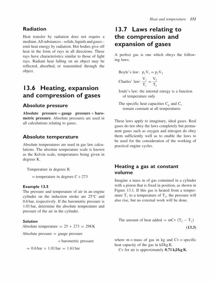
Heat and temperature 151
RadiationHeat transfer by radiation does not require amedium. All substances – solids, liquids and gases –emit heat energy by radiation. Hot bodies give offheat in the form of rays in all directions. Theserays have characteristics similar to those of lightrays. Radiant heat falling on an object may bereflected, absorbed, or transmitted through theobject.
13.6 Heating, expansionand compression of gases
Absolute pressureAbsolute pressure = gauge pressure + baro-metric pressure. Absolute pressures are used inall calculations relating to gases.
Absolute temperatureAbsolute temperatures are used in gas law calcu-lations. The absolute temperature scale is knownas the Kelvin scale, temperatures being given indegrees K.
Temperature in degrees K
= temperature in degrees C+273
Example 13.5The pressure and temperature of air in an enginecylinder on the induction stroke are 25�C and0.6 bar, respectively. If the barometric pressure is1.01 bar, determine the absolute temperature andpressure of the air in the cylinder.
SolutionAbsolute temperature = 25 + 273 = 298 K
Absolute pressure = gauge pressure
+barometric pressure
= 0�6 bar + 1�01 bar = 1�61 bar
13.7 Laws relating tothe compression andexpansion of gases
A perfect gas is one which obeys the follow-ing laws:
Boyle’s law � p1V1 = p2V2
Charles’ law:V1
T1
= V2
T2
Joule’s law: the internal energy is a functionof temperature only
The specific heat capacities Cp and Cv
remain constant at all temperatures
These laws apply to imaginary, ideal gases. Realgases do not obey the laws completely but perma-nent gases such as oxygen and nitrogen do obeythem sufficiently well as to enable the laws tobe used for the consideration of the working ofpractical engine cycles.
Heating a gas at constantvolumeImagine a mass m of gas contained in a cylinderwith a piston that is fixed in position, as shown inFigure 13.1. If this gas is heated from a temper-ature T1 to a temperature of T2, the pressure willalso rise, but no external work will be done.
The amount of heat added = mCv �T2 − T1�
(13.3)
where m = mass of gas in kg and Cv = specificheat capacity of the gas in kJ/kg K.
Cv for air is approximately 0.71 kJ/kg K.

152 Automotive science and mathematics
m
Piston Fixed
Heating atConstant Volume
Heat Added = mCv(T2 – T1) m = Mass of Gas
(a) (b)
Piston MovesExternal Work = p(V2 – V1)
Heating atConstant Pressure
Heat Added = mCv(T2 – T1) + p(V2 – V1) = mCp(T2 – T1)
m
p
p
V2
V1
Fig. 13.1 Heating a gas at constant pressure and constant volume
Heating a gas at constantpressureImagine the same mass, m, of gas in a cylinder fittedwith a movable piston, as shown in Figure 13.1(b)to which heat is applied to raise the temperaturefrom T1 to T2. As the heat is applied the temper-ature of the gas in the cylinder rises but, becausethe piston is able to move, the pressure insidethe cylinder remains constant. In addition to rais-ing the temperature, work is done, by the gas, onthe piston. The amount of heat added in this case is
Q = m Cv �T2 −T1�+work done by the piston
(13.4)
The heat energy required to heat the gas at con-stant pressure is greater than it is when the volumeis constant because of the work done in movingthe piston to maintain the constant pressure. Thisleads to the fact that a greater amount of heat isrequired to raise the temperature of a given massof gas from T1 to T2 at constant pressure thanis required for constant-volume heating becauseof the external work done by the moving piston.The amount of heat required for constant-pressureheating from T1 to T2 is
Q = m Cp �T2 −T1� (13.5)
where Cp = specific heat capacity at constant pres-sure. (Cp for air is approximately 1 kJ/kg K.)
Charles’ lawWhen a gas expands while the temperatureremains constant, the volume divided by the abso-lute temperature is a constant, expressed mathe-matically:
V1
T1
=V2
T2
(13.6)
where the temperatures are absolute K. This rela-tionship is known as Charles’ law, after the sci-entist who first explained it.
Expansion or compressionat constant temperature –isothermalWhen a fixed mass of gas expands or is com-pressed in a cylinder such that the temperatureremains constant, the pressure multiplied by thevolume is a constant. For example:
p1V1= p2V2= C (13.7)

Heat and temperature 153
where the pressures are absolute. This relationshipwas discovered by Robert Boyle in 1661 and it isknown as Boyle’s law (see Figure 13.3).
The graph produced by this type of expansionis a rectangular hyperbola and such expansions ofgases are known as hyperbolic.
General law pVn = C, expansionof gasThis is the type of expansion that occurs in anengine cylinder. During this type of expansionp1V1
n = p2V2n = C, where the pressures are
absolute and the index n lies between 1 and 1.4.
Combined gas lawThis law applies when pressure and temperatureare changing and it is derived from a combinationof Boyle’s and Charles’ laws. The law is
p1V1
T1
= p2V2
T2
where the temperatures and pressures areabsolute. From this equation, it follows thatpV/T = constant. This constant is known as R,the characteristic gas constant, and the equation iswritten as pV = RT. When the mass of gas is m,pV = mRT.
Example 13.6The air in an engine cylinder at the beginning ofthe compression stroke is at atmospheric pressureof 1.02 bar, and a temperature of 23�C. The sweptvolume of the engine cylinder is 450 cm3 and theclearance volume is 50 cm3. If the temperature ofthe air in the cylinder is 80�C at the end of thecompression stroke, calculate the gauge pressureof this air.
SolutionUsing the combined gas law
p1V1
T1
= p2V2
T2
p1 = 1�02 bar� T1 = 273 + 23 = 296 K� T2 =273+80 = 353 K
p2 = p1V1T2
T1V2
V1 = swept volume + clearance volume =450 + 50 = 500 cm3 V2 = clearance volume =50 cm3
∴
V1
V2
= 50050
= 10
p2 = 1�02×10×353296
p2 = 12�16 bar = 12�16−1�02 = 11�14 bar� gauge
Adiabatic expansion pV� = C,expansion of gasWhen a gas expands or is compressed in sucha manner that no heat is added or taken awayfrom the gas the process is said to be adiabatic.In this case the index of expansion is gamma, �,which is the ratio of the specific heats of the gas.Adiabatic processes form the basis for theoreticalengine cycles.
Throttling expansionThis type of expansion occurs when a gasor vapour is forced through a small hole orslightly opened valve. The frictional effect causesthe expanded gas or vapour to become drier, withthe result that the enthalpy (amount of heat) in thesubstance is the same after the throttle as it wasbefore it. This fact is made use of in the expan-sion valve of a vehicle’s air-conditioning system.This valve causes the wet vapour to become dryerbefore entering the evaporator on its way back tothe compressor.
Adiabatic index for airThe adiabatic index for air is the ratio of the spe-cific heat capacities. It is used in connection withthe study of ideal air cycles such as, Otto, Diesel,Dual combustion, and others. The adiabatic indexis denoted by the symbol gamma (�). Taking the
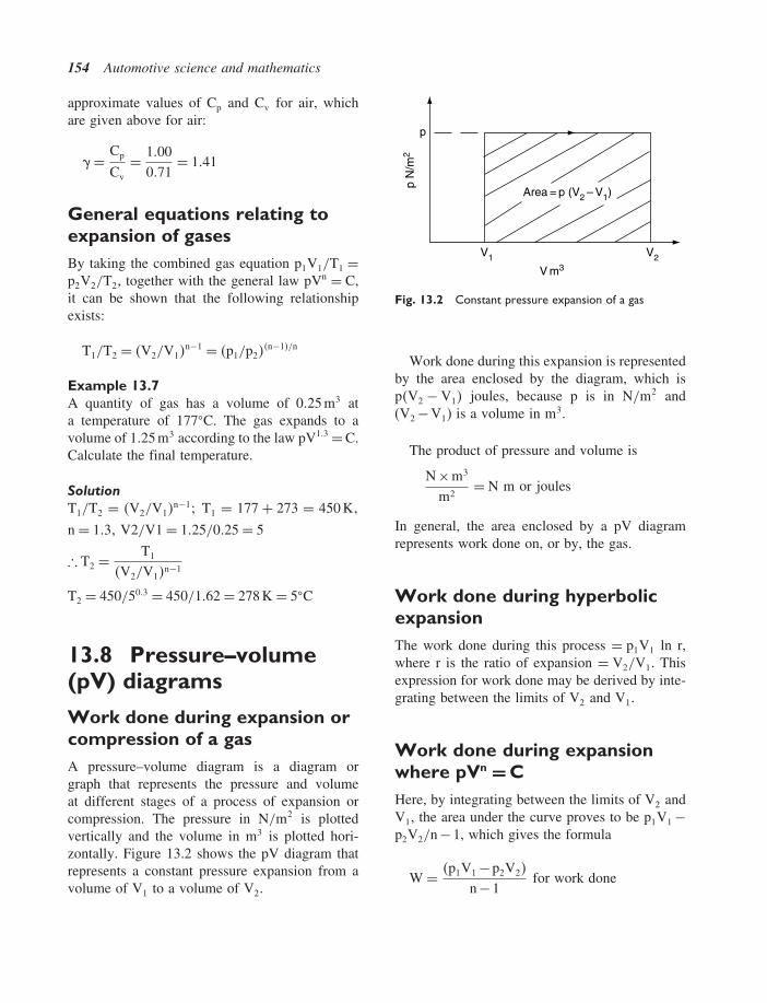
154 Automotive science and mathematics
approximate values of Cp and Cv for air, whichare given above for air:
� = Cp
Cv
= 1�000�71
= 1�41
General equations relating toexpansion of gasesBy taking the combined gas equation p1V1/T1 =p2V2/T2, together with the general law pVn = C,it can be shown that the following relationshipexists:
T1/T2 = �V2/V1�n−1 = �p1/p2�
�n−1�/n
Example 13.7A quantity of gas has a volume of 0�25 m3 ata temperature of 177�C. The gas expands to avolume of 1�25 m3 according to the law pV1�3 = C.Calculate the final temperature.
SolutionT1/T2 = �V2/V1�
n−1 T1 = 177 + 273 = 450 K�
n = 1�3� V2/V1 = 1�25/0�25 = 5
∴ T2 = T1
�V2/V1�n−1
T2 = 450/50�3 = 450/1�62 = 278 K = 5�C
13.8 Pressure–volume(pV) diagrams
Work done during expansion orcompression of a gasA pressure–volume diagram is a diagram orgraph that represents the pressure and volumeat different stages of a process of expansion orcompression. The pressure in N/m2 is plottedvertically and the volume in m3 is plotted hori-zontally. Figure 13.2 shows the pV diagram thatrepresents a constant pressure expansion from avolume of V1 to a volume of V2.
p
Area = p (V2 – V1)
V1 V2
V m3
p N
/m2
Fig. 13.2 Constant pressure expansion of a gas
Work done during this expansion is representedby the area enclosed by the diagram, which isp�V2 − V1� joules, because p is in N/m2 and(V2 −V1) is a volume in m3.
The product of pressure and volume is
N ×m3
m2= N m or joules
In general, the area enclosed by a pV diagramrepresents work done on, or by, the gas.
Work done during hyperbolicexpansionThe work done during this process = p1V1 ln r,where r is the ratio of expansion = V2/V1. Thisexpression for work done may be derived by inte-grating between the limits of V2 and V1.
Work done during expansionwhere pVn = CHere, by integrating between the limits of V2 andV1, the area under the curve proves to be p1V1 −p2V2/n −1, which gives the formula
W = �p1V1 −p2V2�
n −1for work done

Heat and temperature 155
p1
V1 V2
p N
/m2
pV = C
Hyperbolic Expansion
Fig. 13.3 Hyperbolic expansion
Work done during adiabaticexpansion where pV� = CThis is a special case where n = �.
The formula for work done is, thus �
W = �p1V1 −p2V2�
� −1
Example 13.8A quantity of gas has a volume of 2 m3 and apressure of 7 bar. It is expanded in a cylinder untilthe pressure is 0.5 bar. If the barometric pressure is1 bar, calculate the work done if the expansion is:
(a) adiabatic; � = 1�4(b) hyperbolic.
Solution(a) W = �p1V1 −p2V2�/� −1
p1 = 7+1 = 8 barp2 = 0�5+1 = 1�5 bar.V2 is required and is calculated from p2V2
� =p1V1
�V2 = �p1/p2�
1/�
V2 = �8/1�5�1/1�4 ×2= 5�330�714 ×2
V2 = 3�8×2 = 7�6 m3.W = �8×105 ×2−1�5×105 ×7�6�/1�4−1W = �11�4×10⁵�/0�4 = 28�5×105 = 2�85 MJ
(b) W = p1V1 ln r, where r = V2/V1.To obtain V2, use Boyle’s law, p1V1 = p2V2,which gives V2 = p1/p2V1
= �8/1�5�×2 = 10�67 m3.W = 8×10⁵ × ln �10�67/2�
= 8×10⁵ × ln 5�33= 8×105 ×1�67= 13�39×105
= 1�339 MJ
13.9 Summary offormulae
Linear expansion = l �t2 − t1�
Charles’ law – constant pressure:V1
T1
= V2
T2Boyle’s law – constant temperature: p1V1 = p2V2
Combined gas law:p1V1
T1
= p2V2
T2p1V1
n = p2V2n
PV = mRT etc.
W = �p1V1 − p2V2�
�n −1�
� = Cp/Cv
T1/T2= �V2/V1�n−1= �p1/p2�
n−1/n
Degrees K = Celsius temperature + 273
13.10 Exercises
13.1 A certain petrol engine has a compressionratio of 8.5:1. During a compression test,a gauge pressure of 12 bar was recorded.At the start of compression the pressure wasatmospheric at 1 bar and the temperatureof the air in the cylinder was 30�C. Calcu-late the temperature of the air in the cylinderat the end of the compression stroke.
13.2 At the end of the compression stroke, theair in the combustion space of a certainspark ignition engine occupies a space of50 cm3. The pressure in the combustionchamber is 13 bar and the temperature is

156 Automotive science and mathematics
170�C. If the air–fuel ratio is 14.7:1 calcu-late the mass of fuel to be injected. TakeR for air = 0.287 kJ/kg K and assume thebarometric pressure to be 1 bar.
13.3 A certain diesel engine has a compres-sion ratio of 20:1. At top dead centreon the power stroke the gauge pressurein the cylinder is 150 bar. If expansion onthe power stroke takes place according tothe law pV1�3 determine the gauge pressureat the end of this stroke. Atmospheric pres-sure = 1.014 bar.
13.4 A certain diesel engine has a compres-sion ratio of 18:1. In its naturally aspiratedform the air pressure in the cylinder at thecommencement of compression is 1.01 barABS. The engine is adapted to take a turbo-charger and this increases the air pres-sure in the cylinder to 1.7 bar ABS, at thestart of the compression stroke. In bothcases the index of the compression is 1.3.Determine the percentage increase in the airpressure at the end of compression. Takeatmospheric pressure = 1 bar.
13.5 A single-cylinder petrol engine with aswept volume of 500 cm3 has a compres-sion ratio of 9.5:1. As part of an engine con-version, the clearance volume is decreasedto 50 cm3. Calculate:(a) the new compression ratio.(b) in both cases, the gauge pressure of the
air in the cylinder at the end of thecompression stroke if the initial pres-sure is 1.016 bar ABS and the index ofcompression is 1.35.
13.6 A certain turbocharged diesel engine has acompression ratio of 20:1. The air temper-ature in the cylinder at the commencementof the compression stroke is 110�C. If thecompression follows the law pV1�3 = C,calculate the temperature at the end of thecompression stroke. A later version of thisengine has an intercooler that reduces thetemperature of the air in the cylinder, at thecommencement of compression, to 70�C.Calculate the air temperature in the cylinder
at the end of compression in this case andcomment on the effect that this reductionin temperature may have on engine power.
13.7 An engine has a swept volume of 750 cm3
and a compression ratio of 10:1.Calculate:(a) the clearance volume;(b) the work done on a single power stroke
if the pressures are 180 bar at the com-mencement of the power stroke and0.5 bar at the end of the stroke. Takethe barometric pressure = 1 bar and thelaw of expansion as pV1�25 = C.
13.8 When fitting a new ring gear to a flywheel,the ring gear is heated so that the expan-sion produced is sufficient to allow the ringgear to slide on to the periphery of the fly-wheel, and, when the temperature drops,the ring gear will contract and fit tightlyon the flywheel. In order to ensure thatthe hardness of the gear is not impaired, athermo-chromatic coloured pencil is usedto ensure that the ring gear is heated to270�C. If the coefficient of linear expan-sion of the ring gear is 0�000011/�C andthe inner diameter is 300 mm, calculate theincrease in diameter when the ring gear isheated to 270�C from an original tempera-ture of 25�C.
13.9 A certain gudgeon pin has a diameter of20.622 mm at 21�C. It is to be fitted into thesmall end-eye of a connecting rod that hasa diameter of 20.59 mm at 21�C. The rec-ommended procedure for performing thisfitting operation is to heat the connectingrod. If the coefficient of linear expansion ofthe connecting rod is 0�000011/�C, calcu-late the temperature to which the rod mustbe heated in order to achieve the expan-sion of 0.05 mm of the gudgeon-pin eyethat is required for completion of the fittingprocess.
13.10 The cooling system of a certain engine con-tains 6 kg of water. Calculate the quan-tity of heat absorbed by this water whenthe temperature increases from 5�C to

Heat and temperature 157
80�C. Specific heat capacity of water= 4.2 kJ/kg C.
13.11 During a braking operation, the four brakediscs of a motor car absorb 800 kJ ofenergy. If the original operating tempera-ture of the brake discs was 40�C, calculatethe brake discs’ temperature at the end ofthe braking operation. The mass of eachbrake disc is 2.5 kg and the specific heatcapacity of the disc material is 0.5 kJ/kg C.Assume no heat is transferred away fromthe brake discs.
13.12 A certain small petrol engine has a com-pression ratio of 9:1. At the start ofthe compression stroke, the air in thecylinder is at atmospheric pressure andits temperature is 20�C. If the pressurein the cylinder at the end of compressionis 12 bar (gauge), determine the tempera-ture of the compressed air in the cylinder.Atmospheric pressure = 1.016 bar.
13.13 2 m3 of gas at 50�C are heated at constantpressure until the volume is doubled. Deter-mine the final temperature of the gas.

14Internal combustion engines
14.1 Engine power
Brake powerThe engine power that actually reaches the out-put shaft or flywheel of an engine is known asthe brake power. It is the power that is measuredby a dynamometer and a dynamometer is alsoknown as a brake, hence the term, brake power.The simplest form of dynamometer is shown inFigure 14.1. Here a rope is wound around the cir-cumference of the engine flywheel; one end of therope is supported by a spring balance and the otherend has weights attached to it. The load that the
R
W
S
FlywheelCylinder
Fig. 14.1 Simple dynamometer for low-speed engines
engine is working against is varied by increasing,or decreasing, the amount of weight. The effec-tive load (force) that the engine is working againstis = W −S.
Rotating the flywheel inside the rope, againstthe force �W −S� newtons, is equivalent to mov-ing the force �W − S� around the circumferenceof the flywheel. The distance travelled by theforce during one revolution of the flywheel isequal to the circumference of the flywheel. Ifthe radius of the flywheel is R metres, the cir-cumference = 2�R metres. From this, it may beseen that:
Work done per revolution of the flywheel= force ×distance= �W −S�×2�R joules
�W −S�×R also = T� the torque that theengine is exerting. By substituting T for�W −S�×Rthe work done per revolutionbecomes = T ×2� joules
Brake power = work done per second= �T ×2��×number of revolutionsper second
This is normally written as brake powerbp = 2� TN� where N = number ofrevolutions per second�
When the torque is in newton metres (N m), theformula bp = 2� TN gives the power in watts. As

Internal combustion engines 159
engine power is given in thousands of watts, i.e.kilowatts, the formula for brake power normallyappears as:
bp= 2� TN/1000 kW (14.1)
14.2 Dynamometers forhigh-speed engines
Hydraulic dynamometers of the type manufac-tured by the Heenan Froude company are com-monly used for engine testing purposes. Theenergy from the engine is converted into heatby the action of the dynamometer rotors and theaction is somewhat similar to the action of a torque
convertor. Figure 14.2 shows a cross-section of thedynamometer; the engine under test is connectedto the shaft that drives rotor A. Rotor A acts as apump that directs pressurised water into the statorF. The stator is connected to a torque arm that reg-isters the torque acting on it by means of weightsand a spring balance. The power absorption capac-ity of the dynamometer is controlled by means ofa form of sluice gate E that is interposed betweenthe stator F and rotor A. These sluice gates arecontrolled manually. The energy absorbed by thedynamometer is converted into heat in the water,which is supplied under pressure through the inletpipe D.
Electrical dynamometers are also used for high-speed engine testing; these convert the enginepower into electricity which is then dissipatedthrough heat or electro-chemical action.
A
D
E
F
Heenan – Froude Dynamometer
C
B
Fig. 14.2 Hydraulic dynamometer

160 Automotive science and mathematics
Example 14.1A certain engine develops a torque of 120 Nmwhile running at a speed of 3000 rev/min. Calcu-late the brake power. Take � = 3�142.
Solutionbp = 2� TN/1000.
From the question, T = 120 Nm; N = 3000/60= 50 rev/s
Substituting these values in the formula givesbp = 2×3�142×120×50/1000 = 37�7 kW.
14.3 Horsepower
One horsepower = 746 watts. The conversionfrom kilowatts to horsepower is:
Power in kilowatts ÷ 0�746. Taking the aboveexample of 37.7 kW, the horsepower equivalent is37�7 kW ÷0�746 = 50�5 bhp.
14.4 PS – the DIN
The abbreviation PS derives from pferdestrake,which is German for the pulling power of ahorse. 1 PS is slightly less than 1 imperialhorsepower.
14.5 Indicated power
Indicated power (ip) is the power that is devel-oped inside the engine cylinders. It is determinedby measuring the pressures inside the cylinderswhile the engine is on test, on a dynamometer.The device that is used to measure the pressure iscalled an indicator, from which the term indicatedpower is derived. The indicator diagram for a 4-stroke engine is shown in Figure 14.3.
Because the pressure varies greatly throughoutone cycle of operation of the engine, the pressurethat is used to calculate indicated power is themean effective pressure.
Power
Pressure
Exhaust
InductionAtmospherePressure
VolumeBDCTDC
Compression
Fig. 14.3 Indicator diagram for a 4-stroke engine
14.6 Mean effectivepressure
The mean effective pressure is that pressurewhich, if acting on its own throughout one com-plete power stroke, would produce the same poweras is produced by the various pressures that occurduring one operating cycle of the engine.
In Figur 14.4(a), the loop formed by the pres-sure trace for the exhaust and induction strokesis known as the pumping loop. This representspower taken away and the effective area is deter-mined by subtracting A2 from A1. This calculationthen gives the indicated mean effective pressure.The resulting area �A1 −A2� is then divided by thebase length of the diagram. The resulting meanheight is then multiplied by a constant that givesthe indicated mean effective pressure (imep).
Example 14.2An indicator diagram taken from a single-cylinder4-stroke engine has an effective area of 600 mm2.If the base length of the indicator diagram is60 mm and the constant is 80 kPa/mm calculatethe indicated mean effective pressure.
SolutionIndicated mean effective pressure (imep)
= effective area of indicator diagrambase length of the diagram
× constant

Internal combustion engines 161
Power
Comp
Ex
INDBase Length
p barA1
A2
Atmosphere Pressure
Indicator Diagram
(a)
BDCTDC
(b)
�
p Piston Dia A = Area of Piston = πd2
4
� = Length of Stroke in mA = Area of Piston Crown m2
p = Indicated Mean Effective Pressure N/m2
Work Done per Stroke = p × A × � J,if Ns = Number of Working Strokes/s.Power = p × A × � × Ns Watt
Fig. 14.4 Indicated power calculation
imep = 60060
×80 kPa/mm
imep = 800 kPa = 8 bar
14.7 Calculation ofindicated power
Indicated power is calculated from the formula
Indicated power (ip) = PlaN1000
kW
where P = mean effective pressure in N/m2,l = length of engine stroke in m, a = cross-sectional area of cylinder bore in m2, N = numberof working strokes per second.
Example 14.3In a test, a certain single-cylinder 4-stroke enginedevelops a mean effective pressure of 5 bar at aspeed of 3000 rev/min. The length of the enginestroke is 0.12 m and the cross-sectional area of thecylinder bore is 0�008 m2. Calculate the indicatedpower of the engine in kW.
SolutionThe engine is single-cylinder 4-stroke, so thereis one working stroke for every two revolutions.N, the number of working strokes per second= 3000 ÷ 60/2 = 25; P = 5 bar = 500 000 N/m2,l = 0�12 m; a = 0�008 m2.
Substituting these values in the formula gives
ip = 500 000×0�12×0�008×25/1000 kW
= 12 kW

162 Automotive science and mathematics
Number of working (power) strokesAs mentioned, each cylinder of a 4-stroke engineproduces one power stroke for every two rev-olutions of the crankshaft. In a multi-cylinderengine, each cylinder will produce one powerstroke in every two revolutions of the crankshaft.A formula to determine the number of powerstrokes per minute for a multi-cylinder, 4-strokeengine is:
number of power strokes per minute
= number of cylinders2
× rev/min
Example 14.4A 4-cylinder, 4-stroke engine develops an indi-cated mean effective pressure of 8 bar at2800 rev/min. The cross-sectional area of thecylinder bore is 0�01 m2 and the length of thestroke is 150 mm. Calculate the indicated powerof the engine in kW.
SolutionThe required formula is:
ip = PlaN1000
kW
From the question, N, which is the number ofpower strokes per second is
number of cylinders2
× rev/min60
which gives N = 4/2 × 2800/60 = 93�3 persecond.
Length of stroke in metres = 120/1000 =0�12 m
P = 8 bar = 800 000 N/m2
And the area of the piston a = 0�01 m2
Substituting these values in the formula gives:
ip = 800 000×0�12×0�01×93�3÷1000 kW
= 89�6 kW
Because engine power is still frequently quotedin horsepower, it is useful to know that 1 horse-power = 746 watts = 0�746 kW.
This engine’s indicated power is therefore =89�6/0�746 = 120�1 hp.
14.8 Cylinder pressurevs. crank angle
The behaviour of the gas in an engine cylin-der is an area of study that enables engineersto make detailed assessments of the effects ofchanges in engine-design and types of fuel, etc.Devices such as pressure transducers and oscillo-scopes permit cylinder gas behaviour to be exam-ined under a range of engine operating conditions.The basic elements of an indicator that permitthis type of study are shown in Figure 14.5(a).The sparking plug is drilled as shown, and thehole thus made is connected to a small cylin-drical container in which is housed a piezoelec-tric transducer. Gas pressure in the cylinder isbrought to bear on this piezo transducer throughthe drilling in the sparking plug and the smallpipe. Gas pressure on the transducer produces asmall electrical charge that is conducted to anamplifier, which is calibrated to convert an elec-trical reading into an input to the oscilloscope thatrepresents gas pressure. An additional transduceris attached to the engine crankshaft. The elec-trical output from the crank transducer is ampli-fied as necessary and fed to the X input of theoscilloscope.
Figure 14.5(b) shows the type of oscilloscopedisplay that is produced by a high-speed indicator.The display shows part of the compression andpower strokes of a diesel engine. Injection com-mences at point A and combustion starts at pointB; point C represents the end of effective com-bustion. The periods between each of these pointsare the three phases of combustion.

Internal combustion engines 163
(a)
Modified Sparking Plug
Piezo Transducer
Amplifier
YX
Oscilloscope
Crank Angle Sensor
60
50
40
30
20
10
80 70 60 50 40 30 20 10 10 20 30 40 50 60 70 80
Pre
ssur
e B
ar
Compression
B
A
TDCC
Power
Crank Angle Degrees
(b)
Fig. 14.5 (a) A high-speed engine indicator; (b) cylinder pressure vs. crank angle
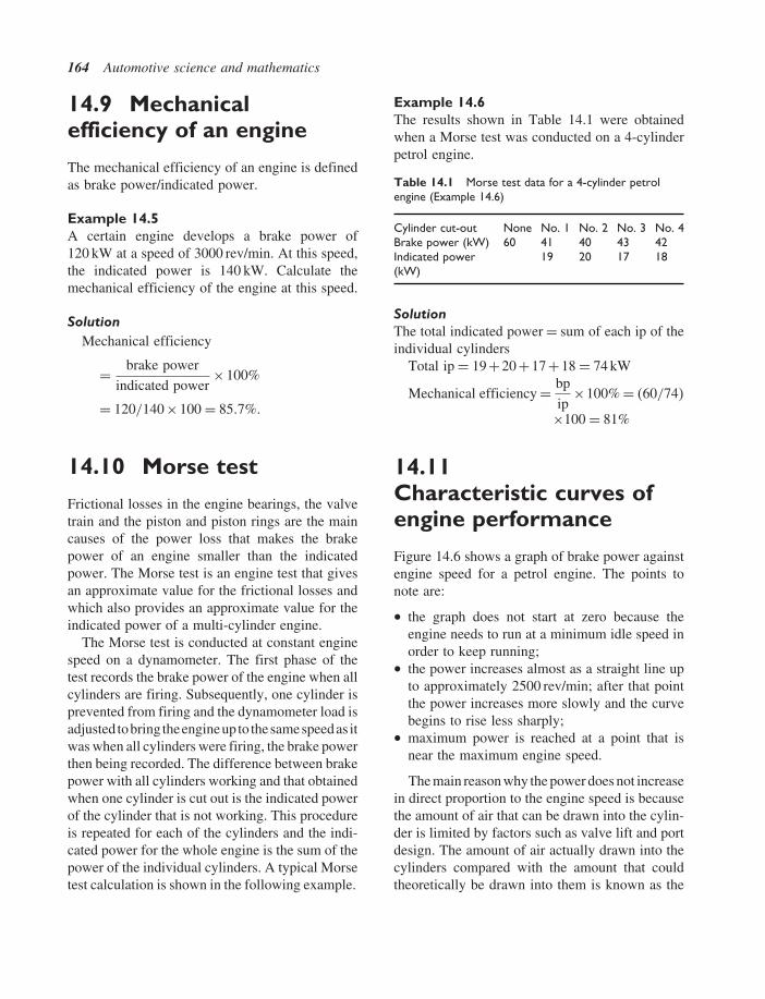
164 Automotive science and mathematics
14.9 Mechanicalefficiency of an engine
The mechanical efficiency of an engine is definedas brake power/indicated power.
Example 14.5A certain engine develops a brake power of120 kW at a speed of 3000 rev/min. At this speed,the indicated power is 140 kW. Calculate themechanical efficiency of the engine at this speed.
SolutionMechanical efficiency
= brake powerindicated power
×100%
= 120/140×100 = 85�7%�
14.10 Morse test
Frictional losses in the engine bearings, the valvetrain and the piston and piston rings are the maincauses of the power loss that makes the brakepower of an engine smaller than the indicatedpower. The Morse test is an engine test that givesan approximate value for the frictional losses andwhich also provides an approximate value for theindicated power of a multi-cylinder engine.
The Morse test is conducted at constant enginespeed on a dynamometer. The first phase of thetest records the brake power of the engine when allcylinders are firing. Subsequently, one cylinder isprevented from firing and the dynamometer load isadjusted tobring theengineup to thesamespeedas itwas when all cylinders were firing, the brake powerthen being recorded. The difference between brakepower with all cylinders working and that obtainedwhen one cylinder is cut out is the indicated powerof the cylinder that is not working. This procedureis repeated for each of the cylinders and the indi-cated power for the whole engine is the sum of thepower of the individual cylinders. A typical Morsetest calculation is shown in the following example.
Example 14.6The results shown in Table 14.1 were obtainedwhen a Morse test was conducted on a 4-cylinderpetrol engine.
Table 14.1 Morse test data for a 4-cylinder petrolengine (Example 14.6)
Cylinder cut-out None No. 1 No. 2 No. 3 No. 4Brake power (kW) 60 41 40 43 42Indicated power(kW)
19 20 17 18
SolutionThe total indicated power = sum of each ip of theindividual cylinders
Total ip = 19+20+17+18 = 74 kW
Mechanical efficiency = bpip
×100% = �60/74�
×100 = 81%
14.11Characteristic curves ofengine performance
Figure 14.6 shows a graph of brake power againstengine speed for a petrol engine. The points tonote are:
• the graph does not start at zero because theengine needs to run at a minimum idle speed inorder to keep running;
• the power increases almost as a straight line upto approximately 2500 rev/min; after that pointthe power increases more slowly and the curvebegins to rise less sharply;
• maximum power is reached at a point that isnear the maximum engine speed.
The main reason why the power does not increasein direct proportion to the engine speed is becausethe amount of air that can be drawn into the cylin-der is limited by factors such as valve lift and portdesign. The amount of air actually drawn into thecylinders compared with the amount that couldtheoretically be drawn into them is known as the

Internal combustion engines 165
1000
20
40
2000 3000
Petrol Engine
Bra
ke P
ower
kW
4000 5000 6000
60
80
100
120
140
160
Fig. 14.6 Brake power vs. engine speed
8001
1200 1600 2000
Engine Speed rev/min
Vol. effy
Vol
umet
ric E
ffici
ency
%
2400 2800 3200 3600 4000
75
80
85
90
Fig. 14.7 Volumetric efficiency – diesel engine
volumetric efficiency. Above a certain speed, vol-umetric efficiency drops and this, coupled withfrictional and pumping losses, affects the amountof power produced. Figure 14.7 shows a graph ofvolumetric efficiency plotted against engine speed.
14.12 Volumetricefficiency
Volumetric efficiency
= volume of charge admitted at STPswept volume
= actual air flowtheoretical air flow
Example 14.7A 4-cylinder 4-stroke petrol engine with a borediameter of 100 mm and a stroke of 110 mm has avolumetric efficiency of 74% at an engine speedof 4000 rev/min. Determine the actual volume ofair at STP that flows into the engine in 1 minute.
SolutionVolumetric efficiency = actual air flow
theoretical air flowTheoretical air flow = swept volume of one
cylinder×number of cylinders× rev/min2
Swept vol. of one cylinder = �d214= 0�7854×0�1×0�1×0�11 m3
= 8�64×10−4 m3
∴ Theoretical volume of air= 8�64×10−4 m3 ×4×4000/2= 6�91 m3/min
Actual air flow= theoretical air flow×volumetric
efficiencyActual air flow = 0�74×6�91 = 5�11 m3/min
14.13 Torque vs. enginespeed
Torque is directly related to brake mean effectivepressure (bmep). The graph in Figure 14.8 shows
1000
50
100
150
200
Engine Speed rev/min
Tor
que
Nm
2000 3000 4000
Fig. 14.8 Torque vs. engine speed

166 Automotive science and mathematics
that torque varies across the speed range of anengine. Torque may be determined by direct mea-surement at a dynamometer, or by calculation;for example
T = brake power2�n
where the brake power is determined by dynamo-meter tests.
14.14 Specific fuelconsumption vs. enginespeed
Brake specific fuel consumption (bsfc) is a mea-sure of the effectiveness of an engine’s ability toconvert the chemical energy in the fuel into usefulwork. Brake specific fuel consumption is calcu-lated as shown, for example
bsfc = mass of fuel consumed per hourbrake power
Figure 14.9 shows how bsfc varies with enginespeed.
1000
100
200
300
400
Engine Speed rev/min2000 3000 4000
Spe
cific
Fue
l Con
sum
ptio
n g/
kwh
Fig. 14.9 Specific fuel consumption vs. engine speed
Example 14.8The results shown in Table 14.2 were obtainedduring a fuel consumption test on an engine.
Table 14.2 Results of fuel consumption test on anengine (Example 14.8)
Brake power(kW)
10 15 20 25 30 35
Total fuelconsumedper hour (kg)
4 5�21 6�74 8�4 10�59 12�6
Determine the specific fuel consumption (sfc)in kg/kWh in each case and plot a graph of specificfuel consumption on a base of brake power.
Brake Power kw0 5 10 15 20 25 30 35
Spe
cific
Fue
l Con
sum
ptio
n kg
/kw
h
0.6
0.5
0.4
0.3
0.2
0.1
0
Fig. 14.10
Solution
Specific fuel consumption
= mass of fuel used per hourbrake power
Table 14.3 Specific fuel consumption calculationsbased on Table 14.2 (Example 14.8)
Brake power(kW)
10 15 20 25 30 35
Specific fuelconsumption(kg/kWh)
0�4 0�347 0�337 0�336 0�353 0�36

Internal combustion engines 167
14.15 Brake power,torque and sfc compared
Inorder toassess the importanceof thesecurves, it isnormal practice to plot brake power, torque and spe-cific fuel consumption on a common base of enginespeed. The vertical scales are made appropriate toeach variable. Figure 14.11 shows such a graph.
The points to note are:
• the maximum power of 52 kW occurs at4000 rev/min;
• the minimum specific fuel consumption of237 g/kWh occurs at 2000 rev/min;
• the maximum torque of 147 N m occurs at2100 rev/min.
This data highlights details that affect vehiclebehaviour; e.g., when the specific fuel consump-tion is at its lowest value the engine is con-suming the least possible amount of fuel for thegiven conditions – this is considered to be themost economical operating speed of the engine.The maximum torque also occurs at approximately
160150
140
130
120
110
100
310
290
270
250
230
1000
10
20
30
40
50
2000
r/min3000 4000
210
Tor
que
Nm
s.f.c
g/kw
h
Pow
erkW
Fig. 14.11 Characteristic curves of diesel enginevariables
the same speed, because torque converts to trac-tive effort; the maximum tractive effort is obtainedat the same engine speed as is found for the max-imum torque speed.
The maximum power is reached at a high enginespeed.
The ratio of maximum power speed to maxi-mum torque speed is known as the engine speedratio.
The most useful part of the power curve of theengine lies between the maximum torque speedand the maximum torque speed. The differencebetween maximum power speed and maximumtorque speed is known as the engine operatingrange.
In this case the engine operating speed range =4000 rev/min −2100 rev/min = 1900 rev/min.
The actual shapes of the graphs of these enginecharacteristics are determined by engine design.The graphs for a heavy transport vehicle enginemay be expected to be quite different from thosefor a saloon car.
14.16 Brake meaneffective pressure
The brake mean effective pressure (bmep) maybe obtained from the brake power curve of theengine as follows: bmep = brake power in kW ×1000 ÷ lan Nm. In this equation, l = length ofengine stroke in metres, a = cross-sectional areaof the cylinder bore in square metres, and n = thenumber of working strokes per second.
When bmep is plotted against engine speed, thecurveproduced is the sameshapeas the torquecurvebecause torque is related to bmep. Engine perfor-mance data such as specific fuel consumption, andits relationship to bmep, at a given engine speed,may be shown in graphical form as in Figure 14.12.Here the engine is run at constant speed, on adynamometer, and the air–fuel ratio is varied.
The main point to note here is that maximumbmep is developed when the mixture is rich.The minimum fuel consumption occurs when the

168 Automotive science and mathematics
500
SFCSFC.
Air-Fuel Ratio (Petrol)10 11 12 13 14 15 16 17 18
bmep.
bmep
. bar
.
10
8
6
4
2
Max power Min SFC
gm/kwh400
300200
Fig. 14.12 Brake mean effective pressure vs. sfc atconstant engine speed
air–fuel ratio is slightly weaker than the chemi-cally correct air–fuel ratio of 14.7:1 for petrol.
14.17 Thermal efficiency
The thermal efficiency of an engine is a term thatis used to express the effectiveness of an engine’sability to convert heat energy into useful work.Thermal efficiency is the ratio of energy outputof the engine to energy supplied to the engine inthe fuel.
Brake thermal efficiency
= brake energy/smass of fuel/s× calorific value of the fuel
Example 14.9During a 10-minute dynamometer test on a petrolengine, the engine develops a brake power of45 kW and uses 3 kg of petrol. The petrol has acalorific value of 43 MJ/kg. Calculate the brakethermal efficiency.
SolutionFuel used per second 3/600 = 0�005 kg/s
1 kW = 1 kJ/s. Brake energy per second =45 kJ/s
Brake thermal efficiency = 45×103 ÷0�005×43×106 = 45 000÷215 000 = 0�209 or 20�9%.
14.18 Indicated thermalefficiency
Indicated thermal efficiency
= indicated energy/smass of fuel/s× calorific value
Example 14.10During a dynamometer test, a certain 4-cylinder,4-stroke diesel engine develops an indicatedmean effective pressure of 8.5 bar at a speed2000 rev/min. The engine has a bore of 93 mmand a stroke of 91 mm. The test runs for 5 minutesduring which time 0.8 kg of fuel are used. Thecalorific value of the fuel is 43 MJ/kg. Calculatethe indicated thermal efficiency.
SolutionIndicated power = P l a NN = number of working strokes/second
= number of cylinders/2× revs/s
= 4/2×2000/60 = 66�7
Length of stroke (l) = 0.091 m
Area of bore (a) = �/4 × 0�093 × 0�093= 0�0068 m2
imep� p = 8�5×10⁵ N/m2
Indicated power
= 8�5×105 ×0�091×0�0068×66�71000 kW= 35�1 kW
Mass of fuel/s = 0�8/300 = 0�0027 kgIndicated thermal efficiency
= 35�1 × 1000 J/s0�0027 × 43 × 106
= 0�302 or 30.2%.
14.19 Brake thermalefficiency petrol vs. diesel
For reasons that are explained in Chapter 15,which deals with engine cycles, the brake ther-mal efficiency of a diesel engine is normally

Internal combustion engines 169
higher than it is for a comparably sized petrolengine. The higher thermal efficiency of thediesel engine results in good fuel economy. Thefigures shown in Table 14.4 refer to two vehi-cles of the same model, one fitted with a dieselengine and the other with a petrol engine of thesame size.
Table 14.4 Fuel economy in petrol and dieselengines
Fuel economy Petrol engine Diesel engine
Urban cyclemiles/US gallon
15 25
Highway cycle 21 34Composite 18 29
14.20 Heat energybalance
In Example 14.9 the engine has a brake thermalefficiency of 20.9%. This means that 20.9% of theenergy supplied to the engine in the fuel is con-verted into useful work. In order to determine whathappens to the remainder of the energy supplied inthe fuel, a heat energy balance test is conducted.The energy balance is conducted under controlledconditions in a laboratory. The test apparatus isequipped with a dynamometer and with meters forrecording air and fuel supply, cooling water flowand exhaust gas temperature.
Energy supplied to the engine= mass of fuel used× calorific value
Energy to the cooling water = mass of water× specific heat capacity× temperatureincrease
Energy to useful work= brake power as measured by
dynamometerSpecific heat capacity of water = 4�18 kJ/kg C
Energy to the exhaust = mass of exhaust gas× specific heat capacity× temperature
increaseSpecific heat capacity of the exhaust gas
= 1�012 kJ/kg C approximatelyMass of fuel used as recorded on a fuel flow
meter = mf kgCalorific value is obtained from the fuel
specificationMass of water flowing through the engine
cooling system = mw kgTemperature rise of cooling water
= Twout−Twin�C
Temperature rise of exhaust gas is recorded bya thermocouple sensor that is placed in theexhaust stream, close to the engine = Texout
−Texin�C
Mass of exhaust gas: this isdetermined by adding the mass of airsupplied to the mass of fuel supplied. Themass of air supplied is determined by theairflow meter through which all air forcombustion passes.
Mass of exhaust gas = mass of air+mass of fuel = mex
Example 14.11The data shown in Table 14.5 was obtained duringa 1-hour laboratory test on an engine.
Construct a heat balance for this engine. Takethe specific heat capacity of the exhaust =1�01 kJ/kg C; specific heat capacity of the water= 4�2 kJ/kg C.
Table 14.5 Data from engine test (Example 14.11)
Brake power 60 kWMass of fuel used 18 kg/hAir used (air fuel ratio = 16:1 by mass) 288 kg/hTemperature of air at inlet 20�CTemperature of exhaust gas 820�CMass of water through cooling system 750 kg/hCooling water temp in 15�CCooling water temp out 85�CCalorific value of fuel 43 MJ/kg

170 Automotive science and mathematics
SolutionHeat energy supplied in the fuel = 18 × 43= 774 MJ/h
Heat energy to the exhaust = �18 + 288�×1�01×103 × �820−20� = 247�25 MJ/h
Heat energy to cooling water = 750 × 4�2×10³ × �85−15� = 252 MJ/h
Heat energy equivalent of brake power = 60×1000×3600 = 216 MJ/h.
Table 14.6 Tabulated results of heat balancecalculations (Example 14.11)
Heat supplied in thefuel/h
774 MJ 100%
Heat to brakepower
216 MJ 28%
Heat to exhaust 247.25 MJ 32%Heat to coolingwater
252 MJ 32.6%
Heat to radiationetc. (by difference)
58.75 MJ 7.4%
CommentThis balance sheet provides a clear picture of theway in which the energy supplied to the engine isused. It is clear that approximately two thirds ofthe energy is taken up by the exhaust and cool-ing system. In turbo-charged engines, some of theexhaust energy is used to drive the turbine andcompressor and this permits the brake power out-put of the engine to rise.
14.21 Effect of altitudeon engine performance
The density of air decreases as the air pressuredecreases and this causes a loss of power in natu-rally aspirated engines when they are operating athigh altitude. It is estimated that this power lossis approximately 3% for every 300 m (1000 ft) ofaltitude. Turbocharged engines are affected to alesser extent by this effect.
14.22 Summary of mainformulae
Volumetric efficiency
= volume of charge admitted at STPswept volume
Brake power (bp) = 2�Tn60×1000
where T is torque in Nm, n = rev/min
Indicated power (ip) = P l a n60×1000
where P = imep in N/m2, l= length of strokein m, a = area of bore in m2, n=number ofworking strokes per min; for 4-stroke engine
n = number of cylinders× rev/min2
Mechanical efficiency = bpip
×100
Brake thermal efficiency
= energy to brake powerenergy supplied in the fuel
= bp×1000×3600mass of fuel/h× cal� val
�
Brake specific fuel consumption
= mass of fuel used per hourbp
14.23 Exercises
14.1 A 4-cylinder, 4-stroke engine with a borediameter of 80 mm and a stroke length of75 mm develops an indicated mean effec-tive pressure of 6.9 bar at an engine speedof 3600 rev/min. Calculate the indicatedpower at this engine speed.
14.2 The results shown in Table 14.7 wereobtained when a Morse test was conducted
Internal combustion engines 171
Table 14.7 Results of a Morse test conducted on a6-cylinder engine (Exercise 14.3)
Cylindercut-out
None No. 1 No. 2 No. 3 No. 4
Brake power(kW)
120 85 87 88 86
on a 6-cylinder engine operating at a con-stant speed of 3000 rev/min. Calculate theindicated power of the engine and themechanical efficiency at this speed.
14.3 (a) Calculate the brake power of a6-cylinder engine that produces a bmep of7 bar at a speed of 2000 rev/min. The boreand strokes are equal at 120 mm. (b) If themechanical efficiency at this speed is 80%,calculate the indicated power.
14.4 A diesel engine develops a brake powerof 120 kW at a speed of 3000 rev/min. Atthis speed the specific fuel consumption is0.32 kg/kWh. Calculate the mass of fuelthat the engine will use in 1 hour underthese conditions.
14.5 As a result of a change in design, thebmep of a 4-cylinder, 4-stroke engine risesfrom 7.5 bar to 8 bar at an engine speedof 2800 rev/min. The bore and stroke are100 mm and 120 mm respectively. Cal-culate the percentage increase in brakepower at this speed that arises from thedesign changes.
14.6 A 6-cylinder, 4-stroke petrol engine devel-ops an indicated power of 110 kW at aspeed of 4200 rev/min, the imep at thisspeed being 9 bar. Calculate the bore andstroke given that the engine is ‘square’, i.e.the bore = stroke.
14.7 An engine develops a torque of 220 Nmduring an engine trial at a steady speed of
3600 rev/min. The trial lasts for 20 min-utes during which time 8.3 kg of fuel areconsumed. The calorific value of the fuelis 43 MJ/kg. Calculate the brake thermalefficiency.
14.8 The data in Table 14.8 shows the resultsof a Morse test conducted on a 4-cylinderengine. Calculate the indicated power andthe mechanical efficiency of the engine.
Table 14.8 Results of a Morse test conducted on a4-cylinder engine (Exercise 14.8)
Cylindercut-out
None No. 1 No. 2 No. 3 No. 4
bp (kW) 25 17 16 18 16
14.9 A 4-cylinder, 4-stroke petrol engine witha bore diameter of 100 mm and a strokeof 110 mm has a volumetric efficiency of70% at an engine speed of 4200 rev/min.Determine the actual volume of airat STP that flows into the engine in1 minute.
14.10 The data in Table 14.9 shows the resultsobtained during a dynamometer test ona 4-cylinder diesel engine. Calculate thebrake thermal efficiency for each value ofbrake power and plot a graph of (a) spe-cific fuel consumption on a base of bpand (b) brake thermal efficiency on thesame base. Calorific value of the fuel= 44 MJ/kg.
Table 14.9 Results obtained during a dynamometertest on a 4-cylinder diesel engine (Exercise 14.10)
bp (kW) 10 20 40 60 80Specific fuelcons.(kg/kWh)
0.32 0.29 0.27 0.28 0.30

15Theoretical engine cycles
Ideal engine cycles such as the Otto cycle, thediesel cycle and others are known as air cyclesbecause the working fluid that drives the engine isassumed to be air. In order to study engine theory,the processes that make up the engine operatingcycle are represented on a graph of pressure andvolume. The graph is referred to as a pV diagram.The pV diagram is, in effect, an indicator diagramfor an ideal engine. Throughout the cycle of oper-ation, the working fluid is assumed to be air, andthe air is assumed to be a perfect gas. The heatis assumed to be introduced by means of a heatsource that is applied to the end of the cylinder,and the residual heat is removed by means of acold source applied to the cylinder.
15.1 The constantvolume cycle (Otto cycle)
The theoretical constant volume cycle was firstproposed by Beau de Rochas in 1862. However,the first working engine that used the Beau deRochas principles was designed by Otto and theconstant volume cycle has been known ever sinceas the Otto cycle. Figure 15.1 shows the pressurevolume indicator diagram for the Otto cycle.
The cylinder is filled with air and the pistonis used to compress this air and to transmit the
3
2
1
4
Adiabatic Compression and Expansion
Constant Volume
Constant Volume
p
V
Piston Moves Along Cylinder
Fig. 15.1 The Otto (constant volume) cycle
work that arises from expansion. Heat is added tothe air by means of a hot source that is attachedto the cylinder; at the low-pressure end of thecycle the remaining heat in the air is removed byattaching a cold source to the cylinder.
Working round the diagram we start at point 1,which corresponds to bottom dead centre in apetrol engine. As the piston is pushed along thecylinder the volume decreases from V1 to V2.The air in the cylinder is compressed adiabaticallyup to point 2, which is top dead centre. Duringthis adiabatic compression no heat is added to theair in the cylinder and none is lost through thecylinder wall – in effect there is no heat energy

Theoretical engine cycles 173
transfer between the air in the cylinder and the sur-roundings. This compression corresponds to thecompression stroke in a petrol engine.
At point 2, the piston has reached the end of itsstroke and heat energy is added to the air in thecylinder. This causes the temperature and pressureof the air in the cylinder to rise to the level rep-resented by point 3. The volume of the air in thecylinder remains constant during this heating ofthe air from T2 to T3. The heat energy is addedby attaching a hot body to the cylinder. The pro-cess corresponds to the combustion phase in apetrol engine.
At point 3, the heat source is removed andthe gas expands adiabatically to point 4, doingwork on the piston in the process. During adia-batic expansion there is no heat transfer betweenthe air in the cylinder and its surroundings. Thisexpansion corresponds to the power stroke in apetrol engine.
At point 4, the remaining energy in the air inthe cylinder is removed, at constant volume, untilthe pressure returns to point 1. This process is per-formed by attaching a cold body to the cylinder.This part of the cycle corresponds to the exhaustphase in a petrol engine.
The useful work done during one cycle is rep-resented by the area enclosed by the pV dia-gram. It can be shown that this useful work isequal to the heat energy supplied to the air in thecylinder between points 2 and 3 minus the heatrejected from this air between points 4 and 1 onthe diagram.
Useful work = mCv�T3 −T2�−mCv�T4 −T1�
where m = mass of air in the cylinder and Cv =specific heat capacity of air at constant volume.
Thermal efficiency of thetheoretical Otto cycle
Thermal efficiency = useful work doneheat energy supplied
Thermal efficiency
� = mCv�T3 −T2�−mCv�T4 −T1�
m Cv�T3 −T2�
� = �T3 −T2�− �T4 −T1�
�T3 −T2�(15.1)
This can be further simplified to give
� = 1− �T4 −T1�
�T3 −T2�
Thermal efficiency in termsof compression ratio rBy using the relationship T1/T2 = �V2/V1�
n−1
= �p1/p2��n−1�/n, and the fact that the compres-
sion ratio r = V1/V2, the temperatures T1, T2, T3
and T4 can be expressed in terms of r. For exam-ple T1 = T2�1/r��−1. When these substitutions aremade, the equation
thermal efficiency
= 1− �T4 −T1�
�T3 −T2�can be expressed as
thermal efficiency = 1− 1r�−1
The thermal efficiency that is calculated from thisformula is known as the air standard efficiency ofan engine operating on the Otto cycle.
Air standard efficiency = 1− 1r�−1
(15.2)
where � = adiabatic index for air, r = compressionratio.
Example 15.1A petrol engine operating on the Otto cycle hasa compression ratio of 8:1. Given the adiabaticindex for air � = 1�41, calculate the air standardthermal efficiency.

174 Automotive science and mathematics
SolutionAir standard thermal efficiency
� = 1− 1r�−1
r = 8� � = 1�41
� = 1− 180�41
= 1−0�43
ASE � = 0�57 = 57%
The ideal, or air standard, efficiency is 57%.This result shows that the larger r becomes, thesmaller the fractional part of the thermal efficiencyequation becomes and this results in higher ther-mal efficiency.
Effect of compression ratioon thermal efficiencyA graph of thermal efficiency plotted against com-pression ratio for an Otto cycle engine shows howthe effect of increased compression ratio affectsthermal efficiency (Figure 15.2). For the lowercompression ratios in the range 5:1 to 10:1, a small
2 4 6 8 10 12 14 16
10
20
30
40
50
60
70
Compression Ratio
Idea
l Effi
cien
cy %
Fig. 15.2 Relationship between ideal thermal efficiencyand compression ratio
increase in compression ratio leads to a markedincrease in ideal efficiency.
The air standard efficiency is the efficiency thatan Otto cycle engine could achieve should theideal conditions be achieved, and it thus serves asa benchmark against which practical engines canbe compared.
15.2 Relative efficiency
Relative efficiency = actual thermal efficiencyair standard efficiency
(15.3)
Example 15.2The following results were obtained during atest to determine the indicated thermal efficiencyof an engine: indicated power 50 kW, fuel usedper hour = 15 kg. Calorific value of the fuel =43 MJ/kg. Engine compression ratio = 8:1; � =1�41. Calculate:
(a) the indicated thermal efficiency;(b) the air standard efficiency;(c) the relative efficiency.
Solution(a) Indicated thermal efficiency
= energy of indicated powerenergy supplied in fuel
Energy of indicated power = 50 kJ/s
Energy supplied in fuel
= mass of fuel/second
× calorific value
= �15/3600�×43 MJ/s
= 179�17 kJ/s
∴ Indicated thermal efficiency
= 50 kJ/s179�17 kJ/s
= 0�28 = 28%

Theoretical engine cycles 175
(b) Air standard efficiency (ASE)
= 1− 1r�−1
= 1− 180�41
= 1−0�43
= 0�57 = 57%
(c) Relative efficiency
= actual thermal efficiencyair standard efficiency
= 0�280�57
= 0�49 = 49%
15.3 Diesel or constantpressure cycle
In the theoretical diesel cycle the pressure–volumediagram is of the form shown in Figure 15.3.
Heat Added at Constant Pressure = mCp(T3 – T2)
Theoretical Diesel Cycle
3
4
1
2
v
p
Fig. 15.3 pV diagram for the diesel cycle
Working round the diagram, starting at point 1: airis compressed adiabatically – no heat is added tothe air in the cylinder and none is rejected, up topoint 2. At point 2, heat energy is added and the airin the cylinder expands, doing work on the piston;the volume increases to point 3 while the pres-sure remains constant. Work is done on the pistonduring this phase. No further heat is added afterpoint 3 and the air in the cylinder expands adia-batically doing work on the piston up to point 4.At point 4 the remaining heat energy in the air inthe cylinder is removed while the volume remainsconstant and the air in the cylinder is restored toits original state at point 1.
Because the compression and expansion pro-cesses are adiabatic, during which no heat is addedor rejected, the work done during the cycle = heatadded – heat rejected.
The air standard thermal efficiency of the diesel
cycle = heat added – heat rejected
heat added
= mCp�T3 −T2�−mCv�T4 −T1�
mCp�T3 −T2�
= 1− 1�T4 −T1�
��T3 −T2�
By using the relationship T1/T2 = �V2/V1�n−1 =
�p1/p2��n−1�/n, and the fact that the compression
ratio r = V2/V1, the thermal efficiency of thiscycle, which is also known as the air standardefficiency, can be shown to be:
ASE = 1− ��� −1�
���−1�· 1
r�−1(15.4)
where r is the compression ratio, � is a factorderived from the fuelling design of the engine,and � = adiabatic index for air.
Example 15.3A certain diesel engine has a compression ratio of14:1. The fuelling factor � = 1�78. Calculate theair standard efficiency; take � = 1�4.

176 Automotive science and mathematics
SolutionASE = 1− ���−1�
���−1�· 1
r�−1
Taking r = 14, � = 1�78, � = 1�4
ASE = 1− �1�781�4 −1�
1�4�1�78−1�· 1
140�4
= 1−0�396
= 0�604 = 60�4%
15.4 The dualcombustion cycle
Large, low-speed (100 rpm) diesel engines suchas those used for marine propulsion or stationarypower generation operate reasonably closely tothe ideal diesel cycle. However, smaller, lighter-weight engines that are necessary for road vehiclesare required to operate at higher speeds and it isconsidered that the modified diesel cycle knownas the dual combustion cycle more accurately rep-resents the thermodynamic processes that occur inhigh-speed compression ignition engines.
Operation of dual combustioncycleIn this cycle, the pV diagram of which is shownin Figure 15.4, the combustion takes place in twostages, one at constant pressure and one at con-stant volume. Working round the diagram frompoint 1, which corresponds to bottom dead centreon the compression stroke, the air in the cylinderis compressed adiabatically up to point 2. At point2 heat is added, increasing the pressure while thevolume remains constant until point 3 is reached.At point 3 further heat is added at constant pres-sure, expansion taking place up to point 4. Frompoint 4 to point 5, the air in the cylinder expandsadiabatically. At point 5 the remaining heat isremoved at constant volume to restore the air toits original condition ready to repeat the cycle.
Heat Added at Constant Volume = mCv(T3 – T2)Heat Added at Constant Pressure = mCp(T4 – T3)
4
5
1
3
2
p
v
Fig. 15.4 pV diagram for the dual combustion cycle
During the adiabatic compression and expansionprocesses no heat is added or rejected, and thework done during the cycle = heat added – heatrejected.
The air standard efficiency of the engine oper-ating on this cycle = work done ÷ heat supplied.
Air standard efficiency
= heat added−heat rejectedheat added
= mCv�T3 −T2�+mCp�T4 −T3�−mCv�T5 −T1�
mCv�T3 −T2�+mCp�T4 −T3�
This expression can, by substitution, be shownto be
ASE = 1−1×Fr�−1
(15.5)
where r is the compression ratio and F is a factorderived from the fuelling arrangements for theengine.
Example 15.4A compression ignition engine operating on thedual combustion cycle has a compression ratio of16:1. The fuelling factor F for this engine is 1.2.Use Equation (15.5) to calculate the ideal thermalefficiency of this engine and take � = 1�4.

Theoretical engine cycles 177
SolutionFrom Eqn (15.5), ideal thermal efficiency (ASE)
= 1− 1×Fr�−1
= 1− 1×1�2150�4
= 1− �0�338×1�2�
= 1−0�41
= 0�59 = 59%
15.5 Comparisonbetween theoretical andpractical engine cycles
Some of the factors that are taken into accountwhen comparing practical engine cycles with the-oretical ones are as follows.
• The air and combustion gases in the cylinderare not perfect gases.
• Adiabatic processes are not realised in practice.• Instantaneous application and removal of heat
energy are practically impossible.
The diagrams in Figure 15.5(a–c) are reasonablerepresentations of actual engine cycles. In both theOtto cycle diagram and the diesel and dual com-bustion cycle diagrams the principal differencebetween the theoretical and the actual is the loopat the bottom of the diagram. This loop arises fromthe exhaust and induction strokes. The exhauststroke expels heat from the cylinder and it replacesthe constant volume heat rejection of the theo-retical cycle. The other part of this loop arisesfrom the induction stroke. This loop formed bythe exhaust and induction strokes is known as thepumping loop. The area of this loop representswork done by the air in the cylinder and when sub-tracted from the loop formed by the compression,power and heat addition parts of the diagram, theeffective area of the diagram is reduced. This leads
p
EX
Induction
Power
Com
pressionV
4 Stroke Otto Cycle (Actual)(a)
(b)
(c)
AtmosphericPressure
EX
IND
PowerComp
p
p
V4 Stroke Diesel (Actual)
PowerComp
EX
INDV
4 Stroke Dual Combustion (Actual)
Fig. 15.5 Indicator diagram for (a) petrol engine; (b) low-speed diesel engine; (c) high-speed diesel engine – dualcombustion.
to a considerable difference in power producedper stroke of the actual cycle compared with thetheoretical one. These, and similar considerations,lead to the main differences between the efficien-cies of practical engines and those produced bycalculations based on ideal cycles.

178 Automotive science and mathematics
15.6 The Stirling engine
The Stirling engine operates by external combus-tion. The air in the hermetically sealed enginecylinder is heated by means of a heat exchangerknown as a regenerator, as opposed to fuel beingburned in the cylinder. The original Stirling enginewas designed by the Revd Stirling in 1845. Stirlinghot-air engines were used in some industrial appli-cations and domestic appliances, but have droppedout of use because steam engines have proven tobe more effective. In the twentieth century, severalmanufacturers worked on the development of Stir-ling engines for use in motor vehicles because theyshould ideally produce fewer harmful emissions
and have a higher thermal efficiency comparedwith conventional engines.
The Stirling engine regeneratorThe air, or gas, that drives the engine is enclosed ina casing that includes the regenerator. Figure 15.6shows a simplified form of regenerator that con-sists of a heater, a cooler, and a wire gauze heatsink. The closed-cycle working air is pumped fromend to end of the regenerator by means of thecompressor section of the engine. Heat is appliedexternally from the heater section, this causing thetemperature of the engine air to rise to T1; the air inthe engine expansion cylinder is thus heated, caus-ing it to expand and provide engine power. Heat
Coldwater
WireGauze
Cooler
T2 (Low)
T1 (High)
Fuel
Heater
Air to and from Engine
Air to and from Engine
Fig. 15.6 A simplified Stirling engine regenerator

Theoretical engine cycles 179
passes through the wire gauze to the cooler end ofthe regenerator and heat is stored in the wire gauzeduring the process; the working air at the coolend of the regenerator has a lower temperature ofT2. During another part of the engine operatingcycle, the working air is pumped back throughthe regenerator, from the cool end to the hot end.During this process the working air regains heatfrom the gauze.
A double-acting Stirling engineThe engine shown in Figure 15.7 has two double-acting cylinders that are interconnected via theregenerators at the ends of each cylinder. Theworking gas that is sealed inside the engine systemmay be air, or some other gas such as nitrogen;it is constantly heated and expanded and cooledand compressed as the pistons reciprocate in the
Hot
Cool
Cool
Heater
Heater
Cooler
Gauze
Hot
Piston Rod
B
A
Working Gas Sealedwithin the System
Regenerator
Regenerator
Swash PlateMechanism
Cooler
Fig. 15.7 Double-acting Stirling engine

180 Automotive science and mathematics
cylinders. The reciprocating linear motion of thepiston rods is converted to rotary motion by meansof the swash plate. As shown in Figure 15.7, theheated gas is forcing piston A down the cylinder.At the same time the cooler, lower-pressure gasbelow piston A is being forced through the regen-erator where it is reheated as it enters the othercylinder below piston B. At the same time, thecooler gas above piston B is being forced throughthe top regenerator into the cylinder above pistonA. The power output of the engine is determinedby the amount of heat energy that is applied atthe heater part of the regenerator. The pressure–volume diagram for an engine working on thisideal cycle is shown in Figure 15.8. The heatingand cooling of the working gas takes place at con-stant volume, and the expansion and compressionprocesses are isothermal. The thermal efficiencyof this ideal engine is given by the expression
� = T1 −T2
T1
(15.6)
This is the same as the Carnot efficiency whichis, in theory, the highest efficiency that can beachieved by any heat engine. One attraction of theStirling engine is the prospect of achieving a very
p
V
T2
T1
Isothermal
Isothermal Comp
ConstantVolume
ConstVol
Exp
Fig. 15.8 Ideal Stirling cycle
high thermal efficiency; another is the fact thatexternal combustion permits a wide range of fuelsto be used.
Example 15.5A test on Stirling engine produced the followingresults: air at 1 bar pressure and temperature of25�C is compressed isothermally and then heatedat constant volume until the pressure is 9 bar andthe temperature is 300�C. Calculate the thermalefficiency.
SolutionThe highest temperature T1 = 300+273 = 573 K
The lowest temperature T2 = 25+273 = 298 K
Thermal efficiency � = T1 −T2
T1
= 573−298573
= 0�48 = 48%
15.7 The gas turbine
While several designs of heavy vehicle have usedgas turbine engines of the type used in aircraft,the early promise of these engines has not mate-rialised and the principal use of gas turbinesin road transport is in the turbocharger, whichhas found widespread application. The constant-pressure type of gas turbine engine utilises acompressor to compresses air prior to fuel beinginjected to increase its temperature. The heated airthen passes into the turbine where the energy ofthe stream of gas is converted to rotational energythat drives the power shaft.
The theoretical cycle for the constant-pressuregas turbine cycle is shown in Figure 15.9b.

Theoretical engine cycles 181
Heat In
Comp Exp
Adiabatic
(a)
(b)
Exhaust
V
p
c
ad
b
Turbine
Exhaust
Combustion Chamber
PowerShaft
Compressor
Air In
Compr
esse
d Air
Fig. 15.9 (a) The gas turbine; (b) constant pressure gas turbine cycle
Working round this diagram from point a, airis drawn into the compressor where it is com-pressed adiabatically up to point b. At point b thecompressed air is heated by fuel being burned inthe combustion chamber; this heating continues topoint c. From point c the hot gas expands adia-batically through the turbine where it is convertedinto rotational energy at the power shaft. At theend of expansion the remaining heat is removedat constant pressure in the exhaust, shown as d toa on the pV diagram.
The thermal efficiency of this ideal cycle
= heat added−heat rejected
heat added
= mCp�Tc−Tb�−mCp�Td −Ta�
mCp�Tc−Tb�
= 1− �Td −Ta�
�Tc−Tb�
By using the relationship between the pressure,volume and temperature of a gas this equation for

182 Automotive science and mathematics
thermal efficiency can be expressed in terms ofcompression ratio and the adiabatic index for air.
Thermal efficiency of constant pressure
gas turbine = 1− 1r�−1
(15.7)
where r = compression ratio of the compressorand � = adiabatic index for air.
The compressor is attached to the same shaftas the turbine and a considerable amount of tur-bine power is used in driving the compressor. Thepower available to drive machinery or to propela vehicle = turbine power – compressor power.Example 15.6 gives an indication of the perfor-mance of gas turbine plant.
Example 15.6A test on a gas turbine power plant produced thefollowing results:
Work done by turbine = 248�24 kJ/kg of fuelWork done by compressor = 192�56 kJ/kg of fuelEnergy supplied in fuel = 334 kJ/kg of fuel.
Calculate the thermal efficiency of the plant.
SolutionThermal efficiency = useful energy output
energy input
The useful energy output
= turbine energy− compressor energy
= �248�24−192�56� kJ/kg
= 55�68 kJ/kg
Energy input = energy supplied in fuel= 334 kJ/kg
Thermal efficiency = 55�68334
= 16�7%
15.8 Summary offormulae
Thermal efficiency Otto (constant volume) cycle
� = 1− �T4 −T1�
�T3 −T2�
Air standard efficiency Otto cycle = 1− 1r�−1
Relative efficiency = actual thermal efficiencyair standard efficiency
Diesel cycle air standard efficiency ASE
= 1− �� −1�
��−1�· 1
r�−1
Compression ignition engine – dual combustion
cycle efficiency ASE = 1− 1×Fr�−1
Carnot and Stirling engine theoretical cycle
efficiency � =T1 −T2
T1
Thermal efficiency of constant-pressure gas
turbine = 1− 1r�−1
15.9 Exercises
15.1 A single-cylinder 4-stroke petrol enginehas a bore of 79 mm and a stroke of100 mm; the clearance volume is 60 cm3.Calculate:(a) the compression ratio;(b) the air standard thermal efficiency; take
� for air = 1.41.15.2 A heavy-duty oil-engine operating on the
constant-pressure diesel cycle has a com-pression ratio of 15:1. Given � = 1�2 and� = 1�4, calculate the ideal air standard effi-ciency of the engine.
15.3 An indirect-injection diesel engine witha compression ratio of 22:1 operates onthe dual combustion cycle. Given that thefuelling factor F = 1.2 and � = 1�4, cal-culate the ideal air standard efficiency ofthe engine.
15.4 The gas turbine engine of a certain motorvehicle has an actual thermal efficiency of18%. The fuel consumption of the turbine is0.013 kg/s. If the calorific value of the fuelis 43 MJ/kg, calculate the power available topropel the vehicle.

Theoretical engine cycles 183
15.5 Go to the turbokart.com website and studythe description that is given for the AGT1500 gas turbine, which is a power unit forthe M1 American battle tank. Also, use yoursearch engine to look at Rover Gas Turbineat allpart.com, which gives a clear descrip-tion of a Chrysler gas turbine engine.
15.6 The following results were obtained duringa test to determine the indicated thermal effi-ciency of an engine: indicated power 110 kW,fuel used per hour = 30 kg. Calorific valueof the fuel = 43 MJ/kg. The engine compres-sion ratio = 8:1; � = 1�41. Calculate:(a) the indicated thermal efficiency;(b) the air standard efficiency;(c) the relative efficiency.
15.7 A certain 4-stroke petrol engine has a com-pression ratio of 9:1. During a test on adynamometer the engine returns an indicatedthermal efficiency of 28%. Calculate:(a) the air standard efficiency of the engine;(b) the relative efficiency.Take � = 1�41.
15.8 A 4-cylinder 4-stroke petrol engine has abore of 120 mm and a stroke of 110 mm. Ifthe compression ratio is 8:1 determine:(a) the clearance volume;(b) the air standard efficiency.
15.9 Sketch the indicator diagrams for the idealOtto cycle and the ideal diesel cycle.Describe the main differences between thetwo cycles.

16Fuels and combustion & emissions
16.1 Calorific value
The calorific value of a fuel is the amount ofenergy that is released by the combustion of1 kg of the fuel. Two figures for calorific valueof hydrocarbon fuels are normally quoted, thesebeing the higher or gross calorific value, and thelower calorific value. These two values derivefrom the steam that arises from the combustionof hydrogen. The higher calorific value includesthe heat of the steam whereas the lower calorificvalue assumes that the heat of the steam is notavailable to do useful work. The calorific valuethat is quoted for motor fuels is that which is usedin calculations associated with engine and vehi-cle performance. For example, the calorific valueof petrol is approximately 44 MJ/kg. The approx-imate values of the properties of other fuels areshown in Table 16.1.
Table 16.1 Approximate values of fuel properties
Property LPG Petrol Diesel oil Methanol
Relative density 0.55 0.74 0.84 0.8Usable calorific value 48 MJ/kg 44 MJ/kg 42.5 MJ/kg 20 MJ/kgOctane rating 100 90 – 105Chemical composition 82% C; 18% H2 85% C ; 15% H2 87% C; 12.5% H2; 0. 5% S 38% C;12% H2 ; 50% O2
Air–fuel ratio 15.5 14.7 14.9 6.5Mass of CO2 per kg offuel used (kg/kg)
3.04 3.2 3.2 1.4
16.2 Combustion
Modern fuels for motor vehicles, such as petroland diesel fuel, are principally hydrocarbons. Thatis to say that they consist largely of the two ele-ments, hydrogen and carbon. The proportions ofthese elements in the fuel vary, but a reasonablyaccurate average figure is that motor fuels suchas petrol and diesel fuel are approximately 85%carbon and 15% hydrogen.
Products of combustionWhen considering products of combustion it isuseful to take account of some simple chemistryrelating to the combustion equations for carbonand hydrogen.
An adequate supply of oxygen is required toensure complete combustion and this is obtainedfrom atmospheric air.

Fuels and combustion & emissions 185
Relevant combustion equationsFor carbon, C+O2 = CO2. Because of the relativemolecular masses of oxygen and carbon this maybe interpreted as: 1 kg of carbon requires 2.67 kgof oxygen and produces 3.67 kg of carbon dioxidewhen combustion is complete.
For hydrogen, 2H2 + O2 = 2H2O. Again,because of the relative molecular masses of H andO2 this may be interpreted as: 1 kg of hydrogenrequires 8 kg of oxygen and produces 9 kg of H2Owhen combustion is complete.
16.3 Air–fuel ratio
Petrol has an approximate composition of 15%hydrogen and 85% carbon. The oxygen for com-bustion is contained in the air supply and approxi-mately 15 kg of air contains the amount of oxygenthat will ensure complete combustion of 1 kg ofpetrol. This means that the air-to-fuel ratio forcomplete combustion of petrol is approximately15:1; a more precise figure is 14.7:1.
Petrol engine combustionCombustion in spark ignition engines such asthe petrol engine is initiated by the spark at thesparking plug and the burning process is aidedby factors such as combustion chamber design,temperature in the cylinder, and mixture strength.
Because petrol is volatile each element of thefuel is readily supplied with sufficient oxygenfrom the induced air to ensure complete com-bustion when the spark occurs. Petrol enginecombustion chambers are designed so that thecombustion that is initiated by the spark at thesparking plug is able to spread uniformly through-out the combustion chamber.
For normal operation of a petrol engine, a rangeof mixture strengths (air/fuel ratios) are requiredfrom slightly weak mixtures – say 20 parts air toone part of petrol for economy cruising, to 10 parts
of air to one part of petrol for cold starting. Duringnormal motoring, a variety of mixture strengthswithin this range will occur; for example, accel-eration requires approximately 12 parts of air to 1part of petrol. These varied conditions plus otherfactors such as atmospheric conditions that affectengine performance lead to variations in combus-tion efficiency, and undesirable combustion prod-ucts known as exhaust emissions are produced.Exhaust emissions and engine performance areaffected by conditions in the combustion cham-ber; two effects that are associated with combus-tion in petrol engines are (1) detonation and (2)pre-ignition.
DetonationDetonation is characterised by knocking and lossof engine performance. The knocking arises afterthe spark has occurred and it is caused by regionsof high pressure that arise when the flame-spreadthroughout the charge in the cylinder is uneven.Uneven flame-spread leads to pockets of highpressure and temperature that cause elements ofthe charge to burn more rapidly than the mainbody of the charge. Detonation is influenced byengine design factors such as turbulence, heatflow, and combustion chamber shape. The qualityof the fuel, including octane rating, also has aneffect. Detonation may lead to increased emissionsof CO and NOx and HC. result.
Pre-ignitionPre-ignition is characterised by a high-pitched‘pinking’ sound, which is emitted when com-bustion occurs prior to the spark, this beingcaused by regions of high temperature. Thesehigh-temperature zones may be the result of spark-ing plug electrodes overheating, sharp or roughedges in the combustion region, carbon deposits,and other factors. In addition to loss of power andmechanical damage that may be caused by the

186 Automotive science and mathematics
high pressures generated by pre-ignition, combus-tion may be affected and this will cause harmfulexhaust emissions.
16.4 Octane rating
The octane rating of a fuel is a measure of thefuel’s resistance to knock. A high octane numberindicates a high knock resistance. Octane ratingsare determined by standard tests in a single-cylinder, variable compression ratio engine.The research octane number (RON) of a fuel isdetermined by running the test engine at a steady600 rpm while the compression ratio is increaseduntil knock occurs. The motor octane number(MON) is determined by a similar test, but theengine is operated at higher speed. The RON isusually higher than the MON and fuel suppliersoften quote the RON on their fuel pumps. Analternative rating that is sometimes used gives afigure which is the average of RON and MON.
16.5 Compressionignition
In order to produce the high temperature ofapproximately 400�C that is required to ignite thediesel fuel, the air in the cylinder is compressedto a high pressure of approximately 50 bar. Air atthis pressure is dense and the fuel that is injectedinto the cylinder is broken down into minute par-ticles each of which must penetrate the air chargein order to obtain the oxygen for combustion andto provide uniform burning.
Traditionally, compression ignition enginecombustion has been considered to take place inthe three phases identified by Sir Harry Ricardo.These three phases are as follows:
1. The delay period, phase A to B in Figure 16.1.This is the period between the commencementof injection to the beginning of the pressurerise. During this period the fuel droplets are
E
A
B
C D
60
50
40
30
20
10
–60° –40° –20° 20° 40° 60° 80°Crank Angle
TDC
Phases of Combustion
Pre
ssur
e –
Bar
–80°
Fig. 16.1 The three phases of combustion in a CI engine
absorbing the heat from the air in the cylinderthat will lead to combustion.
2. B to C represents the amount of luminouscombustion before TDC; this luminous com-bustion carries on after TDC and is shownin Figure 16.1 as C to D, the flame-spreadperiod. As combustion proceeds and the flamespreads through the charge and more of the fueldroplets are ignited, the pressure rises rapidly.The rate of pressure rise during this phase is amajor cause of the knock that is a characteristicof compression ignition engines.
3. D to E represents the phase where fuel contin-ues to burn.
Compression ignition enginecombustion chambersDiesel (CIE) engines are classified accord-ing to the type of combustion chamber used,namely direct injection and indirect injection(Figure 16.2).
Direct injectionA major part of the combustion space is providedby the specially shaped cavity that is formed in

Fuels and combustion & emissions 187
Cylinder Head Injector
CylinderBlock
Piston CylinderBlock
Piston
Port
Injector
Chamber
(a) (b)
Fig. 16.2 Direct and indirect injection
the piston crown. This cavity is designed to pro-vide swirl, which assists in the combustion. Fuelis sprayed into the combustion space at high pres-sure in excess of 180 bar. Multi-hole injectors arenormally used to ensure maximum spread of thefuel throughout the compressed air.
In the direct injection engine, swirl is normallyproduced in two planes, vertical and horizontal.The piston is very close to the valves and cylinderhead at top dead centre and the small clearancebetween the top of the piston and the lowest partof the cylinder head is known as the ‘bumpingclearance’.
Indirect injectionIndirect injection diesel engines are equipped withan additional small chamber into which the fuel isinjected. This chamber is known as a pre-chamberand is connected to the main combustion chamberof the engine by means of a small-diameter hole.The pre-chamber is designed to produce swirl sothat good combustion is achieved.
16.6 Diesel fuel
Diesel fuel has a calorific value of approximately45 MJ/kg and it has a specific gravity of approxi-mately 0.8 g/cc. The ignition quality of diesel fuelis denoted by the cetane number; a figure of 50indicates good ignition properties. Among other
properties of diesel fuel that affect normal oper-ation are flash point, pour point and cloud point,or cold filter plugging point.
Flash pointThe flash point of a fuel is the lowest temperatureat which sufficient vapour is given off to causetemporary burning when a flame is introducednear the surface. A figure of 125�F (52�C) mini-mum is quoted in some specifications. The flashpoint is determined by means of apparatus suchas the Pensky–Martin flash point apparatus andthe test is performed under controlled laboratoryconditions.
Pour pointThe pour point of a fuel is the temperature atwhich a fuel begins to thicken and congeal andcan no longer be poured. A pour point of 0�For −18�C is suitable for some conditions.
Cloud pointThe cloud point, which is sometimes known asthe cold filter plugging point (CFPP), is the tem-perature at which the fuel begins to have a cloudyappearance and will no longer flow freely througha filtering medium. Cloud point occurs at a tem-perature of approximately 20�F (11�C) above thecloud point temperature.

188 Automotive science and mathematics
Note These figures for diesel fuel are approx-imate and are presented here as a guide only.Readers who require more detailed informationare advised to contact their fuel supplier.
16.7 Exhaust emissions
Exhaust gases are the products of combustion.Under ideal circumstances, the exhaust productswould be carbon dioxide, steam (water) and nitro-gen. However, owing to the large range of oper-ating conditions that engines experience, exhaustgas contains several other gases and materials suchas those given below:
• CO – due to a rich mixture and incompletecombustion;
• NOx – due to very high temperature;• HC – due to poor combustion;• PM – soot and organo-metallic materials;• SO2 – arising from combustion of small amount
of sulphur in diesel fuel.
Factors affecting exhaustemissionsDuring normal operation, the engine of a roadvehicle is required to operate in a number of quitedifferent modes, as follows:
• modes of road vehicle engine operation;• idling – slow running;• coasting;• deceleration – overrun braking;• acceleration;• maximum power.
These various modes of operation give rise tovariations in pressure, temperature and mixturestrength in the engine cylinder with the result thatexhaust pollutants are produced.
HydrocarbonsHydrocarbons (HC) appear in the exhaust as a gasand arise from incomplete combustion due to a
lack of oxygen. The answer to this might seem tobe to increase the amount of oxygen to weaken themixture. However, weakening the mixture givesrise to slow burning, combustion will be incom-plete as the exhaust valve opens and unburnt HCwill appear in the exhaust gases.
IdlingWhen the engine is idling the quantity of fuel issmall. Some dilution of the charge occurs because,owing to valve overlap and low engine speed,scavenging is poor. The temperature in the cylin-ders tends to be lower during idling and thisleads to poor vaporisation of the fuel and HC inthe exhaust.
Coasting, overrun brakingUnder these conditions the throttle valve is nor-mally closed. The result is that no, or very little,air is drawn into the cylinders. Fuel may be drawnin from the idling system. A closed throttle leadsto low compression pressure and very little air;the shortage of oxygen arising from these condi-tions causes incomplete combustion of any fuelthat enters the cylinders and this results in hydro-carbon gas in the exhaust.
AccelerationExamination of torque V specific fuel con-sumption for spark ignition engine reveals thatmaximum torque occurs when the specific fuelconsumption is high. Because the best accelerationis likely to occur at the maximum engine torque, aricher mixture is required in order to produce satis-factory acceleration; fuelling systems provide thistemporary enrichment of appropriate increasesin mixture strength to meet demands placed onthe engine. This leads to a temporary increase inemissions of HC and CO. As the engine speedrises, combustion speed and temperature increaseand this gives rise to increased amounts of NOx.
High-speed, heavy load runningHere the engine will be operating at or near maxi-mum power. Examination of the power V specific

Fuels and combustion & emissions 189
TheoreticalAir-FuelRatio
CO (%) HC(PPM)
HC
CO
NOx
NOx (PPM)
3000
2000
1000
222018161412100
200
400
60012
8
4
0
Richer Air-Fuel Ratio Leaner
Fig. 16.3 Relationship between air–fuel ratio and exhaust emissions
fuel consumption shows that maximum poweris produced at higher specific fuel consumptionfigures and richer mixtures. Increased emissionsof CO and HC are likely to result.
Cruising speed – light engine loadUnder these conditions wherein the engine is prob-ably operating at a low specific fuel consumptionspeed, the mixture strength is likely to be around16:1 or higher to provide good fuel economy.Other emissions are lower under these conditions(Figure 16.3).
16.8 European emissionsstandards
In Table 16.2 are shown the European emissionslimits standards as per EURO 4.
In addition to these standards, modern vehi-cles must be equipped with on-board diagnostics
Table 16.1 EURO 4 emissions limitsstandards (g/km)
CO HC HC + NOx NOx PM
Petrol 1.0 0.10 – 0.08 –Diesel 0.50 – 0.30 0.25 0.025
PM= particulate matter.
(OBD) that notify the driver of the vehicle that asystem malfunction is causing the emissions limitsto be exceeded.
Emissions and their causesOxides of nitrogen (NOx)Oxides of nitrogen are formed when combustiontemperatures rise above 1800 K.

190 Automotive science and mathematics
Hydrocarbons (HC)Unburnt hydrocarbons arise from:
• unburnt fuel remaining near the cylinder wallsafter incomplete combustion being removedduring the exhaust stroke;
• incomplete combustion due to incorrect mixturestrength.
Carbon monoxide (CO)CO emissions are caused by incomplete combus-tion arising from lack of oxygen.
Sulphur dioxide (SO2)Some diesel fuels contain small amounts ofsulphur, which combines with oxygen duringcombustion. This leads to the production of sul-phur dioxide which can, under certain conditions,combine with steam to produce sulphurous acid�H2SO3�, which is a corrosive substance.
Particulate matter (PM)The bulk of particulate matter is soot, which arisesfrom incomplete combustion of carbon. Other par-ticulates arise from lubricating oil on cylinderwalls and metallic substances from engine wear.Figure 16.4 gives an indication of the compositionof particulate matter.
Carbon
Fuel
Lubricant
SO4 + H2O
Fig. 16.4 Approximate composition of particulate matter
Carbon dioxide (CO2)While CO2 is not treated as a harmful emission,it is thought to be a major contributor to thegreenhouse effect and efforts are constantly beingmade to reduce the amount of CO2 that is pro-duced. In the United Kingdom the quantity ofCO2 that a vehicle produces in a standard testappears in the vehicle specification, so it is pos-sible to make comparisons between vehicles onthis score. The figure is presented in grams perkilometre; for example a small economy vehi-cle may have a CO2 figure of 145 g/km anda large saloon car a figure of 240 g/km. Differen-tial car tax rates are applied to provide incentivesto users of vehicles that produce smaller amountsof CO2.
16.9 Methods ofcontrolling exhaustemissions
Two approaches to dealing with exhaust emissionssuggest themselves:
1. Design measures to prevent harmful emis-sions being producedIn diesel engines, such measures includeimproved fuel quality, fuel injection in a num-ber of electronically controlled stages, betteratomisation of fuel such as occurs at higherinjection pressures such as those used in com-mon rail fuel injection systems, and exhaust gasrecirculation.
In petrol engines the approach is some-what similar. Lean-burn engines employingdirect petrol injection is a development that hasbecome reasonably well established. Exhaustgas recirculation is widely used, as is variablevalve timing to overcome the combustion prob-lems caused by valve overlap at idling speed.
2. Post combustion – exhaust emission controlIn diesel engines this consists of catalyticconvertors to oxidise CO and HC, reduction

Fuels and combustion & emissions 191
Electroniccontrol
unit
CONTROL OF EXHAUST-GAS RECIRCULATION
Engine speedTemperature
Air quantityThrottle position sensor
EGR VACUUM VALVE
THE VACUUM OPERATED EGR VALVE
Solenoid
To EGRvalve
Vacuumfrom intakemanifold
Electricalcontrolfrom ECM
Exhaust gas in
Valve raised by vacuum
Vacuum chamber
Diaphragm and EGRvalve return spring
EGR CONTROL VALVETo manifoldvacuum viaEGR solenoidvalve EGR
tointake
SOLENOIDVALVE (EGR)
Exhaust
EGR pipe
EGR pipe
EGR
Air intake
Fig. 16.5 Exhaust gas recirculation system
catalysts to reduce NOx, and particulate filtersto remove particulate matter.
Petrol engines utilise 3-way catalysts andcomputer-controlled fuelling systems. Othertechnologies such as evaporative emissionscontrol, to eliminate HC emission from thefuel system, are also used.
Exhaust gas recirculationThe air that is used to provide the oxygen forcombustion contains approximately 77% nitrogenby mass. When nitrogen is heated above approxi-mately 1800 K (1527�C), in the presence of oxy-gen, oxides of nitrogen �NOx� are formed. Theseconditions occur in the combustion chamber whenexcess oxygen is present as happens at an air–
fuel ratio of approximately 16:1. If the combustionchamber temperature is kept below 1800 K theconditions for the creation of NOx no longer exist.Exhaust gas recirculation is a method that is usedto keep combustion chamber temperatures belowthe critical figure. A proportion of exhaust gas isredirected from the exhaust system to the induc-tion system by means of electronically controlledvalves. Figure 16.5 shows the layout of an enginemanagement system that incorporates exhaust gasrecirculation.
CatalystsCatalysts are materials that assist chemical reac-tions but are not themselves changed in theprocess.

192 Automotive science and mathematics
PlatinumAt the correct temperature, in excess of 300�C,platinum acts as a catalyst that aids the conver-sion of CO to CO2, and HC to H2O and CO2. Inorder for the exhaust system catalytic convertorto function correctly, the air–fuel ratio is main-tained close to that which is chemically correct(stoichiometric) by means of exhaust gas sensorsand electronic control.
RhodiumRhodium is a catalyst that reduces NOx to N2.
These metals are added to a ceramic honey-comb structure that exposes the exhaust gasesto the maximum area of the catalysing material.Figure 16.6 shows the layout of an emission con-trol system for a petrol engine vehicle.
Selective reduction catalystsThe power output of diesel engines is controlledby the quantity of fuel that is injected and theseengines operate with excess air over much of theoperating range. Excess air and high combustiontemperatures give rise to NOx. The selective cata-lyst reduction system (SCR) is a methodology thatis used in heavy vehicles to reduce NOx emissions.
A liquid such as urea is introduced into theexhaust stream where it works in conjunction witha catalytic converter to change NOx into nitrogengas and H2O (water vapour).
Diesel particulate filtersParticulate matter that arises from combustion indiesel engines consists mainly of particles of car-bon with some absorbed hydrocarbons. Filtrationof the exhaust products is a technique that iswidely used for the removal of particulate mat-ter from exhaust gases before they are passedinto the atmosphere. Various forms of filteringmedium are used to trap the PM and, in com-mon with most filtering processes, cleaning of thefilter to avoid blockage is required. The clean-ing process in diesel particulate filters (DPFs),which consists primarily of controlled burning toconvert the carbon (soot) into carbon dioxide, isknown as regeneration. Among the methods ofregeneration are:
Passive systems The heat in the exhaust gas, act-ing with the materials used in the constructionof the particulate filter, produces sufficient tem-perature to remove the filtered deposits. Exter-nal sources of heat are not required.
Active systems Heat is supplied either by inject-ing fuel into the exhaust stream, or by sec-ondary injection of fuel into the engine; this
FuelControl
Electron1 es
NOx
CO HC
O2 SensorO2 Sensor
3 Way Catalyst
CO2 H2O
N2
Petrol Engine Emission Control
Fig. 16.6 A 3-way catalyst emission control system

Fuels and combustion & emissions 193
HCCO
NOxPM
Oxidation Catalyst
Urea InjectionSystem (Reagent)
N2CO2
SCR
Diesel Engine Emission Control
H2O
Fig. 16.7 Selective catalyst reduction (SCR) system
creates the temperature that is required to burnoff the particulate matter that accumulates in thefilter.
16.10 Biofuels
It is currently generally accepted that the world’soil resources are finite and that they are beingdepleted at a rapid rate. Attention is concentratingon alternative fuels and methods of propulsion formotor vehicles. Alcohols such as methyl alcohol,or methanol as it is commonly known, is producedfrom vegetable matter. Biofuels are said to beenvironmentally valuable because their productsof combustion are, very roughly, H2O and CO2.It is argued that the CO2 from the combustion ofthese fuels is consumed by the vegetation that isproducing the crop that, in turn, will make thenext supply of fuel – this process is referred to asa ‘closed carbon cycle’.
Methanol is not strictly a hydrocarbon becauseit contains some oxygen. The calorific value ofmethanol is approximately 26 MJ/kg. It has ahigher latent heat value than that of petrol andhigher resistance to detonation. While the higherlatent heat value and relatively high ignition tem-perature of methanol indicate that higher compres-sion ratios can be used, there is a disadvantage inthat vaporisation at low temperatures is poor andthis can lead to poor cold starting capability.
16.11 Liquefiedpetroleum gas (LPG)
Petroleum gases such as butane and propane areproduced when oil is refined to produce liquidfuels such as diesel (derv) and petrol. Once lique-fied and stored under pressure, LPG will remainliquid until is exposed to atmospheric pressure.The chemical composition of propane is C3H8 andthat of butane, C4H10; the relative densities at 15�Care approximately 0.5 and 0.57 respectively whilethe calorific value is slightly higher than that ofpetrol at approximately 46 MJ/kg. A considerableindustry exists to support the conversion of roadfuelling from petrol and diesel (derv) to LPG. Insome countries, including the UK, favourable taxsystems support the use of LPG.
16.12 Hydrogen
Compressed hydrogen may be stored on a vehicleand used in an internal combustion engine.Among the advantages claimed for it are thatthere are no carbon dioxide emissions and thatthe products of combustion are primarily water.The main future use of hydrogen as a propellantfor vehicles is thought to be as a source of energyin fuel cells. The electricity produced in thesecells is used as a power source for an electricmotor replacing the internal combustion engine

194 Automotive science and mathematics
Electrolyte Membrane
e–e–
e–
e– e–
H+
H+
H+Oxygen O2
Cathode
Water
Anode
HydrogenH2
H2O
Electrical Power
Fig. 16.8 A simple fuel cell
of the vehicle. A simple fuel cell is shown inFigure 16.8. It consists of two electrodes, ananode and a cathode, that are separated by anelectrolyte. Hydrogen acts on the anode andoxygen from the atmosphere acts on the cathode.The catalytic action of the anode causes thehydrogen atom to form a proton and an electron;the proton passes through the polymer electrolyteto the cathode and the electron passes throughan external circuit to the cathode. This actionprovides an electric current in external circuit. Inthe process the hydrogen and oxygen combine toproduce water, which is the principal emission.
16.13 Zero emissionsvehicles (ZEVs)
The operation of fuel cells for vehicle propulsiondoes not involve combustion in an engine and
the normal products of combustion and associatedpollutants are not produced. The main productof the electrochemical processes in the fuel cellis water, and consequently vehicles propelled byfuel cells and electric motors are known as zeroemissions vehicles.
Exercises
16.1 Describe with the aid of sketches the proce-dure and the equipment required to converta fuel injection petrol engine so that it willoperate satisfactorily on LPG.
16.2 Assess the advantages of methanol as amotor fuel and describe the modificationsto a vehicle and its fuel system that maybe required when converting from petrol tomethanol.

Fuels and combustion & emissions 195
16.3 Sketch and describe an exhaust gasrecirculation system.
16.4 Sketch and describe an exhaust gas oxygensensor. Explain how such a sensor is usedto help control exhaust emissions whenused in conjunction with a 3-way catalyst.
16.5 Describe a selective catalyst reduction sys-tem that is used on some diesel vehicles tohelp reduce NOx emissions.
16.6 Enter the Johnson–Matthey website andstudy the various exhaust treatment tech-niques that are described there.
16.7 Compare exhaust gas recirculation andselective catalyst reduction as two alterna-tive methods of reducing NOx emissions.Pay particular attention to initial costs,weight of equipment, maintenance factors,
effect on engine power, and availability ofurea as a reagent, and mention any otherfactors that you think should be considered.
16.8 With the aid of sketches, describe a low-emissions hybrid vehicle that makes use ofa diesel engine and electric motor propul-sion.
16.9 Describe a vehicle that uses hydrogen as agas to provide the fuel to run an adapted4-stroke engine.
16.10 Conduct some research to satisfy yourselfabout the effect on fuelling requirementsthat arise when considering the merits anddemerits of converting a spark ignitionengine to run on alcohol fuel. Pay particularattention to the calorific value and generaleffect on engine performance.

17Electrical principles
17.1 Electric current
An electric current is a flow of electrons througha conductor such as a copper wire.
17.2 Atoms andelectrons
All materials are made up of atoms. An atom has anucleus around which one or more electrons cir-cle in different orbits. An electron has a negativeelectric charge and a nucleus has a positive one.
The electrons orbit around the nucleus inrings that are known as shells, as shown inFigure 17.1(a). The hydrogen atom has a cen-tral nucleus and a single orbiting electron.Figure 17.1(b) shows another type of atom whichhas a nucleus and six electrons. Two of the elec-trons orbit around an inner circle and the otherfour around an outer circle.
The electrons in the outer shells are less stronglyattracted to the nucleus than are those closer toit. These outer electrons are can be moved out oftheir orbit and they are called free electrons.
It is the movement of free electrons thatcauses an electric current. Free electrons occurin most metals.
e–
Orbit
Hydrogen Atom
(a)
+
e–
e–
e
e
e
e
Electrons in Outer Shell
Outer Shell
(b)
+
Fig. 17.1 The atom and electron orbits
17.3 Conductors andinsulators
ConductorsMaterials in which free electrons can be made tomove are known as conductors. Most metals aregood conductors.

Electrical principles 197
1018
1012
10–2
10–8
Insu
lato
rsS
emi-C
ondu
ctor
s
Res
istiv
ity
Con
duct
or
Cer
amic
Sili
caIn
sula
ters
Sili
con
Gal
lium
Ars
enid
eM
etal
sP
ure
and
Allo
yed
Fig. 17.2 Relative conductivity scale for various materials
SemiconductorsSemiconductors are materials whose free elec-trons’ ability to move falls between that of con-ductors and insulators.
InsulatorsMaterials in which free electrons are not readilymoved are known as insulators.
The relative conductivities of various materialsare shown in Figure 17.2.
17.4 Electromotive force
The force that moves free electrons is called anelectromotive force (emf). The symbol E is usedto denote emf and it is measured in volts (V).
Electromotive forces are produced by powersources and there are three principal types ofpower source:
1. chemical – batteries;2. magnetic – generators (alternators and dyna-
mos);3. thermal – thermocouples; used in temperature
measurement.
17.5 Electrical powersources – producingelectricity
Chemical power sourceThe wet cell shown in Figure 17.3(a) consists oftwo plates made of different metals to which areattached the terminals (poles). The liquid whichsurrounds the metal plates is called the electrolyteand it conducts electricity. The electric potential(voltage) at the terminals is caused by a chem-ical reaction between the metal plates and theelectrolyte.
Magnetic power sourceFigure 17.3(b) shows the basic elements ofa dynamo. When the loop of wire is moved ina circular motion between the poles of a magnetthe electric potential difference (volts) exists atthe two ends of the loop.
Thermal power sourceFigure 17.3(c) shows two wires of different met-als, such as copper and iron, that are twistedtogether at one end. When the twisted end isheated, a small emf exists at the opposite ends ofthe wires. This type of device is called a thermo-couple and it is used to measure high temperaturessuch as the temperature of exhaust gas emittedfrom an engine.

198 Automotive science and mathematics
N
S
(a) (c)(b)
Terminals+ –Casing
Electrolyte
Cell
MetalPlates
Thermo-Couple
Bunden
Twisted Meter
Fig. 17.3 Sources of electricity
17.6 Effects of electriccurrent – using electricity
1. Heating effect When electric current flowsthrough a conductor, the conductor heats up.This effect is seen in electric-fire elements,light bulbs (lamps) and similar devices.
2. Chemical effect The main battery on a vehi-cle makes use of the chemical effect of anelectric current to maintain its state of charge,and to provide a source of electric current asrequired.
3. Magnetic effect The magnetic effect of an ele-ctric current is made use of in componentssuch as starter motors, alternators, solenoidsand ignition coils, and in many other devices.
17.7 Electrical circuits
In order to make use of a power source it must beconnected to a circuit.
Circuit principlesThe symbols shown in Figure 17.4 are used torepresent circuit components such as batteries andswitches.
A simple circuitThe electrical pressure at any point in an electricalsystem is called the potential. The potential differ-ence (p.d.) is the difference in electrical pressurebetween two points in an electrical system. Whentwo points of different p.d. are joined togetherby an electrical conductor an electric current willflow between them.
The circuit shown in Figure 17.5 consists of acell (battery) that is connected to a lamp (bulb)and a switch by means of conducting wires. Whenthe switch is closed (on), the emf (voltage) atthe battery will cause an electric current to flowthrough the lamp and the switch, back to the cell,and the lamp will illuminate.
Points to noteA potential difference between two points in acircuit can exist without a current. Current cannotexist in a circuit without a potential difference.
Direction of current flowBy convention, electric current flows fromhigh potential (+, positive) to low potential(−, negative).

Electrical principles 199
Name of Device
Lamp (Bulb)
Diode
Transistor (npn)
Light Emitting Diode(LED)
Switch
Conductors (Wires)Crossing
Conductors (Wires)Joining
Zener Diode
Light DependentResistor (LDR)
Battery
Electric Cell
Resistor
Variable Resistor
Potentiometer
Capacitor
Inductor (Coil)
Transformer
Fuse
(a) A Selection of Circuit Symbols
Symbol Name of Device Symbol
(b) Non-Standard Circuit Symbols
Approved Symbol Symbol Sometimes Used
Fuse
Lamp (Bulb)
Fuse
Lamp (Bulb)
Fig. 17.4 Circuit symbols

200 Automotive science and mathematics
Lamp
Cell
Cable
Switch+–
Fig. 17.5 Simple circuit
17.8 Electrical units
VoltPotential difference and electromotive force ismeasured in volts (V).
AmpereCurrent – Electric current is measured in amperes(A), and it is the number of electrons that passthrough a cross-section of the conductor in 1 sec-ond. The symbol used for electric current is I.
OhmResistance – All materials resist the passage ofelectricity to some degree. The amount of resis-tance that a circuit, or electrical component, offersto the passage of electricity is known as the resis-tance. Electrical resistance is measured in ohmsand it is denoted by the symbol �.
WattPower in a circuit is measured in watts. It is cal-culated by multiplying the current in the circuitby the voltage applied to it.
Power in watts = volts× amperes
W = V× I (17.1)
Example 17.1An electrical component has a current of 5 A flow-ing through it. If the voltage drop across the com-ponent is 10 V, calculate the power used by thecomponent.
W = V× I
= 10×5
Power in watts = 50 W�
17.9 Ohm’s law
Figure 17.6 shows a circuit that can be used toexamine the relation between current, voltage andresistance in a circuit when the voltage is var-ied while the resistance and its temperature areheld constant.
The graph in Figure 17.6(b) shows how the cur-rent increases as the voltage is raised. This graphshows that the current in this circuit is directlyproportional to the voltage producing it, providedthat the temperature of the circuit remains con-stant. This statement is known as Ohm’s law andit is normally written in the form
V = I ×R (17.2)
where V = voltage, I = current in amperes, and Ris the resistance in ohms.
A
VariableVoltageSource D.C
(a) (b)
V R I
V
G
Fig. 17.6 Ohm’s law circuit

Electrical principles 201
17.10 Resistors in series
Example 17.2Figure 17.7(a) shows a circuit that has a 12-voltsupply and two resistors that are connected by aconducting cable. When resistors are connectedas shown, they are in series and the resistance ofthe circuit is found by adding the two resistancevalues together.
In this case R = R1 +R2
R = 4 �+8 �
R = 12 �
Ohm’s law can now be applied to find the currentin the circuit.
Transposing Equation (17.2) gives I = VR
I = 12 V12 �
I = 1 A
In Fig. 17.7(b), the total resistance R
= R1 +R2 +R3
R = 3 �+5 �+10 �
R = 18 �
The current in this case is I = VR
= 1218
I = 0�67 A
8Ω 3Ω 5Ω 10Ω4Ω
R1 R2 R2R1 R3
+ 12V D.C. –(a) (b)
+ 12V D.C. –
Fig. 17.7 Resistors in series
In a series circuit the current is the same inall parts of the circuit.
17.11 Resistors inparallel
Example 17.3Figure 17.8 shows a circuit in which two resistorsare placed in parallel. This ensures that the samep.d. (voltage) is applied to each resistor.
Ohm’s law can be used to find the current ineach resistor as follows:
For resistor R1� I1 = VR1
= 126
I1 = 2 A
For resistor R2� I2 = VR2
= 124
I2 = 3 A
The total current drawn from the supply
I = I1 + I2 = 2+3 = 5 A
R1 = 6Ω
R2 = 4Ω
12V+ –
Fig. 17.8 Resistors in parallel

202 Automotive science and mathematics
17.12 Alternativemethod of finding totalcurrent in a circuitcontaining resistorsin parallel
The equivalent series resistance of the resistors inparallel can be found as follows:
Let R = the equivalent series resistance; then1R
= 1R1
+ 1R2
Using the rules for fractions, the equivalentseries resistance
R = R1 R2
R1 +R2
Example 17.4The circuit in Figure 17.8 has the two resistorsR1 = 6 � and R2 = 4 � in parallel.
Using Equation (17.2), the equivalent series resis-tance R
= 6×46+4
= 2410
R = 2�4 �
To find the current in the circuit, I = VR
= 122�4
I = 5 A
17.13 Measuring currentand voltage
The ammeter measures current and it is connectedin series, so all of the current in the circuit flowsthrough it.
The voltmeter is connected in parallel and itmeasures the potential difference between the two
V
A
CurrentFlow
Fig. 17.9 Ammeter and voltmeter connected to a circuit
points to which it is connected. The p.d. betweentwo points is sometimes referred to as the voltagedrop (Figure 17.9).
17.14 Ohmmeter
An ohmmeter is essentially an ammeter that hasbeen adapted to measure resistance (Figure 17.10).The ohmmeter operates by applying a small volt-age by means of a battery incorporated into themeter. The current flowing is then recorded on ascale that is calibrated in ohms (�).
R
mA9V
TestProbes
Fig. 17.10 Principle of the ohmmeter
17.15 Open circuit
An open circuit occurs when there is a break inthe circuit (Figure 17.11). This may be caused bya broken wire or a connection that has workedloose.

Electrical principles 203
BrokenWire
Switch
Fig. 17.11 Open circuit
17.16 Short circuit
A short circuit occurs when the conducting partof a wire comes into contact with the return sideof the circuit. Because electric current takes thepath of least resistance, the short circuit takes thecurrent back to the battery, and therefore the lampshown in Figure 17.12 will not function.
Short Circuit
Fig. 17.12 Short circuit
17.17 Temperaturecoefficient of resistance
When pure metals such as copper, iron and tung-sten are heated, the resistance increases. Theamount that the resistance rises for each 1�C risein temperature is known as the temperature coef-ficient of resistance.
Res
ista
nce
Ohm
s
Temperature °CVariation of Resistance of Copper with Temperature
–3000
1
2
–200 –100 0 100 200
Fig. 17.13 Temperature coefficient of resistance
Negative temperaturecoefficientWhen some semiconductor ceramic materials areheated, their resistance decreases. For each degreerise in temperature there is a decrease in resis-tance. These materials are said to have a negativetemperature coefficient (Figure 17.14) and theyare used in temperature sensors in various vehi-cle systems.
Res
ista
nce
kΩ
Temperature °C
10
20
020 40 60
Fig. 17.14 Negative temperature coefficient
17.18 Electricity andmagnetism
Permanent magnetsPermanent magnets are found in nature. Mag-netite, which is also known as lodestone, is

204 Automotive science and mathematics
naturally magnetic and ancient mariners used itas an aid to navigation. Modern permanent mag-nets are made from alloys. One particular perma-nent (hard) magnetic material named ‘alnico’ isan alloy of iron, aluminium, nickel, cobalt, anda small amount of copper. The magnetism that itcontains arises from the structure of the atoms ofthe metals that are alloyed together.
Magnetic force is a natural phenomenon. Todeal with magnetism, rules about its behaviourhave been established. Those that are important toour study are related to the behaviour of magnetsand the main rules that concern us are as follows:
• Magnets have north and south poles.• Magnets have magnetic fields.• Magnetic fields are made up from lines of mag-
netic force.• Magnetic fields flow from north to south.
If two bar magnets are placed close to each other sothat the north pole of one is close to the south poleof the other, the magnets will be drawn together. Ifthe north pole of one magnet is placed next to thenorth pole of the other, the magnets will be pushedapart. This tells us that like poles repel each other,and unlike poles attract each other (Figure 17.15).
Attract
S N
S N
S N
SN
Repel
Attraction and Repulsion of Magnets
Fig. 17.15 Effect of magnetic poles
The magnetic effect of anelectric currentFigure 17.16 shows how a circular magnetic fieldis set up around a wire (conductor) which is car-rying electric current.
Lines of Force(Magnetic Flux) Direction of
Current Flow
Fig. 17.16 Magnetic field of straight conductor
Direction of the magnetic fielddue to an electric current in astraight conductorWhen a right-hand-threaded bolt is screwed into anut, or a screw into a piece of wood, the screw isrotated clockwise (this corresponds to the direction,north to south, of the magnetic field); it penetratesthe wood and this corresponds to the direction ofthe electric current in the conductor. The field runsin a clockwise direction and the current flows intowards the wood, as shown in Figure 17.17.
This leads to a convention for representing cur-rent flowing into a conductor and current flowingout (Figure 17.18). At the end of the conductor
F = Field
I = Current
M = Motion
Fig. 17.17 Right-hand-screw rule

Electrical principles 205
+
In Out
Fig. 17.18 Convention for current direction
where current is flowing into the wire, a ‘+’ isplaced, this representing an arrowhead. At the oppo-site end of the wire, where current is flowing out, adot is placed, this representing the tip of the arrow.
Magnetic field caused by a coilof wireWhen a conductor (wire) is made into a coil, themagnetic field created is of the form shown inFigure 17.19(a). A coil such as this is the basis ofa solenoid.
17.19 Solenoid and relay
The solenoid principle is used to operate a relay(Figure 17.19(b)). Relays are used in vehicle sys-tems where a small current is used to control alarger one. When the switch in the solenoid cir-cuit is closed, current flows through the solenoidwinding and this causes the magnetic effect topull the armature towards the soft iron core. Thisaction closes the contacts of the heavy currentswitch to operate a circuit, for example a vehicleheadlamp circuit. When the relay solenoid cur-rent is switched off, the magnetic effect dies awayand the control spring pulls the armature awayfrom the soft iron core to open the heavy currentswitch contacts.
17.20 Electromagneticinduction
Figure 17.20 shows a length of wire that has avoltmeter connected to its ends. The small arrowspointing from the north pole to the south pole
Direction ofCurrent FlowN
S
(a)
(b)
SwitchContacts
Armature Return Spring
Fig. 17.19 (a) Magnetic field of a coil; (b) relay
of the magnet, represent lines of magnetic force(flux) that make up a magnetic field.
The straight arrow on the wire (conductor)shows the direction of current flow and the largerarrow, with the curved shaft, shows the directionin which the wire is being moved.

206 Automotive science and mathematics
S
5 50
N
(a)
An EMF (Electromotive Force) is Produced in the WireWhenever it Moves Across the Lines of Magnetic Flux.
Note: The Reversal of Current takes place WhenDirection of Movement is Reversed.
S
(b)
5 50
N
Fig. 17.20 Current flow, magnetic field and motion
Movement of the wire through the magneticfield, so that it cuts across the lines of magneticforce, causes an emf (voltage) to be produced inthe wire. In Figure 17.20(a), where the wire isbeing moved upwards, the electric current flowsin towards the page.
In Figure 17.20(b) the direction of motion ofthe wire is downwards, across the lines of mag-netic force, and the current in the wire is in theopposite direction. Current is also produced in thewire if the magnet is moved up and down whilethe wire is held stationary. Mechanical energy isbeing converted into electrical energy, and this isthe principle that is used in generators such asalternators and dynamos.
17.21 The electricmotor effect
If the length of wire shown in Figure 17.20(a)is made into a loop, as shown in Figure 17.21,and electric current is fed into the loop, opposingmagnetic fields are set up.
In Figure 17.21 current is fed into the loop viabrushes and a split ring. This split ring is a simplecommutator. One half of the split ring is connectedto one end of the loop, the other half being con-nected to the other end. The effect of this is thatthe current in the loop flows in one direction. Thecoil of wire that is mounted on the pole pieces,marked N and S, creates the magnetic field. Theseopposing fields create forces. These forces ‘push’against each other, as shown in Figure 17.22, andthey cause the loop to rotate.
In Figure 17.22 the ends of the loop are markedA and B. B is the end that the current is flowing
S
N
N
S+–
+–
Fig. 17.21 Current flowing through the loop
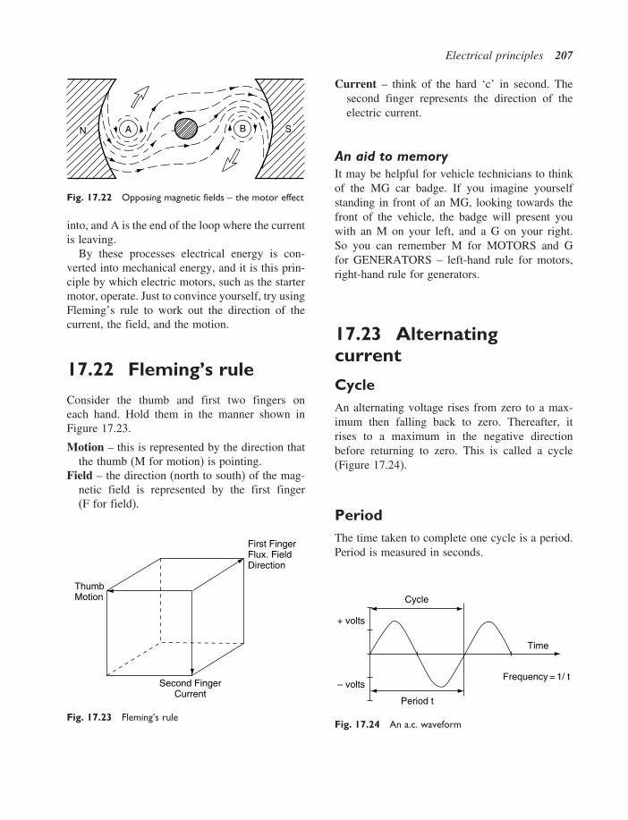
Electrical principles 207
N SA B
Fig. 17.22 Opposing magnetic fields – the motor effect
into, and A is the end of the loop where the currentis leaving.
By these processes electrical energy is con-verted into mechanical energy, and it is this prin-ciple by which electric motors, such as the startermotor, operate. Just to convince yourself, try usingFleming’s rule to work out the direction of thecurrent, the field, and the motion.
17.22 Fleming’s rule
Consider the thumb and first two fingers oneach hand. Hold them in the manner shown inFigure 17.23.
Motion – this is represented by the direction thatthe thumb (M for motion) is pointing.
Field – the direction (north to south) of the mag-netic field is represented by the first finger(F for field).
First FingerFlux. FieldDirection
Second FingerCurrent
ThumbMotion
Fig. 17.23 Fleming’s rule
Current – think of the hard ‘c’ in second. Thesecond finger represents the direction of theelectric current.
An aid to memoryIt may be helpful for vehicle technicians to thinkof the MG car badge. If you imagine yourselfstanding in front of an MG, looking towards thefront of the vehicle, the badge will present youwith an M on your left, and a G on your right.So you can remember M for MOTORS and Gfor GENERATORS – left-hand rule for motors,right-hand rule for generators.
17.23 Alternatingcurrent
CycleAn alternating voltage rises from zero to a max-imum then falling back to zero. Thereafter, itrises to a maximum in the negative directionbefore returning to zero. This is called a cycle(Figure 17.24).
PeriodThe time taken to complete one cycle is a period.Period is measured in seconds.
Cycle
Period t
Time
Frequency = 1/ t– volts
+ volts
Fig. 17.24 An a.c. waveform

208 Automotive science and mathematics
FrequencyFrequency is the number of cycles in one secondand is measured in hertz (Hz). 1 Hz = one cycleper second.
17.24 Applications ofalternating current
In a vehicle alternator (Figure 17.25) the mag-net is the rotating member and the coil of wireis the stationary part in which the electricalenergy to recharge the battery and operate electri-cal/electronic systems is generated. The magneticrotor is driven from the crankshaft pulley and thestationary part – the stator, which contains thecoils – is attached to the alternator case.
N
S
Coil Stator
Rotor
Fig. 17.25 The vehicle alternator
17.25 Transformer
A simple transformer consists of two coils of wirethat are wound round the limbs of an iron core,as shown in Figure 17.26. One coil is the primarywinding and the other is the secondary winding.
Primary
a.cIn
Secondary
Highera.c Out
Iron core
Fig. 17.26 Principle of the transformer
The iron core concentrates the magnetic fieldthat is created by current in the primary wind-ing. The moving lines of magnetic force that arecreated by the alternating current in the primarywinding cut across the coils in the secondary wind-ing and this creates a current in the secondarywinding. The change in voltage that is created bythe transformer depends on the number of turns inthe coils. For example, if there are 10 turns of coilon the primary winding and 50 on the secondary,the secondary voltage will be 5 times the primaryvoltage. This relationship is known as the turnsratio of the transformer.
17.26 Lenz’s law
In an inductive circuit such as that of the solenoid,there is a reaction to the switching off of thecurrent that creates the magnetic field. As themagnetic field dies away, a current is producedthat operates in the opposite direction to the mag-netising current. This effect is known as Lenz’slaw, after the physicist who first explained thephenomenon in the 1830s.
Lenz’s law states:
The direction of the induced emf is alwayssuch that it tends to set up a current oppos-ing the change responsible for inducingthat emf.

Electrical principles 209
17.27 Inductance
Any circuit in which a change of current isaccompanied by a change of magnetic flux, andtherefore by an induced emf, is said to possessinductance. The unit of inductance is the henry(H), named after the American scientist, JosephHenry (1797–1878). A circuit has an inductanceof L = 1 henry (1 H) if an emf of 1 volt is inducedin the circuit when the current changes at a rateof 1 ampere per second. The symbol L is used todenote inductance.
17.28 Back emf
The emf that is created when a device such as arelay is switched off is known as the back emf.
emf = L × rate of increase, or decrease,
of current
= L × I2 − I1
t
where I2 − I1 change of current, and t = time inseconds.
The back emf can be quite a high voltage andin circuits where this is likely to be a problem,special measures are incorporated to minimise the
effect; an example is the surge protection diode inan alternator.
17.29 Inductivereactance
Figure 17.27(a) shows that when the switch is on,the rising current causes the coil (inductor) to pro-duce a current that opposes the battery current. InFigure 17.27(b), the switch is off and the batterycurrent is falling. The current from the inductorkeeps a current flowing in the direction of the orig-inal battery current. In an a.c. circuit, this effectgives rise to inductive reactance, which has thesame effect as resistance. Inductive reactance ismeasured in ohms.
Inductive reactance Xl = 2�f L
where f = frequency, L = inductance in henries.
17.30 Time constant foran inductive circuit
Figure 17.27(c) shows how the current grows fromzero to its maximum value when the switch is
Switch On
(a) (b) (c)
R
L
Switch Off
R
L
Max Current
Cur
rent
Time
Max Current23
Fig. 17.27 Inductive effects

210 Automotive science and mathematics
on. The time taken for the current to reach itsmaximum value is known as the time constant.
The time constant T = LR
seconds
L = inductance in henries, R = resistance in ohms.
Example 17.5A circuit contains a coil having an inductance of2 H is connected in series with a resistance of 4 �.Calculate the time constant for the circuit.
SolutionTime constant T = L
R= 2
4= 0�5 s
17.31 Capacitors
A capacitor is a device that acts as a temporarystore of electricity. In its simplest form a capacitorconsists of two parallel metal plates that are sepa-rated by a material called a dielectric. The externalleads are connected to the two metal plates asshown in Figure 17.28.
When a voltage is applied to the capacitor, elec-trons are stored on one plate and removed fromthe other, in equal quantities. The action sets upa potential difference which remains there whenthe external voltage is removed. The ability of a
capacitor to store electricity is called its capaci-tance. Capacitance is measured in farads – afterMichael Faraday, who worked in London in thenineteenth century.
CapacitanceCapacitance is determined by the properties of thedielectric and the dimensions of the metal plates.It is calculated from the formula
C = �o�rAd
farads
The terms �o �r are properties of dielectric andthey are called permittivity. A is the area of theplates and d is the distance between them.
Capacitance in a circuitFigure 17.29(a) shows a circuit that can be usedto examine the charging of a capacitor. Whenthe switch is closed the capacitor is discharged.When the switch is opened, the capacitor willrecharge. The voltmeter is observed while the timeis recorded. The result is plotted and a graph of thetype shown in Figure 17.29(b) is produced. Thisgraph shows how the capacitor voltage changeswith time. The time taken for the capacitor to
Metal Plates
LeadLead
Dielectric
– – ––
Electrons–
+
+
+
++
+
+
+–
––
–
–
–– –
Electrons
P.D. (Voltage) Applied to PlatesElectrons Stored on One Plate Equal
Number of Electrons Leave the Other Plate
Fig. 17.28 A simple capacitor

Electrical principles 211
C
V
R
(a)
(b)
T = RC Time – Seconds
MaxVolts
Max23
Fig. 17.29 Charging a capacitor
reach two thirds of the supply voltage is knownas the time constant for the circuit.
Time constant T = R ×C
where R = resistance in ohms, C = capacitancein farads.
Capacitance values are normally given in mil-lionths of a farad, known as microfarads, anddenoted by the symbol �F.
Example 17.6A circuit of the type shown in Figure 17.29(a)has a resistance of 10 000 � and a capacitanceof 10 000 �F. Calculate the time constant for thecircuit.
SolutionTime constant T = C × R = 0�01 × 10 000 =100 seconds.
17.32 Capacitors incircuits
Contact breaker ignition circuitIn the contact breaker-type ignition system acapacitor is placed in parallel with the contactbreaker (Figure 17.30). When the contact pointsopen, a self-induced high-voltage electric chargeattempts to arc across the points. The capacitorovercomes this problem by storing the electriccharge until the points gap is large enough to pre-vent arcing.
ContactPoints
C
Ignition Coil
Fig. 17.30 Capacitor in contact breaker ignition circuit
Capacitive dischargeignition systemIn the capacitive discharge ignition system thecapacitor stores electrical energy until a sparkis required (Figure 17.31). To generate a spark,an electronic circuit releases the energy from the

212 Automotive science and mathematics
C
ControlElectronics
Fig. 17.31 A capacitive discharge ignition system
capacitor into the ignition coil circuit, a high-voltage spark thereby being produced at the spark-ing plug.
Capacitors in parallel and seriesParallel capacitorsFigure 17.32(a) shows two capacitors connectedin parallel. The total capacitance provided by thetwo capacitors = C = C1 +C2.
C1 C2
(a) Parallel Capacitors
C1
C2
(b) Series Capacitors
Fig. 17.32 Capacitors in circuits
Series capacitorsFigure 17.32(b) shows the two capacitors con-nected in series. In this case, the total capacitanceC is given by the equation C = C1 C2/C1 +C2.
Example 17.7Two capacitors, one with a capacitance of 8 �Fand the other with a capacitance of 4 �F are con-nected (a) in parallel, (b) in series. Determine thetotal capacitance in each case.
Solution(a) Total capacitance C = 8+4 = 12 �F
(b) Total capacitance C = 8×48+4
= 3212
= 2�67 �F
ImpedanceFigure 17.33 shows a circuit that contains a resis-tor, an inductor (coil) and a capacitor. The com-bined effect of these three devices in an a.c.circuit produces an effect known as impedance.Impedance acts like a resistance and it is measuredin ohms.
R L C
Ω Ω2πFL Ω
2πFC1
G
Fig. 17.33 Impedance
17.33 Summary offormulae
Ohm’s law: V = IR
Power = VI watts
Series resistance, R = R1+R2+· · ·

Electrical principles 213
Parallel resistance,1R
= 1R
+ 1R1
or R = R1 R2
R1 +R2
Capacitors in parallel, C = C1+C2
Time constant for inductive circuit t = R × C
Capacitance C = �o�r Ad
farads
Time constant for inductive circuit t = the time
constant T = LR
seconds
Lenz’s law: The direction of the induced emf isalways such that it tends to set up a current oppos-ing the change responsible for inducing that emf.
17.34 Exercises
17.1 In the circuit shown in Figure 17.34, whatis the total series resistance?(a) 1.33 �(b) 6 �(c) 8 �(d) 2 �
4 Ω 2 Ω
V
A
12 V
Fig. 17.34
17.2 In the circuit in Figure 17.34, what is thecurrent at the ammeter?(a) 6 A(b) 8 A(c) 2 A(d) 1 A
17.3 In the circuit of Figure 17.34, what is thevoltage drop across the 4 � resistor?(a) 8 V(b) 12 V(c) 3 V(d) 1 V
17.4 In the circuit of Figure 17.35, what is theequivalent series resistance of the two resis-tors in parallel?(a) 8 �(b) 1.5 �(c) 3 �(d) 12 �
17.5 In Figure 17.35, what is the current at theammeter?(a) 1 A(b) 1.5 A(c) 8 A(d) 24 A
17.6 In Figure 17.35, what is the current in the2 � resistor?(a) 4 A(b) 6 A(c) 1.5 A(d) 1 A
2 Ω
6 Ω A
12 V
Fig. 17.35
17.7 In the circuit in Figure 17.36, what is theequivalent series resistance of the threeresistors?(a) 16 �(b) 12.4 �(c) 0.55 �(d) 4 �

214 Automotive science and mathematics
17.8 In the circuit of Figure 17.36, what is thetotal current flow at the ammeter?(a) 48 A(b) 3 A(c) 0.97 A(d) 5 A
17.9 In the circuit in Figure 17.36, what is thevoltage drop across the 2.4 � resistor?(a) 9.6 V(b) 3 V(c) 7.2 V(d) 4.8 V
2 Ω
8 Ω
2.4 Ω
A
V
12 V
Fig. 17.36
17.10 What is the total capacitance of thetwo capacitors in parallel as shown inFigure 17.37?(a) 15 000 �F(b) 1�5 �F(c) 250 �F(d) 0�67 �F
C1 = 100 μF
C2 = 150 μF
Fig. 17.37
17.11 Does the capacitor in parallel with the igni-tion points of a coil ignition system, asshown in Figure 17.38:(a) prevent arcing across the points?(b) act as a suppressor to reduce radio
interference?(c) reduce erosion at the spark plug con-
tacts?(d) prevent current overload in the coil pri-
mary circuit?
CContactBreakerPoints
IgnitionCoil Primary
Fig. 17.38
17.12 The time constant for a capacitor in a circuitthat contains resistance is the time that ittakes to charge the capacitor to(a) 6% of the charging voltage(b) 67% of the charging voltage(c) 33% of the charging voltage(d) the full charging voltage
17.13 Is Fleming’s right hand rule useful forworking out the direction of current flow in(a) the armature winding of a starter
motor?(b) the armature winding of a generator?(c) the winding of a non-inductive resistor?(d) a solenoid?
17.14 Impedance in an a.c. circuit is the totalopposition to current flow that the circuitcauses. Is impedance measured in(a) watts?(b) amperes?(c) ohms?(d) coulombs?

Electrical principles 215
17.15 In a metal conductor the flow of current iscaused by the drift of free electrons. Is thefree electrons flow(a) from the positive to the negative elec-
trode?(b) from a lower electrical potential to a
higher electrical potential?(c) from the positive to the negative termi-
nal of the battery?(d) from high electrical potential to low
electrical potential?17.16 A 12-volt electric motor takes a current of
20 A. Is the power of the motor(a) 1.67 kW(b) 0.3 kW(c) 240 W(d) 32 W
17.17 Does Lenz’s law state that(a) the direction of an induced emf is
always such that it tends to set up a
current opposing the change responsi-ble for inducing the emf?
(b) V = IR?(c) t = RC?(d) the back emf is directly proportional to
the capacitance?17.18 Are electrical conductors materials
(a) in which free electrons can be made tomove?
(b) that have a high specific resistance?(c) that do not heat up when current
flows?(d) that are always physically hard?
17.19 Does a circuit that has a resistance of10 000 � and a capacitance of 10 000 �Fhave a time constant of(a) 10 seconds?(b) 0.1 seconds?(c) 100 seconds?(d) 1000 seconds?

18Electronic principles
18.1 Introduction
Microprocessors are small computers which finduse in many vehicle systems such as engine man-agement, anti-lock braking, and traction control(Figure 18.1).
In order to function, the microprocessorrequires inputs from sensors. These inputs are usedto make decisions which, in turn, are used to makeoutputs that enable the operation of various actua-tors. Many of these sensors and actuators operateon electronic principles.
Inputs
Speed Sensor
Air Flow Sensor
TemperatureSensor
Crystal
Clock
CentralProcessing
Unit(CPU)
Memory
ProgramMicroprocessor
Outputs
Fuel Injection
EGRValve
Fig. 18.1 Microprocessor-controlled vehicle systems
The subject matter in this chapter is designed toprovide an insight into basic electronic principles.
18.2 Semiconductors
Materials such as copper have many free electronsin their outer shells. These free electrons can bemade to flow in a circuit under the influence ofan applied voltage, and they are good conductors.Semiconductor materials such as pure silicon havefew electrons in their outer shells, which makes

Electronic principles 217
them poor conductors of electricity. The conduc-tivity of pure silicon is improved by diffusingimpurities into it under high temperature. Impuri-ties that are often used for this purpose are boronand phosphorus, and they are called dopants.
Effect of dopantsWhen boron is diffused into silicon the result-ing material is known as a p-type semiconduc-tor. When phosphorus is diffused into silicon it isknown as an n-type semiconductor.
Electrons and holesPhosphorus doping gives surplus electrons tothe material. These surplus electrons are mobile.Boron doping leads to atoms with insufficientelectrons that can be thought of as holes. P-typesemi-conductors have holes whereasN-type semi-conductors have surplus electrons. When a p.d.(voltage) is applied, electrons drift from − to +,and holes drift from + to −.
18.3 The p–n junction
When a piece of p-type semiconductor is joinedto a piece of n-type semiconductor, a junction isformed (Figure 18.2). At the junction an exchange
+++
+
+++
––– –
–––
–
–
–
–
3 4
NP
251
1. Holes2. Electrons3. Negative Charges4. Positive Charges5. Depletion Layer
Fig. 18.2 A p–n junction
of electrons and holes takes place until an elec-trical p.d. which opposes further diffusion isproduced between the two sides of the junction.The region where this barrier exists is known asthe depletion layer and it acts like a capacitorthat holds an electric charge.
18.4 Bias
When a p–n junction is placed in a circuit, as shownin Figure 18.3(a), the battery provides a potentialdifference across the depletion layer. This over-comes the barrier effect and allows electrons toflow through the p–n junction (diode) and the lampwill illuminate. This is known as forward bias.
(a) (b)
P N
LampOn
P N
LampOff
Fig. 18.3 Forward and reverse bias
When the battery connections are reversed, asshown in Figure 18.3(b), a reverse bias is appliedat the p–n junction. This reinforces the barriereffect at the depletion layer and prevents a flowof current through the circuit. The result is thatthe lamp will not illuminate. The voltage requiredto overcome the barrier potential is known as theknee voltage and it is approximately 0.7 V for asilicon diode.
A junction diode, or just diode, is an effectiveone-way valve in an electronic circuit.
18.5 Behaviour of a p–njunction diode
Figure 18.4(a) shows a circuit in which the resis-tor can be changed to vary the current in thecircuit and hence the voltage across the diode.

218 Automotive science and mathematics
(a) (b)
R
V
A
SiliconDiode
0
Current I
0.7 v Voltage V
Fig. 18.4 Current–voltage in forward biased diode
A series of readings of current and voltage for var-ious resistance values will produce a graph of theform shown in Figure 18.4(b). This graph showsthat there is very little current below 0.7 V but assoon as the voltage reaches 0.7 V the current risesrapidly.
18.6 Diode protectionresistor
If the current in a diode is too large, the heatingeffect will destroy the diode properties. To preventthis happening a resistor is placed in series withthe diode and this restricts the current through thediode to a safe level. The diode current may becalculated from
I = Vs−VdR
where R = resistance in ohms, Vs = supply volt-age, Vd = diode voltage.
Example 18.1In the circuit shown in Figure 18.4(a), the resistorvalue = 1 k�, the supply voltage = 12 V, andthe silicon diode voltage = 0.7 V. Calculate thecurrent through the diode.
SolutionDiode current I = 12−0�7
1000= 0�0113 A = 11�3 mA
18.7 Negativetemperature coefficientof resistance –semiconductor
When the temperature of a semiconductor isincreased, thermal activity causes an increasein electrons and holes. These actions increasethe conductivity of the semiconductor. (SeeFigure 18.5.)
0 10 20 30 40 50 60 70 80
50
100
Res
itanc
e kΩ
Temperature °C
Fig. 18.5 Negative temperature coefficient
18.8 The Zener diode
The Zener diode is a p–n junction diode thatis designed to break down at a specified volt-age (Figure 18.6). The breakdown mechanism isnon-destructive provided that the current is lim-ited to prevent overheating. The voltage at whichbreakdown occurs and current flows in the reversedirection is known as the Zener voltage. Oncecurrent flows in the reverse direction the voltagedrop across the Zener diode remains constant atthe Zener voltage. Zener voltages normally fall inthe range 3 V to 20 V. The actual figure is chosenat the design stage, typical values being 5.6 V and6.8 V. Two common uses of the Zener diode inautomotive practice are voltage surge protectionin an alternator circuit and voltage stabilisation ininstrument circuits.

Electronic principles 219
Fuel ReceiverGauge
Fuel Sender Gauge(Sliding Resistor)
R
E
HI
F
C
ZD
HeatWire
Water TemperatureReceiver Gauge
Water TemperatureSender Gauge(Thermistor)
Fig. 18.6 The Zener diode as a voltage regulator
18.9 Light emittingdiode (LED)
When electrons have been moved into a largerorbit they may fall back to their original energylevel. When this happens, the electrons give upenergy in the form of heat, light, and other formsof radiation. The LED utilises this effect, the vari-ous types found emitting light of different colours.When elements such as gallium, arsenic and phos-phorus are used, colours such as red, green andblue are produced.
Voltage and current in an LEDMost LEDs have a voltage drop of 1.5 to 2.5 voltswith currents of 10 to 40 mA. In order to limit thecurrent, a resistor is placed in series with an LED,as shown in Figure 18.7.
Example 18.2The voltage drop across the LED in Figure 18.7 is2 V and the maximum permitted current is 20 mA.
The voltage drop across the resistor is �9−2� =7 V
Using Ohm’s law, R = VI
= 70�02
= 350 �.
R
9 V
LED Current 20 mALED Voltage 2 V
Fig. 18.7 The current-limiting resistor – LED
18.10 Photodiode
When radiation in the form of light falls on ap–n junction diode, some electrons are caused tomove thus creating an electric current. The greaterthe intensity of the light falling on the diode, thegreater the current. This makes photodiodes suit-able for use in a range of automotive systems suchas security alarms and automatic light operation.
18.11 Bipolar transistors
Bipolar transistors use both positively and neg-atively charged carriers. This form of transis-tor basically comprises two p–n junction diodesplaced back to back to give either a p–n–p type,

220 Automotive science and mathematics
p
c en n
b
LampOff
p
ec
n nb
LampBegins to Light
(a) (b) (c)
p
ec
n nb
LampFull On
Fig. 18.8 A simple transistor
or an n–p–n type. In both cases the transistor hasthree main parts, these being the collector, theemitter and the base, as shown in Figure 18.8(a),(b), and (c) respectively.
Basic operation of transistorFigure 18.8(a) shows an n–p–n transistor in a cir-cuit that includes a battery and a lamp. There isno connection to the base – the transistor is notbiased. Virtually no current flows in the circuitand the lamp will not illuminate.
In Figure 18.8(b) a voltage source is applied tothe base of the transistor and this causes electronsto enter the base from the emitter. The free elec-trons can flow in either of two directions; i.e. theycan flow either into the base or into the collector,which is where most of them go. In this phase thelamp begins to light.
Once free electrons are in the collector theybecome influenced by the collector voltage andcurrent flows freely through the main circuit toilluminate the lamp. This phase is shown inFigure 18.8(c).
This switching action takes place at very highspeed, which makes transistors suitable for manyfunctions in electronic and computing devices.
Current gain in transistorUnder normal operating conditions the collectorcurrent Ic is much larger than the base current Ib.
The ratio Ic/ Ib is called the gain and is denotedby the symbol �.
� = IcIb
Values of current gain vary according to the typeof transistor being used. Low-power transistorshave current gains of approximately 100 to 300,high-power transistors less than 100.
Example 18.3A certain transistor has a current gain of 120.Determine the collector current Ic when the basecurrent Ib = 0�1 mA.
Solution
� = IcIb
Ic = �× Ib
Ic = 120×0�1
= 12 mA
Current flow in transistorsFigure 18.9 shows the path of current flow intransistors. It is useful to study this when workingout how circuits operate.

Electronic principles 221
R
+ Pos _ Neg
b
c
e
b
c
e
npn Common Emitter
(a) (b)
pnp Common Emitter
Ic Ic
Ib
IbIb
Ie = Ib + Ic
Fig. 18.9 Current flow in transistors
18.12 Transistor circuitused in automotiveapplications
Voltage amplifierSome devices such as sensors in vehicle systemsproduce weak electrical outputs. These weak out-puts are amplified (voltage is increased) to makethem suitable for use in operating a vehicle sys-tem. The circuit shown in Figure 18.10 shows asimple voltage amplifier circuit.
Rb
C1
Low VoltageHigh Voltage
C2
Rc
Fig. 18.10 Voltage amplifier
Darlington pairA Darlington pair is a circuit that contains twotransistors, as shown in Figure 18.11. The effect is
0.0015 mA
0.3 mA60 mA
β = 200T1
T2
β = 200
Fig. 18.11 Darlington pair
that the circuit behaves as a single transistor with avery high current gain. The collector current fromT1 is fed to the base of T2.
In the example shown , the transistors each havea current gain of � = 200. This gives a collectorcurrent at T1 of 0.3 mA, which becomes the basecurrent of T2 and the resulting collector current atT2 is 200×0�3 = 60 mA.
A Darlington pair is often used to provide thecurrent for the primary winding of an ignition coil.
Heat sinkSemiconductor devices are adversely affectedby temperatures outside their designed operatingrange. In low-power devices the heat is normallydissipated through the structure of the circuit andits surroundings. High-power devices such as the

222 Automotive science and mathematics
DiodeMetallic
Heat Sink
Fig. 18.12 A diode and its heat sink
Darlington pair are mounted on a metal heat sinkthat conducts the heat away from them.
18.13 Filter circuits
Electrical filters are used to prevent certain alter-nating currents from reaching parts of a circuitwhere they affect performance. The filter circuitsshown in Figure 18.13 operate on the principlethat at certain frequencies a capacitor will becomea conductor of electric current.
The low-pass filter, shown in Figure 18.13(a), isdesigned to pass low frequencies from the input tothe output. At higher frequencies the capacitor iseffectively short circuited and the high frequencycurrent bypasses the output terminals.
In the high-pass filter, shown in Figure 18.13(b),the low frequencies are effectively blocked. Ata certain frequency the capacitor will become a
R
(a) (b)
OutCIn R
C
OutIn
Fig. 18.13 Low-pass and high-pass filters
conductor and the higher-frequency current willpass to the output terminals.
Voltage dividerVoltage dividers are used in circuits where apotential difference (voltage) that is a fraction ofan applied emf, is required (Figure 18.14).
I
R1
R2
V2
V1
Vs
Fig. 18.14 The voltage divider
As R1 and R2 are in series, the same current Iflows through both of them.
The resistance of the circuit = R1 +R2
The supply voltage = Vs
The current I = VsR1 +R2
= V1
R1
From this� V1 = R1VsR1 +R2
(18.1)
Similarly� V2 = R2VsR1 +R2
(18.2)
Example 18.4Figure 18.15 shows a voltage divider circuit.Determine the value of V1 and V2.
SolutionUsing Equation (18.1)
V1 = 1×91+8
= 1 volt

Electronic principles 223
R1V1
V2
Vs
R2
1 kΩ
8 kΩ
9 V
Fig. 18.15 Example – voltage divider
Using Equation (18.2)
V2 = 8×91+8
= 8 volts
18.14 Integrated circuits
Large numbers of capacitors, transistors anddiodes can be made on a small piece of silicon.These components are then connected to formcomplicated circuits. These circuits are known asintegrated circuits (ICs) and the small piece ofsilicon is referred to as a ‘chip’.
18.15 Sensors andactuators
A sensor is a device that detects some aspect ofvehicle performance and converts it into an elec-trical signal that is fed to the control computer foruse in controlling factors such as engine fuellingand ignition timing. A sensor may be classed asone of two types:
1. Active sensors – these produce electricitythat represents the variable that they aredetecting. They are often electromagnetic or,as in the case of zirconia oxygen sensors,electrochemical.
2. Passive sensors – they receive a supply ofelectricity and process it so that the control unitdetects changes. In the case of the negativetemperature coefficient sensor used to detectcoolant temperature, the changes in resistanceproduce a varying sensor voltage that repre-sents coolant temperature.
Typical examples of sensors are:
• air flow;• exhaust gas oxygen;• engine speed;• crank position;• throttle position;• engine coolant temperature.
An actuator is a device that is controlled by com-mands that are outputs from the control computer,typical examples being;
• fuel injector;• anti-lock braking modulator;• exhaust gas recirculation valve.
The simple moving flap type of air flow sensorshown in Figure 18.16 makes use of a potentialdivider that interprets air flow as a voltage. Thewiper of the potential divider is fixed to the spindleof the sensor. When the flap moves in responseto changes in air flow, the wiper moves along theresistance strip. The voltage Vs that is transmittedto the control computer is an exact representationof air flow.
The petrol injector shown in Figure 18.17 is anelectromagnetic actuator that operates in a waythat is similar to the action of a solenoid. Currentto the injector is supplied via a relay and the con-trol computer switches the power transistor on,so that the injector is operated. The duration ofthe injection period determines the amount of fuelthat is injected into the engine. The duration ofthe injection period (and thus the amount of fuelinjected) is determined by the computer program,which makes use of the input from the air flowsensor and from other sensors for throttle position,engine speed and engine coolant temperature, forexample.

224 Automotive science and mathematics
Potential Divider
x
A
Air Supply Signal
C B
Vs
Vc
Constant Voltage toAir Flow Sensor
Control Computer
(a)
Air toEngine
Air fromAir Filter
Spindle
1
2
431. Spiral Spring 2. Compensating Flap3. Metering Flap 4. Idling Air Passage
(b)
VsVc
Vs = Output VoltageVc = Constant Voltage Supply
Spindle
Resistance Strip
o
The Voltage vs Represents Air Flow
(c)
Fig. 18.16 Air flow sensor
SolenoidWinding
NozzleValve
(a) (b)
Current from Ignition Switch
Power Transistor
Base CurrentControlledby Computer
Earth
Fig. 18.17 Petrol injector

Electronic principles 225
18.16 Control unit(computer) inputs andoutputs
Inputs to the control unit are often of varyingvoltage (analogue) form. These inputs are receivedat an interface that contains an analogue-to-digital(A/D) converter. The A/D converter changes theinput voltage to a binary (digital) code that is usedby the central processing unit (cpu) to enable thecontrol unit to deliver output signals. The outputsare of varied forms, for example an instruction tooperate the fuel injectors for a set period in eachpower stroke of the engine.
18.17 Logic gates
Transistor switches can be built into small circuitsto make devices called logic gates. These gatesoperate on digital (binary) principles.
The RTL NOR gateFigure 18.18 shows how a ‘logic’ gate is built upfrom an arrangement of resistors and a transistor(RTL = resistor transistor logic). There are threeinputs: A, B and C. If one or more of these inputsis high (logic 1), the output will be low (logic 0).
Rb Rc
Vcc
Rb
Rb
A
B
C
5 V
Output = A + B + C
Fig. 18.18 RTL NOR gate
The output is shown as A+B+C with a line, orbar, over the top; the + sign means OR. Thus theA+B+C with the line above means ‘not A or Bor C’ (NOR: NOT OR).
The base resistors Rb have a value that ensuresthat the base current, even when only one input ishigh (logic 1), will drive the transistor into satu-ration to make the output low (logic 0).
Truth tablesLogic circuits operate on the basis of Booleanlogic, and terms such as NOT, NOR andNAND derive from Boolean algebra. This neednot concern us here, but it is necessary toknow that the input–output behaviour of logicdevices is expressed in the form of a ‘truthtable’.
The truth table for the NOR gate is given inFigure 18.19.
In computing and control systems, a systemknown as TTL (transistor to transistor logic) isoften used. In TTL logic 0 is a voltage between0 and 0.8 volts. Logic 1 is a voltage between 2.0and 5.0 volts.
In the NOR truth table, when the inputs A andB are both 0 the gate output, C, is 1. The otherthree input combinations each gives an output ofC = 1.
A range of other commonly used logic gatesand their truth tables is given in Figure 18.20.
A
B
C
Inputs Outputs
A
0011
B
0101
C
1000
Fig. 18.19 NOR gate symbol and truth table

226 Automotive science and mathematics
A
BX
A
BX
A
BX
A
BX
A X A X
A
BX
A
BX
A
BX&
A
BX&
Type of Logic Gate
USA Symbol UK Symbol Truth Table
AND
OR
(NOT AND)NAND
NOTInverter
(NOT OR)NOR
OutputsInputs
A B
0 00 11 01 1
X
0001
Inputs
A B
0 00 11 01 1
0001
X
OutputsInputs
A B
0 00 11 01 1
0111
X
OutputsInputs
A B
0 00 11 01 1
1110
X
OutputsInputs
A B
0 00 11 01 1
1000
X
OutputsInputs
A
01
10
Fig. 18.20 A table of logic gates and symbols

Electronic principles 227
18.18 Bits, bytesand baud
Each 0 and 1 in a binary code is known as a bit,and 8 bits make one byte. Because large numbersof bits are used in computer processes, larger unitsare used. Examples of these larger units are:
a kilobyte, 1 kbyte = 210 = 1024 bytesa megabyte, 1 Mbyte = 220 = 1 048 576 bytes
The rate at which data in the form of binary bitsis moved around a computer system is known asthe baud rate; a rate of data transfer of one bit persecond is = 1 baud. The term baud derives fromJean Baudot, the French technologist. In vehiclesystems such as traction control data transfer ratesof 250 kbaud to Mbaud are used.
18.19 Summary offormulae
Forward voltage of silicon diode = 0.7 V (approx.)
The diode current may be calculated from
I = Vs−VdR
where R = resistance in ohms, Vs = supply volt-age, Vd = diode voltage
The ratioIc
Ib
is called the gain and it is denoted
by the symbol �
� = Ic
Ib
18.20 Exercises
18.1 Are electronic components such as alter-nator diodes mounted on a metalheat sink(a) to avoid damage by vibration?(b) to conduct surplus electric current to
earth?
(c) to allow heat to be conducted awayfrom the diode to prevent damage?
(d) to improve the electrical conductivityof the circuit?
18.2 A certain transistor has a current gain of100. Is the collector current Ic when thebase current Ib = 0�1 mA(a) 10 A(b) 10 mA(c) 99 mA(d) 1 A
18.3 Do active sensors(a) process an electrical supply?(b) produce electricity that represents the
variable they are detecting?18.4 Do electrical filters
(a) filter out a.c. frequencies that mayinterfere with the operation of an elec-tronic system?
(b) only work in a d.c. circuit?(c) only find use in radio circuits?(d) never find use in automotive systems?
18.5 State the reason for using an analogue-to-digital converter on computer-controlledsystems.
18.6 In an OR logic gate, is(a) the output 1 when both inputs are 0?(b) the output zero when both inputs are 1?(c) the output 1 when any of the inputs
are 1?(d) the output 0 when any input is 1?
18.7 Do traction control systems have a datatransfer rate of(a) 10 bits per second?(b) 1000 bits per second?(c) 10 000 bits per second?(d) 250 kbaud to 1 Mbaud?
18.8 In a computer-controlled automotive sys-tem, do actuators(a) operate devices under the instructions
of the control computer?(b) sense engine temperature and convert
it into a voltage?(c) convert analogue signals to digital
ones?(d) store fault codes?

228 Automotive science and mathematics
18.9 Is the part of the computer that controls themovement of data(a) the A/D interface?(b) the clock?(c) the baud rate?(d) the speed of the vehicle?
18.10 Is a petrol injector(a) a sensor?(b) an actuator that operates on the princi-
ple of a solenoid?(c) operated from the cam shaft?(d) a variable capacitance oscillator?
18.11 Are Zener diodes used(a) to convert a.c. to d.c.?(b) to provide surge protection?
(c) as an element in a liquid crystal dis-play?
(d) to block all current flow in the reversedirection?
18.12 In order to limit the current flow throughan LED, is(a) a resistor placed in parallel with the
LED?(b) the supply voltage limited?(c) a resistor placed in series with the
LED?(d) it essential to increase the dopant level?

Answers to self-assessmentquestions
Chapter 1
1.1 0.50 mm1.2 15.12 mm1.3 Total gap =0�35 mm. This is to be reduced
to 0.15 mm. Total space to be taken up =0�20 mm. Each thrust washer must be0.10 mm thicker
1.4 Offset =2 mm1.5 X = 0�9 mm1.6 X = 4�2 mm1.7 Overall gear ratio =1�531×4�3 = 6�58 � 11.8 (a) 3, (b) 2, (c) 144, (d) 78.551.9 16.15 km/l
1.10 Swept volume = CSA × L × number ofcylindersSwept volume = 55�6×9×4 cm3
= 2000�00 cm3 = 2�00 litres1.11 (a) 6.00, (b) 14.12, (c) 0.691.12 (a) 37.87, (b) 48.70, (c) 39 487 000,
(d) 0.00771.13 £9.92 p1.14 Total cost of labour before VAT = 6�33 ×
42 = £265�86Total cost before VAT = £265�86 +£102�58 = £368�44
1.15 Fuel used = 186 ÷ 10�36 = 17�95 litres,correct to two decimal places
1.16 Weight of fuel =220 × 0�83 = 182�6 kgTotal weight of tank and fuel =30+182�6 =212�60 kg
1.17 (a) a6, (b) x, (c) 56, (d) t6, (e) 101.18 (a) 3, (b) 9, (c) 81, (d) 51.19 (a) 0.125, (b) 0.125, (c) 2, (d) 0.2001.20 (a) 3, (b) 9, (c) 19, (d) 81.21 (a) 13, (b) 18, (c) 71.22 1/3 + 1/ 2 + 5/8 + 1/ 4 + 3/8 =
8+12+15+6+924
= 5024
= 21/12 litres
The lowest common denominator 2, 3, 4,8 = 24
1.23 (4+3+1)+(1/2+3/4 + 7/8� = 8+ 4+6+78
=8+21/ 8 =10
1.24 (a) 3/10, (b) 1/8, (c) 3/8, (d) 5/8
1.25 (a)15+10+24−5
30= 44
30= 1
1430
(b) 213
− 114
+ 58
= 7/3 − 5/4 + 5/8
= 56−30+1524
= 4124
= 117/24
(c)1
32− 1
16+ 3
8+9
= 9+ 1−2+1232
= 9 11/32

230 Automotive science and mathematics
1.26 (a)19
(b)45
× 58
÷ 78
× 89
= 4×5×8×85×8×7×9
= 4×87×9
= 3263
(c)1
64
1.27 (a)(
13
÷ 14
)
− 16
= 43
− 16
= 8−16
= 76
=
116
(b)(
181
+ 19
)
× 124
= 1081
× 124
= 3081
(c)(
43
÷ 16
)
+ 38
+ 132
= 8 + 38
+ 132
= 8 13/32
1.28 Largest first: 0.21 0.201 0.2001 0.2 0.021
1.29 Smallest first:38
12
45
56
1.30 1101112
1.31 �10×162�+ �2×161�+ �15×160�= 2560+32+15 = 2607
Chapter 2
2.1 (a) Arithmetic mean = 6�22, median = 6(b) Mode = 9(c) 4 and 7
(d) Median = 9+112
= 10
(e) 55 marks2.3 Angle of pie chart for CO = 155�2�
Angle of pie chart for HC+NOx = 170�7�
Angle of pie chart for SO2 = 34�1�
2.4 Angle of pie chart for lack of fuel =98�9degreesAngle of pie chart for electrical problems =142�1 degreesAngle of pie chart for tyre problems = 86�5degreesAngle of pie chart for fuel system faults =32�5 degrees
2.5 Profit = 45−39�50 = £6�50 per hourAngles on pie chart
Technicians’ pay = 76 degreesHeating of premises = 56 degreesAdmin. and other overheads = 184 degreesProfit = 52 degrees
2.10 Number of people working less than 30hours = 26
Chapter 3
Exercises – Section 3.31. 3202. 23. 523.84. 28005. 116. 1437.37. 19.88. 4�22×107
9. 47 10010. 40
Exercises – Section 3.41. 3ab+12ac+6ab−9ac−5bc = 9ab+3ac−5bc2. (a) 18ab−8ac, (b) 14x+21y, (c) 6x+213. 5x−3x+30+8−2x = 38
Exercises – Section 3.5(a) 6+2x+3y +xy, (b) x2 +5x+6,
(c) x2 +x−6, (d) x2 −6x+8
Exercises – Section 3.6(a) 2x�x−2�, (b) �a +2b��x+2�, (c) ax�x+1�
Exercises – Section 3.71. x = 42. y = 33. d = 304. x = 55. x = 46. x = 167. x = 1/ 3
8. x = −9

Answers to self-assessment questions 231
Exercises – Section 3.8
1. x = y − cm
2. L = √�T/4Mn2�
3. d = C�
4. I = VR
5. L = 4V�d2
Exercises – Section 3.103. Graph4. From the graph, piston velocity at 90� =
8�4 m/s.5. The law is P = 1�5 W +1�2
Chapter 4
4.1 720�
4.23000
60×2� = 314�2 rad/s
4.3 36�24′
4.4 Largest acceptable angle 31�10′ +55′
= 32�5′
Smallest acceptable angle = 31�10′ −55′
= 30�15′
4.5 33�55′ −31�10′ = 2�45′
4.6 180� +10+45� = 235�
4.7 15� +20� = 35�
4.8 31�
4.9 (c)4.10 65�
4.11 135�
4.12 12�
4.13 45�
4.14 y = √�1402 − 552� = √
�19600 − 3025� =√16 575 = 128�74 mm
Original distance from centre of gudgeon pinto centre of crank = 140+55 = 195 mmDistance x = 195 − y = 195 − 128�74 =66�26 mm
4.15 1/2 d = √�252 − 202� = √
�625 − 400� =√225 = 15�d = 2×15 = 30 mm
Ans. 4.16. x = √�2002 +1002� =√
50000 = 223�6mm.4.17 1/2d = √
�27�52 −13�752� =√�756�25−189�06� = √
567�19 = 23�82∴ d = 2×23�82 = 47�64 mm
4.18 Distance moved during one revolution of thewheel and tyre = 2�r = 2 ×3�142 ×0�25 =1�571 mDistance moved when wheel makes1000 revolutions=1�571×1000=1571m =1�571 km
4.19 Effective area of valve opening =� ×diameter of valve×valve lift= 3�142×35×12 = 1319�6 mm2
4.20 Distance travelled by vehicle per minute =rev/min of wheel× rolling circumference= 600×� ×0�3×2 = 1131�1 m/min
Speed of vehicle in km/h = 60×1131�11000
=67�87 km/h
4.21 Original area of valve opening = � × 30 ×14 = 1320 mm2
Area after opening up ports and increasingvalve lift = � ×30�5×15 = 1437�5 mm2
Increase in area = 1437�5 − 1320 =117�5 mm2
Percentage increase
= increase in area of valve openingoriginal area of valve opening
= 117�51320
×100 = 8�9%
4.22 Length of arc= �× circumference360� =
25� ×3�142×400 mm360� = 87�3 mm
4.23 (a) 0.669, (b) 0.9976, (c) 0.4848, (d) 0.2588,(e) 0.3947, (e) 0.5000
4.25 23.57 m/s4.26 (a) 17.04, (b) 14, (c) 54.28 (a) x = 4�66 m, (b) x = 138�93 mm,
(c) x = 90�57 mm4.29 (a) � = 53�13�, (b) � = 28�07�, (c) � = 22�62�
4.30 (a) 26�6�, (b) 36�87�, (c) 28�07�, (d) 53�06�

232 Automotive science and mathematics
4.31 (a) x = 7�98 cm, (b) x = 7�46 cm, (c) x =156�25 mm
4.32 � = 73�3�� x = 208�8 mmDistance that piston has moved from
TDC = 260−208�8 = 51�2 mm
Chapter 5
5.1 2250 N5.2 3 N/mm5.3 (a)5.4 Resultant 135 N at 214�12′ to A. The equi-
librant is equal in magnitude but oppositein direction.
5.5 98.8 N. Direction towards at angle of41�41′ to force A.
5.6 (a) 7 mm, (b) 200 N5.7 Horizontal component = 5×cos 40� = 5×
0�766 = 3�83 kN5.8 Jib = 5�25 T, tie = 3�05 T5.9 Side thrust F = 1180 N
5.10 Force A = 13 N, force B = 48 N5.11 Force Q = 1080 N, force P = 1340 N5.12 Pressure on piston crown = 25 bar
15.13 (c)15.14 (b)
Chapter 6
6.1 0.00221 mm6.2 (b) 3.33 MN/m2, (c) 0�007 mm6.3 49�02 MN/m2
6.4 Angle of twist = 0.012 degrees6.5 (a) 28�4 MN/m2, (b) 26�7 MN/m2
6.6 24�54 MN/m2
6.7 fs = 595 Mpa6.8 Maximum permissible torque = 157.2 Nm6.9 Tensile force = 10.6 kN
6.10 164�7 GN/m2
6.11 19�22 MN/m2
6.12 (a) 1500 N, (b) 19�1 MN/m2
6.13 88 kW
Chapter 7
7.1 (b) 33.3 N7.2 Rr = 0�955 tonne; 1�8−0�955 = 0�845 tonne7.3 x = 1�527 m7.4 R2 = 3�8 T, R1 = 7−3�8 = 3�2 T7.5 R2 = 37�5/10 = 3�75 T; R1 = 7�5 − 3�75 =
3�75 T7.6 F = 2667 N7.7 T = 108 Nm7.8 (a) 2.8, (b) 448 Nm7.9 40 N
7.10 Rf = 0�96 T Rr = 1�8−0�96 = 0 84 T
Chapter 8
8.1 200 kJ8.2 7.88 kJ
Note: The answers will vary depending onthe accuracy of the diagram
8.3 (a) Work done per revolution of crank =2514 J
(b) Power = 50.28 kW8.4 (a) Engine power = 56.6 kW
(b) Gearbox output torque = 204.7 Nm8.5 (a) KE = 4442�5 J
(b) Work done = 4442.5 JPower = 2�96 kW8.6 (a) 300 rev/min
(b) Crown wheel torque = 2�394 kNm8.7 F = 88�9 kN8.8 (a) MR = 160
(b) Effort = 16�7 N8.9 MR = 26�8
8.10 Effort = 667 N8.11 MA = 100; MR = 133.3; efficiency = 0.75 =
75%8.12 3200 kJ = 3�2 MJ8.13 Power = 2400 watts = 2�4 kW8.14 Input power = 3 kW

Answers to self-assessment questions 233
Chapter 9
9.1 = 0�489.2 1 Nm9.4 = 0�579.5 4.772 kN9.6 T = 122 Nm9.7 (a) The axial force W = 119�5 kN
(b) The axial force W = 86�5 kN(c) Examine a workshop manual to assess
the probable effect of the reduction inthe axial force
9.8 2.98 kN9.9 0.124 kW
9.10 (a) 440 Nm(b) 135.4 kN
9.11 59%.
Chapter 10
10.1 2.78 m/s, 27.8 m/s, 15.56 m/s, 28.44 m/s10.2 � = 17 m/s10.3 a = −4�5×10⁵ m/s2. The minus sign indi-
cates retardation10.4 s = 53�26 m10.5 u = 12�96 m/s10.6 (a) 13.33 m/s
(b) 25 m/s(c) 56.9 m/s
10.7 Average velocity = 37.5 m/s time = 36�4seconds; acceleration = 0�41 m/s2
10.8 Distance covered in final 30 seconds =150−110 = 40 m
10.9 Time taken to reduce speed 1.2 s. Distancecovered during the deceleration = 9�5 m
10.10 Distance covered = velocity× time = 20×16�5 = 330 m
10.11 � = 80 m/s10.12 � = 377 rad/s10.13 = 523�6 rad/s2
10.14 Angular velocity = 50.1 rad/s10.15 Force = 75�9 N10.16 Force acting on the driver = 766 N
Chapter 11
11.1 Power = 58.34 kW11.2 (a) 108 kW
(b) 0�17 m/s2
11.3 2.44 kN11.4 Max. speed = 73 km/h; max. power for
acceleration = 28kW at 40 km/h11.5 (a) 3�88 m/s2
(b) 6.208 kN11.6 Tractive resistance = 800 N11.7 (a) 1589 N
(b) 18.89 kW11.8 Overturning velocity = 30�2 m/s =
109 km/h11.9 = 16�72
11.10 Max. acceleration = 4�23 m/s2
11.11 Dynamic load on front axle= static load+ load transfer= 6752+1108= 7860 NDynamic load on rear axle= static load− load transfer= 6001−1108= 4893 N
11.12 125.6 kN
Chapter 12
12.1 444 N12.2 79 N12.3 (a) 421.5 N
(b) 1.708 kg12.6 720 N12.7 Each balance mass = 0.90/2 = 0�45 kg12.8 Periodic time t = 1�1 s; frequency f =
0�9 Hz = 54�6 vib/min12.9 Acceleration = 4936 m/s2; force =
3�445 kN12.11 (a) Acceleration = 1974 m/s2
(b) force = 355 N
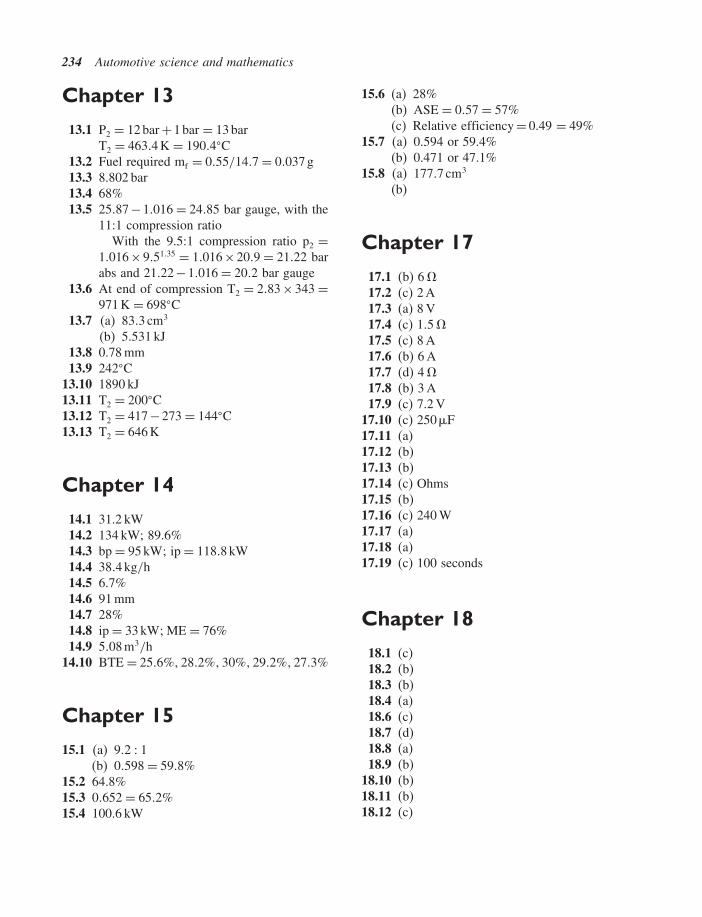
234 Automotive science and mathematics
Chapter 13
13.1 P2 = 12 bar +1 bar = 13 barT2 = 463�4 K = 190�4�C
13.2 Fuel required mf = 0�55/14�7 = 0�037 g13.3 8.802 bar13.4 68%13.5 25�87−1�016 = 24�85 bar gauge, with the
11:1 compression ratioWith the 9.5:1 compression ratio p2 =
1�016×9�51�35 = 1�016×20�9 = 21�22 barabs and 21�22−1�016 = 20�2 bar gauge
13.6 At end of compression T2 = 2�83 × 343 =971 K = 698�C
13.7 (a) 83�3 cm3
(b) 5.531 kJ13.8 0.78 mm13.9 242�C
13.10 1890 kJ13.11 T2 = 200�C13.12 T2 = 417−273 = 144�C13.13 T2 = 646 K
Chapter 14
14.1 31.2 kW14.2 134 kW; 89.6%14.3 bp = 95 kW; ip = 118�8 kW14.4 38�4 kg/h14.5 6.7%14.6 91 mm14.7 28%14.8 ip = 33 kW ME = 76%14.9 5�08 m3/h
14.10 BTE = 25�6%� 28�2%� 30%� 29�2%� 27�3%
Chapter 15
15.1 (a) 9�2 � 1(b) 0�598 = 59�8%
15.2 64.8%15.3 0�652 = 65�2%15.4 100.6 kW
15.6 (a) 28%(b) ASE = 0�57 = 57%(c) Relative efficiency = 0.49 = 49%
15.7 (a) 0.594 or 59.4%(b) 0.471 or 47.1%
15.8 (a) 177�7 cm3
(b)
Chapter 17
17.1 (b) 6 �17.2 (c) 2 A17.3 (a) 8 V17.4 (c) 1�5 �17.5 (c) 8 A17.6 (b) 6 A17.7 (d) 4 �17.8 (b) 3 A17.9 (c) 7.2 V
17.10 (c) 250 F17.11 (a)17.12 (b)17.13 (b)17.14 (c) Ohms17.15 (b)17.16 (c) 240 W17.17 (a)17.18 (a)17.19 (c) 100 seconds
Chapter 18
18.1 (c)18.2 (b)18.3 (b)18.4 (a)18.6 (c)18.7 (d)18.8 (a)18.9 (b)
18.10 (b)18.11 (b)18.12 (c)

Index
Absolute pressure, 151Absolute temperature, 151Acceleration, 30
Angular, 116Centripetal, 117, 118Gravitational- g, 115Linear, 115, 116
Accuracy, 3, 4Adiabatic
Process, 153Compression, 172Expansion, 153
AirComposition of, 185Air-fuel ratio, 9Resistance, 124
Algebra, 29Alternating current, 207Alternator, 197Amplitude, 140Analogue to digital conversion, 225Angles
Of gradient, 127Of friction, 107
Angular motion – equations of, 116Angular velocity, 116ASCII – codes, 11Atom, 196
BalanceEngines, 135Flywheel, 133Reciprocating mass, 135Rotating mass, 132Wheels, 134
Bar chart, 18
Bar – unit of pressure, 62Barometric pressure, 151Bearings, power lost in friction, 110Belt drive, 101Binary
Code, 10System, 10
BODMAS, 7Brake
Mean effective pressure-bmep, 167Power-bp, 158Thermal efficiency, 168Specific fuel consumption – bsfc, 166
BrakesDisc, 112Drum, 103
Braking efficiency, 106
CamsAcceleration, 144Displacement, lift, 145
Calorific value, 184Capacitance, 210Capacitor, 210Carbon
Dioxide, 34Monoxide, 190
Catalytic convertor, 190Centre of gravity, 51Centrifugal force, 118Centripetal force, 118Charles’ law, 152Circle, arc, 46, sector, 46Circuits, 198Class width, 19Composition of fuel, 184

236 Index
CompressionAdiabatic, 153Isothermal, 151Ratio, 9
Compressive stress and strain, 68Complementary angles, 44Computer controlled systems, 11Connecting rod, Effect on balance, 136Conservation of energy, 92Constant pressure cycle, 175Constant volume cycle, 172Consumption of fuel
Fuel consumption curves, 166Coolant temperature sensor, 223Coordinates, 35Coulomb, 214Couple, 85Coordinates, 35Crankshaft
Balance, 135Damper, 143End float, 13Torque, 83Vibration, 143
CurvesPower, 164Torque, 165Bmep, 167Specific fuel consumption, 166
CycleOf operations, 172Otto, 172Diesel, 175Dual combustion, 176Stirling, 178
CylinderEngine, 29Brake, master, 63Volume of, 9
Darlington pair, 221Data, 16Decimal system, 1Deceleration, 106Deciles, 26Degrees of accuracy, 4
Density, relative, 184Diagram
Force, 60Pressure volume, 154Indicator, 160
DieselCycle, 175Fuel, 184
Differential, 123Diode, 217Directed numbers, 11Disc brakes, 103Distance time graphs, 113Double shear, 69Dual combustion cycle, 176Dynamic balance, 133Dynamometer, 158
EfficiencyAir standard, 173Braking, 106Engine, mechanical, 164Machines, 95Relative, 174Transmission, 124Volumetric, 165
EffortMachine input, 95Tractive, 122
Elastic materials, 64Elastic limit, 65Elasticity
Young’s modulus of, 73Electron, 196Electronic
Control unit, 10Devices, 221Principles, 216
Emissions, exhaust, 188End of life vehicles, 77Energy
Chemical, 92Conservation of, 92Conversion, 93Electrical, 206Kinetic, 92

Index 237
Mechanical, 206Potential, 92
EngineBalancing, 135Cycles, 172Performance, 164Torque, 83
Exhaust, emissions, 185Extension, 64
Factors, 6Factor of safety, 74Factorising, 31Falling bodies – gravitational effect, 93Farad, 210Fluid- pressure of, 62Force
And its effects, 58Diagrams, 59Of acceleration, 115Of friction, 111Braking, retardation, 106Centripetal, 118Centrifugal, 118Gravitational, 58Units of, 115
Four wheel drive, 123Fractions, 6Frequency
Distributions, 25Of alternating supply, 208Of vibration, 142Natural, 142
FrictionAngle of, 107Bearing, 110Clutch, 100Coefficient of, 99Force of, 100In a screw thread, 108On an inclined plane, 108
Frictional torque, 110Fuel
Calorific value, 184Cells, 194
Combustion, 184Consumption, 166Curves, 166
Gamma – adiabatic index, 153Gas
Absolute pressure, 151Absolute temperature, 151Laws, 151Specific heat capacity at constant
pressure, 152Specific heat capacity at constant
volume, 151Gates- logic, 225Gauge pressure, 151Gear
Ratio, 9gearbox ratio, 85
Gearbox efficiencyGenerator, 206Gradient, 36Gradeability, 126Gravity – effect of, 58Grouped data, 19Gyration – radius of, 93
Hardness, 75Harmonic – balancer, 138
Motion, 139Heat – form of energy, 149
Sink, 221Heating of gases, 151Hertz, 208Hole, 217Hooke’s law, 64Hydraulic
Pressure, 63System, 63
Ideal cycle, 153Ideal efficiency, 180Ignition, sperk, 185, compression, 186Integrated circuit, 223Impedance, 212Impulse, 143Indicated power, 160
238 Index
Indicator diagram, 160Indices, 5Induction – electro magnetic, 204Inertia, 115Integer, 1Internal combustion engine, 158Isosceles triangle, 45Isothermal process, 152
Jack- as a machine, 94Joule – unit of energy, 92Journal friction, 110Junction diode, 217
Kelvin – temperature scale, 148Kilogram – unit of mass, 62Kilowatt, 90Kinetic energy, 92
Of rotation, 93King pin inclination – KPI, 42Knock, 185
Lamp, 198Law
Boyle’s, 153Charles’, 152Hooke’s, 64
LED, 219Left hand rule, 207Lenz’s law, 208Limit- elastic, 69Linear equations, 116Load
Apparent transfer, 82Loads – on axles, 82Logic gates, 225Loop – pumping, 160Lowest common multiple, 6
MachinePurpose of, 94Law of, 37
MagnetElectro, 204Permanent, 203
MagneticField, 204Flux, 204
MassBalancing, 132Reciprocating, 135Rotating, 93Unit of, 62
Maximum acceleration, 123Mean – arithmetic, 23Mean effective pressure, 160Mechanical advantage – force ratio, 94Mechanical efficiency, 95Meter, 202Mid-ordinate rule, 91Mixture – air fuel ratio, 9Modulus
of elasticity, 73of rigidity, 44
MomentTurning, 79Of inertia, 74Overturning, 129Righting, 129
MomentsPrinciple of, 79
MotionEquations of, 114Newton’s laws of, 115Relation between angular and linear, 117Simple harmonic, 139
Morse test, 164
Natural frequency of vibration, 143Negative
Numbers, 11Temperature coefficient, 203
Newton’s laws of motion, 115n-p-n transistor, 220N-type semiconductor, 217Nitrogen – oxides of, 189
Ogive, 22Ohm, 200Ohm’s Law, 200

Index 239
Open circuit, 202Operations in arithmetic, 7Otto cycle, 173Out of balance force, 134Overturning effect, 62Overturning moment, 129Overturning speed, 129Oxygen sensor, 223
Parallelogram of forces, 60Pascal, 62Percentages, 8Perfect gas, 151Performance
Curves, 164Vehicle, 124
Periodic time, 140Photo diode, 219Pictograph, 18Pie chart, 18Piston
Acceleration, 136Velocity, 50
p-n junction, 217Population, 22Potential difference, 198Power
Absorbed in friction, 110Brake, 158Curves, 167Indicated, 160Transmitted by belt drive, 102Transmitted by clutch, 101
Powers – and roots, 4Pressure, 29
Absolute, 151Brake mean, 167
Pressure-volume diagram, 154Primary force, 136Principle
Of energy conservation, 92Of moments, 79
ProcessAdiabatic, 153Isothermal, 152
Propelling force – tractive effort, 124
Pumping loop, 160Pythagoras’ theorem, 46
Quantity-Vector, 59Quartiles, 25
Radian, 41Radius
Of gyration, 93Of turn, 129
RatioAir-fuel, 9Compression, 9Gear, 9, 85Gearbox, 9Overall gear, 14Velocity – movement, 95
R-C time constant, 210Relative efficiency, 174Relative frequency, 21Resistance
Air, 124Electrical, 200Gradient, 126To motion – tractive, 124
Resistivity, 197Resistors, 201Retardation, 106Rigidity – modulus of, 73Road wheel balance, 134Rolling resistance, 128Rounding – numbers, 4Rotating mass – balance, 132
Safety factor, 74Sampling, 22Screw thread, 108Secondary forces – engine balance, 136Semiconductor, 197Sensor, 223Series, 201Series circuit, 201Sequence of arithmetical operations –
BODMAS, 7Shear stress, 68Short circuit, 203

240 Index
Sine, 49Single cylinder, 135Silicon, 216Skidding speed, 130Specific
Heat capacity, 150Gravity – relative density, 184
Slope of line, 36Square root, 5Standard form, 5Static balance, 133Statistics, 16Steering, 95Straight line law of, 36Strain, 68, 72Stress, 68Strength, 73Suspension, 142
Tangent, 48, 49Temperature
Absolute, 148Kelvin, 148Standard, 48Coefficient of resistance, 203
TensileStrain, 72Stress, 68, 69
Tension, 69Test
Morse, 164Tensile, 69
ThermalCoefficient of linear expansion, 148Efficiency, 168
Theoretical cycleConstant volume, 172Diesel, 175Dual combustion, 176Gas turbine, 180Otto, 172Stirling, 178
Thermocouple, 198Third differential, 123Thrust
Crankshaft end, 12
TorqueBraking, 105Clutch, 100Crankshaft, 83Driving, 127Engine, 83Input, 85Output, 87Work done by, 90
Torsional vibrationFrequency of, 142Damper, 143Of shaft, 142
TractiveEffort, 122Resistance, 123
TransistorBase, collector, emitter, 220Bipolar, 219Common emitter, 221Current gain, 220Darlington pair, 221n-p-n type, 220switch, 225
Transmission efficiency, 124Transposition – transformation – of formulae, 33Triangle of forces, 60Triangles – types of, 45Trigonometrical ratios, 49Truth table, 225Turning moment, 62Twin cylinder engine, 139Twist – angle of, 74
Uniform velocity, 113
Vacuum servo, 78Variables
Dependent, independent, 34Velocity
Angular, 116Average, 114Equations of, 116Of piston, 50Versus time graphs, 113
Index 241
Velocity ratio – movement ratio, 95Vibrations, 141Volt, 200Voltage drop, 200Volume-swept, 9Volumetric efficiency, 165
Watt, 89wheel balance, 134Wind resistance, 124Work
Area under force-distance graph, 91Diagram, 91
Done against gravity, 89Done during expansion and compression
of gas, 154
Yield point, 70Young’s modulus, 73
ZenerDiode, 218Voltage, 218
ZeroAbsolute temperature, 148Emissions vehicle, 194

This page intentionally left blank