autonomous collision avoidance - cal poly
TRANSCRIPT

i
Thomas Stevens
Elliot Carlson
Ian Painter
June 14, 2013
Project Sponsor: Dr. Charles Birdsong
Project Advisor: Dr. Charles Birdsong
Autonomous Collision Avoidance
Final Design Report
Cal Poly San Luis Obispo

ii
Table of Contents Chapter 1. Introduction ............................................................................................................................................. 2
1.1. Objectives ......................................................................................................................................................... 3
1.2. Specifications ................................................................................................................................................... 4
1.2.1. Specifications updates ............................................................................................................................ 7
Chapter 2. Background .............................................................................................................................................. 9
2.1. ESV Student Design Competition ............................................................................................................... 9
2.2. Sensors .............................................................................................................................................................. 9
2.2.1. Radio Detection and Ranging (Radar): ................................................................................................ 9
2.2.2. Light detection and Ranging (LiDAR) ............................................................................................. 10
2.2.3. Ultrasonic .............................................................................................................................................. 10
2.2.4. Image processing ................................................................................................................................. 11
2.2.5. Magnetic ................................................................................................................................................ 12
2.2.6. Infrared Imaging .................................................................................................................................. 12
2.3. Existing Systems ........................................................................................................................................... 14
2.3.1. Mercedes-Benz Brake Assist PLUS and PRE-SAFE®.................................................................. 14
2.3.2. Google Autonomous car .................................................................................................................... 15
2.3.3. MIT Autonomous RC plane .............................................................................................................. 15
2.4. Path Planning Algorithm ............................................................................................................................ 16
2.4.1. Rapidly Exploring Random Tree Algorithm ................................................................................... 16
2.4.2. Model Predictive Controller ............................................................................................................... 16
Chapter 3. Design Development .......................................................................................................................... 18
3.1. Design Flowchart ......................................................................................................................................... 18
3.2. Sensor Technologies Testing ...................................................................................................................... 19
3.2.1. Ultrasonic .............................................................................................................................................. 19
3.2.2. LiDAR/Infrared .................................................................................................................................. 22
3.2.3. Radar ...................................................................................................................................................... 29
3.2.4. Image Processing ................................................................................................................................. 30
3.2.5. Final Decision Matrix .......................................................................................................................... 35
3.3. Conceptual Design Conclusion .................................................................................................................. 35
Chapter 4. Final Design .......................................................................................................................................... 37

iii
4.1. Hardware Development .............................................................................................................................. 38
4.1.1. Final Sensor Selection ......................................................................................................................... 38
4.1.2. LiDAR Mounting Bracket Design .................................................................................................... 38
4.1.3. Powering the LiDAR .......................................................................................................................... 43
4.1.4. Data Acquisition from LiDAR .......................................................................................................... 44
4.1.5. IMU and Wheel Encoders .................................................................................................................. 44
4.1.6. Power Supply ........................................................................................................................................ 44
4.1.7. Key Switch Box .................................................................................................................................... 45
4.1.8. User control .......................................................................................................................................... 47
4.1.9. Video Feedback.................................................................................................................................... 48
4.2. Software Development................................................................................................................................ 49
4.2.1. LiDAR Data collection ....................................................................................................................... 49
4.2.2. Segmentation ........................................................................................................................................ 50
4.2.3. Road Detection .................................................................................................................................... 52
4.2.4. Threat Determination & User to Autonomous Toggle ................................................................. 55
4.2.5. Simulation of Data Parsing and Road detection ............................................................................. 56
4.2.6. Rapidly Exploring Random Tree (RRT) .......................................................................................... 58
4.2.7. MPC ....................................................................................................................................................... 62
4.3. Cost Analysis................................................................................................................................................. 63
4.3.1. System Costs ......................................................................................................................................... 63
4.3.2. Cost Benefit Analysis .......................................................................................................................... 63
Chapter 5. Design Verification .............................................................................................................................. 69
5.1. Testing Procedures ...................................................................................................................................... 69
5.1.1. Testing Results ..................................................................................................................................... 71
5.1.2. Driver Satisfaction Survey .................................................................................................................. 75
Chapter 6. Conclusions and Future Work ........................................................................................................... 77
6.1. Conclusion .................................................................................................................................................... 77
6.2. Future Work/Recommendations .............................................................................................................. 77

iv
Table of Contents Figure 1 Radar System Detecting an Airplane ............................................................................................................. 9
Figure 2 Terrain Mapping using a 3-D LiDAR Sensor ........................................................................................... 10
Figure 3 Ultrasonic Sensor .......................................................................................................................................... 11
Figure 4 Path Planning using Image Processing ...................................................................................................... 11
Figure 5 Stereo Cameras taking Two Pictures Simultaneously .............................................................................. 12
Figure 6 Hall-effect Magnetic Sensor ........................................................................................................................ 12
Figure 7 Traditional Camera Imaging on the Left Compared to Infrared Imaging on the Right .................... 13
Figure 8 Mercedes Braking System ............................................................................................................................ 14
Figure 9 Image obtained by Google Car’s Multiple Sensors .................................................................................. 15
Figure 10 MIT's Autonomous Plane Following RRT generated Path .................................................................. 16
Figure 11 Random Trees Generated by RRT ........................................................................................................... 16
Figure 12 Graphic illustration of the MPC control theory ..................................................................................... 17
Figure 13 Sensor Selection Flowchart ....................................................................................................................... 18
Figure 14 Prototype with Sensor Mounted on Front Bumper (left) and Sensor Stand (right) ......................... 19
Figure 15 Ultrasonic Mounted on Upper Location of Elevated Stand Outside ................................................. 20
Figure 16 Ultrasonic Mounted at a Lower Position on the Elevated Stand Outside ......................................... 21
Figure 17 Ultrasonic Sensor and Sensing Area ........................................................................................................ 21
Figure 18 Sharp IR sensor analog output as a function of distance ...................................................................... 23
Figure 19 IR Sensor Approach and Recede at 20 Hz ............................................................................................. 24
Figure 20 Scanning LiDAR Sensor Experimental Setup ........................................................................................ 25
Figure 21 Rotating IR Sensor (6RPM) @ 20 Hz for 2 Revolutions ..................................................................... 25
Figure 22 Polar Plots for Rotating IR Sensor (Rotation 1 on left, Rotation 2 on right) .................................... 26
Figure 23 Color/Reflectivity experimental setup ..................................................................................................... 26
Figure 24 Effect of color on Infrared signal ............................................................................................................. 27
Figure 25 LiDAR Sensor and 2-D map generated by Scanning LiDAR .............................................................. 29
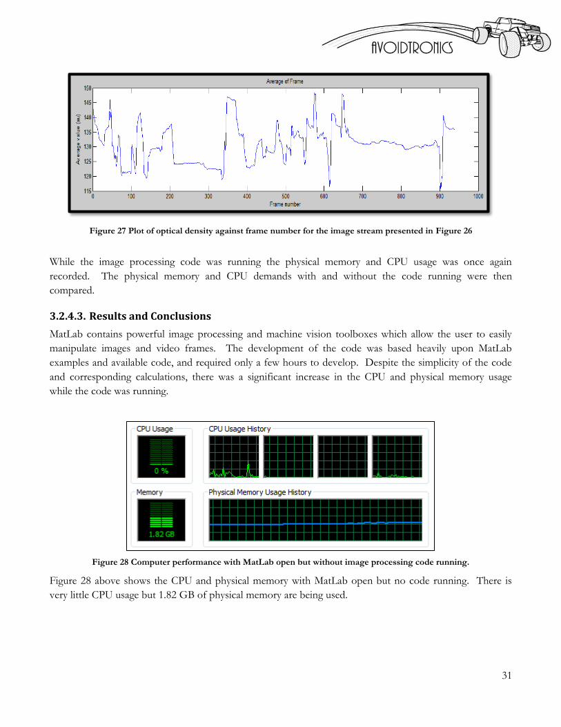
Figure 26 Snapshot of MatLab image processing output ....................................................................................... 30
Figure 27 Plot of optical density against frame number for the image stream presented in Figure 26 ........... 31
Figure 28 Computer performance with MatLab open but without image processing code running............... 31
Figure 29 Computer performance with MatLab open and running image processing code. ............................ 32
Figure 30 Blackfin SRV-1 camera module ................................................................................................................ 34
Figure 31. System overview showing the process flow of the system. ................................................................. 37
Figure 32. Hokuyo UBG-04LX-F01 .......................................................................................................................... 38
Figure 33. Solid model including updated roll cage and LiDAR mounting bracket ........................................... 39
Figure 34. Exploded view of LiDAR Mounting bracket ........................................................................................ 40
Figure 35 Chassis Acceleration in frontal collision test setup ................................................................................ 41
Figure 36 Chassis acceleration as a function of time for the frontal collision setup shown in Figure 34 ....... 42
Figure 37. Circuit diagram for LiDAR Power circuit .............................................................................................. 43
Figure 38. Power supply board with component description ................................................................................ 45
Figure 39. Key box with component labels .............................................................................................................. 46
Figure 40. Inner wiring of Key box with component descriptions ....................................................................... 47

v
Figure 41. Logitec steering wheel and pedal controls ............................................................................................. 48
Figure 42. System Simulink high level block diagram ............................................................................................. 49
Figure 43. egmented Point-Cloud Results and the Actual Test Layout................................................................ 51
Figure 44. Road detection. Note detected obstacles within the roadway and the inwards from of road lines
from the line of cones within the point-cloud. ........................................................................................................ 54
Figure 45. Segmentation simulation screen shots .................................................................................................... 57
Figure 46. LiDAR and Global Coordinate System .................................................................................................. 58
Figure 47 ROAD and ROADLINES variables ....................................................................................................... 60
Figure 48 Geometry of RAND_NODE ................................................................................................................... 61
Figure 49 CHECK_COLLISION visual .................................................................................................................. 62
Figure 50. Lidar scan with filtered data. Obstacles and road bounds are parsed from the data ....................... 72
Figure 51. Experimental setup for reliability test and driver satisfaction survey ................................................. 73
Figure 52. Question from driver satisfaction survey with results .......................................................................... 75
Figure 53. Question from driver satisfaction survey with results .......................................................................... 76
Figure 54. Question from driver satisfaction survey with results .......................................................................... 76
Figure 55 Required Viewing Angle for Full View of Wheel-Base 12 inches from Front Bumper ................... 81
Figure 56 Sensor Size and Available Space Comparison ........................................................................................ 81

vi
Table of Tables Table 1 Engineering Specifications ............................................................................................................................... 4
Table 2 LiDAR Decision MatrixNumber ................................................................................................................. 28
Table 3 Image processing sensor decision matrix.................................................................................................... 33
Table 4 Final Decision Matrix with Sensor Pairing ................................................................................................. 35
Table 5. Coordinate Comparison ............................................................................................................................... 59
Table 6. Bill Of Materials ............................................................................................................................................. 63
Table 7. Crashes by first Harmful Event, Manner of Collision and Crash Severity ........................................... 65
Table 8 Preventable Crashes by first Harmful Event, Manner of Collision and Crash Severity ...................... 66
Table 9. Vehicles involved in Crashes by vehicle type and crash severity ............................................................ 66
Table 10 Preventable Crashes by first Harmful Event, Manner of Collision and Crash Severity For
Passenger cars and Light Trucks ................................................................................................................................ 67
Table 11 Financial loss due to travel delay and property damage by MAIS injury level .................................... 67
Table 12. Calculation of Fatla Equivalents NHTSA Values .................................................................................. 68
Table 13 Total Savings of fleet wide system integration ......................................................................................... 68
Table 14. Final Subsystem testing results .................................................................................................................. 71
Table 15. Results from repeatability testing as well as the two obstacle test ....................................................... 74

vii
ABSTRACT
A steering controlled, autonomous collision avoidance system has been developed by California Polytechnic
State University. This system represents a step in the direction of fully autonomous driving, while allowing
the driver to maintain control of the vehicle during normal driving conditions. In the case of an imminent
collision, the system removes control of the vehicle from the user and autonomously steers around the
obstacles. The final system is able to avoid two static obstacles with a 95% pass rate and one moving
obstacle with a 50% pass rate. With full scale, fleet wide, implementation of this system it is expected that
each year up to 7,222 lives could be saved and over 60,000 injuries prevented. This decrease in the number
of injuries and fatalities would produce a net yearly savings of up to $132 Billion per year.

1

2
Chapter 1. Introduction
The purpose of this project is to create a scaled model of an autonomous car crash avoidance system. The
project is a continuation of two projects, the 2010 “Autonomous Crash Avoidance System” senior project
and the 2012 “A Model Predictive Control Approach to Roll Stability of a Scaled Crash Avoidance Vehicle”
master’s thesis. The system developed by these teams utilizes a 1/10th scale, two-wheel drive remote
controlled car. It uses a Rapidly Exploring Random Tree (RRT) path planning algorithm to determine the
steering inputs required to maneuver the vehicle away from a collision. Stability is addressed with a non-
linear, eight degree of freedom vehicle model-predictive-stability controller.
The scope of the current project is to implement a sensor that will dynamically detect obstacles as well as
the boundaries of the road and feed this data into the control system so that it can react to imminent frontal
collisions. This includes an in-depth study of existing sensor technologies, development of data processing
algorithms, and integration with the existing system. The vehicle will be controlled by a human driver, using
realistic driving controls, until emergency avoidance is required, at which point, the avoidance software will
be automatically activated. The transition from driver to computer control will be implemented similarly to
modern dynamic stability control, such that for small maneuvers the driver should not be aware of any
intervention.
This type of technology has the potential to significantly reduce injury and fatalities from auto accidents.
The National Highway Traffic Safety Administration reports that in the United States in 2010 there were
1,542,000 automotive crashes, which resulted in injury, and 30,196 that resulted in fatalities. Nearly 70% of
all fatal accidents in 2010 involved frontal collisions and over 10% of all fatal crashes involved distracted
drivers. With a computer, which can react hundreds of times faster than the driver and is never distracted,
constantly monitoring ahead of the vehicle to avoid to imminent collisions, over 7000 lives could be saved
each year and significantly more injuries mitigated.
The project was undertaken with the intention of competing at the 5th annual Enhanced Safety of Vehicles
(ESV) student design competition in Seoul, South Korea. Due to the nature of the competition, much of the
to design involve development of an interactive and informative presentation to demonstrate the
technology.

3
1.1. Objectives
This project aimed to select and implement sensors for the purpose of object detection and avoidance on an
existing 1/10th scale RC car. The sensor data is collected and passed into a computer running an RRT
algorithm in real time. The data processing code will be modularly developed such that it could easily be
ported to another system requiring similar inputs. Tangential to the development and implementation of the
sensor system a presentation demonstrating the capabilities of the system was developed for the ESV
Student Design Competition. The interactive presentation offers the audience firsthand experience with
what this technology may feel like when scaled to a full size vehicle. The formal engineering specifications
listed in Table 1 reflect the customer requirements as well as those of the ESV Design Competition. These
requirements were obtained by completion of the Quality Functional Deployment (QFD) found in
Appendix A. The QFD was used to generate, compare, and evaluate formal engineering specifications and
their corresponding metrics. The QFD helped to develop, refine, and evaluate different specifications by
comparing how each specification related to customers concerns. Multiple specifications were determined
by the existing system or project constraints. The operating frequency of the sensor was determined by the
existing 20 Hz system frequency which is limited by the MPC controller. When possible, such as with the
viewing angle, specific target quantities were calculated. The viewing angle was determined from geometric
relations after selecting target horizontal ranges, see 6.2.Appendix B for calculations. A specification table
can be found below and is followed by a justification for each parameter and its assigned value.
4
1.2. Specifications
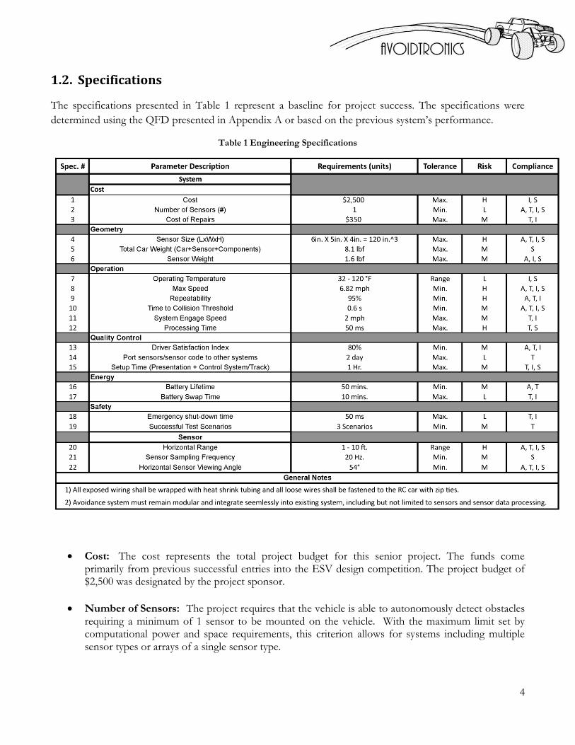
The specifications presented in Table 1 represent a baseline for project success. The specifications were
determined using the QFD presented in Appendix A or based on the previous system’s performance.
Table 1 Engineering Specifications
Cost: The cost represents the total project budget for this senior project. The funds come primarily from previous successful entries into the ESV design competition. The project budget of $2,500 was designated by the project sponsor.
Number of Sensors: The project requires that the vehicle is able to autonomously detect obstacles requiring a minimum of 1 sensor to be mounted on the vehicle. With the maximum limit set by computational power and space requirements, this criterion allows for systems including multiple sensor types or arrays of a single sensor type.

5
Cost of repairs: This specification allows for the measurement of system durability. Cost of Repairs includes the replacement of damaged boards or RC car components. This does not cover the replacement of the primary sensors. Steps shall be taken to mitigate this cost such as providing a protective enclosure for the boards and implementing an emergency system shutdown. Based on the repairs in previous phases of this project a $350 maximum was selected for a tolerable cost of repairs.
Sensor Size/Dimensions: The size was selected to ensure that the sensor would be able to fit into the space currently available on the RC car. The aesthetics of the system were also considered as this project will ultimately be judged on the overall system. A size of 6” x 5” x 4” was determined to be the maximum acceptable size.
Total Car Weight: This specifies the total allowable vehicle weight. This specification includes the existing system, the sensor(s), and all additional hardware. The weight of the system affects the vehicle handling; a car that is too heavy may not be able to execute the maneuvers demanded by the code. If the additional weight is added over the front or rear axle, rather than at the cg of the vehicle, it is possible to bottom out the suspension with less weight than if added at the cg. To obtain the maximum vehicle weight the weight needed to bottom out the suspension, when placed over the front axle, was added to the existing vehicle weight. A weight of 8.1 pounds was selected as a maximum value that cannot be exceeded.
Sensor Weight: Since the sensor is located directly above the front axle, the location most likely to cause the suspension to bottom out,, a limit was place on its weight. This value was determined by placing known weights over the front axle and observing when the front suspension bottomed out. This value was selected as the maximum value that could be tolerated to maintain existing RC car performance. It should also be noted that stiffer springs can be purchased for the RC car, thus allowing a larger sensor weight.
Operating Temperature: The sensor and system must be able to tolerate operation in varied conditions to allow for international as well as domestic use and shipping conditions.
Max Speed: The max speed at which the system can reliably execute collision avoidance maneuvers was determined by previous projects to be 1/10th the speed of a full size vehicle traveling at freeway speeds. This resulted in a maximum avoidance maneuver speed of 6.83 mph. This speed is limited by the top speed of the vehicle and the processing power of available.
Repeatability: Successfully repeating collision avoidance is one of the main goals of this project. A value of 95% was selected as a target value instead of 99.9% due to limited project resources. This represents the target reliability for the 3 avoidance scenarios specified in “Successful Test Scenarios”
Time to Collision Threshold: The system shall not react to detected objects unless the vehicle is determined to be within 0.6 seconds of a collision. This benchmark value came directly from the Mercedes Benz PreSafe Automatic Braking System, which engages full sbraking 0.6 seconds from a collision. This value takes into account the fact that not all detected objects pose an
6
immediate risk of collision. A common example is an obstacle traveling towards the vehicle but in the other lane.
System Engage Speed: The system will not engage at speeds below 2 mph. This speed was chosen to prevent the system from engaging at residential driving speeds or below. At these speeds a collision is extremely unlikely to be fatal and an autonomous maneuver could cause more harm than the collision.
Processing Time: The total processing time for one iteration of the system must be less than 50 milliseconds. The total processing time includes data transmission, data parsing, and RRT & MPC processing. The selected value, 50 milliseconds, is the predetermined simulation frequency of the MPC algorithm. Failure to meet this specification may leave the system blind to obstacles or without crucial steering commands for multiple iterations.
Driver Satisfaction Index: The driver satisfaction index was created to obtain feedback from drivers using the system and their reaction to the technology taking control of the vehicle, temporarily, to avoid obstacles. This value will attempt to quantify the driver experience of the transitions from user to computer control and vice-versa. A value of 80% was chosen as the target because many people have a negative reaction to the idea as well as different driving styles, which the computer may interfere with (most-likely for the good of the driver). Our system will do its best to please the drivers, but not every driver can be satisfied simultaneously. The index quantity for the system will be obtained thru survey and first-hand experience of operating the crash avoidance system, specifically relating to handling, reaction to losing control during collision avoidance, and the regain of control.
Sensor System Porting: The code developed for this system must be able to be ported into another system within 2 days. This assumes that the dynamic modeling for the MPC controller has been previously completed and that the system inputs are the same as the inputs found in this system. This specification allows for the code to be easily implemented on another vehicle as this project progresses.
Setup Time (Presentation and Track): The presentation material and driving track must be able to be set up in less than one hour. The setup time includes, but is not limited to, the driver controls, the video feedback system, the track itself, the computer control system, and the presentation material. This specification is required by the time constraints of the ESV international competition.
Battery Lifetime: The batteries, Li-ion and car battery must last a minimum of 50 minutes. This specification represents the target lifetime to power sensors, control boards, communication modules, and the vehicle itself. This specification was determined to allow near continuous presentation of the system at the ESV international competition and during the driver perception survey.
Battery Swap Time: The batteries, Li-ion and car battery, must be able to be swapped in less than 10 minutes. It is essential that system maintenance time be minimized during presentations in order to maintain the audience’s attention.

7
Emergency System Shut Down Time: In an emergency situation the system must be able to be shut down in less than 50 milliseconds. Due to the potential for damage to the system and possible harm to bystanders in the event of a system failure an emergency shutdown is to be implemented. This will allow the operator to shut the system down from the driving controls. The value was selected to assure that the system shuts down prior to executing the subsequent steer command.
Successful Test Scenarios: Three Three different test scenarios involved most often in frontal collisions will be targeted for collision mitigation. These scenarios all involve the target vehicle traveling down a straight roadway having to avoid obstacles in three different scenarios. The scenarios are as follows: a stationary object in the middle of the roadway, a obstacle traveling across the target vehicles path, an obstacle in the vehicle path that moves as the vehicle gets within close proximity.
Horizontal Range: The system must be able to detect obstacles that are more than 1 foot away and less than 10 feet away from the vehicle. The maximum value was selected using the time to collision threshold and the maximum speed previously determined. The value was also compared against similar threshold values set by the Mercedes Benz PreSafe Automatic Braking system and were found to be similar. Due to the limitations of the hardware the vehicle cannot avoid a similarly sized obstacle within 22 inches of the front of the vehicle so a minimum range of 1 foot is acceptable.
Sensor Sampling Frequency: The sensor must be able to sample data at a frequency of at least 20 Hz. This value was selected to assure that there is a new scan for each iteration of the system. At lower frequencies it is possible that two subsequent paths could be planned using the same data which may not accurately represent the environment.
Horizontal Sensor Viewing Angle: The horizontal viewing angle of the sensor must be at least 54 degrees. The horizontal viewing angle is a measure of the minimum angle that the sensor can detect in a 2D plane parallel to the ground. This angle was determined from the minimum horizontal range and the width of the wheelbase of the vehicle. See 6.2.Appendix B for a complete calculation.
1.2.1. Specifications updates
Throughout the design process additional specifications were determined that would allow the team to
internally measure the success of the design. Additionally some specifications were updated to more
accurately represent the project goals. In cases where the specification was changed, the system will be
tested against both the original and the final metric.
Driver Satisfaction Survey: It was determined that rather than measuring the success of the survey by the 80% acceptance rate originally stated it would be more appropriate to measure success by the number of participants surveyed (minimum of 30). By not seeking to achieve a certain approval rating the results of the survey are expected to be less biased by the team’s goal.

8
Detected Obstacle State: The frontal area and position of the detected obstacle must be within 10% of actual position and frontal area of the obstacle. The Detected Obstacle state seeks to evaluate the accuracy of the data from the LiDAR as well as the accuracy of the data parsing algorithms. It was determined that frontal are was a more acceptable measure than obstacle volume due to the 2D scanning.
Avoid Two Static Obstacles: The test vehicle must be able to avoid two static obstacles 8 out of 10 times. This specification seeks to test the system’s ability to handle situations with multiple obstacles. 80% was selected as the acceptable minimum due to its relative complexity in comparison to the one obstacle test

9
Chapter 2. Background
The following section describes existing sensor technologies as well as their implementation in various
collision avoidance technologies.
2.1. ESV Student Design Competition
The Enhanced Safety of Vehicles (ESV) student design competition is a three tiered, international design
competition. Student design teams submit a project proposal declaring their intent to develop a vehicle
system in one of 15 different categories. The categories include but are not limited to: collision avoidance,
electric vehicle safety, and distraction mitigation. Upon review of the project proposals teams are selected
to compete at a regional level. At the regional level the designs are presented to a panel of judges and are
critiqued on the basis of technological advancements, scalability, and vehicle safety improvements. The top
three teams from the North American, European, and Asian regions are selected to present at the ESV
international conference in Seoul, South Korea in May 2013. The top team at the conference, as judged by
the international panel of judges, is named the winner of the 2013 student design competition.
2.2. Sensors
A brief description of existing sensor technologies is presented below.
2.2.1. Radio Detection and Ranging (Radar):
Radar sensors transmit high frequency radio pulses and record the time required for the signal to reflect off
of an object and return to the receiver. The Doppler frequency shift of the returned signal is also recorded.
The recorded data is used to calculate the position and velocity of the object. Figure 1 depicts a radar system
emitting a series of radio pulses, which are then reflected off of the metallic surface of an airplane and
returned to the sensor. This data would then allow the sensor to determine the position and velocity of the
airplane.
Figure 1 Radar System Detecting an Airplane
There are two main types of radar detectors with applications in vehicle collision avoidance. Pulsed Doppler
(PD) Radar is the most common and operates on the Doppler principle, which states that all objects will
exhibit a frequency shift from the transmitted signal to the received signal. This frequency shift is what

10
allows the radar to detect the velocity of an object. Frequency Modulated Continuous Wave (FMCW) radar
operates similarly to the image processing discussed in section 2.2.4. The FMCW radar breaks the detection
area into small sections and uses background subtraction, the process of overlaying two consecutive frames
and removing what is the same, to detect changes or moving objects.
2.2.2. Light detection and Ranging (LiDAR)
LiDAR operates on the same basic principles as radar. High frequency light waves, often produced by a
laser, are emitted and the time required for the signal to reflect back as well as the Doppler shift are
recorded. The emitted light usually has an extremely short wavelength in the ultraviolet or infrared region.
The high frequency waves of the LiDAR sensor are focused in a smaller beam than a radar sensor. This
results in a detection area that is orders of magnitude smaller, but with a less scattered, stronger reflected
signal. In order to overcome the small beam width of the laser, LiDAR detectors usually involve a rotating
mirror that directs the beam through a horizon and vertical viewing angle allowing the sensor to scan over a
greater area.
Figure 2 Terrain Mapping using a 3-D LiDAR Sensor
Figure 2 above shows a large terrain area which was mapped using a three dimensional LiDAR sensor. The
sensor capturs the contours of the terrain and the resulting map could be used for aircraft navigation or
topographic map generation.
2.2.3. Ultrasonic
Ultrasonic sensors use the same principles as radar and LiDAR, but emit ultrasonic sound waves, which are
reflected off of the object. The reflected waves are received and the time delay is used to determine the
position of the object.
11
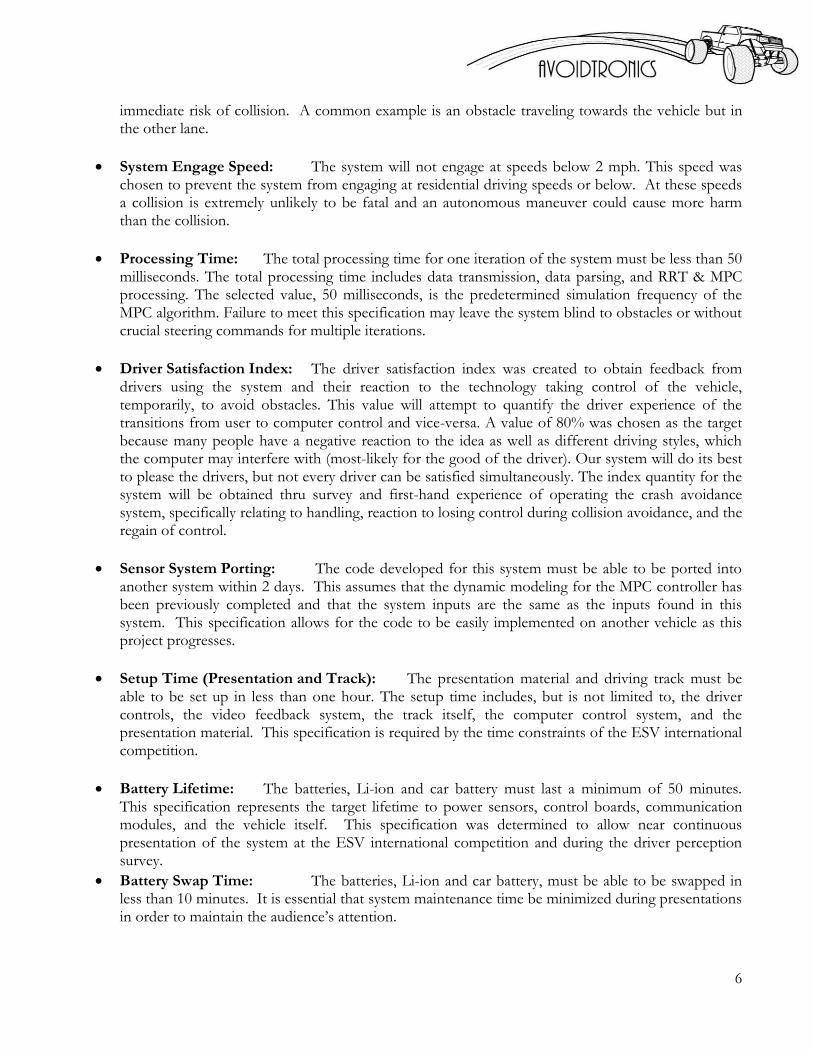
Figure 3 Ultrasonic Sensor
Figure 3 shows a simple ultrasonic sensor. The metallic, cylindrical protrusions are the emitter and receiver
for the sensor, while the printed circuit board provides the electronics to convert the ultrasonic wave into an
electrical signal.
2.2.4. Image processing
Image processing involves taking a video of the surrounding and using pixel data and image processing
software to extract information from the video. The software can be developed to extract various objects
from the video such as moving objects, obstacles, or roads. The angular position of these objects can then
be determined, however, the distance from the camera cannot be accurately determined without further
sensor input.
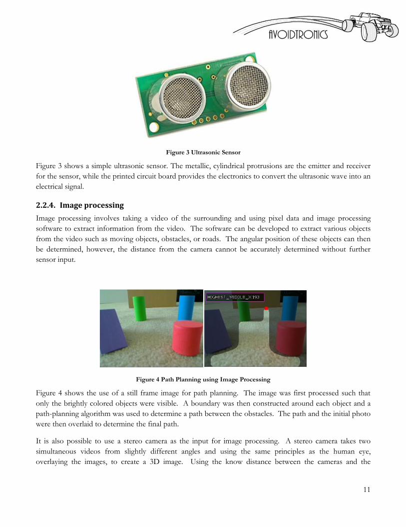
Figure 4 Path Planning using Image Processing
Figure 4 shows the use of a still frame image for path planning. The image was first processed such that
only the brightly colored objects were visible. A boundary was then constructed around each object and a
path-planning algorithm was used to determine a path between the obstacles. The path and the initial photo
were then overlaid to determine the final path.
It is also possible to use a stereo camera as the input for image processing. A stereo camera takes two
simultaneous videos from slightly different angles and using the same principles as the human eye,
overlaying the images, to create a 3D image. Using the know distance between the cameras and the

12
difference in angle between the two images it is possible to detect both distance and angular position of an
object.
Figure 5 Stereo Cameras taking Two Pictures Simultaneously
Figure 5 shows the output of a stereo camera system. The two photos in the Figure 5 are slightly offset
allowing the dog’s paw to be seen in the image on the left, but not in the image on the right. This difference
in the images would be used to determine the position of the dog’s paw and its distance from the cameras.
2.2.5. Magnetic
Magnetic sensors use magnetic fields to detect proximity. The magnetic sensor detects if there is a magnetic
field, and if so returns a binary high/low signal to indicate that there is an object in the magnetic field of the
sensor. There are many types of magnetic sensors; however all require that the object being sensed is
magnetic, meaning that a magnetic sensor would not be able to detect a pedestrian.
Figure 6 Hall-effect Magnetic Sensor
2.2.6. Infrared Imaging
Infrared imaging uses the same principles as a camera, where the intensity and wavelength of light is
captured, however, the light captured is outside of the range of human vision. The wavelength for infrared
can be as long as 14,000 nanometers (450-750 nanometers for visible light). This allows infrared cameras to
be used at night as well as during the day and to capture thermal gradients in the subjects being
photographed.

13
Figure 7 Traditional Camera Imaging on the Left Compared to Infrared Imaging on the Right
Figure 7 shows the difference between an image seen by a traditional camera and by an infrared camera. In
the infrared image the temperature gradient of the person produces different wavelengths of radiation,
producing the image seen. It is also possible to detect the radiation given off by the person’s hands even
though they may not be visible to the human eye.

14
2.3. Existing Systems
The following section presents a brief review of existing collision avoidance systems. The sensors used for
each system are also presented.
2.3.1. Mercedes-Benz Brake Assist PLUS and PRE-SAFE®
High end Mercedes come equipped with Brake Assist PLUS and PRE-SAFE® which implement audio cues
and automatic braking, respectively, if a collision is detected. Brake Assist PLUS makes auditory and visual
cues to the driver if a potential collision is detected. It simultaneously calculates the braking force necessary
to stop the vehicle in time and makes that force available as soon as the driver touches the brake pedal. If
the driver does not respond to the cues, the PRE-SAFE® system initiates 40% braking 1.6 seconds from a
detected impact and full braking .6 seconds from impact. All environment data is collected using one long
range radar detector with a range of 600 ft and 2 short range radar detectors with an 80° viewing angle and
90 ft range.
Figure 8 Mercedes Braking System

15
2.3.2. Google Autonomous car
Google is currently developing a car that is able to autonomously navigate all roads. While the full details of
the autonomous car are beyond the scope of this project, how the car detects and responds to obstacles is
relevant. The Google car uses a combination of a Velodyne 64 beam LiDAR detector, GPS, 4 radar
detectors, and image processing in order to create a 3D map of the environment. This map is then
processed by a computer to determine which objects are permanent, i.e. lamp posts and mailboxes, and
which objects are transient, i.e. pedestrians and cars. This information is then used by the vehicle software
to determine the ideal path to avoid colliding with any of the obstacles.
Figure 9 Image obtained by Google Car’s Multiple Sensors
2.3.3. MIT Autonomous RC plane
MIT has recently developed an RC plane that is capable of autonomous flight over a pre-programmed
route. The plane uses an onboard LiDAR sensor to map the environment and uses the mapped
environment to identify obstacles and react accordingly. The RC plane uses the RRT path-planning
algorithm described in section 2.4.1 to avoid obstacles at speeds up to 25 miles per hour.

16
Figure 10 MIT's Autonomous Plane Following RRT generated Path
2.4. Path Planning Algorithm
2.4.1. Rapidly Exploring Random Tree Algorithm
The Rapidly Exploring Random Tree (RRT) Algorithm is an algorithm used for finding a solution to high
dimension search spaces. In this example a 2D space with arbitrarily placed physical obstacles will be
discussed. In a 2D space the algorithm starts with an initial search node and places a second node that is
then connected to the first with a straight line. A third point is then added and is connected by a straight
line to the nearest point along the previous line. Subsequent points are added and connected to the tree,
causing it to grow. If a node or line intersects a boundary condition, in this case an obstacle, that branch of
the tree is terminated and the tree explores other possible solutions.
Figure 11 Random Trees Generated by RRT
2.4.2. Model Predictive Controller
Model Predictive Control (MPC) is a method of control for complex multivariable systems. The concepts
presented here will be developed using the example of a vehicle executing collision avoidance maneuvers
with velocity and steering control. At each processing step the state of the system is sampled, in this system
reading in steer angle and velocity, and the cost function given by Equation 1 is minimized for a future
timestep [t,t+T].
(1)
With:
= i th controlled variable (e.g. measured position)

17
= i th reference variable (e.g. required position)
= i th manipulated variable (e.g. steer angle)
= weighting coefficient reflecting the relative importance of
= weighting coefficient penalizing relative big changes in
The resulting system inputs are executed – in the example case a small change in steer angle or velocity- and
the state of the system is once again sampled. The calculations are repeated for the now current time step.
Figure 12 Graphic illustration of the MPC control theory

18
Chapter 3. Design Development
The main design decision of the project is the sensor selection. This section outlines the procedure
undergone to select a sensor with each section highlighting a different sensor technology.
3.1. Design Flowchart
The flow chart shown in Figure 13 is the process that was used in choosing a sensor system. The analysis
begins with five feasible sensor types: ultrasonic, infrared, LiDAR, radar, and image processing. The
ultrasonic, infrared, and image processing were subjected to testing. The other sensors, being more
expensive, could not be tested. However these sensor types were either modeled or researched. Then the
systems were compared in a series of decision matrices. The flowchart acts as a guide to our design process,
which is outlined in more detail in the following sections.
Ultrasonic
Infrared
Radar
Lidar
Image Processing
Testing With Model
Testing With Model
Noisy, Inaccurate
Lack of info & products
Small Range
Good 2-D Scanning
Decision Matrix
Decision Matrix
SICK S100
BlackfinCameraModule
FinalDecision Matrix
Camera & Lidar Combo
MATLABTesting
Hokuyo Lidar
Figure 13 Sensor Selection Flowchart
19
3.2. Sensor Technologies Testing
The following section describes the testing conducted for each sensor technology considered. The results
of the testing are also presented. Based upon the test results a series of products were selected for both
image processing and LiDAR sensors and were compared in decision matrices.
3.2.1. Ultrasonic
The following section details the testing conducted with an ultrasonic sensor.
3.2.1.1. Experimental Concept
In order to evaluate ultrasonic sensor's ability to detect an obstacle, a prototype platform was setup on a
small RC car by attaching a microcontroller and reading data from an ultrasonic sensor. The influence of
environmental conditions such as operating the sensor inside and outside was also observed to evaluate how
well this sensor technology will perform in a crowded presentation environment. Mounting locations were
also systematically changed to determine any interferences or any noise that may be exist when placed at
various points on the vehicle.
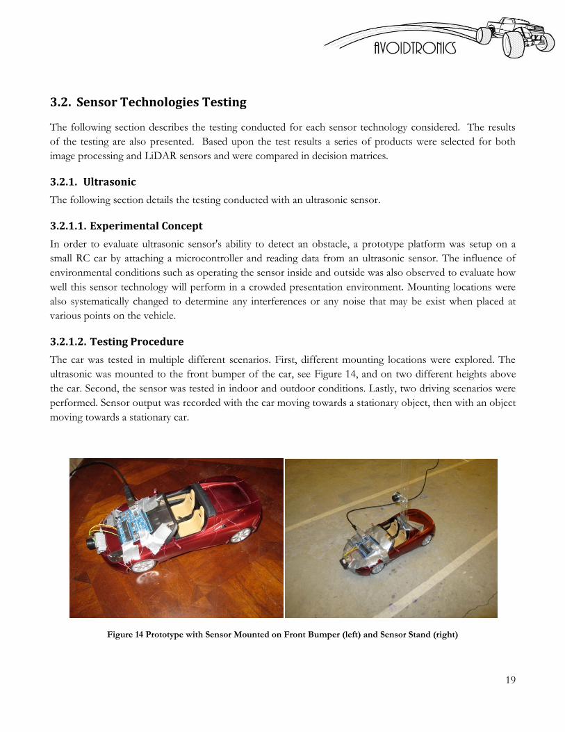
3.2.1.2. Testing Procedure
The car was tested in multiple different scenarios. First, different mounting locations were explored. The
ultrasonic was mounted to the front bumper of the car, see Figure 14, and on two different heights above
the car. Second, the sensor was tested in indoor and outdoor conditions. Lastly, two driving scenarios were
performed. Sensor output was recorded with the car moving towards a stationary object, then with an object
moving towards a stationary car.
Figure 14 Prototype with Sensor Mounted on Front Bumper (left) and Sensor Stand (right)

20
3.2.1.3. Results
The effects of mounting location on the car are very important with the ultrasonic sensor. If
mounted too low, as in the case with the sensor mounted on the front bumper, the sensor will detect the
ground in front of the car. This diminishes the range drastically of the sensor. By mounting the sensor
higher above the car, see Figure 14, much better data is received from the sensor. Another consideration
when using ultrasonic sensors is the effects of indoor versus outdoor use. In an outdoor setting the sensor is
fairly good at picking out at accurately detecting a single object. However in a crowded room the sensor will
detect only the closest object in its range, which may not be the object that is desired to detect. The
ultrasonic consistently output data with excessive noise. This was partially due to vibrations of the sensor.
When the sensor was mounted higher on the mount it vibrated more causing larger spikes in the output.
Due to the noise, output filtering would be required with the system to eliminate false data. From these tests
it became evident that one ultrasonic would not be sufficient in determining the state of the obstacle.
Additionally, the ultrasonic can only detect the obstacle’s distance and not the angle it is at from the car. For
these reasons the ultrasonic is not a good choice for the project.
Figure 15 Ultrasonic Mounted on Upper Location of Elevated Stand Outside
Figure 15 shows the output when the model was driven straight towards a stationary object. The noise
shows that vibrations are a noteworthy issue when considering mounting the sensor(s). This was caused by
sudden accelerations and the wobble of the sensor mount. The red line shows the data after being filtered
with a ten point average.

21
Figure 16 Ultrasonic Mounted at a Lower Position on the Elevated Stand Outside
Figure 16 shows the output of an ultrasonic sensor with a 2ft obstacle moving straight towards it. The
sensor begins detecting the object at about 5s. The object was moved not at a constant velocity from 5 to 13
seconds causing the variation in output. From 14 to 20 the object was moved towards the sensor at a
constant velocity and causing a fairly smooth curve until at 20 seconds the object moved passed the sensor.
This test was conducted outside to ensure no detections other than the obstacle.
3.2.1.4. Product Tested
LV-Max Sonar EZ0
Figure 17 Ultrasonic Sensor and Sensing Area

22
Pros
Cheap ($40)
3-D beam
Small
Analog/Serial Cons
Multiple sensors required for azimuth angle
Noise (filtering required)
Firing Offset may be required
Effected by acceleration
Requires high mounting to not detect ground
Works better outside
3.2.2. LiDAR/Infrared
The following section details the experiments and conclusions relating to the LiDAR and Infrared sensors.
3.2.2.1. Experimental Concepts
In order to evaluate LiDAR and infrared (IR) sensor technology without testing an expensive unit an
experimental setup consisting of an IR sensor was mounted to a slowly rotating platform to emulate a
scanning LiDAR sensor. This test was performed for both qualitative and quantitative information regarding
the effectiveness of scanning range finding technologies. This was considered a valid approach because both
sensor technologies are subject to most of the same pitfalls, such as how the surface color and reflectivity of
the obstacle influence the sensor output. The color dependence of the IR sensor was investigated by reading
values from the sensor at a fixed distance from a cardboard presentation board from spots colored different
colors. The amount of power reflected from the emitted beam is how this particular sensor detects range. In
order to verify this expected power relationship, which we can expect to drop off as distance to some
power. A power curve was fit to data taken from the sensor at various distances from an obstacle. This
particular IR outputs an analog value representing the power of the reflected beam. Numerous values were
taken at fixed distances from the sensor in 1in. increments. This data was then fit to a power curve to
observe and verify the power and range relationship.
3.2.2.2. IR Approach and Recede Test Procedure
In this test a Sharp IR sensor was mounted to the front bumper of the test vehicle shown in Figure 14. The
vehicle was driven towards an object until the front bumper made contact with the object and then backed
away from the object until the sensor could no longer detect the object.

23
3.2.2.3. IR Approach and Recede Results
A power curve was fit to the relation between distance and sensor output to verify the power law nature of
intensity to drop off as a function of distance to some power (the inverse square law). The results agreed
very well with a power relationship and the non-linear distance relationship was verified successfully, as can
be seen in Figure 18.
Figure 18 Sharp IR sensor analog output as a function of distance
Figure 19 shows the output for an IR sensor as a vehicle approaches, reaches a close range, and then
recedes. It is apparent that there is a discontinuity between the approach and the recession of the obstacle.
This occurs for IR sensors when an obstacle is too close, which gives bad data. This discontinuity could
potentially be eliminated through the use of filtering and comparing the output to what is physically
possible. A ten-point average is also shown in red, which shows rather good agreement between the raw and
filtered data with only a same amount of noise. Another note to make is the non-linear region that exists in
the middle of the output region of the sensor.

24
Figure 19 IR Sensor Approach and Recede at 20 Hz
3.2.2.4. Scanning LiDAR Emulation Test Procedure
The setup for this experiment, seen in Figure 20, consisted of an IR sensor affixed to a slowly rotating
microwave turntable motor raised on a stationary piece of 2x4. This experiment aims at simulating a
scanning laser rangefinder to evaluate how effectively a prepackaged product may perform and what value
the concept of scanning laser rangefinder holds for completing the functional requirements of the project.
In particular, reliability was investigated by comparing data obtained from stationary objects within the
sensors range for multiple revolutions in order to see how repeatable the sensor output was. A polar map
was drawn with the data obtained to see how effectively an environmental map can be drawn, while
observing how much data processing, if any, will be required to obtain an accurate map that will be passed
to the avoidance algorithm.

25
Figure 20 Scanning LiDAR Sensor Experimental Setup
3.2.2.5. Scanning LiDAR Emulation Results
The sensor output for a slowly rotating IR sensor as a function of time for multiple revolutions can be seen
in . The sensor was rotated for two continuous rotations for comparison, hence the repeating pattern in the
graph. Each bump represents a physical object seen by the sensor during its rotation. Figure 22 shows the
polar plot of the experiment.
Figure 21 Rotating IR Sensor (6RPM) @ 20 Hz for 2 Revolutions
Error! Reference source not found. shows the consistency of the technology and its ability to affectively
draw and environmental map with high accuracy and repeatability without the use of filtering. The sensor
also was able to distinguish 3 legs of a chair less than ½” in diameter for both revolutions, which can be
seen in the polar plot as the three sharp spikes closely together.

26
Figure 22 Polar Plots for Rotating IR Sensor (Rotation 1 on left, Rotation 2 on right)
3.2.2.6. Color/Reflectivity Test Procedure
The setup for this experiment, as seen in Figure 23, consisted of placing a Sharp IR sensor a fixed distance
of 10 inches from a matte cardboard presentation board. Sensor data was pulled from the sensor using a
microcontroller for a period of time. All the data was then average to obtain an average output value for
each color.
Figure 23 Color/Reflectivity experimental setup

27
3.2.2.7. Results Color/Reflectivity
The effect of different colored obstacles on the sensor output can be seen to have a slight difference
between colors, especially between black and white colored surfaces. However, this value only deviated by
2% for all tested colors as can be seen in Figure 24, so for the scope of this project reflectivity is not going
to be considered a substantial factor affecting performance.
Figure 24 Effect of color on Infrared signal
3.2.2.8. Product Selection
In , five LiDAR sensors that are within the budget are compared in a decision matrix. Each sensor is
compared based on six criteria: Cost, Size, Power Source, Range, Viewing Angle, and Scan Frequency. Each
of these six criteria is assigned a weight. Scan frequency is the highest with a 30% weight and viewing angle
is the lowest at 5%. The weights of each criterion add up to 100%. Each sensor is given an unweighted
score between one and zero, one being the highest, zero the lowest. The unweighted score is chosen based
on how well that system performs in that category compared to the other sensors. So the best sensor in that
category will receive score of 1. The unweighted score is then multiplied by the criteria weight to get the
weighted score, seen in the W column. The weighted scores for each sensor are summed and shown in the
Total row. A perfect sensor would receive a 100 in this box. The LiDAR with the highest score is the SICK
S100 Scanning LiDAR with a score of 67. This sensor has the best scanning frequency at 40Hz. All the
other sensors only have a scan frequency of 10Hz. However the SICK S100, does not meet the weight or
size specification, at 4” x 4”x 6” and 2.6 lbs. The SICK S100 is also fairly expensive at $2000. The next
highest scoring LiDAR is the URG-04LX-UG01, this sensor is substantially cheaper at $1174, but it doesn’t
meet the scanning frequency spec of 20Hz. With a 10 Hz scan time the sensor will not be able to scan as

28
fast as the Matlab code runs. So the car will get new sensor data once every two cycles of commands to the
car. Meaning the car will be making “blind” decisions every other cycle. The third highest scoring lidar the
UBG-04LX-F01 meets all the specifications but the cost. At $2850 dollars the lidar is above the budget by
$350. Since all the sensors do not meet our specifications, none can be chosen for our final system unless
the specifications are revised.
Table 2 LiDAR Decision MatrixNumber
Criteria
Weight (%)
Sensor
UR
G-0
4LX
(H
ok
uyo
)
UB
G-0
4LX
-F0
1
(H
oku
yo
)
UR
G-0
4LX
-UG
01
(H
oku
yo
)
UB
G-0
5LN
(H
oku
yo
)
S1
00
(S
IC
K)
U W U W U W U W U W
1 Cost 25 0.3 7.5 0 0 0.9 22.5 0.7 17.5 0.4 10
2 Size 15 1 15 0.7 10.5 1 15 0.7 10.5 0.2 3
3 Power Source 10 1 10 0.5 5 1 10 0.5 5 0.6 6
4 Range 15 0.5 7.5 1 15 0.5 7.5 0.7 10.5 1 15
5 Viewing Angle 5 1 5 1 5 1 5 0.7 3.5 0.7 3.5
6 Scan
Frequency 30 0.2 6 1 30 0.2 6 0.2 6 1 30
Total 100 51 65 66 53 67
Spec. Justification
1) The Lidar models were chosen based on feasibility of use and price range
2) Specifications not seen in the Criteria were either not comparably different between sensors or not as relevant as chosen criteria

29
3.2.2.9. Product Analysis
The Hokuyo URG-04LX-UG01 Scanning Laser Rangefinder as seen in Figure 25, is presented in the
following section.
Figure 25 LiDAR Sensor and 2-D map generated by Scanning LiDAR
Pros:
Range (12ft)
Viewing Angle (240 degrees)
Accurate
Size
Repeatability Cons:
2-D
Expensive ($1174)
Scan time (100ms)
Non-linear output regions
3.2.3. Radar
Radar sensors seemed to be a promising technology. They are capable of long distance sensing and are
commonly used on full scale cars. For example, radar is used in the Mercedes Pre-Safe system. However,
after thoroughly researching for radar sensors, none were found that meet the project specifications mainly
due to budgetary constraints. Also, the radar sensors the previous teams had used did not have any
specification documentation with them and no data sheets could be found on the internet. Due to lack of
information on the technology and lack of available products, radar sensors are not a feasible sensor system
for the project.

30
3.2.4. Image Processing
The following section presents analysis of basic image processing as well as a comparison of selected camera
modules against project specific metrics.
3.2.4.1. Experimental Concepts
Image processing is a powerful tool that allows the user to extract detailed information from real-time
videos. The primary drawbacks of image processing are the high computing overhead required and the
complexity of the code. In order to test the computing power needed to run a simple image processing
routine a basic image processing code was developed using MatLab.
3.2.4.2. Experimental Procedure
First, code was developed allowing the user to operate the webcam for a windows based platform. The user
is able to select the desired frame rate, determining the amount of processing that will be needed. Figure 26
below shows a snapshot of the video output displayed to the user.
Figure 26 Snapshot of MatLab image processing output
Before beginning the MatLab program a baseline for the physical memory and CPU usage of the computer
was recorded. The code was then initialized. As each frame was being displayed the frame was converted to
a grayscale image in the background and the average optical density of the frame was calculated. The optical
density versus time was then graphed alongside the image. Figure 27 below shows a graph of the average
optical density versus frame number.
31
Figure 27 Plot of optical density against frame number for the image stream presented in Figure 26
While the image processing code was running the physical memory and CPU usage was once again
recorded. The physical memory and CPU demands with and without the code running were then
compared.
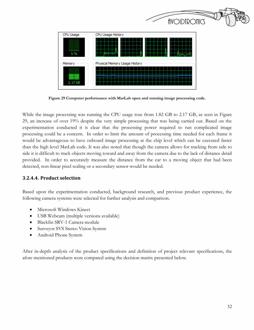
3.2.4.3. Results and Conclusions
MatLab contains powerful image processing and machine vision toolboxes which allow the user to easily
manipulate images and video frames. The development of the code was based heavily upon MatLab
examples and available code, and required only a few hours to develop. Despite the simplicity of the code
and corresponding calculations, there was a significant increase in the CPU and physical memory usage
while the code was running.
Figure 28 Computer performance with MatLab open but without image processing code running.
Figure 28 above shows the CPU and physical memory with MatLab open but no code running. There is
very little CPU usage but 1.82 GB of physical memory are being used.
32
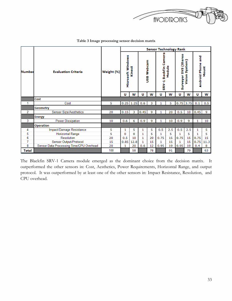
Figure 29 Computer performance with MatLab open and running image processing code.
While the image processing was running the CPU usage rose from 1.82 GB to 2.17 GB, as seen in Figure
29, an increase of over 19% despite the very simple processing that was being carried out. Based on the
experimentation conducted it is clear that the processing power required to run complicated image
processing could be a concern. In order to limit the amount of processing time needed for each frame it
would be advantageous to have onboard image processing at the chip level which can be executed faster
than the high level MatLab code. It was also noted that though the camera allows for tracking from side to
side it is difficult to track objects moving toward and away from the camera due to the lack of distance detail
provided. In order to accurately measure the distance from the car to a moving object that had been
detected, non-linear pixel scaling or a secondary sensor would be needed.
3.2.4.4. Product selection
Based upon the experimentation conducted, background research, and previous product experience, the
following camera systems were selected for further analysis and comparison.
Microsoft Windows Kinect
USB Webcam (multiple versions available)
Blackfin SRV-1 Camera module
Surveyor SVS Stereo Vision System
Android Phone System
After in-depth analysis of the product specifications and definition of project relevant specifications, the
afore mentioned products were compared using the decision matrix presented below.
33
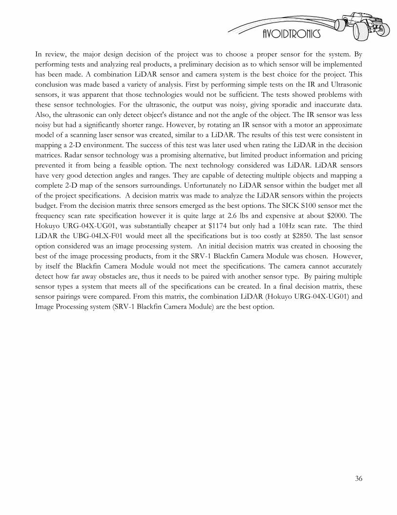
Table 3 Image processing sensor decision matrix
The Blackfin SRV-1 Camera module emerged as the dominant choice from the decision matrix. It
outperformed the other sensors in: Cost, Aesthetics, Power Requirements, Horizontal Range, and output
protocol. It was outperformed by at least one of the other sensors in: Impact Resistance, Resolution, and
CPU overhead.

34
3.2.4.5. Final Product Analysis
The decision matrix presented in Table 3 led to the selection of the Blackfin SRV-1 Camera Module as the
final image processing product.
Figure 30 Blackfin SRV-1 camera module
A brief description of the key features is presented below
Dimensions: 2.0” x 2.6”, 1.25 oz
3.6 mm lens, 90-deg view angle
1280x1024, 640x480, 320x256, or 160x128 pixel resolution
Onboard image processing
Built-in C interpreter
Direct support for 4 Sharp IR range finders

35
3.2.5. Final Decision Matrix
From the previous analysis there were no sensor systems that met the specifications outlined for the project.
The LiDAR sensors have many of the qualities needed, but the sensors within the budget are either too
heavy or do not meet the specified scan time. The image processing systems have the required scan time
but lack the required distance detection capabilities. The decision matrix below in Table 4, pairs multiple
sensor types, in hopes of creating a sensor system that meets the project specifications. Four different
systems are analyzed. The first is the UBG-04LX-F01 LiDAR (which was previously determined as too
expensive at $2850) is used as a reference for comparison. The second option is a Camera (Blackfin SRV-1)
and IR sensor. This would be the cheapest of the options but would require the IR to track the object which
could be difficult. The third is a Camera and LiDAR (Hokuyo URG-04LX-UG01) combination. The fourth
is a dual LiDAR system where the sensors would scan at asynchronous times in order to meet the 20Hz
scan rate. As seen in the table the highest scoring combination was the camera and LiDAR system. This
system can use the camera to detect obstacles between scans of the LiDAR. Conceivably this would raise
the scan frequency from 10Hz to the required 20Hz. This combination meets all of the specifications.
Table 4 Final Decision Matrix with Sensor Pairing
3.3. Conceptual Design Conclusion
36
In review, the major design decision of the project was to choose a proper sensor for the system. By
performing tests and analyzing real products, a preliminary decision as to which sensor will be implemented
has been made. A combination LiDAR sensor and camera system is the best choice for the project. This
conclusion was made based a variety of analysis. First by performing simple tests on the IR and Ultrasonic
sensors, it was apparent that those technologies would not be sufficient. The tests showed problems with
these sensor technologies. For the ultrasonic, the output was noisy, giving sporadic and inaccurate data.
Also, the ultrasonic can only detect object's distance and not the angle of the object. The IR sensor was less
noisy but had a significantly shorter range. However, by rotating an IR sensor with a motor an approximate
model of a scanning laser sensor was created, similar to a LiDAR. The results of this test were consistent in
mapping a 2-D environment. The success of this test was later used when rating the LiDAR in the decision
matrices. Radar sensor technology was a promising alternative, but limited product information and pricing
prevented it from being a feasible option. The next technology considered was LiDAR. LiDAR sensors
have very good detection angles and ranges. They are capable of detecting multiple objects and mapping a
complete 2-D map of the sensors surroundings. Unfortunately no LiDAR sensor within the budget met all
of the project specifications. A decision matrix was made to analyze the LiDAR sensors within the projects
budget. From the decision matrix three sensors emerged as the best options. The SICK S100 sensor met the
frequency scan rate specification however it is quite large at 2.6 lbs and expensive at about $2000. The
Hokuyo URG-04X-UG01, was substantially cheaper at $1174 but only had a 10Hz scan rate. The third
LiDAR the UBG-04LX-F01 would meet all the specifications but is too costly at $2850. The last sensor
option considered was an image processing system. An initial decision matrix was created in choosing the
best of the image processing products, from it the SRV-1 Blackfin Camera Module was chosen. However,
by itself the Blackfin Camera Module would not meet the specifications. The camera cannot accurately
detect how far away obstacles are, thus it needs to be paired with another sensor type. By pairing multiple
sensor types a system that meets all of the specifications can be created. In a final decision matrix, these
sensor pairings were compared. From this matrix, the combination LiDAR (Hokuyo URG-04X-UG01) and
Image Processing system (SRV-1 Blackfin Camera Module) are the best option.

37
Chapter 4. Final Design
The following diagram shows the high level data flow for the system. The subsystems’ logic, software, and
hardware will be discussed in detail in the following sections.
Figure 31. System overview showing the process flow of the system.
The system developed utilizes a 1/10th scale, two-wheel drive remote controlled car as the test platform.
Environmental data is collected using a Hokuyo UBG-04LX-F01 LiDAR sensor which is capable of
producing a scan of the environment 35 times per second. Using the data collected by the LiDAR obstacles
in the vicinity of the vehicle are parsed and identified as obstacles. The road cones are parsed separately
from the obstacles and are used to locate the boundaries of the road relative to the vehicle. After the road
boundaries and obstacles have been determined a threat coefficient is defined for each obstacle using the
estimated time to collision between the test vehicle and the obstacle. If the obstacle is outside of the road
or the test vehicle is not moving the threat is set to zero. If the threat coefficient for any of the detected
obstacles goes outside of the acceptable range the system engages autonomous control. When under
autonomous control the system uses the Rapidly Exploring Random Tree (RRT) path planning algorithm to
determine a safe path around the collision. The steering inputs needed to follow each segment of the path
are calculated with the path and checked against the physical limits of the test vehicle. Once a safe, feasible
path has been determined the steer commands are tuned by the non-linear, eight degree of freedom vehicle
model-predictive-stability controller to address any steer commands which may have caused rollover

38
conditions. The tuned steer commands are sent, via a hardwired connection, to the test vehicle, causing it to
follow the desired path.
In the final implementation of the code the MPC controller was removed from the loop due to inaccuracies
in the developed vehicle model. It is, however, and important part of the project development and will be
discussed in the following sections. Stability was achieved by tuning the maximum steer angle that the RRT
would allow.
4.1. Hardware Development
The following section details the development of the hardware used in this project
4.1.1. Final Sensor Selection
After the conceptual design review with the project sponsor the project’s budget was increased to allow for
the purchase of the Hokuyo UBG-04LX-F01 LiDAR sensor, which meets the project specifications. The
small, compact sensor has a notably fast scan rate of approximately 35 Hz. A complete specifications sheet
can be found in Appendix D. The single LiDAR sensor was selected as the primary sensor as it is much
easier to implement than the LiDAR and Camera combination discussed in the design development section
of this paper. Figure 32 below shows the LiDAR and some of its key specifications.
4.1.2. LiDAR Mounting Bracket Design
In order to secure the LiDAR to the vehicle chassis a mounting bracket was designed. The primary
considerations in the design of the mounting bracket were as follows:
Sensor must not be subjected to any forces, impacts, or accelerations that violate the design specifications of the sensor during normal test operations or foreseeable misuse
Sensor attitude must be able to adjust ±5 degrees from horizontal
Figure 32. Hokuyo UBG-04LX-F01

39
Sensor must be rigidly secured to the chassis such that there is no detectable relative motion during normal test operation
Mounting solution must use existing vehicle attach points when possible
Mounting solution may not interfere with the operation of any existing vehicle components
Mounting solution must allow access to the LiDAR
Mounting solution must be removable
Alterations of existing vehicle design should be minimal
The solution to the above cited design criteria includes the design of a mounting bracket that attaches to
existing chassis attach points, a protective casing, and a slight modification of the roll cage to accommodate
the mounting bracket.
Figure 33. Solid model including updated roll cage and LiDAR mounting bracket
Figure 564 shows a rendered image of the mounting bracket with the re-designed roll cage mounted on the
vehicle. The sensor is mounted forward on the vehicle so that there is less interference in the output data
from vehicle components.

40
Figure 34. Exploded view of LiDAR Mounting bracket
Figure 345 shows the mounting bracket with the LiDAR attached. The mounting bracket consists of six
individual components- including the LiDAR- Technical drawings of which are presented in Appendix O.
The standoff (1) uses the existing vehicle features to create a flat mounting surface for the base plate (3).
The angle aluminum mounting bracket (4) and the protective case (6) are then attached to the base plate,
securing and protecting the sensor. The 22 M3 Jam nuts (2) allow the attitude of the base plate to be
adjusted in three dimensions, meeting the requirement for adjustability. The protective case prevents
foreign objects from contacting the sensor as well as providing impact and vibration insulation via four 1/16
inch foam inserts. The angle support allows the LiDAR to be rigidly attached to the bracket. All of the
mounting bracket components will be created using 3D printing, allowing for the easy manufacturing of
complex geometries.
4.1.2.1. Mounting Bracket Analysis
The protective case and the roll cage protect the LiDAR from impact while the foam inserts in the
protective case provide vibrational damping for the LiDAR. In a crash scenario it would be possible for the
vehicle to experience high accelerations that would then be transmitted to the LiDAR sensor, possibly
exceeding the impact resistance rating of the sensor. The LiDAR is rated to withstand a 196 m/s2
accelerations 3 times each in the x, y, and z directions. In order to assure that the sensor would not
experience accelerations greater than this limit the vehicle accelerations were measured in a scaled crash test.
All sensitive electronic components were removed from the vehicle and an accelerometer was attached to
the chassis of the vehicle. The vehicle was then elevated and allowed to roll down an inclined ramp into a
wall.
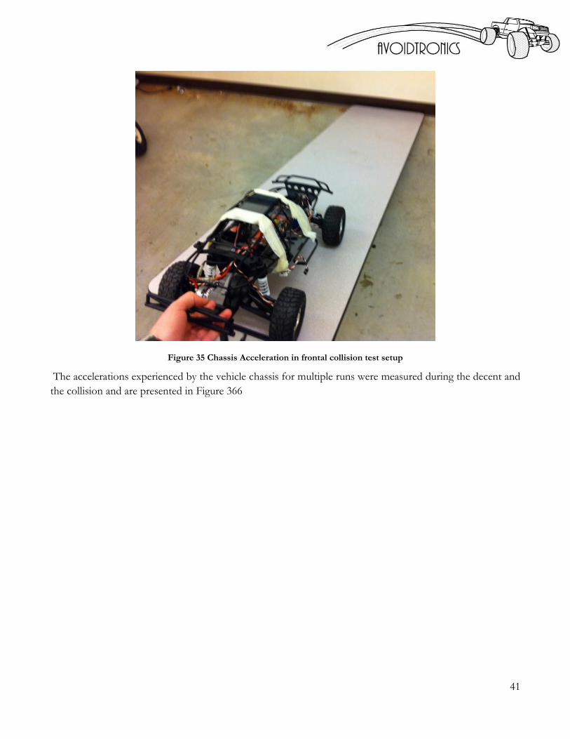
41
Figure 35 Chassis Acceleration in frontal collision test setup
The accelerations experienced by the vehicle chassis for multiple runs were measured during the decent and
the collision and are presented in Figure 366

42
Figure 36 Chassis acceleration as a function of time for the frontal collision setup shown in Figure 34
Using a trapezoidal approximation the vehicle speed was estimated prior to the collision. The average speed
of the vehicle prior to the collision was approximately 6.5 ft/s, less than the 10 ft/s test velocity. In order to
estimate the vehicle acceleration in a collision at full speed an energy scaling approach was selected. A
simplified energy analysis is presented below which shows that the kinetic energy of the vehicle is
transferred into spring potential energy of the bumper with some losses due to friction. Using the equations
below with the collected data the effective spring rate of the vehicle can be calculated
If it is assumed that Eloss other represents a constant proportion of the energy lost in a collision with the same
vehicle and that the bumper of the car does not reach full compression then a similitude equation can be
derived. This equation can be used to calculate the expected accelerations in a collision within a limited
velocity range around the test data.
(
)

43
The maximum acceleration of the vehicle during the three test runs was measured to be .972 g, this resulted
in an expected maximum acceleration of 2.27g in a full speed frontal collision. This is a full order of
magnitude lower than the acceptable limit for the sensor and therefore requires no further design
consideration.
4.1.3. Powering the LiDAR
To power the LiDAR four 3.7V Lithium-Ion batteries will replace the four AA batteries that were used by
the previous group. They will mount to the car in a similar and slightly larger four slot battery case. The new
batteries will have sufficient voltage to power both the LiDAR and the microcontroller based circuit boards.
A proposed schematic for regulating the 14.8-16.5V down to the appropriate voltages of 12V and 3.3V for
the LiDAR and the circuit boards, respectively, can be seen in Figure 37. This redesigned power supply
utilizes two voltage regulators and a simple voltage divider with filtering capacitors on both the input and
output of the regulators to smooth out any sudden current demands. A larger capacitor bank will be used to
filter noise and ripple from the battery supply before being regulated. Note that if an appropriate 3.3V
regulator is selected, it may not be necessary to use a voltage divider if the 3.3V regulator is specified for
such a voltage drop and excess heat dissipation is not a concern. Otherwise, selection of the two resistors
making up the voltage divider must be chosen to drop the voltage to a safe level for the regulator. The
voltage shall not be dropped below the minimum voltage input for each regulator, according to the
component’s datasheet.
Figure 37. Circuit diagram for LiDAR Power circuit

44
4.1.4. Data Acquisition from LiDAR
In order to relay the LiDAR sensor’s data back to the main computer the sensor’s USB connection is used.
The USB connection with an independent data tether to the computer was selected over the Serial
connection due to the much higher data transfer rate. The maximum rate of data transfer for serial
communication ports on a PC is 115 Kbit/s while the maximum rate of data transfer for USB 2.0 is 480
Mbit/s. The use of a 64 foot USB extension from the test vehicle to the computer reduces the actual data
transfer rates for the USB to USB 1.1 speeds of 12Mbit/s. With the LiDAR producing 726 data points per
scan and 35 scans per second it is not possible to transfer the data in real time via a serial connection but the
data is easily passed via USB.
The data sent over the USB connection is in an encrypted format to decrease the amount of data that is
passed in each scan. Information regarding the encryption and C code libraries needed to retrieve data from
the sensor can be found online.
4.1.5. IMU and Wheel Encoders
The Sparkfun 6-DOF IMU which existed from the work of the previous two groups is now used solely to
determine the roll rate of the vehicle. All other data that was collected from the IMU has been replaced
with data collected using the LiDAR sensor.
The wheel encoders are used to estimate the velocity of the vehicle but do not account for wheel slip or the
effects of cornering in the approximation.
The IMU and wheel encoders pass data to the slave PIC board which then passes the data to the master PIC
board. The master PIC board then transmits the serial data via the main data tether to the computer. For a
more detailed description of the PIC communication protocol please see “A MODEL PREDICTIVE
CONTROL APPROACH TO ROLL STABILITY OF A SCALED CRASH AVOIDANCE VEHICLE”
by Nikola Noxon.
4.1.6. Power Supply
The power supply underwent further revision for the final design. The final power supply offers more
features such as a wider range of DC supply rails (+3.3V, +5V,+12V) that use high efficiency DC-DC
switching voltage regulators, a low-battery indicator LED, an overload protection fuse, and an enable pin to
selectively toggle the output of each switching regulator with external hardware; this ideal for implementing
an emergency shut-down. It is vital that the batteries be changed once the low-battery indicator LED
(yellow) comes on; this indicates that the voltage provided by the cells has dropped below the threshold of
+14.7 volts. If the supplied voltage drops too low the boards that control the steering and throttle behavior
of the car will start to send and receive bad data that usually results in erratic behavior. In addition, changing
the batteries at the appropriate time helps to prevent from deep-discharge.
Please refer to the DC-DC switching power supply datasheets for the circuit and passive components used
with each regulator. The low battery indicator circuit consists of two NPN transistors, a trimmer, and a
resistor & LED. The trimmer can used to set the threshold voltage at which the LED comes on, currently
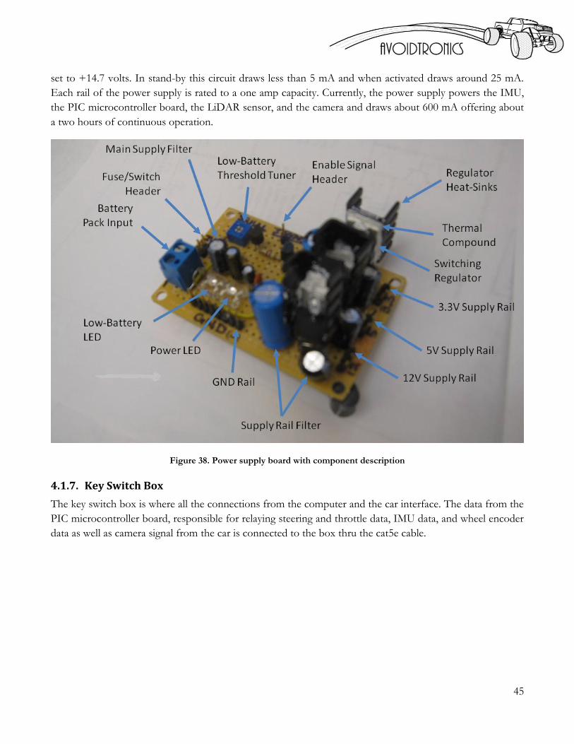
45
set to +14.7 volts. In stand-by this circuit draws less than 5 mA and when activated draws around 25 mA.
Each rail of the power supply is rated to a one amp capacity. Currently, the power supply powers the IMU,
the PIC microcontroller board, the LiDAR sensor, and the camera and draws about 600 mA offering about
a two hours of continuous operation.
Figure 38. Power supply board with component description
4.1.7. Key Switch Box
The key switch box is where all the connections from the computer and the car interface. The data from the
PIC microcontroller board, responsible for relaying steering and throttle data, IMU data, and wheel encoder
data as well as camera signal from the car is connected to the box thru the cat5e cable.

46
Figure 39. Key box with component labels
Upon coming into the box the cat5e cable connections are broken out with the video signal going to an
RCA connector, the toggle signal going to an Atmel microcontroller, and the other signals going to a serial
converter. An RS232 to USB serial converter FTDI board located within the switch box provides the
required voltage level and protocol conversions to enable the computer to communicate with the
microcontrollers. The Atmel microcontroller monitors the key position and provides a signal to the toggle
pin of the switching regulator that powers the PIC microcontroller board. The key provides an on/off
control to the boards that rely the steering and throttle data, which simultaneously provides an emergency
shut-down method; an LED light, located below the key, indicates the on/off status of the PIC board.

47
Figure 40. Inner wiring of Key box with component descriptions
4.1.8. User control
User control of the test vehicle is accomplished by use of a Logitec steering wheel and pedal controls. The
signal from the steering and pedal commands is interpreted by the Simulink code and passed through the
main data tether to the test vehicle.
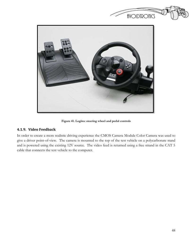
48
Figure 41. Logitec steering wheel and pedal controls
4.1.9. Video Feedback
In order to create a more realistic driving experience the CMOS Camera Module Color Camera was used to
give a driver point-of-view. The camera is mounted to the top of the test vehicle on a polycarbonate stand
and is powered using the existing 12V source. The video feed is returned using a free strand in the CAT 5
cable that connects the test vehicle to the computer.

49
4.2. Software Development
The top level Simulink block diagram for this system is shown in Figure 42. The primary segments of the
code include data collection from the LiDAR using Matlab’s C-MEX compiler, data parsing using Java, and
RRT path planning using Matlab. The MPC controller is not implemented in this version of the code.
Figure 42. System Simulink high level block diagram
Data is collected from the LiDAR Sensor (1) and is passed into the segmentation and threat determination
block (2) where it is parsed into obstacles and road boundaries. Simultaneously the IMU and Wheel
Encoder data is retrieved from the serial bus (3) and parsed to determine the vehicle speed. With the data
from all of the vehicle sensors the threat coefficient is determined (2) at set high if there is an imminent
collision detected. If no threat is detected the user’s steer and throttle commands (6) are passed to the
vehicle. If a threat is detected a safe path around the obstacle is developed by the RRT Algorithm (5). The
toggle between user and computer control is managed by a switch block with a built in function (7) acting as
an emergency kill if the “O” button on the steering wheel is pressed. The steer and throttle commands are
then sent across the data bus to the car using the COM port block (8)
4.2.1. LiDAR Data collection
The code used to retrieve data from the LiDAR sensor is based on the C libraries provided by Hokuyo and
available for download at http://www.hokuyo-aut.jp/02sensor/07scanner/download/products/ubg-04lx-
f01/. In order to integrate the C code into the Simulink environment Matlab’s MEX capabilities were used.
MEX allows C code to be compiled and run in the Matlab environment. For a detailed discussion of MEX
operation please see the User Manual in Appendix M. Construction of a custom Simulink S-function allows
the compiled C code to be run in Simulink.
4
1 2
5
6
4
3
7
8
7

50
The highest level function for the URG Library is GD_Scan. This file contains the C main() function as
well as the MEX gateway function. The file has three modes: Initialization, Data Collection, and Shutdown.
In the Initialization routine the code initializes a serial connection with the lidar using the pre-defined
commands
urg_initialize(&urg); ret = urg_connect(&urg, device, 115200);
A data structure that contains all of the connection information, data pointers and handle for the serial connection is defined and set as persistent using the MEXmakememorypersistant() command. The pointer to this data structure (URG_PTR) will be available for subsequent calls to the MEX file and allows the serial connection to remain open even though the MEX file closes. The laser is also turned on during initialization. In the data collection routine, the persistent URG_PTR is utilized to call the LiDAR’s “GD” routine, retrieving the most recent data scan from the buffer. This can result in scan times anywhere between .005 and .05 seconds depending on where in the scan the laser is when the routine is called. The command
urg_requestData(URG_ptr, URG_GD, URG_FIRST, URG_LAST)
Returns a 726x1 array of long data types representing the distance data collected by each beam. For a more detailed discussion of the function parameters please see the Hokuyo communication protocol on the manufacturer site In the Shutdown routine all data other than the URG_PTR created in the initialization routine is freed, the laser is set to idle, and the serial connection is terminated. The persistent URG_PTR will remain in memory until “clear mex” is called or Matlab is shutdown.
4.2.2. Segmentation
Once the data is attained from the LiDAR sensor via serial communication, the data is passed to the
segmentation algorithm in order to identify obstacles within the point-cloud and to determine their state.
The segmentation of detected obstacles within the point-cloud happens in three steps that occur in tandem:
point clustering, parsing each point cluster to obtain geometric properties, and obstacle tracking & velocity
estimation. In the first step, the segmentation algorithm first identifies obstacles by clustering adjacent
points in the point-cloud together to form discrete sets of ordered points, which make up each obstacle’s
definition. When to begin and when to end an obstacle definition, or cluster of ordered points, is controlled
by various parameters, which subsequently control the size and location of the bounding boxes (detected
obstacles). To generate bounding boxes around obstacles detected within the point-cloud, the clustered
points making up each obstacle definition are parsed using the cluster-method algorithm. The output of the
segmentation process is the state of each detected obstacle, including its position, size, and velocity.
Parameters control the aspects of how points are clustered; these parameters include the max number of
points, max step size, min area, and a scaling factor. A description of each parameter is as follows:
Threshold distance: This parameter controls how far to look for obstacles surrounding the car.

51
Max Number of Points: This parameter controls the maximum number of points that can be clustered
together for each obstacle definition.
Max Step Size: This parameter controls when to end an obstacle definition. If adjacent points within
the point-cloud are greater than the max step size and are both within the threshold
distance while the max number of points has not yet been reached the definition ends.
This allows for obstacles placed near each other or near to walls can be identified
and segmented separately.
Min Length: This parameter, determined dynamically as the detected distance multiplied by the
angular resolution, controls the minimum width and/or length each detected
obstacle may possess. This will avoid any plane surface obstacle detected from
having an infinitesimal length or width value.
Scaling Factor: This parameter controls how much each detected object is to be scaled by and is
used to slightly buffer each detected obstacle’s geometry before path-planning.
Max Velocity: This parameter filters any obstacle velocity estimations that are not feasible, typically
occurring with points that fall off either side of the obstacle’s definition over time.
Figure 43. egmented Point-Cloud Results and the Actual Test Layout
To cluster points within the point-cloud, the algorithm iterates through the data starting at the first index
and moving the last while a temporary buffer holds the current obstacle definition. Upon iteration, if the
current point is at a distance less than the threshold distance it is added to the current obstacle definition. If
either the max number of points or the step difference is exceeded then the current obstacle definition is ended,
processed, and a new detected obstacle is added to a set holding all detected obstacles. Finally, the buffer is
cleared. In addition, if the current point is outside the threshold, but the previous point was inside the
threshold the same occurs; the obstacle is also processed, added, and cleared.

52
Every time the end of an obstacle definition is identified, the points within the definition are processed and
the result contains the state of the detected obstacle, which is added to a large set of all detected obstacles.
The cluster-method algorithm processes each obstacle definition, or set of points, to attain the geometric
information (location and size) of each detected obstacle; by simply using the maximum and minimum x
and y values in the each cluster of points within the definition, the bounding box and centroid can be
determined.
In order to estimate the velocity of each obstacle they must be tracked through time or the points making
up each obstacle definition must be tracked through time. This algorithm estimates each detected obstacle’s
velocity by calculating the change in position of each point making up the obstacle definition over time,
between iterations. Since the number of points in each obstacle definition change through time this method
allows it so the same obstacle with different definitions to be compared easily at different times. Keeping
the points ordered in the point-cloud allow for easy obstacle tracking as each has a unique index and will
always be adjacent to other points within the obstacle definition. A velocity accumulator calculates each
point’s change in position over time within the obstacle definition and divides by the total number of points
to estimate each obstacle’s velocity. The first and last points of the obstacle definition are ignored as these
are fall off points; these points fall off the obstacle definition over time and are ignored because they
produce impossibly large velocity estimations. In addition, the contribution of each point to the velocity
estimation is checked against the max velocity expected to filter out any other fall off points. Due to the
change in position, namely translation and rotation, of the car over time, the previous point-cloud must be
brought to the current reference frame in order for this estimation to work. This means that the previous
point-cloud must be translated and rotated in order to line up the points to the current point-cloud and
match the beam indices. Once the road is detected and the yaw rate is determined the number of indices to
rotate the previous point-cloud by can be calculated; the distance to translate is calculated by the speed of
the car, given by the wheel encoders, multiplied by the time between iterations. The previous point-cloud
cloud is translated point-by-point and rotated point-by-point using a rotation transformation matrix
allowing to check the change in position of each point in the obstacle definition by referencing the index
number (beam number). It can be noted that obstacles with a smaller number of points in their obstacle
definition with which to estimate their velocity will have greater error.
4.2.3. Road Detection
Currently, accurately and reliably identifying the road bounds is a critical facet in determining system
performance. The car’s yaw is currently calculated by determining the slope of the road using the LiDAR
sensor alone. In addition, the path-planning algorithm requires roadway input parameters in order to
function properly. As of now, the algorithm determines the road bounds by identifying the location of two
traffic cones, both on the same side, in order to calculate the slope intercept of the road line characterizing
that side of the roadway. The other side of the roadway can be calculating by offsetting the road line by the
known road width in the proper direction. This means for the road to be detected two traffic cones must be
identified out of the detected obstacle array, while ensuring they are on the same side of the car.
After the point-cloud data is segmented, a set of detected obstacles exists that contains each obstacle’s
location as well as the width, length, and velocity components. This set of obstacles is further segmented in

53
order to differentiate traffic cone obstacles from other obstacles and to identify the road bounds. Once the
all the traffic cones are identified in the detected obstacle list, a new list containing the road bound obstacles
is created and the original list is trimmed of the road cone obstacles. The road cone obstacle list is then
parsed to obtain the actual road boundaries. These boundaries are used to threatening obstacles within the
roadway, whether traveling off the roadway is imminent, as well as dictating the bounds the car must stay
within during an avoidance maneuver. A description of each parameter controlling the road detection
algorithm is as follows:
Road Width: This parameter should reflect the actual road width of the test track and controls the offset
when calculating the unknown road line.
Cone Spacing: This parameter should reflect the actual cone spacing used on the test track and controls
what spacing to look for when identifying cone obstacles within the set of detected
obstacles.
Spacing Buffer: This parameter controls the buffer on the detected cone spacing when comparing it to the
expected cone spacing when differentiating between obstacles.
Area Threshold: This parameter controls the area expected to be detected by a traffic cone obstacle (from
segmentation) and is used to differentiate road cones obstacles and other obstacles.
Minimum Area: This parameter controls the minimum area expected to be detected during segmentation by a
traffic cone obstacle.
Area Buffer: This parameter controls the buffer on the detected area of an obstacle when comparing it to
the area threshold for road cone identification.
Round Bound Offset: This parameter controls the inwards offset of the road lines from the detected road
bounds acts as a road detection buffer.
Max Slope Change: This parameter filters out any falsely identified road bounds, which occurs when the
previous slope and the new of the road bounds difference is greater than the max slope
change conceivable.

54
Figure 44. Road detection. Note detected obstacles within the roadway and the inwards from of road lines from the line
of cones within the point-cloud.
Once the LiDAR point-cloud is segmented, the set containing the detected obstacles is further processed to
parse out road cone obstacles and to identify the road roads. A first pass iterates through the set of detected
obstacles and calculates the detected area, searching for areas that match the area threshold with respect to the
area buffer; if there is a match the obstacle is added to a set of possible road cones for further consideration.
After the possible traffic cones are identified the spacing between each possible cone obstacle is compared
to the actual cone spacing used on the test track. If the spacing between the possible cones matches the cone
spacing within the spacing buffer, two cones are identified; each cone is added to a set containing all the
identified traffic cones that define the road bounds. After all cones within the set of possible cone obstacles
have been identified and added to the set of identified traffic cones, any duplicates are removed. In addition,
all the detected cones are removed from the original set containing all the detected obstacles that is output
after segmentation.
Once all the traffic cones have been identified, the set containing them is analyzed to calculate the road
bounds and to build the array that will be passed to the path-planning algorithm. This set is iterated through
until two cones can be identified on the right or left side of the car, which is done by checking whether the x
coordinate has a positive or negative value. When two cones have been identified on either side, the
iterations cease and the line’s properties describing the road boundaries are calculated (slope, intercept). To
ensure that the cones are identified on the same side of the car the detected cone spacing is once again
compared to the actual cone spacing to check the max slope change. With the orientation of the road lines
known, the car’s yaw angle with the respect to the road is calculated. Due to the trig functions that appear in
these calculations the car’s yaw angle is never allowed to be zero and rather is set to infinitesimal value when

55
appropriate. Finally, all the detected obstacles, in the detected obstacle set, that are located outside the road
bounds are removed.
If the road bounds cannot be found successfully, either because not enough cones could be identified or the
road slope changed dramatically, the previous road bounds are used. When the road cannot successfully be
identified a numerous times, successively the system will trigger a flag that sets the car to neutral. This acts
as a stop routine for when the car reaches the end of the test track. Even if this routine is mistakenly
triggered during a system maneuver there exists a chance to correct upon the next iteration when obstacles,
road bounds, and the threat to the car is reevaluated. Implementing more complex solvers may also allow
road detection by detecting only one cone on each side.
4.2.4. Threat Determination & User to Autonomous Toggle
Once a set of obstacles are identified that are within the road bounds, they are processed to deem if they
pose a threat of an imminent collision. If any obstacle within the set is deemed to be a threat to the car, it is
added to a set of threatening obstacles, which is used in the path-planning subsystem. If any threatening
obstacle is detected the toggle between user and autonomous control is enabled by setting the toggle high.
To determine whether each detected obstacle is to be deemed a threat or not, several parameters and
strategies are implemented; however, these are not by any means exhaustive. A description of each
parameter is as follows:
Minimum Speed: This parameter controls the minimum speed of the car below which no detected obstacle is
deemed threatening and hence the user will remain in control. This parameter aims to
prevent the system from engaging in scaled low-speed situations often encountered while
driving such as in a car park.
Minimum Distance: This parameter controls the minimum distance of the car to an obstacle which within no
threat is considered threatening and the reasoning mirrors that of the minimum speed
parameter. Note this parameter may be disabled by setting it equal to zero.
Threshold Distance: This parameter controls the minimum distance of the car to a detected obstacle within the
roadway and aids in determining if detected obstacles within the roadway are to be deemed
threatening.
Threat Cone Angle: This parameter controls the angle (+/-) of a cone projected in front of the car and aids in
determining if detected obstacles within the roadway are to be deemed threatening.
Previous Toggle: This parameter is always set to the previous toggle to help ensure that the system the switch
back to user control occurs in a safe manner, after a maneuver has been executed.
Threat Threshold: This parameter controls the threshold value of the threat coefficient that will trigger
autonomous control. The value is calculated as the inverse of the time to collision for each
detected obstacle within the roadway

56
Allowable Distance to Road Bound & Threshold Maneuver Angle: This parameter controls the allowable distance to
the road bounds at the threshold maneuver angle that will trigger autonomous control to prevent
traveling off of the roadway.
After segmentation and road detection has occurred, the set of detected obstacles that are within the
roadway can be processed according to these parameters to build a set of threatening obstacles to pass to
the path-planning subsystem and to determine whether the car is under user-control or autonomous control.
If the vehicle is not traveling at least the minimum speed no obstacles will be deemed threatening and the
toggle will not engage the system. However, if the car exceeds the minimum speed the threat of each obstacle
within the detected obstacle set will be determined. A detected obstacle is deemed threatening and added to
the set of threatening obstacles if: it is further than the minimum distance, it is within plus or minus the threat
cone angle, and the threat coefficient is greater than the threat threshold or the obstacle is within the threshold
distance. While an obstacle is added to the threatening obstacle set, the toggle will be triggered if not already.
After all detected obstacles have been deemed a threat or not, the distance to each road bound is calculated
and compared to the allowable distance to road bounds and the threshold maneuver angle to determine the danger of
leaving the roadway. Outside of this loop the toggle can also be triggered independently depending on the
previous toggle state to prevent giving user back control while executing an avoidance maneuver.
4.2.5. Simulation of Data Parsing and Road detection
In order to test the algorithms developed for the segmentation of the LiDAR’s point-cloud data and road
detection, a simulation was written in the java programming language to graphically show the results in real-
time. The user can use the keyboard arrow keys to command the car to move and turn while rectangular
obstacles pass by. While the user drives the car, a point-cloud of data is generated, to simulate the LiDAR
sensor’s data, every couple of milliseconds by casting out lines and detecting the intersection points with the
rectangular obstacles. Slight noise was added to the simulated data with a pseudo-random number generator.
Circular cone obstacles are drawn on the sides of the road to provide testing of the road detection
algorithm. An animation loop keeps the graphics up to date providing the motion of the car and obstacles as
well as the visual feedback of how well the segmentation algorithms are performing. In particular, the
current and previous point-cloud is shown as well as the detected obstacles and their velocity vectors. The
green circle surrounding the car represents the threshold distance, under which obstacles will be segmented
and a line for each beam of the LiDAR is drawn for visualization.
This simulation not only helped to verify the algorithm while simultaneously writing the code to be
implemented, but it helped to identify issues that were not foreseen and saved time when compared to
testing each sub-system on the real car with actual hardware. Not to mention this helped protect the
hardware from damage from the testing process. For example, initially it was believed that the difference of
circle and rectangles could be detected with the LiDAR sensor and then used to identify the road
boundaries. However, the LiDAR data is not ideal and even with the relatively high resolution the difference
between the two shapes could not reliably be identified. This was verified by the simulation, see Figure 45
when no noise was present the two shapes could be differentiated, however, simulating a small amount of
noise in the data showed this method would not work for road detection. Another observation is that the
estimated velocity vectors always point radially towards or away from the car using this algorithm and

57
obstacles defined with smaller number of points will produce greater error in the estimations of their
velocity, see Figure 45.
The java programming language was used due to the numerous data types and data handling APIs offered.
In addition, Matlab and Simlink allow direct implementation and use of java objects and classes that can be
packaged into Matlab S-functions. During testing, certain files written in the Matlab programming language
were found to run too slowly, namely the threat determination code, and were ported to the java language;
the code with the exact same function ran several orders of magnitude faster once ported. This is believed
to be because Matlab is a higher level programming language with more processing overhead than java.
Figure 45. Segmentation simulation screen shots

58
4.2.6. Rapidly Exploring Random Tree (RRT)
The following section describes the overall functionality of this implementation of the RRT algorithm as
well as highlighting changes from the previous group’s work
4.2.6.1. Coordinate System
With the addition of the sensor, it is advantageous for the system's coordinate system to be attached to the
front of the car at the LiDAR. This new coordinate system is shown in Figure 46. The LiDAR based
coordinate system makes much more sense as the car doesn't need to keep track of where it is relative to a
fixed global coordinate system. The car only needs to keep track of where the obstacles and road are relative
to the car. A comparison between the two coordinate systems is shown in Table 5. In order to convert the
system to a LiDAR based coordinate system many updates are needed to the RRT code. The largest changes
stem from how the road, goal, and vehicle state are handled. The road and goal in the global coordinate
system do not change as the car moves. However, with the LiDAR coordinate system these values will
change as the car moves down the road. Also, with this change in coordinate system the x,y position of the
car is not necessary as the car always lies at (0,0) relative to the LiDAR. Thus, with this new coordinate
system the vehicle position data gathered from the IMU is not needed for path planning. The changes made
to the RRT to switch from the global to LiDAR based coordinate system are outlined in more detail in the
following sections.
Figure 46. LiDAR and Global Coordinate System
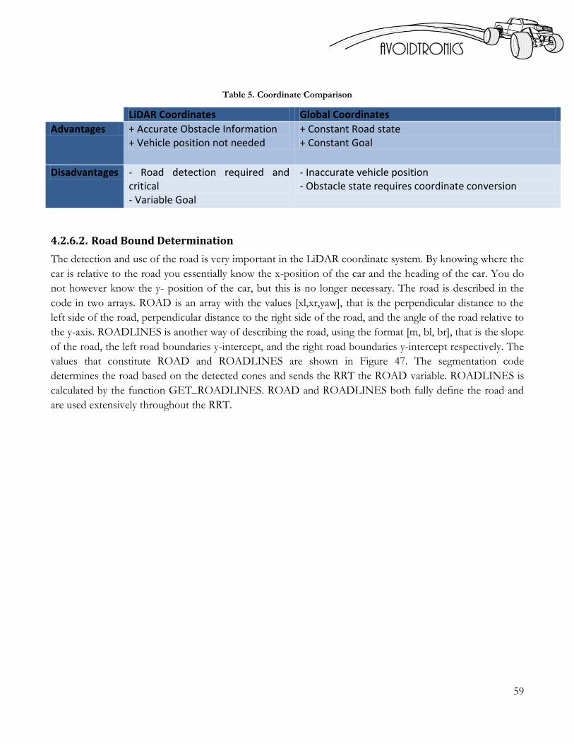
59
Table 5. Coordinate Comparison
LiDAR Coordinates Global Coordinates
Advantages + Accurate Obstacle Information + Vehicle position not needed
+ Constant Road state + Constant Goal
Disadvantages - Road detection required and critical - Variable Goal
- Inaccurate vehicle position - Obstacle state requires coordinate conversion
4.2.6.2. Road Bound Determination
The detection and use of the road is very important in the LiDAR coordinate system. By knowing where the
car is relative to the road you essentially know the x-position of the car and the heading of the car. You do
not however know the y- position of the car, but this is no longer necessary. The road is described in the
code in two arrays. ROAD is an array with the values [xl,xr,yaw], that is the perpendicular distance to the
left side of the road, perpendicular distance to the right side of the road, and the angle of the road relative to
the y-axis. ROADLINES is another way of describing the road, using the format [m, bl, br], that is the slope
of the road, the left road boundaries y-intercept, and the right road boundaries y-intercept respectively. The
values that constitute ROAD and ROADLINES are shown in Figure 47. The segmentation code
determines the road based on the detected cones and sends the RRT the ROAD variable. ROADLINES is
calculated by the function GET_ROADLINES. ROAD and ROADLINES both fully define the road and
are used extensively throughout the RRT.

60
Figure 47 ROAD and ROADLINES variables
4.2.6.3. Goal Determination
In the global coordinate system defining the goal was relatively easy. The goal was just defined as a distance,
Y, down the road and in the middle of the road (0,Y). With the LiDAR coordinate system the goal must be
defined differently. It is still a point some distance down the road, however since the road is not always
straight, the point will have an x-position other than zero. The goal is determined in the function
GET_GOAL which requires ROAD and ROADLINES as inputs. The new goal is calculated by finding the
equation of the line down the center of the road. Then using a user defined distance, GOAL_DIST, as the
hypotenuse to a right triangle, a Y-value for the goal is determined. This value is plugged into the center line
equation of the road and a X-value is found. The goal is then (X.Y). In this new method each time the RRT
runs a new goal is calculated.
4.2.6.4. Select Random Node
RAND_NODE is a random node that is cast out in front of the car and is used in the path planning. The
area in which this random point is cast should be within the road bounds. Thus, this new search space is in
the shape of a parallelogram, see Figure 48. To find this new RAND_NODE value, a line parallel to the
road, but within the road boundaries is found. Then a random point along that line is found and this
becomes the coordinates of RAND_NODE. This method guarantees that RAND_NODE is within the
road boundaries and is randomly found. To calculate this value, first a lower and upper limit on the y-

61
distance are set. This creates the top horizontal lines of a parallelogram. The road boundaries create the the
other sides to the parallelogram. A random value is selected using the "rand" function in MATLAB, on the
x-axis with the road bounds as the upper and lower limits. A random point is then selected on the y-axis in-
between the range specified by the max and min y-values, this will be used as the Y value of
RAND_NODE. Then using the random x-value as the x-intercept, a line is generated having the same slope
as the road. Plugging in Y into this equation and solving for the x-value, yields the x-coordinate of
RAND_NODE.
Figure 48 Geometry of RAND_NODE
4.2.6.5. Check for Collision
The CHECK_COLLSION function determines whether the RRT planned path violates the road
boundaries or hits an obstacle. With variable road boundaries the code was updated such that it checks the
vertices of the car against an angled road. This is accomplished by finding the y-values of the road at the x-
coordinates of all the vertices of the car. These eight points are kept in the array Y_max and Y_min. Then
the y-values of the vertices of the car are checked against Y_max and Y_min. If they are not between their
respective Y_max and Y_min values the road bounds the NOGOGO flag is triggered and the path is
terminated. A visual of the geometry is shown below in Figure 49.

62
Figure 49 CHECK_COLLISION visual
4.2.6.6. Multiple Obstacle Behavior
It is also important to note that with a LiDAR sensor multiple objects can be detected. This allows for path
planning around more than one obstacle. With this new feature the code needed to be updated to allow for
multiple obstacle detection. A simple while loop was placed around the CHECK_COLLISION function.
Allowing the code to run CHECK_COLLISION for each detected obstacle. If the planned path hits one of
the obstacles then the while loop is immediately terminated and a new path is planned.
4.2.7. MPC
For a discussion of the MPC’s implementation throughout this project please see “A MODEL
PREDICTIVE CONTROL APPROACH TO ROLL STABILITY OF A SCALED CRASH
AVOIDANCE VEHICLE” by Nikola Noxon
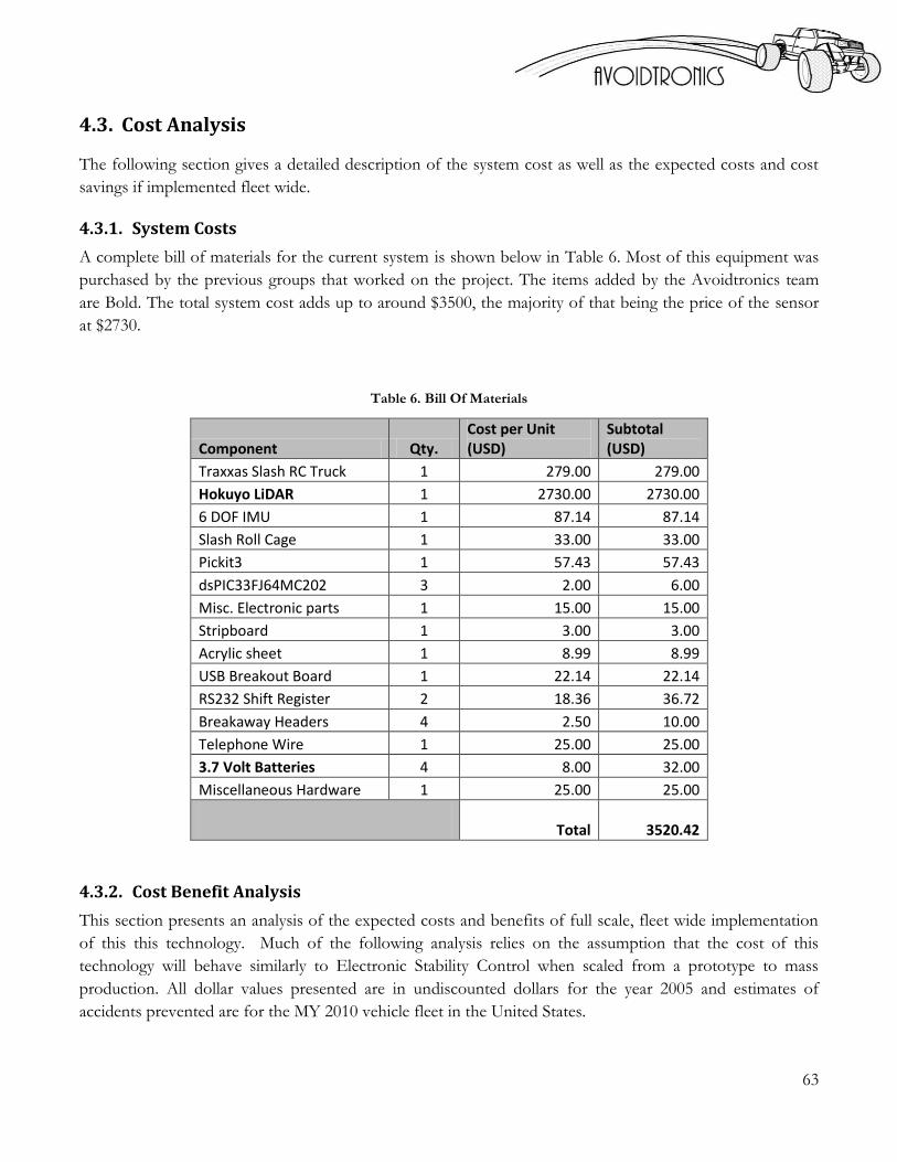
63
4.3. Cost Analysis
The following section gives a detailed description of the system cost as well as the expected costs and cost
savings if implemented fleet wide.
4.3.1. System Costs
A complete bill of materials for the current system is shown below in Table 6. Most of this equipment was
purchased by the previous groups that worked on the project. The items added by the Avoidtronics team
are Bold. The total system cost adds up to around $3500, the majority of that being the price of the sensor
at $2730.
Table 6. Bill Of Materials
Component Qty. Cost per Unit (USD)
Subtotal (USD)
Traxxas Slash RC Truck 1 279.00 279.00
Hokuyo LiDAR 1 2730.00 2730.00
6 DOF IMU 1 87.14 87.14
Slash Roll Cage 1 33.00 33.00
Pickit3 1 57.43 57.43
dsPIC33FJ64MC202 3 2.00 6.00
Misc. Electronic parts 1 15.00 15.00
Stripboard 1 3.00 3.00
Acrylic sheet 1 8.99 8.99
USB Breakout Board 1 22.14 22.14
RS232 Shift Register 2 18.36 36.72
Breakaway Headers 4 2.50 10.00
Telephone Wire 1 25.00 25.00
3.7 Volt Batteries 4 8.00 32.00
Miscellaneous Hardware 1 25.00 25.00
Total 3520.42
4.3.2. Cost Benefit Analysis
This section presents an analysis of the expected costs and benefits of full scale, fleet wide implementation
of this this technology. Much of the following analysis relies on the assumption that the cost of this
technology will behave similarly to Electronic Stability Control when scaled from a prototype to mass
production. All dollar values presented are in undiscounted dollars for the year 2005 and estimates of
accidents prevented are for the MY 2010 vehicle fleet in the United States.

64
If we assume that the target market for implementation of this technology is similar to that of Electronic
stability Control, i.e. passenger cars (PC) and light trucks (LTV) we can calculate the yearly cost benefit of
implementing this technology as:
4.3.2.1. Incremental Costs
In scaling this project to a full scale vehicle, many of the components presented in Table 6 could be
integrated into existing vehicle systems. The primary cost consideration would continue to be the LiDAR
sensor. If it is assumed that the same sensor were implemented in the full scale vehicle and that mass
production of and advances in LiDAR technology reduce the cost of the sensor by 80% (this is a
conservative assumption as the cost of an entry level LiDAR sensor has decreased by approximately 75% in
the last 3 years) then the incremental cost per vehicle in the fleet would be approximately $550. The
number of vehicles produced in 2011 in the United States was approximately 3 million.
4.3.2.2. Accidents Prevented
Estimates of the number and type of accidents preventable by this system are based on the “NTHSA 2010
Highway safety facts.” In order to accurately assess the cost benefits of this system, the 54 million police
reported accidents in 2010 must be limited to frontal collisions that could have been prevented by
autonomous steering. Table 7 shows the number of crashes in 2010 by crash type.

65
Table 7. Crashes by first Harmful Event, Manner of Collision and Crash Severity
Exclusion of rear end collisions, all non-collision accidents, and all “collisions with fixed objects” -as they
occur most often off the roadway- yields the correct target population of accidents for all vehicles. The
results of this simplification are given in Table 8

66
Table 8 Preventable Crashes by first Harmful Event, Manner of Collision and Crash Severity
The analysis must be further limited by vehicle type to include only Passenger Cars and Light trucks.
Table 9. Vehicles involved in Crashes by vehicle type and crash severity
Table 9 gives the vehicles involved in each crash type by vehicle type and can be used as a basis for further
analysis. If we make the assumption that the percentage of passenger cars and light trucks involved in each
accident type applied uniformly to the accidents presented in Table 8 we can fully develop the target
population of accidents using

67
The results of the above calculation are shown in Table 10
Table 10 Preventable Crashes by first Harmful Event, Manner of Collision and Crash Severity For Passenger cars and
Light Trucks
The table presented above represents a system effectiveness of 100% which is not a realistic assumption.
Further analysis will be conducted with an effectiveness rate of 50%, similar to that of Electronic Stability
Control.
4.3.2.3. Damages per accident
In order to fully define a monetary cost benefit for the implementation of the system it is necessary to
calculate not only the savings from property damages and travel delay, but also to ascertain the financial
implications of an injury or fatality. Table 11 gives the National Highway Traffic and Safety Administration’s
definition of the financial loss due to travel delay and property damage by MAIS injury severity.
Table 11 Financial loss due to travel delay and property damage by MAIS injury level
Table 12 gives the estimated comprehensive cost savings from reducing fatalities as published by the
National Highway Traffic and Safety Administration

68
Table 12. Calculation of Fatla Equivalents NHTSA Values
Due to a lack of published data it must be assumed that the accidents causing injury in Table 10 are evenly
divided amongst the MAIS 1-5 injuries. This assumption could be greatly improved by finding a correlation
between the number of injuries and the percentage of injuries in each MAIS severity level. On the basis of
this assumption we find that, combined with the number of accidents prevented the savings due to
implementation of this system is in the hundreds of billions of dollars.
Table 13 Total Savings of fleet wide system integration

69
Chapter 5. Design Verification
The following section describes the testing procedure used to validate the design as well as the results of
said testing. Autonomous
5.1. Testing Procedures
To ensure the system functions suitably the specifications outlined in Table 1 must be tested. A complete
test plan can be found in Appendix N. The test plan was developed to test the most important aspects of
the system and to verify that the project meets the specifications that were agreed upon with the sponsor.
Below is a more complete description of the tests in the test plan.
Battery Swap Time: This test will be performed to ensure that if a battery runs out of power it will be able to
be replaced in a reasonable time. The tester will time how long it takes to replace all the batteries on the car.
Required Equipment: stop watch
Battery Lifetime: During the ESV convention, the system may need to be running for long periods of time. It
is important that the lifetime of each battery pack be known, so that appropriate replacement batteries can
be purchased. The tester will run the system from fully charged and record the time it takes for the battery
to completely discharge. Required Equipment: stop watch
Sensor Range: One of the important specifications of the LiDAR is its range. The range is how far away and
how close the sensor can detect. The test will be performed by putting different objects at different
distances away from the LiDAR and seeing which it senses and which are out of its range. Required
Equipment: measuring tape.
Sensor Viewing Angle: It is essential that the LiDAR has a viewing angle of at least 54 degrees from the front
of the car. This is to ensure that it sees all objects that could cause frontal collisions. To find the viewing
angle objects will be placed around the sensor at different angles and a maximum viewing angle will be
recorded. Required Equipment: protractor
Sensor Scan Speed: The LiDAR must have a frequency of at least 20 Hz to match the frequency of the Matlab
code. This will be tested by collecting data from the LiDAR in real time then recording the frequency of the
acquisition.
Detected Obstacle Size: An obstacle will be placed in the sensing range of the car. The sensor will detect the
object then run the data through the code. The obstacle size that is determined from the sensor and sensor
processing code will then be compared to the actual size of the object. The two areas must be within 20% of
each other for a passing test. Three different obstacles with different sizes will be tested at three different
locations. Required Equipment: measuring tape
Detected Obstacle Location: An obstacle will be placed 3ft and 7ft away from the car. The obstacle location will
be determined from the sensor. Then the distance between the detected obstacle and actual obstacle will be

70
determined. This distance must be less than 2 inch at 3ft away and less than 4 inches at 7ft away. Required
Equipment: measuring tape
Detected Obstacle Velocity: A moving obstacle will be placed in front of the sensor. The sensor will detect the
object then run the data through the code; the code will determine the obstacles velocity. This velocity will
be compared to the actual velocity which will be found by knowing the distance the obstacle travels in a
certain time. Required Equipment: measuring tape, stopwatch
Maneuver Speed: The car is supposed to simulate crash avoidance at freeway type speeds. Therefore at a 1/10
scale the car should be able to perform its maneuvers at a speed of 6.81 mph, which scaled is 68.1 mph. To
test this, a maneuver will be performed at the systems max speed. The tester will record the distance the car
travels and the time of the maneuver to determine the maneuver speed. Required Equipment: measuring
tape, stopwatch
Repeatability: With the implemented sensor the car should successfully avoid the three collision scenarios
completed by the previous group. They are avoiding a stationary car, a car that starts stationary then moves
away, and lastly a moving car. The car should be able to avoid collision in all three of these scenarios with a
95% success rate. Required Equipment: obstacle car, road barriers
Driver Satisfaction Survey: The purpose of this test is to quantify the public’s reaction to an autonomous crash
avoidance system. The test will have participants drive the car towards an imminent collision then have the
car’s systems take over and avoid the obstacle. A survey will be provided to the driver after the test and the
driver will indicate whether they were satisfied with the technology or if it was unsatisfactory. Eighty percent
of the participants must be satisfied to for a passing test and at least 30 participants must be surveyed.
Avoid Two Static Obstacles: The purpose of this test is evaluating the system behavior with multiple obstacles
in the roadway. Two boxes will be placed in the roadway and the car will be driven directly at one of the
boxes, activating the avoidance system. The system should be able to avoid collisions with an 80% success
rate.

71
5.1.1. Testing Results
The results of the tests described in the Design Validation section of this report are presented below as well
as pictures of the test setup and additional descriptions where applicable.
Table 14. Final Subsystem testing results
The results of the initial sub-system testing are presented in Table 14 above. The detected obstacle size and
detected obstacle velocity were outside of the specifications range.
The detected obstacle size being out of range is due to the fact that with a single, 2D scanner it is impossible
to estimate the size of a box oriented so that the sensor can only see a planar face of the box. If the box is
oriented so that a corner and two sides can be seen the algorithm approximates the size of the obstacle
within 10%. Figure 50 below shows a scan of two boxes and the detected obstacles. In this setup the two
boxes were oriented so that the lidar could only see the planar surface of the boxes.
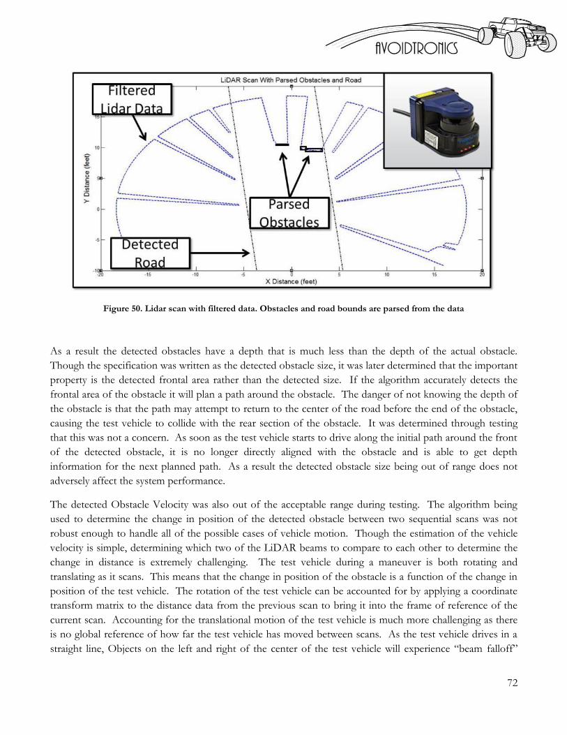
72
Figure 50. Lidar scan with filtered data. Obstacles and road bounds are parsed from the data
As a result the detected obstacles have a depth that is much less than the depth of the actual obstacle.
Though the specification was written as the detected obstacle size, it was later determined that the important
property is the detected frontal area rather than the detected size. If the algorithm accurately detects the
frontal area of the obstacle it will plan a path around the obstacle. The danger of not knowing the depth of
the obstacle is that the path may attempt to return to the center of the road before the end of the obstacle,
causing the test vehicle to collide with the rear section of the obstacle. It was determined through testing
that this was not a concern. As soon as the test vehicle starts to drive along the initial path around the front
of the detected obstacle, it is no longer directly aligned with the obstacle and is able to get depth
information for the next planned path. As a result the detected obstacle size being out of range does not
adversely affect the system performance.
The detected Obstacle Velocity was also out of the acceptable range during testing. The algorithm being
used to determine the change in position of the detected obstacle between two sequential scans was not
robust enough to handle all of the possible cases of vehicle motion. Though the estimation of the vehicle
velocity is simple, determining which two of the LiDAR beams to compare to each other to determine the
change in distance is extremely challenging. The test vehicle during a maneuver is both rotating and
translating as it scans. This means that the change in position of the obstacle is a function of the change in
position of the test vehicle. The rotation of the test vehicle can be accounted for by applying a coordinate
transform matrix to the distance data from the previous scan to bring it into the frame of reference of the
current scan. Accounting for the translational motion of the test vehicle is much more challenging as there
is no global reference of how far the test vehicle has moved between scans. As the test vehicle drives in a
straight line, Objects on the left and right of the center of the test vehicle will experience “beam falloff”

73
where a beam that was initially on the object may fall off the edge of the object due to the forward motion
of the test vehicle. This results in the object in that beam having an apparent velocity even if the object is
not moving. Due to inaccurate velocity estimates it was predicted that the test vehicle would not be able to
consistently avoid moving obstacles. Due to time restraints it was decided that full system testing should be
conducted even though the velocity estimation was inaccurate. This effectively limits the scope of the
system to static obstacles or obstacles that are moving very slowly. In the case of an obstacle that is moving
very slowly the high frequency with which new paths are planned is sufficient to avoid the obstacle.
Potential solutions to this problem are presented in the Future Work section of this report.
It was determined that full system testing could be conducted, even though the Detected Obstacle Size and
Detected Obstacle Velocity were not within the specified ranges. The testing for the Repeatability criteria
was conducted by setting up a test track and testing the system twenty times for each of the three scenarios.
The same test setup was used for the driver satisfaction survey and is shown in the figure below. In the
single static obstacle test, a single box was placed in the center of the test track. In the static obstacle moves
away at the last second test a single obstacle was placed in the center of the road and then moved off of the
road to the right when it was 5 feet from the test vehicle. In the moving obstacle test as single obstacle was
driven across the road from right to left across the path of the test vehicle. The two static obstacle test was
similar to the single static obstacle test with an obstacle in the center of the road, but with a second obstacle
5 ft behind and to the left of the first obstacle. The two static obstacle test and the test setup for all of the
other scenarios is shown in Figure 51
Figure 51. Experimental setup for reliability test and driver satisfaction survey
The results of the Repeatability testing are shown in Table 15.

74
Table 15. Results from repeatability testing as well as the two obstacle test
The results of the full system testing did not meet the specifications set out at the onset of this project
except for the system’s ability to avoid two static obstacles.
The requirement for the Single Static Obstacle avoidance was set at 95% in the project specifications.
During testing the system was actually able to avoid collisions in 80% of the test runs. The test setup for
the single obstacle avoidance case was similar to the test setup described above, however only one obstacle
was place in the center of the road. It would seem that the single obstacle test is the simplest case of all;
however an analysis of the system architecture showed that this is not the case. In each of the failed runs
the data from the LiDAR, the segmentation, the RRT and all other subsystems were stored and analyzed. It
was discovered that the primary reason that the system failed was due to the random nature of the RRT
algorithm. With the obstacle placed in the center of the road, there is the same number of viable paths on
the left hand side of the obstacle as there are on the right hand side of the obstacle. This results in
successive paths being planned, one to the right and one to the left. While both left and right are valid
paths, the steer commands issued by the first path were counteracted by the steer commands for the second
path. This resulted in the test vehicle driving almost perfectly straight down the road until a collision was
unavoidable and the RRT Algorithm failed. When the RRT failed, the system continues to read the steer
commands previously issued and attempts to follow the last path set out by the RRT. If the RRT failed far
enough obstacle, the car would none the less avoid the obstacle. If the RRT failed too close to the obstacle,
or did not fail at all, the car would continue straight towards the obstacle with perhaps one desperate
maneuver at the last second.
The requirement for the Static Obstacle Moves Away at Last Second test was set at 95% in the project
specifications. During testing the system was actually able to avoid collisions in 90% of the test runs. The
test setup for the static obstacle moves away at last second test is identical to the single static obstacle test
with the exception that the obstacle drives out of the path of the vehicle. When the test vehicle is 5 feet
away from the obstacle the obstacle begins to drive off the road to the right. Surprisingly, the system was
able to more consistently avoid the obstacle in this test than in the static obstacle test. A review of the data
showed that when the system initially engaged these tests were subject to the same left-right toggling as the
single static obstacle test. As the obstacle moved off of the road, it reduced the number of viable paths on
the right side of the obstacle while increasing the number of viable paths on the left side of the obstacle. As

75
a result, after the first 2-3 iterations the RRT would tend to plan paths to the left of the obstacle. With
multiple consecutive paths being planned to the left of the obstacle the test vehicle would more consistently
avoid the obstacle. The cases where the test vehicle did not successfully avoid the obstacle were caused
either by the system being unable to identify the road boundaries during a maneuver or from the RRT
planning a path in the direction of the moving obstacle before failing. In the case were the system was
unable to properly identify the road boundaries it was noticed that in some runs the RRT would never-the-
less produce a path. This path would attempt to drive the vehicle along a road that could be 90 degrees
rotated from the actual orientation of the road. As a result the RRT would produce steer commands that
caused the test vehicle to drive erratically. Subsequent scans may have produced correct road boundaries
and valid paths; however the interjection of near random steer commands would often cause the system to
fail. Updates to the code needed to fix the issues causing erratic road behavior are discussed in the future
work section of this report.
The requirement for the moving obstacle avoidance was set at 95% in the project specifications. During
testing the system was actually able to avoid collisions in 50% of the test runs. After testing of the velocity
estimation algorithm, it was not expected that the system would be able to avoid moving obstacles
consistently. With the moving obstacle going from left to right, the system was able to avoid a collision only
in situations where the first 2-3 paths were planned to the left of the vehicle. Without accurate velocity
estimation, the system would plan paths into the way of the moving obstacle as often as it would plan paths
away from the moving obstacle. With a system frequency of 20Hz it was anticipated that the test vehicle
would be able to avoid a moving obstacle in more than 50% of the cases, however this was not the case.
Updates to the code required improving the velocity estimation and therefore the ability to avoid moving
obstacles is discussed in the future work section of this report.
5.1.2. Driver Satisfaction Survey
A copy of the driver satisfaction survey with the result from testing is presented in Appendix I . The result
of a small selection of the questions and their interpretation are discussed in this section. It should be noted
that the demographic of people who were involved in the system testing is Mechanical Engineering students
and faculty at Cal Poly and my not accurately represent the opinion of the general public.
Figure 52. Question from driver satisfaction survey with results

76
Every participant was asked if they thought that autonomous collision avoidance systems have the potential
to save lives. 100% of the people asked agreed that this technology has the potential to save lives. This
indicates that when the technology is mature people will be more likely to consider it on their vehicle if they
think that it could save their life someday
Figure 53. Question from driver satisfaction survey with results
26% of the survey participants said that they would absolutely trust a vehicle with autonomous collision
avoidance technologies and 67% of the participants said that they would possibly trust this technology. This
was an interesting contradiction to the fact that the majority of participants thought that the largest
roadblock to implementation of this technology is driver’s perceptions of the technology.
Figure 54. Question from driver satisfaction survey with results
This question shows that, for our test demographic, the overwhelming majority of the participants would
feel safer driving a vehicle with an autonomous collision avoidance technology than a similar vehicle
without.
It was discovered after reviewing the survey data that very few conclusions could be drawn regarding a
change in perception caused by the test. The survey questions asked did not align such that a distinct
change in opinion could be measured. As a result the data was used primarily as information regarding the
survey participant’s inclinations regarding autonomous vehicle technology in general.

77
Chapter 6. Conclusions and Future Work
In this section the conclusions will be presented with the future work needed to fix known issue or improve
system performance.
6.1. Conclusion
After the national level presentation the team was selected to compete at the Enhanced Safety of Vehicles
international student design competition in Seoul, South Korea. The team placed first at the international
competition. Despite winning the international competition, the system did not perform to the
specifications set up at the start of the project. Many of the major issues that led to substandard system
performance have been documented and are discussed in the future work section of the report. The system
was unable to avoid moving obstacle consistently due to the inaccuracies in the velocity estimation. There
were also issues associated with running the RRT algorithm at a high frequency such as the system
oscillating between paths to the left and then to the right of the obstacle. The LiDAR based obstacle
detection and segmentation of the detected obstacles works very well and will continue to be an integral part
of this project throughout further development. Issues involving the consistent detection of the road
boundaries led to some system failures and will need to be improved in future iterations of the project.
6.2. Future Work/Recommendations
Obstacle Identification– Implementing another sensor, using the existing camera, and or implementing a
more robust algorithm, possibly utilizing edge detection or color detection, can not only allow for
obstacle differentiation, which can be used to bias and more accurately determine the threat to the
system improving user perception and avoiding false user to autonomous toggle while also
dramatically increasing the road detection performance.
Update and Improve Velocity Estimation & Obstacle Tracking – As of now the velocity vectors produced
from the segmentation and tracking algorithm are always radially pointed towards or away from the
vehicle. This makes them useless for path-planning, but adequate for conservative threat coefficient
determination. Once this issue is addressed, the system should avoid moving obstacles significantly
better.
Implement Camera for Road Detection - Use of the existing camera in tandem with the LiDAR data will
make road detection easier. This update alone should allow for near perfect static obstacle
avoidance.
Optimized Path-Planning Algorithm - Would eliminate the pitfall of the current system, which has
extreme difficulty committing to a direction when faced with a sole obstacle centered in the
roadway; so much so that the system often fails. This update would include checking the previously
planned path and determining if a new path is needed. If the old path is still a valid path an new
78
path should not be planned and the test vehicle should be allowed to continue following the
previously issued steer commands.
User To Autonomous Control Toggle - As of now, when the system is turned on the toggle is initialized
to user control. Upon detection of any threatening obstacles the system engages and the toggle turns
on. Once the threat are safely avoided and passed the system toggle is set to neutral and will remain
so until the system is turned off and restarted, It is trivial to have the system return to user control
once the threats are safely passed, however, the test track was not long enough to justify this. In
addition, the threat determination and toggle to autonomous control was sensitive during testing,
but improvements are expected if obstacle road detection is improved and obstacle identification is
implemented.
Throttle/Brake Control - Implement throttle/brake control in the control loop in addition to steering
control. This would allow for determining whether the safest maneuver is steering control, braking,
or a combination of the two.
On-board Processing – Doing the processing onboard will increase the frequency at which the system
can operate. It will also remove the physical tether to the computer which will make the system
more aesthetically pleasing
C Code Memory Leak – In its current implementation the MEX code that connects to the LiDAR and
collects data leaks memory. A memory leak is when memory is set aside for a variable and is never
cleared. This results in Matlab bogging down the computer after 2-3 runs of the system and needing
to be restarted. Updating this memory leak should help improve system performance as the
machine operating the code will have more available RAM.
IMU Data Filtering - Implement a Kalman filter to be able to detect the yaw of the car accurately and
either use alone or compare to yaw determined from the road detected with the LiDAR sensor. It
would be most beneficial, in terms of processing, accuracy, and reliability, to use the IMU for yaw
determination instead of the LiDAR. This would allow the road detection using the LiDAR alone to
not be as critical, which currently is a major pitfall.
Simulation – Can be extended to simulate the path-planning, threat determination, and autonomous
control of the actual system and may serve as a stepping stone for on-board processing. This could
also save time testing the system in simulation to catch some errors that may otherwise take longer
to identify running sub-system or full-system tests on the actual system. More realistic acceleration
and turning algorithm could also be implemented to better simulate the car and obstacle dynamics.

79
Appendix A Quality Function Deployment

80

81
Appendix B Specifications Sample Calculations
Horizontal Viewing Angle
Figure 55 Required Viewing Angle for Full View of Wheel-Base 12 inches from Front Bumper
Sensor Size
Figure 56 Sensor Size and Available Space Comparison

82
Appendix C Prototype Car Code
This code was used to sample and process Ultrasonic, IR, and LiDAR data during testing. The code was
developed for an Arduino board.

83
Arduino (Atmega32) Sketch

84
Appendix D Hokuyo UBG-04LX-F01 Scanning Laser Rangefinder

85

86

87

88

89

90
Appendix E CMOS Camera Module Color Camera Spec Sheet

91

92

93

94
Appendix F LM 2592HV SIMPLE SWITCHER specification Sheet
For a complete specification sheet please see the Manufacturer site or the Dropbox/Data Sheets

95
Appendix G Gannt Chart
See Dropbox/Administrative/Schedule

96
Appendix H ATMEL ATtiny 13A Micro controller specification sheet
For Complete Data Sheet please see Dropbox/Data Sheets

97
Appendix I Driver satisfaction survey and results
Thank you for participating in the Autonomous Vehicle Technology Survey being conducted by California Polytechnic State University’s Advanced Vehicle Collision Avoidance team. The survey is a combination of multiple-choice and short-answer questions and takes approximately 10-15 minutes to complete. Definition of Autonomous Vehicle: For the purposes of this survey, we define an autonomous vehicle as one that can self-navigate and pilot without human intervention using advanced technologies such as sensors, actuators, vehicle-to-vehicle and vehicle-to-infrastructure communication, etc. We also recognize that autonomy may come in varying degrees, from selective use (e.g., parking assist) to continuous autonomous operation. ------------------------------------------------------------------------------------------------------------------------------------------------------------------------------------------------------------------------------------------------------------------------------------
1. In your view, how soon will fully autonomous vehicles be capable of reliable operation on public streets? a. The technology is ready now (11%) b. Less than 5 years (19%) c. In 5 to 10 years (22%) d. In 10 to 25 years (37%) e. More than 25 years (7%) f. Never (4%)
2. Do you think that autonomous collision avoidance systems have the potential to save lives? a. Yes (100%) b. No (0%)
3. Would you trust a production vehicle equipped with an autonomous collision avoidance system?
a. Absolutely (26%) b. Marginally (67%) c. Definitely not (7%) (please explain) ________________________________________________________
4. Would you consider purchasing a vehicle with a certified autonomous collision avoidance system? a. Definitely would (22%) b. Probably would (52%) c. Definitely would not (11%) d. Depends (please explain)_____(15%)_____________________________________
5. I would feel safer driving in a production vehicle with a certified autonomous collision avoidance system
than in a vehicle without one. a. True (70%) b. False (30%)

98
6. In your opinion, how much would a consumer buying a luxury vehicle be willing to pay for an autonomous collision avoidance system?
a. Less than $500 (0%) b. Between $500 and $1000 (0%) c. Between $1000 and $2000 (37%) d. More than $2000 (59%) e. No one would ever buy it (0%)
7. Would you be more likely to buy a vehicle with an autonomous collision avoidance system if the initial
cost was offset by savings on your insurance rates? a. Yes (78%) b. No (0%) c. Maybe (22%)
8. Which of the following would most likely make you think that a vehicle with an autonomous collision avoidance system is safer than a vehicle without one?
a. Acceptance and implementation by a large car manufacturer (15%) b. Certification by the National Traffic Highway and Safety Administration (26%) c. A live demonstration of the technology (33%) d. A recommendation from a friend (0%) e. I already think that these vehicles are safer (11%) f. Other(Please explain) ___________________________________________ (0%)
9. Do you think people would drive more recklessly if their vehicle had a collision avoidance system?
a. Definitely (22%) b. Probably (19%) c. Possibly (37%) d. Unlikely (22%) e. No (0%)
10. While driving on the freeway a driver initiates a lane change into an unsafe situation where they may or
may not have been able to avoid a collision. During the lane change their Certified autonomous collision avoidance system activates and steers them out of the unsafe situation, but during the maneuver side-swipes a nearby vehicle. Who should be liable for the property damage?
(select all that apply)
a. The vehicle manufacturer (4%) b. The supplier that provided the component hardware or software (11%) c. The driver (30%) d. federal government (0%) e. The entity that certified the vehicle for autonomous driving mode (if one exists) (4%) f. The driver's insurance (7%) g. Other (please specify)________________________________________________
STOP Do not complete this until after the demonstration

99
1. Did the car avoid the obstacles? a. Yes (95%) b. No (5%)
2. During the avoidance maneuver did you feel: (select all that apply)
a. Surprised (37%) b. Comfortable (4%) c. Scared (0%) d. Confused (11%) e. Relieved (7%) f. No Feeling (4%) g. Other (please explain) _ ______(7%)______________________________________
3. After driving this vehicle you _____________ purchase a vehicle with autonomous technology (as
compared during the first portion of the survey) a. Definitely would (15%) b. Probably would (48%) c. Probably would not (11%) d. Depends (Please explain)_____(19%)______________________________________
4. Do you think that autonomous collision avoidance systems have the potential to save lives?
a. Yes (100%) b. No (0%)
5. After driving this vehicle, would you trust a vehicle equipped with an autonomous collision avoidance
system? a. Absolutely (26%) b. Marginally (67%) c. Definitely not (4%) (please explain)_________________________________________________________
6. After driving this vehicle, how comfortable would you feel riding in a vehicle with an autonomous collision avoidance system?
a. Very Comfortable (19%) b. Comfortable (63%) c. Not Comfortable (15%) d. I would never ride in one of these vehicles (0%)
7. Do you think a fully autonomous vehicles will ever be safer and more reliable than human drivers? If so
by what year. a. Yes (15%) b. No (30%)
Year________________ (2030 average)

100
8. What do you think the biggest hurdle car manufacturer's face in trying to create and implement
autonomous vehicles? a. Consumer perceptions/bias (30%) b. Technological capabilities (4%) c. Financial reasons (15%) d. Government regulations (0%) e. Liability issues (22%) f. Other (Please Explain) ____________________________________________________
9. Imagine you are a CEO of a large car manufacturer how much of your R&D budget would you allocate
towards autonomous vehicle systems? a. <5% (15%) b. 5-10% (48%) c. 10-25% (30%) d. 25-40% (4%) e. >40% (0%)
10. What improvements could be made to the system you drove today to make the experience more
enjoyable:

101
Appendix J GD_Scan code (abbreviated)
For a complete version of the code please see dropbox/Working System/URG \example md_scan.c \brief Sample of MD scan Get the distance data of specified number of times using MD command. \author Satofumi KAMIMURA $Id: md_scan.c 1989 2012-05-18 00:32:36Z satofumi $ */ #include "urg_ctrl.h" #include <stdio.h> #include <stdlib.h> #include <assert.h> #include <math.h> #include "mex.h" struct coords { double* yptr; double* xptr; }; /* declared global to allow for the use of the mexmakepersistant command*/ static urg_t *URG_ptr = NULL; void exitFcn() { if (URG_ptr != NULL) urg_laserOff(URG_ptr); urg_disconnect(URG_ptr); mxFree(URG_ptr);} /* Handles exiting in case of an error state while connecting */ static void urg_exit(urg_t *urg, const char *message) { printf("%s: %s\n", message, urg_error(urg)); urg_disconnect(urg); free(URG_ptr); #ifdef MSC getchar(); #endif exit(1);} /* Start of the initialization routine, Urg data structure is stored for *later calls to the function*/ void main(void) { enum { CaptureTimes = 1, }; /* Define COM port, should be dynamic in future development */ const char device[] = "COM12"; /* For Windows */

102
Appendix K Java Segmentation Code (abbreviated)
For a complete version of the code please see dropbox/Working System/LiDar processing Class
import java.util.ArrayList; // Import data collection handling library for datatype arraylist import java.util.*; // Import data collection handling library for datatype hashset import static java.lang.Math.*; // Import library for common math functions public class ClusterMethodWithFinal { // Global Variable Initialization private ArrayList<double[]> AllObstacles = new ArrayList<double[]>(); // Store all current obstacles private ArrayList<double[]> ThreateningObstacles = new ArrayList<double[]>(); // Store all current threatening obstacles private ArrayList<double[]> Obstacle = new ArrayList<double[]>(); // Discrete group obstacle constructor private ArrayList<double[]> VelocityObstacleChk = new ArrayList<double[]>(); private ArrayList<double[]> RoadPts = new ArrayList<double[]>(); // Road bounds private ArrayList<Integer> PossibleRoadPts = new ArrayList<Integer>(); // Possible road bound indexes from detected obstacles private ArrayList<Integer> toRemove = new ArrayList<Integer>(); // Remove identified road bounds from detected obstacles private int Threshold = 50; // Threshold distance value in feet (Obstacles and road boundaries determined within this range) // Note: can rewrite to identify and determine road boundaries even outside of this threshold (max sensor range) private int maxNumPts = 10; // Max points allowed for point clustering when forming discrete groups representative of obstacles and boundaries private double MaxVelocity = 10.0; // Twice the max anticipated velocity in ft/s (relative terms - max velocity possible) private double ScalingFactor = 1; // Scaling factor, % (Buffer) private double angularRes_rad = 0.36*(PI/180); // LiDAR sensor's angular resolution in radians private int beamnumber = 726; // Default value - set dynamically to the length of the point-cloud array (below) private double areamin = 0.001; // Cone area min. for road detection private int noRoadCount = 0; // Current # of successive no road bounds private boolean noRoadFlag = false; // Current no road bound flag - set ea. iteration private double[] roadBounds = {0,0,0,0,0,0}; // Road bounds [-d_l,d_r,yaw,m,b_l,b_r] private double[] prevRoadBounds = {0,0,0,0,0,0}; // Previous road bounds [-d_l,d_r,yaw,m,b_l,b_r] private double prevRoadSlope= 0; // Previous slope of road bounds private double deltaYaw = 0; // Change in yaw (determines if car has turned)

103
Appendix L RUN_RRT code (abbreviated)
For a complete version of the code please see dropbox/Working System/RRT function FINAL_PATH = RUN_RRT(VEHICLE, OBSTACLE_ARRAY, ROAD)
%BEGINNING OF SIMULINK BLOCK*******************************
TEMP_NODE= zeros(3); %[x,y,cn] TREE=zeros(500, 3); %[x,y,cn] ROUTE_TREE=zeros(400,2);%[x,y] PATH=zeros(50,5); %[x,y,theta,delta,t,r] NODE_DIST=5; DONE=0; NODES=1; RAND_GO=0; TREE=zeros(500,3); FINAL_TREE=zeros(20,2); %EC: Don't need this TREE(1,1:2)=VEHICLE(1:2); %EC: Don't need this TREE(1,3)=0; FAIL=0; ITERATIONS=0; VEHICLE_GEO_ACTUAL = [22/12 1]; BUFFER = .5; VEHICLE_GEO=VEHICLE_GEO_ACTUAL+BUFFER; %[length,width] FINAL_PATH=zeros(50,5); %arbitrary size
%Trimming Function index = find(OBSTACLE_ARRAY(:,1),1,'last'); % Find the first 0 in array OBSTACLE_ARRAY = OBSTACLE_ARRAY(1:index+1,:); % Trim array to that index SIZE=size(OBSTACLE_ARRAY); %OBSTACLE array size ONumber = SIZE(1); %Number of Obstacles
% no road detected if ~any(ROAD) FAIL = 1; end
% Road aligned along car axis if ROAD(3) == 0 ROAD(3) = 0.00000001; end
%GET LINES OF ROAD BOUNDARIES ROADLINES = GET_ROADLINES(ROAD); %ROADLINES = [slope,left y-intercept, right y-
intercept]
%GET GOAL GOAL = GET_GOAL(ROAD,ROADLINES);
while (DONE==0 && FAIL==0) NOGOGO=0; %ADD A TEMPORARY NODE TO [TREE]

104
Appendix M System Operation Manual
Setting up The System
Setting up the Software
Computer with Matlab 2010b or higher
Microsoft Visual C++ Redistributable 2008 or higher with Windows SDK 6.1
a. Windows SDK 7.1
OR
b. Microsoft Visual C++ Redistributable 2008 or higher with Windows SDK 6.1
AND
c. Install the latest java runtime environment (JRE), however, it is recommended that you install the latest
java development kit (JDK) should you need to update the segmentation code and recompile it. See
oracle’s website for more details.
http://www.oracle.com/technetwork/java/javase/downloads/index.html
The exact software required depends on which version of MATLAB you have, and if you are running a
32bit or 64bit computer. You must set the MATLAB compiler to C++ using the MATLAB command
“mex –setup”. Select the C++ 2008 or 2010 compiler form the list of available options. See the following
for more details:
http://www.mathworks.com/support/compilers/R2012a/win64.html
http://www.mathworks.com/help/techdoc/ref/mex.html
To run the RSC/RRT program, see the “MATLAB Documentation for Roll Stability Control” in the
MATLAB sub-folder.
Onboard Control Unit Programming
The following is required to program the onboard control unit
1. Onboard control unit
2. PICkit3 with USB cable

105
3. MPLAB IDE
MPLAB IDE can be found for free on their website at:
http://www.microchip.com/stellent/idcplg?IdcService=SS_GET_PAGE&nodeId=1406&dDocNa
me=en019469&part=SW007002
To program using the PICKit3, see the following documentation:
http://www.sparkfun.com/datasheets/Programmers/PICkit_3_User_Guide_51795A.pdf
There are three folders containing the full code for each MCU. “picware” is an old file, which assumes that
one MCU runs the onboard control unit (OCU). This could be used in the future if a new control unit using
a larger, faster dsPIC, was installed. “picware 2” contains the code for MCU1 that communicates with the
computer and controls the throttle/steering. “picware 3” contains the code for MCU2 that gathers the IMU
data, and sends it back to MCU1. The MCUs split responsibility for gathering encoder data.
Setting up the Hardware
To setup the hardware:
Begin by turning on and opening a computer equipped with the proper version of Matlab and with
the proper compilers and supporting software installed.
Setup the steering wheel and foot pedals by plugging them into both power and a free USB port on
the computer.
Next plug in the TV monitor to the key switch box to the RCA connector and power.
Take the 100’ cat5e cable and connect one end to the car and the other to the key box.
Attach the LiDAR sensor with the 65’ USB cable to the computer.
Attach the key box to the computer with an USB A-to-micro cable.
Replacing the Li-Battery Pack Cells:
The Li-Battery has a PCB protection board as a safety feature and requires that the board be reset each time the batteries are replaced. No voltage will appear across the battery pack’s terminals after replacing the batteries until the PCB board is reset. To reset the PCB board apply a voltage of around 12-16VDC with another source, connecting the ground signals and power signals together for a brief time; just a few seconds is sufficient:
Disconnect the fuse and master switch jumper wire from the header marked FUSE on the
power supply.

106
Replace the dead Li-cells with newly charged Li-cells.
Obtain a voltage source of around 12-16 VDC.
Connect the ground of the battery pack to the ground on the source and the power from
the source to the positive terminal of the battery pack. This is most easily accessible by
touching the wires to the screws of the terminal block itself.
Test the voltage across the terminal block or battery pack.
If no voltage appears repeat the above process.
Reconnect the fuse and switch to the header on the power supply to reconnect all hardware
components.
Running the System
To run the full system:
Ensure that the hardware and software setup has been performed.
Open the Simulink model MPC_gamecontroller_LiDAR.mdl in the RRT folder.
Ensure the COM ports for the key box match the hardware reference in the Simulink model with
the device manager. Check that the Lidar COM port matches the COM port in the gd_scan file (see
updating LiDAR code below)
Verify all connections and battery conditions.
Turn the key on the switch box to the OFF position.
Turn on the master switch on the front of the car and make sure the LiDAR sensor turns on and
blinks green and the camera view is visible on the TV monitor.
Next turn on switch on the PIC microcontroller boards to the on position. Nothing will happen if
the key on the key switch box is in the OFF position.
Now turn the motor controller on by pressing the button, the LED on should be solid green. If not
please refer to the troubleshooting portion below.
Now turn the key on the switch box to the ON position. The LED on the switch box and the LED
on the motor controller should be solid red.
The system is ready to start: press the play button in the Simulink model. If not started soon after
turning all the hardware on the motor controller may go idle in which case refer to the
troubleshooting section below.
After initialization and calibration routines are done the user will be in control and able to drive
down the test track with autonomous control taking over once a threat is detected until after the
obstacles are passed, when the system will turn to neutral.
To run the LiDAR sensor sub-system:
To run the segmentation sub-system:

107
After running the LiDAR subsystem or loading previously saved data, open any of the road testing
Simulink models such as RoadTestingFinalVersionWitThreat.mdl
Change model parameters in the start-up callback method
Click RUN
To run the path-planning sub-system:
open MAIN_BLOCK_V1 in the RRT folder
change the road, obstacle, and vehicle speed to desired values
Click RUN
NOTE: this will only run one iteration of the RRT and plan only one path
Plotting Data outputs from a run: After the run open “RoadBounds and Obstacle Plotter.m” and run this file To run the LiDAR from the command line:
Make sure that it is powered on and connected to the computer
Check that the COM Port is set correctly
Type “gd_scan(0)” in the command line to connect
Type “[x y] = gd_scan(1)” to collect data
Type “gd_scan(2)” to disconnect
Updating the Software
LiDAR C Code: The LiDAR Code will need to be updated to match the COM port that the LiDAR is plugged into on the computer. This will be different for each machine that it is plugged into, so it will be good practice to do this before running the system. To Update the COM port in the code or to make any other changes:
Make sure that the C compiler is installed and set up as described above
From Matlab Open the file titled gd_scan (in the URG folder)
Check the COM port in the device manager (Control Panel)
Update the name of the COM port in the code (line 57 if nothing has changed)
/* Define COM port, should be dynamic in future development */
const char device[] = "COM12"; /* For Windows */
Save the file
Make sure that the Current folder is URG in matlab
In the matlab command line compile the code using the following command: o mex -output gd_scan -v *.c
Find the compiled MEX file (gd_scan.mex) and copy it into the RRT file

108
Java Segmentation Code
Ensure that the latest version of the java development kit (JDK) from Oracle is installed. To compile the
java code into classes that are usable within Matlab and Simulink, files must be compiled with the correct
version of java, version 1.6. The command to perform this compilation can be issued from the command
line with a computer, installed with the java development kit (JDK), located in the same folder. The
command line can be located and opened by finding an application called ‘command prompt.’ The
compilation command will produce a (.class) file that can be implemented in Matlab and Simulink by placing
the file in the appropriate place, or the RRT folder. There is a callback function in the Simulink model that
constructs the class for use while running at every model start time; the end callback function also clears the
java class at model end time. Note when java objects are initialized/constructed they clear the objects in the
workspace so they must be initialized prior to initializing any other object, such as the object used to
communicate with the LiDAR (gd_scan). See start-up and end functions from the Simulink model callbacks.
To compile:
Open Command Prompt (Windows) or Terminal Application (Mac and Linux)
Navigate the command line to the folder containing the java file to be compiled. Note you will
start in the root directory.
The command ‘dir’ (Windows) or ‘ls’ (Mac and Linux) lists the contents of the current directory. The command ‘cd’ stands for change directory.
Keep using the ‘dir’ (Windows) or ‘ls’ (Mac and Linux) to list the contents of the current directory and then use ‘cd directoryToNavigate2’ until you are in the directory with the (.java) file to be compiled. Note if you need to go back a directory in the directory tree type ‘cd ..’ into the command line.
Once in the correct folder compile by typing the following into the command line.
‘javac –source 1.6 –target 1.6 NameofJavaFileToCompile.java’ Note that if you are recompiling any files for the java segmentation simulation the –source 1.6 –
target 1.6 is not required.
‘javac NameofJavaFileToCompile.java’
If no errors appear, place the file now with (.class) into the dRRT folder so the Simulink
model start-up callback method can find the class.
Updating the Hardware
Power Supply
The power supply was designed to be somewhat future-proof by offering multiple high-efficiency supply
rails each boosting a 1 A current draw capacity and powered by a pack of Li-cells to provide long life and

109
hopefully will need minimal modifications. It should be noted that the 5V switching regulator was
disconnected and disabled because, during testing, the feedback loop of regulator was shorted causing
damage that resulted in strange behavior in the output power when under load. If the 5V rail is desired to be
used in the future a replacement switching regulator should be installed, as well as the supporting passive
components. Please refer to regulator datasheets for further information.
Switch Key Box
The emergency switch, while cutting throttle to the car will also lock the wheels in one direction as the
It may be desired to update the switch key box wiring, for example, splicing the video signal to provide both
a connection to a TV monitor and the computer for image processing. These updates can be performed by
opening the box, gently, by removing the faceplate attached with four machine screws. The Amtel ATtiny
13A microcontroller that monitors the position of the switch can also be updated or expanded to include
features, such as a remote controlled shut-down via a TV remote and an IR sensor. See datasheet, existing
AVR and Arduino code folder, as well as well-supported online community resources.
Troubleshooting
If the motor controller LED is blinking green turn off the master switch and restart the system from
the start of the running the system portion above. Another option is to turn off the motor controller
and PIC microcontroller board and reset them in the order specified in the running the system
portion above.
If Matlab crashes due to a error referencing an unknown state check the LiDAR sensor connections
and try to establish connection from the Matlab command line by typing gd_scan(0). If no errors are
reported the connection is successful, disconnect with gd_scan(2). Note gd_scan(1) will return a
single scan’s data from the LiDAR sensor
If Matlab gives an error referencing a COM communication problem, check the COM ports in the
device manager and ensure that they match the ports referenced in the Simulink model for each
piece of hardware.
If the toggle never engages the system when there is an apparent threat ensure that wheel encoder
data is being received. If not, check the wheel encoders’ continuity.
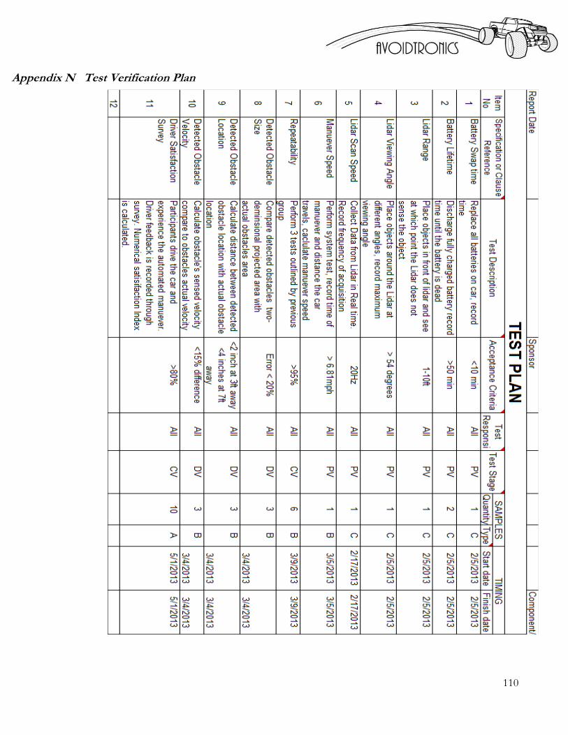
110
Appendix N Test Verification Plan

111
Appendix O LiDAR Mounting Bracket Technical Drawings

112

113

114
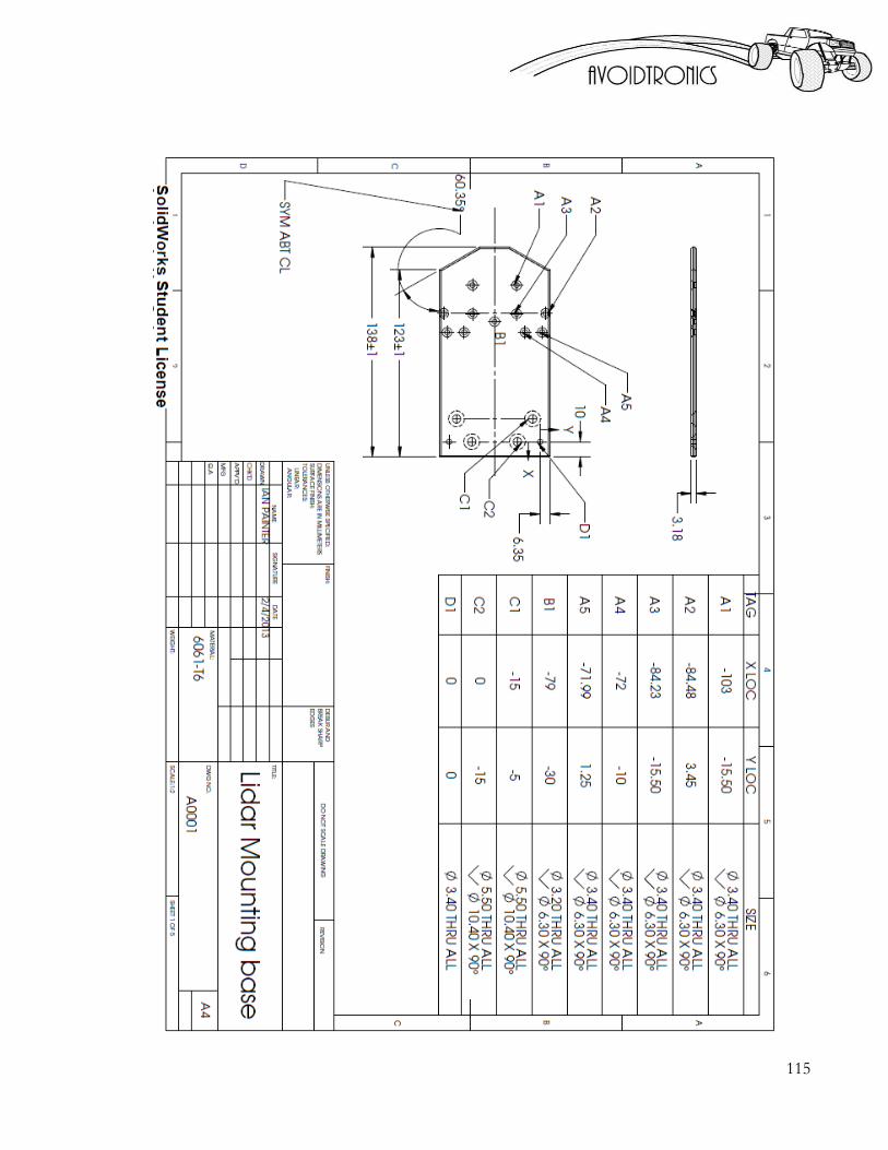
115

116
Appendix P Li-Ion Cell Specification Sheet