autonomous guided vehiclesummitraj.tripod.com/agv/final.pdfthe autonomous guided vehicle (agv)...
TRANSCRIPT
AUTONOMOUS GUIDED VEHICLE
By
EE32042 SUMMIT RAJ TULADHAR EE32040 DIPESH GHIMIRE EE32014 SHAILENDRA JOSHI EE32038 ABHINAYA JOSHI ME32065 PRAVEEN KUMAR YADAV ME32055 KISHOR JOSHI CE32108 BINSAN KHADKA CE32103 DIGDARSHAN LAL DHONJU CE32104 SHREE KRISHNA SHRESTHA CE32116 YANZEEV MAHARJAN CE32118 MANOZ CHANDI SHRESTHA
School of Engineering KATHMANDU UNIVERSITY
June, 2002

i
CERTIFICATE
AUTONOMOUS GUIDED VEHICLE
School of Engineering KATHMANDU UNIVERSITY
June, 2002 Approved by: Supervisor(s) ____________________________ ____________________________ ____________________________ ____________________________ Head of Department ______________________ Date ___________
ii
ABSTRACT The Autonomous Guided Vehicle (AGV) Project aspires to construct a vehicle automatically guided without wires and with some intelligence to choose the correct path of travel. The AGV has two front wheels driven by two PMDC motors and a free castor wheels at the back. For the simplest automation, the AGV would be following a line on a floor, either by image processing or by IR-Emitter-Detector sensors. The image is captures by a CCD Camera and sent to the frame grabber of the onboard computer. The computer processes the image and sends information to the motor drive circuits. Speed control of the motors is done by driving an H-Bridge with Pulse Width Modulated signal. The AGV robot can be remotely controlled, using AM transmitter receiver operating at 418 MHz. The working range is about 70 meters. The AGV Vehicle also has two pairs of 40 KHz ultrasonic transmitter/receiver at the front. On sensing an obstacle on the vehicle's direction of movement, the AGV stops, steers and tries again. Thus, the AGV is a good platform for robotics. On availability of good sensors, the AGV project can be extended to make a more sophisticated robot in the future.

iii
ACKNOWLEDGEMENT
At the outset we are thankful to God Almighty for his unending grace and sustenance which carried us through our endeavour. We heartily acknowledge Er. Projjwol Dhakal, Er. Sandip Kumar Suman, Er. Ranjan Sitaula from the Department of Mechanical Engineering, Er. Mahesh Raman Neupane, Er. Janak Shrestha, Er. Rajendra Aryal, Er. Rabindra Ghimire, Er. Naresh Yadav from the department of Electrical and Electronics Engineering, and Er. Saurabh Dass Manandhar, and Er. Bibek Agrawal from the Department of Computer Engineering for expressing their confidence in us by giving such a challenging project. Words would be insufficient to express our heart-felt gratitude to the department faculties for rendering their unflinching support and guidance throughout the duration of our project work. We also thank the faculties of the E&E, CE, and ME Departments who were directly or indirectly involved with our project. Last but not the least; we would like to thank our fellow college-mates and some junior and senior students, especially Mr. Prakash Manandhar, for their kind and highly valuable advices.

iv
TABLE OF CONTENTS Contents Page No. 1. Introduction................................................................................................................1
1.1. The Project and its Aims......................................................................................1 1.2. The Team and the Plan followed .........................................................................1 1.3. Report Overview..................................................................................................2
2. Robotics .....................................................................................................................3 2.1. Introduction..........................................................................................................3 2.2. The R&D in Robotics ..........................................................................................4 2.3. AGV Products......................................................................................................5 2.4. AGV as a Robot ...................................................................................................5
3. Mechanical Design.....................................................................................................6 3.1. Introduction..........................................................................................................6 3.2. Brief Description of the Mechanical Components ..............................................6
3.2.1. Wheels and Tyres..........................................................................................6 3.2.2. BEARINGS ...................................................................................................9 3.2.3. SHAFTS ......................................................................................................10 3.2.4. FRAME.......................................................................................................12 3.2.5. Sprocket.......................................................................................................12 3.2.6. Chain ...........................................................................................................12 3.2.7. Castor wheel................................................................................................13
3.3. Design Criteria ...................................................................................................13 3.4. Design Options ..................................................................................................14
3.4.1. MODEL 1....................................................................................................14 3.4.2. MODEL 2....................................................................................................14 3.4.3. Model Selection...........................................................................................14
3.5. Brief of the manufacturing processes during fabrication ..................................15 3.6. DESIGN CALCULATIONS.............................................................................17
3.6.1. Calculation of Power of Motor....................................................................17 3.7. Shaft Design.......................................................................................................19 3.8. Bearing Selection...............................................................................................22 3.9. Problems raised during fabrication and remedies..............................................23 3.10. Final Design Values of the Vehicle:................................................................24 3.11. Outside Diameter : 43 cm................................................................................24 3.12. COST ESTIMATION......................................................................................26
4. Software Design.......................................................................................................27 4.1. Introduction........................................................................................................27 4.2. Image Processing Approach ..............................................................................27 4.3. Digital Image Processing ...................................................................................28 4.4. Image Acquisition..............................................................................................29
4.4.1. Preliminaries................................................................................................29 4.4.2. Camera components ....................................................................................31 4.4.3. Camera solution to obtain intensity images ................................................32

v
4.5. Camera parameters and calibration ...................................................................35 4.5.1. Basic Optics.................................................................................................35 4.5.2. Image Focusing ...........................................................................................36
4.6. Geometric Image Formation..............................................................................37 4.7. Camera Parameters ............................................................................................40 4.8. Intrinsic Parameters ...........................................................................................42 4.9. Camera Models Revisited ..................................................................................44 4.10. Noise Theory ...................................................................................................49
4.10.1. Image Noise...............................................................................................49 4.10.2. Noise Amount ...........................................................................................49 4.10.3. Gaussian Noise ..........................................................................................50 4.10.4. Impulsive Noise.........................................................................................50
4.11. Block diagram of image processing model .....................................................51 4.12. Image Analysis ................................................................................................51 4.13. Edge Detection.................................................................................................52
4.13.1. Gradients Operators...................................................................................54 4.13.2. Compass operators ....................................................................................55
4.14. The Hough Transform .....................................................................................56 4.14.1. Working Principle of Hough Transform...................................................56
4.15. Platform Used: Microsoft Visual C++.............................................................61 4.16. Image Processing Libraries..............................................................................62
4.16.1. Intel OpenCV ............................................................................................62 4.16.2. Microsoft Vision SDK ..............................................................................62
4.17. The Parallel Port ..............................................................................................63 4.17.1. Unidirectional (4-bits)...............................................................................64 4.17.2. Bi-directional (8-bits) ................................................................................64 4.17.3. Enhanced parallel port (EPP) ....................................................................65 4.17.4. Enhanced capability port (ECP) ................................................................65
4.18. Functions and Properties of Classes ................................................................66 4.18.1. CAgv .........................................................................................................67 4.18.2. CVision......................................................................................................68 4.18.3. CProcess ....................................................................................................70 4.18.4. CDecision..................................................................................................71 4.18.5. CInterface..................................................................................................72
4.19. Wireless Control Approach .............................................................................73 4.19.1. MSComm Control.....................................................................................73 4.19.2. Serial Port ..................................................................................................75 4.19.3. Serial Port Configuration: .........................................................................76 4.19.4. USER INTERFACE..................................................................................77
5. Electronic Design.....................................................................................................78 5.1. Introduction........................................................................................................78
5.1.1. CCD Camera – Image Processing Mode.....................................................78 5.1.2. Ultrasonic Mode – Obstacle Avoidance......................................................79 5.1.3. Emitter Detector – Line Following .............................................................79 5.1.4. Manual Wireless Control Mode ..................................................................79
5.2. DC Motor ...........................................................................................................79

vi
5.2.1. Construction of the DC Motor ....................................................................80 5.2.2. PMDC Motors.............................................................................................80 5.2.3. Characteristics of DC motor........................................................................81 5.2.4. DC Motor Used ...........................................................................................82
5.3. Speed Control of DC Motor ..............................................................................83 5.3.1. Chopper and PWM......................................................................................83
5.4. H-Bridge ............................................................................................................87 5.4.1. Theory .........................................................................................................87 5.4.2. H-Bridge Design .........................................................................................90
5.5. Software – Hardware Interface ..........................................................................92 5.5.1. Introduction.................................................................................................92 5.5.2. Multiplexing ................................................................................................93 5.5.3. PWM Generation.........................................................................................95 5.5.4. Direction Control.........................................................................................95 5.5.5. Fault Tolerance System...............................................................................96
5.6. The Basic Stamp II ............................................................................................97 5.6.1. Introduction.................................................................................................97 5.6.2. Program.......................................................................................................99
5.7. Image Processing Mode...................................................................................108 5.8. Ultrasonic Mode ..............................................................................................108
5.8.1. Ultrasonic Tone Generation......................................................................109 5.8.2. Signal Conditioning...................................................................................109
5.9. Emitter Detector Mode ....................................................................................110 5.10. Wireless Control Mode ..................................................................................111
5.10.1. Level Shifting ..........................................................................................112 5.10.2. AM Transmission and Reception............................................................112
5.11. Power Supply.................................................................................................112 6. The Product............................................................................................................114
6.1. Introduction......................................................................................................114 6.2. Gantt chart .......................................................................................................115 6.3. Conclusion and Recommendation...................................................................116
7. Bibliography...........................................................................................................117 8. Appendix................................................................................................................119
8.1. Mechanical Drawings:.....................................................................................119 8.2. Image Processing Code in VC++ using VisionSDK .......................................122 8.3. Wireless Serial Communication for Remote Control Code in VB..................139

vii
LIST OF FIGURES S.No. Title Page
Fig 2. Shaft Design.....................................................................................................19 Fig 3. Image Processing Approach Outline................................................................27 Fig 4. Digital Image Processing Sequence Block Diagram.......................................28 Fig 5. Basic CCD Theory...........................................................................................30 Fig 6. How the three colors mix to form many colors ...............................................33 Fig 7. How the original image at the left is split in a beam splitter. .........................33 Fig 8. A spinning disk filter. ......................................................................................34 Fig 9. The basic element of an Imaging System ........................................................36 Fig 10. The Perspective Camera Model. ..................................................................37 Fig 11. The Relation between camera and world coordinate frames .......................41 Fig 12. Block Diagram of Software model (Image Processing Approach) .............51 Fig 13. Edge detection via gradient operator ...........................................................54 Fig 14. Edge detection via compass operator...........................................................55 Fig 15. Coordinate points and possible straight line fittings ....................................57 Fig 16. Parametric description of a straight line. .....................................................57 Fig 17. Original and Edge Detected Image ..............................................................59 Fig 18. The Hough Transformed Image ...................................................................60 Fig 19. The Parallel Port Connector .........................................................................63 Fig 20. Relationship between classes.......................................................................66 Fig 21. Wireless Control Approach Block Diagram................................................73 Fig 22. 9-pin AT Serial Port Connector ...................................................................76 Fig 23. 25-pin Serial Port Connector .......................................................................76 Fig 24. Characteristics of Shunt DC Motors (V, If constant) ..................................81 Fig 25. The DC Motor used for the AGV ................................................................82 Fig 26. An Elementary Chopper Circuit and (b) output voltage and current
waveforms .............................................................................................................84 Fig 27. Principle of Pulse Width Modulation (Constant T) .....................................85 Fig 28. Principle of Frequency Modulation (a) on-time Ton constant and (b) off-
time Toff constant .................................................................................................86 Fig 29. BJT H-Bridge ...............................................................................................87 Fig 30. The H-Bridge with left to right current flow ...............................................88 Fig 31. The H-Bridge with Enable Circuitry............................................................89 Fig 32. Power H-Bridge Design ...............................................................................90 Fig 33. Power Derating of the 2N3055/MJ2955 transistors.....................................91 Fig 34. Multiplexing.................................................................................................94 Fig 35. PWM Generator ...........................................................................................95 Fig 36. Direction Control .........................................................................................95 Fig 37. A Flag setting/resetting mechanism.............................................................96 Fig 38. The Basic Stamp II IC..................................................................................97 Fig 39. The Ultrasonic Transmitter Receiver Pair Arrangement ...........................109 Fig 40. Ultrasonic Receiver Signal Conditioning ..................................................109 Fig 41. Emitter Detector Sets. ................................................................................110

viii
Fig 42. Infrared Emitter Detector Arrangement .....................................................111 Fig 43. RS-232C to Inverted TTL Level Shifter....................................................112 Fig 44. Caster Wheel..............................................................................................119 Fig 45. Caster Angle...............................................................................................119 Fig 46. FINAL DESIGN OF THE VEHICLE.......................................................120 Fig 47. TOP VIEW OF THE VEHICLE................................................................120 Fig 48. FRONT VIEW OF THE VEHICLE ..........................................................121 Fig 49. LEFT VIEW OF THE VEHICLE.............................................................121

ix
LIST OF TABLES
S.No. Title..........................................................................................................Page Table 1. Standard Parallel Port pin-out ......................................................................63 Table 2. Important MSComm Control Properties......................................................74 Table 3. 9-pin Serial Port Pin-Out .............................................................................76 Table 4. 25-pin Serial Port Pin-Out ...........................................................................76 Table 5. Standard Serial I/O Port Addresses and Interrupts ......................................77 Table 6. 2N3055/MJ2955 Transistor Ratings ............................................................91 Table 7. On Characteristics of the 2N3055/MJ2955 transistors ................................92 Table 8. Basic Stamp II Pin Configuration................................................................98 Table 9. Basic Stamp II Pin Assignments ..................................................................99 Table 10. Mode Selection ......................................................................................100 Table 11. Parallel Port Pin Assignments................................................................108

1. .
1. Introduction
1.1. The Project and its Aims
The project aims at building a programmable robot. By the term robot, a small
dynamic vehicle is to be understood. Once the robot has been programmed, it
should have an autonomous control over its job, guided by some means.
This Autonomous Guided Vehicle (AGV) is a mechanical challenge to design
and construct a suitably sized vehicle, with a maximum specified weight (its own
and the payload it could carry) able to tread on any given terrain.
AGV stands as an electronic challenge so as to design a control system in
between the mechanical drive and the output control signals from the onboard
computer, a reliable on board power supply system, and proper feedback system
to dead reckon for good navigation.
Bringing life to the AGV is a software challenge. The sole purpose of the life of
the AGV should be programmable, and could be changed as per requirement.
This project specifies the aim of the AGV to be a line follower.
1.2. The Team and the Plan followed
This project is a part of the third year Engineering course offered at Kathmandu
University, School of Engineering. The project team consists of third year
engineering students from the Mechanical (ME), Electrical & Electronics (EE),
and the Computer Engineering (CE) faculties.
The initiation of the project work started with the formation of the project team
on Mid-August 2001. The Project was completed on June 2002. On the first half
of the project, the team spent most of the time gathering resources, and building
ideas with necessary laboratory work. On the other half of the project, the ideas
were implemented to finally engineer a working vehicle. Details of the work
done can be found on Section 6.2

2. .
1.3. Report Overview
This report is divided into three main parts - Mechanical Design, Electronic
Design, and Software Design. The report is further divided into eight chapters,
the first being this introduction. The second chapter will briefly deal about
robotics and the research being done worldwide. The third, fourth and fifth
chapters will include the three aspects of engineering involved in the design and
construction of the AGV - Mechanical, Electrical, and Software respectively.
The Sixth chapter is about the final product and the progress done by the team.
The final seventh and eighth chapters are the references and the appendix. A
Block diagram of the AGV Design, with an input of the image from the camera,
and an output of the control of motor is shown in Figure 1.
Fig 1. Block Diagram of AGV

3. .
2. Robotics
2.1. Introduction
Robotics is the leading field in Science & Technology which is going to shape
the future of the human race. Since robots are used mainly in manufacturing, we
see their impact in the products we use every day. Usually this results in a
cheaper product. Robots are also used in cases where it can do a better job than a
human such as surgery where high precision is a benefit. And, robots are used in
exploration in dangerous places such as in volcanoes which allows us to learn
without endangering ourselves.
The word "robot' was coined by Karel Capek who wrote a play entitled "R.U.R."
or "Rossum's Universal Robots" back in 1921. The base for this word comes
from the Czech word 'robotnik' which means 'worker'. In his play, machines
modeled after humans had great power but without common human failings. In
the end these machines were used for war and eventually turned against their
human creators.
Popular science fiction writer Isaac Asimov created the Three Laws of Robotics:
#1 A robot must not injure a human being or, through inaction, allow a human
being to come to harm.
#2 A robot must always obey orders given to it by a human being, except where
it would conflict with the first law.
#3 A robot must protect it's own existence, except where it would conflict with
the first or second law.
The population of robots is growing rapidly. This growth is lead by Japan that
has almost twice as many robots as the USA. All estimates suggest that robots
will play an ever- increasing role in modern society. They will continue to be
4. .
used in tasks where danger, repetition, cost, and precision prevents humans from
performing.
2.2. The R&D in Robotics
We live in a truly amazing, high technology world. The state of the art has a host
of known problems with known solutions. The World Wide Web is making a
tremendous amount of information available to everyone. The making of an
intelligent robot is the ideal vision for all robotic enthusiasts. All one has to do to
see the intelligent robot model is to look in a mirror. Ideally, all intelligent robots
move dexterously, smoothly, precisely, using multiple degrees of coordinated
motion and do something like a human but that a human now doesn’t have to do.
They have sensors that permit them to adapt to environmental changes.
They learn from the environment or from humans without making mistakes.
They mimic expert human responses. They perform automatically, tirelessly, and
accurately. They can diagnose their own problems and repair themselves. They
can reproduce, not biologically but by robots making robots. They can be used in
industry for a variety of applications. A good intelligent robot solution to an
important problem can start an industry and spin off a totally new technology.
For example, imagine a robot that can fill your car with gas, mow your lawn, a
car that can drive you to work in heavy traffic, a machine that repairs itself when
it breaks down, a physician assistant for microsurgery that reconnects 40,000
axons from a severed nerve.
Intelligent robots are also a reality. Many are used today. Many more prototypes
have been built. Typical applications are: high speed spot welding robots, precise
seam welding robots, spray painting robots moving around the contours of an
automobile body, robots palletizing variable size parcels, robots loading and
unloading machines.

5. .
2.3. AGV Products
AGV has found different levels of applications around the world. They are used
in factories, hospitals carrying things around. They have also found a good use
around the house as Autonomous Vacuum Cleaners.
2.4. AGV as a Robot
AGV has been a dream. An autonomous robot is a dream for now, a vehicle
doing jobs for you, like bringing you a cup of coffee in the morning from the
coffee maker in the kitchen. To make this dream a reality, we have to start from
collecting the stones to build it. Collecting stones and making a skeletal robot is
our aim for this project, which should have elementary vision capability, like line
following.

6. .
3. Mechanical Design
3.1. Introduction
The AGV has stood as a mechanical challenge from the very first stages of the
project. The mechanical design would determine directly or indirectly the rest of
the design processes - electrical, electronics, and software.
The AGV design should minimize weight to reduce power required, as high
power drives are not easily available and portable. The basic design requirements
for the AGV are steering and forward and reverse drive. The drive could be
either electrical or fuel. The fuel engine alternative is not feasible under the
presumed vehicle dimension and weight. An electrical drive system is more
viable for the AGV as visualized by the team.
3.2. Brief Description of the Mechanical Components
3.2.1. Wheels and Tyres
The importance of wheels and tyres in the automobile is obvious. Wheels are the
important parts of the vehicle as they must support the weight of the vehicle and
help protect it from the road shocks. In addition, the rear wheels must transmit
the power, the front wheels must steer the vehicle, and all must resist braking
stresses and withstand side thrusts. Wheels must be perfectly balanced.
The various requirements of an automobile wheel are:
i) It should be balanced both statically and dynamically.
ii) It should be lightest possible so that the up sprung weight is least.
iii) Its material should not deteriorate with weathering and age.
Types of wheels
There are three types of wheels, viz the pressed steel disc wheel, the wire wheel,
and the light alloy cast wheel.

7. .
Because of simplicity, robust construction, lower cost of manufacture and ease in
cleaning, the steel disc wheel is used universally. The disc wheel consists of two
parts, a steel rim which is well based to receive the tyre and a pressed steel disc.
The rim and the disc may be integral, permanently attached, depending upon the
design.
The wire wheel has a separate hub, which is attached to the rim through a
number of wire spokes. The spokes carry the weight, transmit the driving and
braking torques and withstand the side forces. Spokes are long, thin wires and as
such these cannot take any compressive of bending stresses.
Cast wheels are generally used in cars while forged wheels are preferred for
heavy vehicles. The main advantage of light alloy wheels is their reduced weight
which reduces unsprung weight.
TYRES
A tyre is a cushion provided with an automobile wheel. It consists of mainly the
outer cover i.e., the tyre proper and the tube inside. The tyre tube assembly is
mounted over the wheel rim. It is the air inside the tube that carries the entire
load and provides the cushion.
The tyre performs the following functions;
o To support the vehicle load
o To provide cushion against shocks
o To transmit driving and braking forces to the road.
o To provide cornering power for smooth steering.
Types of Tyres
The different types of tyres are
a) Pneumatic tyre

8. .
b) Tube tyre
c) Tubeless tyre
The pneumatic tyres are designed to cushion the vehicle and its load from the
shocks and vibrations resulting from road inequalities. The use of solid tyres on
automobiles is now obsolete and only the pneumatic tyres are used universally.
These pneumatic tyres are of two types, the conventional tyre with a tube and the
tubeless tyre. The conventional tube tyre consists of two main parts, viz. The
carcass and the tread. The carcass is the basic structure taking mainly the various
loads and consists of a number of plies wound in a particular fashion. The tread
is the part of the tyre which contacts the road surface when the wheel rolls. It is
generally made of synthetic rubber.
Inside the tyre, there is a tube which contains the air under pressure. The tube
being very thin and flexible, takes up the shape of the tyrecover when inflated. A
valve stem is attached to the tube for inflating or deflating the same.
Desirable tyre properties:
Non-skidding
This is one of the most important tyre properties. The tread pattern on the trye
must be suitably designed to permit least amount of skidding even on wet road.
Uniform Wear
To maintain the non skidding property, it is very essential that the wear on the
tyre tread must be uniform. The ribbed tread patterns help to achieve this.
Load Carrying
The tyre is subjected to alternating stresses during each revolution of the wheeel.
The tyre material and design must be able to ensure that the tyre is able to sustain
these stresses.

9. .
Cushioning
The tyre should be able to absorb small, high frequency vibrations set up by the
road surface and thus provide cushioning effect.
Power Consumption
The automotive tyre does absorb some power which is due to friction between
the tread rubber and the road surface and also due to hysterisis loss on account of
the tyre being continuously flexed and released. This power comes from the
engine fuel and should be the least possible. It is seen that the synthetic tyres
comsume more power while rolling than the ones made out of natural rubber.
Tyre Noise
The tyre nose may be in the form of definite pattern sing, a sequel or a lous roar.
In all these cases, it is desirable that the noise hould be minimum
Balancing
This is very important consideration. The tyre being a rotating part of the
automobile, it must be balanced statically as well as dynamically. The absence of
balancing gives rise to peculiar oscillations
3.2.2. BEARINGS
Bearing is a machine element, which supports another machine element or
member permitting the relative motion between the contact surfaces. There are
two types of bearings - Sliding contact bearing or Journal bearing and Rolling or
Anti friction bearing.
Types of Bearings:
Rolling or Anti friction bearing
The term rolling contact bearing, anti friction bearing and rolling bearings are all
used to describe that class of bearing in which the main load is transferred

10. .
through element in rolling contact rather than in sliding contact. In a rolling
bearing, the starting friction is twice the running friction but still it is negligible
in comparison to the starting friction of journal bearing.
Types of rolling contact bearings
-Ball bearings
-Roller bearings
Ball bearings:-
A ball bearing consists of following parts- outer race ,inner race, balls, and
retainer. The outer and inner races are held concentric with each other by several
spherical balls placed circumferentially equal. The ball retaining rings,(usually in
two parts) ensure the equal spacing of the balls. the grooves, which form the path
for the rolling elements, are known as raceways. Depending on the type of the
load the bearing has to support, it may be either designed for radial load or axial
load or both for combined. When a ball bearing supports only a radial load, the
plate of the rotation of the ball is normal to the center line of the bearing. In the
case of the axial loading, the axial shifts the plane of rotation of the balls.
3.2.3. SHAFTS
A shaft is a rotating member, usually of circular cross-section (either solid or
hollow), transmitting power. It is supported by bearings, wheels etc. and is
subjected to torsion and to transverse or axial load, acting singly or in
combination. Generally shafts are not of uniform diameter but are stepped to
provide shoulders for locating gears, pulleys, bearings etc. An axle is a stationary
member primarily loaded in bending with rotating wheels, pulleys, etc. Short
axles and shafts are often called spindles. Regardless of design requirement, care
must be taken to reduce the stress concentration in notches, keyways, etc.

11. .
Power consideration of notch sensitivity may improve the strength more
significantly than material consideration.
Material used for shaft
Generally shafts are made up of mild steel in ordinary case. When strength is
required alloy steel such as nickel, nickel-chromium or chrome vanadium steel is
used.
Types of shaft
-Transmission shaft
-Machine shaft
Transmission shaft
These shafts transmit power between the source and the machines absorbing
power. The counter shaft, line shafts, overhead shafts and all factory shafts are all
transmission shafts. Since these shafts carry machine parts such as pulleys, gears,
etc, therefore they are subjected to bending in addition to twisting.
Machine shaft.
These shaft form an integral part of machine itself. The crankshaft is an example
of machine shaft.
Stresses in Shaft
The following stresses are induced in the shafts
Shear stresses due to transmission of torque.
Bending stresses due to forces acting upon the machine elements like gears,
pulleys, etc. as well as due to the weight of the shaft itself.
Stresses due to combined torsion and bearing loads.

12. .
3.2.4. FRAME
Frame is made up of Galvanized iron pipe and sheet. The functions of frame are
as follows
A. To support the components, motor, camera, CPU etc.
B. To withstand static and dynamic load wit deflection or distortion.
Loads on the frame
a. Vertical loads when the wheel chair come across a bump or hump (which
results in longitudinal torsion in longitudinal torsion due to one wheel lifted or
lowered and other wheel at the usual road level .
b. Loads due it road chamber side wind, concerning force while taking a turn(
which results I lateral bending of side members).
c. Load due to wheel impact with road obstacles i.e., one wheel tends to move (
which cause distorting the frame to parallelogram shape).
d. Motor torque and braking torque (which cause to bend the side member in
vertical plane).
e. Sudden impact load during collision 9which may result in a general collapse).
3.2.5. Sprocket
Two sprocket of same size and same no. of teeth will be used to transmit power
of motor to shaft of wheel at the same rpm.
3.2.6. Chain
A chain is a mechanical component which will be fitted over the teeth of the
sprocket for the transmission of the power from the motor to the shaft of the
wheel.

13. .
3.2.7. Castor wheel
The angle between the king pin centre line and the vertical, in the plane of the
wheel is called the castor angle. If the king pin centre line meets the ground at a
point in front of the wheel centre line, it is called positive castor while it is
behind the wheel centre line, it is called negative castor.
Positive castor on the car wheels provides directional stability. The positive
castor causes the wheel to be pulled in any direction.
Castor has another effect also. When the vehicle having positive castor takes a
turn, the outer side of the vehicle is lowered while the inner one is raised, i.e. the
positive castor help the centrifugal force in rolling out the vehicle.
3.3. Design Criteria
The final goal of the mechanical design is to fabricate a vehicle that is safe,
economical and that is practical to manufacture. Different design approaches
must have to be adjusted to be compatible with the market. In approaching the
final design some criteria should be established to guide decision making
processes. The following are the design criteria that should be established in
designing the project.
The design of the vehicle and its various components for efficient operation.
o Selection of proper material
o Safety of operation
o Economic status

14. .
3.4. Design Options
3.4.1. MODEL 1
The vehicle can be made of four wheels. In this type of vehicle power is given to
the shaft by means of motor and the differential gear is used in rear wheel for the
turning of the wheels and another motor is connected with the steering which is
used for turning front wheels.
3.4.2. MODEL 2
This model consist of three wheels. Two of them as rear wheel and one as front
wheel. The two rear wheels would be driven by the DC motors. In this type of
vehicle , motor is connected to the shaft of each wheels by means of chain and
sprocket which is responsible for transmission of power. The ball castor is placed
as the front wheel which can rotate in any direction to provide more degree of
freedom to the vehicle.
3.4.3. Model Selection
Since the differential gear costs about eight thousand rupees, it will be difficult
for us to install it from economical point of view. Also the steering system to be
used for the turning movement of the vehicle will make difficult for the design of
the vehicle. In the second model, the vehicle can be turned by varying the speed
of the two motors, which are connected separately to two wheels. Also, the ball
castor assembly as the front wheel will make easier for the turning movement of
the wheel. Since it is also appropriate from cost point of view, we select model
second for the design of the vehicle.
Working Principle of the selected Model:
The model we choose mainly consists of two 45 cm bicycle tyre, bearings,
frames, shafts, chains, sprockets, ball castor as the mechanical part. Two 45 cm
bicycle tyres are used as the rear wheels. Two electrical dc motors are connected

15. .
to the two wheels separately. The speed of the two motors controls the movement
of the vehicle. By varying the speed of the motors, the turning movement of the
vehicle can be obtained. The shaft of wheel and motor is connected with chain
and sprocket. sprocket of same size will be fitted on the shaft of wheel and motor
so that same rpm is transmitted to wheel from motor.
For the placement of the other electrical and computer parts ,a frame made up of
iron rod and plywood is placed as the base Firstly, the iron rod is fixed in
position by the process of welding and upon which plywood are fixed by the
process of drilling.
Two individual shafts are placed for the transmission of the power from the
motor to the wheel. On each shaft and on the motor, sprocket is fixed and chains
are placed over it for the transmission of the power. The fabrication of the
vehicle is done in such a way that most of the parts can be disassembled easily i.e
welding process is avoided as far as possible
To prevent damage to the electrical and computer parts, the vehicle incorporates
the covering.
3.5. Brief of the manufacturing processes during fabrication
There are different manufacturing processes that were to be gone through in
order to complete the fabrication of the vehicle. All the operations are performed
in the workshop. The operations performed are
1) Welding
2) Drilling
3) Cutting
4) Grinding
5) Facing

16. .
6) Turning
7) Thread Cutting
Welding operation was performed to join the different components of the
vehicle. The base of the vehicle is made of mild steel. The mild steel of size
73cm × 51 cm was joined for the base of the vehicle. Similarly, other
components like the castor wheel was welded on the base of the vehicle. Welding
operation was also carried to fix the motor-stand.
Drilling operation was performed to place the bearing cap on the frame of the
vehicle. In the same way, drilling was also performed to assemble the castor
wheel to the vehicle.
Cutting operations were performed to obtain the required sizes of the base of the
vehicle. Hand grinding operation was performed to make the welded surfaces
smooth.
Facing and the turning operations were carried out in lathe to make the shaft for
the vehicle. Threads were also made in the shaft with the help of thread cutting
die. The specifications of the die is
Tap size: ¾” Tap Size : ½”
Drill Size : 16.25 mm Drill size : 10.5 mm

17. .
3.6. DESIGN CALCULATIONS
3.6.1. Calculation of Power of Motor
Diameter of wheel, D = 43cm = 0.43m
Radius of wheel, R = 21.5cm = 0.215m
Circumference = 2πR
= 2* π* 0.215 = 1.35m
Required Speed of the wheel = 1m/s = v
Angular velocity (ω) = 2πn / 60
therefore,
v = r ω
or, v = r 2πn/60
or, n= 60 *v /2πr
= 60 * 1/ (2π *0.215)
= 44.41rev/min
thus, required rpm of motor = 44.41 rpm
Now, Angular Velocity(ω) = 2πn / 60
= 2π * 44.41/ 60
= 4.64 rad/sec
Self weight of the vehicle = 10 kg
Weight on the body = 15 kg

18. .
Net weight (ω) = 25kg = 245 N
Let us consider,
Maximum Frictional force =Fs
Coefficient of static friction = µs =0.4
Now, µs = Fs /W
therefore, Fs = µs * W
= 0.4 * 245 N
= 98 N
therefore, Initial torque = Fs * R
= 98 * 0.25
= 21.07 N-m
This torque is the maximum torque that is required. But during the motion the
frictional forces reduces because of the lower value of coefficient of friction.
Frictional force in motion = Fd
Coefficient of dynamic friction = µd = 0.25
Now, µd = Fd /W
therefore, F d = µd * W
= 0.25 * 245
=61.25
Torque (τ) = F d * R
= 61.25 * 0.215 = 13.16 N-m, which is required running Torque.
Power required by the motor = τ * 2πn/ 60
= 13.16 * 2 * 3.14 * 44.41 / 60
= 61.2 watt
= 0.082 hp.
Therefore, the required motor Power = 0.082 hp.
19. .
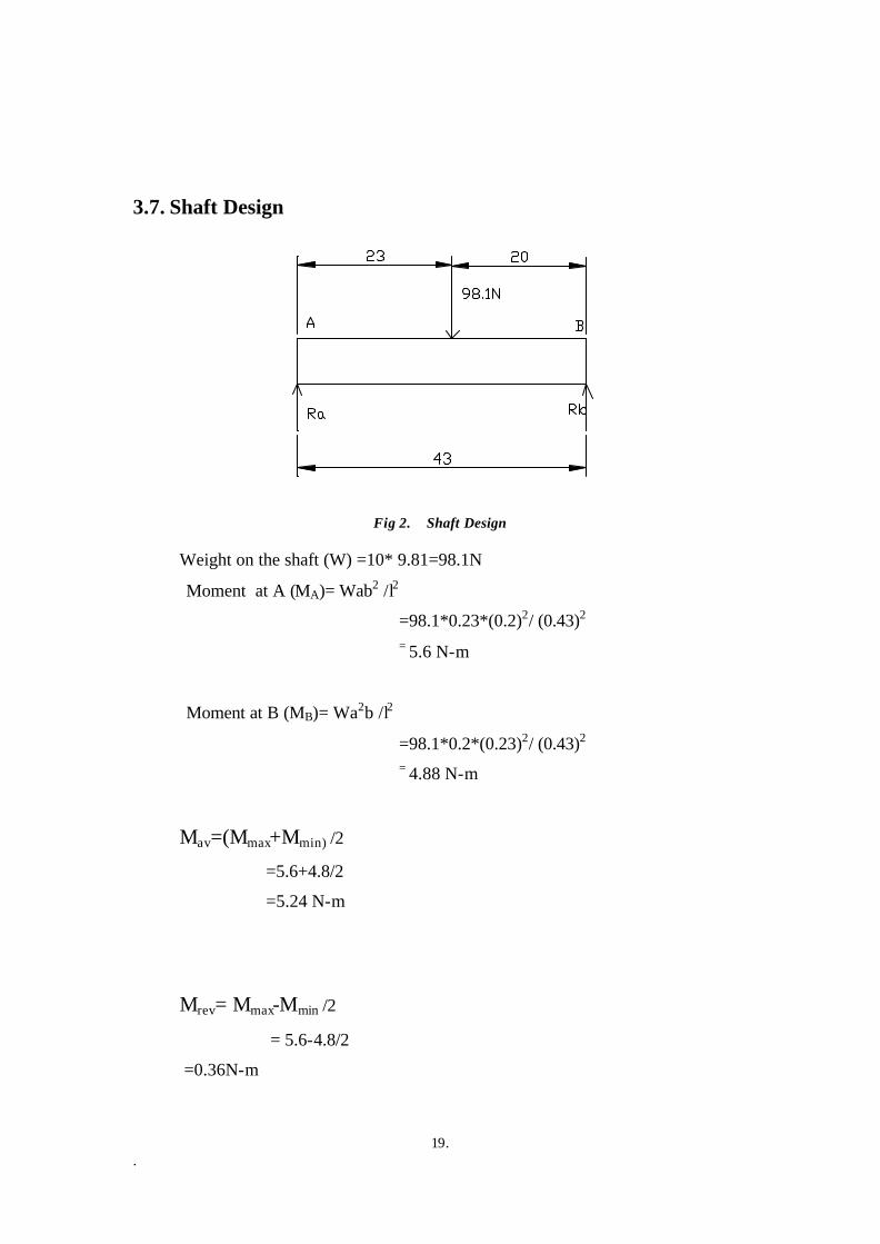
3.7. Shaft Design
Fig 2. Shaft Design
Weight on the shaft (W) =10* 9.81=98.1N
Moment at A (MA)= Wab2 /l2 =98.1*0.23*(0.2)2/ (0.43)2
= 5.6 N-m
Moment at B (MB)= Wa2b /l2
=98.1*0.2*(0.23)2/ (0.43)2
= 4.88 N-m
Mav=(Mmax+Mmin) /2
=5.6+4.8/2
=5.24 N-m
Mrev= Mmax-Mmin /2
= 5.6-4.8/2
=0.36N-m

20. .
A shaft subjected to transmit torque with gear, pulley, sprocket or similar devices
result in bending moment as well as torque acting on the shaft and the relationship of
combined stresses to fatigue failures must be considered. For this maximum shear
stress theory is used for the ductile material.
ëmax=[(ó/2)2+ ë2 ]1/2
For bending only
Fos=óy/ óav+Kf ór(óy/óe)
= óy/ ómax
For shear stress part,
Fos=ëy/ [ëav+(Kf)s ër(ëy/ ëe)]
= ëy /ë max
For combined bending and torsion,
Fos= ëy /[1/4{ 2 Mav/J *d/2+ Kf 2 Mrev/J*d/2 * óy/óe}2 +{ Tav /J *d/2
+Kfs *Tr/J *d/2* ëy/ ëe}2 ]1/2
Where, J=ð d4/32 =polar moment of inertia
.d3 =Fos*16 [1/4{ 2 Mav/J *d/2+ Kf 2 Mrev/J*d/2 * óy/óe}2 +{ Tav /J *d/2
+Kfs *Tr/J *d/2* ëy/ ëe}2 ]1/2 /ð ëy
Tmax=21.07 N-m
Tmin=13.16 N-m

21. .
Hence,
Tav= Tmax + Tmin /2
= (21.07+13.16)/2
= 17.11 N-m
Trev = Tmax - Tmin /2
=(21.07-13.16)/2
= 3.95 N-m
For mild steel,
óy =304.11* 106 N/mm2
[DESIGN DATA,PSG COLLEGE OF TECHNOLOGY
óe =568.98* 106 N/mm2 PAGE 1.9 ]
[
ëy = óy /2 =152.05 *106 N/mm2
ëe = óe/2 =284.49* 106 N/mm2
Therefore,
d3 = 2 *16 *[(30.56 +411.14)]1/2 /ð *152.05 *106
d=.0112m
d=11.2mm =12mm
Hence, the diameter of the shaft = 12mm

22. .
3.8. Bearing Selection
Diameter of the shaft = 16mm
From, DESIGN DATA, PSG COLLEGE OF TECHNOLOGY,
Page 4.14
Bearing of basic design no.(SKF) =6201
ISI No. =15BC02
Outer diameter = 42mm
Inner diameter =16mm
Dynamic load rating capacity (c) =610 Kgf
Maximum permissible speed (rpm)=16000
For shaft diameter = 20mm
From, DESIGN DATA, PSG COLLEGE OF TECHNOLOGY,
Page 4.14
Bearing of basic design no.(SKF) =6304
ISI No. =20BC03
Outer diameter = 52mm
Inner diameter =20mm
Dynamic load rating capacity (c) =1250 Kgf
Maximum permissible speed (rpm)=13000

23. .
3.9. Problems raised during fabrication and remedies
1) Wheel Drive:
During the design of the vehicle, the vehicle was made four wheeler with two bicycle
tyres as the front wheel and two wheels as the rear wheel. But, while taking a turn,
there is probability of skidding off the vehicle. So instead of the tyres, ,two ball
castors is used as the rear wheel. Again during the fabrication of the vehicle, the
vehicle is made three wheeler with the ball castor as the front wheel and the two tyres
as the rear wheel as it provides more degree of freedom to the vehicle.
2) Shaft:
Generally in the vehicle, power is supplied to single shaft for the driving mechanism
and the differential gear is provided for the turning movement of the vehicle. As the
differential gear is expensive one, different option was to be considered. So,
individual power is given to two wheels by the use of chain and sprocket through two
motors. It also enables to change the direction of the vehicle by varying the power of
the two motors.

24. .
3.10. Final Design Values of the Vehicle:
Following parameters and specifications are designed for the mechanical
components of the Automated Guided Vehicle.
Vehicle Size:
Length * Breadth * height = 73cm * 90 * 50cm
Load on Vehicle: 10 kg
Vehicle Weight: About 10 kg
Vehicle Speed: 1 m/s
Motor: D.C Motor
Power Supply: 12 V, Rechargeable Battery (3 nos.)
Rear Wheels:
Number :2
3.11. Outside Diameter : 43 cm
Inside Diameter : 35 cm
SHAFT:
Material : Mild steel
Diameter : 12mm
Bearing Selection:
Bearing Type: Deep Groove Ball Bearing
i) Inside Diameter: 16mm
Outside diameter : 42 mm
SKF No. : 15BC02
ii) Inside Diameter : 20 mm
Outside Diameter : 52 mm

25. .
SKF No. : 20BC03
Power Calculation:
Power of the motor: .082 hp
Speed of Motor : 44.41rpm

26. .
3.12. COST ESTIMATION
The various costs incurred during the fabrication of the vehicle are
S. No Particulars Specifications Rate (Rs.) Quantity Amount (Rs.)
1. Bicycle Tyres Outer dia=45cm
Inner dia=35cm
600
2
1200.00
2. sprocket 300 4 1200.00
3. Ball Castor 100 2 200.00
4. Bearing ISI 6002
ISI 6004
95
195
2
2
190.00
390.00
5. Bearing Cap 150 2 300.00
6 Shaft 120.00
7 chain 450.00
8 Nuts and bolts 150.00
9. Miscellaneous 350.00
Total 4250.00
27. .
4. Software Design
4.1. Introduction
Software is the brain of the AGV. The software makes the vehicle automated, the
A in AGV!
According to the modes on which the vehicle can be operated, different
approaches have been taken into consideration to control the movement of
vehicle through the computer. The models we have taken into consideration are
listed below:
Image Processing Approach (Autonomous)
Wireless Control Approach (Manual)
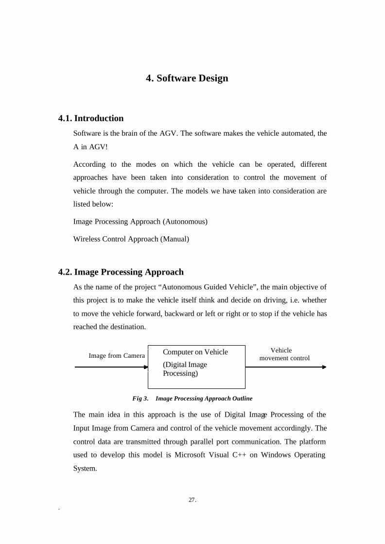
4.2. Image Processing Approach
As the name of the project “Autonomous Guided Vehicle”, the main objective of
this project is to make the vehicle itself think and decide on driving, i.e. whether
to move the vehicle forward, backward or left or right or to stop if the vehicle has
reached the destination.
Vehicle movement control
Computer on Vehicle
(Digital Image Processing)
Image from Camera
Fig 3. Image Processing Approach Outline
The main idea in this approach is the use of Digital Image Processing of the
Input Image from Camera and control of the vehicle movement accordingly. The
control data are transmitted through parallel port communication. The platform
used to develop this model is Microsoft Visual C++ on Windows Operating
System.

28. .
4.3. Digital Image Processing
A digital image is an array of real or complex numbers represented by a finite
numbers of bits.
The term digital image processing generally refers to processing of two-
dimensional picture by a digital computer. In other way, it can be said as digital
processing of any two-dimensional data. A typical digital image processing
sequence is shown in Figure 4.
Imaging System
Sample And Quantise
Storage (disk)
Digital Computer
Online Buffer Display
Record
Object Observe Digitize Store Process Refresh/ Store
Output
Fig 4. Digital Image Processing Sequence Block Diagram
Digital image processing has a broad spectrum of applications, such as remote
sensing via satellites and other spacecrafts, image transmission and storage for
business applications, medical processing, radar, sonar and acoustic image
processing, robotics and automated inspection of industrial parts. There many
image processing applications and problems as:
o Image representation and modeling
o Image enhancement
o Image analysis
o Image reconstruction
o Image data compression
In image representation one is concerned with characterization at the quantity
that each picture element (PIXEL or PEL) represents. An image could represent
luminance of objects in a scene (pictures taken by ordinary camera), the
absorption characteristics of the body tissue (X-ray imaging), the radar cross-
section of a target (radar imaging), etc.

29. .
In Image Enhancement, the goal is to accentuate certain image Features for
subsequent analysis or for image display. It includes, Contract and Edge Enhance
mar, pseudo coloring, noise filtering, sharpening and magnifying. It is useful in
Image analysis, Feature Extraction and visual information display.
Image analysis is concerned with making quantitative measurements from an
Image to produce a description of it. In the simplest form, this task could be
reading on a grocery item, sorting different parts on an assembly line, or
measur ing the size and orientation of blood cells in a medical Image. More
advanced image analysis system measure quantitative information and use it to
make a sophisticated decision, such as controlling the arm of a robot to move an
after identifying it or navigating an aircraft with aid of images acquired along its
trajectory.
Image reconstruction from projections is a special class of image restoration
problems where a two-(or higher) dimensional object is reconstructed from
several one-dimensional projections.
4.4. Image Acquisition
4.4.1. Preliminaries
The image is acquired through a sensor in the video camera known as the CCD.
CCD is a collection of tiny light-sensitive diodes, which convert photons (light)
into electrons (electrical charge). These diodes are called pho tosites. In a
nutshell, each photosite is sensitive to light - the brighter the light that hits a
single photosite, the greater the electrical charge that will accumulate at that site.
The CCD is the central element in an imaging system. Designers need to be
aware of the special requirements for the signal conditioning of the CCD in order
to achieve the maximum performance. The output signal of the CCD is a
constant stream of the individual pixel “charges” and this result in the typical
form of stepped DC voltage levels. This output signal also contains a DC-bias
voltage, which is in the order of several volts. The next stage is used as a noise
30. .
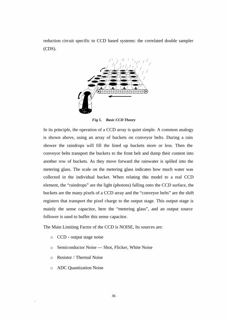
reduction circuit specific to CCD based systems: the correlated double sampler
(CDS).
Fig 5. Basic CCD Theory
In its principle, the operation of a CCD array is quiet simple. A common analogy
is shown above, using an array of buckets on conveyor belts. During a rain
shower the raindrops will fill the lined up buckets more or less. Then the
conveyor belts transport the buckets to the front belt and dump their content into
another row of buckets. As they move forward the rainwater is spilled into the
metering glass. The scale on the metering glass indicates how much water was
collected in the individual bucket. When relating this model to a real CCD
element, the “raindrops” are the light (photons) falling onto the CCD surface, the
buckets are the many pixels of a CCD array and the “conveyor belts” are the shift
registers that transport the pixel charge to the output stage. This output stage is
mainly the sense capacitor, here the “metering glass”, and an output source
follower is used to buffer this sense capacitor.
The Main Limiting Factor of the CCD is NOISE, Its sources are:
o CCD - output stage noise
o Semiconductor Noise — Shot, Flicker, White Noise
o Resistor / Thermal Noise
o ADC Quantization Noise

31. .
4.4.2. Camera components
The word camera comes from the term camera obscura. Camera means room (or
chamber) and obscura means dark. In other words, a camera is a dark room. This
dark room keeps out all unwanted light. At the click of a button, it allows a
controlled amount of light to enter through an opening and focuses the light onto
a sensor (either film or digital).
Aperture
The aperture is the size of the opening in the camera. It's located behind the lens.
On a bright sunny day, the light reflected from the image may be very intense,
and it doesn't take very much of it to create a good picture. In this situation, a
small aperture is required. But on a cloudy day, or in twilight, the light is not so
intense and the camera will need more light to create an image. In order to allow
more light, the aperture must be enlarged.
Shutter Speed
Traditionally, the shutter speed is the amount of time that light is allowed to pass
through the aperture. Think of a mechanical shutter as a window shade. It is
placed across the back of the aperture to block out the light. Then, for a fixed
amount of time, it opens and closes. The amount of time it is open is the shutter
speed. One way of getting more light into the camera is to decrease the shutter
speed. In other words, leave the shutter open for a longer period of time.
Film-based cameras must have a mechanical shutter. Once film is exposed to
light, it can't be wiped clean to start again. Therefore, it must be protected from
unwanted light. But the sensor in a digital camera can be reset electronically and
used over and over again. This is called a digital shutter. Some digital cameras
employ a combination of electrical and mechanical shutters.
Exposing the Sensor
These two aspects of a camera, aperture and shutter speed, work together to
capture the proper amount of light needed to make a good image. In
photographic terms, they set the exposure of the sensor. Most digital cameras

32. .
automatically set aperture and shutter speed for optimal exposure, which gives
them the appeal of a point-and-shoot camera.
Lens and Focal Length
A camera lens collects the available light and focuses it on the sensor. The focal
length is the distance between the lens and the surface of the sensor. Technical
details show that the surface of a film sensor is much larger than the surface of a
CCD sensor. In fact, a typical 1.3 mega-pixel digital sensor is approximately
one-sixth of the linear dimensions of film. In order to project the image onto a
smaller sensor, it is necessary to shorten the focal length by the same proportion.
Focal length is also the critical information in determining how much
magnification we get when we look through the camera. In 35 mm cameras, a 50
mm lens gives a natural view of the subject. As the focal length is increased, we
get greater magnification and objects appear to get closer. As we decrease the
focal length, things appear to get further away, but we can capture a wider field
of view in the camera.
4.4.3. Camera solution to obtain intensity images
Camera (can be assumed as digital) has a sensor that converts light into electrical
charges. All the fun and interesting features of digital cameras come as a direct
result of this shift from recording an image on film to recording the image in
digital form.
The image sensor employed by most digital cameras is a charge-coupled device
(CCD). Some low-end cameras use complementary metal oxide semiconductor
(CMOS) technology. While CMOS sensors will almost certainly improve and
become more popular in the future, they probably won't replace CCD sensors in
higher-end digital cameras.
How the Camera Captures Color?
Unfortunately, each photosite is colorblind. It only keeps track of the total
intensity of the light that strikes its surface. In order to get a full color image,
most sensors use filtering to look at the light in its three primary colors. Once all
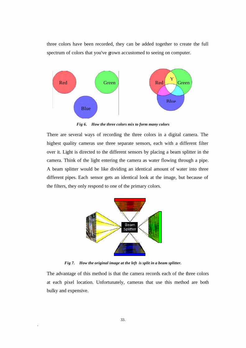
33. .
three colors have been recorded, they can be added together to create the full
spectrum of colors that you've grown accustomed to seeing on computer.
Blue
Green Red
Blue
Red Green Y
Fig 6. How the three colors mix to form many colors
There are several ways of recording the three colors in a digital camera. The
highest quality cameras use three separate sensors, each with a different filter
over it. Light is directed to the different sensors by placing a beam splitter in the
camera. Think of the light entering the camera as water flowing through a pipe.
A beam splitter would be like dividing an identical amount of water into three
different pipes. Each sensor gets an identical look at the image, but because of
the filters, they only respond to one of the primary colors.
Fig 7. How the original image at the left is split in a beam splitter.
The advantage of this method is that the camera records each of the three colors
at each pixel location. Unfortunately, cameras that use this method are both
bulky and expensive.

34. .
A second method is to rotate a series of red, blue and green filters in front of a
single sensor. The sensor records three separate images in rapid succession. This
method also provides information on all three colors at each pixel location. But
since the three images aren't taken at precisely the same moment, both the
camera and the target of the photo must remain stationary for all three readings.
This isn't practical for candid photography or handheld cameras.
Fig 8. A spinning disk filter.
A more economical and practical way to record the three primary colors from a
single image is to permanently place a filter over each individual photosite. By
breaking up the sensor into a variety of red, blue and green pixels, it is possible
to get enough information in the general vicinity of each sensor to make very
accurate guesses about the true color at that location. This process of looking at
the other pixels in the neighborhood of a sensor and making an educated guess is
called interpolation. (You'll learn more about pixels in the next section, but for
now, think of one photosite as a single pixel.)
Frame buffer
A frame buffer device is an abstraction for the graphic hardware. It represents the
frame buffer of some video hardware, and allows application software to access
the graphic hardware through a well-defined interface, so that the software
doesn't need to know anything about the low-level interface stuff.
The major advantage of the frame buffer drives is that it presents a generic
interface across all platforms.

35. .
Intensity Images
Intensity images measure the amount of light impinging on a photosensitive
device. The input to the photosensitive device, typically a camera, is the
incoming light, which enters the camera's lens and hits the image plane. In a
digital camera, the physical image plane is an array which contains a rectangular
grid of photo sensors, each sensitive to light intensity. The output of the array is a
continuous electric signal, the video signal. The video signal is sent to an
electronic device called frame grabber, where it is digitized into a 2D rectangular
array of integer values and stored in a memory buffer.
The interpretation of an intensity image depends strongly on the characteristics
of the camera called the camera parameters. The parameters can be separated
into extrinsic and intrinsic parameters.
The extrinsic parameters transform the camera reference frame to the world
reference frame. These are the parameters that define the location and orientation
of the camera reference frame with respect to a known world reference frame
The intrinsic parameters describe the optical, geometric and digital
characteristics of the camera. One parameter, for example, can describe the
geometric distortion introduced by the optics. So, these are the parameters
necessary to link the pixel coordinates of an image point with the corresponding
coordinates in the camera reference frame.
4.5. Camera parameters and calibration
4.5.1. Basic Optics
We first need to establish a few fundamental notions of optics. As for many
natural visual systems, the process of image formation in computer vision begins
with the light rays which enter the camera through an angular aperture (or pupil),
and hit a screen or image plane, the camera’s photosensitive device which
registers light intensities. Notice that most of these rays are the result of the
reflections of the rays emitted by the light sources and hitting object surfaces.

36. .
Fig 9. The basic element of an Imaging System
4.5.2. Image Focusing
Any single point of a scene reflects light coming from possibly many directions,
so that many rays reflected by the same point may enter the camera. In order to
obtain sharp images, all rays coming from a single scene point, P, must converge
onto a single point on the image plane, p, the image of P. If this happen, we say
that the image of P is in focus; if not, the image is spread over a circle. Focusing
all rays from a scene point onto a single image point can be achieved in two
ways:
Reducing the camera’s aperture to a point is called a pinhole. This means that
only one ray from any given point can enter the camera, and creates a one-to-one
correspondence between visible points, rays and image points. This results in
very sharp, undistorted images of objects at different distances from the camera.
Introducing an optical system composed of lenses, apertures, and other elements,
explicitly designed to make all rays coming from the same 3-D point converge
onto a single image point.
An obvious disadvantage of a pinhole aperture is its exposure time; that is, how
long the image plane is allowed to receive light. Any photosensitive device
(camera film, electronic sensors) needs a minimum amount of light to register a
legible image. As a pinhole allows very little light into the camera per time unit,

37. .
the exposure time necessary to form the image is too long (typically several
seconds) to be of practical use. (Note: The exposure time is, roughly, inversely
proportional to the square of the aperture diameter, which in turn is proportional
to the amount of light that enters the imaging system). Optical systems, instead,
can be adjusted to work under a wide range of illumination conditions and
exposure times (the exposure time being controlled by a shutter).
Intuitively, an optical system can be regarded as a device that aims at producing
the same image obtained by a pinhole aperture, but by means of a much larger
aperture and a shorter exposure time. Moreover, an optical system enhances the
light gathering power.
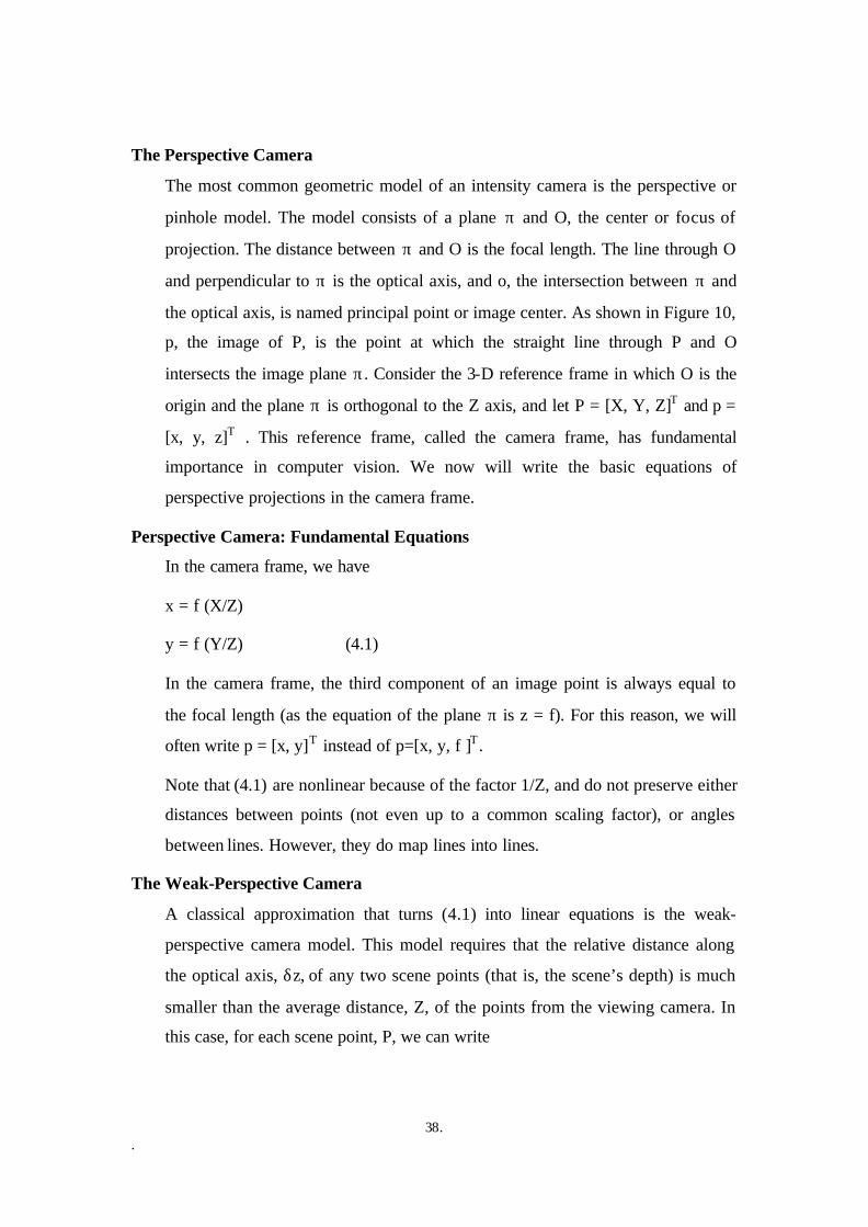
4.6. Geometric Image Formation
We now turn to the geometric aspect of image formation. The aim is to link the
position of scene points with that of their corresponding image points. To do this,
we need to model the geometric projection performed by the sensor.
Fig 10. The Perspective Camera Model.
38. .
The Perspective Camera
The most common geometric model of an intensity camera is the perspective or
pinhole model. The model consists of a plane π and O, the center or focus of
projection. The distance between π and O is the focal length. The line through O
and perpendicular to π is the optical axis, and o, the intersection between π and
the optical axis, is named principal point or image center. As shown in Figure 10,
p, the image of P, is the point at which the straight line through P and O
intersects the image plane π . Consider the 3-D reference frame in which O is the
origin and the plane π is orthogonal to the Z axis, and let P = [X, Y, Z]T and p =
[x, y, z]T . This reference frame, called the camera frame, has fundamental
importance in computer vision. We now will write the basic equations of
perspective projections in the camera frame.
Perspective Camera: Fundamental Equations
In the camera frame, we have
x = f (X/Z)
y = f (Y/Z) (4.1)
In the camera frame, the third component of an image point is always equal to
the focal length (as the equation of the plane π is z = f). For this reason, we will
often write p = [x, y]T instead of p=[x, y, f ]T .
Note that (4.1) are nonlinear because of the factor 1/Z, and do not preserve either
distances between points (not even up to a common scaling factor), or angles
between lines. However, they do map lines into lines.
The Weak-Perspective Camera
A classical approximation that turns (4.1) into linear equations is the weak-
perspective camera model. This model requires that the relative distance along
the optical axis, δz, of any two scene points (that is, the scene’s depth) is much
smaller than the average distance, Z, of the points from the viewing camera. In
this case, for each scene point, P, we can write
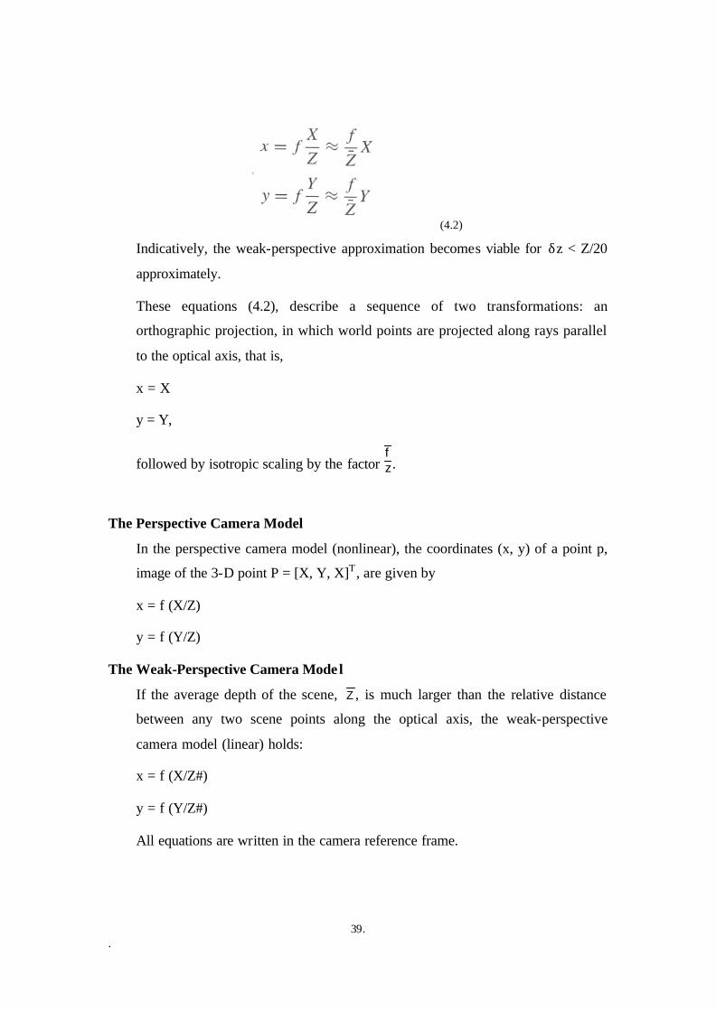
39. .
(4.2)
Indicatively, the weak-perspective approximation becomes viable for δz < Z/20
approximately.
These equations (4.2), describe a sequence of two transformations: an
orthographic projection, in which world points are projected along rays parallel
to the optical axis, that is,
x = X
y = Y,
followed by isotropic scaling by the factor zf.
The Perspective Camera Model
In the perspective camera model (nonlinear), the coordinates (x, y) of a point p,
image of the 3-D point P = [X, Y, X]T , are given by
x = f (X/Z)
y = f (Y/Z)
The Weak-Perspective Camera Mode l
If the average depth of the scene, Z, is much larger than the relative distance
between any two scene points along the optical axis, the weak-perspective
camera model (linear) holds:
x = f (X/Z#)
y = f (Y/Z#)
All equations are written in the camera reference frame.

40. .
4.7. Camera Parameters
We now come back to discuss the geometry of a vision system in greater detail.
In particular, we want to characterize the parameters underlying camera models.
Definitions
Computer vision algorithms reconstructing the 3-D structure of a scene or
computing the position of objects in space need equations linking the coordinates
of points in 3-D space with the coordinates of their corresponding image points.
These equations are written in the camera reference frame (4.1), but it is often
assumed that
The camera reference frame can be located with respect to some other, known,
reference frame (the world reference frame), and
The coordinates of the image points in the camera reference frame can be
obtained from pixel coordinates, the only ones directly available from the
images.
This is equivalent to assume knowledge of some camera’s characteristics, known
in vision as the camera’s extrinsic and intrinsic parameters. Our next task is to
understand the exact nature of the intrinsic and extrinsic parameters and why the
equivalence holds.
Camera Parameters
The extrinsic parameters are the parameters that define the location and
orientation of the camera reference frame with respect to a known world
reference frame.
The intrinsic parameters are the parameters necessary to link the pixel
coordinates of an image point with the corresponding coordinates in the camera
reference frame.
We now try to write the basic equations that allow us to define the extrinsic and
intrinsic parameters in practical terms. The problem of estimating the value of
these parameters is called camera calibration.

41. .
Extrinsic Parameters
The camera reference frame has been introduced for the purpose of writing the
fundamental equations of the perspective projection (4.1) in a simple form.
However, the camera reference frame is often unknown, and a common problem
is determining the location and orientation of the camera frame with respect to
some known reference frame, using only image information. The extrinsic
parameters are defined as any set of geometric parameters that identify uniquely
the transformation between the unknown camera reference frame and a known
reference frame.
A typical choice for describing the transformation between camera and world
frame is to use
A 3-D translation vector, T, describing the relative positions of the origins of the
two reference frames, and
A 3 X 3 rotation matrix, R, an orthogonal matrix (RTR = RRT = I) that brings the
corresponding axes of the two frames onto each other.
Fig 11. The Relation between camera and world coordinate frames
The orthogonality relations reduce the number of degrees of freedom of R to
three.

42. .
In an obvious notation (see Figure 11), the relation between the coordinates of a
point P in world and camera frame, Pw and Pc respectively, is
Pw = R(Pc – T), (4.3)
With
Extrinsic Parameters
The camera extrinsic parameters are the translation vector, T, and the rotation
matrix, R (or, better, its free parameters), which specify the transformation
between the camera and the world reference frame.
4.8. Intrinsic Parameters
The intrinsic parameters can be defined as the set of parameters needed to
characterize the optical, geometric, and digital characteristics of the viewing
camera. For a pinhole camera, we need three sets of intrinsic parameters,
specifying respectively
The perspective projection, for which the only parameter is the focal length, f;
The transformation between camera frame coordinates and pixel coordinates;
The geometric distortion introduced by the optics.
From Camera to Pixel Coordinates
To find the second set of intrinsic parameters, we must link the coordinates (xim ,
yim) of an image point in pixel units with the coordinates (x, y) of the same point
in the camera reference frame. The coordinates (xim, yim) can be thought of as
coordinates of a new reference frame, sometimes called image reference frame.
43. .
Transformation between Camera and Image Frame Coordinates
Neglecting any geometric distortions possibly introduced by the optics and in the
assumption that the CCD array is made of a rectangular grid of photosensitive
elements, we have
x = - (xim - ox) sx
y = - (yim - oy) sy (4.4)
with (ox,oy) the coordinates in pixel of the image center (the principal point), and
(sx,sy) the effective size of the pixel (in millimeters) in the horizontal and vertical
direction respectively.
Therefore, the current set of intrinsic parameters is f, ox , oy, sx , sy,.
The sign change in (4.4) is due to the fact that the horizontal and vertical axes of
the image and camera reference frames have opposite orientation.
In several cases, the optics introduces image distortions that become evident at
the periphery of the image, or even elsewhere using optics with large fields of
view. Fortunately, these distortions can be modeled rather accurately as simple
radial distortions, according to the relations
x = xd(1 + k1r2 + k2r4)
y = yd (1 + k1r2 + k2r4)
with (xd , yd) the coordinates of the distorted points, and r2 = x d2 + y d2 . As
shown by the equations above, this distortion is a radial displacement of the
image points. The displacement is null at the image center, and increases with the
distance of the point from the image center. k1 and k2 are further intrinsic
parameters. Since they are usually very small, radial distortion is ignored
whenever high accuracy is not required in all regions of the image, or when the
peripheral pixels can be discarded. If not, as k2 << k1, k2 is often set equal to 0,
and k1 is the only intrinsic parameter to be estimated in the radial distortion
model.
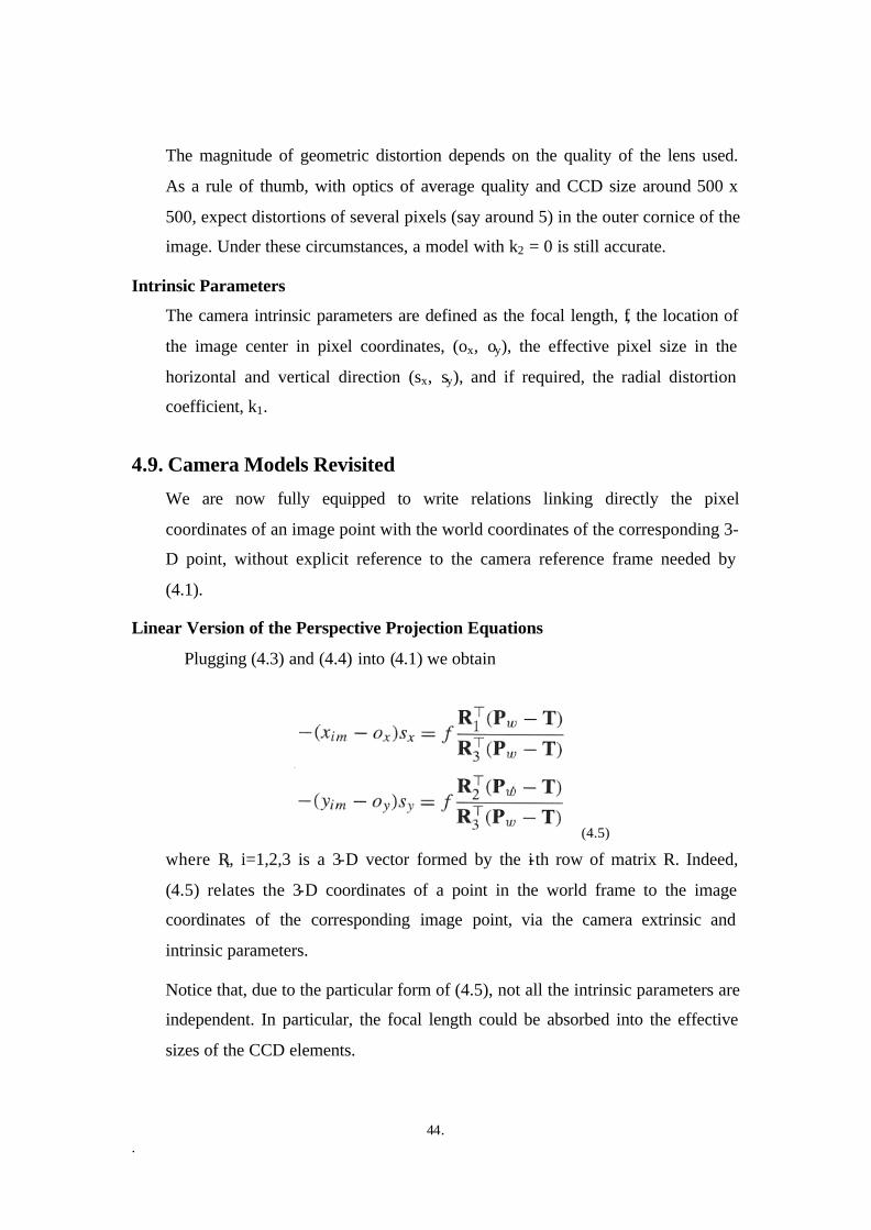
44. .
The magnitude of geometric distortion depends on the quality of the lens used.
As a rule of thumb, with optics of average quality and CCD size around 500 x
500, expect distortions of several pixels (say around 5) in the outer cornice of the
image. Under these circumstances, a model with k2 = 0 is still accurate.
Intrinsic Parameters
The camera intrinsic parameters are defined as the focal length, f, the location of
the image center in pixel coordinates, (ox, oy), the effective pixel size in the
horizontal and vertical direction (sx, sy), and if required, the radial distortion
coefficient, k1.
4.9. Camera Models Revisited
We are now fully equipped to write relations linking directly the pixel
coordinates of an image point with the world coordinates of the corresponding 3-
D point, without explicit reference to the camera reference frame needed by
(4.1).
Linear Version of the Perspective Projection Equations
Plugging (4.3) and (4.4) into (4.1) we obtain
(4.5)
where Ri, i=1,2,3 is a 3-D vector formed by the i-th row of matrix R. Indeed,
(4.5) relates the 3-D coordinates of a point in the world frame to the image
coordinates of the corresponding image point, via the camera extrinsic and
intrinsic parameters.
Notice that, due to the particular form of (4.5), not all the intrinsic parameters are
independent. In particular, the focal length could be absorbed into the effective
sizes of the CCD elements.

45. .
Neglecting radial distortion, we can rewrite (4.5) as a simple matrix product.
To this purpose, we define two matrices, Mint and Mext, as
so that the 3 x 3 matrix Mint depends only on the intrinsic parameters, while the
3 x 4 matrix Mext only on the extrinsic parameters. If we now add a “1” as a
fourth coordinate of (that is, express in homogeneous coordinates), and form the
product Mext, we obtain a linear matrix equation describing perspective
projections.
The Linear Matrix Equation of Perspective Projections
What is interesting about vector [x1, x2, x3]T is that the ratios and are
nothing but the image coordinates:
x1/x3 = xim
x2/x3 = yim
Moreover, we have separated nicely the two steps of the world- image projection:
Mext performs the transformation between the world and the camera reference
frame;
Mint performs the transformation between the camera reference frame and the
image reference frame.
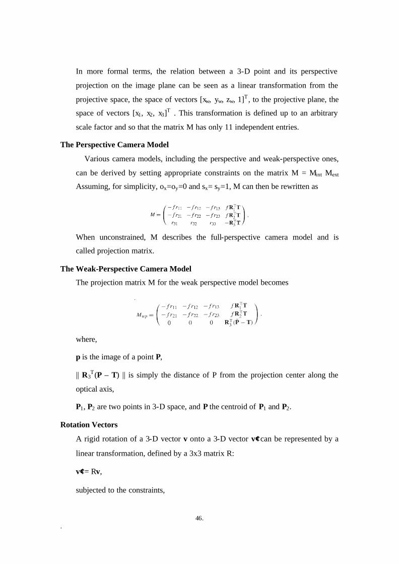
46. .
In more formal terms, the relation between a 3-D point and its perspective
projection on the image plane can be seen as a linear transformation from the
projective space, the space of vectors [xw, yw, zw, 1]T , to the projective plane, the
space of vectors [x1, x2, x3]T . This transformation is defined up to an arbitrary
scale factor and so that the matrix M has only 11 independent entries.
The Perspective Camera Model
Various camera models, including the perspective and weak-perspective ones,
can be derived by setting appropriate constraints on the matrix M = Mint Mext
Assuming, for simplicity, ox=oy=0 and sx= sy=1, M can then be rewritten as
When unconstrained, M describes the full-perspective camera model and is
called projection matrix.
The Weak-Perspective Camera Model
The projection matrix M for the weak perspective model becomes
where,
p is the image of a point P,
|| R3T(P – T) || is simply the distance of P from the projection center along the
optical axis,
P1, P2 are two points in 3-D space, and P the centroid of P1 and P2.
Rotation Vectors
A rigid rotation of a 3-D vector v onto a 3-D vector v′′ can be represented by a
linear transformation, defined by a 3x3 matrix R:
v′′ = Rv,
subjected to the constraints,

47. .
RRT = RTR = I det(R) = 1,
with ‘I’ the identity matrix. The first constraint tells that the inverse of R equal its
transpose. The second that the transformation preserves the relative orientation of
the reference frame, and therefore its right- or left-handedness.
A matrix R for which RRT = I is called orthogonal. The orthogonality property
can be better appreciated by assuming that v and v′ are expressed in two
orthogonal references frames, defined by the unit vectors e1, e2, e3, and e1′, e2′, e3′
respectively. It can easily be seen that the generic entry rij of R is the cosine of
the angle formed by the base vector, eim with the rotated base vector e′j:
rij = eiTe′j
Therefore, we have that
that is, the rows (and columns) of r are mutually orthogonal unit vectors. But
even a slight perturbation of the entries of R, due to noise or small errors,
destroys the orthogonality property and affects the estimation of the rotation
parameters.
Two Useful Parameterizations
A 3x3 orthogonal matrix has nine elements which have to satisfy the six
orthogonality constraints. This reduces the number of degrees of freedom of a 3-
D rotation to 9-6=3 and tells that describing a rotation matrix through its nine
entries is redundant and not really natural; in most cases it is useful and simpler
to represent a rotation by means of more natural parameterization. We limit
ourselves to the two parameterizations used in the book: rotations around the
coordinate axes and axis and angle.
Rotations around the Coordinate Axes
We can express a 3-D rotation as the result of three consecutive rotations around
the coordinate axes e1, e2, and e3, by angles α, β, and γ respectively. The angles
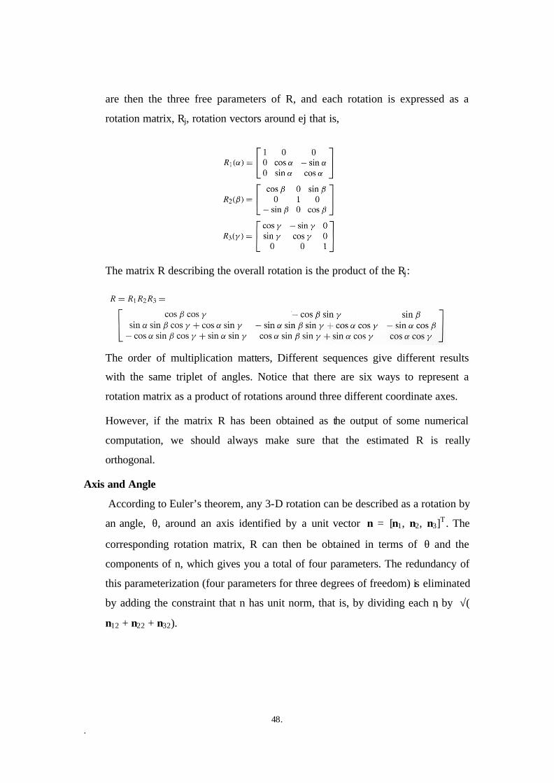
48. .
are then the three free parameters of R, and each rotation is expressed as a
rotation matrix, Rj, rotation vectors around ej that is,
The matrix R describing the overall rotation is the product of the Rj:
The order of multiplication matters, Different sequences give different results
with the same triplet of angles. Notice that there are six ways to represent a
rotation matrix as a product of rotations around three different coordinate axes.
However, if the matrix R has been obtained as the output of some numerical
computation, we should always make sure that the estimated R is really
orthogonal.
Axis and Angle
According to Euler’s theorem, any 3-D rotation can be described as a rotation by
an angle, θ, around an axis identified by a unit vector n = [n1, n2, n3]T . The
corresponding rotation matrix, R can then be obtained in terms of θ and the
components of n, which gives you a total of four parameters. The redundancy of
this parameterization (four parameters for three degrees of freedom) is eliminated
by adding the constraint that n has unit norm, that is, by dividing each ni by √(
n12 + n22 + n32).

49. .
The matrix R in terms of θ and n is given by
4.10. Noise Theory
The effect of noise is, essentially, that image values are not those expected, as
these are corrupted during the various stages of image acquisition. As a
consequence, the pixel values of two images of the same scene taken by the same
camera and in the same light conditions are never exactly the same. Such
fluctuations will introduce errors in the results of calculations based on pixel
values; it is therefore important to estimate the magnitude of the noise.
Another cause of noise, which is important when a vision system is used for fine
measurements, is that pixel values are not completely independent of each other.
Some cross talking occurs between adjacent photo sensors in each row of the
CCD array, due to the way the content of each CCD row is read in order to be
sent to the frame buffer. This can be verified by computing the auto covariance
CEE(i, j) of the image of a spatially uniform pattern parallel to the image plane
and illuminated by diffuse light.
In computer vision, noise may refer to any entity, in images, data or intermediate
results, which is not interesting for the purpose of the main computation.
4.10.1. Image Noise
The main image noise is additive and random; that is a spurious, random signal,
n(i, j), added to the true pixel values I(i, j):
I’(i, j) = I(i, j) + n(i, j)
4.10.2. Noise Amount
The amount of noise in an image can be estimated by means of σn, the standard
deviation of the random signal n(i, j). It is important to know how strong the

50. .
noise is with respect to the interesting signal. This is specified by the signal- to-
noise ratio (SNR).
n
sS N Rσσ=
Where σs is the standard deviation of the signal (the pixel values I(i, j)). The
SNR is often expressed in decibel:
n
sdbSNR
σσ
10log10=
4.10.3. Gaussian Noise
In the absence of information, one often assumes n(i,j) to be modeled by a white,
Gaussian, zero-mean stochastic process. For each location (i, j), this amounts to
thinking of n( i, j) as random variables distributed according to a zero mean
Gaussian distribution function of fixed standard deviation, which is added to I(i,
j) and whose values are completely independent of each other and of the image in
both space and time.
4.10.4. Impulsive Noise
Impulsive Noise, also known as spot or peak noise, occurs usually in addition to
the one normally introduced by acquisition. Impulsive noise alters random pixels,
making their values very different from the true values and very often from those
of neighboring pixels too. Impulsive noise appears in the image as a sprinkle of
dark and light spots. It can be caused by transmission errors, faulty elements in
the CCD array, or external noise corrupting the analog-to-digital conversion.

51. .
4.11. Block diagram of image processing model
POP AN IMAGE FROM SEQUENCE
GET SUB IMAGE
EDGE DETECTION
HOUGH TRANSFORM
NEXT DECISION ? (i.e. DRIVE LEFT OR
RIGHT OR STOP)
OUTPUT: CONTROL DATA TO
CIRCUIT
INPUT: IMAGE SEQUENCE FROM
CAMERA
Fig 12. Block Diagram of Software model (Image Processing Approach)
4.12. Image Analysis
The ultimate aim in a large number of image processing applications is to extract
important features from image data, from which a description, interpretation, or
understanding of the scene can be provided by the machine. Image analysis

52. .
basically involves the study of feature extraction, segmentation and classification
techniques.
Image Analysis Techniques
Feature Extraction
• Spatial Features • Transform Features • Edge & Boundaries • Shape Features • Moments • Texture
Segmentation
• Template Matching • Thresholding • Boundary Detection • Clustering • Quad - Trees • Texture Matching
Classification
• Clustering • Statistical • Decision Trees • Similarity Measures • Minimum Spanning
Trees
4.13. Edge Detection
How do edges come in an image? Probably, the answer to this question provides
the early importance clue for locating edges in an image. The variations of image
features, usually brightness, give rise to edges. More objectively, the edges are
the representations of the discontinuities of image intensity function. There could
be various reasons, such as lightening conditions, object(s) geometry, type of
material, surface texture, etc., as well as their mutual interactions, for the
discontinuities. Therefore, edge-detection algorithm is essentially a process of
detection of these discontinuities in an image. Since the abrupt changes in
brightness level indicates edge, its detection in binary or segmented image is
quite straightforward (such edges are called border or boundary). However, the
process of edge localization is quite complex in the case of gray level or intensity
level images. The transition in intensity in gray-scale image is relatively smooth
in nature rather than abrupt as in the case of segmented binary images. The
nature of intensity variation points to the application of derivative operators for
detecting edges. Application of derivative operators on intensity image produces
another image, usually called gradient image as it reveals the rate of intensity
variation. This image is made to undergo thresholding and/or edge linking in
53. .
order to yield contours. Thus, the image is decomposed into various regions
resulting in another kind of segmentation.
Edge points can be thought of as pixel locations of abrupt gray- level change. For
example, it is responsible to define edge points in binary images as black pixels
with at least one white nearest neighbor, that is, pixel locations (m, n) such that
u(m, n)=0 and g(m, n)=1; where
g(m, n) ⊕ [u(m, n) ⊕ u(m±1, n)] , OR
[u(m, n) ⊕ u(m,n±1)]
Where ⊕ denotes the logical exc lusives or operation. For a continuous image f(x,
y) its derivative assumes a local maximum in the direction of the Edge.
Therefore, one edge direction technique is to measure the gradient of f along r in
a direction è, that is,
ryyfrxxfrf ∂∂∂∂+∂∂∂∂=∂∂ **
θθ sincos yx ff +=
The maximum value of df/dr is obtained when (d/dϕ) df/dr)= 0. This gives
0cossin =+− gygx ff θθ
)(tan 1yxg ff−=θ
22max)( yx ffrf +=∂∂
Where ϕg is the direction of the edge.
Based on these concepts, two types of edge detection operators have been
introduced:
o Gradient Operators
o Compass Operators
For digital images these operators, are also called masks, represent finite
difference approximations of either the orthogonal gradients fx, fy or the

54. .
directional gradient df/dx. Let H denote a P x P mask and define, for an arbitrary
image U, their inner product at location (m, n) as the correlation.
∑∑ ⊕=++≅><i j
nm hnmunjmiujihHU ),(),(),(, ,
4.13.1. Gradients Operators
These are represented by a pair of marks h1, h2 which measure the gradient of the
image u(m,n) in two orthogonal directions. Defining the bi-directional gradients
g1(m1)= <U,H1>m,n , g1(m)= <U,H2>m,n the gradient vector magnitude and
direction are given by:
g(m,n)= √g12 (m,n)+ g2
2 (m,n)
èg (m,n) = tan-1(g2(m,n) / g1(m,n))
h1(-m,-n)
h2(-m,-n)
g=√ g12+g2
2 èg=tan- 1 (y2/y1)
1 0 Threshold
Direction èg (m,n) Edge map
u(m,n)
Fig 13. Edge detection via gradient operator
Rather than the above equation the magnitude gradient is calculated by:
g(m,n) = | g1(m,n) | + | g2(m,n) |
Some of the gradient operator are shown below:

55. .
H1 H2 0 1 1 0 Roberts
-1 0
0 -1
-1 0 1 -1 -1 -1 -1 0 1 0 0 0
Smoothed Prewitt
-1 0 1 1 1 1
-1 0 1 -1 -2 -1 Sobel -2 0 2 0 0 0
-1 0 1 1 2 1
-1 0 1 -1
2− -1 Isotrope
2−
0 2
0 0 0
-1 0 1 1
2
1
4.13.2. Compass operators
Compass operators measure gradients in a selected number of directions
èk
hk (-m,-n) 1 0 Threshold
Edge map
u(m,n) g (m,n) Max k{1,1}
g (m,n)
Fig 14. Edge detection via compass operator
56. .
4.14. The Hough Transform
The Hough transform is a technique, which can be used to isolate features of a
particular shape within an image.
Because it requires that the desired features be specified in some parametric
form, the classical Hough trans form is most commonly used for the detection of
regular curves such as lines, circles, ellipses, etc.
A generalized Hough transform can be employed in applications where a simple
analytic description of a feature(s) is not possible.
The Hough transform has many applications, as most manufactured parts (and
many anatomical parts investigated in medical imagery) contain feature
boundaries, which can be described by regular curves or straight lines.
The main advantage of the Hough transform is that it is tolerant of gaps in
feature boundary descriptions and is relatively unaffected by image noise.
4.14.1. Working Principle of Hough Transform
The Hough technique is useful for computing a global description of a feature(s)
(where the number of solution classes need not be known a priori), given
(possibly noisy) local measurements.
The motivating idea behind the Hough technique for line detection is that each
input measurement (e.g. coordinate point) indicates its contribution to a globally
consistent solution (e.g. the physical line which gave rise to that image point).
As a simple example, consider the common problem of fitting a set of line
segments to a set of discrete image points (e.g. pixel locations output from an
edge detector). The diagram below shows some possible solutions to this
problem.
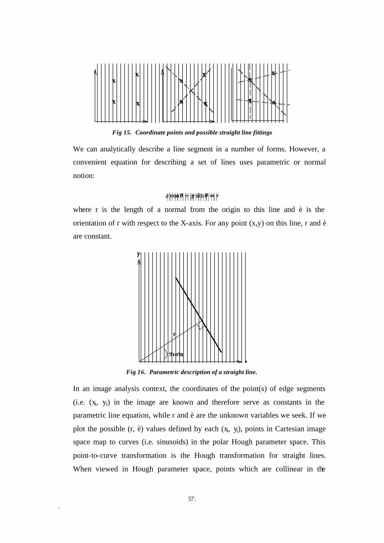
57. .
Fig 15. Coordinate points and possible straight line fittings
We can analytically describe a line segment in a number of forms. However, a
convenient equation for describing a set of lines uses parametric or normal
notion:
where r is the length of a normal from the origin to this line and è is the
orientation of r with respect to the X-axis. For any point (x,y) on this line, r and è
are constant.
Fig 16. Parametric description of a straight line.
In an image analysis context, the coordinates of the point(s) of edge segments
(i.e. (xi, yi) in the image are known and therefore serve as constants in the
parametric line equation, while r and è are the unknown variables we seek. If we
plot the possible (r, è) values defined by each (xi, yi), points in Cartesian image
space map to curves (i.e. sinusoids) in the polar Hough parameter space. This
point-to-curve transformation is the Hough transformation for straight lines.
When viewed in Hough parameter space, points which are collinear in the

58. .
Cartesian image space become readily apparent as they yield curves which
intersect at a common (r, è) point.
The transform is implemented by quantizing the Hough parameter space into
finite intervals or accumulator cells. (i.e. a multidimensional array). As the
algorithm runs, each (xi, yi) is transformed into a discretized (r, è) curve and the
accumulator cells which lie along this curve are incremented.
Peaks in the accumulator array represent strong evidence that a corresponding
straight line exists in the image.
We can use this same procedure to detect other features with analytical
descriptions. For instance, in the case of circles, the parametric equation is
Where a and b are the coordinates of the center of the circle and r is the radius. In
this case, the computational complexity of the algorithm begins to increase as we
now have three coordinates in the parameter space and a 3-D accumulator. (In
general, the computation and the size of the accumulator array increase
polynomially with the number of parameters. Thus, the basic Hough technique
described here is only practical for simple curves.)
The Hough transform can be used to identify the parameter(s) of a curve, which
best fits a set of given edge points.
This edge description is commonly obtained by using an edge detector such as
the zero crossings of the Laplacian. The edge image may be noisy, i.e. it may
contain multiple edge fragments corresponding to a single whole feature.
Since the output of an edge detector defines only where features are in an image,
the work of the Hough transform is to determine both what the features are (i.e.
to detect the feature(s) for which it has a parametric description) and how many
of them exist in the image.
In order to illustrate the Hough transform in detail, we begin with the simple
image of two occluding rectangles,

59. .
An edge detector can produce a set of boundary descriptions for this part, as
shown below
Fig 17. Original and Edge Detected Image
Here we see the overall boundaries in the image, but this result tells us nothing
about the identity (and quantity) of feature(s) within this boundary description. In
this case, we can use the Hough (line detecting) transform to detect the eight
separate straight lines segments of this image and thereby identify the true
geometric structure of the subject.
If we use these edge/boundary points as input to the Hough transform, a curve is
generated in polar (r, è) space for each edge point in Cartesian space. The
accumulator array, when viewed as an intensity image, looks like
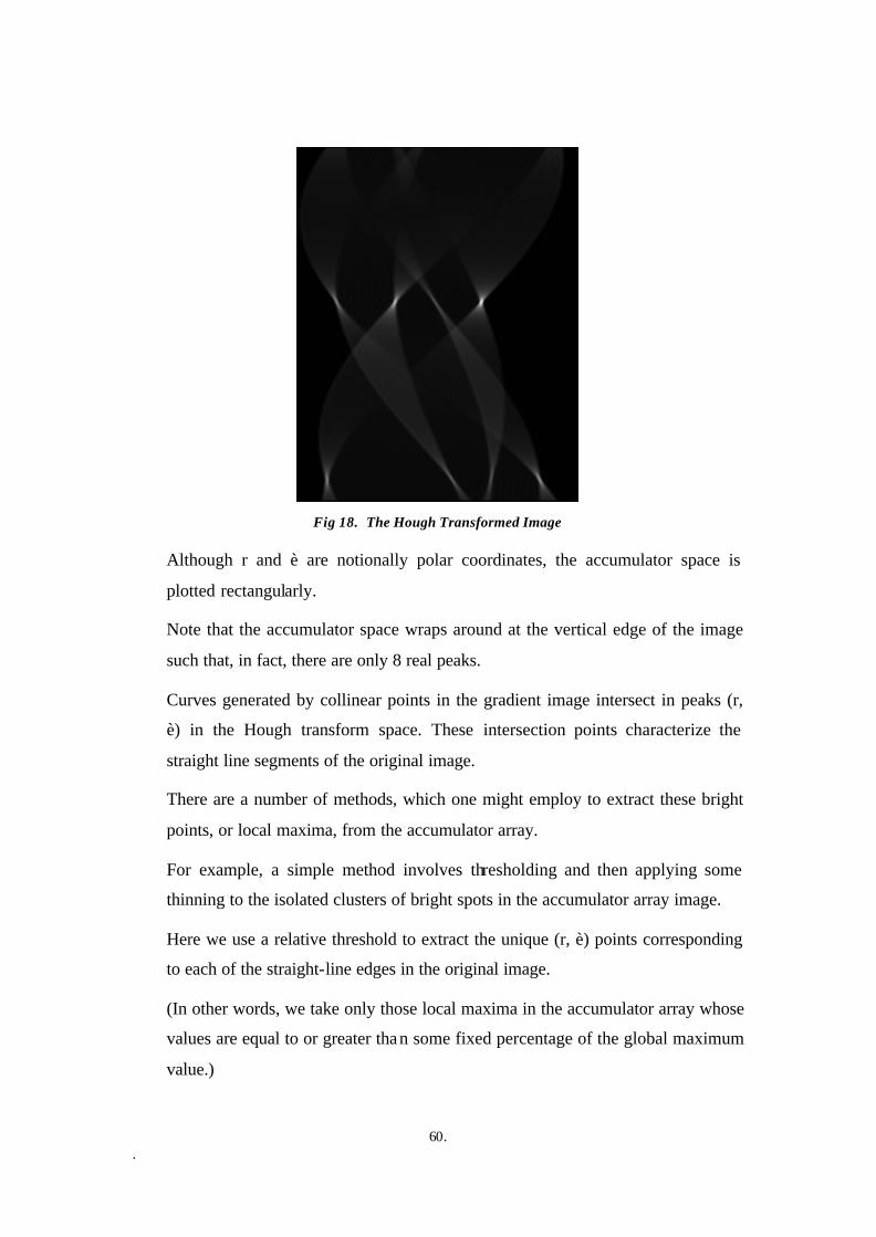
60. .
Fig 18. The Hough Transformed Image
Although r and è are notionally polar coordinates, the accumulator space is
plotted rectangularly.
Note that the accumulator space wraps around at the vertical edge of the image
such that, in fact, there are only 8 real peaks.
Curves generated by collinear points in the gradient image intersect in peaks (r,
è) in the Hough transform space. These intersection points characterize the
straight line segments of the original image.
There are a number of methods, which one might employ to extract these bright
points, or local maxima, from the accumulator array.
For example, a simple method involves thresholding and then applying some
thinning to the isolated clusters of bright spots in the accumulator array image.
Here we use a relative threshold to extract the unique (r, è) points corresponding
to each of the straight-line edges in the original image.
(In other words, we take only those local maxima in the accumulator array whose
values are equal to or greater than some fixed percentage of the global maximum
value.)
61. .
4.15. Platform Used: Microsoft Visual C++
Visual C++ is a powerful and a complex tool for building 32-bit application for
Windows 95 and Windows NT, including database application, Internet
application, application that taps the power of the ActiveX technology. These
applications are larger and more complex than their predecessor for 16-bit
Windows or older programs that didn't use a graphical interface. Yet, as a
program size and complexity has increased, programmer effort has decreased at
least for the programmers who are using the right tools.
Visual C++ is one of the right tools with its code-generating wizard, it can
produce the shell of the working Windows application in seconds. The class
library included with Visual C++, the Microsoft foundation classes [MFC], has
become industry standard for Windows software development in a variety of
C++ compilers. The visual editing tools make layout of menus and dialog a snap.
Microsoft Visual C++ is one component of the Microsoft developer Studio. It is
called an Integrated Development Environment [IDE] because within a single
tool, it can perform the following:
o Generate starter applications without writing code.
o View a project in several different ways.
o Edit sources and include files.
o Build the visual interface of your application.
o Compile and link.
o Debug an application when it runs.
In general, Visual C++ does not just compile code but it generates code too. It
can create Windows Applications with a very effective tool called AppWizard
that copies into your application the code that almost all Windows Application
requires, thus building a variety of Windows Applications.

62. .
4.16. Image Processing Libraries
There are many Image Processing libraries available that can be used for image
processing, some of which are discussed below:
4.16.1. Intel OpenCV
This open-source computer vision software library is a beautiful offering and has
a dedicated user group. Frustrating however is that it has compile bugs, code is
not well-documented and some examples rely on compiled object code or
DirectX. Those comfortable with DirectX, MFC and Win32 API can perhaps
debug and develop applications. Those without such experience will find the
learning curve very steep.
4.16.2. Microsoft Vision SDK
The Microsoft Vision SDK is a library for writing programs to perform image
manipulation and analysis on computers running Microsoft Windows operating
systems. The Microsoft Vision SDK was developed by the Vision Technology
Research Group in Microsoft Research to support researchers and developers of
advanced applications, including real-time image-processing applications. It is a
low-level library, intended to provide a strong programming foundation for
research and application development; it is not a high- level platform for end-
users to experiment with imaging operations. The Microsoft Vision SDK
includes classes and functions for working with images, but it does not include
image-processing functions. The Microsoft Vision SDK is a C++ library of
object definitions, related software, and documentation for use with Microsoft
Visual C++.

63. .
4.17. The Parallel Port
Fig 19. The Parallel Port Connector
A parallel port has eight lines for sending all the bits that comprise 1 byte of data
simultaneously across eight wires. This interface is fast and has traditionally been
used for printers. However, programs those transfer data between systems have
always used the parallel port as an option for transmitting data because it can do
so 4 bits at a time rather than 1 bit at a time with a serial interface.
Typical serial port can transfer data 115,200 bits per second. Parallel port can be
100 times faster than serial port. However, their capable cannot be extended for
any great length without amplifying the signals or errors in the data.
The following is the pin out for a standard PC parallel port:
Pin Description I/O 1 -Strobe Out 2 +Data Bit 0 Out 3 +Data Bit 1 Out 4 +Data Bit 2 Out 5 +Data Bit 3 Out 6 +Data Bit 4 Out 7 +Data Bit 5 Out 8 +Data Bit 6 Out 9 +Data Bit 7 Out 10 Acknowledgement In 11 +Busy In 12 +Paper End In 13 +Select In 14 -Auto Feed Out 15 -Error In 16 -Initialize Printer Out 17 -Select Input Out 18 Data Bit 0 Return (GND) In 19 Data Bit 1 Return (GND) In 20 Data Bit 2 Return (GND) In 21 Data Bit 3 Return (GND) In 22 Data Bit 4 Return (GND) In 23 Data Bit 5 Return (GND) In 24 Data Bit 6 Return (GND) In 25 Data Bit 7 Return (GND) In Table 1. Standard Parallel Port pin-out
64. .
Primary types of parallel parts found in system today are:
o Unidirectional (4-bit)
o Bi-directional (8-bit)
o Enhanced parallel port (EPP)
o Enhanced capability port (ECP)
4.17.1. Unidirectional (4-bits)
Older PCs didn’t have different types of parallel ports available. The only port
available was the parallel port used to send information from the computer to
device, such as printers. This does not mean to say that unidirectional parallel
ports were not available; indeed, they were common in other computers in the
market and in hobbyist computer at that time.
The unidirectional nature of the original PC parallel port is consistent with its
primary use, that is, of sending data to printer. There were times, however, when
it was desirable to have a unidirectional port- for example, when you need feed
back from a printer, which is common with post-script printer. This could not be
done easily with the original unidirectional ports.
4 bits ports are capable of effective transfer rates of about 40-60 K/sec with
typical device and can be pushed to upward of 140 K/sec with certain design
tricks.
4.17.2. Bi-directional (8-bits)
With the introduction of the ps/2 in 1987, IBM introduced bi-directional parallel
port. These are commonly found in PC-compatible system today, and may be
designated “PS/2 type”, “Bi-directional” or “extended” parallel port. This port
design opened the way for the communication between the computer and the
peripheral across the parallel port. This was done by defining status bit to
indicate which direction information was traveling across the channel.

65. .
These ports can do both 8-bit input and output using the standard eight data lines,
and are considerably faster than the 4-bits ports when used with external devices.
8-bits ports are capable of speeds ranging from 80-300 Kb/sec, depending on the
speed of the attached device, the quality of the driver software, and the ports
electrical characteristics.
4.17.3. Enhanced parallel port (EPP)
EPP operates almost at ISA bus speed, and offer a 10-fold increase in the raw
through put capability over a conventional parallel port. EPP is especially
designed for parallel port peripheral such as LAN adapters, disc drivers, and tape
backup. EPP has been included in the new IEEE 1284 parallel port standard.
Transfer rate of 1 to 2 M/sec are possible with EPP.
EPP ports were more common with IBM machines than other hardware
manufactures that seemed to stay away from the printer port (ECP) was
introduced by Microsoft and Hewlett Packard (HP). However because the EPP
port is defined in the IEEE 1284 standard, it has gained software and driver
support including support in Windows NT.
4.17.4. Enhanced capability port (ECP)
ECP is included in IEEE 1284 just like EPP. Unlike EPP, ECP is not tailored to
support PC’s Parallel port peripherals; it purposes is to support an inexpensive
attachment to a very high performance printer. Further ECP mode requires the
use of a DMA channel, which EPP did not define. Most PC’s with newer “super
I/O” chips will be able to support either EPP or ECP mode.
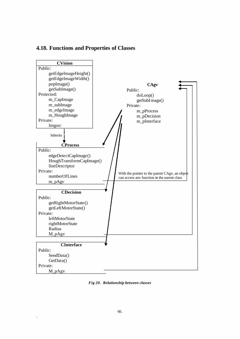
66. .
4.18. Functions and Properties of Classes
CVision
Public: getEdgeImageHeight() getEdgeImageWidth() popImage() getSubImage()
Protected: m_CapImage m_subImage m_edgeImage m_HoughImage
Private: Imgsrc
CAgv
Public: doLoop() getSubImage()
Private: m_pProcess m_pDecision m_pInterface
CProcess Public:
edgeDetectCapImage() HoughTransformCapImage() lineDescriptor
Private: numberOfLines m_pAgv
CDecision
Public: getRightMotorState() getLeftMotorState()
Private: leftMotorState rightMotorState Radius M_pAgv
CInterface
Public: SendData() GetData()
Private: M_pAgv
Inherits
With the pointer to the parent CAgv, an object can access any function in the parent class
Fig 20. Relationship between classes
67. .
A little more thought needs to be kept to the structure of the CAgv class and how
we might use objects created from it. As shown in our diagram, a real AGV
includes different stages of processes to perform its task. The information of the
image that the camera captures must be processed to detect the edges and find
out the line descriptions. Similarly, the decisions should be made and the
necessary instructions whether to move left, right, forward, backward or stop.
The data are then send to the respective motors controlling circuitry. Hence, the
image processing unit, decision unit and interface unit need to communicate with
one another so that information can be passed between the friend objects that the
AGV owns.
For this we use the CAgv object itself as the link between the object it owns. We
store the pointers to the objects that are the main components of the AGV and
then create the objects dynamically in the AGV class constructor.
This allows us to pass to the Process, Decision and Interface objects a pointer to
the parent AGV, when these objects are created. Any of the objects could then
obtain a pointer to any of the other objects through member functions of the
CAgv class. To implement this we use three member variables in the CAgv class.
o m_pProcess – a pointer to an object of class CProcess
o m_pDecision – a pointer to an object of class CDecision
o m_pInterface – a pointer to an object of class CInterface, and
o m_pAgv – a pointer to the main class CAgv.
4.18.1. CAgv
CAgv is the main class which controls other classes in this project.
The Declaration of CAgv is as:
class CAgv { public: CAgv(); virtual ~CAgv(); void doLoop(DWORD popDelay, char *szFileName, int times); //doLoop is the main control loop element.

68. .
private: CProcess* m_pProcess; CDecision* m_pDecision; CInterface* m_pInterface; friend CProcess; /* CProcess may require access to m_pInterface */ friend CDecision; /* CDecision Requires access to m_pProcess */ friend CInterface; /* CInterface Requires access to m_pDecision */ };
Now let’s consider each element of CAgv in detail:
CAgv()
A constructor CAgv() will instantiate and initialize the objects of each classes
CProcess, CDecision and CInterface. And the Destructor virtual ~CAgv() will
delete all the objects instantiated by constructor.
void doLoop(DWORD popDelay, char *szFileName, int times);
doLoop is the main control loop method which runs forever. Classes CProcess,
CDecision and CInterface are a friend of class CAgv, so all the members of these
classes can be accessed from class CAgv. Within doLoop a method to acquire
image from camera is called, an edge detection algorithm is applied on that
image, now Hough transform is applied to the image with edges to extract the
feature of an image. From the extracted feature of an image a decision is made
accordingly and finally with that decision an interface byte is sent out from
parallel port to the motor controlling circuitry.
4.18.2. CVision
This class includes the file “ViImSrc.h” (A header file of Vision SDK that deals
with the acquiring of an image from camera, manipulation of image sequence,
and other related methods that help for image processing image analysis). This
class primarily deals with the capture of image from sequence of images captured
through camera. The Declaration of CVision is:
class CVision { public: CVision(); virtual ~CVision(); void popImage(DWORD delay); void getSubImage(double percentage); int getEdgeImageWidth();

69. .
//Writes the image to a bmp file, used while coding void WriteCapImageToFile(char* szFileName); void WriteSubImageToFile(char* szFileName); void WriteEdgeImageToFile(char *szFileName); void WriteHoughImageToFile(char *szFileName); protected: CVisGrayByteImage m_capImage; CVisGrayByteImage m_subImage; CVisGrayByteImage m_edgeImage; CVisGrayByteImage m_HoughImage; private: CVisImageSource imgsrc; CVisSequence<CVisGrayBytePixel> sequence; };
Now let’s consider each element of CVision in detail:
CVision()
The CVision() constructor tries to find and connect a sequence to the image
source. And the Destructor virtual ~CVision() will try to disconnect the sequence
from the image source, if the source has been previously connected.
void popImage(DWORD delay)
Once sequence has been connected to an image source, it is ready to grab images
from the digitizer. Sequences have similar semantics to a queue. In order to get
the oldest image popImage() is called. Since by default sequences are of 0 length,
we may be forced to wait for the next available frame from the digitizer. This
waiting time is determined by the delay time passed as an argument to this
method.
void getSubImage(double percentage)
Given a percentage value as an argument, getSubImage() will reduce the image
size by percentage/2 on each side of the image.
void WritexxxxImageToFile(char* szFileName);
This method was used for debugging. Each time the captured image is
manipulated, the changed image was written to a file of type .bmp so that the
result expected was easily verified.
int getEdgeImageWidth()

70. .
For image analysis and Hough transform, the width of captured image has to be
determined which is given by this method.
4.18.3. CProcess
CProcess as the name suggests contains all the methods for processing the image,
for example the process like Edge Detection, Hough Transform are included.
This class inherits the behavior of CVision. The Declaration of CProcess is:
class CProcess : public CVision { public: CProcess(CAgv *pAgv); virtual ~CProcess(); void edgeDetectCapImage(int gradientThValue); void HoughTransformCapImage(); void setLineDescriptor(int HoughThresh); int getNumberOfLines(); struct lineDescriptor{ int theta; int r; }line[40]; private: CAgv* m_pAgv; //To access the AGV Object int numberOfLines; };
Now let’s consider each element of CProcess in detail:
CProcess(CAgv *pAgv)
A pointer to an instance of class CAgv is created with the construction of
CProcess() and is deleted with the destruction ~CProcess(). Since CProcess()
class is a friend of CAgv, all the methods are visible from CAgv.
void edgeDetectCapImage(int gradientThValue)
To detect an edges present on the captured image, this method is used which
simply uses ROBERTS EDGE DETECTION ALGORITHM. The result image
with edges only is stored in “m_edgeImage”, a protected graybyte image field of
class CVision.
void HoughTransformCapImage()

71. .
The HOUGH TRANSFORM ALGORITHM is applied on the image with edge
detected, and thus resulting with a Hough Image. This Hough image is used for
feature extraction. The result Hough image is stored in “m_HoughImage”, which
is also a protected graybyte imagefield of class CVision.
void setLineDescriptor(int HoughThresh)
After Hough Image is found out, the next step will be to describe the
characteristics of line captured by the camera. Characteristic of a set of lines can
be found out by checking the pixel value of Hough image and HoughThresh
value. All of these line descriptions are stored in an array of structure containing
two elements rvalue and thetavalue, which denotes the slope of line and its
perpendicular distance from origin.
4.18.4. CDecision
Now that after feature of image has been extracted, a decision on what to do next
has to be considered which is accomplished by it. The Declaration of CDecision
is:
class CDecision { public: CDecision(CAgv *pAgv); virtual ~CDecision(); void classifyLine(); void decideNext(); motorState getRightMotorState(); motorState getLeftMotorState(); private: CAgv* m_pAgv; //so that Decision Objects can access Agv Object typeOfLine lineType; motorState leftMotorState, rightMotorState; //motorState is an enumerated data type double radius; double theta; };
Now let’s consider each element of CDecision in detail:
CDecision(CAgv *pAgv)
A pointer to an instance of class CAgv is created with the construction of
CDecision () and is deleted with the destruction ~CDecision().

72. .
void decideNext()
After a structure lineDescriptor is filled with the characteristic of line, the
decideNext method will decide whether to move the left motor Clockwise or
Counter Clockwise, move right motor, to stop both e.t.c.
motorState getRightMotorState()
motorState getLeftMotorState()
Before decoding the output data to control circuitry, the decided motorstate
should be read. These two methods will do the same
4.18.5. CInterface
After the correct decision is made, i.e. whether to move vehicle or not, if yes then
to which direction and with what speed. All of these controls is decoded and sent
out through parallel port to the control circuit. This is what CInterface is used for.
The Declaration of CInterface is:
class CInterface { public: CInterface(CAgv *pAgv); virtual ~CInterface(); void sendData();//To LPT Port int getDataOut();//To display in console private: CAgv* m_pAgv; //so that Decision Objects can access Agv Object unsigned char dataOut; //8 bit - 0 to 255 };
Now let’s consider each element of CInterface in detail:
CInterface(CAgv *pAgv)
The data value to be sent out, i.e. “dataOut” is initialized on construction of
CInterface class.
void sendData()
After checking the result from decideNext, the appropriate data to be sent is first
encoded and then sent out to parallel port. This is the primary function of this
method.
int getDataOut()

73. .
This method is also used for debugging. To continuously monitor what data has
been sent to the parallel port, furthermore the feedback data can be verified with
the data just sent out.
4.19. Wireless Control Approach
An alternative to the Image Processing mode of operation is the wireless control
mode. In this mode the control of the vehicle is done from a remote computer.
The actual control signal can either be manual or automated at the remote end.
Vehicle movement control
x x
Remote Computer Basic Stamp II
Microcontroller
Fig 21. Wireless Control Approach Block Diagram
The control of vehicle movement is done accordingly to the transmission of data
through serial communication. The Microsoft Communication Control
(MSComm) is used to send the control data bit sequence from serial port. The
receiving unit is a circuitry consisting of a Basic Stamp II micro controller which
then decodes the signal and controls the drive motors. The platform used for the
serial communication is Microsoft Visual Basic (Windows OS).
4.19.1. MSComm Control
The MSComm control provides serial communications for the application by
allowing the transmission and reception of data through a serial port. It provides
the following two ways for handling communications:
Event-driven communications is a very powerful method for handling serial port
interactions. In many situations we want to be notified the moment an event takes
place, such as when a character arrives or a change occurs in the Carrier Detect
(CD) or Request To Send (RTS) lines. In such cases, we use the MSComm
control's OnComm event to trap and handle these communications events. The
OnComm event also detects and handles communications errors.

74. .
We can also poll for events and errors by checking the value of the CommEvent
property after each critical function of your program. This may be preferable if
the application is small and self-contained. For example, if we are writing a
simple phone dialer, it may not make sense to generate an event after receiving
every character, because the only characters we plan to receive are the OK
response from the modem.
Each MSComm control we use corresponds to one serial port. If we need to
access more than one serial port in the application, we must use more than one
MSComm control. The port address and interrupt address can be changed from
the Windows Control Panel. Although the MSComm control has many
important properties, few of them are listed below:
Properties Description CommPort Sets and returns the communications port number.
Settings Sets and returns the baud rate, parity, data bits, and stop bits as a string. PortOpen Sets and returns the state of a communications port. Also opens and closes a port. Input Returns and removes characters from the receive buffer.
Output Writes a string of characters to the transmit buffer.
Table 2. Important MSComm Control Properties
The Communications control allows us to add both simple serial port
communication functionality to the application and advanced functionality to
create a full- featured, event-driven communications tool. It also provides an
interface to a standard set of communications commands. It allows you to
establish a connection to a serial port, connect to another communication device
(a modem, for instance), issue commands, exchange data, and monitor and
respond to various events and errors that may be encountered during a serial
connection.
Possible Uses
• To dial a phone number.
• To monitor a serial port for incoming data.
• To create a full- featured terminal program.

75. .
4.19.2. Serial Port
Serial refers to data sent over a single wire, with each bit lining up in a series as
the bits are sent. This type of communication is used over the phone system
because the system provides one wire for data in one direction.
Virtually all motherboard include built- in super I/O that add one or two serial
ports to the motherboard, meaning no additional interface card is required.
Asynchronous serial interface was designed as a system-to–system
communication port. Asynchronous means that no synchronization or clocking
signal is present, so characters may be sent with any arbitrary time spacing.
Each character send over a serial connection is framed by a standard start-and-
stop signal. A single 0 bit, called the start bit, precedes each character to tell the
receiving system that the next eight bit constitute a byte of data. One or two stop
bits follow the character to signal that the character has been sent. At the
receiving end of the communication, characters are recognized by the start-and-
stop signal instead of by the timing of their arrival. The asynchronous interface is
character- oriented and has about a 20% overhead for the extra information
needed to identify each character.
Serial ports may connect to a variety of devices as modems, plotters, printers,
other computers, bar code readers, scales and device control circuits. Basically,
anything that needs a two-way connection to the PC uses the Industry-Standard
Reference Standard number 232revision C (RS-232c) serial port. This device
enables data transfer between otherwise incompatible devices.
The heart of any serial port is the Universal Asynchronous Receiver/Transmitter
(UART) chip. This chip completely controls the process of breaking the native
parallel data within the PC into serial format and later converting serial data back
into the parallel format.

76. .
9-PIN (AT) Serial Port Connector
Fig 22. 9-pin AT Serial Port Connector
Pin Signal Description I/O 1 2 3 4 5 6 7 8 9
CD RD TD DTR SG DSR RTS CTS RI
Carrier Detect Receive Data Transmit Data Data Terminal Ready Signal Ground Data Set Ready Request To Send Clear To Send Ring Indicator
In In Out Out - In Out In In
Table 3. 9-pin Serial Port Pin-Out
25-PIN (PC, XT and PS/2) Serial Port Connector
Fig 23. 25-pin Serial Port Connector
Pin Signal Description I/O 1 2 3 4 5 6 7 8 9 11 18 20 22 25
- TD RD RTS CTS DSR SG CD - - - DTR RI -
Chasis Ground Transmit Data Receive Data Request To Send Clear To Send Data Set Ready Signal Ground Carrier Detect + Transmit Current Loop Return - Transmit Current Loop Data + Receive Current Loop Data Data Terminal Ready Ring Indicator - Receive Current Loop Return
- Out In Out Out Out In Out In In
Table 4. 25-pin Serial Port Pin-Out
4.19.3. Serial Port Configuration:
Each time a character is received by a serial port, it has to get the attention of the
computer by raising an Interrupt Request line (IRQ). Eight-bit ISA bus systems

77. .
have eight of these lines and systems with 16-bit ISA bus have 16 lines. The
8259 Interrupt Controller chip usually handles their request for attention. In
standard configuration, COM1 uses IRQ4 and COM2 uses IRQ3.
When a serial port is installed in a system, it must be configured to use specific
I/O addresses (ports) and interrupts (called IRQs for Interrupt Request).
System COMX Port IRQ All All ISA Bus ISA Bus
COM1 COM2 COM3 COM4
3F8-3FFh 2F8-2FFh 3F8-3EFh 2E8-2EFh
IRQ4 IRQ3 IRQ4 IRQ3
Table 5. Standard Serial I/O Port Addresses and Interrupts
4.19.4. USER INTERFACE
Major Functions Used
Form_keydown()
According to the key pressed on form the botMove () function is called with the
corresponding movecode.
botMove()
This function is used to send the string byte through the serial port. According to
the key pressed by the user, the corresponding data byte will be transmitted.
78. .
5. Electronic Design
5.1. Introduction
The AGV had stood as an electronic challenge from its humble beginnings. This
challenge involved the design of a motor controller capable of controlling the
drive motors at variable speeds in forward and reverse directions so that the two
forward drive wheels could be driven electrically. DC motors were chosen for its
simplicity and precise control of speed. Moreover, as the power supply for the
AGV (which is mobile) is a DC battery, a DC Motor makes better sense than
using AC motors. The disadvantage of using DC motors as seen by the team is
that DC motors are not easily available in the market of the homeland of the team
members, which happens to be a third world country! Other disadvantages
include high price to power ratings.
The two front drive motors of the AGV would require independent controllers
for independent drives as required by the skid-steering principle. The principle of
DC motors and its control will be explained in the first half of this section.
The next hurdle faced was to make the AGV know about its surroundings by
means of sensors. Sensors are the major part of any intelligent robotic system.
Utilizing the limited and scarce components available the AGV team was able to
come up with CCD (Charged Coupled Device) Camera, ultrasonic and optical
emitter-detector sensors. These three sensors constitute three of the four modes
of operation of the AGV. The mode of operation can be selected by means of
jumpers. The modes are controlled by the Basic Stamp II microcontroller.
5.1.1. CCD Camera – Image Processing Mode
A powerful method for a robot to sense its environment is through robotic vision.
An USB (Universal Serial Bus) digital video camera was chosen as the source of
vision. The camera is powered from the USB port itself.
79. .
Robotic Vision would involve image processing and extensive computing power.
Thus a fast Pentium III 800MHz CPU was chosen to crunch the bits of the
captured image. The image processing program would send out information for
the motor controller boards through the parallel port. This interfacing between
the software and the hardware proved to be another challenge.
5.1.2. Ultrasonic Mode – Obstacle Avoidance
In this mode, the vehicle moves ahead straight until obstructed by an obstacle.
The presence of an obstacle is detected by the reflective property of the obstacle
to ultrasonic sound waves. Two such detectors are placed at the left and right
positions of the front side of the vehicle.
5.1.3. Emitter Detector – Line Following
The ‘G’ in the AGV means the AGV is guided by some means. One of the
easiest and intuitive way by which the AGV can be guided is by means of an
emitter detector set, made to follow a given line on the floor.
5.1.4. Manual Wireless Control Mode
This is the fourth mode in which the AGV can be operated in. Wireless control
would involve manual control of the vehicle without wires. Manual control may
not justify the true name of AGV – Autonomous Guided Vehicle, but this mode
proves to be quite interesting for the robotic enthusiast. In this mode, the
direction of travel is signaled from a remote computer using the serial port,
which is transmitted via AM waves, and received and sent to be processed by the
Basic Stamp II microcontroller.
5.2. DC Motor
DC motors are widely used in industrial and consumer applications. The speed of
the DC motor can be controlled much more easily than the AC motors. Thus the
adaptability of DC motor in speed control finds its application in modern
industrial drives.
80. .
In this project, two DC motors are used in the front wheels. The DC motors are
used to drive the vehicle. The forward and reverse drive of the two motors can
drive the vehicle in forward or backward direction or skid-steer the vehicle when
the speed of the two motors is different. The third wheel at the back is a free
castor wheel.
5.2.1. Construction of the DC Motor
Like any rotating machine DC motor also consist of a rotor and a stator.
Concentrated magnetic poles are created from field windings mounted in the
stator and the armature windings are wound in the cylindrical rotor. The armature
is distributed type and may be wound in various ways.
Depending upon the source of magnetic flux, DC motors are classified as PMDC
motors and excited DC motors. In PMDC motors, permanent magnets are
mounted in the stator with alternating poles. In excited type motors, magnetic
flux is produced by exciting the field windings wound around the salient pole.
The two ends of the armature winding is connected to two conducting segments
insulated from each other and to the shaft, to which they are mounted to.
Armature excitation is applied to the commutator segments by means of brushes.
The armature is mounted on a shaft, which is supported by the bearings. One end
of the shaft is coupled mechanically to the external load.
Some important facts to be considered in construction of DC motors
The brushes are kept electrically in the inter-polar region and hence make 900
electrical with the axes of the adjacent poles.
The brushes are alternatively positive and negative.
The number of brushes depends upon the armature winding and number of poles.
5.2.2. PMDC Motors
PMDC motors are constructed using permanent magnets made up of materials
having high residual flux and high coercivity for the field. PMDC motors have

81. .
the advantage of no field windings and no field loss and hence are smaller in
size. The PMDC motors offer the characteristics of a shunt motor and can be
controlled by armature control method.
5.2.3. Characteristics of DC motor
Fig 24. Characteristics of Shunt DC Motors (V, If constant)
The characteristics of DC motors are governed by two fundamental relation ships
i.e. emf and torque relationships.
Ea = Kaφω = φnZP/60A &
T = φIaZP/2πA = KaφIa
To study the characteristic (speed and torque characteristics), it is convenient to
express the fundamental relations in terms of speed and torque.
n = 60AEa/PZφ�= KNEa/φ &
Τ=� KTφΙa
As we know, PMDC motors show similar characteristics to that of shunt type DC
motors.
For a shunt DC motor, the induced emf in armature windings is given by
Ea = V – IaRa
which gives on substitution to above equations
n = KN(V – IaRa)/�φ

82. .
Also for PMDC motors f i.e. flux per pole is constant. From the above relation, it
is obvious that the speed may fall due to armature resistance drop slightly. Also
torque current characteristic is a fairly straight line slightly sloping downwards.
Speed torque characteristics also plays an important role in the performance of
DC motors. From the relation for and speed and torque, eliminating Ia we get,
n = KNV/φ – KNRaT/�φ2KT
which is an equation of a straight line. But due to the armature reaction, speed
falls off slightly from no load to full load, however the speed remains fairly
constant.
5.2.4. DC Motor Used
Under the limited budget and scarce availability, two identical DC wiper motors
were used to drive the AGV wheels. Though the motors were rated at a mere
17watts, at 12 volts, the motors drew a stall current of 2.5A. The vehicle had to
be engineered according to this limiting power.
Fig 25. The DC Motor used for the AGV

83. .
5.3. Speed Control of DC Motor
The speed of the DC motors is given by
n = Kn (V – IaRa)/φ
This equation shows that speed of DC motor can be controlled by two methods.
The first method is to change the flux per pole, φ, and the second method is to
change the armature voltage V. The first method is known as field control and
the second method is armature control.
However, the wiper motor we are using is a Permanent Magnet DC motor
(PMDC), so the flux per pole is always constant. So field control method cannot
be used to control speed the only alternative available is to vary the armature
voltage.
The main requirement of armature control scheme is the varying voltage supply
to the armature. This can be obtained in various ways such as use of converters,
choppers etc. As AGV has a DC Battery as a power supply, a chopper is the
viable solution for the speed control of DC Motor.
5.3.1. Chopper and PWM
A chopper is a static device that converts fixed de input voltage to a variable dc
output voltage directly. A chopper may be thought of as dc equivalent of an ac
transformer since they behave in an identical manner. As choppers involve one
stage conversion, these are more efficient. As with AGV, the future electric
automobiles are likely to use choppers for their speed control and braking.
Chopper systems offer smooth control, high efficiency, fast response and
regeneration.
The power semiconductor devices used for a chopper circuit can be power BJT,
power MOSFET, GTO or force-commutated thyristor. These devices, in general,
can be represented by a switch SW with an arrow as shown in Figure 26. When
the switch is off, no current can flow. When the switch is on, current flows in the

84. .
direction of arrow only. The power semiconductor devices have on-state voltage
drops of 0.5 V to 2.5 V across them.
Like a transformer, a chopper can be used to step down or step up the fixed dc
input voltage. We would be using a step-down dc chopper to obtain various
voltage levels below the 12V dc battery supply, which would in turn control the
speed of the motor.
A chopper is basically a high speed on/off semiconductor switch. It connects
source to load and disconnects the load from source at a fast speed. In this
manner, a chopped load voltage as shown in Figure 26(b) is obtained from a
constant dc supply of magnitude Vs.
Fig 26. An Elementary Chopper Circuit and (b) output voltage and current waveforms
In Figure 26 (a), a chopper is represented by a switch SW inside a dotted
rectangle, which may be turned-on or turned-off as desired. During the period
Ton, the chopper is on and the load voltage is equal to source voltage Vs. During
the interval Toff, the chopper is off, and the load current flows through the
freewheeling diode FD. As a result, load terminals are short circuited by FD and
load voltage is therefore zero during Toff. In this manner, a chopped dc voltage is
produced at the load terminals.
The load current as shown in Figure 26 (b) is continuous. From Figure 26 (b), the
average load voltage Vo is given by

85. .
Thus load voltage can be controlled by varying duty cycle α. The above equation
shows that load voltage is independent of load current.
Thus the average value of output voltage Vo can be controlled through α by
opening and closing the semiconductor switch periodically. The various control
strategies for varying duty cycle are as follows:
Constant Frequency System (PWM)
Variable Frequency System (PFM)
In the Constant Frequency System, the on-time Ton is varied but chopping
frequency f (or chopping period T) is kept constant. Variation of Ton means
adjustment of pulse width, thus the name Pulse Width Modulation (PWM). This
scheme has also been referred to as time-ratio control (TRC) by some authors.
Fig 27. Principle of Pulse Width Modulation (Constant T)
Figure 28 illustrates the principle of PWM. Here chopping period T is constant.
In Figure 28 (a), Ton = ¼ T so that α = 0.25 or α = 25%. In fig 28 (b), Ton = ¾ T
so that α = 0.75 or 75%. Ideally a can be varied from zero to infinity. Therefore
output voltage can be varied between zero and source voltage Vs.

86. .
Fig 28. Principle of Frequency Modulation (a) on-time Ton constant and (b) off-time Toff constant
In the Variable Frequency Scheme, the chopping frequency f (or chopping period
T) is varied and either (i) on-time Ton is kept constant or (ii) off- time Toff is kept
constant. This method of controlling α is also called frequency-modulation
scheme.
Figure 28 illustrates the principle of frequency modulation. In Figure 28 (a), Ton
is kept constant but T is varied. In the upper diagram of Figure 25 (a), Ton = ¼ T
so that α = 0.25. In the lower diagram of Figure 25 (a), Ton = ¾ T so that α =
0.75. In Figure 28 (b), Toff is kept constant and T is varied. In the upper diagram
of this figure, Ton = ¼ T so that α = 0.25 and in the lower diagram Ton = ¾ T so
that α = 0.75.
Frequency modulation scheme has some disadvantages as compared to pulse-
width modulation scheme. These are as under:
i) The chopping frequency has to be varied over a wide range for the control of
output voltage in frequency modulation. Filter design for such wide frequency
variation is, therefore, quite difficult.

87. .
ii) For the control of α, frequency variation would be wide. As such, there is a
possibility of interference with signaling and telephone lines in frequency
modulation scheme.
iii) The large off-time in frequency modulation scheme may make the load
current discontinuous which is undesirable.
It is seen from above discussions that constant frequency (PWM) scheme is
better than variable frequency scheme. PWM technique has, however, a
limitation such as, Ton cannot be reduced to near zero for most of the
commutation circuits used in choppers. As such, low range of α control is not
possible in PWM. This can, however, be achieved by increasing the chopping
period (or decreasing the chopping frequency) of the chopper.
5.4. H-Bridge
5.4.1. Theory
Fig 29. BJT H-Bridge
A circuit known as the H-bridge (named for its topological similarity to the letter
H") is commonly used to drive motors. In this circuit (depicted in Figure 29), two

88. .
of four transistors are selectively enabled to control current flow through a
motor.
As shown in Figure 30, an opposite pair of transistors (Transistor One and
Transistor Three) is enabled, allowing current to flow through the motor. The
other pair is disabled, and can be thought of as out of the circuit.
Fig 30. The H-Bridge with left to right current flow
By determining which pair of transistors is enabled, current can be made to flow
in either of the two directions through the motor. Because permanent-magnet
motors reverse their direction of turn when the current flow is reversed, this
circuit allows bidirectional control of the motor.
It should be clear that one would never want to enable Transistors One and Two
or Transistors Three and Four simultaneously. This would cause current to flow
from Power+ to Power-.
To facilitate control of the H-bridge circuit, enable circuitry as depicted in Figure
31 is typically used. In this circuit, the inverters ensure that the vertical pairs of
transistors are never enabled simultaneously. The Enable input determines
whether or not the whole circuit is operational. If this input is false, then none of
the transistors are enabled, and the motor is free to coast to a stop.

89. .
Fig 31. The H-Bridge with Enable Circuitry
By turning on the Enable input and controlling the two Direction inputs, the
motor can be made to turn in either direction.
Note that if both direction inputs are the same state (either true or false) and the
circuit is enabled, both terminals will be brought to the same voltage (Power + or
Power – respectively). This operation will actively brake the motor, due to the
back EMF property of motors, in which a motor that is turning generates a
voltage counter to its rotation. When both terminals of the motor are brought to
the same electrical potential, the back EMF causes resistance to the motor's
rotation.

90. .
5.4.2. H-Bridge Design
Fig 32. Power H-Bridge Design
The above H-Bridge is the final design for the AGV drive motors. Two such
Bridges were constructed for the two drive motors. A brief overview of its design
follows:
Transistor Selection
The first thing to consider is rating of the DC Motor. As seen on Section 5.2.4,
the DC motor had a stall current of 2.5A at 12 volts. The bridge was thus
designed for a motor current of 3A. Robust power BJTs were chosen as the
switching element after repeated destruction of the limited power MOSFETs.
Sure, MOSFETS have very less Drain to Source voltage drop, but they are very
hard to handle, as they are more static sensitive.
2N3055 NPN power BJT was chosen as the lower side switching element, and its
complementary MJ2955 PNP power BJT was chosen as the upper side switching
element due to its cheap price, good performance, and availability. These power
BJTs have a continuous collector current rating of 15A, overkill for the 2.5A stall
current DC motors.
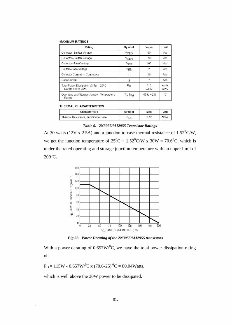
91. .
Table 6. 2N3055/MJ2955 Transistor Ratings
At 30 watts (12V x 2.5A) and a junction to case thermal resistance of 1.520C/W,
we get the junction temperature of 250C + 1.520C/W x 30W = 70.60C, which is
under the rated operating and storage junction temperature with an upper limit of
200oC.
Fig 33. Power Derating of the 2N3055/MJ2955 transistors
With a power derating of 0.657W/0C, we have the total power dissipation rating
of
PD = 115W - 0.657W/0C x (70.6-25) 0C = 80.04Watts,
which is well above the 30W power to be dissipated.

92. .
Thus no heat sink would be required. The BJTs would be directly mounted on
the PCB.
BJT Driver Design
Table 7. On Characteristics of the 2N3055/MJ2955 transistors
With a minimum DC Current Gain of 20, for a collector current of 2.5A, 125mA
base current is required to turn on the transistors. This cannot be supplied by any
of the logic circuits. Thus we need a second stage of transistors, BC547, in our
case.
Thus, when T5 is switched (CW = HIGH) on by a logic high 5V, base current is
taken off the MJ2955 PNP transistor (T1), and fed to base of the NPN 2N3055
transistor (T5). Hence T1 and T5 are turned on, driving the motor in clockwise
direction.
Similarly, when T6 is switched on (CCW = HIGH) by a logic high 5V, motor in
driven in an anticlockwise direction.
It should be noted that T5 and t6 are never to be turned on simultaneously.
5.5. Software – Hardware Interface
5.5.1. Introduction
In the Image Processing mode, the onboard computer has to ‘talk’ with the Motor
Controller boards. Each motor is assigned seven states – Stopped, 75% Full
Speed, 85% Full Speed, and 100% Full Speed in both clockwise (CW) and
counterclockwise (CCW) directions. The computer tells the Interface Circuitry

93. .
which state the motor should be run at through six motor state bits of the parallel
port.
The OS used for the image processing is Windows, a non-real-time system. The
time sharing nature of its operation may prove critical, as the vehicle may go out
of its path if the software slows down, or crashes. Thus, the interface circuits
should have fault-tolerance capabilities.
The same hardware interface should work for other modes of operation besides
the image processing mode.
5.5.2. Multiplexing
In the electronics of AGV, the commands may originate from the computer or
the Basic Stamp II. The same PWM generation and other further circuits are to
be used for both the situations – when BSII is in control and when the computer
is in control.
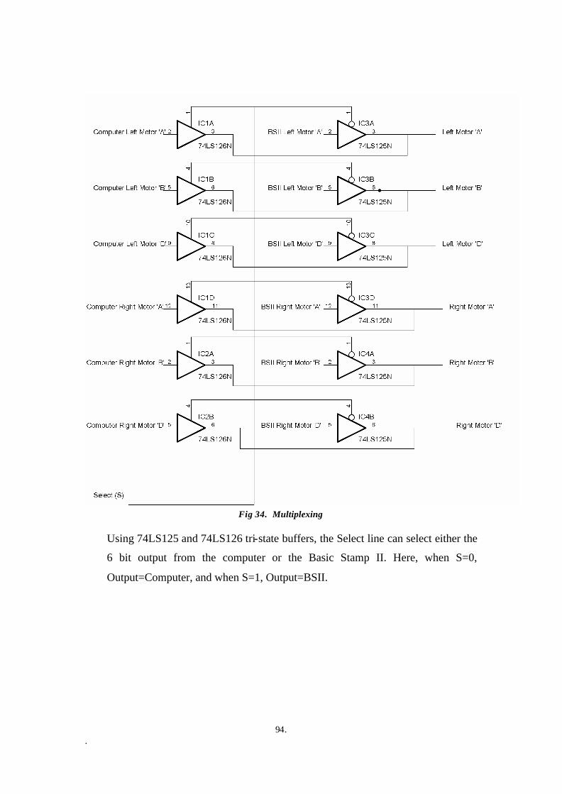
94. .
Fig 34. Multiplexing
Using 74LS125 and 74LS126 tri-state buffers, the Select line can select either the
6 bit output from the computer or the Basic Stamp II. Here, when S=0,
Output=Computer, and when S=1, Output=BSII.

95. .
5.5.3. PWM Generation
Fig 35. PWM Generator
Analyzing the astable multivibrator circuit above, we get the following results:
When A = 0 and B = 0, the reset pin of the 555 timer is held low, and the output
is low.
When A = 0 and B = 1, T2 is turned on and R2 and R6 come in parallel, and the
charging time of the 555 timer would be 0.69 (R2//R6) 27nF, and the discharging
time would be 0.69 x 1.5K x 27nF. R2 and R5 are so set that the duty cycle of the
output is around 75%.
When A=1 and B=0, T2 is turned off. Adjusting R2 we obtain a duty cycle of
around 85%.
When A=1 and B=1, T1 is turned on, and the voltage across the capacitor is held
high, so the output of the timer is a constant +5 V.
5.5.4. Direction Control
Fig 36. Direction Control
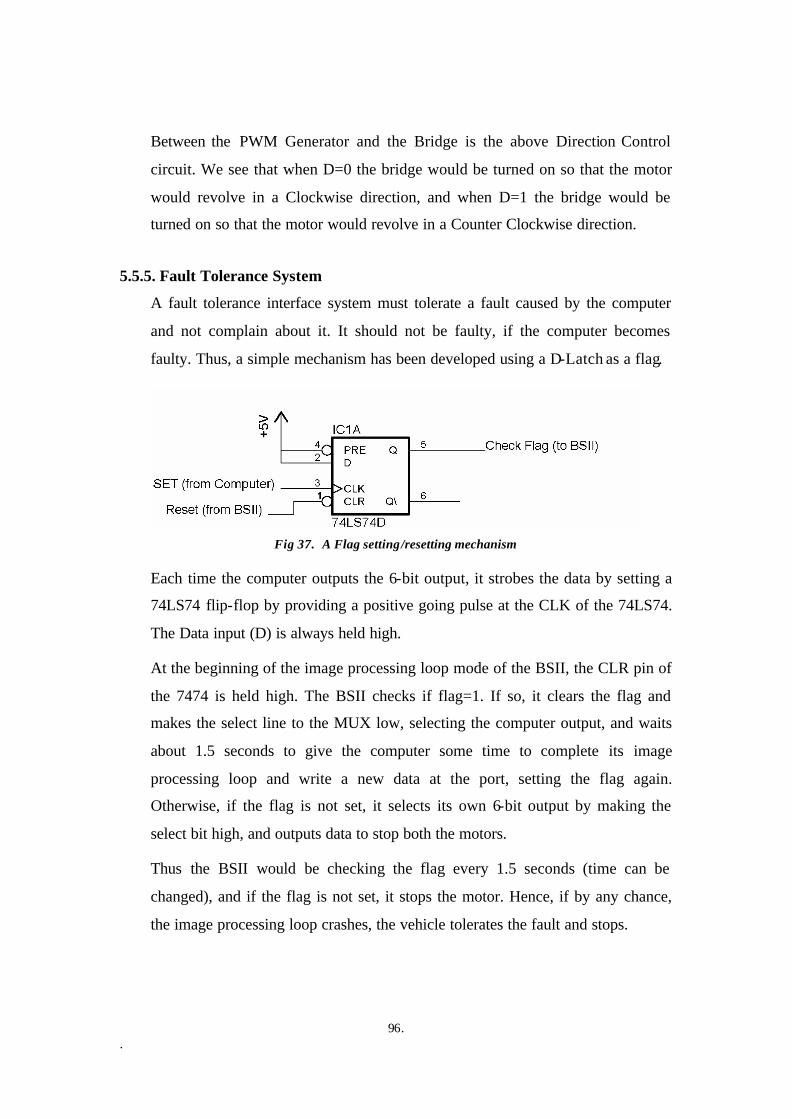
96. .
Between the PWM Generator and the Bridge is the above Direction Control
circuit. We see that when D=0 the bridge would be turned on so that the motor
would revolve in a Clockwise direction, and when D=1 the bridge would be
turned on so that the motor would revolve in a Counter Clockwise direction.
5.5.5. Fault Tolerance System
A fault tolerance interface system must tolerate a fault caused by the computer
and not complain about it. It should not be faulty, if the computer becomes
faulty. Thus, a simple mechanism has been developed using a D-Latch as a flag.
Fig 37. A Flag setting/resetting mechanism
Each time the computer outputs the 6-bit output, it strobes the data by setting a
74LS74 flip-flop by providing a positive going pulse at the CLK of the 74LS74.
The Data input (D) is always held high.
At the beginning of the image processing loop mode of the BSII, the CLR pin of
the 7474 is held high. The BSII checks if flag=1. If so, it clears the flag and
makes the select line to the MUX low, selecting the computer output, and waits
about 1.5 seconds to give the computer some time to complete its image
processing loop and write a new data at the port, setting the flag again.
Otherwise, if the flag is not set, it selects its own 6-bit output by making the
select bit high, and outputs data to stop both the motors.
Thus the BSII would be checking the flag every 1.5 seconds (time can be
changed), and if the flag is not set, it stops the motor. Hence, if by any chance,
the image processing loop crashes, the vehicle tolerates the fault and stops.
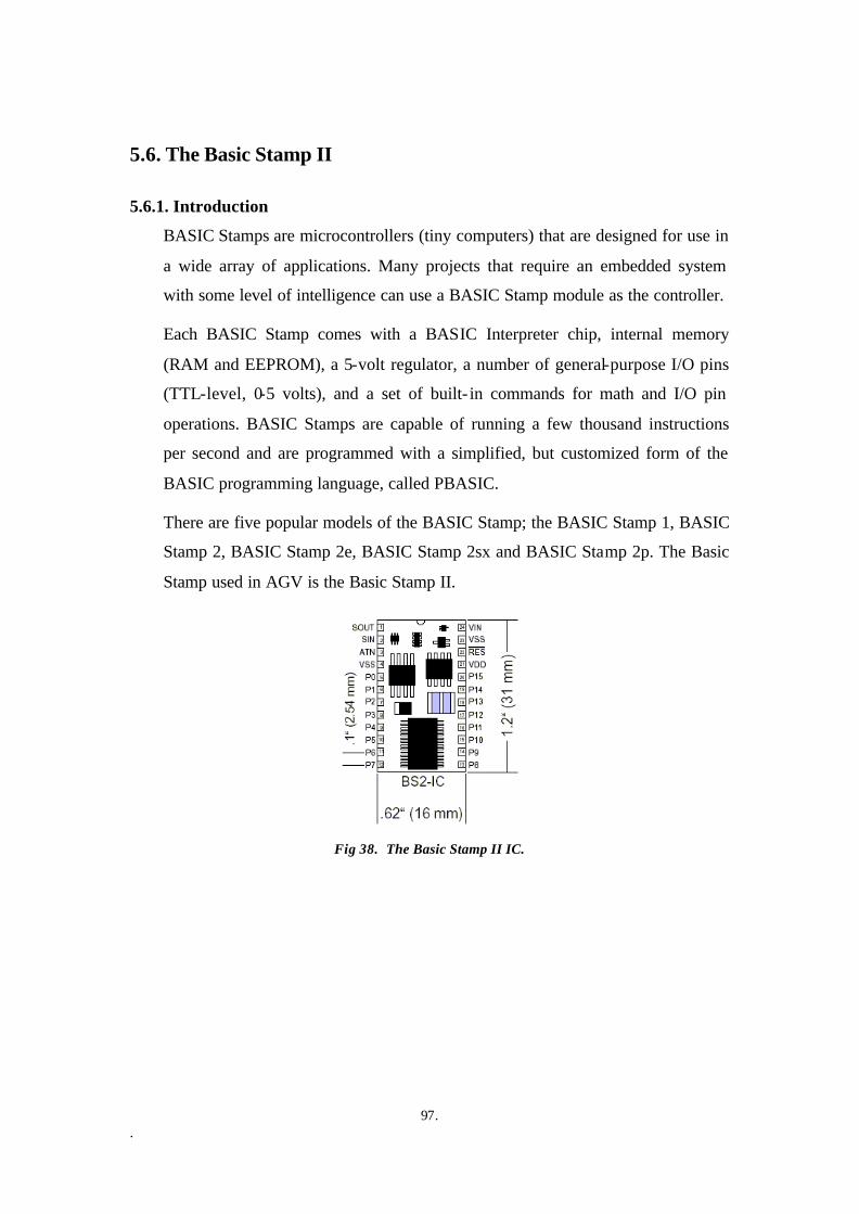
97. .
5.6. The Basic Stamp II
5.6.1. Introduction
BASIC Stamps are microcontrollers (tiny computers) that are designed for use in
a wide array of applications. Many projects that require an embedded system
with some level of intelligence can use a BASIC Stamp module as the controller.
Each BASIC Stamp comes with a BASIC Interpreter chip, internal memory
(RAM and EEPROM), a 5-volt regulator, a number of general-purpose I/O pins
(TTL-level, 0-5 volts), and a set of built- in commands for math and I/O pin
operations. BASIC Stamps are capable of running a few thousand instructions
per second and are programmed with a simplified, but customized form of the
BASIC programming language, called PBASIC.
There are five popular models of the BASIC Stamp; the BASIC Stamp 1, BASIC
Stamp 2, BASIC Stamp 2e, BASIC Stamp 2sx and BASIC Stamp 2p. The Basic
Stamp used in AGV is the Basic Stamp II.
Fig 38. The Basic Stamp II IC.

98. .
Table 8. Basic Stamp II Pin Configuration
Connecting the BSII to the Serial Port
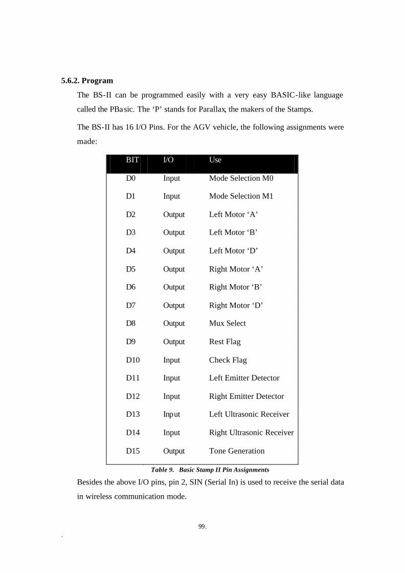
99. .
5.6.2. Program
The BS-II can be programmed easily with a very easy BASIC-like language
called the PBasic. The ‘P’ stands for Parallax, the makers of the Stamps.
The BS-II has 16 I/O Pins. For the AGV vehicle, the following assignments were
made:
BIT I/O Use
D0 Input Mode Selection M0
D1 Input Mode Selection M1
D2 Output Left Motor ‘A’
D3 Output Left Motor ‘B’
D4 Output Left Motor ‘D’
D5 Output Right Motor ‘A’
D6 Output Right Motor ‘B’
D7 Output Right Motor ‘D’
D8 Output Mux Select
D9 Output Rest Flag
D10 Input Check Flag
D11 Input Left Emitter Detector
D12 Input Right Emitter Detector
D13 Input Left Ultrasonic Receiver
D14 Input Right Ultrasonic Receiver
D15 Output Tone Generation
Table 9. Basic Stamp II Pin Assignments
Besides the above I/O pins, pin 2, SIN (Serial In) is used to receive the serial data
in wireless communication mode.

100. .
The modes can be selected by externally setting M0 and M1 according to:
M1 M0 Mode
0 0 Image Processing Mode
0 1 Emitter Detector Mode
1 0 Ultrasonic Mode
1 1 Wireless Control Mode
Table 10. Mode Selection
The program stored in the BS-II is as follows:
'{$STAMP BS2} '************************************* Pin Assignments *** '***** 'MUX Line '***** high 8 '0=Computer : 1=Basic Stamp '****** 'Mode Selection Pins 'D1 D0 = Mode ' 0 0 = Image Processing control ' 0 1 = Emitter Detector control ' 1 0 = Ultrasonic control ' 1 1 = Wireless control '****** INPUT 0 'D0 INPUT 1 'D1 '****** 'Ultrasonic sensor input '****** INPUT 14 'Left INPUT 13 'Right '***** 'Motor Outputs '***** low 2 'Left Motor A low 3 'Left Motor B low 4 'Left Motor D low 5 'Right Motor A low 6 'Right Motor B low 7 'Right Motor D '***** 'Reset pin '***** high 9 'Low to clear. Must be held high at start 'so that computer can set the flag '***** 'Flag bit for fault tolerance '***** input 10 '***** 'Emitter Detector Sensor data

101. .
'***** input 11 'Left Sensor input 12 'Right Sensor '***** 'Tone Generation - for debuggin and alarm purpose '***** output 15 'FREQ-OUT '***************************************** Main Program *** '** uC reset tone ** freqout 15, 200, 1092, 1000 pause 50 freqout 15, 200, 2092, (2092-8) pause 50 freqout 15, 200, 1092, 1000 '** Command VAR BYTE 'To store the serial data in Wireless Mode mainLoop: IF IN1 = 0 AND IN0 = 0 THEN imageProcessing IF IN1 = 0 AND IN0 = 1 THEN emitterDetector IF IN1 = 1 AND IN0 = 0 THEN ultrasonic IF IN1 = 1 AND IN0 = 1 THEN wireless '** Independent modules '****************************** imageProcessing: IF IN10 = 0 THEN flagNotSet 'Flag Set: low 8 'Mux select low - select computer. low 9 'Reset the flag high 9 'Let Computer Set Flag 'pause for 1 second and play tones at the mean time '** Image Processing One Cycle Complete tone ** freqout 15, 150, 800 freqout 15, 150, 1200 freqout 15, 150, 1000 freqout 15, 150, 1600 freqout 15, 250, 1400 '** goto mainLoop flagNotSet: high 8 'Select Basic Stamp gosub CStop 'Send data to stop goto mainLoop '****************************** emitterDetector: high 8 'Mux select high - select Basic Stamp. IF IN11 = 1 THEN lineOnLeft 'Gives greater preference to the Left Line. IF IN12 = 1 THEN lineOnRight gosub CFront goto mainLoop lineOnLeft: gosub CFrontLeft goto mainLoop lineOnRight:

102. .
gosub CFrontRight goto mainLoop '****************************** ultrasonic: high 8 'Mux select high - select Basic Stamp. IF IN14 = 0 AND IN13 = 0 THEN noObstacle IF IN14 = 0 AND IN13 = 1 THEN obstacleOnRight IF IN14 = 1 AND IN13 = 0 THEN obstacleOnLeft IF IN14 = 1 AND IN13 = 1 THEN obstacleOnLeftAndRight goto mainLoop ' Mrs. Justin Case noObstacle: gosub CFront goto mainLoop obstacleOnRight gosub CStop freqout 15, 250, 500 gosub CBack freqout 15, 500, 400 gosub CZTRRight freqout 15, 1000, 600 goto mainLoop obstacleOnLeft gosub CStop freqout 15, 250, 500 gosub CBack freqout 15, 500, 400 gosub CZTRLeft freqout 15, 1000, 600 goto mainLoop obstacleOnLeftAndRight gosub CStop freqout 15, 250, 500 gosub CBack freqout 15, 500, 400 gosub CZTRLeft freqout 15, 1000, 600 goto mainLoop '****************************** wireless: high 8 'Mux select high - select Basic Stamp. SERIN 16, 17197, [DEC Command] '1200 Baud 8 bits no parity inverted 'Once the AGV mode is changed, one more serial data must be sent 'or the interface resetted, as the program stops on this line. 'The two MSBs give the speed. D7=A D8=B 'The four LSBs give the Direction if Command = %01000001 then BackLeft01 if Command = %01000010 then Back01 if Command = %01000011 then BackRight01 if Command = %01000100 then ZTRLeft01 if Command = %01000101 then sStop01 if Command = %01000110 then ZTRRight01 if Command = %01000111 then FrontLeft01 if Command = %01001000 then Front01 if Command = %01001001 then FrontRight01 if Command = %10000001 then BackLeft10 if Command = %10000010 then Back10 if Command = %10000011 then BackRight10
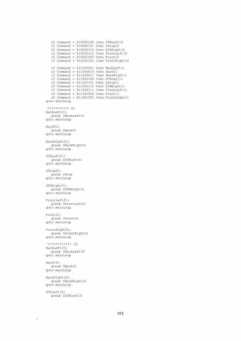
103. .
if Command = %10000100 then ZTRLeft10 if Command = %10000101 then sStop10 if Command = %10000110 then ZTRRight10 if Command = %10000111 then FrontLeft10 if Command = %10001000 then Front10 if Command = %10001001 then FrontRight10 if Command = %11000001 then BackLeft11 if Command = %11000010 then Back11 if Command = %11000011 then BackRight11 if Command = %11000100 then ZTRLeft11 if Command = %11000101 then sStop11 if Command = %11000110 then ZTRRight11 if Command = %11000111 then FrontLeft11 if Command = %11001000 then Front11 if Command = %11001001 then FrontRight11 goto mainLoop '*********** 01 BackLeft01: gosub CBackLeft01 goto mainLoop Back01: gosub CBack01 goto mainLoop BackRight01: gosub CBackRight01 goto mainLoop ZTRLeft01: gosub CZTRLeft01 goto mainLoop sStop01: gosub CStop goto mainLoop ZTRRight01: gosub CZTRRight01 goto mainLoop FrontLeft01: gosub CFrontLeft01 goto mainLoop Front01: gosub CFront01 goto mainLoop FrontRight01: gosub CFrontRight01 goto mainLoop '************ 10 BackLeft10: gosub CBackLeft10 goto mainLoop Back10: gosub CBack10 goto mainLoop BackRight10: gosub CBackRight10 goto mainLoop ZTRLeft10: gosub CZTRLeft10

104. .
goto mainLoop sStop10: gosub CStop goto mainLoop ZTRRight10: gosub CZTRRight10 goto mainLoop FrontLeft10: gosub CFrontLeft10 goto mainLoop Front10: gosub CFront10 goto mainLoop FrontRight10: gosub CFrontRight10 goto mainLoop '********** 11 BackLeft11: gosub CBackLeft goto mainLoop Back11: gosub CBack goto mainLoop BackRight11: gosub CBackRight goto mainLoop ZTRLeft11: gosub CZTRLeft goto mainLoop sStop11: gosub CStop goto mainLoop ZTRRight11: gosub CZTRRight goto mainLoop FrontLeft11: gosub CFrontLeft goto mainLoop Front11: gosub CFront goto mainLoop FrontRight11: gosub CFrontRight goto mainLoop '******************************* Common Motor Control Modules '********* 11 CBackLeft: low 2 low 3 low 4 high 5 high 6 high 7 return

105. .
CBack: high 2 high 3 low 4 high 5 high 6 high 7 return CBackRight: high 2 high 3 low 4 low 5 low 6 low 7 return CZTRLeft: high 2 high 3 low 4 high 5 high 6 low 7 return CStop: low 2 low 3 low 4 low 5 low 6 low 7 return CZTRRight: high 2 high 3 high 4 high 5 high 6 high 7 return CFrontLeft: low 2 low 3 low 4 high 5 high 6 low 7 return CFront: high 2 high 3 high 4 high 5 high 6 low 7 return CFrontRight: high 2 high 3 high 4 low 5 low 6

106. .
low 7 return '********** 01 CBackLeft01: low 2 low 3 low 4 high 5 low 6 high 7 return CBack01: high 2 low 3 low 4 high 5 low 6 high 7 return CBackRight01: high 2 low 3 low 4 low 5 low 6 low 7 return CZTRLeft01: high 2 low 3 low 4 high 5 low 6 low 7 return CZTRRight01: high 2 low 3 high 4 high 5 low 6 high 7 return CFrontLeft01: low 2 low 3 low 4 high 5 low 6 low 7 return CFront01: high 2 low 3 high 4 high 5 low 6 low 7 return CFrontRight01: high 2 low 3

107. .
high 4 low 5 low 6 low 7 return '********** 10 CBackLeft10: low 2 low 3 low 4 low 5 high 6 high 7 return CBack10: low 2 high 3 low 4 low 5 high 6 high 7 return CBackRight10: low 2 high 3 low 4 low 5 low 6 low 7 return CZTRLeft10: low 2 high 3 low 4 low 5 high 6 low 7 return CZTRRight10: low 2 high 3 high 4 low 5 high 6 high 7 return CFrontLeft10: low 2 low 3 low 4 low 5 high 6 low 7 return CFront10: low 2 high 3 high 4 low 5 high 6 low 7 return

108. .
CFrontRight10: low 2 high 3 high 4 low 5 low 6 low 7 return
5.7. Image Processing Mode
In the image processing mode, the computer grabs an image at the beginning of
the loop, processes the image, calculates and decides the states (one out of the
seven states possible) of the left and right drive motors, and sends the data out to
the parallel port at the end of the loop. It uses seven of the data bits of the parallel
port (pin 2 to pin 8)
Data Bit Command
D0 Left Motor ‘A’
D1 Left Motor ‘B’
D2 Left Motor ‘D’
D3 Right Motor ‘A’
D4 Right Motor ‘B’
D5 Right Motor ‘D’
D6 Set Flag
Table 11. Parallel Port Pin Assignments
In the above table, A, B, and D have the usual meaning as explained earlier.
5.8. Ultrasonic Mode
The AGV is made to go forward and avoid obstacles in this mode of operation. It
uses the technology of bats to locate the obstacle in front. A 40 KHz ultrasonic
transmitter receiver set is used as the sensor. The transmitter and the receiver
were kept in parallel, so that the receiver receives the tone, if an obstacle nearby
reflects the tone.

109. .
Fig 39. The Ultrasonic Transmitter Receiver Pair Arrangement
5.8.1. Ultrasonic Tone Generation
The transmitter/receiver has the best performance at 40 KHz. Even a drift a 1Khz
may prove critical for its operation. A Wien Bridge circuit is used to generate the
40KHz tone.
5.8.2. Signal Conditioning
The transducer used is an active transducer. The received signal has a 3V peak-
to-peak voltage when the ultrasonic sound is reflected from a short distance. But
the signal lacked power, i.e. the output impedance of the transducer is very high.
So an infinite gain amplifier is used to increase the signal current level. It is then
fed into a buffer in order to remove the loading effect.
Fig 40. Ultrasonic Receiver Signal Conditioning
If the amplifier stage is not to be used and the output of the transducer is to be
directly given to the buffer, the signal will die out due to the low power of the
signal, causing zero output.
A signal averager is connected to the output of the buffer. When the output of the
buffer exceeds 0.6 volts the capacitor charges instantly through the diode. Then

110. .
as the output of the buffer goes below 0.6V the capacitor discharges through the
pot (R1) set at 100K. Any other value of the resistance can be chosen for the
discharging time by varying the pot.
Then the comparator stage compares the output level of the averager circuit.
Thus, if any obstacle comes in front of the vehicle, the receiver receives the
signal and the output of the comparator is pulled low. The output of the signal
conditioning circuit is +5V when there is no obstacle, and 0V when there is an
obstacle. Two such pairs of transmitter and receiver are kept at the left and right
of the front of the vehicle. The logic levels are fed to the Stamp, and the Stamp
tries to avoid the obstacle by backing in a direction such that the obstacle is
avoided. When backing up, the tone generator circuit of the Stamp produces
three tones of 500Hz, 400Hz, and 600Hz for 250ms, 500ms, and 1s while
stopping, backing up, and turning respectively. The tones alert the user that there
is an obstacle in the path. The vehicle then tries again to go forward.
5.9. Emitter Detector Mode
In this mode, the AGV is guided along a black line in a white floor by means of
infrared Light Emitting Diodes and photodiodes. Two sets of such IR
LED/photodiode are placed at left and right of a PCB with a width of double the
line width.
Fig 41. Emitter Detector Sets.
When the vehicle is following a line (a black thick line on a white surface)
correctly, due to the arrangement, both the emitter-detector set is above the white
surface and thus the photodiode receives the IR light from the IR LED as it gets

111. .
reflected from the white surface. So the diode starts to conduct causing the output
to be equal to the supply voltage.
Now, as the vehicle starts to move away from the line, the emitter-detector set
comes above the black surface. Since the surface is black, the photodiode does
not conduct. Hence the output drops to zero.
Fig 42. Infrared Emitter Detector Arrangement
This information is fed to the Basic Stamp II, and it decides the correct way of
travel.
Note that the photodiode is placed reverse biased. If light falls on the photodiode,
the transistor T1 turns on, making the input to the BS-II E/D input pin high.
In this way, a pre-laid line is followed with the help of two emitter-detector sets.
5.10. Wireless Control Mode
In this mode of operation, a remote user can control the vehicle without any
wired link. The command for the vehicle is sent by means of asynchronous serial
communication between the computer and the Basic Stamp-II. The BSII uses the
SERIN command to recognize the serial data. (See Appendix)

112. .
5.10.1. Level Shifting
The serial data out of the RS-232C COM Port has +15V -15V voltage levels.
These voltage level is changed to an inverted TTL because the AM Transmitter
to be used needs TTL levels for its proper operation.
Fig 43. RS-232C to Inverted TTL Level Shifter
5.10.2. AM Transmission and Reception
AM Transmission and Reception were done by means of a ready-made tx/rx set
AM-RT4-418 (transmitter) and AM-HRR-418 (receiver). It has a range of 70
meters and it operated at 418 MHz. The input and output to the tx/rx is TTL
voltage level.
5.11. Power Supply
The maximum approximate power consumption of the AGV is about 180 watts.
This would include 80 watts for the on board computer and the camera, 50 watts
for each of the two drive motors. This power should be delivered by two
independent 12V 75Ah batteries, one for the two motors, and the other for the
computer and the camera. If the batteries are to be kept in parallel, the power
supply for the computer would not be regulated.
With this power arrangement, simple calculations reveal that the vehicle would
have a running period of more than eight hours with fresh batteries. After that the
vehicle should stop doing its assigned job and return back to its base station for
recharging of the batteries.

113. .
The on board Computer requires power supply either in two forms - AC power
when using the Power Supply Unit , or regulated DC voltages of different levels.
Using the Power Supply Unit assembled with the computer, we would require an
inverter (DC to AC). A Land Matic® 150 watt DC to AC Inverter is planned to
be used. The Land Matic® Inverter would also supply power to the camera's
adapter.
A more efficient design of the power supply would be not to use the Power
Supply Unit (PSU) of the computer and the AC to DC adapter of the camera.
However different levels of regulated DC voltages should be delivered. The
different DC levels for the operation of the computer are +12, -12, +5, -5, and
Ground. For the video camera, if the SONY HandyCam is to be used, it would
require 7.5V DC.
To obtain these regulated DC outputs from the 12V battery, IC Voltage
Regulators (like LM317) could be used.

114. .
6. The Product
6.1. Introduction
The Final Product of the AGV would be a programmable vehicle that could be
assigned for any job. The basic input to the vehicle would be vision to make it
autonomous. What the vehicle would do depending upon the input vision
depends on how the user would program the vehicle as.
AGVs can have uses in offices, factories, and hospitals to transport medium
weight papers, materials and stuff from one place to the other repeatedly,
avoiding obstacle, or following a line.

115. .
6.2. Gantt chart

116. .
6.3. Conclusion and Recommendation
Doing a combined project as the AGV has made mixed impressions on everyone
in the team. It has made us realize the value of team work, and to respect each
other's engineering field. Moreover, all of us have been familiarized with each
other's engineering fields.
As we are building a programmable robot, AGV is only the first stage. We would
highly recommend the continuation of this project for the coming batches using
the same base vehicle with new codes and new implementations. This would
help build a robotics community in Kathmandu University.
We hope for a successful future of the AGV.

117. .
7. Bibliography
Author’s Name (As appeared in the original reference), ” Title of the paper or
book” , Pages, Publisher, Year (and Month if a journal) of Publication.
o S.K.BOSE, A.K. HAJRA CHOUDHARY, NIRJHAR ROY; ELEMENTS
OF WORKSHOP TECHNOLOGY, VOL II; MEDIA PROMOTERS
&PUBLISHERS (PVT).LTD; 1997.
o B.S RAGHUBANSHI; A COURSE IN WORKSHOP TECHNOLOGY,
o VOL II; MANUFACTURING PROCESS; DHANPAT RAI & SONA; 1996.
o JOSEPH EDWARD SHIGLEY; MECHANICAL ENGINEERING
DESIGN,FIRST METRIC EDITION; McGRAW-HILL BOOK COMPANY;
1986
o R.K.RAJPUT; STRENGTH OF MATERIAL; S. CHAND &COMPANY;
1996
o JOSEPH HEITNER; AUTOMATIVE MECHANICS,SECOND EDITION;
EAST-WEST PRESS PRIVATE LIMITED; 1967
o C. HUTCHISON, ET.AL., “THE ARRL HANDBOOK FOR RADIO
AMATEURS 2001”, PG. 10.16, ARRL, 2001
o R. J. SCHILLING, “FUNDAMENTALS OF ROBOTICS”, CHAPTER 8,
PHI, 2000
o C. JOHNSON, “PROCESS CONTROL AND INSTRUMENTATION”,
CHAPTER 6, PHI, 2000
o HALL, ERNEST, “INTELLIGENT ROBOT TRENDS AND
PREDICTIONS FOR THE NEW MILLENNIUM”, CENTER FOR
ROBOTICS RESEARCH
o , THE 6.270 GUIDE, MIT PRESS.

118. .
o HALL, DOUGLAS V., MICROPROCESSORS AND INTERFACING,
TATA MC-GRAW HILL, 1991.
o HOROWITZ, HILL, “THE ART OF ELECTRONICS”, CHAPTER 2,
CUP, 1995
o , “BASIC STAMP MANUAL V2.0”, PARALLAX INC.
o P.H. DIETZ, “A PRAGMATIC INTRODUCTION TO THE ART OF
ELECTRICAL ENGINEERING”, 2000
o ,”ROBOTICS! STUDENT’S WORKBOOK”, PARALLAX INC.
o T. EMANUELE, V. ALESSANDRO, “INTRODUCTORY
TECHNIQUES FOR 3D COMPUTER VISION”, PH, UK
o EARL GOSE, RICHARD JOHNSONBAUGH AND STEVE JOST
(1997), PATTERN RECOGNITION AND IMAGE ANALYSIS,
PRENTICE HALL OF INDIA PRIVATE LIMITED, NEW DELHI.
o NABAJYOTI BARKAKATI (1995), OBJECT ORIENTED
PROGRAMING IN C++, PRENTICE HALL OF INDIA PRIVATE
LIMITED, NEW DELHI.
o B. CHANDRA & D.DUTTA MAJUMDER(2000), DIGITAL IMAGE
PROCESSING AND ANALYSIS, PRENTICE HALL OF INDIA
PRIVATE LIMITED, NEW DELHI.
o A K JAIN, FUNDAMENTALS OF DIGITAL IMAGE PROCESSING,
PRENTICE HALL OF INDIA PRIVATE LIMITED, NEW DELHI.

119. .
8. Appendix
8.1. Mechanical Drawings:
Fig 44. Caster Wheel
Fig 45. Caster Angle

120. .
Fig 46. FINAL DESIGN OF THE VEHICLE
Fig 47. TOP VIEW OF THE VEHICLE

121. .
Fig 48. FRONT VIEW OF THE VEHICLE
Fig 49. LEFT VIEW OF THE VEHICLE

122. .
8.2. Image Processing Code in VC++ using VisionSDK /** * Project: Autonomous Guided Vehicle * Kathmandu University, Nepal. * */ // Main.cpp: (A Console Program) // ////////////////////////////////////////////////////////////////////// #include "Agv.h" int main() { unsigned long int times=0; //Instantiate our AGV Class CAgv myAgv; //File Name to output debug BMPs char *szFile="File"; /* The Control Loop */ while(!kbhit()) //this should be infinite myAgv.doLoop(2000, szFile, times++); //the main loop is there! return 0; }

123. .
// Agv.h: interface for the CAgv class. // ////////////////////////////////////////////////////////////////////// #if !defined(AFX_AGV_H__B3AE4DC9_4AA0_44A7_8CA9_A091E1B5A26E__INCLUDED_) #define AFX_AGV_H__B3AE4DC9_4AA0_44A7_8CA9_A091E1B5A26E__INCLUDED_ #if _MSC_VER > 1000 #pragma once #endif // _MSC_VER > 1000 #include <exception>//Exception Handling #include <stdexcept>//Exception Handling #include <windows.h>//DWORD in popDelay. #include <math.h> //all the mathematics #include <conio.h> //for printer port access. /************************** Constant Definitions ***************************/ #define PI 3.1415926535 #define LPT1 0x378 /* ************************** Forward Declarations i.e. class prototypes *****************************/ class CProcess; class CDecision; class CInterface; /******************** The AGV Class *********************/ class CAgv { public: CAgv(); virtual ~CAgv(); /* doLoop is the main control loop element. */ void doLoop(DWORD popDelay, char *szFileName, unsigned long int times); private: CProcess* m_pProcess; CDecision* m_pDecision; CInterface* m_pInterface; friend CProcess; /* CProcess may require access to m_pInterface */ friend CDecision; /* CDecision Requires access to m_pProcess */ friend CInterface; /* CInterface Requires access to m_pDecision */ }; #endif // !defined(AFX_AGV_H__B3AE4DC9_4AA0_44A7_8CA9_A091E1B5A26E__INCLUDED_)
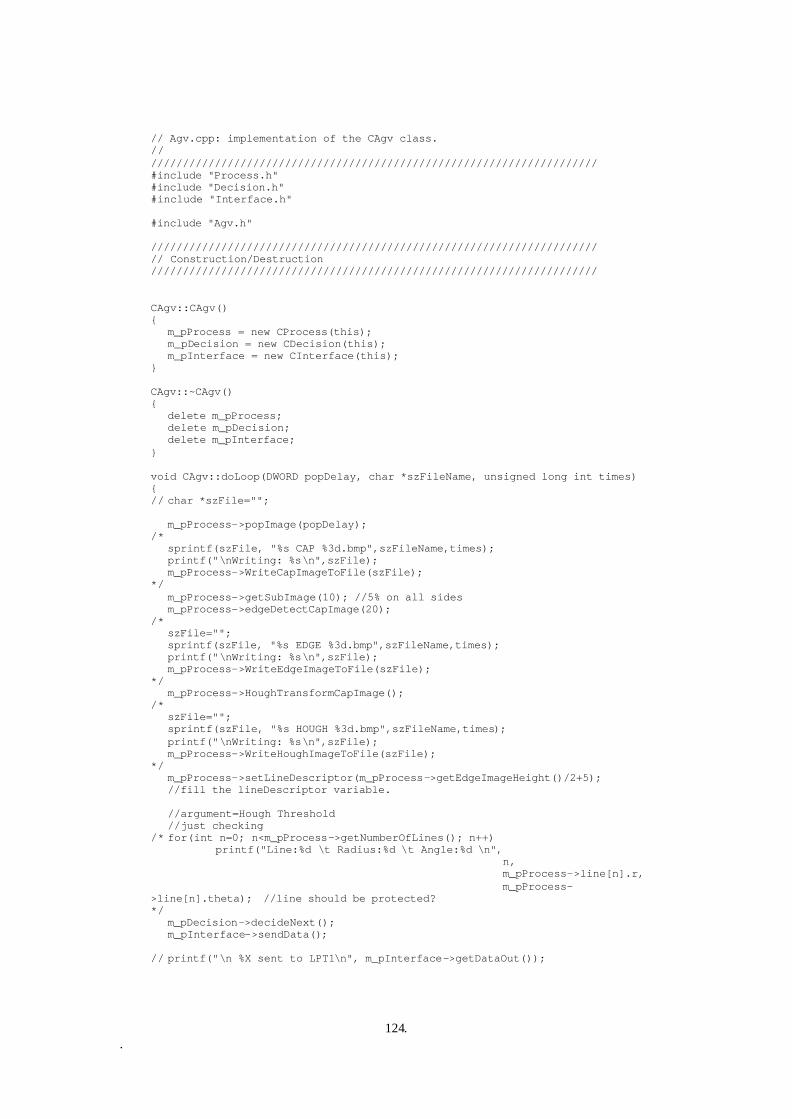
124. .
// Agv.cpp: implementation of the CAgv class. // ////////////////////////////////////////////////////////////////////// #include "Process.h" #include "Decision.h" #include "Interface.h" #include "Agv.h" ////////////////////////////////////////////////////////////////////// // Construction/Destruction ////////////////////////////////////////////////////////////////////// CAgv::CAgv() { m_pProcess = new CProcess(this); m_pDecision = new CDecision(this); m_pInterface = new CInterface(this); } CAgv::~CAgv() { delete m_pProcess; delete m_pDecision; delete m_pInterface; } void CAgv::doLoop(DWORD popDelay, char *szFileName, unsigned long int times) { // char *szFile=""; m_pProcess->popImage(popDelay); /* sprintf(szFile, "%s CAP %3d.bmp",szFileName,times); printf("\nWriting: %s\n",szFile); m_pProcess->WriteCapImageToFile(szFile); */ m_pProcess->getSubImage(10); //5% on all sides m_pProcess->edgeDetectCapImage(20); /* szFile=""; sprintf(szFile, "%s EDGE %3d.bmp",szFileName,times); printf("\nWriting: %s\n",szFile); m_pProcess->WriteEdgeImageToFile(szFile); */ m_pProcess->HoughTransformCapImage(); /* szFile=""; sprintf(szFile, "%s HOUGH %3d.bmp",szFileName,times); printf("\nWriting: %s\n",szFile); m_pProcess->WriteHoughImageToFile(szFile); */ m_pProcess->setLineDescriptor(m_pProcess->getEdgeImageHeight()/2+5); //fill the lineDescriptor variable. //argument=Hough Threshold //just checking /* for(int n=0; n<m_pProcess->getNumberOfLines(); n++) printf("Line:%d \t Radius:%d \t Angle:%d \n", n, m_pProcess->line[n].r, m_pProcess->line[n].theta); //line should be protected? */ m_pDecision->decideNext(); m_pInterface->sendData(); // printf("\n %X sent to LPT1\n", m_pInterface->getDataOut());

125. .
if (m_pInterface->getDataOut()==64) printf("\n%d. STOP\n\n", times); if (m_pInterface->getDataOut()==71) printf("\n%d. RIGHT\n\n",times); if (m_pInterface->getDataOut()==95) printf("\n%d. STRAIGHT\n\n",times); if (m_pInterface->getDataOut()==88) printf("\n%d. LEFT\n\n", times); }

126. .
// Decision.h: interface for the CDecision class. // ////////////////////////////////////////////////////////////////////// #if !defined(AFX_DECISION_H__B71845A0_FA57_4A90_86DA_9C59D475C519__INCLUDED_) #define AFX_DECISION_H__B71845A0_FA57_4A90_86DA_9C59D475C519__INCLUDED_ #if _MSC_VER > 1000 #pragma once #endif // _MSC_VER > 1000 class CAgv; //Forward Declaration enum motorState {OFF, CW, CCW}; //PWM states should be added later // for fine control /* LINE_LEFT = // // || || LINE_RIGHT = \\ \\ || || */ //enum typeOfLine {NO_LINE, SINGLE_LINE, LINE_LEFT, LINE_RIGHT}; class CDecision { public: CDecision(CAgv *pAgv); virtual ~CDecision(); // void classifyLine(); void decideNext(); motorState getRightMotorState(); motorState getLeftMotorState(); private: CAgv* m_pAgv; //so that Decision Objects can access Agv Object // typeOfLine lineType; motorState leftMotorState, rightMotorState; double radius; double theta; }; #endif // !defined(AFX_DECISION_H__B71845A0_FA57_4A90_86DA_9C59D475C519__INCLUDED_)

127. .
// Decision.cpp: implementation of the CDecision class. // ////////////////////////////////////////////////////////////////////// #include "Process.h" #include "Decision.h" #include "Interface.h" #include "Agv.h" ////////////////////////////////////////////////////////////////////// // Construction/Destruction ////////////////////////////////////////////////////////////////////// CDecision::CDecision(CAgv *pAgv):m_pAgv(pAgv) //initilazation list { leftMotorState=OFF; rightMotorState=OFF; radius=0; theta=0; } CDecision::~CDecision() { } void CDecision::decideNext() { int image_width=m_pAgv->m_pProcess->getEdgeImageWidth(); if (!m_pAgv->m_pProcess->getNumberOfLines()) { leftMotorState=OFF; rightMotorState=OFF; return; } for(int n=0; n<m_pAgv->m_pProcess->getNumberOfLines(); n++) { radius+=m_pAgv->m_pProcess->line[n].r; theta+=m_pAgv->m_pProcess->line[n].theta; } radius/=m_pAgv->m_pProcess->getNumberOfLines(); //average them theta/=m_pAgv->m_pProcess->getNumberOfLines(); if (theta>5 && theta<=90) { //Move Right leftMotorState=CCW; rightMotorState=OFF; } if (theta>90 && theta<355) { //Move Left leftMotorState=OFF; rightMotorState=CW; } if (theta<=5 || theta>=355) { if ( radius> image_width/2 + 0.15*image_width ) { //Move Right leftMotorState=CCW; rightMotorState=OFF; } else if ( radius< image_width/2 - 0.15*image_width ) { //Move Left
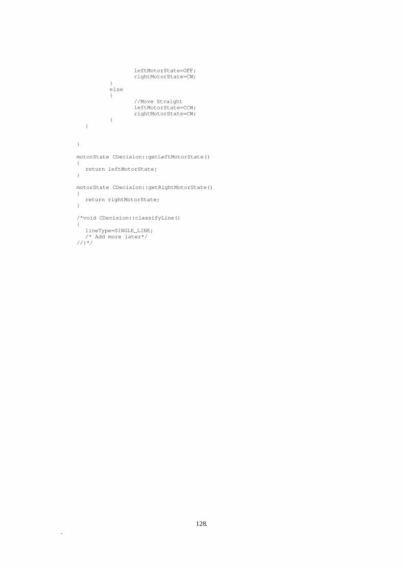
128. .
leftMotorState=OFF; rightMotorState=CW; } else { //Move Straight leftMotorState=CCW; rightMotorState=CW; } } } motorState CDecision::getLeftMotorState() { return leftMotorState; } motorState CDecision::getRightMotorState() { return rightMotorState; } /*void CDecision::classifyLine() { lineType=SINGLE_LINE; /* Add more later*/ //}*/

129. .
// Interface.h: interface for the CInterface class. // ////////////////////////////////////////////////////////////////////// #if !defined(AFX_INTERFACE_H__21A4DDF9_66FD_445C_BFB8_78CACDDCFD40__INCLUDED_) #define AFX_INTERFACE_H__21A4DDF9_66FD_445C_BFB8_78CACDDCFD40__INCLUDED_ #if _MSC_VER > 1000 #pragma once #endif // _MSC_VER > 1000 class CAgv; //Forward Declaration class CInterface { public: CInterface(CAgv *pAgv); virtual ~CInterface(); void sendData();//To LPT Port int getDataOut();//To display in console private: CAgv* m_pAgv; //so that Decision Objects can access Agv Object unsigned char dataOut; //8 bit - 0 to 255 }; #endif // !defined(AFX_INTERFACE_H__21A4DDF9_66FD_445C_BFB8_78CACDDCFD40__INCLUDED_)
130. .
// Interface.cpp: implementation of the CInterface class. // ////////////////////////////////////////////////////////////////////// #include "Process.h" #include "Decision.h" #include "Interface.h" #include "Agv.h" ////////////////////////////////////////////////////////////////////// // Construction/Destruction ////////////////////////////////////////////////////////////////////// CInterface::CInterface(CAgv *pAgv):m_pAgv(pAgv) //initilazation list { dataOut=0x00; } CInterface::~CInterface() { } /** * Assuming D2D3 is for Left motor and D1D0 is for Right Motor * 00 = stop; 01=CW; 10=CCW; 11=NEVER DO THIS. */ void CInterface::sendData() { switch(m_pAgv->m_pDecision->getLeftMotorState()){ case OFF: dataOut = 0x00; //00 xxx 000 break; case CW: dataOut = 0x03; //00 xxx 011 break; case CCW: dataOut = 0x07; //00 xxx 111 break; default: dataOut = 0x00; //00 xxx 000 break; } switch(m_pAgv->m_pDecision->getRightMotorState()){ case OFF: dataOut |= 0x00; //00 000 xxx break; case CW: dataOut |= 0x18; //000 011 xxx break; case CCW: dataOut |= 0x38; //00 111 xxx break; default: dataOut |= 0x00; //00 000 xxx break; } _outp(LPT1,dataOut); /* Clock at D6 -Positive Edge- */ dataOut |= 0x40; //01 XXX XXX // for (int delayTime=400; delayTime>5; delayTime--) // printf("S");

131. .
_outp(LPT1,dataOut); } int CInterface::getDataOut() { return (int) dataOut; }

132. .
// Vision.h: interface for the CVision class. // ////////////////////////////////////////////////////////////////////// #if !defined(AFX_VISION_H__42BC1143_4816_4E52_996A_21E9CDAC9DF2__INCLUDED_) #define AFX_VISION_H__42BC1143_4816_4E52_996A_21E9CDAC9DF2__INCLUDED_ #if _MSC_VER > 1000 #pragma once #endif // _MSC_VER > 1000 #include <windows.h> #include <VisImSrc.h> //The MS-VisionSDK Library /** CVision deals with video capture and writing images to disk. CVision is independent of CAgv */ class CVision { public: int getEdgeImageHeight(); int getEdgeImageWidth(); CVision(); virtual ~CVision(); void popImage(DWORD delay); void getSubImage(double percentage); void WriteCapImageToFile(char* szFileName); void WriteSubImageToFile(char* szFileName); void WriteEdgeImageToFile(char *szFileName); void WriteHoughImageToFile(char *szFileName); protected: CVisGrayByteImage m_capImage; CVisGrayByteImage m_subImage; CVisGrayByteImage m_edgeImage; CVisGrayByteImage m_HoughImage; private: CVisImageSource imgsrc; CVisSequence<CVisGrayBytePixel> sequence; }; #endif // !defined(AFX_VISION_H__42BC1143_4816_4E52_996A_21E9CDAC9DF2__INCLUDED_)

133. .
// Vision.cpp: implementation of the CVision class. // ////////////////////////////////////////////////////////////////////// #include "Vision.h" #include <exception> #include <stdexcept> ////////////////////////////////////////////////////////////////////// // Construction/Destruction ////////////////////////////////////////////////////////////////////// CVision::CVision() //initialization list { imgsrc = VisFindImageSource(""); if (imgsrc.IsValid()) sequence.ConnectToSource(imgsrc, true, false); else throw("Exception - CVision::CVision(CAgv p*Agv) - Image Source not Valid"); } CVision::~CVision() { sequence.DisconnectFromSource(); } void CVision::popImage(DWORD delay) { if(!sequence.Pop(m_capImage, delay)) { sequence.DisconnectFromSource(); throw("Exception - CVision::Popimage()"); } } void CVision::getSubImage(double percentage) { int wOffset=floor(percentage*m_capImage.Right()/100); int hOffset=floor(0.1*m_capImage.Bottom()); m_subImage=m_capImage.SubImage(m_capImage.Left() + wOffset/2, m_capImage.Top() + hOffset/2, m_capImage.Right()- wOffset/2, m_capImage.Bottom()-hOffset/2); m_subImage.ResetOrigin(0,0); } void CVision::WriteCapImageToFile(char *szFileName) { try{ m_capImage.FWriteFile(szFileName); } catch(exception e){ printf(e.what()); } } void CVision::WriteSubImageToFile(char *szFileName) { try{ m_subImage.FWriteFile(szFileName); } catch(exception e){ printf(e.what()); } }

134. .
void CVision::WriteEdgeImageToFile(char *szFileName) { try{ m_edgeImage.FWriteFile(szFileName); } catch(exception e){ printf(e.what()); } } void CVision::WriteHoughImageToFile(char *szFileName) { try{ m_HoughImage.FWriteFile(szFileName); } catch(exception e){ printf(e.what()); } } int CVision::getEdgeImageWidth() { return (m_edgeImage.Right()-m_edgeImage.Left()); } int CVision::getEdgeImageHeight() { return (m_edgeImage.Bottom()-m_edgeImage.Top()); }

135. .
// Process.h: interface for the CProcess class. // ////////////////////////////////////////////////////////////////////// #if !defined(AFX_PROCESS_H__CA3F39C4_BF70_42AE_867A_EBC1C308F536__INCLUDED_) #define AFX_PROCESS_H__CA3F39C4_BF70_42AE_867A_EBC1C308F536__INCLUDED_ #if _MSC_VER > 1000 #pragma once #endif // _MSC_VER > 1000 #include "Vision.h" #include "Agv.h" //class CAgv; agv.h is already included. class CProcess : public CVision { public: CProcess(CAgv *pAgv); virtual ~CProcess(); void edgeDetectCapImage(int gradientThValue); void HoughTransformCapImage(); struct lineDescriptor{ int theta; int r; }line[40]; //line whould be protected. But how to get line? void setLineDescriptor(int HoughThresh); int getNumberOfLines(); private: CAgv* m_pAgv; //To access the AGV Object int numberOfLines; }; #endif // !defined(AFX_PROCESS_H__CA3F39C4_BF70_42AE_867A_EBC1C308F536__INCLUDED_)

136. .
// Process.cpp: implementation of the CProcess class. // ////////////////////////////////////////////////////////////////////// #include "Process.h" #include "Decision.h" #include "Interface.h" ////////////////////////////////////////////////////////////////////// // Construction/Destruction ////////////////////////////////////////////////////////////////////// CProcess::CProcess(CAgv *pAgv):CVision() { m_pAgv=pAgv; } CProcess::~CProcess() { } void CProcess::edgeDetectCapImage(int gradientThValue) { double gradientX, gradientY, gradient; int j,k; /* // SOBEL int maskX[3][3]={1, 2, 1, 0, 0, 0, -1, -2, -1}; int maskY[3][3]={1, 0, -1, 2, 0, -2, 1, 0, -1}; */ // ROBERTS int maskX[2][2]={-1, -1, 1, 1}; int maskY[2][2]={-1, 1, -1, 1}; m_edgeImage=m_subImage; for(k=m_subImage.Top()+1; k<m_subImage.Bottom()-1; k++) for(j=m_subImage.Left()+1;j<m_subImage.Right()-1; j++) { /* //SOBEL gradientX= maskX[0][0]*m_subImage.Pixel(j-1,k-1) + maskX[0][1]*m_subImage.Pixel(j-1,k) + maskX[0][2]*m_subImage.Pixel(j-1,k+1) + maskX[1][0]*m_subImage.Pixel(j,k-1) + maskX[1][1]*m_subImage.Pixel(j,k) + maskX[1][2]*m_subImage.Pixel(j,k+1) + maskX[2][0]*m_subImage.Pixel(j+1,k-1) + maskX[2][1]*m_subImage.Pixel(j+1,k) + maskX[2][2]*m_subImage.Pixel(j+1,k+1) ; gradientY= maskY[0][0]*m_subImage.Pixel(j-1,k-1) + maskY[0][1]*m_subImage.Pixel(j-1,k) + maskY[0][2]*m_subImage.Pixel(j-1,k+1) + maskY[1][0]*m_subImage.Pixel(j,k-1) + maskY[1][1]*m_subImage.Pixel(j,k) + maskY[1][2]*m_subImage.Pixel(j,k+1) + maskY[2][0]*m_subImage.Pixel(j+1,k-1) + maskY[2][1]*m_subImage.Pixel(j+1,k) + maskY[2][2]*m_subImage.Pixel(j+1,k+1) ; */ //Roberts gradientX= maskX[0][0]*m_subImage.Pixel(j,k) + maskX[0][1]*m_subImage.Pixel(j,k+1) + maskX[1][0]*m_subImage.Pixel(j+1,k) + maskX[1][1]*m_subImage.Pixel(j+1,k+1); gradientY=

137. .
maskY[0][0]*m_subImage.Pixel(j,k) + maskY[0][1]*m_subImage.Pixel(j,k+1) + maskY[1][0]*m_subImage.Pixel(j+1,k) + maskY[1][1]*m_subImage.Pixel(j+1,k+1); gradient=pow(pow(gradientX/2,2)+pow(gradientY/2,2),0.5); if (gradient>gradientThValue) m_edgeImage.Pixel(j,k)=255; else m_edgeImage.Pixel(j,k)=0; } for(j=m_subImage.Left();j<m_subImage.Right(); j++) //Fill the bottom border black { m_edgeImage.Pixel(j,m_subImage.Top())=0; m_edgeImage.Pixel(j,m_subImage.Bottom()-1)=0; } for(k=m_subImage.Top();k<m_subImage.Bottom(); k++) //Fill the right border black { m_edgeImage.Pixel(m_subImage.Left(),k)=0; m_edgeImage.Pixel(m_subImage.Right()-1,k)=0; } } void CProcess::HoughTransformCapImage() { double theta_for_maxR=atan2(m_edgeImage.Bottom(),m_edgeImage.Right()); double max_HT_Rad=m_edgeImage.Right()*cos(theta_for_maxR*PI/180) + m_edgeImage.Bottom()*sin(theta_for_maxR*PI/180); CVisGrayByteImage HT(2*max_HT_Rad,360); //twice to cover the negative regions too int theta, i, j; float rad; int round_rad; for(i=m_edgeImage.Top(); i<m_edgeImage.Bottom(); i++) for(j=m_edgeImage.Left();j<m_edgeImage.Right(); j++) if(m_edgeImage.Pixel(j,i)>0) { for(theta=0;theta<360;theta++) { rad=j*cos(theta*PI/180) + i*sin(theta*PI/180); round_rad=ceil(rad)+max_HT_Rad;//position r as an index to array HT.Pixel(round_rad, theta)+=1; //increase the accumulator } } m_HoughImage=HT; } void CProcess::setLineDescriptor(int HoughThresh) { int i,j; double theta_for_maxR=atan2(m_edgeImage.Bottom(),m_edgeImage.Right());//from dr/d(theta)=0 double max_HT_Rad=m_edgeImage.Right()*cos(theta_for_maxR*PI/180) + m_edgeImage.Bottom()*sin(theta_for_maxR*PI/180); numberOfLines=0; for(i=m_HoughImage.Top(); i<m_HoughImage.Bottom(); i++) for(j=m_HoughImage.Left();j<m_HoughImage.Right(); j++) if(numberOfLines<40) if(m_HoughImage.Pixel(j,i)>=HoughThresh) if(j>=max_HT_Rad) //taking for posisitve R only, ignore the mirrors

138. .
{ line[numberOfLines].r=j - max_HT_Rad; //reposition r line[numberOfLines++].theta=i; } int temp_no_of_lines=numberOfLines; for(int k=0; k<temp_no_of_lines;k++) { } } int CProcess::getNumberOfLines() { return numberOfLines; }

139. .
8.3. Wireless Serial Communication for Remote Control Code in VB Private Sub Form_Load() If MSComm1.PortOpen = False Then MSComm1.PortOpen = True End Sub Private Sub Form_Unload(Cancel As Integer) If MSComm1.PortOpen = True Then MSComm1.PortOpen = False End Sub Private Sub Form_KeyDown(KeyCode As Integer, Shift As Integer) Select Case KeyCode 'KEYPAD (123456789)- Full Speed (11) Case 35: 'BackLeft 11 botMove (192 + 1) Case 40: 'Back 11 botMove (192 + 2) Case 34: 'BackRight 11 botMove (192 + 3) Case 37: 'ZTRLeft 11 botMove (192 + 4) Case 12: 'Stop 11 botMove (192 + 5) Case 39: 'ZTRRight 11 botMove (192 + 6) Case 36: 'FrontLeft 11 botMove (192 + 7) Case 38: 'Front 11 botMove (192 + 8) Case 33: 'Front 11 botMove (192 + 9) ',./l;'p[] - 85% Speed (10) Case 188: 'BackLeft 11 botMove (192 + 1) Case 190: 'Back 11 botMove (192 + 2) Case 191: 'BackRight 11 botMove (192 + 3) Case 76: 'ZTRLeft 11 botMove (192 + 4) Case 186: 'Stop 11 botMove (192 + 5) Case 222: 'ZTRRight 11 botMove (192 + 6) Case 80: 'FrontLeft 11 botMove (192 + 7) Case 219: 'Front 11 botMove (192 + 8) Case 221: 'Front 11 botMove (192 + 9) 'zxcasdqwe - 75% Speed (01) Case 90: 'BackLeft 11 botMove (64 + 1) Case 88: 'Back 11 botMove (64 + 2) Case 67: 'BackRight 11 botMove (64 + 3) Case 65: 'ZTRLeft 11 botMove (64 + 4) Case 83: 'Stop 11 botMove (64 + 5) Case 68: 'ZTRRight 11 botMove (64 + 6) Case 81: 'FrontLeft 11

140. .
botMove (64 + 7) Case 87: 'Front 11 botMove (64 + 8) Case 69: 'Front 11 botMove (64 + 9) End Select End Sub Private Sub botMove(moveCode As Integer) MSComm1.Output = Str(moveCode) & "!" End Sub