autonomous inertial relative navigation with sight-line
TRANSCRIPT

Autonomous Inertial Relative Navigation with Sight-Line-Stabilized Integrated Sensors for Spacecraft Rendezvous
Hari B. Hablani∗
The Boeing Company, Huntington Beach, California 92647
DOI: 10.2514/1.36559
This paper presents a novel autonomous inertial relative navigation technique with a sight-line-stabilized
integrated sensor system for midrange (20–1 km) spacecraft rendezvous. A continuous-discrete six-state extended
Kalman filter is developed for this purpose. The integrated sensor suite onboard an active chaser satellite comprises
an imaging sensor, a coboresighted laser range finder, the space-integrated Global Positioning System/inertial
navigation system, and a star tracker. For high accuracy of the relative navigation, the Kalman filter state vector
consists of the inertial position and velocity of the client satellite governed by a high-fidelity nonlinear orbital
dynamics model. The error covariance matrix is formulated in terms of the estimation error in the relative position
and velocity of the client satellite, consistent with the sensor measurements. Inertial attitude pointing and rate
commands for tracking the client satellite are determined using the estimates of the client’s inertial relative position
and velocity. To estimate the inertial attitude of the chaser satellite outside the space-integrated Global Positioning
System/inertial navigation system, anew three-axis steady-state analytical attitude estimator is developed that blends
the gyro- and the star-tracker-measured attitudes. The simulation results of amidrange spacecraft rendezvous using
glideslope guidance validate this new six-state autonomous inertial relative navigation technique. The simulation
results show that the imaging sensor’s sight line can be stabilized at the client satellite inmidrange accurately enough
to enable the laser range finder to measure the range occasionally, but these measurements are not necessary for the
midrange rendezvous phase, because the extendedKalmanfilter can estimate the rangewith the anglemeasurements
of the imaging sensor.
I. Introduction
T HE principal objective of this paper is to present a sight-line-stabilized integrated sensor system that enables novel
autonomous inertial relative navigation of a passive client spacecraftfor themidrange (20–1 km) phase of a spacecraft rendezvous. Bryan[1] explains various facets of autonomous rendezvous and docking,including its different phases and required sensors. The sensor suiteconsidered here is based on the scenario that the client spacecraft ispassive, disabled, or noncooperative, and so there is no cross-linkcommunication between the two satellites nor are there any opticalreflective geometry on the client satellite. As such, following [2,3],the selected sensor suite is an integrated sensor system composed ofan imaging sensor with wide, medium, and narrow fields of view forrelative angle measurements, a coboresighted (or collimated) laserrange finder (LRF) for range measurement, and the space-integratedGlobal Positioning System/inertial navigation system (SIGI) for theactive chaser satellite. A new autonomous relative navigationalgorithm that this sensor ensemble facilitates is formulated in aninertial frame using a continuous-discrete extended Kalman filter(EKF). To enhance accuracy of attitude estimates of the chasersatellite, the SIGI Kalman filter is provided with star trackermeasurements of the inertial attitude of the satellite. For attitudeestimation outside the SIGI, a new three-axis steady-state attitudeestimator is developed that optimally blends gyro and star trackerattitude measurements. The inertial relative position and velocityestimates of the client satellite are used to determine the pointing and
rate commands for tracking. A three-axis attitude controllerstabilizes the imaging sensor’s sight line and coboresighted LRF atthe client satellite within the pointing-accuracy requirements.Whereas the field of view of an imaging sensor is large (4 � 4 deg formedium and 1 � 1 deg for narrow fields of view), the laser beamwidth is merely �0:25 mrad (0.014 deg) and has very lowdivergence (�0:25 mrad) [3]. Therefore, whereas the pointingrequirement to avoid jitter of the imaging sensor is loose, that for theLRF is stringent (15–30 �rad). For accurate pointing, the imaging-sensor boresight and the coboresighted LRF must be aligned verycarefully [2,3]. Because achieving this degree of alignment andpointing stability is expensive, a secondary objective of this study isto show that it is not necessary to measure the range for a midrange(20–1 km) rendezvous, because it can be estimated from the anglemeasurements under certain observability conditions [4,5].
The present proof-of-concept study differs from the studies andflight tests of the past in several respects. Kawano et al. [6] illustratedthe use of relative Global Positioning System (GPS) and laser radarnavigation for the relative approach phase (from 10 km to 500m) andfinal approach phase (from 550 to 2 m) of autonomous rendezvousand docking of two engineering test satellites (ETS-VII). Thesatellites were equipped with GPS receivers and cross-link antennas.Similarly, Park et al. [7] developed a relative navigation Kalmanfilter for rendezvous of the space shuttle with the wake-shieldfacility, both vehicles having GPS receivers and the wake-shieldfacility transmitting its receiver’s output to the orbiter; the electro-optic sensors were not involved in this test. In their more recentdemonstration of theRendezvous and ProximityOperation Program,Clark et al. [8] illustrated the benefits of their relative navigationKalman filter using an LRF when the two spacecraft were within therange of a few hundred meters. Here again, because of the shortrange, the pointing accuracy of the sensors was not a concern, andrelative navigation was based on simple linear relative dynamics inthe local-vertical/local-horizontal (LVLH) frame. Gaylor andLightsey [9] emulated the SIGI Kalman filter for operation inproximity of the International Space Station, but they did not dealwith relative navigation or electro-optic sensors and their pointing.Woffinden and Geller [10] formulated relative navigation usingangles only, but their study was for very close range (25 m) in which
Presented as Paper 5355 at the AIAA Guidance, Navigation, and ControlConference and Exhibit, Austin, TX, 11–14August 2003; received 9 January2008; revision received 28May 2008; accepted for publication 29May 2008.Copyright © 2008 by The Boeing Company. All rights reserved.. Publishedby the American Institute of Aeronautics and Astronautics, Inc., withpermission. Copies of this paper may be made for personal or internal use, oncondition that the copier pay the $10.00 per-copy fee to the CopyrightClearance Center, Inc., 222 Rosewood Drive, Danvers, MA 01923; includethe code 0731-5090/09 $10.00 in correspondence with the CCC.
∗Technical Fellow, Integrated Defense Systems, Flight Sciences andAdvanced Design; currently Visiting Faculty, Department of AerospaceEngineering, Indian Institute of Technology, Kanpur 208 016, India.Associate Fellow AIAA.
JOURNAL OF GUIDANCE, CONTROL, AND DYNAMICS
Vol. 32, No. 1, January–February 2009
172

the target image nearly filled the sensor’s focal plane and estimationof the target’s relative attitudewas important for docking. To sumup,there does not appear to be a study or flight test in the past thatinvolved the sensor ensemble considered in the present study, withthe target as a point source, relative navigation in the inertial frame,Kalman filter for estimating inertial attitude of the bus using gyrosand star tracker, SIGI for inertial navigation, and glideslope guidanceof the spacecraft from a range of 20 to 1 km relative to the clientspacecraft.
The layout of this paper is as follows. Section II presents theoverall architecture of autonomous inertial relative navigation formidrange rendezvous using the integrated sensor system, acontinuous-discrete extended Kalman filter, pointing and ratecommands for tracking, a steady-state three-axis attitude estimator,and a three-axis attitude controller. Section III presents the inertialrelative navigation formulation. The relative navigation is in theinertial frame, not theLVLH frame, for the reasons explained therein.The continuous-discrete EKF is developed for the inertial relativenavigation, and nonlinear orbital dynamics are employed topropagate the inertial position and velocity estimates of the clientsatellite. Using relative position and velocity estimates of the clientsatellite, Sec. IV develops pointing and rate commands to track theclient with the integrated sensor package. Section V presents ananalytical three-axis steady-state attitude estimator to blend gyromeasurements with the star tracker measurements and produce theoptimal inertial attitude of the bus carrying the sensor package.Section VI illustrates an application of the preceding inertial relativenavigation system to a rendezvous mission in which the chasersatellite translates under glideslope guidance from an initial relativeposition of�18,�8, and 10 km to a final position of�1, 0, and 1 kmin the client satellite’s LVLH frame. SectionVII concludes the paper.
II. Overall Architecture of Autonomous InertialRelative Navigation with Integrated Sensors
Figure 1 portrays the overall closed-loop architecture of theautonomous inertial relative navigation of the client satellite with theintegrated sensor system composed of the SIGI, a star tracker, animaging sensor, and a coboresighted laser range finder. The SIGI
[11–13] provides the inertial position, velocity, attitude, and rate ofthe chaser satellite bus at 50 Hz frequency. The imaging sensorprovides the azimuth and elevation of the point-mass client satelliterelative to the sensor’s focal-plane axes at 1 Hz frequency. If theimaging sensor is pointed accurately enough (specified next), thenthe laser range finder provides the range measurement of the clientsatellite. The client satellite is a passive, disabled, noncooperativesatellite, with no GPS receiver or intersatellite communicationability, and so the differential GPS cannot be used for relativenavigation. Instead, a continuous-discrete EKF is developed for thispurpose, which uses line-of-sight angles and, possibly, the rangemeasurements. The continuous part of the navigation filter isimplemented as 50Hz propagation of the state estimate consisting ofthe client satellite’s position and velocity. Accuracy of the attitudeestimates from the SIGI is enhanced by using the star trackermeasurements [12] at 6 s intervals (1
6Hz frequency). In Fig. 1 and
later in the simulation, the SIGI star tracker attitude estimationprocess is emulated with a new three-axis steady-state attitudeKalman filter developed in Sec. V, and it provides the attitude andrate estimates for attitude control at 25 Hz.
Briefly, the closed-loop guidance, inertial relative navigation,pointing and tracking system portrayed in Fig. 1 for rendezvousoperates as follows. The target is first acquired with an imagingsensor using some acquisition methodology [3]. Whereas therequired pointing accuracy for the imaging sensor is not stringent,that for the collimated LRF is 75 �rad per axis (1�) at a 10 kmdistance. Any misalignment between the focal-plane boresight andthe LRF beam is precalibrated with precision (�20 �rad). Becausepointing accuracy of the imaging sensor is insensitive to its smallmisalignmentswith the gyros and star tracker [14], thatmisalignmentis precalibratedwith lesser precision. The 1Hz azimuth and elevationmeasurements are used along with the inertial attitude estimates ofthe bus in the inertial relative navigation Kalman filter to estimate theinertial position and velocity of the client satellite. Subtracting theinertial position and velocity estimates of the chaser satellite fromthose of the client satellite, the relative position and velocityestimates of the client satellite are obtained, which are then used tocalculate the pointing commands and rates to track the client satellite.The attitude of the chaser spacecraft is controlled and the sight line of
25 Hzθe
ωgyro
ωc
+
– 25 HzKD
+
+
Tc
25 Hz
Reactionwheel, friction,
torque limit sI1 θ
.
s1
othertwoaxes spacecraft
quaternion
q
idealtransformationto visible sensorfocal plane
Csb
visible sensor focal plane
with unknown misalignments
1 Hz
CST, b
1200– 50 Hz
SIGI gyro drift rate,random walk rate,quantization; SIGI
accelerometer measure-ments with noise; SIGI
misalignment
star tracker,its misalignment
star trackernoise
focal planeaz, el measurements
focalplanenoise
target
s1
50 Hzqgyro
1/6 Hzgyro errorcorrections
with startracker
ωgyro/ST
25 Hz
25 Hz
IKs1
pK +
qc
qgyro/ST
pointingerror
calculation
ωe
1 Hz
Kalman filterfor relativenavigationof target
LOS pointingand rate
commands
50 Hz
estimate ofrelative position and velocity of target
qc , ωc
qgyro/ST
q ST (1/6 Hz)transformation
to LVLH or inertial frame
∆V
∆V
LOS ratecommand
25 Hz
10 Hz
25 Hz
50 Hz
50 Hz
initial quaternion q (0)
Glideslopeguidance and s/c translation
dynamics
25 Hzθe
ωgyro
ωc
+
– 25 HzKD
+
+
Tc
25 Hz
reactionwheel, friction,
torque limit sI1 θ
.θ.
s1
othertwoaxes spacecraft
quaternion
q
idealtransformationto visible sensorfocal plane
Csb
visible sensor focal plane
with unknown misalignments
1 Hz
CST, b
1200– 50 Hz
SIGI gyro drift rate,random walk rate,quantization; SIGI
accelerometer measure-ments with noise; SIGI
misalignment
star tracker,its misalignment
star trackernoise
focal planeaz, el measurements
focalplanenoise
target
s1
50 Hzqgyro
1/6 Hzgyro errorcorrections
with startracker
ωgyro/ST
25 Hz
25 Hz
IKs1
pK + IKs1
pK +
qc
qgyro/ST
pointingerror
calculation
ωe
1 Hz
Kalman filterfor relativenavigationof target
Kalman filterfor relativenavigationof target
LOS pointingand rate
commands
50 Hz
estimate ofrelative position and velocity of target
qc , ωcqc , ωc
qgyro/STqgyro/ST
q ST (1/6 Hz)q ST (1/6 Hz)transformation
to LVLH or inertial frame
transformation to LVLH or
inertial frame
∆V
∆V
LOS ratecommand
25 Hz
10 Hz
25 Hz
50 Hz
50 Hz
initial quaternion q (0)
Glideslopeguidance and s/c translation
dynamics
glideslopeguidance and s/c translation
dynamics
ˆ,ˆ ˆ,ˆ
Fig. 1 SIGI imaging sensor and laser-range-finder pointing architecture for relative navigation and guidance for rendezvous (az denotes azimuth, el
denotes elevation, and s/c denotes the spacecraft.
HABLANI 173

the imaging sensor is stabilized with a proportional–integral–derivative (PID) controller and reaction wheels operating at 25 Hz[14,15]. The calculation of pointing error �e and its interesting rela-tionship with the focal-plane azimuth- and elevation-angle measure-ments (actually, their estimates) is revealed in Sec. IV. Theglideslope guidance law [16] determines the periodic �V firingsevery 60 s to bring the chaser spacecraft closer to the client spacecraftwith an exponential decrease in its relative position and relativevelocity. The �V are measured by the three orthogonal acceler-ometers of the inertial navigation system (INS), and the SIGIdetermines the inertial position and velocity of the chaser satellite at50 Hz. These are used in the continuous-discrete EKF to determinethe inertial relative position and velocity of the client satellite, as justexplained, at 50 Hz. Each of the preceding aspects of inertial relativenavigation is formulated and elaborated in the subsequent sections.
Although the LRF is coboresighted with the imaging sensor forrange measurement, [5] shows that as long as there is some relativealtitude between the two spacecraft, the in-track component of therange is observable via the in-plane angle measurements. See[4,17,18] for observability of the inertial position and velocity of thespacecraft via inertial line-of-sight angle measurements. This will beillustrated with simulation results in Sec. VI. Hence, a laser rangefinder is not essential for range measurement until the distancebetween the two satellites becomes too short (less than 1 km) to besafe without it. At such close distances, though, the client satellite’simage fills the focal plane of the sensor, and the pointingrequirements for both the imaging sensor and the LRF becomerelatively loose and the attitude control becomes relative easy.
III. Six-State Relative Navigation of the Client Satellitein the Inertial Frame
Our objective now is to develop a six-state continuous-discreteextended Kalman filter to estimate the inertial position and velocityof the client satellite relative to the chaser satellite. The formulation isin the inertial frame, not the LVLH, for three reasons. First, a largerelative in-track distance of 20 km between the two spacecraft at analtitude of 500 km is equal to an orbital arc of �3 mrad, which ismuch larger than the imaging-sensor noise 0.07mrad (1�) for a pointtarget, and therefore a 3 mrad arc cannot be treated as a nominalhorizontal boresight of the imaging-sensor focal plane, and evenmore so for the pencil laser beam. Second, at a 10 km relative range,[19] shows that the linearization of even the spherical differentialgravity between the two vehicles causes significant navigationerrors. To illustrate the errors for low-altitude 100 min orbits,consider a two-pulse rendezvous scenario in Fig. 2, in which a chasersatellite is �18 km behind and 10 km below a client satellite at a500 kmaltitude, and startingwith a guidance pulse at t� 0, it reaches1 km behind the client satellite at the same altitude in 1800 s. In theEarth’s spherical gravitation field (J2 � 0), the linearization of the
differential gravity �g �r0; r1� [see Eqs. (13) and (14)] introduces a e�gestimation error, the three components of which are shown in Fig. 3.
We observe that ke�gk is�0:1 mm=s2 at t� 0 and it approaches zero
as the chaser approaches the client satellite. But even this minute e�gerror develops a relative position estimation error greater than 100min 1800 s, as shown inFig. 4 in the client satellite’s LVLH frame. Thiserror is open-loop in that it is in the absence of measurements and arecursive estimation process; nevertheless, it suggests theinadequacy of the linearized relative dynamics model. Con-sequently, our use of this linearization for long distances in [16], inretrospect, is an error.
The third reason is concerned with the Earth’s nonsphericalgravity. The error in Fig. 4 would be aggravated if the orbitaldynamics model ignores the most predominant J2 gravitationalacceleration, which causes regression of the orbital ascending nodeand perturbs the satellite’s nominal position at twice the orbitalfrequency. For example, for a 500 km altitude orbit with 46 deginclination, the average ascending-node regression rate is 1 �rad=s.In 1800 s (a typical duration to decrease the in-track distance from 20to 1 km), the ascending node regresses by �12 km on the average.
The attendant exact perturbations in the spacecraft position from theideal circular orbit would depend on its initial location in the orbit,but the 12 km average nodal regression while the relative in-trackdistance decreases from 20 to 1 km is clearly too significant to ignoreand to use the LVLH frame for relative navigation. (We have notdetermined the relative position estimation error with J2, similar tothe error in Fig. 4, however.)
For these reasons, we use a geocentric inertial frame and a gravitymodel that includes the J2 term to propagate the orbits of bothvehicles. The higher-order gravitational accelerations are ignored inthis study.
Some features of the continuous-discrete EKF for inertial relativenavigation of the client satellite presented here are different from its
Fig. 2 Trajectory of a chaser satellite with one initial pulse and its
estimate relative to the client satellite LVLH frame.
Fig. 3 Differential gravitational acceleration estimation error due to
linearization.
Fig. 4 Relative position estimation error due to linearization of the
spherical gravity field.
174 HABLANI

textbook counterpart [20]. The azimuth and elevation angles arerelated to the relative position of the client satellite. In the EKFpresented here, this relative position is obtained by differencing theinertial positions of the two satellites, as stated earlier. Whereas thechaser satellite’s inertial position estimate is provided by the SIGI,the inertial position of the client satellite is estimated by the filter.Thus, the system dynamics model in the filter consists of the orbitaldynamics of the client satellite, and the state vector is 6 � 1. Incontrast, the state vector of the standard EKF would involve orbitaldynamics of both satellites, and the state vector would be 12 � 1 as in[4]. Further, because the measurements are related to the relativeposition of the client satellite, the linearized measurement matrixH,the transition matrix �, and the error covariance matrix P are allrelated to the relative position vector, not to the inertial position. Thesalient features of the present continuous-discrete EKF aresummarized next.
A. Six-State Inertial Relative Navigation Formulation
Figure 5 shows a client satellite and a chaser satellite in twoneighboring circular orbits. The radial vectors r1 and r0 from theEarth’s mass center denote inertial positions of the chaser and theclient satellite, respectively, governed by the following equations inthe geocentric inertial frame:
�r 1 � g�r1� � a1 (1)
�r 0 � g�r0� (2)
where g is the total (spherical plus nonspherical) Earth’s
gravitational acceleration, and a1 is the acceleration of the chasersatellite caused by the thrusters for guidance. The estimate r0 of theclient’s position in the inertial frame is governed by a similarequation:
�r 0 � g�r0� (3)
This equation, rewritten in its first-order formwith the state vector
as �r0; _r0, is used in the continuous-discrete EKF for the clientsatellite’s state estimate propagation at 50 Hz. On the other hand, theestimates of the chaser satellite’s inertial position and velocity, r1 and
_r1, are furnished by its SIGI, as stated earlier. An estimate of theposition and velocity of the client satellite relative to the chasersatellite is then
‘� r0 � r1 (4)
_‘� _r0 � _r1 (5)
where ‘ stands for the line-of-sight vector of the imaging sensormounted on the chaser satellite bus. The associated estimation errors
in terms of the estimation errors in r1, r0, _r1, and _r0 are
~‘� ~r0 � ~r1 (6)
~_‘� ~_r0 � ~_r1 (7)
where the chaser navigation estimation errors ~r1 and ~_r1 are the SIGInavigation errors.
Because the imaging sensor of the chaser satellite measuresazimuth and elevation angles of the client satellite at 1 Hz frequency(the angles illustrated in Fig. 6 and explained in Sec. IV), and becausethese measurements depend on the relative position vector ‘, not r1and r0 individually, it is convenient to perform the measurement
updates of the relative vectors ‘ and _‘. TheKalman gainK is requiredfor this update, and its evaluation, in turn, requires the measurementsensitivity matrix H and the error covariance matrix P. H will beformulated subsequently [Eq. (23)]. The 6 � 6 error covariance
matrixP for the relative position and velocity estimation errors ~‘ and~_‘ is defined as
P� E~‘~_‘
� �� ~‘ ~_‘
� �(8)
and propagated at 50 Hz as follows:
P i��� ��Pi�1����T �Q (9)
where E�� is the expectation operator, � is the 6 � 6 transitionmatrix, and Q is the 6 � 6 process noise matrix. The discrete
propagation of P at 50 Hz is our replacement of the continuouspropagation ofP in the standard continuous-discrete EKF algorithm.
Markley [21] developed an easily computable 6 � 6 Cartesianstate transition matrix� as a function of the gradient matrixG of thegravitational acceleration, evaluated both at the beginning and at theend of the propagation interval (20 ms, presently). Because the
sensor measurements are used to update ‘ (and _‘) and the line-of-sight vector ‘ originates from the chaser sensor at the inertial positionr1, the transition matrix � is evaluated at the estimates r1�ti�1� andr1�ti� provided by the SIGI. Clearly, the navigation errors of the SIGIinfluence the� and henceP. The process noisematrixQ, formulated
subsequently, accounts for these and other modeling errors. The6 � 6 transition matrix � is given by [21]
1r~
0r
0r~
ˆ
1r
EstimatedPosition of
EstimatedPosition of
Chaser
Client
Client
Chaser
1r~
0r
0r~
ˆ
1r
Fig. 5 True and estimated inertial positions of the chaser and thetarget, true and estimated relative positions of the target, and inertial
position estimation errors of the chaser and the target.
ys
ys
ε
z s
zs α
x s
ys
zs
α
αu
s
sxy=α
b
x s
x s
ys
εu
s
sxz−=ε
b
zs
ε
ys
ys
ε
z s
zs α
x s
ys
zs
α
αu
s
sxy
tan
tan
Image
Image
=αb
x s
x s
ys
εu
s
sxz−=ε
Client satellite
Client satellite
Sensor focal plane
Target image
b
zs
ε
Fig. 6 Two-axis pointing angle commands to align the focal-plane
boresight with the line of sight to the client satellite.
HABLANI 175

����r1�ti�; r1�ti�1�� ��rr �rv
�vr �vv
� �(10)
where ti�1 and ti are, respectively, the beginning and the end of thecurrent 50 Hz sample period, and
� rr � I � �2Gi�1 �Gi���t�2=6 (11a)
� rv � I�t� �Gi�1 �Gi���t�3=12 (11b)
� vr � �Gi�1 �Gi��t=2 (11c)
� vv � I � �Gi�1 � 2Gi���t�2=6 (11d)
where I is a 3 � 3 identity matrix, and Gi�1 and Gi are the gravitygradient matrices evaluated at ti�1 and ti respectively. Markley [21]furnishes the 3 � 3 gradient matrixG up to the J2 gravitational term,and to conserve space, it will not be reproduced here. Montenbruckand Gill [22] provide the gradient matrix of a much higher order forhigh-fidelity simulations, though that will not be used in this study.
Digressing for a moment, note that if the change in the gradientmatrix from r1�ti�1� to r1�ti� is ignored (that is, supposeGi�1 �Gi)and, further, if the second- and higher-order terms in�t are ignoredas well in submatrices (11), then the transition matrix� simplifies to
�� I I�tGi�t I
� �� I6�6 �
0 IGi 0
� ��t� I6�6 � A�t (12)
where I6�6 is a 6 � 6 identity matrix, and the definition of the 6 � 6matrix A is apparent. The A is indeed the state-space matrix thatgoverns the linearized dynamics of the 6 � 1 relative state vector
�‘; _‘. The second-order version of this approximate linear state-space equation of the relative motion is
�‘�G�r1�‘ � a1 (13)
where a1 is the estimate of the thruster acceleration a1. The exactnonlinear counterpart of Eq. (13) is obtained from the estimationversion of Eqs. (1) and (2):
�‘� g�r0� � g�r1� � a1 (14a)
� �g�r0; r1� � a1 (14b)
where �g�r0; r1� is the estimated differential gravity. When
linearized, �g�r0; r1� �G�r1�‘, as seen in Eq. (13). The estimation
error e�g, illustrated earlier in Fig. 3, is the difference between the
exact �g�r0; r1� and its linear approximationG�r1�‘ for the sphericalgravitational field (J2 and higher-order terms being zero).Equation (14a) also reveals why this equation is not used directlyin the EKF and Eq. (3) is used instead: solving Eq. (14a) requires apriori knowledge of the inertial positions r0 and r1, which comesfrom the integration of Eq. (3) and the SIGI, respectively, but thatrenders Eq. (14a) superfluous.
Returning to the state estimate updates at the time of sensormeasurements, the updates of the Kalman gain matrix and the errorcovariance matrix P take place at 1 Hz, and the relative position and
velocity vector estimates are updated from ‘��� to ‘��� and _‘��� to_‘���, respectively. Knowing the concurrent inertial position andvelocity estimates of the chaser satellite provided by the SIGI, theinertial position and velocity estimates of the client satellite areupdated as follows:
r 0��� � ‘��� � r1 (15a)
_r 0��� � _‘��� � _r1 (15b)
The recursive nonlinear propagation of these estimates thencontinues with the integration of Eq. (3). It is also clear from thepreceding formulation that the SIGI navigation errors infiltrate theclient satellite’s position and velocity estimation process.
B. SIGI Navigation Errors of the Chaser Satellite: A Simple Model
A detailed accurate model of the SIGI navigation errors is notavailable in public domain. Zubkow [12], for example, simply statesthat the blended GPS/INS performance of the SIGI system in theprecise positioning service mode is 16 m spherical error probabilityin position and 0:1 m=s in velocity and does not offer any model.More details on the GPS errors can be gleaned from [22,23]. Theseerrors are partly due to the gyros and accelerometers and partly due tothe GPS system, both filtered by the SIGI’s internal tightly coupledhigh-fidelity navigation Kalman filter. Misra and Enge [23] describethe GPS navigation errors as consisting of biases and zero-meannoises. The biases are due to the satellite clock errors, ephemeriserrors (3 m rms), and atmospheric propagation modeling errors (5 mrms), changing slowly as theGPS satellites’ elevation angles change;the zero-mean noises, on the other hand, are due to the receiver noiseand multipath of GPS signals (1 m rms). The combined user rangeerror is �6 m rms [23]. In this work, our intent is not to develop ahigh-fidelity model of the preceding error sources. Instead, we willrepresent the SIGI navigation errors simply with an aggregate modelas follows.
The position errors along the local-horizontal x and y axes are eachmodeled as a first-order exponentially correlated Markov process,following [24]. For example, the error along the x axis is
xe �Hdop�bx � �x� (16)
where bx is a bias error, �x is a random error, and the horizontaldilution of precision Hdop � 1:2 [17,25]; bx and �x are each first-order exponentially correlated Markov processes. For example, thediscrete version of the bias bx;i is governed by
bx;i � bx;i�1 exp���b�t� � wb;i�1 (17)
where 1=�b is the time constant of the process, �t is the sampleperiod (20ms, presently), andwb;i is the discrete white noise processwith variance equal to qb�t; qb is the power spectral density of thecontinuous white noise of which wb;i is the discrete version, andqb � 2�2b�b, with �
2b being the variance of the bias bx. Presently,
these parameters are taken as �b � 5:1 m, and 1=�b is one-eighth ofthe orbit period. The exponentially correlated random error �x ismodeled similarly, with the variance of the discrete white noise thatgenerates it equal to q��t, q� � 2�2���, �
2� � �1:4 m�2, and
1=�� � 60 s. The vertical position error ze is modeled likewise:
ze � Vdop�bz � �z� (18)
where bz and �z are defined as bx and �x are, respectively, with thesame numerical parameters; the vertical dilution of precisionVdop � 1:4.
The velocity of the satellite is measured by the Doppler shift of theGPS signal frequency. Misra and Enge [23] show that the velocityerror could be modeled as a discrete white noise sequence in eachaxis, with its standard deviation �v equal to 0:03 m=s in each axis.
Because the SIGI navigation errors contribute directly to the errorsin propagation of the relative position and velocity, the precedingmodel of the SIGI navigation errors is used to develop acorresponding process noise matrix Q. The 3 � 3 process noise
matrix Qpos
corresponding to the position error in the local-vertical/
local-horizontal frame is
Q pos � qscalar � diag�qb � qn��t�H2dop;H
2dop;V
2dop (19)
where qscalar is introduced to tune the filter. The 3 � 3 velocityprocess noise matrixQ
vel� qscalar � �2vI (I � 3 � 3 identity matrix).
176 HABLANI

C. Focal Plane Angles and Range Measurements
Figures 5 and 6 illustrate relative geometry of the two satellites, thefocal plane of the imaging sensor, and the image of the client satelliteon the focal plane. Because of imperfect tracking, the client image isat some nonzero azimuth and elevation angles relative to the focal-plane center. Let the line-of-sight (LOS) vector ‘, expressed in thesensor frameFs, have the components ‘FS � �xS; yS; zS. The LOSangle measurements at 1 Hz are thus related to the components of‘: Azimuth:
�m � �� �� � tan�1�ys; xs� � �� (20a)
Elevation:
"m � "� �" � tan�1��zs; xs� � �" (20b)
These angles aremuch less than 1 rad for the target image to bewithinthe sensor track box. The quantities �� and �" are the zero-meanrandom white noises corrupting the measurements, and theirstandard deviations would increase as the distance between the twosatellites decreases. Using these measurements and the pointingcontrol system shown in Fig. 1, the integrated sensors may besufficiently accurately pointed at the client satellite so that thecollimated laser beam would impinge upon the client and determineits relative range. The required pointing accuracy is about10–100 �rad (1�) [3,26], depending on the relative range. The noisyrange measurement is modeled as
rm � k‘k � �r (21)
where �r is a zero-mean white noise. For updates of the line-of-sight
vector estimates and its rate from ‘��� and _‘��� to ‘��� and _‘���with the preceding measurements, the usual 3 � 1 partial derivativevectors @�=@‘, @"=@‘, and @‘=@‘ are thus derived in the sensor frameand transformed to the inertial frame [24,27]:
@�
@‘FI � CIs
@�
@‘(22a)
@"
@‘FI � CIs
@"
@‘(22b)
@‘
@‘FI � CIs
@‘
@‘(22c)
where CIs � CIbCbs is the transformation matrix from the sensorframe Fs to the inertial frame FI , CIb is the transpose of the inertialattitude CbI of the spacecraft provided by the SIGI, and Cbs is thetransformation matrix from the ideal sensor frame Fs to the chaserbus frame Fb. Clearly, the gyro and star tracker errors filteredthrough the SIGI Kalman filter will influence the inertial relativenavigation Kalman filter performance. The linearized (3 � 6)measurement matrix H associated with the measurement vectorz� ��m "m rmT for updates of the Kalman gain matrix and the errorcovariance matrix is
H�
�@�
@‘FI
�T
�@"
@‘FI
�T
03�3�@‘
@‘FI
�T
26666664
37777775
(23)
where 03�3 is a 3 � 3 null matrix. Because the slopes on the right side
of Eq. (23) are computed with the estimated ‘ and the inertial attitudeestimate CIb of the chaser satellite, the SIGI navigation errorsinfluence the H matrix and thereby the estimation accuracy of thenavigation Kalman filter.
IV. Pointing Commands
A. Quaternion Commands
Figure 7 shows a client satellite and a chaser satellite in twoneighboring circular orbits. The local-vertical/local-horizontal frameat the client satellite mass center is denoted asF0, and the one at thechaser satellitemass center is denoted asF1. The pointing commandsare the attitude commands for the chaser satellite to orient itsimaging-sensor boresight to the client satellite. The sensor may besomewhat misaligned from its ideal orientation relative to the chasersatellite’s optic bench. Thesemisalignment angles are small (perhapsless than a milliradian) and unknown and not of any particularconcern in this paper. Nevertheless, letFs andF
0s be the ideal and the
misaligned frames of the sensor, respectively, and letCss0 transform avector in theF0s to the frameFs. In the misaligned frameF0s: x
0sy0sz0s,
the boresight of the sensor is along the x0S axis and the objective is topoint the boresight at the client satellite. Let b be a unit vector alongthe boresight axis. Then, in the frame F0s, b
F0s � �1; 0; 0. This unitvector is transformed to the chaser body frame Fb via thetransformation matrix Css0 and the transformation matrix Cbs; thus,bFb � Cbs Css0 bF
0s . On the other hand, the relative vector r10 from
the chaser center of mass to the client center of mass, expressed in an
inertial frameFI , is given by rFI10 ��r
FI1 � r
FI0 , where r1 and r0 are
both expressed in the frame FI. The imaging sensor is located at anoffset vector roff from the chaser center of mass (Fig. 7). Hence, theline-of-sight vector from the focal-plane center of the chaser to theclient satellite is given by ‘� r10 � CIbroff . A unit vector u alongthis line-of-sight vector is given by uFI � ‘=k‘k. The offset vectorroff is not accounted for in Sec. III, in which ‘� r10. This isacceptable at long ranges, but as the range decreases, neglecting roffintroduces a bias error in the command angles and therefore it is
considered now. Knowing the estimate ‘ from the inertial relativenavigation filter of Sec. III, the unit vector uFI can be calculated nowin the inertial frame.
Assuming that the boresight unit vector bFb is initially alignedwith the xI axis of the inertial frame, the quaternion command qcI toalign bFb with uFI is given by [28,29]
qcI �1�������������������������
2�1� b u�p
���b � u� cos�
2� �b� u� sin�
2; �1� b u� cos�
2
�(24)
where the subscript cI implies from the inertial frame to thecommanded chaser body frame; the vector part of the quaternion iswritten first and then the scalar; and � is a roll angle about theboresight or the LOS vector, used to orient the solar arrays of thesatellite normal to the sun. The angle � is not relevant in this paper;therefore, for �� 0, qcI simplifies to
Fig. 7 Relative geometry of the two satellites and the imaging-sensor
focal plane.
HABLANI 177

qcI � �b � u; 1� b u=�������������������������2�1� b u�
p(25)
If the inertial frame in Eq. (25) is replaced with the sensor frameFs, the quaternion command qcs then can be related with the smallazimuth and elevation angles on the focal plane shown earlier inFig. 6. The boresight (and laser beam) unit vector b in the sensorcoordinate frame is b� �1; 0; 0, and the LOS unit vector u in thesame frame is u� �xs=r; ys=r; zs=r, where xs, ys, and zs are thecoordinates of the client satellite relative to the chaser satellite in itssensor frame. Applying Eq. (25), the quaternion command to alignthe sensor boresight axis and the laser beam with the line-of-sightvector ‘ is found to be
qcs ��0; � zs=r; ys=r
1� xs=r
� �� �������������������������2�1� xs=r�
p(26)
Linearizing the definitions of the azimuth and elevation angles inEq. (20) for small angles, the quaternion command (26) can beapproximated as qcs � ��0; "=2; �=2; 1�, where xs � r andj�ys; zs�j � xs. The focal-plane sensor measures these angles at1 Hz frequency, as modeled in Eqs. (20). These 1 Hz measurementsare processed along with the 50 Hz gyro measurements and every 6 sstar tracker measurements by the inertial relative navigation EKF to
produce the line-of-sight vector estimate ‘ and the velocity estimate _‘at 50 Hz in the inertial frame. These estimates are then used inEq. (25) to obtain the inertial quaternion commands (and ratecommands, derived next) at 10 Hz (Fig. 1) and to generate the focal-plane angle estimates " and � at 25Hz. These estimates are the y and zcomponents of the 25 Hz attitude error signal �e in Fig. 1 for the PIDattitude controller. Note that the 1 Hz noisy focal-planemeasurements themselves are not enough to point the sensor withthe required accuracy at the client satellite.
B. Angular-Rate Commands
To stabilize the imaging sensor on the client satellite, the ratecommand !cI is required, which is related to the inertial velocity of
the LOS vector _‘, which, in the chaser body frame Fb, is
_‘ Fb � CbI� _rFI
0 � _rFI1 � � !bI � rFboff (27)
and!bI is the inertial angular velocity of the chaser body frame.Withthe aid of relative navigation, the right side of Eq. (27) is completelyknown. The inertial angular velocity of the LOS vector in the chaserbody frame is then [30]
! cI � ‘Fb � _‘Fb=�‘ ‘� (28)
To illustrate a scalar version of Eq. (28), suppose the sensor boresightis pointed exactly at the client satellite so that, in the sensor frame,‘� �xs; 0; 0T . Suppose further that the inertial relative velocity of
the target in the sensor frame is _‘� �vxs; vys; vzsT . Equation (28)then yields the inertial rate command for the chaser satellite in thesensor frame as
! Fs
cI � �0; � vzs=xs; vys=xs (29)
Equation (29) indicates that,first, there is no rotational rate commandabout the sensor’s xs axis, as expected, and, second, if the twosatellites get closer without reducing their relative velocity, the ratecommands will become larger, as one should expect. On the otherhand, a multipulse glideslope guidance, if employed, willexponentially reduce both relative position and relative velocitybetween the two satellites, resulting in containment of the ratecommands. This will be illustrated in Sec. V.
V. Steady-State Three-Axis Attitude Estimationwith Gyros and Star Trackers
Although the SIGI provides an estimate of the inertial attitude ofthe chaser satellite in flight, a new steady-state three-axis attitude
estimator is presented here that facilitates the simulation of thepresent study.Much has beenwritten on the attitude estimation in thelast few decades with varying degrees of detail and complexity; see[27] for a recent attitude estimator based on theBortz equation. In thissection, however, we generalize a simple, constant-gain, steady-statesingle-axis technique of gyro measurement update with star trackermeasurements developed in [31] to three-axis.
A. Attitude Measurements Using Gyros and Star Trackers
Following [31], the spacecraft attitude is measured with gyros atan interval of (5 ms, presently) at t� k (k� 1; 2; . . . ; n) and alsowith a star tracker at an interval ofT � n. The index k is reinitializedto 0 when it is equal to n. The three-axis incremental angle ��
kmeasured by the gyros during the interval tk�1 t tk is
��k���k � bk � �k � qk (30)
where��k is the true change in the spacecraft attitude, bk is the driftrate of the gyro, �
kis a zero-mean noise in the measurement arising
from a 3 � 1 random-walk rate nv�t� and a 3 � 1 drift acceleration nu(see [31]). The variance of �
kis a 3 � 3 diagonal matrix for which
each element is �2� � �2v � �2u3=3, where �2v (rad2=s) and �2u(rad2=s3) are power spectral densities of the scalar elements of nv andnu. The 3 � 1 vector q
kin Eq. (30) is a quantization noise in the
measurement, noncumulative because each successive addition ofthe angle ��
kdoes not cause it to accumulate, unlike the noise �
k.
The quantization noise is not white, but it is treated here as a readoutnoise of power spectral density equal to �2e � q2=12, where qdenotes the angle per quantum signal of the gyro. In the sampleperiod tk�1 t tk, the drift rate bk may change, and this change ismodeled in vector notations as
b k � bk�1 � �k �k � N�0; ��� (31)
where �kis a zero-mean discrete random-rate noise vector and thevariance of each of its element is [31] �2� � �2u.
The estimate of the incremental angle ��k, denoted as ��k, isobtained from the gyro output ��
kas follows:
��k ���k� bk (32)
b k � bk�1 (33)
where bk is the estimate of the drift rate bk, estimated with the aid ofthe star tracker measurements. The inertial attitude of the spacecraft
is obtained recursively from CkI � Ck;k�1Ck�1;I, where, in terms of
��k and its antisymmetric matrix counterpart ���k , the incremental
direction cosine matrix is
C k;k�1 � 1 ����k � ���k��
Tk � k��kk21=2 (34)
and 1 is a 3 � 3 identity matrix. Also, CkI is the estimate of thespacecraft inertial attitude at t� tk relative to an inertial frame.Whenk� n, a star tracker provides the spacecraft attitude, equal to Cnst;Irelative to the inertial frame. This involves a 3 � 1 star tracker anglenoise vector �st; thus,
C n:st;I � �1 � ��st�CnI (35)
whereCnI is the true spacecraft attitude at k� n and t� tn. The threeelements of the zero-mean random Gaussian noise vector �st may beall different, depending on the number of start trackers and theirorientations relative to the spacecraft axes. The low- and high-frequency spatial noise in star tracker measurements is ignored here[32,33].
B. Steady-State Gyro Updates Using Star Tracker Measurements
To formulate this update for a three-axis attitude estimator, wefirstnote the steady-state correction of the single-axis gyro-measured
178 HABLANI

attitude with star tracker measurements at k� n, following [31]. Let�n�
��0��� be the gyro-estimated spacecraft attitude just before the
star tracker measurement, and let �st be the spacecraft attitude
measured by the star tracker at that time. Then the estimate �0��� isupdated to �0���; thus,
� 0��� � �0��� � �1 � �2���st � �0��� (36)
where the parameter is defined subsequently. Recall that thesubscriptn is replacedwith 0, and the star tracker update is performedperiodically at k� n with the period T � n.
A three-axis equivalent of Eq. (36) is developed as follows.
Denote the gyro-estimated spacecraft attitude at k� n as Cngyro;I ,where the subscript gyro distinguishes this attitude matrix from thestar-tracker-measured attitude matrixCnst;I [Eq. (35)]. Analogous to
Eq. (35), Cngyro;I has an accumulated estimation error equal to �ngyroand, symbolically,
C n:gyro;I � �1 � ��ngyro�CnI (37)
Because the true attitude CnI is unknown, the estimation error angle�ngyro is unknown also.
The three-axis equivalent of the small angle �st � �0��� in Eq. (36)is
�st � �0��� , Cnst;ICI;ngyro (38a)
� 1 � ��st � �ngyro�� (38b)
�� 1���st=gyro (38c)
Because both CnstI and Cngyro;I are known, the multiplication inEq. (38a) can be performed and the small angle error vector �st=gyro,defined by Eqs. (38b) and (38c), can be calculated. The error angle�st=gyro is a 3 � 1 relative error angle vector between the star trackermeasurements and the gyro-estimated attitude.
To incorporate the update factor 1 � �2 of Eq. (36) in the three-axis attitude estimation technique, we recognize that the parameter ,defined subsequently by Eq. (45), depends on the star trackermeasurement noise for the axis at hand. Hence, each of the threeelements �st=gyro;� (�� x; y; z) of �st=gyro is corrected to�1 � �2� ��st=gyro;�. To abbreviate the notations, introduce
� st=update���1 � �2x � �st=gyro;x�1 � �2y � �st=gyro;y�1 � �2z � �st=gyro;z
24
35 (39)
Then the following three-axis equivalent of Eq. (36) is written byinspection:
C 0gyro;I��� � �1 � ��st=updateCngyro;I (40)
With regard to the gyro bias, the three-axis update of the bias vector
bn��b0��� following the single-axis update [31] is
b 0��� � b0��� �Su;x�xT��1�st=gyro;xSu;y�yT��1�st=gyro;ySu;z�zT��1�st=gyro;z
24
35 (41)
where the dimensionless parameter Su;� for �� �x; y; z� is definedsubsequently.
To compare gyro noise with the star tracker noise, [31] introducedthe following three dimensionless parameters for each axis of thespacecraft.
Readout noise:
Se � �e=�st (42)
Random-walk noise:
Sv � T1=2�v=�st (43)
Drift angle:
Su � T3=2�u=�st (44)
The parameter is defined in terms of the preceding threedimensionless parameters:
� � � 14Su � 1
2�2�Su � S2v � 1
3S2u�1=2 (45)
where
� � �1� S2e � 14S2v � 1
48S2u�1=2 � 1 (46)
The covariances of the attitude and the bias estimation errors andtheir correlations are given in [31].
VI. Numerical Results and Discussion
To illustrate the preceding closed-loop inertial relative navigation,attitude pointing and sight-line stabilization, and steady-stateKalman filter for attitude estimation, we consider two spacecraft: anactive (chaser) spacecraft at an altitude of 500 km and a clientspacecraft 10 km above,�18 km ahead, and�8 km across the orbitplane, the inclination angles of both orbits being 46 deg. Thedifference between the ascending-node angles of the two orbits is0.1 deg, and the two orbits are circular except for the J2 gravitationaleffect. Because the two spacecraft are in almost the same orbit andalmost exactly circular, the inertial position and velocity of the clientspacecraft would be weakly observable, according to [4]. Weperform glideslope guidance of the active spacecraft from its currentposition to 1 km behind and 1 km below the client spacecraft. Thenoise sources considered in the simulation are gyros and star trackermeasurement noises, imaging-sensor noise, and GPS-based inertialnavigation errors of the active spacecraft. The overall guidance,navigation, and control performance of the closed-loop system isillustrated and discussed subsequently.
A. Attitude Estimation Errors Using Three-Axis Gyros and a Star
Tracker
Noise statistics of the gyros and the star tracker and the threeassociated nondimensional parameters Se, Su, and Sv are as follows.The gyro noise parameters are bias (drift rate) of 0:02 �rad=s, rate ofchange of bias �u of 4:0e-12 rad=s3=2, random-walk rate �v of0:75 �rad=s1=2, quantization as white noise �e (readout noise and
electronic noise) of 1:6 �5:4=������12p� �rad.
The star tracker noise �st parameters are focal-plane axis (1� peraxis), 35 �rad, and boresight axis (1�), 280 �rad.
The dimensionless parameters comparing gyro noise with startracker noise �st � 35 �rad are (with T or the star trackermeasurement interval) readout noise Se � �e=�ST � 0:05, drift ratechange parameter
Su � T3=2�u=�st ��10�7 for T � 1 s
6e�4 for T � 300 s
and the random walk parameter
Sv � T1=2�v=�st �
8<:0:02 for T � 1 s
0:37 for T � 300 s
1 for T � 2177 s ��36 min�
The corresponding steady-state attitude estimation error versusstar tracker measurement interval T is displayed in Fig. 8. The startracker boresight is on the negative x-axis side, tilted toward thezenith by 15 deg. In the star tracker frame, the star tracker noise is35 �rad about each focal-plane axis and 280 �rad about itsboresight, as stated earlier, but because of the tilt angle, the projectionof the star tracker noise about the spacecraft roll, pitch, and yaw axes
HABLANI 179
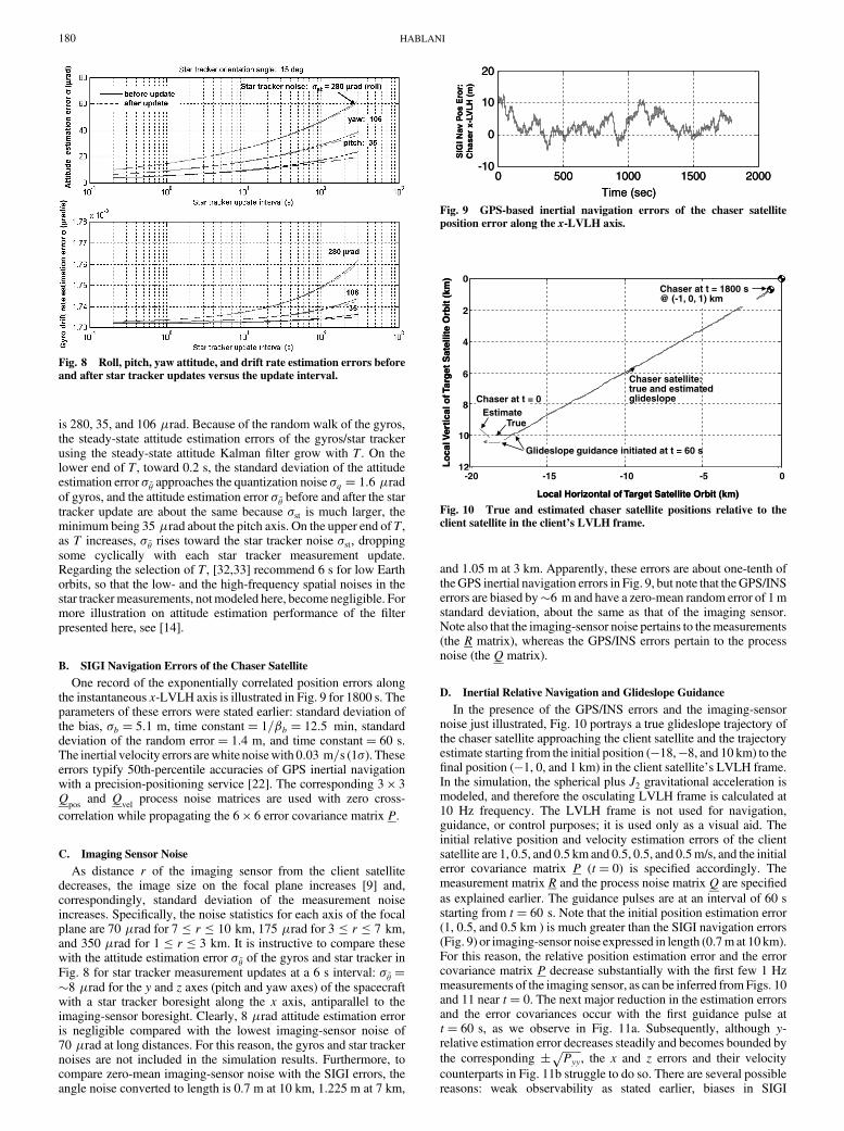
is 280, 35, and 106 �rad. Because of the random walk of the gyros,the steady-state attitude estimation errors of the gyros/star trackerusing the steady-state attitude Kalman filter grow with T. On thelower end of T, toward 0.2 s, the standard deviation of the attitudeestimation error � ~� approaches the quantization noise �q � 1:6 �radof gyros, and the attitude estimation error � ~� before and after the startracker update are about the same because �st is much larger, theminimum being 35 �rad about the pitch axis. On the upper end of T,as T increases, � ~� rises toward the star tracker noise �st, droppingsome cyclically with each star tracker measurement update.Regarding the selection of T, [32,33] recommend 6 s for low Earthorbits, so that the low- and the high-frequency spatial noises in thestar trackermeasurements, notmodeled here, become negligible. Formore illustration on attitude estimation performance of the filterpresented here, see [14].
B. SIGI Navigation Errors of the Chaser Satellite
One record of the exponentially correlated position errors alongthe instantaneous x-LVLH axis is illustrated in Fig. 9 for 1800 s. Theparameters of these errors were stated earlier: standard deviation ofthe bias, �b � 5:1 m, time constant� 1=�b � 12:5 min, standarddeviation of the random error� 1:4 m, and time constant� 60 s.The inertial velocity errors arewhite noisewith 0:03 m=s (1�). Theseerrors typify 50th-percentile accuracies of GPS inertial navigationwith a precision-positioning service [22]. The corresponding 3 � 3Q
posand Q
velprocess noise matrices are used with zero cross-
correlation while propagating the 6 � 6 error covariance matrix P.
C. Imaging Sensor Noise
As distance r of the imaging sensor from the client satellitedecreases, the image size on the focal plane increases [9] and,correspondingly, standard deviation of the measurement noiseincreases. Specifically, the noise statistics for each axis of the focalplane are 70 �rad for 7 r 10 km, 175 �rad for 3 r 7 km,and 350 �rad for 1 r 3 km. It is instructive to compare thesewith the attitude estimation error � ~� of the gyros and star tracker inFig. 8 for star tracker measurement updates at a 6 s interval: � ~� ��8 �rad for the y and z axes (pitch and yaw axes) of the spacecraftwith a star tracker boresight along the x axis, antiparallel to theimaging-sensor boresight. Clearly, 8 �rad attitude estimation erroris negligible compared with the lowest imaging-sensor noise of70 �rad at long distances. For this reason, the gyros and star trackernoises are not included in the simulation results. Furthermore, tocompare zero-mean imaging-sensor noise with the SIGI errors, theangle noise converted to length is 0.7 m at 10 km, 1.225 m at 7 km,
and 1.05 m at 3 km. Apparently, these errors are about one-tenth oftheGPS inertial navigation errors in Fig. 9, but note that theGPS/INSerrors are biased by�6 m and have a zero-mean random error of 1mstandard deviation, about the same as that of the imaging sensor.Note also that the imaging-sensor noise pertains to themeasurements(the R matrix), whereas the GPS/INS errors pertain to the processnoise (the Q matrix).
D. Inertial Relative Navigation and Glideslope Guidance
In the presence of the GPS/INS errors and the imaging-sensornoise just illustrated, Fig. 10 portrays a true glideslope trajectory ofthe chaser satellite approaching the client satellite and the trajectoryestimate starting from the initial position (�18,�8, and 10 km) to thefinal position (�1, 0, and 1 km) in the client satellite’s LVLH frame.In the simulation, the spherical plus J2 gravitational acceleration ismodeled, and therefore the osculating LVLH frame is calculated at10 Hz frequency. The LVLH frame is not used for navigation,guidance, or control purposes; it is used only as a visual aid. Theinitial relative position and velocity estimation errors of the clientsatellite are 1, 0.5, and 0.5 km and 0.5, 0.5, and 0.5m/s, and the initialerror covariance matrix P (t� 0) is specified accordingly. Themeasurement matrix R and the process noise matrix Q are specified
as explained earlier. The guidance pulses are at an interval of 60 sstarting from t� 60 s. Note that the initial position estimation error(1, 0.5, and 0.5 km ) is much greater than the SIGI navigation errors(Fig. 9) or imaging-sensor noise expressed in length (0.7m at 10 km).For this reason, the relative position estimation error and the errorcovariance matrix P decrease substantially with the first few 1 Hzmeasurements of the imaging sensor, as can be inferred fromFigs. 10and 11 near t� 0. The next major reduction in the estimation errorsand the error covariances occur with the first guidance pulse att� 60 s, as we observe in Fig. 11a. Subsequently, although y-relative estimation error decreases steadily and becomes bounded bythe corresponding �
�������Pyy
p, the x and z errors and their velocity
counterparts in Fig. 11b struggle to do so. There are several possiblereasons: weak observability as stated earlier, biases in SIGI
Fig. 8 Roll, pitch, yaw attitude, and drift rate estimation errors before
and after star tracker updates versus the update interval.
0 500 1000 1500 2000-10
0
10
20
Time (sec)
SIG
I Nav
Po
s E
ror:
Ch
aser
x-L
VL
H (
m)
0 500 1000 1500 2000-10
0
10
20
Time (sec)
SIG
I Nav
Po
s E
ror:
Ch
aser
x-L
VL
H (
m)
Fig. 9 GPS-based inertial navigation errors of the chaser satellite
position error along the x-LVLH axis.
TrueEstimate
Lo
cal V
erti
cal o
f Tar
get
Sat
ellit
e O
rbit
(km
)
Local Horizontal of Target Satellite Orbit (km)
Chaser at t = 1800 s@ (-1, 0, 1) km
Chaser at t = 0
Glideslope guidance initiated at t = 60 s
Chaser satellite:true and estimated glideslope
0
2
4
6
8
10
12-20 -15 -10 -5 0
TrueEstimate
Lo
cal V
erti
cal o
f Tar
get
Sat
ellit
e O
rbit
(km
)
Local Horizontal of Target Satellite Orbit (km)
Chaser at t = 1800 s@ (-1, 0, 1) km
Chaser at t = 0
Glideslope guidance initiated at t = 60 s
Chaser satellite:true and estimated glideslope
0
2
4
6
8
10
12-20 -15 -10 -5 0
Fig. 10 True and estimated chaser satellite positions relative to the
client satellite in the client’s LVLH frame.
180 HABLANI

navigation errors, lack of range measurements, a constantlyprecessing local LVLH frame due to the J2 effect, and the selectedQmatrix with qscalar � 0:001 not being tuned enough.
The components of the true and the estimated relative positionsand velocities of the chaser from the client spacecraft are shown inFigs. 12a and 12b. The exponential decrease of the relative positionto �1, 0, and 1 km in 1800 s is apparent. The relative velocity
components step up initially with the first guidance pulse at t� 60 sto suitable values to follow the stipulated glideslope guidance, andthen they are brought discretely and exponentially to the low valuesspecified at 1800 swith 29 periodicfirings at each 60 s interval. Thesecomponents of the �v pulses every 60 s in the LVLH frame areshown in Fig. 13, inwhichwe observe that thefirst pulse is the largestand the subsequent pulses are much smaller.
0 500 1000 1500 2000-2000
-1000
0
1000
0 500 1000 1500 2000-1000
-500
0
500
0 500 1000 1500 2000-500
0
500
0 500 1000 1500 2000-1
0
1
2
0 500 1000 1500 2000-1
0
1
2
0 500 1000 1500 2000-2
-1
0
1
0 500 1000 1500 2000-2000
-1000
0
1000
Time (sec)
x-re
l-est
err
or (
m)
0 500 1000 1500 2000-1000
-500
0
500
Time (sec)
y-re
l-est
err
or (
m)
0 500 1000 1500 2000-500
0
500
Time (sec)
z-re
l est
err
or (
m)
0 500 1000 1500 2000-1
0
1
2
Time (sec)
x-re
l vel
-est
err
or (
m/s
)
0 500 1000 1500 2000-1
0
1
2
Time (sec)
y-re
l vel
-est
err
or (
m/s
)
0 500 1000 1500 2000-2
-1
0
1
Time (sec)
z-re
l vel
est
err
or (
m/s
)
a) Relative position estimation error b) Relative velocity estimation error
Fig. 11 Estimation errors in the client’s LVLH frame, compared with corresponding � standard deviation.
0 500 1000 1500 2000-20
-10
0
Time (sec)
0 500 1000 1500 2000-10
-5
0
5
Time (sec)
0 500 1000 1500 20000
5
10
15
Time (sec)
0 500 1000 1500 2000-20
0
20
40
Time (sec)
0 500 1000 1500 2000-20
0
20
40
Time (sec)
0 500 1000 1500 2000-50
0
50
Time (sec)
x-re
lativ
e of
cha
ser
from
clie
nt (
km)
y-re
lativ
e of
cha
ser
from
clie
nt (
km)
z-re
lativ
e of
cha
ser
from
clie
nt (
km)
x-re
lativ
e an
d es
timat
e of
cha
ser
(m/s
)y-
rela
tive
and
estim
ate
of c
hase
r (m
/s)
z-re
lativ
e an
d es
timat
e of
cha
ser
(m/s
)
a) Relative position b) Relative velocity
true
true
true
estimate
estimate
estimate
Guidance pulses @ 60 s interval
Fig. 12 True and estimated relative position and relative velocity of the chaser in the client satellite’s LVLH frame; glideslope guidance is active.
HABLANI 181

E. Attitude Control and Stabilization of the Integrated Sensor’s Sight
Line
The inertial relative navigation and guidance performance justdiscussed is realized with a PID attitude controller of bandwidth0.064 Hz, equal to 360 times the orbital frequency, and samplingfrequency of 25 Hz (see Fig. 1). Reaction wheels are used asactuators. Hablani [14] presents a detailed pointing-accuracyanalysis and performance of the controller. Here, to conserve space,we limit the portrayal of performance to the focal-plane imagecoordinates expressed as angles of rotation about the focal-plane yand z axes. It is explained in Sec. IV that in the absence of allmeasurement noises and navigation errors, the focal-plane imageangles are, in fact, equal to the attitude control error signals about they and z axes: that is, �ey and �ez components of �e in Fig. 1. In reality,the attitude error signals and the actual focal-plane image anglesdiffer in some respects. Attitude error signal vector �e depends on theattitude command estimates and the attitude estimates, which areboth affected by the navigation errors and the gyro/star trackernoises, attenuated by the navigation Kalman filter and the attitudeKalman filter. The image on the focal plane, in contrast, exhibits alow-frequency motion because the focal plane (that is, its carrier, thespacecraft bus) is controlled by a low-bandwidth (0.064 Hz,corresponding to a period of 15.6 s) attitude controller. Thisdifference is seen in Fig. 14a, which depicts the two quantities for they axis with just the sensor noise. Whereas the image angle on thefocal plane about the y axis exhibits low-frequency, slightly growing,oscillation, the attitude error signal at 25 Hz has high-frequencycontents with amplitudes less than the amplitudes of the image angle.Figure 14b, on the other hand, shows the image angle and the attitudeerror about the y axis under SIGI navigation errors. We observe thatthe image angle (that is, the pointing error) is considerably larger thanthe focal-plane-noise standard deviation per axis (70–350 �rad forthe 10–1 km relative range), which steps up as the range decreases.Comparing the pointing accuracy in Fig. 14b with the pointingaccuracy in the absence of the SIGI navigation errors in Fig. 14a, weconclude that the image motion is mostly caused by the zero-mean
SIGI noise, with rms� 0:5–1:0 m causing a 100 �rad rms imagemotion at 10 km and a 1000 �rad rms at 1 km, agreeing with theresults seen in Fig. 14b. The bias position errors in the SIGInavigation errors of the chaser (Fig. 9), similar to the gyro and startracker misalignments in [14], do not offset the image from the focal-plane center.
Finally, Fig. 15 shows the root of the sumof squares (RSS) of the yand z image angles and compares it with the RSS of the imaging-sensor noise and the pointing-accuracy requirement for the laserrange finder to measure the relative range of the client satellite. Forthe range less than 12 km, the pointing-accuracy requirement of thelaser range finder is met only occasionally and, when met, a relativerange measurement arises. In the current simulation, this rangemeasurement is not used in the EKF, however; otherwise, the focal-plane pointing accuracy would improve further and enableprogressively more frequent range measurements.
VII. Conclusions
In this paper, a new sight-line-stabilized inertial relativenavigation system is presented for midrange (20–1 km) rendezvousof an active chaser satellite with a passive client satellite. The chasersatellite is stabilized to track the client satellite with an integrated
0 500 1000 1500 2000-20
0
20
40
Time (sec)
0 500 1000 1500 2000-20
0
20
40
Time (sec)
0 500 1000 1500 2000-40
-20
0
20
del v
z(m
/s)
del v
y(m
/s)
d
el v
Inbound glidescope
Time (sec)
x(m
/s)
Fig. 13 Glideslope guidance pulses in the client’s LVLH frame at 60 s
intervals for rendezvous.
Fig. 14 Elevation angle of the image on the focal plane (FP) andattitude control (AC) y error.
0 5 10 15 20 250
200
400
600
800
1000
Range to NS (km)
Foc
al P
lane
Imag
e R
adia
l Dis
tanc
e &
LRF
Poi
ntin
g A
ccur
acy
Req
mnt
. (µr
ad)
Imaging sensor
noise rms
Laser range finder pointing accuracy
requirement
Laser range finder pointing accuracy
requirement
Fig. 15 Target image RSS angle on the focal plane compared with
imaging-sensor measurement noise and laser range-finder pointingrequirement (NS is the client satellite).
182 HABLANI

sensor ensemble consisting of an imaging sensor, a coboresightedlaser range finder, the space-integrated GPS/INS (SIGI), and a startracker. A new six-state continuous-discrete extended Kalman filteris developed for inertial relative navigation of the client satellite. Asteady-state three-axis inertial attitude estimator is developed for thechaser satellite. The numerical results illustrate that this ensemblecarries out a successful midrange rendezvous solely with theazimuth- and elevation-angle measurements locating the clientsatellite without range measurements. The relative positionestimation errors are not necessarily within their standard deviationbounds, and in this respect, the relative navigation filter requiresfurther improvement. But this andMonteCarlo runsmust be deferredto future studies. Nonetheless, the attitude controller maintains theclient satellite within the imaging-sensor track box amidst the SIGInavigation errors and the client satellite’s location estimation errorsin the inertial frame. The pointing accuracy achieved with theimaging sensor enables the coboresighted laser range finder, whichrequires stringent pointing accuracy, to occasionally measure theinstantaneous range of the client satellite from the chaser satellite. Ifused by the relative navigation Kalman filter, these rangemeasurements would improve the pointing accuracy further andeffect more frequent range measurements, resulting in more accurateinertial relative navigation of the client satellite and guidance of thechaser satellite.
Acknowledgments
The work reported here was developed under the AutonomousVehicle Operations Research and Development program and theOrbital Express program. Manny R. Leinz, Anaheim, and RichardThiel, Huntington Beach, were the Chief Engineers of the twoprograms, respectively. The author is grateful for the opportunity tobe a member of their teams and for approval to publish this work.
References
[1] Bryan, T. C., “Automated Capture of Spacecraft,” AIAA SpacePrograms and Technologies Conference, Huntsville, AL, AIAAPaper 93-4757, Sept. 1993.
[2] Titterton, D. H., and Weston, J. L., Strapdown Inertial Navigation
Technology, Progress in Astronautics and Aeronautics, Vol. 207,AIAA, Reston, VA, 2004, pp. 475–479.
[3] Moir, I., and Seabridge, A., Military Avionics Systems, Wiley, NewYork, 2006, Sec. 5.7.
[4] Yim, J. R., Crassidis, J. L., and Junkins, J. L., “Autonomous OrbitNavigation of Two Spacecraft System Using Relative Line-of-SightVector Measurements,” American Astronautical Society, Paper 04-257, 2004.
[5] Hablani, H. B., “Autonomous Relative Navigation, AttitudeDetermination, Pointing and Tracking for Spacecraft Rendezvous,”Guidance, Navigation, and Control Conference, AIAA Paper 2003-5355, Aug. 2003.
[6] Kawano, I., Mokuno, M., Kassai, T., and Suzuki, T., “Results andEvaluation of Autonomous Rendezvous Docking Experiments of ETS-VII,” AIAA Guidance, Navigation, and Control Conference, Portland,Oregon, AIAA Paper 99-36780, Aug. 1999.
[7] Park, Y. W., Brazzell, J. P., Jr., Carpenter, J. S., Hinkel, H. D., andNewman, J. H., “Flight Test Results from Real-Time Relative GlobalPositioning System Flight Experiment on STS-69,” NASA TM104824, Nov. 1996.
[8] Clark, F. D., Spahar, P. T., Brazzell, J. P., Jr., and Hinkel, H. D., “Laser-Based Relative Navigation and Guidance for Space Shuttle ProximityOperations,” 26th Annual AAS Guidance and Control Conference,Breckinridge, CO, American Astronautical Society Paper 03-014,Feb. 2003, pp. 1–20.
[9] Gaylor, D. E., and Lightsey, E. G., “GPS/INS Kalman Filter Design forSpacecraft Operating in the Proximity of the International SpaceStation,” AIAA Guidance, Navigation, and Control Conference,
Austin, TX, AIAA 2003-5445, Aug. 2003.[10] Woffinden, D. C., andGeller, D. K., “Relative Angles-OnlyNavigation
and Pose Estimation for Autonomous Orbital Rendezvous,” Journal ofGuidance, Control, and Dynamics, Vol. 30, No. 5, 2007, pp. 1455–1469.doi:10.2514/1.28216
[11] Bauer, F. H., Hartman, K., and Lightsey, E. G., Spaceborne GPS:
Current Status and Future Visions, AIAA, Reston, VA, 1998.[12] Zubkow, Z., “Honeywell SIGI (Space Integrated GPS/INS) H-764G
System,” American Astronautical Society Paper 03-037, 2003.[13] Willms, R., “Space Integrated GPS/INS (SIGI) Navigation System for
Space Shuttle,” Inst. of Electrical and Electronics Engineers,Piscataway, NJ, 1999.
[14] Hablani, H. B., “Imaging Sensor Pointing and Tracking ControllerInsensitive to Gyros and Star Trackers Misalignments,” Journal of
Guidance, Control, and Dynamics, Vol. 31, No. 4, 2008, pp. 980–990.[15] Baiocco, P., and Sevaston, G., “On the Attitude Control of a High
Precision Space Interferometer,” Space Guidance, Control, and
Tracking, Vol. 1979, Society of Photo-Optical InstrumentationEngineers, Bellingham, WA, 1993, pp. 92–107.
[16] Hablani, H. B., Tapper, M. L., and Dana-Bashian, D. J., “Guidance andRelative Navigation for Autonomous Rendezvous in a Circular Orbit,”Journal of Guidance, Control, and Dynamics, Vol. 25, No. 3, 2002,pp. 553–562.
[17] Bar-Shalom, Y., Rong Li, X., and Kirubarajan, T., Estimation with
Applications to Tracking and Navigation, Wiley, New York, 2001,Sec. 3.7.
[18] Fogel, E., and Gavish, M., “N-th Dynamics Target Observability fromAngle Measurements,” IEEE Transactions on Aerospace and
Electronic Systems, Vol. 24, No. 3, May 1988, pp. 305–308.doi:10.1109/7.192098
[19] Van der Ha, J., and Mugellesi, R., “Analytic Models for RelativeMotion Under Constant Thrust,” Journal of Guidance, Control, and
Dynamics, Vol. 13, No. 4, 1990, pp. 644–650.doi:10.2514/3.25382
[20] Gelb, A., Applied Optimal Estimation, MIT Press, Cambridge, MA,1974.
[21] Markley, F. L., “Approximate Cartesian State Transition Matrix,”Journal of the Astronautical Sciences, Vol. 34, No. 2, Apr.–June 1986,pp. 161–169.
[22] Montenbruck, O., and Gill, E., Satellite Orbits: Models, Methods, and
Applications, Springer, New York, 2000, pp. 205, 293–302.[23] Misra, P., and Enge, P., Global Positioning System: Signals,
Measurements, and Performance, 2nd ed., Ganga-Jamuna Press,Lincoln, MA, 2006.
[24] Rogers, R. M.,Applied Mathematics in Integrated Navigation Systems,AIAA Education Series, AIAA, Reston, VA, 2003, pp. 190–206.
[25] Grewal, M. S., Weill, L. R., and Andrews, A. P., Global PositioningSystems, Inertial Navigation, and Integration, Wiley, NewYork, 2001.
[26] Katzman, M. (ed.), Laser Satellite Communications, Prentice–Hall,Upper Saddle River, NJ, 1987, Chap. 6.
[27] Pittelkau, M. E., “Rotation Vector in Attitude Estimation,” Journal ofGuidance, Control, and Dynamics, Vol. 26, No. 6, 2003, pp. 855–860.
[28] Reynolds, R.G., “Quaternion Parameterization and aSimpleAlgorithmfor Global Attitude Estimation,” Journal of Guidance, Control, and
Dynamics, Vol. 21, No. 4, 1998, pp. 669–671.[29] Markley, F. L., “Fast Quaternion Attitude Estimation from Two Vector
Measurements,” Journal ofGuidance, Control, andDynamics, Vol. 25,No. 2, 2002, pp. 411–414.
[30] Shneydor, N. A.,Missile Guidance and Pursuit Kinematics, Dynamics
and Control, Horwood Publishing, Chichester, England, U.K., 1998,pp. 217–218.
[31] Markely, F. L., and Reynolds, R. G., “Analytic Steady-State Accuracyof a Spacecraft Attitude Estimator,” Journal of Guidance, Control, andDynamics, Vol. 23, No. 6, 2000, pp. 1065–1067.
[32] Halsy, D. R., Strikewerda, T. E., Fisher, H. C., and Heyler, G. A.,“Attainable Pointing Accuracy with Star Trackers,” AmericanAstronautical Society Paper 98-072, 1998.
[33] Wu, Y. W., Li, R., and Robertson, A. D., “Precision AttitudeDetermination forGOESNSatellites,”AmericanAstronautical SocietyPaper 03-002, 2003.
HABLANI 183