available in pdf from //psych.nyu.edu/pelli/pubs/pelli1981thesis.pdf · available in pdf from ......
TRANSCRIPT

1981
Available in PDF from http://psych.nyu.edu/pelli/

EFFECTS OF VISUAL NOISE
Denis G. Pelli
Summary
Random fluctuation in luminance, over time or space or both, is luminance
noise. Squared threshold contrast is found to be proportional to the spectral
density of luminance noise, plus a constant. The constant is an estimate of
the observer's "equivalent noise". The observer's near-threshold performance
--at detection and discrimination (and possibly apparent-contrast matches) is
consistent with a description of the observer as noise-free except for the
equivalent noise at the visual field.
Effects of varying noise spectrum in all three spatia-temporal-frequency
dimensions support the hypothesis that we detect a grating by means of a linear
spatia-temporal filter, a "channel", so that squared threshold contrast is
proportional to the total noise power (including equivalent noise) passed by
the linear filter.
A hypothesis of intrinsic uncertainty leads to the channel-uncertainty
model, which is consistent with the noise effects and predicts summation and
facilitation effects as accurately as accurately as other theories which do not
explain the effects of noise. The uncertainty hypothesis was confirmed by
direct test: threshold contrast for one of ten-thousand possible signals was
only a factor of 1. 5 higher than threshold contrast of a fixed signal.

PREFACE AND ACKNOWLEDGEMENTS
The temporal-tuning data reported in Chapter 3 were collected in collaboration with A.B. Watson, with permission from the Board of Graduate Studies. Otherwise, this dissertation is the result of my own work and includes nothing which is the outcome of work done in collaboration.
Fergus W. Campbell, my PhD. supervisor, often disagreed with me, was usually right, but always let me find my own way. His keen curiousity and talent for dramatic demonstration of new understanding showed me how exciting research could be.
John G. Robson always seemed to know how an experiment would turn out, as though he had already done it years ago. He showed me how to fix a computer, design a video display, and how to approach any problem with the conviction that it can be solved without a degree in the specialty.
Gordon Legge, Dan Kersten, Gary Rubin, and Mary Schleske patiently listened again and again to my muddled explanations of what Rose meant by the "quantum efficiency of the eye", as I gradually determined how it was related to Barlow's quantum efficiency of the observer. They, Jamie Radner, and John Foley also provided helpful criticisms of my earlier drafts. I am grateful to Dan Kersten for acting as an observer in the experiment reported in Appendix 6.
My examiners, John G. Robson and Jacob Nachmias, made a number of important suggestions at my oral exam. In particular, I had not realized that channel-uncertainty is a form of probability summation.
I am grateful to the members and visitors of the Craik Laboratory for the stimulating environment they provided. I thank Clive Hood for his invaluable assistance. I am grateful to Robert Hess for many fruitful discussions on noise masking and for acting as observer in several of the experiments reported here. I am grateful to my friends A. "Beau" Watson, Dave C. Burr, and Andrew Dean for fruitful discussions, and collaborations on related projects. Roy Patterson of the MRC Applied Psychology Unit provided much helpful advice on off-frequency looking experiments, and helped me realize how worthwhile it might be to determine the predictions of the channel-uncertainty model. Correspondence with Arthur E. Burgess helped me to r~fine the ideas on efficiency.
Except for Appendix 6, all the experimental work was done at Cambridge University with support from a Ministry of Defense contract to F.W. Campbell entitled, "Spatial noise spectra and target detection/recognition". The writing, as well as the uncertainty experiment reported in Appendix 6, was done at University of Minnesota, where I was a Research Fellow and supported by Public Health Service Grant EY002934 to Gordon Legge.

TABLE OF CONTENTS
Chapter 1: Overview and Conclusions ••••••••••••••••••••••••••• 1
Chapter 2: Thresholds in White Noise ••••••••••••••••••••••••• 12
Chapter 3: Thresholds in Non-White Noise ••••••••••••••••••••• 86
Chapter 4: Effects of Noise-Masking and Contrast-Adaptation
on Contrast Discrimination and Apparent-Contrast
Ma tc he s • • • ••••••••••••••••••••••••••••••••••••••• 121
Chapter 5: Uncertainty in Visual Detection •••••••••••••••••• 129
Appendix 1: Characterizing Visual Noise •••••••••••••••••••••• 159
Appendix 2: Cross-correlation and Energy Detectors ••••••••••• 170
Appendix 3: The Effects of Heterodyne Noise •••••••••••••••••• 175
Appendix 4: Generating Narrow-Band Noise ••••••••••••••••••••• 179
Appendix 5: Off-Frequency Looking: Fitting the Curves •••••••• 185
Appendix 6: The Effect of Uncertainty: Detecting a
Signal at One of Ten-Thousand Possible
Times and Places ••••••••••••••••••••••••••••••••• 188
References ••••••••••••••••••••••••••••••••••••••••••••••••••• 196
CHAPTER 1
OVERVIEW AND CONCLUSIO.NS

CHAPTER 1: OVERVIEW AND CONCLUSIONS Page
OVERVIEW AND CONCLUSIONS
This chapter previews the important conclusions of the thesis, and
develops the notion of an observer's equivalent input noise. The observer's
equivalent input noise plays a key role in the interpretation of the empirical
findings.
Noise is an implicit part of most theories of visual detection, but little
is known of the nature of intrinsic noise, and little attention has been paid
to the studies of the effects of external noise. This thesis will consider the
effects of visual noise. The approach is analogous to the standard engineering
practice of describing, for exanple, an actual electronic amplifier as a "black
box" which is equivalent to an ideal noise-free amplifier with an equivalent
noise source added at its input. This is called, "referring the amplifier's
noise to its input~. The linearity of electronic amplifiers guarantees that
all the noise in an amplifier may be referred to its input. Electronics
manufacturers routinely publish the equivalent input noise spectra of their
products. Designers can directly compare the signals they want to use as
inputs with the equivalent input noise of the amplifier and determine several
kinds of signal-to-noise ratio. The equivalent input noise usually determines
the smallest signal the system can detect.
Luminance noise is random fluctuation in luminance over time or space, or
both. An observer's visual system has intrinisic sources of noise, including
that inherent in the probabilistic nature of light. This thesis will ask
whether the observer's intrinsic noise can be referred to his input; that is,
whether the observer acts as though he were noise-free except for an imputed
noise at his visual field. Historically the equivalent noise has been
described as a "dark light" which adds to the luminance function of the

<.;HAY.l't:H 1: UVJ::H Vlt:W ANU (.;UN(.;LU~lUN~ Page 2
stimulus to prduce the effective stimulus; here the equivalent noise will be
described as a contrast function which adds to the contrast function of the
stimulus to produce the effective stimulus.
Hecht, Schlaer, and Pirenne ( 1942) demonstrated that observers could
detect small brief flashes which sent an average of about 100 photons into the
eye. The observers' frequency-of-seeing curves were the same as that of an
ideal observer (looking through a neutral density filter) whose criterion for
responding "seen" was about 6 photons. As Barlow (1956) later noted, 6 photons
is only a lower bound on the number of photons the observers actually utilized;
any other source of variability could have limited the steepness of the
frequency of seeing curves.
Barlow (1956) went on to hypothesize a "dark light":
"One must accept the conclusion that the absorption of a single quantt.m ..£!!! excite a rod, and, • • • ·, one must also accept the conclusion that a threshold flash which is seen does cause two or more rods to be excited. Apparently, the limit to the sensitivity of vision does not lie in the rods but at a later point in the nervous pathway leading to consciousness. It would be surprising if there were no explanation for the failure to detect a single excited rod, and the performance of light-sensitive physical instrt.ments may provide a clue; here it is not the difficulty of amplifying weak signals that limits the sensitivity, but the difficulty of distinguishing a weak signal from the background of spurious signals, or 'noise,' which occurs without any light signal at all.
" [Noise could enter] the system anywhere between the stimulus and the final response, but if this noise is to set a limit to sensitivity it must enter the system before the level at which the threshold decision is made: this is the possibility which is pursued in this paper. Since the level of the threshold decision is not known, there is a strong case for considering first the effects of noise acting at the earliest possible point in the system - that is, to consider the effects of the rhodopsin molecule undergoing spontaneously the same reaction that occurs when it absorbs a quantt.m of 1 ight.

CHAPI'ER 1: OVERVIEW AND CONCLUSIONS Page 3
"The assumption to be examined is that events occur in the retina, or later in the pathway, which cannot be distinguised from the events which occur when light falls on the rods and a quant1.111 is· absorbed."
Barlow ( 1957) decided to treat this noise as a "dark light". We will shortly
take a different approach, but his analysis ·is instructive.
"The first step in the quantitative approach is to justify the choice of a unit to measure the retinal noise. Following the idea that it is related to Fechner's 'Augenschwarz' or the dark light of the eye, it is here expressed in units of light intensity. Thus if it is said that the dark light has a certain value, this means that a light of this intensity entering the eye would by itself cause the same amount of noise in the visual system that it is deduced to have in total darkness. This unit is derived f'ran the experimental measurements very directly, which is a strong reasons for choosing it • • • "
Since effective light level is the s1.111 of the dark light and any actual light,
it is expected that the actual light would be insignificant when it is much
less than the dark light and daninant when it is much greater than the dark
light. Since the data conform to this expectation it is reasonable to take the
light level at whfch the transition occurs as an estimate of the dark light.
" • • • to a first approximation, the [threshold] curves for different types of stimulus start to tt.irn upwards at the same value of background intensity. They differ in the slope of their rising portions, and a general approximate law seems to be that the increment threshold varies as some power of the background intensity; this power varies between 0. 5 and 1, but stays constant for any set of conditions over a moderate range just above threshold. Such a simple power law is represented by a straight line on the plot of log.AI against log I, and the noise level is very easily found by the intersection of this line with the ordinate corresponding to the absolute intensity which is equivalent to the dark light."
The notion of a dark light seems to be very helpful .in understanding
thresholds in the dark-adapted eye, but does not readily lend itself to
understanding thresholds at higher light levels. Conversely, the new
description of the equivalent noise as a contrast function, now to be
introduced, seems to be very helpful at non-zero light levels, but is undefined
in the dark. In the future it may be found fruitful to allow both types of

CHAFfER 1: OVERVIEW AHD CONCLUSIONS · Page 4
equivalent noise, extending the applicability of both ideas, but this thesis
will only con.sider the equivalent .noise as a contrast function •.
Equivalent~!!~ contrast function
Chapter 2 will review thresholds in luminance noise with a white
(i.e. flat) , spatio-temporal-ftoequency spectrum~ Many authors have determined
threshold contrasts for various patterns over a range of levels of white noise.
All report that for .each pattern the square qf the threshold contrast is
proportional to ~e sum ot the spectral density ot the noise mask and a
constant. The constant will be called the_ critical spectral density.
Zero-noise threshold will refer to the threshold contrast on a uniform f1eld.
The critical spectral den.sity is the spectral density at which the resulting
squared threshold is twice the squared zero-noise threshold. In this way one
can determine the critical spectral density of a white noise mask for any test
pattern. Figure 2. 1 is a typical graph of threshold contrast versus noise
• level • Both scales are logarithmic, but the threshold contrast scale is
expanded so that one log 1.11it of squared contrast (i.e. half a log unit of
contrast) has the same length as one log unit of noise level. The threshold
curve is flat for noise levels less than the critical noise level, and rises
with unit slope (indicating proportionality of squared threshold to noise
level) for noise levels greater than the critical noise level.
Chapter 2 will show that the critical spectral density is an estimate of
the observer's equivalent noise. Since the squared threshold is proportional
• !!.2.!!! level will be used synonymously with "spectral density" of noise.

Effect of spectral density
0 • 8cldeQ
X • 1 cldeg
I I I I
I I I I I I e) ; :
11111111 I lllllell
if tJ rl: Noise. spectral density [sec deg 1 ·
Signal Noise o-~o-Hz
•• "'n
•

CHAPTER 1: OVERVIEW AND CONCWSIONS Page 5
to the sum of the actual and critical noise levels it seems appropriate to call
the sum of actual and critical, the effective noise.!!.!!!· Even more useful is
the concept of the effective stimulus, defined as the sum of the contrast
function of the observer's equivalent noise and the contrast function of the
~timulus. The actual stimulus is a luminance function, and can be described by
a contrast function, but still has an associated luminance with a corresponding
level of photon noise. The effective stimulus has no luminance; it is solely a
contrast function, though it does include the observer's equivalent noise, some
part of which is due to photon noise.
The effective stimulus will allow us to partition the observer into two
parts, without making any asst.lllptions abo¢ his internal structure. The first
part, called "transduction" transforms the actual stimulus to the effective
stimulus. The second part, "calculation", transforms the effective stimulus
into th~ observer's performmce.
Much of Chapter 2 is devoted to establishing the conditions necessary to
satisfy the assumptions of TheQry of Signal Detectability, and thereby the
concepts of signal-to-noise ratio and efficiency. Efficiency of any
transformation is the squared ratio of the output signal-to-noise ratio to the
input signal-to-noise ratio. The theory of Signal Detectability guarantees
that eff!ciency cannot exceed 1. In the absence of luminance noise, the
overall efficiency of the observer, describing the efficiency of the
transformation from stimulus to the observer's performance, is Barlow's
"quantliD efficiency". In the absence of luminance noise, "transduction
efficiency" is the efficiency of the transformation from stimulus to effective
sttmulus. "Calculation efficiency" is the efficiency of the transformation
from effective stimulus to the observer's performance. QuantliD efficiency

CHAPTER 1: OVERVIEW AND CONCLUSIONS Page 6
equals the product of transduction efficiency and the calculation efficiency.
All three are measureable.
Chapter 3 will review thresholds in non-white noise. These data are
evidence for spatial-frequency channels. The threshold of an observer
detecting a sinusoidal grating is affected only by frequencies in the vicinity
of the test frequency. Detection is only hindered by noise within a band of
spatio-temporal frequencies about the signal frequency. This is consistent
with the established idea that detection is mediated by frequency selective
mechanisms, channels. The chapter will exanine the hypotheses that: 1. when
the observer is using a given channel, squared threshold is proportional to the
total noise power passed by a linear filter; 2. the signal determines which
~channel is used, regardless of the noise spectr\.111. Chapter 3 will present
' evidence in support of the first notion (squared threshold proportional to
total filtered-noise power), and some evidence that the second notion
(one-signal-one-channel) is not always true. It seems that the observer
learned to look off-frequency: using whichever channel gave the best
signal-to-noise ratio, and thus the lowest threshold.
Fortunately the channel tuning fUnctions are more or less s~etric about
the test frequency so the observer would not be expected to look off-frequency
when white-noise masks are used. By restric~ing ourselves to white noise masks
we may assume the observer always detects each grating by the same channel.
Chapter 3 presents much evidence in support of its hypothesis that for any
one channel, the squared threshold is·proportional to total filtered noise
power. This is analogous to Rushton's principle of univariance: the
photoreceptor response is selective by virtue of its absorption spectrum but
its response depends only on the number of photons absorbed, regardless of

CHAPTER 1: OVERVIEW AND CONCWSIONS Page 7
their spectra. In the same way the channel is selective by virtue of its
filter and its threshold seems to depend only on the noise power passed by the
filter, regardless of the noise spectrllll.
Additive intrinsic noise may occur at the input or output or within the
channel t s filter. Because or the channel t s univariance, threshold will depend
only on the resulting noise power at the filter output. Any l1.111inance noise
which produces the same noise power at the filter out put would have the same
effect on threshold as these intrinsic noises. Since the filter is linear, a
noise mask which doubles the squared threshold relative to the squared
zero-noise threshold also doubles the noise power at the filter output, and the
mask's contribution to the noise power filter output will be equal to that of
the intrinsic noise. Any noise spectrum could be used, but it is convenient to
use white noise. It was suggested above that the spectral density of white
noise which doubles the squared threshold be called the critical spectral
density. White noise at the critical spectral density is an equivalent input
noise for that channel.
or course intrinsic noise could instead be non-additive, or occur after
some nonlinear transformation of the channel filter output. In general such
noise could not be referred to the visual field; there may be no equivalent
input noise. Chapter 4 will present evidence from contrast discrimination for
such non-referable intrinsic noise, but it seems to be significant only well
above threshold. Threshold, and contrast discrimination near threshold, seem
to be determined by intrinsic noise that can be referred to the visual field.
Now consider all the channels taken together, that is, the observer. So
far we have considered equivalent input noises for each channel, but they may
differ. Can one noise spectrt.lll be found which serves as an equivalent input
CHAPI'ER 1: OVERVIEW AND CONCLUSIONS Page 8
noise for all channels? If so, the performance of an observer detecting
patterns on a blank or noisy backgrotmd could be accurately modeled by a
hypothetical noise-free observer with an equivalent noise at i~s field of view.
The problem is to find a spectrum for the equivalent noise that produces
in each channel the same variance that that channel's intrinsic noise produces.
Here is an exanple of why the existence of an equivalent input noise for each
channel does not imply the existence of an equivalent input noise for the
ensemble. Suppose two channels, A and B, are such that there is no frequency
to which both respond, and imagine a third channel, C, whose filter is the St.lll
of the f.il ters of channels A and B. Finally, suppose that channels A, B, and C
have the same intrinsic variance at their filter outputs. Any lt.lllinance noise
that produces the same variance in A and B will produce twice that variance in
C, thus there is no noise spectrun \oibich could serve as an equivalent input
noise for all three.
However such incompatibilities may not occur, so that an equivalent input
spectrt.ll'l could be fotmd f~r the ensemble of all channels. Then, in principle,
we could synthesize lt.111inance noise with that spectrt.ll'l. This noise should
raise the variance in every channel by the same proportion and therefore should
raise the threshold contrasts for all patterns by the same proportion. This
would be evidence that this is indeed an equivalent input noise for the
observer. Unforttmately it is exceedingly difficult to synthesize noise with
an arbitrary spatio-temporal spectrum.
Chapter 4 will exanine effects of white noise on matches of apparent
contrast and on contrast discrimination. The contrast of an unmasked match
grating was adjusted to match the apparent contrast of a test grating in noise.
At all noise levels, the match contrast was identical to the test contrast when

CHAPTER 1: OVERVIEW AND CONCLUSIONS Page 9
both were above their thresholds, but match contrast fell sharply to its
threshold When the test grating approached its threshold.
The results of contrast discrimination indicate that suprathreshold
contrast discrimination is limited by a non-referable intrinsic noise. For
suprathreshold contrasts the minimum discriminable contrast difference
increases with test contrast, and is independent of effective noise level.
Since the effective noise accounts for all referable noise, and suprathreshold
contrast discrimination is independent of effective noise it must be limited by
a non-referable intrinsic noise (or not limited by noise at all).
The utility of referring noise to the visual field is further enhanced by
evidence that near-threshold phenomena are scale-invariant. We have already
seen that the squared threshold is proportional to the eff~ctive noise level.
Chapter 5 presents evidence that for detection of a grating in noise the
psychometric function relating detectability to contrast is independent of
noise level if contrast is plotted in units of threshold contrast. Chapter 5
also replots results of Chapter 4 to show that for near-threshold test
contrasts, the relation of minimal detectable contrast difference to test
contrast is independent of noise level (when both contrasts are plotted in
units of threshold contrast). Near-threshold detectability and
discriminability depend only on the ratio of squared contrast to the effective
spectral density of the noise.
All the near-threshold phenomena reported here scale with the effective
noise level. Conversely, the suprathreshold phenomena reported (contrast
discrimination and apparent-contrast matches) are independent of the noise
level. The effective noise level seems to determine the limits of visibility,
with little or no effect above threshold. The equivalent-noise idea unifies

CHAPTER 1: OVERVIEW AND CONCLUSIONS
the explanation of near-threshold performance at all noise levels.
Suprathreshold phenomena will require separate explanation.
, Page 10
There are many models of the visual detection process that succeed in
relating one aspect of visual detection to another. From the steepness of the
psychometric fUnction the "probability summation" model predicts summation
effects (whereby extending a pattern, or combining disparate patterns increases
detectability slightly). From the steepness of the psychometric fUnction the
"nonlinear transducer" model predicts the facilitation observed in
near-threshold contrast discrimination. Neither model offers explanation for
the success of the equivalent noise description.
This thesis will present evidence that: 1. the noise in a channel relevant
to threshold can be referred to its input, and 2. the operation of the channel
scales with the effective noise level. These are severe constraints on models
of visual detection. For exanple, proponents of the standard version of
"probability summation" (which incorporates the "high-threshold" assumption)
will have to show how its intrinsic noise could be referred to the visual
field. Since in this model the intrinsic noise comes from the random failure
of channels to "detect", it is not clear how this could be done.
Many explanations have been offered for the steepness of the psychometric
fUnction. One of these, the "uncertainty hypothesis", is consistent with the
equivalent noise result. Chapter 5 will show that, with some simplifying
assumptions, this hypothesis implies that channel uncertainty should be an
accurate model of human performance. The model is based on the way an ideal
observer would detect one of many possible signals. The noise in this model
may be referred to its input, and the operation of the model scales with the
effective noise level. Furthermore it· will emerge that this model is both a

CHAPTER 1: OVERVIEW AND CONCLUSIONS Page 11
"probability summation" model (though without the high-threshold asslDllption)
and (as has been pointed out in the past). a "nonlinear transducer" model.
Calculations will be presented that show that this channel-uncertainty model
gives accurate, quantitative account of all the aspects of visual detection
mentioned above.
Finally, Appendix 6 (discussed in Chapter 5) will present an experiment
designed to test the uncertainty hypothesis: that the observer fails to make
full use of prior information about the identity of the signal. It was found
that the threshold contrast for a signal (a brief thin line) Which could appear
at any one of ten thousand possible times and places was only a factor of 1. 5
higher than when the observer lmew when and where it would be presented. The
small increase in threshold indicates that the observer benefits little from
the lmowledge o~ time and place, confirming the uncertainty hypothesis.

CHAPTER 2
THRESHOLDS IN WHITE NOISE

CHAPTER 2: THRESHOLDS IN WHITE NOISE Page 12
THRESHOLDS IN WHITE NOISE
ABSTRACT
Chapter 1 introduced the notion of the observer's equivalent noise. This chapter will show that study of the limitations of the human detection process is profitably divided into two parts. Firstly, what is the observer's ~quivalent noise level and what does it depend on? Secondly, given the effective noise level (the sum of the equivalent noise and any actual luminance noise), how well does the observer perform? The first question is addressed by the transduction efficiency, defined as the ratio of the photon noise to the observer's equivalent noise, or equivalently, the fraction of the corneal photons required to account for the observer's equivalent noise. Rose (1948) called it the "quantum efficiency of the eye". The second question is addressed by the calculation efficiency, defined as the observer's detective efficiency with respect to the "effective" signal-to-noise ratio. Barlow (1977) called it "central efficiency".
It is shown that (detective) quantum efficiency, QE, is the product of transduction efficiency, TE, and calculation efficiency, CE:
QE = TE X CE.
By a brilliant argument Rose (1948) concluded that our transduction efficiency ( "quantllll efficiency of the eye") is between • 5J and 5J for a wide range of patterns and luminances. However in order to reach this conclusion, he assumed that the calculation efficiency was constant. COnstancy of both transduction and calculation efficiencies implies constancy of quantum efficiency, i.e. the Rose-de Vries law, which was subsequently shown to be violated nearly everywhere (Barlow 1958). Assumption-free estimates of transduction efficiency made here from both published and new data are all between .4S and 3J. They span nearly 7 decades of light level, gratings of 2 to 15 c/deg, discs of 5. 7' to 32', and peripheral (7° nasal field) as well as foveal viewing. By implication, the failure of the Rose-de Vries law is due to changes of calculation efficiency, not transduction efficiency.
It is not generally appreciated that Rose (1946, 1948) introduced not one, but two fUndamental physical measures of light sensitivity. The first, quantum efficiency, which Rose applied to tv cameras and suggested applying to photographic film, has been widely applied to all image sensors including the human observer. Rose's second measure, which he called the "quantum efficiency of the eye" is here defined in a more general way and renamed "transduction efficiency". Like quantum efficiency it is a property of anything that is light-sensitive. It should be useful in sorting out the various causes of inefficiency in all complex light sensors, including the human observer, visually responsive cells, and photographic film.

CHAPTER 2: THRESHOLDS IN WHITE NOISE INTRODUCTION
INTRODUCTION
Page 13
This chapter will examine the effect of "white'' lllninance noise on the
contrast threshold. Report of new measurements will complement the first
thorough review of the existing literature. This chapter attempts to be
self-contained, but the reader may wish to refer occasionally to Appendix 1,
which presents a fuller explanation of the terms used to describe visual noise.
Luminance noise is random fluctuations in lllninance over space or time or both.
Contrast threshold refers to the amplitude (Lmax-Lmin)/(2lmean)1 of a pattern
which the observer can just detect well enough to satisfy some criterion of
response.
Only "white" noise will be considered. · Mathematicians sometimes define a
"white" noise process as having a constant spectral density at all frequencies,
but ·such a thing is physically impossible; infinite power would be required to
produce a non-infinitesimal spectral density over an infinite bandwidth. In
practice one studies mechanisms which are sensitive over only a finite
bandwidth, and there is no need to create the frequency components to which
there is no sensitivity. White noise here means that on each presentation
there was luminance noise whose frequency components over the bandwidth of the
mechanism under study, to a good approximation, had uncorrelated amplitudes
with equal variance and zero mean. As will be discussed in the following
pages, the goodness of the approximation was much better in some experiments,
and depends greatly on how one estimates the bandwidth of the mechanism under
study.
1 Since noise may be present, the L ax and lmtn that appear in this definition of signal contrast refer to the max~mum and m1nimum of the mathematically-expected luminance function on the signal-and-noise presentation.

CHAPTER 2: THRESHOLDS IN WHITE NOISE INTRODUCTION
Page 14
There are three reasons why the bulk of the thresholds-in-noise studies
used white noise: (1) theoretical convenience- several useful theorems in the
theory of signal detectability assume the noise is white; (2) as a simulation
of photon noise, or the actual noise encountered in image intensifiers or
television; and (3) technical limitations. It is fairly easy to produce one
or two-dimensional dynamic noise which is white (over some bandwidth). Other
spectra are much more difficult to achieve.
Figure 2.1 shows data I've collected which are representative of the
material to be reviewed later. Contrast threshold,~· (82S correct in 2IFC) is
plotted against n2 , the spectral density ~f the noise, for. two different test
patterns (sinusoidal gratings of 1 and 8 c/deg). The smooth curves drawn
through the data points represent the relation:
This relation has been found by everyone who measured contrast thresholds in
white noise. This chapter will review the evidence (in the Results and Review
sections) after considering the theoretical significance of the constants a and
b (in this section).
The constant of proportionality, ~· will be neglected for the moment.
From here on the constant b will be called the critical spectral density,
n~ritical' so we may rewrite our relation as,
C2 a: n2 2 critical + n •
The solid straight lines in Figure 2.1 represent the asymptotes of this
function. The horizontal line is the asymptote for noise levels approaching
zero; the unity-slope line is the asymptote for noise levels approaching

'0 0
~ .s:: .. ~ 1: 0•01 ·o u
Effect of spectral density
0 • 8c/deg
X • 1 c/deg
I
I I I
I I I I I e) I I
I I I I 111f I I I I llttl
if if ~:Noise spectral density [sec deg J
Signal Noise o-~OHz
~ y;~·~· t:7oms
,.....,
t-x·4" •• o-57 cldeg 4100CdJm2) NDP101-~
"ll ...... lQ c ,.., 11)
1\.)
•

CHAPTER 2: THRESHOLDS IN WHITE NOISE Page 15 INTRODUCTION
infinity. The lines intersect at the critical spectral density, n~ritical•
indicated by the dashed lines in the figure. The "critical" spectral density
is so called because it is the noise level above which threshold is primarily
2 determined by the luminance noise, n , and below which threshold is primarily
2 determined by the constant, ncritical•
In reviewing previous work we will need to consider two very different
techniques for generating the signal and noise. In experiments with continuous
displays, including mine, the signal-and-noise presentations were created by
adding a signal to what would have been a noise-only presentation, but this was
not true of the "dot" experiments. In the experiments using dot displays the
pattern was created by modulating the probability over space and/or time of a
Poisson source of identical small static or brief dots of light. Many dot
experiments were motivated by the need for empirical study of vision through an
image intensifier. Rose (1946, 1948) used a dot display as a simulation of
photon noise. van Meeteren and Boogaard (1973) gave a good description of the
appearance of such a dot, or "speck" display,
"Once detected by the photocathode .of electro-optical instruments, photons can be made visible as bright specks on an image screen by electronic amplification. When the detected photon flux is sufficiently high these specks combine in space and time to form a normal, smooth image. At lower light levels in object space, however, the detected photon flux can be so small, that the corresponding specks are visible as such, especially when the amplification is high."
others seem to have been motivated by the premise that dots "bypass early
levels of processing". Barlow (1978) discussed,
"the demonstration by French (1954), Julesz (1964), Uttal (1969) and others that patterns composed largely of random dots provide an opportunity to probe intermediate levels of processing in the visual system. The dots which compose the pattern are, it is suggested, reliably transduced and transmitted by the lower levels, and the limitations of performance result from the ways in which the nervous system can combine and compare groups of these dots at the next higher level."

CHAPTER 2: THRESHOLDS IN WHITE NOISE INTRODUCTION
Page 16
Even~so, except for the special case of countably few dots, available evidence
indicates that the effects of visual noise depend only on the noise spectrum,
and not on whether it is the result of dots or continuous luminance
fluctuation. By this interpretation, rather than bypassing anything, the dot
~isplays are simply sufficiently noisy to dwarf the noise sources that normally
limit detection.
Defining signal, noise, and the signal-to-noise ratio 2
In analyzing thresholds in noise we need to distinguish two cases
corresponding to the continuous and dot displays. In the continuous case the
signal was added to an independent noise (i.e. a continuous display). In the
Poisson case the signal modulated the prior probability (over space and/or
time) of random dots (i.e. a dot display) or photons (i.e. a noise-free
display). The continuous noise is characterized by its spectral density,
n2 (f), and the Poisson noise is characterized by the event rate, Jdots• or
Jphotons. Event rate will be used as a general term to refer to the density of
static dots (in dots per deg2 ) or flux of dynamic dots or "specks" (in dots per
deg2 sec) or photon flux (i.e. the retinal illuminance, in photons per deg2
sec). Because of this dichotomy there has been a tendency to view continuous
and dot experiments as very different. By applying a uniform terminology to
both sorts of experiments it will be seen that the results are very similar,
except in the few cases of countably few dots, discussed at the end of this
chapter. Appendix 1 shows that the spectral density n2 of Poisson events is
2 The rest of this introduction is devoted to establishing the vocabulary to be used in the Results and Review sections. This section complements Appendix 1; the molecules defined here are made up of the atoms defined there. The reader may prefer to skip directly to the Results section and refer back to here and to Appendix 1 as needed. To make this easier all defining instances are underlined.

CHAPTER 2: THRESHOLDS IN WHITE NOISE INTRODUCTION
the reciprocal of the event rate, J,·
n2 = 1/J.
Page 17
The Results section will show that continuous and dot experiments produce
similar graphs of threshold versus noise spectral density.
We need to establish a vocabulary which can be applied to both the
continuous and Poisson cases. The experiments all sought some measure of the
signal strength necessary for the observer to distinguish noise-only
presentations, which were purely random, from signal-and-noise presentations,
where some simple known pattern (the "signal") was present amidst the
randomness.
Each noise-only presentation has a luminance function ~N(x,y,t) randomly
drawn from the noise-only ensemble of possibilities, and each signal-and-noise
presentation has a luminance function ~N(x,y,t) randomly drawn from the
signal-and-noise ensemble of possibilities. FolloWing Linfoot (1964) define a
contrast function as the luminance function divided by the mean luminance,
minus one. The contrast functions of the two types of presentation are
and
~(x,y,t)
cN(x,y,t) = ----- 1 Lmean
LsN<x,y,t) cSN{x ,y, t) = .,.----- - 1,
lmean
where Lmean is the mean luminance on the noise-only presentations. Define
noise{x,y,t) as the contrast function of the noise-only presentation:

CHAPTER 2: THRESHOLDS IN WHITE NOISE INTRODUCTION
noise(x,y,t) = cN(x,y,t).
Page 18
The contrast function of the noise, noise(x,y,t), is random, different on every
presentation. Define the signal fUnction signal(x,y,t) as the difference
between the expected 1 contrast functions on signal-and-noise presentations and
on noise-only presentations.
signal(x,y,t) = <csN<x,y,t)> - <cN(x,y,t)>
The signal fUnction is fixed, identical on every signal-and-noise presentation.
For example, in Figure 2.1 the signal fUnction of the 8 c/deg grating is
-(~)2-<&>2-(~)2 signal(x,y,t) = c e •5 7 ms sin(2 8cycle x)
,.. degree •
In the continuous case (including my experiments) the contrast function of the
signal-and-noise presentation was the sum of the contrast function of the
signal and the contrast function of the noise:
cSN = signal(x,y,t) + noise(x,y,t).
In the Poisson case the contrast function of the signal-and-noise presentation
differs slightly from the sum of the contrast function of the signal and the
contrast function of the noise:
cSN ~ signal(x,y,t) + noise(x,y,t),
but we will shortly see that we may usually ignore the.discrepancy. In terms
of the contrast functions we have just defined, the original luminance
functions are
1 Expected means the average over the ensemble of possible luminance functions for that type of presentation (i.e. noise-only or signal-and-noise). This operation will be symbolized by angle brackets, < >.

CHAPTER 2: THRESHOLDS IN WHITE NOISE INTRODUCTION
LN(x,y,t) = Lmean x [1 + noise(x,y,t)]
and
Page 19
LSN(x,y,t) ~ Lmean x [1 + signal(x,y,t) + noise(x,y,t)].
The constant of proportionality in the relation
is a measure of efficiency of detection. There is a body of theorems called
Theory of Signal Detectability which establish the ideal performance attainable
in various tasks involving detection of a signal in additive, Gaussian, white
noise (Peterson, Birdsall, and Fox 1954). These theorems show that the
detectability of a known signal by an ideal observer depends only on a
dimensionless quantity called the signal-to-noise ratio, s/n, where .!!. is the
positive square root of n2, the spectral density. I will shortly define the
"signal energy" s2.,. The original definitions are all for functions of only one
dimension, time. We will want to consider ideal detection of signals in noise
of several dimensions, particularly dynamic, two-dimensional, white noise.
The contrast, ~, of a contrast function is half its peak-to-peak
amplitude. 5 The power, c;ms' of a contrast function is its variance,
,. The symbols s 2, n2 , and s/n are my notation. The conventional symbols, E, N012, and ,1(2E/N0), were developed for functions of one dimension (time~ and bec~e very clumsy if generalized to functions of k dimensions: E, N0/2 , and ,1(2 E/N0). See Appendix 1.
5 This follows from the (L -L t )/L definition of contrast, and the . max m n mean defin1tion of the contrast t-unc~ on.

CHAPTER 2: THRESHOLDS IN WHITE NOISE INTRODUCTION
Page 20
i.e. average squared value. The signal energy, s 2 , is the integral of the
squared signal fUnction along the dimensions of random variation of the noise.'
For example, if the noise is two-dimensional, dynamic, white noise, the signal
energy is integrated over all space (i.e. the visual field) and time:
If the noise is two-dimensional, static, white noise, the signal energy is
integrated over the visual field:
6 This definition is clumsy because I wish to include noise which is white over various numbers of dimensions. When the noise is two-dimensional dynamic white noise my definition reduces to that used by Watson, Robson, and Barlow (1981) who define "contrast energy" of a contrast function as the product of its power and area and duration, i.e. the integral of the squared contrast function over space and time. Similarly, for static two-dimensional white noise my definition reduces to Linfoot's (1964) integral of the squared contrast function over space. It is the dimensionless signal-to-noise ratio that is the f~ndamental quantity. A more gene~al treatment would allow any noise spectrum, n. (fx,fy,ft) and signal spectrum S (fx,fy,ft) and define the squared s1gnal-to-noise ratio as
2 S (fx,fy,ft) = J+m J+m J+m dfx df df
-m -m -m 2 y t • n (fx,fy,ft)
( s/n) 2
This definition shows that the signal-to-noise ratio will be infinite if the signal has energy at any frequency at which there is no noise. The disadvantage of the general approach, for our purposes, is that the concept of signal energy is lost entirely. The compromise taken in this chapter has been to restrict the noise to be white in the dimensions in which the noise has random variation. Because of that restriction, the definition of signal energy adopted in this chapter will give us the same signal-to-noise ratio as the more general definition.
CHAPTER 2: THRESHOLDS IN WHITE NOISE INTRODUCTION
Page 21
For many purposes it will be sufficient to use the fact that signal energy is
proportional to squared contrast,
without going to the trouble to calculate the signal energy.
The Theory of Signal Detectability established the ideal detectability of
signals in additive Gaussian white noise. Rose (1942, 1948) and de Vries
(1943) deyeloped fluctuation theory to handle the Poisson case'. The
signal-to-noise ratio in the Theory of Signal Detectability is a great
convenience: in the context of a detection experiment the stimuli may be
characterized by the signal-to-noise ratio, and the observer's performance at
many tasks may be characterized by the signal-to-noise ratio, d', that an ideal
observer would require to perform equally well.' Corresponding theorems have
not been developed for the Poisson case, and in general treatments of the
Poisson case there is nothing even analogous to a signal-to-noise ratio. For
example Barlow (1977) defines "quantum efficiency" as "the minimum proportion
of quanta entering the eye that would enable the task to be performed."
However, because it is so useful to have a single parameter to characterize
' Fluctuation theory corresponds more closely to Signal Detection Theory (SOT, e.g. Green and Swets 1966) than to Theory of Signal Detectability (TSD, e.g. Peterson, Birdsall, and Fox 1954). Fluctuation theory and SOT both draw on proofs about ideal detectability to make models of human performance, often modified to take account of our imperfections. Thus while the TSD and Poisson-case theorems (e.g. Thibos, Levick, and Cohn 1979) about ideal detectability are unlikely to be wrong, fluctuation theory and SOT are speculative models of human behavior, and like most models, probably are wrong.
1 This is Tanner and Birdsall's (1958) definition of d', not Green and Swets's ( 1966), but the two are numerically equal for the purposes of this chapter.

CHAPTER 2: THRESHOLDS IN WHITE NOISE INTRODUCTION
Page 22"
ideal detectability, fluctuation theorists usually make some approximations
which allow them to calculate a signal-to-noise ratio.
Consider ideal detection of a bright disc of contrast c, area A, and
duration T, on a dot display with average dot rate J {e.g. dots per deg2 sec).
The analysis would be identical for a display with no luminance noise,
exchanging the word "photon" for "dot". The ideal detector would count the
number of dots arriving in the area and duration corresponding to the signal.
The count on a noise-only presentation has mean and variance ATJ; the count on
a signal-and-noise presentation has mean and variance ATJ+2cATJ. 9 An exact
calculation would determine the performance attainable from decisions based on
these Poisson random variables. However, if ATJ is large the counts will, by
the Central Limit theorem, have nearly Gaussian distributions, and if the
contrast is low the variances of the two counts {N and SN) will be negligibly
different {Cohn, Green, and Tanner 1975). With these approximations the
performance of the ideal depends only on the mean di.fference 2cAT J in units of
the common standard deviation I{ATJ),
l1 2cATJ 0 = I(ATJ)= 2ci{ATJ).
Thus fluctuation theorists determine a "signal-to-noise ratio": the mean number
of extra photons in the signal divided by the standard deviation of the
noise-only count.
This is identical to the signal-to-noise ratio s/n that we would have
calculated if we had applied our definitions of signal energy, s 2, and noise
9 The factor of 2 that appears here and throughout the rest of the calculation results from the definition of contrast as {Lmax-~in)/~ean• so that
~L/Lmean = 2c •
CHAPTER 2: THRESHOLDS IN WHITE NOISE Page 23 INTRODUCTION
spectral density, n2, in the first place. The signal energy is s 2:(2c}2AT, the
noise spectral density is n2:1/J, and so the signal-to-noise ratio is
s 2c.AAT} ii = ,t(i/J) = 2c.t(ATJ}.
1his shows that s/n is an important quantity, but we can do better. By
considering the limits of the observer (that is, the bandwidth of the mechanism
under study} we can show that the basic assumptions of Theory of Signal
Detectability are usually satisfied to a good approximation by both continuous
and dot displays. Then we can conclude that the signal's ideal detectability
depends only on the signal-to-noise ratio, s/n. We must establish the validity
of applying theorems which assume additive, Gaussian, white noise to
experiments in which the noise was non-Gaussian, and in some cases(the dot
experiments} non-additive.
The discrepancy between the noise assumed in theory and used in practice
results in part from physical constraints on luminance displays. For exanple,
a Gaussian amplitude distribution would require an infinite dynamic range, but
excursions from the mean luminance on any actual display have some positive
limit, and negative excursions cannot go below zero luminance. However we can
make use of the fact that the observer is only sensitive over a finite
bandWidth of spatial and temporal frequencies to show that the effect of the
experimentally produced noise is the same as that of the noise assumed in the
theory. In the same way that a small aperture 1 imits the resolution of a
camera, the finite bandwidth of a mechanism under study limits its resolving
power. If the sample density (or dot flux} is many times the bandwidth of the
mechanism under study then the mechanism cannot resolve individual samples (or
dots} and responds only to weighted sums over many samples. The amplitude
distribution of these sums, in accord with the Central Limit Theorem,

CHAPTER 2: THRESHOLDS IN WHITE NOISE Page 24 INTRODUCTION
approaches Gaussian form. If the sample density is many times the bandwidth of
the mechanism und.er study then the effects of the noise depend only on its
spectrum n2 (f) over the frequencies of interest. Thus the validity of the
continuous Gaussian noise assumption rests on establishing a low upper bound
estimate of the bandwidth of the mechanism under study. We could
conservatively estimate this bandwidth as the bandwidth of the observer, but
there is evidence that the performance of an observer detecting a given signal
is .affected only by noise within a much narrower bandwidth.
Let us take Robson's (1966) contrast sensitivity function over
spatio-temporal frequency to estimate the observer's (two-sided) bandwidth at
about 2x30 c/deg X 2x30 c/deg X 2x30 Hz m 200,000 per deg2sec. On this basis
.we can expect that the observer will be unable to distinguish dot fluxes large
relative to 200,000 per deg2sec from continuous noise with the same spectral
density. Alternatively we could use the evidence discussed in Chapter 3 that
the threshold of an observer detecting a grating is affected only by noise in
the vicinity of the grating frequency, to estimate the bandwidth of a
hypothetical, tuned mechanism, a "channel", which mediates detection. Though
the experimental techniques were varied, the derived bandwidths are suitable
for at least a rough calculation. These bandwidths are ±1 octave about the
spatial frequency of a signal grating, .6 c/deg orthogonally, and about 16Hz
temporally. For a 4 c/deg grating, the product would be 2x6 c/deg x 2x.6 c/deg
x 2x16 Hz m 500 per deg2sec. Thus on the basis of the noise-masking results of
Chapter 3 we would expect the mechanism that mediates detection of 4 c/deg to
be equally affected by dot fluxes large relative to 500 per deg2sec and
continuous noise with the same spectral density. For a static dot display
similar calculations yield a (two-sided) bandwidth of about 4,000 per deg2 for
the observer, and 14 per deg2 for a 4 c/deg channel. The Results section will

CHAPTER 2: THRESHOLDS IN WHITE NOISE Page 25 INTRODUCTION
show that thresholds in continuous and dot noise are very similar for dot
fluxes down to several hundred dynamic dots per deg2sec, and about 18 static
dots per deg2 suggesting that the channel bandwidth, not the observer's
bandwidth is what matters. Below these dot fluxes and densities observers are
much more accurate, and it has been suggested that they base their decisions on
numerical estimates of dot nllllber.
One of the results of explicit consideration of the finite-bandwidth of
the mechanism under study is that contrast is an inappropriate measure of
wide-band noise. It was mentioned above that a finite bandwidth mechanism
cannot distinguish between the noises actually used, which had finite contrast,
and noise with a Gaussian amplitude distribution and infinite bandwidth, whose
contrast would be infinite. Stimuli whose bandwidth are narrow relative to the
mechanism under study may be usefully characterized by their power, c~s' or
rms contrast crms; stimuli whose bandwidths are broad relative to the mechanism
under study are characterized by their spectral density n2(f).
In~the Poisson case the observer must detect the relative increase or
decrease in events (dots or photons) in some areas due to the "signal". The
likelihood of an event in a given part of the fi~ld is determined by a prior
probability. In noise-only presentations the events can appear anywhere over
the field with equal prior probability. In the signal-and-noise presentations
the prior probability is modulated by the signal fUnction, signal(x,y,t).
The contrast functions of the signal and noise are not additive in the
Poisson case. The spectral density of the noise-only presentation is given by
1/J, the reciprocal of the event flux, but in the signal-and-noise presentation
the event flux is modulated by the signal and therefore the spectral density of
the noise is modulated too. In principle this could be relevant to detection,

CHAPTER 2: THRESHOLDS IN WHITE NOISE INTRODUCTION
Page 26
i.e. distinguishing signal-and-noise from noise-only presentations. Since most
or the signal contrasts (and noise modulation) were below 10S 11 , the modulation
or noise spectral density will be neglected, so that we may assume additivity
or the signal and noise.c
Thus we have seen, firstly, that the theoretical assumption that the noise
is white requires that noise in our experiments have a constant spectral
density over the bandwidth of the mechanism under study, which may be much less
than the observer's bandwidth. Secondly, the theoretical assumption that the
noise is Gaussian requires that we use a sample flux much greater than the
bandwidth of the mechanism under study. Finally, the theoretical assumption of
additivity of signal and noise is not quite satisfied in the Poisson case, but
at low signal contrasts the discrepancy is probably negligible. As we will see
in the Review, these expectations are confirmed by the essentially identical
results with continuous and dot experiments.
Now we can introduce~. the signal-to-noise ratio, s/n, that would be
required by an ideal observer to perform as well as the observer under study
(Tanner and Birdsall 1958) 11 • d' may be calculated, for example, from the
proportion correct of 2IFC responses, or from the hit and false-alarm rates of
yes-no responses.
1 0 Apparently no one has measured how well we detect modulation of rms noise contrast.. Dudley (personal communication) of the Royal Aircraft Establishment, Farnb9rough, England, has suggested it may be an important cue in detecting targets on image intensifiers (N'lich are dot displays). But this seems unlikely. Extrapolating from detection of contrast increments of sinusoidal gratings would suggest a Weber fraction (i.e. threshold increment as a fraction of the background) no less than 30S. Since the spectral density of the noise is pro~rtional to contrast squared, this would correspond to a (1.3/1) ~1.5-fold increase, or a 50S Weber fraction of spectral density. This suggests that the lOS modulation caused by a signal at 10S contrast is utterly undetectable by the observer.

CHAPTER 2: THRESHOLDS IN WHITE NOISE INTRODUCTION
Efficiency
Conceptually, the "efficiency" of a detector is the squared
signal-to-poise ratio of its output, (s/n)~ut• divided by the squared
2 signal-to-noise ratio at its input, (s/n)in'
( s/n)~ut
2 ( s/n)in
Page 27
It is important to realize that the reward for our labor in establishing the
applicability of Theory of Signal Detectability is the knowledge that no
transformation can increase a signal-to-noise ratio. Efficiency cannot exceed
1.
The output is often not of the same nature as the input (e.g. the I
observer's responses have little resemblance to the pattern he may be
detecting) so that it is not obvious how to calculate the output
signal-to-noise ratio. Efficiency is defined as the ratio of the squared
signal-to-noise ratio which would have been required by an ideal device for the
observed performance, divided by the squared signal-to-noise ratio at input
(Tanner and Birdsall 1958),
Efficiency = ( s/n)fdeal
( s/n)~n
11 This is not the same as Green and Swets's (1966) definition which treats the ideal observer (of a signal known exactly) as a model of the human, observer and then defines d' as a parameter ·of the internal statistics of that model. Green and Swets's definition would be unsatisfactory for our current purposes because it would make our conclusions appear to depend on the validity of an unlikely model. The two definitions of d' are n1.1nerically equal for exactly known signal, so the calculations in this chapter would be the same for either definition, but differences will appear in Chapter 5, which considers detection of signals not known exactly.

CHAPTER 2: THRESHOLDS IN WHITE NOISE INTRODUCTION
Page 28
We have already defined d' as the signal-to-noise ratio the ideal would have
required:
d' = (s/n)ideal'
so we can write the definition of efficiency more concisely as
Efficiency =
where the subscript "in" has been dropped because it is implied anyway.
Since the efficiency definition depends only on a ratio including signal
energies and noise levels we may equate either the signal energies or noise
levels without constraining the ratio that defines efficiency. If we equate
the noise levels the efficiency is the ratio of signal energies:
Effie iency = s2 I 2 ideal n
s2/n2 =
In fact this is Tanner and Birdsall's (1958) original definition of
("detective") efficiency. the fraction of the energy made available which is
ideally required.
Similarly we may equate the signal energies and write efficiency as a
ratio of noise levels:
Efficiency 2 2
s /nideal = --,.--
s2/n2
n2 =---
n2 ideal
If the input is made up of discrete stochastically independent (Poisson) events I
then we may equate the signal energies and use the equality of spectral density

CHAPTER 2: THRESHOLDS IN WHITE NOISE Page 29 INTRODUCTION
and reciprocal event rate,
2 n = 1 /J,
to write efficiency as a ratio of event rates:
n2 Jideal
Efficiency = = n2 J ideal
Calculation efficiency
Let us call the sum of actual and equivalent noise levels the effective
noise level. 2 Since in practice we estimate the equivalent noise by ncritical
we have
n2 = n2 + n2 effect! ve critical'
so our relation,
C2 « n2 2 critical + n '
can be more succinctly stated as proportionality of squared threshold to
effective noise level,
Define the effective signal-to-noise ratio as the square root of the ratio
of signal energy to effective noise spectral density,
2 s 2 s 2 (s/n)effective = -n-2---- = -2-----~2.
effective ncri tical + n

CHAPTER 2: THRESHOLDS IN WHITE NOISE INTRODUCTION
Page 30
Define the Calculation Efficiency, CE, as the ratio of the squared signal-to-noise ratio which would have been required by an ideal device for the observed performance, divided by the squared effective signal-to-noise ratio at input,
(d')2 (d')2 CE : ----~------- = ~--~----------~
( s/n)2 2/(n2 + n2). effective s critical
Define the effective stimulus as the sum of (the contrast function of) the
observer's equivalent noise and (the contrast function of) the actual stimulus.
The calculation efficiency measures the observer's performance relative to how
well an ideal observer would perform in response to the effective stimuli.
Returning to our empirical relation,
c2 « n2 effective'
we may replace the squared contrast c2 by the signal energy s 2, since they are
proportional to each other, to get
s2 « n2 . effective•
so their ratio, (s/n);ffective• is constant. Furthermore, threshold in each
data set that we will consider either corresponds to a constant d', or, in the
case of method-of-adjustment thresholds, we might suppose it does. So we may
write
(d')2 constant = -------------
(s/n)2 ' effective
but this is the calculation efficiency, CE. So our relation is just the
finding that the calculation efficiency is constant:

CHAPTER 2: THRESHOLDS IN WHITE NOISE INTRODUCTION
constant = CE.
Page 31
In general the constant will depend on d'. Thus, the empirical t.lnding is that
for a given d' the calculation efficiency is independent of the noise level,
2 2 2 n • At high noise levels, n >>ncritical' the detective and calculation
efficiencies will be asymptotically equal.
So far we have observed that the data in Figure 2. 1 were described well by
the relation
2 - 2 2 c - ncritical + n •
The definition of calculation efficiency may be rearranged to write
This redeems the promise to explain the additive constant (it is n~ritical>
and the proportionality constant (explained by CE) of the linear relation found
between squared contrast and noise level.
Transduction and quantum efficiencies
Having referred the observer's noise to his visual t.leld we may now ~sk
what is responsible for it. Is it due to photon noise?
Let Jphotons represent the retinal illuminance in corneal 12 photons per
sec deg2• 1 ' It is shown in Appendix 1 that a distribution made up of many
independent (Poisson) events has a white spatio-temporal spectrum and a
spectral density equal to the reciprocal of the event rate. The noise results
from the probabilistic way that light is absorbed and emitted by matter, in

CHAPTER 2: THRESHOLDS IN WHITE NOISE INTRODUCTION
Page 32
this case our photoreceptors, so that a uniform retinal illuminance results in
a noisy photon flux. We don't know what fraction of the photons is absorbed -
to some extent that is the purpose of the enterprise - but we can calculate a
minimum noise level corresponding to complete utilization. Define the photon
noise, n2 as that minimum noise level: photons•
n2 = 1 /J photons photons
An otherwise noise-free device that used all the photons would have an
equivalent input noise,
if it used half the photons its equivalent noise would be twice that,
2 2 1 ncritical=2nphotons= 1 /(~photons>·
2 Thus it seems reasonable to call the ratio of the photon noise nphotons to the
observer's equivalent noise, his "transduction efficiency", "TE". The observer
may in fact absorb more photons but he must absorb at least the fraction TE of
the photons for his equivalent noise to be as low as it is. By the end of this
12 Corneal photons are those photons which arrive at the observer's cornea(s) and will not be blocked by his iris(es). We will follow Barlow (1962a) and count all corneal photons, whether presented monocularly, or distributed binocularly to both the observer's eyes. This will make it necessary to halve quantum efficiency estimates such as those of Rose (1948) or Jones (1959) which neglected the light gathered by the observer's second eye.
11 If the light is not monochromatic it is conventional to base quantum efficiency calculations on the photon flux at the wavelength of maximum sensitivity (i.e. 507 nm for scotopic vision, 555 nm for photopic vision) which would produce the same photopic or scotopic retinal illuminance. Scotopically we are monochromats, and the equivalence follows. Photopically, van Nes and Bouman (1967) have shown that threshold contrasts of sinusoidal gratings (.5 to 50 c/deg) were the same (after correcting for the dependence of diffraction on wavelength) in red, green, and blue monochromatic lights equated for photopic luminance by flicker photometry.

CHAPTER 2: THRESHOLDS IN WHITE NOISE INTRODUCTION
Page 33
section it should be clear to the reader that transduction efficiency is what
Rose (1946, 1948) called the "quantum efficiency or the eye". Rose (1948)
claimed our transduction efficiency was between .5S and 5S (for white light)
for a wide range or conditions. Surprisingly there is still little evidence on this
point, but we will see that available evidence yields estimates or the
transduction efficiency that all lie between .4S and 3S (at 555 nm) for a wide
range or patterns and luminances, in remarkably good agreement with Rose's
claim.
The notions or transduction and quantum efficiency have an interesting
history which will shortly be recounted. However it will be best to begin with
a theoretical framework.
Quantum efficiency, QE, is efficiency o.r performance with respect to input
in the case where the input noise is just photon noise,
(d' )2
QE = ---2---. ( s/n)photons
As in the general case we may fix the signal energy and rewrite the quantum
efficiency as
QE: Jideal
Jphotons
which is "the minimum proportion or quanta entering the eye that would enable
the task to be performed" (Barlow 1977).
Quantum efficiency (also called "detective quantum efficiency" 1 -), is now
the principal index of performance of light transducers in many fields.
Apparently Rose (1946) invented it. This will be discussed fUrther in the

CHAPTER 2: THRESHOLDS IN WHITE NOISE INTRODUCTION
History sub-section.
Page 34
Calculation efficiency, f!, is efficiency of performance with respect to
the effective signal-to-noise ratio:
(d' )2
CE =--~--(s/n)~ffective
Transduction Efficiency, TE, is the ratio of the photon noise spectral
2 density, nphotons• to the observer's equivalent noise spectral density
measured in practice as n~ritical'
TE = n2 /n2 photons critical•
If the input noise is just photon noise, then the effective noise level
n;ffective equals n~ritical and we may write
2 2 nphotons (s/n)effective
TE = _,;... ____ = -------n;ffective ( s/n)~h~tons
These definitions imply that the quanttiD efficiency is the product of the
transduction and calculation efficiencies,
QE = TE X CE,
2 (s/n) effective (d' )2
2 ( s/n) photons
= 2 ( s/n)photons
X --~2:-----
( s/n) effective
1 - Jones (1959) called it "detective quantum efficiency, DQE," to distinguish it from "responsive quantum efficiency" (ratio of events out to events in) which was in use then but not now. It seems safe now to drop "detective" and return to Rose's (1946) original term, "quantum efficiency".

CHAPTER 2: THRESHOLDS IN WHITE NOISE INTRODUCTION
Page 35
No one has ever noted this fact before, even though all three quantities are in
current use.
Figure 2.2 illustrates these relations and shows how they correspond to
the traditional terminology which we will shortly see in its historical
context. Traditionally the observer is represented by eye and brain. In the
new terminology the traditional eye and brain are replaced by the two boxes
labeled "transduction" and "calculation". The experimental stimuli themselves
are the input to "transduction". The output of "transduction" is the input to
"calculation", and the output of "calculation" is the observer's performance.
Signal-to-noise ratios can be assigned to three points: stimulus·, ( s/n} photons;
output of transduction, (s/n}effective ("k" for Rose, 1948}; and performance,
d'. The various efficiencies differ only in which points they take as input
and output. Transduction efficiency (Rose's "quantum efficiency of the eye"}
is the efficiency of the transduction box. Calculation efficiency (Barlow's
"central efficiency"} is the efficiency of the calculation box. Quantum
efficiency is the efficiency of the two boxes taken together. In the
literature on this topic the reader should be wary of the term "quantum
efficiency of vision" which has been used inconsistently, and may mean either
transduction efficiency or quantum efficiency. From here on the traditional
terminology will bear quote marks, and the new terminology will not.
The only difference between the traditional model and the new model is in
naming; the quantities are identical. The new names are more abstract because
the anatomical division implied by the traditional names is unjustified, and
fUrther, because this analysis may be applied to all light-sensitive devices,
not just human observers.

OLD AND NEW NAMES Brain
Rose's "k" and "R" Gj Jones's "k" ---..... ----~~· ~ d'
I I I I I I I I
Eye
~~~"'-photons· ~ I I I Rose's 1.-I I "quantum efficiency of the eye" I "central efficiency" 1
I I
~~· Barlow's ~~
I I I
1--I (/) I ::l I _. I :)I :E I - I 1- I (/)I
i ...... n p hotons,.... Transduction
I I
1.-I I I
I~ I
Transduction efficiency
I I · Quantum efficiency ~~
s n effective ...... Calculation Jill"'
I I
Calculation efficiency
Quantum efficiency
.......
.....
I LLI I (/) I z I 0 I Q. I (/) I LLI I a:
d' I I I I
~ I I I I _.,
I'll ...... I.Q c 1"1 I'D
1\.) . 1\.)

CHAPTER 2: THRESHOLDS IN WHITE NOISE Page 36 INTRODUCTION
The names !'transduction" and "calculation" are somewhat whimsical, and
correspond only loosely to their literal interpretations: the physical business
of converting radiation to some other form of energy, and the observer's
conscious machinations to decide on a response. 15 There is some question as to
whether the name "transduction efficiency" is appropriate, given its loose
relation to the physical conversion of light. It describes the relation
between the actual stimulus, which is made of light, and the effective stimulus
which is a contrast function and has no associated photon noise. I am not
aware of any other appropriate meanings for the term. The phrase "fraction of
photons effectively absorbed" has been bandied about, but is hopelessly
ambiguous when applied to anything as complex as a visual system, as Barlow
{1958b) has pointed out:
"[In the case of the eye, quantun efficiency is] the fraction of quanta sent through the pupil which are 'effectively absorbed' by the photosensitive materials subserving the mechanism under consideration, but a difficulty arises in deciding what to understand by the words 'effectively absorbed'. In the case of rhodopsin a quantum can be absorbed without bleaching the molecule, and even if bleaching occurs it is by no means certain that the rod is always activated. Further, if the rod is activated it is still not certain that this information is succesfully transmitted to the place where the threshold decision is made."
Barlow then went on to give the modern definition of quantum efficiency which
we have already discussed. At the end he added,
1 5 For example consider detection of a large disc. The ideal detector counts photons over the area and duration of the possible signal. Now suppose we modify this detector by the incorporation at the image plane of either a neutral density filter with a transmission F, or 'a coarse grid {like mosquito screen) with the same transmission. Either will reduce the quantum efficiency by th~ factor F. However the neutral density filter will have reduced the transduction efficiency by F, without affecting the calculation efficiency, while the grid will not affect the tran~duction efficiency and will reduce the calculation efficiency by F.

CHAPTER 2: THRESHOLDS IN WHITE NOISE INTRODUCTION
Page 37
"This quantity [quantum efficiency] will, of course, always be smaller than the fraction of quanta actually absorbed, but it might approximate to it in the case of a task to which the eye is well adapted. One might hope to subdivide the overall quantum efficiency into the efficiencies of the various steps - absorption, excitation of receptors, transmission to the central nervous system, etc., - but this is clearly not possible until information becomes available about the stages intermediate between the light entering the eye and the subject giving his response."
Transduction and calculation efficiencies do offer such a subdivision, though
not along the anatomical lines Barlow hoped for.
When applying these measures to the human observer we have taken the
visual field as the input. As a result the transduction and quantum
efficiencies incorporate the losses due to the optics of the eye
(i.e. absorption and blurring). Thus these ~re the observer's transduction and
quantum efficiencies with respect to the observer's visual field. If we had an
accurate description of the retinal image we could instead determine the
transduction and quantum efficiencies with respect to the retinal image and
thus exclude the optical losses.
Quantum, calculation, and transduction efficiencies may be determined for
all light-sensitive devices, but only quantum efficiency has been applied
outside of human vision. For human obsevers, Barlow (1962b) reported 5S
quantum efficiency for contrast discrimination of an optimized brief disc
presented 15° in the nasal field of the dark-adapted eye. Barlow, Levick, and
Yoon (1971) reported quantum efficiencies of 5S to 17S for dark-adapted retinal
ganglion cells in the cat. Fellgett (1958) and Jones (1958) reported quantum
efficiencies of 1S for photographic film (Plus-X and Tri-X), and Jones ( 1959b)
reported 3S for a tv camera (an Image Orthicon).
A brief history of these ideas will now be presented.

CHAPTER 2: THRESHOLDS IN WHITE NOISE INTRODUCTION
! brief history of transduction and quantum efficiencies.
1. Radio engineering and radiation detectors
Page 38
Rose (1946) is generally credited with inventing quantum efficiency
(Fellgett 1958, Jones 1959, Dainty and Shaw 1974), and we may further credit
him with inventing transduction efficiency (which he called "quantum efficiency
of the eye"). Bearing in mind that Rose worked at the RCA (Radio Corporation
of America) Laboratories it is interesting that analogous quantities to
transduction efficiency and quantum efficiency appeared in the radio
engineering literature in the early 1940's.
Radio waves, like light, are electromagnetic radiation. Radio receivers
and tv cameras (and the human eye for that matter) are radiation detectors. In
analyzing their performance however .• a difference appears. At radio
wavelengths each photon carries little energy, and radio receivers are limited
by thermal noise from the antenna (in the absence of other noise in the
environment) , while visible-light photons each carry much energy and
visible-light detectors are usually limited by the quantal nature of light.
In his paper entitled, "The sensitivity performance of the human eye on an
absolute scale", Rose ( 1948) acknowledged "many discussions of the subject of
this paper with Dr.D.O.North of these [RCA] laboratories." Six years earlier
North (1942) had published an article entitled, "The absolute sensitivity of
radio receivers".
In that article North showed how to calculate the thermal noise of an
antenna of specified temperature, and showed how to use a dliDDly antenna to
measure the receiver's equivalent input noise with respect to the antenna. Let
us represent these quantities as n~hermal and n;quivalent• North then

CHAPTER 2: THRESHOLDS IN WHITE NOISE INTRODUCTION
defined the "noise factor" as their ratio,
Page 39
Except for the substitution of thermal noise for photon noise this is the
~eciprocal of the transduction efficiency,
1/TE = n2 I 2 critical ~hotons•
2 where ncritical is our empirical estimate of the observer's equivalent input
noise.
Jones (1959b) pointed out that one might choose to define the ambient
illumination as including black body radiation corresponding to the temperature
of the sensor itself. This would unify consideration of all radiation
detectors. The black-body radiation is negligible in human vision and tv
cameras, but is very important in thermocouples and radio receivers.
The origin of quantum efficiency may lie in a later paper by Friis (1944),
"A rigorous definition of the noise figure of radio recei.vers is given in this paper. The definition is not limited to high-gain receivers, but can be applied to four-terminal networks in general [i.e. with an input and an output].
"The noise figure F of the network is defined as the ratio of the available signal-to-noise ratio at the signal-generator terminals [i.e. input] to the available signal-to-noise ratio at its output terminals." [The signal-to-noise ratios are not squared because they are already ratios of powers.]
In essence this is the reciprocal of quantum efficiency. Jones (1959b,
pp. 100-101) has noted this parallel,
" the reciprocal of Q [quantum efficiency] is a kind of noise figure. 1/Q differs from tRe usual noise figure, however, in that the reference no~se is radiation noise:photon noise, whereas the reference noise of the ordinary noise figure is Johnson [i.e. thermal] noise."
"Noise figure" and "noise factor" are still used interchangeably in radio

CHAPTER 2: THRESHOLDS IN WHITE NOISE INTRODUCTION
Page 40
engineering, because radio receivers are comparatively simple devices, and, in
our terminology, they generally have a calculation efficiency of 1. Thus Friis
considered his "noise figure" a more rigorous version or North's "noise
factor", though we may now see their two quanti ties as special cases of two
measures which are in general different (because, in general, the calculation
efficiency may be less than 1).
On largely empirical grounds, Jones (1947, 1949a,b) defined a series of
"factors of merit" H1, H2, etc. for radiation detectors of which H1 is related
to the radio engineer's "noise figure" (indeed Jones considered the special
case of a dipole antenna with his treatment of radiation detectors). However
the discussion was limited to devices (like thermocouples and radio antennas)
limited by their own thermal noise, and did not consider the stochastic nature
of the radiation itself. Later Jones ( 1959b) dropped his "factors of merit" in
favor of quantliD efficiency, which he attributes to Rose ( 1946). Jones made
the first determinations of the quantliD efficiency of television cameras (Jones
1959b), and human vision (Jones 1959), and was simultaneous with Fellgett
( 1958) in determining the quantllll efficiency of photographic film.
In connection with our analogy to transduction efficiency it is
interesting to read Davenport and Root's (1958, p. 209) summary,
"The noise figure of an amplifier is thus a measure of the noisiness of the amplifier relative to the noisiness of the source." [emphasis in original]
It could be argued that "transduction efficiency" is too specific and that a
better and more general term would be "noise fraction", defined as the fraction
of the equivalent input noise which is due to the source. This would be
applicable to vision and to radio receivers (where it would equal the
reciprocal of the noise figure). Without detracting from the importance of

CHAPTER 2: THRESHOLDS IN WHITE NOISE INTRODUCTION
Page 41
Rose's invention of quantum and transduction efficiencies, we have seen that
analogous ideas had been applied to radios by his colleagues.
! brief history of transduction and quantum efficiencies.
2. Vision
Let us begin with the Rose-de Vries law. The studies of detection of light in
the dark by Hecht, Shlaer, and Pirenne (1942) and others have been
well-reviewed by Barlow (1962a), and are not directly relevant here.
Rose (1942) and de Vries (1943) developed fluctuation theory to calculate
the signal-to-noise ratio of Poisson events. Both assumed that some fraction
of the corneal photons would be transduced by the eye and that threshold
occurred when the signal-to-noise ratio based on transduced photons was 1.
This· was sufficient to predict the Rose-de Vries law, which is essentially a
claim that the observer's quantum efficiency is constant for detection of spots
of all diameters and all background luminances.
The Rose-de Vries law is now usually stated as
ci(AIT) = constant,
where c is the threshold contrast of a disc, A is its area, Tis its duration,
and I is the background retinal illuminance. It states that the stimulus
signal-to-noise ratio is constant at threshold,
( s/n) photons = constant.
When the thresholds all have the same d' the Rose-deVries law implies that the
quantum efficiency is constant,
QE = ------ = constant, 2
(s/n)photons
CHAPTER 2: THRESHOLDS IN WHITE NOISE Page 42 INTRODUCTION
but we are jumping ahead, the concept of d' did not yet exist.
Rose ( 1948) later aclmowledged that the Rose-de Vries law did not provide
·~satisfactory basis for determining the fraction of corneal photons that are
transduced because of the arbitrary nature of the assumption that threshold
always occurs at an effective signal-to-noise ratio of 1. To remedy this naw
he devised a brilliant indirect way of measuring the effective signal-to-noise
ratio at threshold. According to Rose· the eye transduces photons to nerve
·impulses, and the brain counts nerve impulses.- This is schematically
represented in Figure 2. 2. Rose. ( 1948b) said,
"To name television pickup tubes, photographic film, and the human eye is to name exanples of the three major types of visual processes; electrical, chemical, and biological: The detailed mechanics of the operation of a television pickup tube has little in common with that of photographic film and even less, perhaps, in common w1 th that of the human eye. This, in spite of literary references to television pickup tubes as 'electric eyes' and in spite of pictorial explanations of the human eye confined to the parallelism of parts - lens, black box, and film - of an ordinary camera. What is common to all of these devices, especially if th,ey are well designed ,is some means for counting incoming light quanta. The particular means for, or mechanics of, counting may be as varied as the imagination of man and nature combined. Television.tubes generally convert light· quanta into photoelectrons an~d count the number of electrons by measuring a current or a voltage. Photographic film, by an ·
· intermediate chemical process, converts each quantum (or at most a small number of quanta) into an opaque granule of silver and observes the density o.f the silver deposit as a measure of the number of granules. The human eye, also, by an obscure intermediate process, converts a small number of incoming quanta into a single nerve pulse. The brain estimates the number of original quanta by the frequency of arrival of these nerve pulses and (a speculative thought) by the regularity of their arrival."
Rose then proceeded to determine the "quantum efficiency of the eye".
Rose ( 1946, 1948, 1948b) never explicitly defined quantum efficiency, only
saying it was the "quantum yield. of the photo process" (Rose 1946). However
for tv cameras he calculated the quantum efficiency by the fraction of the

CHAPTER 2: THRESHOLDS IN WHITE NOISE INTRODUCTION
Page 43
photons that an "ideal photo pickup device" would have required to produce the
observed performance, which is consistent with our definition. Thus it is
reasonably clear that when Rose sought to determine the "quantum efficiency of
the eye" he meant quantt.m efficiency in the same way we do, 11 but he never
explained Y'lat he meant by the "eye" and "peJ:"formance of the eye". He knew how
to determine the signal-to-noise ratio at the input, he had already done that
for tv cameras and lilotographic film, but there is no obvious way to measure
the signal-to-noise ratio at the eye's output. The later approach taken by
Jones (1959) and Barlow (1962a, b) was to measure the observer's reliability in
detection and use the Theory of Signal Detectability (Peterson, Birdsall, and
Fox, 1954) to assign a signal-to-noise ratio, d', to the measured performance.
That tells us the quantt.m efficiency of the whole observer 17 , but Rose wanted
to know the quantt.m efficiency of just the eye, for comparison with other
picture-pickup devices.
16 In fact Rose (1946) is generally credited with inventing quantt.m efficiency (Fellgett 1958, Jones 1959, Dainty and Shaw 1974, p. 28).
17 Barlow (1958b) seems to have been the first to think of measuring the quantum efficiency of an observer. While Rose (1946, 1948, 1948b) did measure the quantt.m efficiency of tv cameras and suggested its application to photographic film he never (in the published papers I am aware of) suggested calculating a signal-to-noise ratio from the observer's detection performance, i.e. d'. That calculation, based on Theory of Signal Detectability, is foreign to Rose's approach; he talked about image transduction properties of the eye, not detection performance of the observer. The question is who first thought of using Theory of Signal Detectability (TSD) to apply quantt.m efficiency to human observers. Hecht, Shlaer, and Pirenne (1942) are excluded because their analysis ignored false positives, an inconceivable omition in the context of TSD. Tanner and Birdsall's (1958) definition of the detec.tive efficiency as a ratio of energies (Y'lich a ratio of photons certainly is) is literally the modern definition of quantt.m effi_ciency, though they were speaking in the context of audition. Barlow (1958b) defined,
"the overall quantum efficiency as the smallest fraction of the quanta sent into the eye which would enable it to perform the task which it does perform."
Jones (1959) was the first to publish estimates of human quantum efficiency,
but he cited a 1957 letter from Barlow on the topic.

CHAPI'ER 2: THRESHOLDS IN WHITE NOISE INTRODUCTION
Page 44
Rose measured the signal-to-noise ratio of the "eye's performance" by an
ingenious indirect method. Rose ( 1946) said,
"The smallest observable signal-to-noise ratio has often been taken to be unity [e.g. by Rose 1942, and de Yries 1943]. Actually, by virtue of its statistical origin, the smallest observable R is a function of how often one prefers to have his observations correct. This much is verifiable both from analysis. and from the use of physical instruments as observers. • ••
"Human Eye. - [Quantum efficiency] is not immediately applicable to the human eye because there is no way of directly measuring the signal-to-noise ratio that the brain perceives. This defines the constant to be equal to the minimum perceivable value of R. The determination of this constant is of considerabl~ importance in estimating the quantum efficiency of the human eye and deserves more experimental work."
As Figure 2. 2 shows, what Rose calls "R", "the signal-to-noise ratio that the
brain perceives" is the effective signal-to-noise ratio.
We have argued that in the presence of a high level of 1 uminance noise the
luminance noise would dominate other noises and the effective signal-to-noise
ratio equals the signal-to-noise ratio at the display. Rose (1948) gave a
reciprocal but equivalent argunent. In describing his kinescope he said,
"The gain in the multiplier section is sufficient to make each photo electron, liQerated from the photo-cathode, visible on the kinescope screen as a discrete speck of light. That is, each quantum usefully absorbed at the primary photo surface can be counted in the final picture."
Referring to a dot displ~y with discs of various sizes and contrasts, he said,
"The threshold signal-to-noise ratio has this meaning. Take the smallest black (not grey) disk that may be seen in any one of the pictures. Transpose the outline of the disk to the neighboring.white background. Count the average number of 'quanta' (specks of light) within this outline. The average nunber of 'quanta' is the signal associated with the black disk; the square root of the average nunber is the root mean square fluctuation, and the ratio of signal to r.m.s. fluctuation, also the square root of the average nunber, is the threshold signal-to-noise ratio. A similar operation can be carried out for any of the grey dots to obtain the same value of k. The result of this operation are that k lies in the neighborhood of s."

CHAPTER 2: THRESHOLDS IN WHITE NOISE INTRODUCTION
Page 45
He found the signal-to-noise ratio at threshold to be about 5 for discs of
various sizes in statio and dynamic dot images and settled on that value.
Rose's description of the operation of the ".eye" and his method of
determining the signal-to-noise ratio of its performance show that Rose's term,
"eye", designates the transduction process, not the organ. However to properly
determine the "quantum efficiency of the eye" Rose should have measured the
effective signal-to-noise ratio at threshold for each of Blackwell's disc sizes
at each luminance. Instead, Rose made a few informal measurements and then
concluded that the effective signal-to-noise ratio at threshold is always about
5. This allowed him to calculate the "quantum efficiency of the eye" from
Blackwell's (1946) thresholds for discs (assuming the eye's "storage time" is
.2 seconds and estimating the pupil sizes from Reeves's, 1920, tables). With
these assumptions Rose found that all of Blackwell's threshold contrasts (discs
2' to 100' in diameter over a luminance range of 3x10⁻⁶ to 3x10² od/m2 ) led to
quantum efficiency estimates (for white light) bounded by 5~ at low luminances
and .5~ at high luminanoes 11 •
Rose acknowledged that there were deviations. The "quantum efficiency of
th~ eye" at each luminance was lower for the smaller and larger discs. However
he remarked that the variation of "quantum efficiency of the eye" was only
tenfold over an enormous range of light levels and disc diameters. He
explained)that this ruled out reduction in quantum efficiency (by bleaching of
visual pigment) as a primary means of light adaptation. Thus Rose produced a
11 For direct comparison with the transduction efficiency estimates of Figure 2.9 Rose's estimates should be halved, because he ignored the light received by the second eye, and approximately tripled, because he did not weight the photons by the photopic luminosity function, as we will. Given the approximate nature of the rest of his assumptions a factor of 1. 5 does not seem worth bothering about.

CHAPTER 2: THRESHOLDS IN WHITE NOISE Page 46 INTRODUCTION
dramatic result: the "quantum efficiency of the eye" was between .5S and 51
over a vast range ot conditions. However it he had carefully measured the
threshold contrast signal-to-noise ratio of discs on his dot display he would
have fotmd, as Sturm and Morgan ( 194 9) later did, that threshold varied w1 th
disc size in much the same way as Blackwell's data, smaller and larger discs
having higher threshold signal-to-noise ratios. This contradicts Rose's f
assumption that the effective signal-to-noise ratio is constant, and, had Rose
taken it into accotmt he would have had to reduce the tenfold range over which
he said the transduction efficiency varies.
Thus, conceptually, Rose's "quantum efficiency of the eye" is the
transduction efficiency, but in practice Rose blurred the distinction between
it and quantum .efficiency by assuming that the calculation efficiency is
constant; that is, that the transduction efficiency is a multiple ot the
quantt.m efficiency • 1 • Neither Rose nor anyone since seems to have realized that
"quantum efficiency ot the eye" and quantum efficiency or the observer might
depend very differently on signal parameters and backgrotmd luminance.
n, ) .
Aguilar and Stiles (1954) created conditions designed to favor rod vision
over cone vision, and measured threshold for a large (9°), brief (.2 sec) disc
over a wide range of luminan~es. They found that the threshold contrast was
constant from below .01 to above 100 scotopic trolands, whereas the Rose-de
Vries law predicted that the 10,000-fold increase in luminance should have
reduced the threshold contrast 100-fold. This implies a 10, 000-fold tall in
1 • Ot course this can only be seen w1 th hindsight. One can hardly expect Rose to have taken pains to distinguish the "quantum efficiency of the eye" from the quantum efficiency of the observer that Jones (1959) would introduce more than ten years later. It is possible that Rose was misled by the equivalence of noise figure and noise factor· of radios to miss the fact that human vision has several kinds of efficiency.

CHAPTER 2: THRESHOLDS IN WHITE NOISE INTRODUCTION
quant\.111 efficiency. It does not contrad-ict Rose ( 1948) only because he
Page 47
restricted his claim of a nearly constant "quantum efficiency of the eye" to
the range of parameters covered by Blackwell's data (maximun disc diameter was
100 ').
Barlow's (1958) classic demonstrations that the Rose-de Yries "law" is
violated nearly everywhere showed that the quantum efficiency of the observer
depends on signal contrast, size, duration, and background luminance, but these
violations are not inconsistent with a constant transduction efficiency. This
is because, contrary to Rose's assumption, the observer's calculation
efficiency depends on the signal parameters (i.e. k changes), and may account
for all the variation of quantum efficiency in Barlow's (1958) demonstrations.
Jones (1959) and Barlow (1962a) reexamined the question of quantum
efficiency, and feeling uncomfortable with the assumptions Rose (1948) made to
determine his "quantum efficiency of the eye", decided to measure instead the
quantum efficiency of the whole observer. They provided the first
assumption-free measurements of the quantun efficiency of the observer. 20 That
much is not controversial. The interesting part is that Jones and Barlow
suggested that they were measuring the same thing as Rose, but by a more
reliable technique, when in fact they were measuring something fundamentally
different.
Here is Jones's (1959) approach:
"In 1946, Rose published a monumental paper in which he described a new concept, here called 'detective quantum efficiency,' that described the performance of the human eye in terms permitting direct comparison
20 Except, as Barlow (1962a) pointed out, Jones (1959) estimated pupil sizes ~rom Reeves's ( 1920) tables, and while the observer used two eyes, Jones allotted the ideal the light corresponding to only one eye. The latter is a trifling matter; allowing the ideal to have the light corresponding to both eyes only entails halving the efficiencies Jones stated.

CHAPTER 2: THRESHOLDS IN WHITE NOISE INTRODUCTION
wi·th nonbiological detectors, such as television camera tubes and photographic films.
Page 48
" For physical detectors, the detective quantum efficiency is defined simply as the square of the ratio of (1) the signal-to-noise ratio in the output, to (2) the signal~to-noise ratio in the incident radiation
2 (S/N)output
Q = 2 < s/n) photons 2 (s/n)photons for Jones's equivalent expression [!2 have substituted
"~'\"·]
"But with the detection process of human vision, the output of the observer is not a signal-to-noise ratio, but is rather a probability of ·detecting a given radiation signal. The output is thus the result of a decision-making process.
"In order to define the detective quantum efficiency of human vision, we must compare the decision-making ability of a human observer with the decision-making ability of an ideal decision-making device."
The last two paragraphs express Jones's idea, not Rose's. Rose referred to the
"eye" and the "performance of the eye", not "human vision" and the "output of
the observer". Jones (1959) continues,
"Suppose that to make a given kind would require the signal-to-noise ratio
of discrimination an ideal device · of the radiation to be at least as
Then the detective quantum great as the number k [i.e. d']. efficiency of human vision is defined by
Q =--~--2 ( s/n) photons
[Again I have substituted (s/n)~hotons for Jones's "~"\"·]
"Rose, in all of his publications on this subject, has assumed that under the conditions of Blackwell's [1946] measurements the· threshold signal-to-noise ratio was k=5, whereas in this paper we employ the much lower value k=1.22. This difference corresponds to a factor of 16.8 in the detective quantum efficiency. Rose's value is based on measurements of the threshold of signal of grainy photographic images and in noisy television images. • • • But the Blackwell data ( ••• ) used in Rose's calculations involve a condition( ••• ) for which Table [of d' versus proportion correct] indicates k:1.52. Thus we conclude that the value of k used by Rose is much larger than is appropriate for the performance of an ideal device.
"The present paper is the first in which the value of k used in calculating the detective quantum efficiency of vision is based on the

CHAPTER 2: THRESHOLDS IN WHITE NOISE INTRODUCTION
Page 49
performance of the ideal device. The calculation of the values of k {for an ideal device) that are reported in Sec. 3 was made in response to a September 18, 1957, letter from Dr. H.B. Barlow, and I feel much indebted to him for emphasizing the need for basing the calculation on the value of k appropriate to an ideal detecting device, ·instead of on the signal-to-noise ratio required by .the eye for some other visual task."
Jones is correct in saying that the signal-to-noise ratio of Blackwell's
observer's performance {i.e. d') was k:1. 52, but Rose's k=S was meant to
describe the threshold signal-to-noise ratio of the output of the eye, not the
observer. Both Rose and Jones call k the "threshold signal-to-noise ratio",
but Jones means d' and calculates it from the observer's performance at
·threshold, while Rose meant effective signal-to-noise ratio at threshold, and
calculated it from thresholds in luminance noise.
Barlow {1962a) started with the implicit assumption that Rose's "quantum
efficiency of the eye" is the same as the quantum efficiency of the observer
and found contradictions which caused him to reject Rose's conclusions:
"Historical background. Quantum efficiency was proposed by Rose {1942) as an absolute measure of performance of an optical task and was later applied by him to the h\.lllan eye {Rose, 1948). Two facts seemed to emerge at once from the use of this measure: first, the efficiency appeared to be remarkably high, suggesting that little loss of efficiency occurred except from the absorption of light in the optic media, and the failure to absorb all of it in the receptor cells of the retina: and secondly this high efficiency was thought to be maintained under a great diversity of working conditions of the eye. At this stage it seemed possible that much of the empirical psychophysical data on the visual performance could be summarized by the single statement that the quantum efficiency was high and almost constant (as de Vries suggested in 1943), but in fact both these early results have proved misleading. Aguilar & Stiles {1954) made a critical estimate of efficiency under conditions where Rose thought it was high, and obtained a lower value which decreased rapidly with increasing background intensity. Barlow {1958) showed that the range of conditions for constant quantum efficiency was very restricted; there is, for instance, no range of values of background intensity, and area and duration of an added increment, over which the values of threshold are consistent with the quantum efficiency for detection of the increment remaining invariant. Clark Jones {1957, 1959), pursuing Rose's line of thought, has obtained lower values of quantum efficiency, and has shown up more variation with variation of the experimental parameters."
CHAPTE~ 2: THRESHOLDS IN WHITE NOISE Page 50 INTRODUCTION
Logically, at this j1.1'lcture Jones and Barlow should only have concluded
that the combination of Rose's two assertions was wrong. If Rose were wrong
about k's constancy, the "quantum efficiency of the eye" might still be
constant. However Jones and Barlow do not seem to have recognized that Rose's
~1948) derivation (unli~e Rose's, 1942, and de vries's, 1943) of the Rose-de
vries law rested on two distinct and testable assumptions (that the
transduction and calculation efficiencies are both constant).
1he problem, I think, stems from a prejudice that Rose, Jones, and Barlow
all shared. 1hey all aclalowledged the logical possibility of other sorts of
inefficiency than tmabsorbed photons, but at some crucial ~int all assumed
that beyond the eye we are perfect. Rose assumed that threshold always
occurred at the same signal-to-noise ratio, k, at the eye's output. 1hus he
thought that if one lalew the "quantliD efficiency of the eye" one could explain
all thresholds, because the brain counts perfectly. Jones (1959) and Barlow
(1962a) equated the signal-to-noise ratio at the observer's output, d', with
Rose's k which represented the signal-to-noise ratio at the output of the eye.
That implies a calculation efficiency of 1. The implicit assumption by
everyone concerned that the observer's brain made perfect calculations implied
that the quantum efficiency of the observer and the "quantum efficiency of· the
eye" should be equal. When it was found that the quantum efficiency of the
observer was always less than the "quantum efficiency of the eye", the latter
measure was discredited. None of these papers seriously considered that it
might be possible to separately measure the efficiencies of the "eye" and the
"brain" (see Figure 2.2).
Barlow (1977) has recently noted that the highest estimates of quantum
efficiency in which one may have full con(1dence are about ~J, while the lowest

CHAPTER 2: THRESHOLDS IN WHITE NOISE INTRODUCTION
Page· 51
photometric estimate of the fraction of corneal photons that excite rods is
about 11S. He attributed the discrepancy to a "central efficiency" of 50S. As
Figure 2.2 shows, Barlow's "central efficiency" is the calculation efficiency.
He said,
"The current line of thinking makes one doubt the assumption that the cortex deals efficiently with the evidence provided to it by the sense organs - an assumption that has been implicit in much of the work on threshold. There is a method Whereby this efficiency can be measured and this will now be described."
He went on to measure efficiency for detection of a small square increment in a
static dot display, and found it to be about 50S. Here is Barlow's description
of how he measured "central efficiency":
"In these experiments the subject looks at an oscilloscope screen on which dots appear at random in controllable density and frequency of occurrence. They are, however, bright enough and few enough in number for it to be reasonable to assume that retinal factors do not limit their perception. ()o}e hopes with such a stimulus to break through the retinal barrier and study the ability of central mechanisms to detect these patterns."
Barlow defined "central efficiency" as the detective efficiency in high
noise, which equals our calculation efficiency. He correctly suggested that
this might help explain the discrepancy between quantum efficiency and the
photometric estimates of retinal absorption. However he did not take the next
step of recognizing that the quotient of the quantum efficiency and the
"central efficiency" was Rose's "quantum efficiency of the eye", even though he
discussed van Meeteren and Boogaard's (1973) determination of that last
quantity in the same paper. In the review of effects of luminance noise we
will see that many people have measured efficiencies in high levels of
luminance noise, which we may take as estimates of calculation efficiency, but
only Barlow ( 1977) noted its relevance to quantrum efficiency, which is \~
determined in the absence of luminance noise.

CHAPTER 2: THRESHOLDS IN WHITE NOISE INTRODUCTION
METHODS _
Page 52
Sinusoidal gratings were displayed using a television-like raster on a cathode-ray tube by the method of Schade ( 1956) as modified by Robson (Campbell and Green 1965). The contrast of the grating was reduced toward the edge of the screen. The envelopes in the horizontal and vertical directions were · approximately Gaussian. The screen was 15° (30 em) wide and 10° (20 em) high, surrounded by a much larger field of approximately the same hue and luminance. Room lights were left on; no direct illumination fell on the display. The screen displayed 100 frames per second, otherwise the space-average luminance, ~ean' was constant throughout each experiment.
No head restraint -was used but the viewing distance, 114em, was sufficiently large tbat postural motions of the-observer (at most ±5em) could change the spatial frequencies by at most ±51. The observer viewed the screen with both eyes and natural pupils. All of the observers wore their optical corrections, if any. DP was corrected for the 114 em viewing distance with +.25 diopter (right eye) and -.25 diopter with -.5 diopter cylinder at 60° (left eye).
Figure 2. 4 shows the exact luminance o.f the display (in cd/m2), and an estimate of the retinal illuminance (in trolands) based on measurements of the observer's pupil size two years after the experiment was done, under similar conditions.
Every figure has an inset which describes the characteristics of the signal and noise used in that particula_r. experiment. The bottom line of the inset specifies the space-average luminance (L ), and a code number. The second two letters of the code number are the !~f~ials of the observer's first and last names. Following that are identifying numbers assigned to the blocks in which the the data were collected.
Signal
The inset includes ~ "signal" box in which may appear a sinusoid with a Gaussian envelope, indicating that the signal was a grating vignetted in space and faded on and off in time by multiplication of the signal and Gaussian envelopes. The< spatial frequency of the grating is specified. Signal contrast is defined in the absence of noise as (Lm x-~i )/(2L_ean>-· The extent of each Gaussian is specified by its 1/e points, f.e. r~s horizontal space constant ("x"), its vertical space constant ("y"), and its time constant ("t"). Note that the full width, height, or duration at more than 1/e of peak amplitude would be twice the value specified.
Noise
Pseudorandom noise was digitally synthesized by a 31-bit shift register with exclusive-or feedback. On each shift the Boolean "exclusive o§i of btBs 13 and 31 was shifted into bit 1. The cycle repeated after every 2 -1=10 shifts. To produce one-dimensional noise, as in Figure·2.1 there was one shift per raster line. At this rate (100kHz) the cycle would have repeated twice a day. To produce two-dimensional noise, as in Figures 2.3 and 2.4, the spatial-frequency bandwidth of the noise was maximized by outputting samples as fast as possible: 10 MHz. At 10 MHz the cycle repeated every 7 minutes. The noise was free-running, not synchronized to the frames of the display or signal

CHAPTER 2: THRESHOLDS IN WHITE NOISE METHODS
Page 53
presentations, making it very unlikely that the observer could benefit by any memory of the previous cycle, seven minutes ago. Each pseudorandom bit produced one sample. Prior to attenuation each sample was either +2.5 volts or -2.5 volts. The samples were uncorrelated, so the noise spectrt.in was nearly flat up to 5 MHz, half the sample rate. ·
The noise was attenuated by a passive attenuator (750 L-pad sections) controlled by the computer (using relays). The attenuator directly drove a ~oaxial cable with a 750 characteristic impedance terminated in its characteristic impedance at the display, where it was added to the signal. This arrangement resulted in a very flat transfer function; the gain was down by only 1 dB at 10 MHz. Capacitive feedthrough of the attenuator was negligible.· I am grateful to J.G.Robson for suggesting the construction of a 750 attenuator as a way of achieving the needed bandwidth.
The inset includes a "noise" box with a snapshot of the noise, as it might appear at one moment. The noise was always dynamic, never static. TWo-dimensional, dynamic, white noise looks like shifting sand. One-dimensional, dynamic, white noise looks like hanging strings fluttering in the wind.
The white noise spectrum is described by its spectral density. Because the displayed noise is made up of discrete samples (i.e. frames temporally, <_vertical) raster lines horizontally, and the pseudorandom samples vertically) the spectrum is white, that is, flat and uncorrelated, up to the Nyquist frequency: half the sample frequency f s in each dimension. The "noise" box in the figure inset lists the Nyquist frequencies in each dimension. The horizontal Nyquist frequency appears below the picture, the vertical Nyquist frequency appears to the right of the picture, and the temporal Nyquist frequency appears above the picture. Thus the listed frequencies describe the band over which the noise was white.
Display linearity
The display exhibited no significant nonlinearity up to contrasts of 90S. The extended range of linear operation was possible because the luminance modulation circuit, designed by J.G.Robson, sensed the cathode current in order to enforce a linear relation between input voltage and beam current. The linearity was checked at the beginning of every experimental session by the simple expedient of counterphase flickering a sinusoidal grating at a rate above critical flicker fusion, and eonfirming that the display appeared uniform. Second harmonic distortion would produce a static grating of twice the original spatial frequency. This method has been independently devised by Bernice Rogowitz and Jacob Nachmias (personal communication).
The Michelson contrast of the noise was always kept sufficiently low so that ~'the sum ~f signal and noise was within the linear regime of the display.
Procedure
Two-interval forced-choice (2IFC) was used. The observer initiated each trial. Each interval was marked by an auditory tone and lasted 300 msec. The signal appeared randomly in one or the other of the two intervals. Its envelope reached its peak halfway through the particular interval. The noise was always on and was at constant strength throughout the whole trial.
CHAPTER 2: THRESHOLDS IN WHITE NOISE Page 54 METHODS
A PDP-11/20 computer synthesized the signal and ran all the trials. Threshold was measured by the method of two-interval forced-choice. Usually several conditions (noise levels) were interleaved. The noise was always on the display; before each trial the computer adjusted the attenuation ot the noise to bring it to the desired spectral density (Which could be zero) for that trial. Then the observer initiated the trial by pressing a button. Two intervals. followed, marked by tones. The signal was presented during only one of the intervals, pseudo-randomly determined. Then the observer indicated, by }?utton push, which interval he thought contained the signal. Finally a feedback tone indicated whether his response was correct.
It well known that trials using signal contrasts near the threshold will contribute most towards an accurate estimate of threshold (Levitt 1971). Therefore a method of data collection was devised which presented each signal at the current maximum-likelihood estimate of threshold for that condition. Similar methods have been described previously by Hall ( 1968) and Pentland (1980). It is efficient; 60 trials provide precise threshold estimates (standard deviation usually less than 12S, i.e. 1 dB). While the procedure did provide a threshold estimate, since it is relatively new (and thus to some extent untried) the data (# right and wrong at each contrast) were stored on disk for later analysis.
The stored data were reanalyzed by making a maximum likelihood fit with a two-parameter (c. 82 and s) Weibull ( 1951) fUnction,
s P(c) = 1 - .se-(clc.82) •
similar to that proposed by Quick (1974), using the computer program QUICK, as described by Watson (1979). In addition to the threshold estimate c 82 (contrast required for 82S correct) it also provides a measure of the goodness of fit (2 times the log of the likelihood ratio of the best fit of the Quick model to an unconstrained psychometric function). It was determined empirically that when this index of likelihood was less than -15 the threshold estimate was unreliable. Only the threshold estimates with likelihood index above this criterion are reported. For this reason, about one in twenty threshold estimates was rejected for experienced observers. For novice observers about half of the first two or three threshold estimates were rejected by this rule. Each threshold estimate not rejected by this rule is plotted as a point on the graphs.
Each point on the graphs, unless otherwise indicated, is the maximum likelihood estimate of threshold (82S correct), based on the observer's responses to 60 trials. The reader may estimate the variability by noting the small scatter among the plotted points. d' was 1. 27, i.e. -12 times the normal deviate corresponding to the proportion correct, 82S.
Each block consisted of several, typically four, interleaved conditions. Usually each condition used a different noise level. 60 trials were collected for each condition, but the conditions were randomly interleaved.
Since the noise level was very high in some conditions (sufficient to raise threshold more than tenfold) there was initially some concern that the threshold elevation might persist onto subsequent lower-noise-level conditions. However no systematic difference was found between zero-noise thresholds measured in a block containing only zero-noise conditions, and zero-noise

CHAPTER 2: THRESHOLDS IN WHITE NOISE METHODS
Page 55
thresholds measured in a block where the other three conditions were high-noise conditions, even though the procedure gwranteed that the observer was exposed to the high noise level about three-quarters or the time.
Calculating photon noise
In all ·the calculations in the Results and Review2sections, retinal
·ill~inance is expressed as Trolands (pupil area in m times the ll.lllinance in Qd/m ) , and then converted to photon nux, Jp~otons, or photon noise,
n~hotons= 1 /Jphotons· However because the photon nux and photon noise are desired solely for calculation of efficiencies, the values I give tor these quantities will renect all photons, whether they are distributed among both eyes or all sent into one eye.

CHAPTER 2: THRESHOLOO IN WHITE NOISE Page 56 REStn..TS
RESULTS
Effect of noise spectral density
Figure 2.1 shows contrast thresholds as a function of the spectral density
of one-dimensional, dynamic, white noise. One-dimensional, dynamic noise, as
indicated in the inset, varies only in the horizontal and temporal dimensions:
it formed fiuctuating vertical lines. Threshold is plotted as a function of
the noise spectral density for two spatial frequencies, 1 and 8 c/deg. The
noise had little effect up to the critical spectral density, n~ritical•
indicated by the dashed line. Above it the squared contrast threshold is
approximately proportional to the spectral density of the noise. The
thresholds are well f1 t by the smooth curves representing proportionality of
squared threshold to sum of actual and critical spectral densities of the
noise. The f1 t was made by eye. Recalling that we named the sum of actual-
and critical- the "effective"-noise level, the smooth curves describe
proportionality of squared threshold to effective spectral density of the
noise,
2 + n •
Also Shown are straight lines, the asymptotes for actual noise levels
approaching zero (the horizontal line) and infinity (the unity-slope line).
The asymptotes intersect at the "critical" spectral density of the noise.
Inter-observer variability
Figure 2. 3 shows five observers' thresholds for detection of a 3 c/deg
grating with and without a noise background. · The noise background raised
threshold by more than a factor of ten. The observers all gave very similar
results. The standard deviation across observers was about 13S in both

, 0 r.
f r. ~
i ~
0•01 c ·o u
(J
Effect of spectral density
0 • 8cldeg
X • 1 cldeg
I
l I I I f
~~·--~)·~·~ll~•u•l~~··~·~···~ll~''~~·_.•~·~·~·~l!~·'~~~~~ ot ,& tO 1CP Kf
~: Noise spectral density [sec deg ]
Signal Noise 0-5o-Hz +x:4: • y:5·5~
t:7oms 0-57 c/deQ
40QCd/m21 NOP101-5
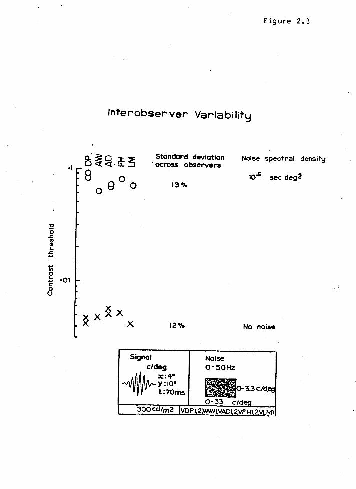
., fl)
~ •Ol c 0 u
Figure 2.3
lnterobser ver Variability
ci·~o ~ OC::t<X·f:J
8 9
o 0 0
Signal
Standard deviation · across observers
13 .,.
~c/d~4o
Y:l0° t:70ms
Noise 0-50Hz
Noise spectral density
10..& sec deg2
No noise
3.3C/d.
0-33 C/d 300 Cd/m2 VOPl,2YAWl,VADl2VFHl2YLMl

CHAPTER 2: THRESHOLDS IN WHITE NOISE Page 57 RESULTS
conditions, only slightly more than the standard deviation of a
si~gle observer. The variations from the mean are consistent for each
observer, but are not obviously correlated between the two conditions. One of
the observers (FH) had never before acted as a psychophysical subject, others
(DP and AW) were very experienced. At the time of this experiment DP had been
observing gratings in noise almost daily for six months. None of the other
observers had ever made observations in noise before. The similar thresholds
of all the observers seems to rule out any large learning effect.
Most of the threshold measurements reported here were made only on DP, the
author. The· 2IFC method was used to avoid effects of criterion changes and
preconceptions on threshold estimat-es. While it would be worthwhile to confirm
some of the findings on other observers, the striking similarities found here
suggest that little difference will be· found between observers.
Effects of noise at two luminances --------Figure 2.4 plots threshold for a 4 c/deg grating as a function of noise
level at two l\IDinances: 330 cd/m2 and 3.3 cd/m2• The noise was white,
two-dimensional, and dynamic. The thresholds at each 1\IDinance are well f1 t by
smooth curves representing proportionality of squared threshold to actual plus
critical spectral density of the noise. Note that the curves converge at high
noise levels, indicating little or no change in calculation efficiency. In the
absence of noise, lowering the l\IDinance by two orders of magnitude increased
threshold in zero noise by a factor of four, but thresholds in high noise were
unaffected •
The equation of the smooth curves is
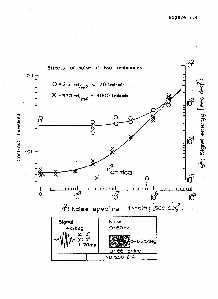
1J 0 .t:. II) G) '-.t:. +'
+' II) 0 '-+' c 0 u
0•1
•01
I 0
Effects of noise at two luminances
0 = 3·3 cd 1m2 ,_ 130 trolands
X = 330 cd1 m2 ,_ 4000 trolands
~ 0
'111111.1 f
2 ncritical
I 4 I I II I ?
I I I I II I
Figure 2. 4
II I 111
1cf n2: Noise spectral densit~ [sec deg
2]
Signal 4c/deg
•
x:2° y: 50 t:70ms
Noise o-50Hz
o- 66 cJd NDP206-214
&6C/deg

CHAPTER 2: THRESHOLDS IN WHITE NOISE RESULTS
2 + n •
lhe f1 tted values of n~ritical are indicated on the abscissa.
Page 58
We have seen that squared threshold is proportional to the sum of the
critical and actual noise levels. Lowering the luminance from 330 to 3.3 cd/m2
increased the critical spectral density, without changing the constant of
proportionality, implying that the calculation efficiency was constant. With
all parameters shown explicitly, our relation becomes
2 (d')2 2 2 s = ~ (ncritical + n ).
d' was 1. 27 throughout, corresponding to 82S correct in the 2IFC task. lhe
fitted curves indicate that the calculation efficiency was .4S at all. noise
levels and at both luminances. lhe critical ~pectral density was 2.3 10-8 sec
deg2 at 330 cd/m2 (approximately 4000 trolands), increasing to 6.5 10-7 sec
deg2 at 3.3 cd/m2 (approximately 130 trolands).
Estimates of transduction efficiency ~ published work
Figures 2.5 and 2.6 show similar data from Nagaraja (1964). Figure 2.5
shows contrast thresholds for a 14.7' diameter disc as a fUnction of noise
level, at three luminances, .034, .34, and 3.4 cd/m2, corresponding
approximately to· .9, 7, and 50 trolands respectively. As before curves
representing proportionality of squared threshold and effective noise level
were fit by eye, and the c~itical spectral density esimates thus obtained are
indicated on the abscissa.
Figure 2.6 shows threshold for three different disc diameters (5.7',
14.7', and 32') as a function of noise level at one luminance (.34 cd/m2 • 7

1
.. ';;) .1 ca .. ~ c 0 0 , 0 .c (I) G)
1: t-
. 01
after Nagara ja (1964)
X • • 034 allm2-. 9 trolands a .. 34 aJ/m2-7 trolands
0· 3.4 al/m~50 trolands
Figure 2. 5
14.7 disc diameter
2 "critical
Io-5 10-4
[sec deg 2)
Noise Spectral Density

(,) .. .., t/1
"' ... .., c 0
(.)
'0 -0 .c (I) Cl) ... .c 1-
Figure 2.6
1~------------------------------------~------~
.1
0
after Nagaraja (1964)
X • 5. 7' diameter disc /). • 14. 7' diameter disc 0 .. 32' diameter disc
• 34 cd/m2 -7 trolands
2 n critical
10-5 10-4
[sec deg 2]
Noise Spectral Density

CHAPTER 2: nfRESHOLDS IN WHITE NOISE RESULTS
Page 59
trolands). Note that the three disc sizes result in virtually identical
2 estimates of ncritical·
Figures 2.7 and 2.8 show results from dot experiments of van Meeteren and
Boogaard (1973) and van Meeteren (1973). Figure 2.7 shows threshold contrast
for a ~.5 c/deg grating, 3°x3° viewed foveally, as a function of noise level,
at three retinal illuminances (.035, .35, and 3.5 trolands). Figure 2.8 shows
similar results for a 2.2 c/deg grating viewed 7° in the nasal field, at five
retinal illuminances (.0013, .013, .13, 1.3, and 13 trolands).
Transduction efficiency versus retinal illuminance
2 Finally, the estimates of ncritical from the preceding graphs (Figures
2.~ through 2.8) were used to calculate the transduction efficiencies which are
plotted in Figure 2.9 as a function of retinal illuminance. The highest of the
transduction efficiency estimates is 2.6S at .0016 troland, 7° nasal field, and
the lowest is .~3S at ~000 trolands. Unlike quantum efficiency estimates;where
sometimes only the values for optimal signals are reported, Figure 2. 9 shows
transduction efficiency for all data sets that could be found which report
thresholds with and without two-dimensional dynamic white noise at the same
luminance. These estimates vary less than tenfold over nearly seven decades of
light level, and a variety of signals.
The sloping dashed line represents the highest quantum efficiencies Barlow
(1962b) found, while the horizontal dashed line represents Barlow's (1977)
lower bound (11S) on the photometric estimate of the fraction of corneal
photons that excite rods.

Figure 2. 7
1~------------------------------------------~
J . • 1 " . i 0 "a j • • ~
.01 0
0
after van Meeteren and Boogaard (1973)
X • • 035 trolands ~ • .35 trolands 0 • 3. 5 trolands
2 "critical
n2 [sec deg 2)
Noise Spectral Density
4.5 c/deg
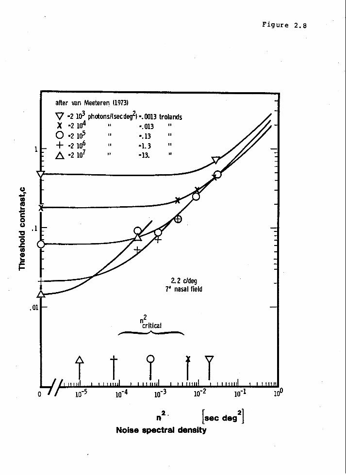
() .. .. fl) «t ... c 0 () , 0 .c fl) Q) ... .c ...
after van Meeteren (1973)
V •2 103 photons/(secdeg2) •. 0013 trolands X •2 104
II ·.013 II
0 •2 1oS II • .13 II
+ •2 106 II •1.3 II
8. •2 107 II •13. II
2 "critical
2. 2 c/deg 7° nasal field
n2
· [sec deg2
]
Noise spectral density
Figure 2. a

10%
1%
TE
.1%
TRANSDUCTION EFFICIENCY
Barlow's (1977) lower bound on the fraction of corneal quanta (507 nm.) ---.--- ---- ------------that excite rods
D ., D ',,
', • • ', ~ ',
Q ~.,...~' ~_, ~,',
"'I' .r ' &or?%', "'~~ ~~ ',,
v~. ~~· ', (.0-6- ~c?/ ', . '
'
D
' ', X • 4 c/deg, this thesis ',
' 0 · discs, 5. 7'- 32', derived from Nagaraja (1964) ', 0 · 4. 5 c/deg, foveal, derived from van Meeteren and Boogaard (1973) • • 2 c/deg, 7° nasal field, derived from van Meeteren (1973)
.001 .01 .1 1 10 100
Trolands
10%
1,
X
.1%
1000 10,000

CHAPTER 2: THRESHOLDS IN WHITE NOISE REVIEW
REVIEW
Thresholds in white noise ---
Page 60
Rose's (1942, 1948) and de Vries's (1943) best-known contribution is now
called the Rose-de Vries law. For Rose, at least, it rested on two
assumptions: (1) that "quantum efficiency of the eye" (i.e. transduction
efficiency) is constant,
TE = constant,
and (2} that threshold occurs at a given "threshold signal-to-noise ratio", k,
at the output of the eye,
k = constant.
We have seen that Rose's k is the effective signal-to-noise ratio, i.e. square
root of the ratio of signal energy, s 2, to effective noise, n2 effective•
k 5 (s/n)effective 2 2 = s/l(n +ncritical>.
So Rose's second assumption is,
(s/n)effective = constant.
If the thresholds all have the same d' , as in the Blackwell ( 1946) data Rose
used, then this assumption implies that the calculation efficiency is constant.
Assuming constant transduction and calculation efficiencies implies a constant
quantum efficiency. The Rose-de VTies law is just the statement that the
quantum efficiency is constant.
Rose tested his assumption that k, the effective signal-to-noise ratio, is
constant at threshold by measuring thresholds for discs on a dot display. He

CHAPTER 2: THRESHOLDS IN WHITE NOISE Page 61 REVIEW
implemented an ideal image intensifier which produced a bright dot for each
detected P"toton. Imaging a test pattern of discs of various areas and
contrasts, Rose found that the product of threshold contrast and disc diameter
was constant, as predicted. This was also true for static P"totograP"ts of the
~!splay. In these experiments Rose found that the effect! ve signal-to-noise
ratio at threshold was 5. By assuming that threshold is always at an effective
signal-to-noise ratio of 5, Rose could estimate the fraction of the corneal
quanta which were transduced by the eye. Rose was the first to compare effects
of photon noise and luminance noise. Rose's paper was seminal for the study of
both phenomena, yet since Rose they have usually been treated as. unrelated.
Sturm and Morgan (1949) applied Rose's (1948) ideas to roentgenoscopy (now
. called fluoroscopy: examination of a patient's x-ray shadow by direct viewing
of a fluorescent screen), and roentgenography (now called radiography: a
photographic plate is placed in contact with the fluorescent screen, and after
developnent the resulting "radiograph" is examined). It was lmown that w1 th
similar x-ray fluxes radiologists could make out much more detail in a
radiograph than by fluoroscopy. Many suspected that this difference was due to
the high luminance at which the radiographs were viewed (approximately 300
cd/m2 ) and the low luminance of the fluoroscopic screen ( .001 to .01 cd/m2 > ~
Apparently it was thought at the time that the visibility of detail on the
fluoroscope would at least equal that in radiographs if the fluoroscope screen
could be made sufficiently bright (by increasing the number of visible photons
emitted per incident x-ray photon). Sturm and Morgan used Rose's fluctuation
theory to show that the greater visibility of detail in the radiographs was
primarily due to the use of film exposure times much longer than our eye's
integration time, so that the radiologist effectively used more of the x-ray
quanta when he viewed the radiograph.

•'
CHAPTER 2: THRESHOLDS IN WHITE NOISE Page 62 REVIEW
Sturm and Morgan made a transparency of an array of discs of graded area
and contrast and held it against the scintillating fluo~oscopic screen. They
determined contrast thresholds for each disc size. They used Rose's estimates
of the "quantum efficiency of the eye" CSS), and "integration time" (.2 sec),
~nd the threshold signal-to-noise ratio (5) to predict the value of the product
c,I(AI), where c is.contrast, A is disc area, and I is screen luminance. The
contrast thresholds for the discs were as predicted, except that the smallest
and largest discs had higher thresholds. This showed
that fluoroscopy was approximately light-limited.
They also, in effect, modulated the x-ray beam by an array of discs, made
a radiograph, and then determined contrast thresholds from the developed
radiograph. Again they used fluctuation theory to predict the product c,t( AI),
where I is now dot nux (i.e. detected x-ray photons per second per screen
area). Again the thresholds were higher than predicted for the smallest and
largest discs. This confirmed that radiography was approximately
x-ray-exposure limited.
Their most important contribution was the idea that thresholds for dot
images would be limited by the total noise whose power equals the sliD of the
power at the retina of the photon noise and the dot noise, and that one or the
other would usually be sufficiently greater to make the smaller one negligible.
"Now these sources of fluctuation in the roentgenoscopic screen process are essentially independent of one another • • • Therefore, it may easily be shown by statistical theory that the average total fluctuation at the termination of the roentgenoscopic process when the nerve impulses are finally transmitted from the retina to the brain is given by the equation
where s 1,s2, • • • ,sn are the values at the retina of the various average fluctuations introduced at the various phases of the roentgenoscopic process."
CHAPTER 2: THRESHOLDS IN WHITE NOISE Page 63 REVIEW
The practical conclusion of their paper was that increasing the brightness
of the nuoroscopic screen (without increasing the detected x-ray flux) would
only reduce the photon noise (i.e. inverse of effective photon nux) which was
not much larger than the dot noise (i.e. inverse of detected x-ray photon
flux), so that even a much brighter screen could not be as useful as the
radiographs.
Schade (1951, 1952, 1953, 1955) did signal-to-noise ratio analyses of
photographic and television systems. He later said (Schade 1964),
"I was told by Dr. Gardner of NBS [National &lreau of Standards] at one of those lectures, I believe it was in 1952, that the great interest aroused by these lectures in the optical and photographic professions was due to the fact that I demonstrated for the first time that sine-wave response and noise in televison and photographic systems could be evaluated on a unified basis and measured with practical instruments, yielding objective data on the performance of practical system elements and canplete systems. Without such instrumentation and numerical evidence, there would have been little interest in the mathematical theory."
Coltman (1954) used an ideal image intensifier to image a ten-bar pattern
(i.e. 10 cycles of a square ~ve) of adjustable contrast. Squared threshold .
(50S "seen") was approximately proportional to the recipro~al of speck flux
(i.e. proportional to spectral density) over two orders of magnitude.
Green, Wolf, and White (1959) used a computer to generate still
photographs made up of a matrix of black and white dots. Each dot had a prior
probability of being White (versus black); patterns were created by modulating
the prior probabilities. Using this static dot display they presented 4 cycles
of a square wave (with one probability over the lighter bars, and another,
lower, probability over the darker bars). They measured the detectability of
these square waves by asking the observer to state whether the bars were
horizontal or vertical. They determined the signal contrast 21 required for
CHAPTEJl 2: THRESHOLDS IN WHITE NOISE REVIEW
75J-correct responses by the observer.
Page 64
"To a first approximation the threshold is directly proportional to the standard deviation of the dot-density distributions. The threshold of the ideal statistical detector has the same properties as the thresholds obtained • • • , but is much lower. Thus we may say that for a fixed pattern, and a fixed exposure, our observers behave like the ideal detector, except for sensitivity."
In other words,_the efficiency was constant.
Coltman and Anderson (1960) measured contrast threshold (50S "yes") for a
sinusoidal grating on a television display with added two-dimensional dynamic
white noise. They found an initial fall in threshold over the first five
trials of 3 dB (i.e. to .7 of the initial value). This; probably reflects a
lowering of the criterion for "yes" by the observer. "The effect of changing
viewing distance over a range of 30:1 is hardly outside the experimental error
in determining the threshold." Since changing the viewing dist~nce doesn't -
change the signal-to-noise ratio, s/n (because s2 and n2 are reduced equally by
increasing the viewing distance), this implies a constant signal-to-noise ratio
at threshold for a 30: 1 range of spatial frequencies. And so they concluded,
"It is found both theoretically [with fluctuation theory] and experimentally that the masking effect of white noise depends only on the noise power per unit bandwidth, and is independent of the upper frequency limit of the noise spectrum, provided that this. exceeds the frequency limit set by the eye."
Griffiths and Nagaraja (1963) and Nagaraja (1964) reported thresholds (50S
correct, after correct~on for guessing) for bright discs masked by white noise
(dynamic , and two dimensional) • The target was a bright disc , 6' , 15 ' , or 32'
in diameter, which appeared for 8 seconds in any of 8 possible locations.
Nagaraja found that the square of the threshold contrast was proportional
21 Their definition of threshold wasn't contrast; it was the difference in prior probability between the white and black bars, but, for any given mean luminance the two measures are proportional and the meaning of their quoted ~nn~lu~i nn i ~ un~h~naM _
CHAPTER 2: THRESHOLDS IN WHITE NOISE Page 65 REVIEW
to the sum of the spectral density of the noise plus a constant, the "internal
noise" (see Figures 2.5 and 2.6). This is evidence that calculation efficiency
is independent of noise level. The "internal noise". was equal, within
experimental error, for the three targets (see Figure 2.6). The "internal
~oise" was higher at lower luminances, and he showed that the "internal noise"
was of similar magnitude to that expected from fluctuations in the number of
quantal absorptions in the retina at the three luminances tested (.03, .3, and
3 cd/m2), assuming .51 to 11 absorption.
Nagaraja (1964) calculated that his "intrinsic noise" might be due to
photon noise, taking ..tlat he felt was a reasonable guess as to the fraction
usefully absorbed. It is more interesting to do the opposite: calculate what
· fraction of the photons would have to be usefully absorbed to account for his
"intrinsic noise", i.e. transduction efficiency. I calculate 22 Nagaraja's
transduction efficiencies to be 0. 81, 0. 51, and 0. 61 at estimated retinal
illuminances'of .9, 7, and 50 trolands, respectively. They are plotted on
Figure 2.9. The differences between these transduction efficiencies are not
significant because the pupil diameters were not measured, but only estimated.
later from standard tables, and thus the pupil areas may be in error by a
factor of two in either direction (e.g. see wyzecki and Stiles p. 213).
Griffiths and Nagaraj a ( 1963) compared the human performance data with
ideal performance. They present graphs of proportion correct in the
eight-alternative forced choice task as a function of the signal-to-noise
22 Pupil sizes were not reported so the retinal illuminance in trolands was estimated directly from the luminance using a standard graph (Wfzecki and Stiles 1967, p. 214). Since the observers used both eyes the to.tal photon nux Jphotons was twice that for one eye.

CHAPTER 2: THRESHOLDS IN WHITE NOISE REVIEW
Page 66
ratio. They reported that the human observer required a signal-to-noise ratio
almost three 2 ' times greater than the ideal. For an 8 second presentation
(8AFC) efficiencies (in luminance noise) calculated from their data are 4S for
a 5.7' diameter disc, 7S for 9.8', 6S for 14.7', 11S for 21', and 8S for 32'.
For brief presentation (2AFC) of the 21' disc the highest efficiency was 13S
for a 320 millisecond duration.
Schade (1964) had observers identify the smallest visible bar triplet on a
US Air Force 3-bar test object in the presence of a range of static white noise
levels. He found the signal-to-noise ratio of these thresholds to be nearly
constant over a wide range of noise levels.
Chambers and Courtney-Pratt (1969) asked observers to determine the
location of a randomly-located patch of higher dot density in a background of
randomly-located black dots on a white background. The patch could be anywhere
on the square background. They compared the observers' performance with that
of fluctuation theory, and, for good measure, a computer that acted as an ideal
observer. The computer's performance was always very close to the theoretical
prediction. Threshold was taken to be the number of extra dots in the signal
patch required for 50S correct identification of location.
"The computer when instructed to pic~ the signal location on the basis of a highest dot count, required about ~ as much signal as a human observer for correct detection on 50S of the plots."
This implies a constant efficiency of (~)2:44S.
~llehn and Roehrig (1970) displayed sinusoidal gratings with added noise
on a television display. Some peculiarities in their results indicate that the
modulation transfer function of the displaY, was far from flat 2 ', but this would
2 3 The reader desiring to check this calculation should be aware of their unconventional definition of "dB, as 10 log c" (Nagaraja, 1964), whereas dB conventionally represent 20 log c.

CHAPTER 2: THRESHOLDS IN WHITE NOISE REVIEW
Page 67
not affect the results of interest to us now. They plotted threshold contrast,
c, versus rms noise contrast for four spatial frequencies and fit each by a
curve
where crms was the rms contrast of the white noise added to the signal. As
discussed in Appendix 1, for a given bandwidth, the spectral density, n2, of
white noise is proportional to its contrast power, c~s· They only say that,
"This fit implies an interpretation of [k] as the internal noise of the visual
channel." The dependence of k on the spatial frequency of the signal is
confounded by the MTF problem alluded to above.
Goodenough, Rossman, and Lusted (1972)·carefully studied the detectability
of a small spot of light "projected onto uniformly exposed radiographic samples
. i exhibiting the coarse fluctuations in density, called radiographic mottle,
which constitute a source of noise in the detection process." They asked
2 ' In their figure 11 they plot threshold contrasts for three spatial frequencies as a function of viewing distance. In effect this varied the screen size from 2 to 60 degrees. For 2 c/deg increasing the screen size by a factor of 4 increased sensitivity by a factor of 4. For 6 c/deg increasing screen size first increased, then decreased sensitivity. For 15 c/deg increasing screen size by a factor of 3 decreased sensitivity by a factor of 3. Effects of screen size have been reported by others, but they are always of the same form: a steep reduction in sensitivity when less than 4 periods are displayed (e.g. Campbell and Robson 1968), and a very gradual increase (a factor of 1.2 per octave) in sensitivity as more periods are displayed (Robson in Mostafavi and Sakrison 1976, Robson and Graham 1981). The contradiction may be resolved by supposing that the modulation transfer function (MTF) of the tv display used by Pollehn and Roehrig was far from flat. To test this theory I replotted their three graphs of sensitivity versus observing distance all on one graph of sensitivity versus number of bars across the screen. The three curves then differed only by a scale factor in sensitivity. This graph indicated that the MTF of the display had a full bandwidth of 4 octaves at half height, centered at about 80 cycles/screen. They state that, "The bandwidth of the apparatus was 8.5 MHz (3 dB point)." However, the MTF I calculated from their data has already fallen a factor of 4 (i.e. 12 dB) at 6.5 MHz. Since all the noise spectra were measured only at the input of the display, we cannot be sure of the spectra of the displayed patterns. this prevents quantitative
·interpretation of all of their results that involve more than one spatial frequency or viewing distance.

CHAPTER 2: THRESHOLDS IN WHITE NOISE REVIEW
Page 68
observers to rate (on a five point scale) the likelihood that the spot was
present. The spot could be anywhere on the radiograph, estimated by the
authors to include about 800 non-overlapping positions. Detectability of the
signal on one noise background ("resulting from a fast speed screen - medium
~peed film combination") was much higher than on another ("resulting from a
medium speed screen - fast speed tllm combination") which had approximately
twice the spectral density and bandwidth as the first.
Strom eyer and Julesz ( 1972) measured threshold by the method-of-adjustment
for a sinusoidal grating in one-dimensional dynamic white noise (white over
0-30Hz 25 and 0-54 c/deg). For two observers for three spatial frequencies, the
square of the threshold was proportional to the spectral density21 of the noise
over the two orders of magnitude tested.
Rosell and Willson (1973) measured thresholds (32S correct, 4AFC) for
bright rectangles presented for 10 seconds in dynamic two-dimensional white
noise. With some assumptions 27 their results indicate that at a constant
luminance and noise spectral density and threshold criterion, the observer's
calculation efficiency seems to be constant for rectangles in the range .1°x.1°
to • 5°x4°' and about fourfold lower for rectangles with larger minimum
25 Their 60 Hz frame rate implies that the noise spectrum is white only up to the Nyquist frequency, 30 Hz. This issue was discussed ,at the beginning of this chapter.
2 ' Stromeyer and Julesz did not report2the spectral density, but it is easily
calculated as the ratio of the power crms and the (double-sided) bandwidth, which were both reported.
27 Results are reported in terms of the "signal-to-noise ratio" at threshold, but they do not clearly define the term. In one respect their quantity is certainly suspect: their calculations reduce the signal duration to .1 seconds, to account for the "integration time" of the observer's eye.

CHAPTER 2: THRESHOLDS IN WHITE NOISE REVIEW
Page 69
Image intensifiers were a natural application for fluctuation theory.
However image intensifiers for field use have compromised a variety of
desirable qualities, presumably in order to maximize portability and quantum
efficiency. In particular the imaging properties are far from uniform over the
field. Therefore experiments designed to study vision have used apparatus
similar to that used by Rose (1948), a flying spot scanner linked to a
kinescope (i.e. a closed-circuit television monitor). Quantum efficiencies
tend to be low but plenty of light is available. Such a device will be called
an ideal image·intensifier, to distinguish it from the commercial image
intensifiers designed for field use.
In a review of his earlier work, Rose (1957) said,
"There are other more direct ways of measuring quantum efficiencies. These involve a simple side-by-side comparison of the human eye with other picture-recording devices of known quantum efficiency. For example, let an observer and a television camera view the same test pattern side-by-side. The observer need then only compare what he sees of the test pattern with what he sees reproduced on the television monitor to decide whether his quantum efficiency is greater or less than that of the television camera. The great virtue of this method is that one is not dependent on a knowledge of the storage time of the eye or of the threshold signal-to-noise ratio. Since the same observer compares the original and reproduced patterns, the same storage time and threshold signal-to-noise ratios are effective and their influence on the comparison cancels out."
Rose's estimate of the "quantum efficiency of the primary photo process"
(i.e. the transduction effi,ciency) is the ratio of the ntaber of dots for
threshold with the image intensifier (at a high luminance) divided by the
number of corneal photons for the same threshold contrast with unaided vision
(at a much lower luminance),
TE = Jdots(high luminance)/Jphotons(low luminance).

CHAPTER 2: THRESHOLDS IN WHITE NOISE REVIEW
Page 70
This operational definition of the "quantum efficiency of the eye" differs
slightly from Rose's (1948) earlier one, but insignificantly for our current
purposes. 21 Rose (1957) suggested we calculate the "quantum efficiency of the
eye" from the noise level at a high luminance that produces the same threshold
¢ontrast as zero noise at a lower luminance. Let us .call that the
!so-threshold method. We have based estimates of transduction efficiency on
two different thresholds at the same luminance. Let us call it the
!so-luminance method. Both methods depend on the calculation efficiency being
equal for the two measurements. The !so-luminance method requires that the
calculation efficiency be independent of the noise level, which available
evidence indicates is true. The !so-threshold method requires the calculation
efficiency be independent of luminance, but we will see evidence that this is
often false. Nagaraja (1964) used the !so-luminance method, but most of the
21 We have seen that the 1948 definition is equivalent to the transduction efficiency. Rose's (1957) new technique is to measure how much luminance noise at a high luminance equates the photon noise at the low luminance. Because of this pure substitution of· luminance noise for photon noise their ratio will not be affected by any component of the observer's equivalent noise that is independent of luminance. Thus this second definition of "quantum efficiency of the eye" would seem to be a purer measure of the efficacy with which photons are utilized. However, the method is impractical because few, if any, devices can be assumed to have a constant calculation efficiency over the wide range of luminances required.
If it is desired to leave out the luminance-independent part of the observer's equival~nt noise it would be better to determine what that component is (by measuring nQritical at many luminances) and subtracting it out before dividing into the pnoton noise. This might be called a "corrected transduction efficiency", "CTE",
2 nphotons< at L)
CTE = 2 2 ncritical(at L)- ncritical(at 100L)
2 . In fact, over the ranges which n it~ 1 has been measured it falls so quickly with increase in luminance that fhe g8rrected transduction efficiency" would not differ significantly from the standard transduction efficiency.
CHAPTER 2: THRESHOLDS IN WHITE NOISE REVIEW
Page 71
published estimates of transduction efficiency were made by the !so-threshold
method and cannot be relied on.
Some experiments have been reported which used commercial image
intensifiers (e.g. Ruedy in Jones 1959; Beurle 1969, van Meeteren, Vos and
Boogaard 1971, Rosell, Svenson, and Willson 1972, and Engstrom 1974). Most of
these were rough confirmation of the applicability of fluctuation theory to
visibility of patterns in dot noise, but several went on to estimate
transduction efficiency by the !so-threshold method. Jones (1959) reported,
"In a February 13, 1959, letter, Dr.~.E.Ruedy reports2
an experiment in which a target at a luminance of 10- ft-L [.003 cd/m ] was viewed directly, and also via a television system using an intensifier orthicon. Nine observers were used. It was found that when the detective quantum efficiency of the television system was ten percent, the detectability of the target was roughly the same by direct viewing and via the television system."
In a similar experiment using 533 nm monochromatic light, Engstrom (1974)
reported transduction efficiencies between 1J and 4% (at 533 nm) from about .01
to 1 troland, except for one observer (the youngest at age 30) whose
tranduction efficiency estimates were unaccountably nearly tenfold lower, in
the range .2% to .5%.
van Meeteren and Boogaard (1973) built an ideal image intensifier like
that used by Rose ( 1948); .each detected photon produced a small brief speck on
the display. They used it to image sinusoidal gratings. They defined
threshold as the contrast required for 75% correct identification of the
orientation of the grating which was always vertical or horizontal. At high
speck energies (i.e. many photons per speck) threshold was independent of speck
energy29 • Using high-energy specks they confirmed earlier reports that
contrast sensitivity was proportional to the square root of speck flux. That
is, that squared contrast threshold was proportional to reciprocal speck flux,
CHAPTER 2: THRESHOLDS IN WHITE NOISE REVIEW
and thus proportional to spectral density,
Page 72
They also reported measurements of contrast sensitivity for continuous gratings
(i.e. not made up of specks) under otherwise identical conditions. They used
Rose's (1957) !so-threshold method to calculate the transduction efficiency,
which they called the fraction of quanta "effectively absorbed". Presuming
that specks each. containing 500 photons were fully effective, they determined
the speck flux, Jdots• required to give the same threshold as obtained with a
continuous grating at a lower luninance with photon nux Jphotons•
Jdot8 /Jphotons was 1~ from 3.5 down to .35 trolands, and fell to .4~ at .035
trolands.
Figure 2.7 shows their data replotted as threshold contrast versus noise
spectral density. Each symbol represents data from one luninance, .035, .35,
and 3.5 trolands. The data at each luninance are reasonably well f1t by
proportionality of squared contrast to effective noise level, except that for
the two higher luminances threshold is higher without noise than with the
lowest noise level. This is surprising. van Meeteren and Boogaard said,
"The conclusion must be, that the particular stimulation with clusters of photons is more effective than the normal stimulation in this case."
Since the discrepancy is only a factor of 1.5, an alternate explanation is
suggested by the fact that the zero-noise thresholds were collected as part of
a previous study (van Meeteren and Vos 1972), and Were not remeasured
presumably because it was not feasable to produce zero-noise images with the
21 Their expectation was that with a sufficient nunber of photons per speck the observer would be able to utilize virtually every speck. This was confirmed; contrast sensitivity (i.e. 1/threshold) rose as the number of photons per speck (i.e. speck energy) was increased until a critical speck energy, beyond which threshold was constant. They found that the critical speck energy was not a ,.,....,a • .,..,.. ...., .... A ........... A.-..A """ +-"-'"" 1 •-" ... """""'""
CHAPTER 2: THRESHOLDS IN WHITE NOISE Page 73 REVIEW
arrangement required for dot display.
2 The estimates of ncritical were used to calculate transduction
efficiencies (by the !so-luminance method) which are plotted on Figure 2.9 as
open squares. The transduction efficiencies, 2.1S, 3S, and 1.8S at .035, .35,
and 3.5 trolands, respectively, are higher'' and more constant than van
Meeteren and Boogaard's estimates (.4S, 1S, and 1.2S) calculated by the method
~ of !so-threshold from the same data. As we noted earlier the !so-threshold
estimates of transduction efficiency depend on the assumption that the
calculation efficiency is independent of luminance. Figure 2.7 shows that the
calculation efficiency for the 4.5 c/deg grating is virtually the same at .35
and 3.5 trolands, but is much lower (i.e. the high-noise threshold is higher)
at .035 trolands. These data were all from a 3°x3° grating centered on the
fovea. They showed that thresholds for frequencies in the range 2 to 15 c/deg
were all raised in the same proportion in the speck image condition, relative
to a noise-free condition, implying that the transduction efficiency is the
same for 2 to 15 c/deg at these luminances.
In his thesis, van Meeteren (1973) includes the data of van Meeteren and
Boogaard (1973) and similar data for a 2.2 c/deg grating at 7° nasal field as
well. Figure 2.8 shows his data, replotted as threshold contrast versus noise
3 0 A small part of the reason my estimates are higher is that I assumed
1 lumen= 4.1 1015 quanta (at 555 nm)/sec, 5
(Wyzecki and Stiles 1967) while van Meeteren and Boogaard seem ,to have assumed, for no apparent reason, that
1 lumen = 5.3 1015 quanta/sec.
I arrived at their figure2by comparing the abscissas, one in cd/m2 and the
other in photons/(sec min of arc), on otherwise identical graphs of zero-noise contrast sensitivity.

CHAPTER 2: THRESHOLDS IN WHITE NOISE REVIEW
Page 74
level, at five luminances (.0013, .013, .13, 1.3, and 13 trolands). The data
are well f1t by curves representing proportionality of squared contrast and
effective noise level. The calculation efficiency is constant for the three
middle light levels, and slightly lower (i.e. the high-noise threshold is
~igher) at the lowest (.0013 trolands) and highest (13 troland) light levels.
It is to be expected that sensitivity (i.e. reciprocal of threshold) at a given
speck flux would increase initially if speck energy (i.e. photons per speck) is
increased. van Heeter en found that it
"tends to decrease again when the speck-intensity is made very high, as was predicted by Beurle (1969) and demonstrated also by Hodgaon 11 ."
Beurle's prediction was based on consideration of changes in the eye's
integration time and area with luminance, which is a possible explanation for
the changes in calculation efficiency.
Again the estimates of n2 iti 1 were used to calculate transduction · .. cr ca
efficiencies which are plotted in figure 2.9. The transduction ~fficiency is
maximum, 2.6S, at .0016 troland; it falls gradually from .9S to .5S from .016
to 16 trolands. These transduction efficiency estimates seem very low. They
are lower than the foveal transduction efficiencies at light levels (.016 to
1.6 trolands) which should favor rods over cones, and thus the periphery over
the fovea. This may be due to my assuming that
1 lumen= 4.1x1o15 quanta (555 nm)/sec
which is, of course, inappropriate at these scotopic luminances; however, van
Meeteren reported the light level only as photopic trolands, so there is no
11 see Hodgson (1972).

CHAPTER 2: THRESHOLDS IN WHITE NOISE Page 75 REVIEW
obvious remedy. Given these uncertainti~s over photon fluxes there may be no
significant difference between the approximately .4S transduction efficiency
estimates from my data, the approximately .6S estimates from Nagaraja's data,
and the approximately 2S transduction efficiency estimates from van Meeteren
~nd Boogaard' s data.
This agreement is particularly interesting since van Meeteren and Boogaard
used sinusoidal gratings in speck noise, while Nagaraj a used discs in
continuous white noise, and I used gratings in continuous noise. All the
transduction efficiencies on Figure 2. 9 are within • 4S to 3S. This includes
discs of 5.7' to 32' in diameter, gratings of 2 to 15 c/deg, foveal and 7°
nasal field viewing, and retinal illuminances of .0016 to 4000 trolands. The
small variation of transduction efficiency may be contrasted with the enormous
variation of quantum efficiency found over a comparable range. As shown in
Figure 2.9, Barlow's optimal quantum efficiency (at 15° nasal field) fell two -;;. -
dec~des over the luminance range of van Meeteren's 7° nasal field data. For
van Meeteren and Boogaard's data for 4.5 c/deg (Figure 2.7), the calculation
efficiency changed fourfold while the transduction efficiency was approximately
constant, indicating a fourfold variation of-quantum efficiency where there is
no change in transduction efficiency. van Meeteren and Boogaa~d showed that
thresholds on their dot display were raised by the same proportion for all
spatial frequencies from 2 to 15 c/deg, implying a constant transduction
efficiency, but the signal energies at threshold indicate that quantum
efficiency (and calculation efficiency) tor 2 c/deg is 44 times higher than for
15 c/deg.
By its definition the transduction efficiency must exceed the quantum
efficiency for the same signal. At the fovea, van Meeteren and Boogaard (1973)
CHAPTER 2: THRESHOLDS IN WHITE NOISE Page 76 REVIEW
showed that gratings of 2 to 15 c/deg give the same transduction efficiency, so
we might suppose a similar constancy in the periphery in order to allow a
comparison with Barlow's (1962b) determinations of quantum efficiency. Barlow
reported. quantum efficiency for optimized targets at 15° nasal t.leld. This is
~hown on Figw-~ 2. 9 as a dashed line with negative slope. However van
Heeter en's data are from 7° nasal t.leld. At 7° nasal t.leld Barlow reported
only the quantum efficiency in the dark. Barlow's quantum efficiency in the
dark ~s higher at 15° nasal t.leld (5S) than at 7° nasal t.leld. Perhaps the
transduction efficiency too is higher at 15° than at 7° nasal t.leld.
Barlow (1978) reported efficiencies for detecting discs of various
diameters and dwoations on a speck display. Barlow reported as efficiency for
a 1 second 0.69° flash, which agrees well with Griffiths and Nagaraja's (1963)
report of 6S efficiency for a 12' diameter disc exposed for 640 milliseconds on
two-dimensional dynamic lili te noise. However with brief signals Barlow
obtained much higher efficiencies than Griffiths and Nagaraj a did. thi~ is
probably because Griffiths and Nagaraja kept the noise on continuously, while
Barlow displayed specks on his display only during signal presentation.
Barlow's brief signals resulted in a brief display, in effect, a glimpse of a
static display. Elsewhere in the same paper Barlow showed that displaying a
static display as long as the observer wishes instead of only 112 milliseconds
improves his efficiency only "marginally".
With a static dot display (i.e. the prior probability of dots was higher in
the target area, but the dots were otherwise randomly located) Barlow attempted
a parametric study of the effects on detective efficiency of average backgrotmd
dot density, but this was confounded by changes in average luminance, as the
luminous energy of each dot was kept constant. Nevertheless several of his

CHAPTER 2: THRESHOLDS IN WHITE NOISE Page 77 REVIEW
results are noteworthy. When the background ~ontained an average of only 8
dots, efficiency was 100S. This will be discussed shortly. Except for this
unique condition, efficiencies were never significantly above 50S. Efficiency
was about 50S for a 15' by 15' square target.
Cheaters and Hay (1979a) measured threshold for detection of a static disc
of light added to static two-dimensional noise. The discs were from • 5' to 2°
in diameter. The background was enlarged }:ilotographic grain, flat in spectrt.lll
up to 10 c/deg. Threshold was determined by increasing the signal contrast in
steps until the subject said "yes". Catch trials measured the false positive
rate (2.6S without noise, 4S with noise).
The contrast sensitivity function (i.e. reciprocal of threshold, as a
function of disc diameter) was similarly shaped for the two observers with and
without noise backgrounds. Squared threshold was proportional to the sum of
the spectral density and a fitted constant. The fitted constant was
interpreted as "intrinsic noise".
The lowest threshold signal-to-noise ratio was obtained for discs between
15' and 30' in diameter. Threshold rose for smaller and larger discs.
Estimating d' in their experiments to be 1.9511 , and calculating the s/n to be
2.4 from their signal and noise measurements, the detective efficiency for the
15' to 30' discs was (d')2/Cs/n) 2.66S. Because my estimate of d' is unreliable
we can only conclude that the efficiency is not in disagreement with the
approximately 50S value found by Barlow using briefly presented signal and
11 They did not do a proper yes-no experiment, but they did state that "in a preliminary series of measurements no systematic difference was found between the 50S threshold obtained by the conventional [yes-no] method and by the modified version." Since they also reported the false-alarm rate, it was possible to estimate d' as the difference between the normal deviates corresponding to the 50S hit rate and the 2.6S false-alarm rate.· Thus d' = z(50S)-z(2.6S) = 1.95.

CHAPTER 2: THRESHOLDS IN WHITE NOISE REVIEW
noise.
Page 78
Burgess, Humphrey, and Wagner (1979) measured method-of-limits thresholds
for a bar optically superimposed on a background of static, two-dimensional
noise,
"the results are fitted by the expression
2 2 ctN = Cto + kN
where cto is the contrast threshold for no external noise, ctN is the threshold for • • • external noise power N, and k is a constant."
Dots and specks versus continuous noise
Modulating dot rates is conceptually different from adding a continuous
signal to a continuous noisy background, yet we have seen both exper~ments
yield similar results when analyzed in terms of the squared threshold contrast
of signal and the spectral density of the noise.
Mezrich (1979) provides some support for this view that dots are not
special. Up to now we have only considered white dots on a black background.
Mezrich showed that easily visible modulations become invisible if the contrast
is reversed so that the dots are black on a white background. He noted that
the (luminance) contrast of the expected signal was lower with the 1 black dots.
At a minimum these demonstrations show that black and white dots are not
treated equally. Mezrich's approach merits quantitative assessment.
There is one respect in which the dot and speck displays seem to be
special. Hirst, Beurle, Beverly, and Poole (1979) reported that at very low
speck fluxes (less than 260 specks per deg2sec) observers' contrast thresholds
are independent of speck flux and are much lower (i.e. more efficient) than
predicted by extrapolation from higher speck fluxes. Barlow (1978) showed that

CHAPTER 2: ,THRESHOLDS IN WHITE NOISE REVIEW
Page 79
observers detect targets on backgrounds.with a mean of 8 dots with 100S
efficiency, whereas efficiency was only 50S for 18 to 200 mean background dots.
Both papers suggested that the subjects might be "subitizing" (rapidly
perceiving the number of a small group of objects) at the lower dot rates. We
can accurately identify the number of randomly arranged dots in a briefly
presented image containing up to about 4 or 5 randomly arranged dots ( Jevons
1871, Kaufman, Lord, Reese, and Volkmann 1949). Jevons (1871) showed this by
repeatedly throwing beans in a cup, glancing inside, and recording both an
estimate and then the actual count. To accurately identify larger numbers we
require more time and some method (e.g. eye fixations) to keep track of which
dots have already been counted; Atkinson, Campbell, and Francis (1976) reported
that,
"the limit of 4 is [still] found if the stimulus is a bright afterimage lasting for approximately 60 seconds."
Barlow (1978) described the strategies of the observers for dot displays,
"If the number was under 7, it could be counted even in the brief exposure used in this experiment (Jevons 1871) ••• As the number increases one makes a 'numerosity judgement,' and it is the inaccuracy of this which causes efficiency to drop. At still higher numbers we thought that it was the texture, dot density, or average dot separation ••• and above this again we thought subjectively that the mean brightness
gave the best cue."
However subitizing could not account for Barlow's data. Kaufman defined
subi tizing as the rapid perception of the number of 6 or fewer items, yet ·
Barlow reported a 100S detective efficiency on a background with a mean of 8
dots. To attain the measured reliability (d'=1) the observer must have used a
criterion of about 8+18=11 dots with few errors. This is much larger than the
4, 5, or perhaps 6, item limit which past authors have found for rapid,
accurate assessment of numerosity, i.e. subitizing. Although estimation of
CHAPTER 2: THRESHOLDS IN WHITE NOISE Page 80 REVIEW
more than 6 dots is inaccurate and has a longer reaction time, it would be
accurate enough for the 11 item criterion implied by Barlow's result. Jevons's
(1871) contingency table for reported versus. actual bean counts indicates his
reports had a standard deviation of about 1 when the actual count was 11. A
dot display with a mean of 8 would have a variance of 8. The observer 1 s
responses would reflect the sum of the variances 8+1 = 9. Thus 8/9 = 89~ of
the variance underlying the observer 1 s response would be due to the variance of
the number of a,ctually displayed, i.e. the efficiency would have been 89~.
Barlow's 100S reported efficiency was not significantly different from 89S. To
see how far this may be extended consider a 50 dot criterion. Jevons reported
that "the average error of estimation • • • is simply proportional to the
excess of the real number over ~·" so extrapolating to 50 we estimate the
standard deviation to be
(50-~)/(11~) = 7.
The variance of the stimulus would be 50, for an efficiency of
50/(50+72> = 51S. Barlow found "there is a range from 18 to 200 [mean
background dots] where performance is about 50S." Thus Barlow's efficiencies
for up to at least 50 background dots may be the result of numerosity
estimation by the observer, but for parsimony we should remember that the
constant efficiency, and thus a constant threshold signal-to-noise ratio also
occur when the signal and noise are continuous, rather than made up of discrete
items.
Hirst et al.'s suggestion of subitizing is more tenable 33 , but estimation
may be the correct explanation there too.
For backgrounds of 25 dots, Burgess and Barlow (1981) have recently shown
CHAPTER 2: THRESHOLDS IN WHITE NOISE .< Page 81 REVIEW
that detection was not affected by approximately doubling the noise spectral 'j'·;r·
density in a way that left dot density constant:
"It is possible that there are cells in the visual system that respond to the total luminous flux emanating from the dots in one hemifield, and that estimation of dot number is based on the responses of such cells. If this were the case the accuracy of estimation would be seriously perturbed by brightening randomly selected dots in each hemifield. the number of dots was judged equally well Y'leri some were dim and some 5 times more intense as when they were all at the some 1 uminance."
Yet, in the same paper, Burgess and Barlow also report the effect of
blurring the dot display. The observer viewed the display "through a diffusing
screen placed at various distances from the oscilloscope screen." There was
"little effect" even when the line spread function was as wide (at half height)
as the entire display. The dot density was high relative to the (two-sided)
bandwidth of the diffusing screen 2x1 x 2x1/screen, so that, with respect to
the diffusing screen the display noise was white, and its Poisson origin would
have been undetectable.
All together these data suggest that we adopt especially efficient I
strategies for static dot displays with less than perhaps 50 dots and dynamic
dot displays with less than 260 dots/deg2sec. At higher densities the discrete
ss Suppose that observers can use their subitizing ability to test whether or . not a certain area and duration of the display contains more than 5 specks.
Presumably the duration would correspond to the 100 msec or so apparent integration by the eye. Further suppose that the observer's criterion is (at least) two standard deviations above the mean (Hirst et al. measured threshold by the method of limits). Then the mean number of dots in the area-duration cannot exceed 2.1, with standard deviation {(2.1) = 1.45. This corresponds to a contrast of 150~, i.e. (criterion-mean)/mean. (Hirst et al. defined contrast of their discs as ~LIL, which can exceed 100~.) The hypothesized subitizer would be an ideal detector (i.e. 100~ efficient) for targets with 5 or fewer specks (signal plus background). If there are more than 5 specks it would count over a smaller area-duration containing 5 specks so its contrast threshold will be constant at about 150S. In fact the thresholds in question were constant at about 100~. lower than predicted for a subi tizer. In view of the speculative nature of this analysis it would appear that subitizing is a possible, if not convincing explanation of Hirst et al.'s data at low speck rates.

CHAPTER 2: THRESHOLDS IN. WHITE NOISE REVIEW
Page 82
nature of these displays does not seem to affect detection; threshold seems to
depend only on the expected signal and the spectrum of the noise.
CHAPTER 2: THRESHOLDS IN WHITE NOISE CONCLUSIONS
CONCLUSIONS
Page 83
Contrast thresholds in white noise have been found to obey the relation
C2 « n2 2 critical + n •
Dot experiments deviate from this relation only at dot nuxes and densities
below that required for the assumption that the noise is white for the channel,
and far below that required for the observer. On that basis it has been
suggested that n~ritical is an estimate of the observer's equivalent input
noise. The ratio of the photon noise to the critical spectral dens! ty has been
called the transduction efficiency.
Since the observer acts in every way as though the cri.tical spectral
density were a luminance noise at his visual f1el~, it has been suggested that
the sum of that and any actual luminance noise be called the effective noise.
Efficiency with respect to the effective noise has been called calculation
efficiency. It has been found that the calculation efficiency is independent
f of noise level.
to Perhaps the important contribution of this chapter has been~show that the
quantum efficiency is the product of the transduction efficiency and the
calculation effici~ncy. It is known that quantum efficiency depends strongly
on parameters of the signal (Barlow 1958, Jones 1959). All the estimates of
transduction efficiency that can be made (by the iso-luminance method) are
between .41 and 31. The conditions span nearly 7 decades of retinal
illuminance, foveal and 7° nasal f1eld viewing, and a wide range of patterns.
This indicates that the violations of the Rose-de Vries law are due almost
entirely to the dependence of calculation efficiency on signal and luminance.

CHAPTER 2: THRESHOLDS IN WHITE NOISE Page 84 CONCLUSIONS
The following chapters will include a few more considerations of the
observer's equivalent noise, but are primarily concerned with calculation
efficiency.
Transduction efficiency, like quantum efficiency, can be measured for any
device, not just human vision. In photography it might help sort out different
causes of inefficiency in the formation of an image. It seems particularly
appropriate for recordings ~om visually-responsive cells, such as
photoreceptors, retinal ganglion cells, and cells in the visual cortex.
Initially it would be desirable to measure the contrast threshold in the
presence of two-dimensional dynamic 'White noise to determine whether the
relation
holds, supporting the interpretation of n~ritical as the cell's equivalent
noise at the visual f1eld, and cont.lrming constancy of calculation efficiency.
If that were found often enough to be assumed then the critical spectral
density could be calculated ~om the contrast thresholds· at any two noise
levels, preferably zero noise and a high noise level, sufficient to raise the
squared threshold by a factor of 2 or more. Any threshold criterion may be
used.
Quantum efficiency, on the other hand, will be very low unless the signal
is closely matched to the spatial and temporal properties of the cell. To
obtain the ht"ghest quantllll efficiency of which a cell is capable many signals
must be tested (just as with the human observer), while the transduction
efficiency may turn out to be the same for all signals to which the cell has
any response.

CHAPTEB 2: THRESHOLDS IN WHITE NOISE Page 85 CONCLUSIONS
It is quite possible that the equivalent noise (and .the transduction
efficiency) or cells at many levels in our visual system equals the equivalent
noise (and the transduction efficiency) of the observer. fbwever the
transduction efficiencies of ganglion cells and the observer may be very
different. For example, the tran~uction efficiency of a retinal ganglion cell
could be half the observer's if each ·ganglion cell received input only from
odd- or even-numbered receptors, but the information trom all the ganglion
cells were assembled more centrally. Alternatively, the transduction
·efficiency of retinal ganglion cells could be higher than that of the observer :. . .
if later, more-central stages contributed a non-negligible amotmt of referable ·,,.
noise. lhus the· transduction efficiency of a cell is an important clue in
deciphering its connections to other cells, and the amount of information it is
carrying.

'0 0
~ s: .. ~ f t: 0•01 ·o u
Effect of spectral density
0 • 8c/deg
X • l c/deg
I I I I : :
I I I I I el I I I I I tl I I I I I I I el
iJ if t1 rf: Noise spectral density [sec deg 1
Signal Noise o-~O.Hz 't-x:4' • ~ y:5·5·
. t:7oms o-57 cldeg
400Cd/m21 NDP101·5
..
"''J t-•
I.Q c ,., tD
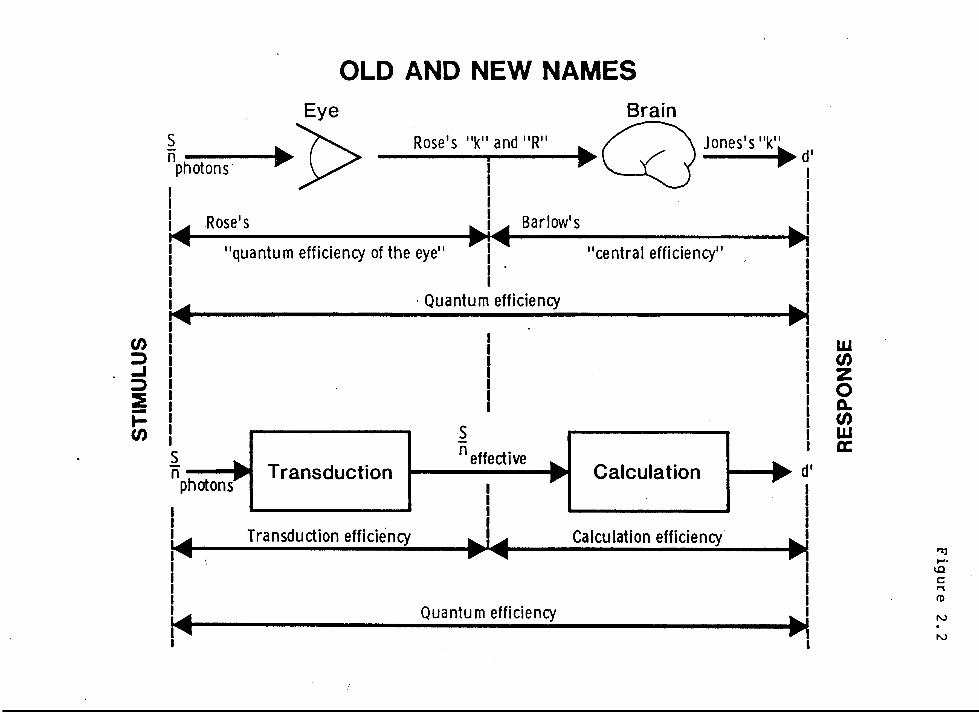
OLD AND NEW NAMES Eye Brain
~~.~ photons· y Rose's 11k11 and 11R11 C) Jones's 11k11
---...... --~_. II- d' I I
I I I .Rose• s
I I I I I I
~~ I I
.~~ Barlow's .1 .. quantum efficiency of the eye.. I 11Central efficiency.. 1
I . I I I I
~--I en I :l I ..~ I :l I ~ I i= I en' I
...... s n p hotonsJII""
I~
Transduction
Transduction efficiency
I I · Quantum efficiency IJ-:J
s n effective ....... .,.
I I I
Quantum efficiency
Calculation ....... .,.
Calculation efficiency·
I I I I _.,
w en z 0 a. en w a:
~ ...... I.Q c: ,.., (I)
I\.) . I\.)

.... en
•l
E •Ol c 0 u
Figure 2.3
lnterobser ver Variabi lit':J
a.·~o ~ 0 <t <l [E ::l
8 9
o 0 0
Standard deviation across observers
13 .,.
Noise spectral density
104 sec deg2
No noise
Signal Noise c/deg 0-!50Hz
~~ x·4• --3.3C/d,~ y :JQO
t:70ms 0-33 C/d~
300 cd/m2 lvDP1,2YAWlVA01,2,VFH1.2VLM1

'tJ 0 .r:. II) 4) '-.r:. .... .... V)
0 '-.... c 0 u
0•1
•01
I 0
Effects of noise at two luminances
0 = 3·3 cd 1m2 ,_ 130 trolands
X = 3 30 cd1 m2 "' 4000 trolands
I I I I II I
0
l 2
ncritical
I 1411111 I I ?
I II I ul -6
10
Figure 2.4
I !IIIII
2 . 2) n : Noise spectral densit\j [sec deg
Signal Noise
4 c/deg o-soHz .x:2" ·Q-&6C/dcg
y: 50 t:70ms
o- se c/deQ
I . NDP206-214

Figure 2.5
1 P------------------------------------------------
0 .. -;;; .1 lO .. ... c 0 0 ·,; 0 .r. f/) Q)
J: ._ .01
after Nagaraja (1964)
X·. 034 aJim2-. 9 trolands ~- • 34 aJ/m2-7 trolands
0· 3.4 aJ/mtso trolands
2 "critical
14. 7 disc diameter
~, __ .,A.._ __ ...._
10-5 10-4
(sec deg2
)
Noise Spectral Density

Figure 2.6
1P---------------------------------------~------~
(.)
.: .1 U)
tU ... .. c 0 0 '0 -0 .c. U) G) ... .c. 1- .01
0
after Nagaraja U964)
X • 5. 7' diameter disc /::,. ,. 14. 7' diameter disc 0 ,. 32' diameter disc
. 34 cd/m2 -7 trolands
2 n ·t· I crt 1ca
10-5 10-4
n2 [sec deg 2]
Noise Spectral Density

0 .. .. f/j tU .. .. c 0 0 , -0 J:. f/j Q)
~
Figure 2. 7
~~--------------------------------------------~
0
0
after van Meeteren and Boogaard (1973)
X • . 035 trolands /:::;., • • 35 trolands
0 · 3. 5 trolands
2 n .. cnt1cal
_ n2 [sec deg2}
Noise Spectral Density
4.5 c/deg

() .. .. U) G .. c 0 ()
"0 0 .c U) Q) .. .c ....
after van Meeteren (1973)
V •2 103 photons/( sec deg2) •. 0013 trola nds X ·2 104
II • • • 013 II
0 ·2 1o5 II ... 13 II
+ •2 106 II •1. 3 II
~ •2 107 II •13. II
2 "critical
2. 2 ddeg 7° nasal field
~,..-_ _,A.._ __ ....,,
n2
[sec deg2
]
Noise spectral density
Figure 2.8

10%
1%
TE
.1%
TRANSDUCTION EFFICIENCY
Barlow's (1977) lower bound on the fraction of corneal quanta (507 nm.) --------------that excite rods
• ',, ',
D D
'II ', II ~ ',
v...-....;,:: ' 9~ o~,',
vi .r ' ∨,\
"~ ~~~, ..,.~ ~n...' ~~. "'~· ',
to~ ~v/ ', . " '
D
011 OX
',,, X • 4 cldeg, this thesis '', O • discs, 5. 7' - 32', derived from Nagaraja (1964) ' ' ... D · 4. 5 c/deg, foveal, derived from van Meeteren and Boogaard (1973) 11 . 2 c/deg, 7° nasal field, derived from van Meeteren (1973)
.001 .01 .1 1 10 100
Trolands
X
1000
1%
.1%
10,000
"' 0

CHAPTER 3
THRESHOLDS IN.NON-WHITE NOISE 1
1 Some of the spatial-frequency tuning results were reported at the 1980 meeting of the Association for Research in Vision and Ophthalmology in Orlando, Florida (Pelli, 1980). The data on temporal tuning were collected in collaboration with A.B. Watson.

CHAPTER 3: NON-WHITE NOISE Page 87
ABSTRACT
When an observer is asked to detect a sinewave grating, is squared threshold proportional to the total noise power (including the equivalent noise) passed by a single linear filter ("channel") which depends on the signal, but not on the noise? Both hypotheses will be experimentally tested along several dimensions of spatio-temporal frequency. The hypotheses allow ·~he modulation transfer function (HTF) of the filter to be derived from thresholds measured in bandlimited noise. By bandlimiting the noise in various dimensions the MTF·may be determined over horizontal and vertical spatial frequencies and temporal frequency. In this way, the filter bandwidth (full bandwidth at half amplitude) is found to be about 7.5 c/deg horizo·ntally (for a 5 c/deg horizontal grating), .6 c/deg vertically (for 1, 3, and 9 c/deg horizontal gratings), and 16Hz temporally (for a .25 c/deg grating which was static, or temporally modulated at 4 or 16Hz).

CHAPTER 3: NON-WHITE NOISE INTRODUCTION
INTRODUCTION
Page 88
Chapter 2 found that the squared contrast threshold for many patterns is
proportional to the effective spectral density of a white noise background.
This chapter will consider how different frequency components of the noise
contribute to the threshold elevation of a sinusoidal grating. Chapter 2 was
primarily concerned with effects of noise level (of white noise). This chapter
examines effect of cut-off frequency and bandwidth (of bandlimited white
noise 2 ). The initial hypothesis will be that for any given test pattern there
is a linear filter such that the observer's squared threshold is proportional
to the total noise power passed by the filter, regardless of the noise
spectrum. Later we will acknowledge that the observer may have many such
linear filters ~vailable and need not always use the same filter to detect a
given pattern.
The assumptlons of Theory of Signal Detectability are not satisfied here,
so detective efficiency is undefined. However the finding that threshold may
be raised by noises whose spectra do not overlap the signal's spectrum is
obviously relevant to understanding why the calculation efficiency, in ·white
noise, can be so low. Furthermore, it is only by manipulation of noise
bandwidth that one can determine at what bandwidth the noise becomes white,
i.e. exceeds the bandwidth of the mechanism under study.
Several different lines of evidence suggest that human detection of
spatial-frequency gratings is mediated by independent mechanisms, "channels",
2 "Bandlimited white noise" is not white noise. White noise has a constant spectral density and frequency components with independent amplitudes over the bandwidth of the mechanism under study. "Bandlimited white noise" is white over a stated band. This band usually will not include the entire bandwidth of the mechanism under study, and thus the noise will not be white.

CHAPTER 3: NON-WHITE NOISE INTRODUCTION
Page 89
each sensitive over one or two octaves of spatial frequency (on contrast
adaptation see Blakemore and Campbell, 1969; on summation see Graham, 1977; on
masking by gratings see Legge and Foley, 1980; noise masking will be reviewed
below). We will see that effects of visual noise are consistent with this
~otion.
The approach taken here borrows much from audition. Fletcher (1940) found
that the threshold for a tone increased with increasing bandwidth of a narrow
band of noise (at constant spectral density) centered on the tone frequency, up
to a critical bandwidth beyond which further increases in bandwidth had no
effect. He reasoned that if our ear is composed of a bank of filters through
which we can detect independently then only noise which goes through the same
filter as the signal will have any effect on the detectability of the signal.
The results of a replication of his experiment by Swets, Green and Tanner
(1962) have been plotted on the right-hand side of Figure 3.1. The critical
band is 130Hz, a small fraction of the 1000Hz signal frequency. Fletcher's
notion of a critical band has been important in studies of the effects of
visual noise too, as we will now see.

0
Log c2
( re thresh in white noise]
-1
CRITICAL BANDS
VISION
( octaves re 5 c/deg ) +.I
X· 4 c/deg, from Figures 3.2 and 3.5
0 • 5 c/deg, after Stromeyer and ~ulesz (1972)
I I I I I I I I I I
7.5 c/deg
1 10
Noise bandwidth (c/deg)
0
LogE
(re thresh in white noise)
AUDITION
(octaves re 1000 Hz ) +.01 +.1 - -
0 •threshold for 1000Hz tone, after Swets, Green, and Tanner (1962)
I I I I I I I I I
130Hz
10 100
Noise bandwidth (Hz)
ttl ..... \Q c .., (I)
w . ......

CHAPTER 3: NON-WHITE NOISE REVIEW
REVIEW
Visual thresholds in non-white noise
The review will be chronological.
Page 90
Greis and Rohler {1970) used optical filtering techniques to produce a
series of photographic transparencies of low-pass-filtered one-dimensional
noise. By simultaneously projecting a sinusoidal grating and the noise they
were able to determine 2IFC contrast thresholds {60S correct) for detection of
the grating. They found that,
~As long as the spectra of signal and background overlap or at least are in close proximity, the ratio of signal and interference [i.e. noise] energies 3 is decisive for subjective detectability. When the respective spectra are separated by a certain distance on the spatial frequency axis, however, they practically no longer affect each other; the detectability of the signal improves by a considerable amount."
Pollehn and Roehrig {1970) measured threshold contrast as a function of
spatial frequency of the grating in the presence of noise backgrounds of
several different spectra. Dynamic 2-dimensional white noise raised thresholds
at all spatial frequencies, though more at middle frequencies, near 3 c/deg.
Limiting the two-dimensional dynamic noise to a narrow band {bandwidth of 1.2
c/deg and center frequency 3.3, 10, or 16.7 c/deg) raised the grating
thresholds most at the center frequency of the noise. Low-pass noise {0 to 1.2
c/deg) only slightly elevated threshold, maximally at 2 c/deg. The relative
elevation curves had a bandwidth at half height of about two octaves.
Carter and Henning {1971) found that narrow-band noise was more effective
3 By "energy" they meant contrast energy. Since the spectral density of the noise was nearly constant, constancy of their "ratio of signal and interference energies" implies proportionality of squared threshold contrast to noise bandwidth.

CHAPTER 3: NON-WHITE NOISE REVIEW
Page 91
in raising the threshold of a 160 cycle (i.e. narrow spectrum) grating while
broad band noise was more effective in raising the threshold of a single cycle
(i.e. broad spectrum) grating. This too suggests size or spatial-frequency
tuning of the detectors.
In the first thorough test of the notion of critical bands in vision,
Stromeyer and Julesz (1972) measured grating thresholds in the presence of
one-dimensional dynamic noise with- low-pass, high-pass," and band-pass spectra.
In their paper's final experiment Stromeyer and Julesz used a
constant-spectral-density band of noise centered (on a logarithmic frequency
scale) on the signal frequency. Their results have been replotted onto the
lefthand side of Figure 3.1, along with similar data of mine. Their
description is apt,
"Masking [i.e. threshold] increased as the noise band was widened, up to a critical width of approximately ±1 octave, and did not increase further when the b~nd was widened beyond this range. The results demonstrate othat a· gra·ting is masked only by noise whose spatial frequencies are similar to the grating frequency."
These results clearly distinguish our poor visual spatial-frequency
selectivity from our acute auditory temporal-frequency selectivity: the
auditory critical bandwidth is 13S of the tone frequency (or ~octave);
Stromeyer and Julesz's visual critical bandwidth (±1 octave) is about 150S of
the grating frequency.
In 1973 Harmon and Julesz reported some now-famous observations on the
visibility of block pictures of Abraham Lincoln. They started with a
photograph, isotropically low-pass filtered (i.e. blurred) to leave only
spatial frequencies up to 10 cycles per picture height. Coarse sampling (20
samples per picture height) did not reduce the information content, but yielded
a "block picture" which most people find difficult to recognize as Lincoln.

CHAPTE.R 3: NON-WHITE NOISE REVIEW
The spectrum of this block picture differs from the original only in
Page 92
frequencies above 10 cycles per picture height. By selective filtering the
authors showed that most of the masking effect was due to the sampling "noise"
in the band (10 to 40 c/picture height) adjacent to the original spectrum (0 to
10 c/picture height), while little masking was caused by sampling "noise" more
than two octaves away (i.e. above 40 c/picture height). Finally they tested
effects of isotropic two-dimensional noise bandlimited to either 10 to 40
c/picture height or 40 to 70 c/picture height. As with the sampling "noise"
the noise mask with the adjacent spectrum masked Lincoln much more effectively.
No quantitative measurements of visibility were reported.
Diagnostic radiographs suffer from quantal noise due to the limitations on
the x-ray dosage to which a patient may safely be exposed. This has led to
several studies of the detectability,of targets, usually discs, in static
noise. Chapter 2 reviewed the groundbreaking work of Sturm and Morgan (1949).
The noise in conventional radiographs has a white spatial-frequency
spectrum; its spectral density is constant up to very high spatial frequencies.
Computed-tomographic (CT) scanners have recently been introduced for use in
diagnostic radiology. It turns out that if projection data containing
uncorrelated noise are used to perform a CT reconstruction, the noise in the
reconstructed image possesses unusual correlations not found in ordinary
radiographs. Hanson (1979) determined theoretically and empirically that the
noise in the reconstructed CT image has a power spectral density proportional
to spatial frequency. Hanson produced a CT image of a target of an array of
discs arranged in columns of decreasing contrast, and rows of decreasing
diameter. He also produced a similar image with white noise instead of CT
noise. For each disc size the observer was asked to identify the last column

CHAPTER 3: NON-WHITE NOISE REVIEW
Page 93
{i.e. lowest contrast) in which he was "reasonably certain" he could see the
disc. Thresholds in white noise were approximately inversely proportional to
the disc diameter, in agreement with Rose {1948) and Sturm and Horgan {1949).
Hanson found that, relative to the white noise, CT noise produced higher
~hresholds for small discs {diameters of 3' and 6') than .for larger discs.
These results are vaguely suggestive of spatial frequency or size-tuned masking
effects, but firm conclusions are prevented by the discordance between the
frequency manipulations of the noise and the size-specific, but broad-spectrum
signals.
Chesters {1973) and Chesters and Hay {1979a, b) measured threshold
contrasts {by a modified yes-no procedure) for light and dark discs on a static
noise background. The background was a projection of photographic grain, and
thus had a white noise spectrum, except when it was defocused. They found that
defocusing the noise by 1 diopter lowered threshold only for discs with
diameters less than 15' of arc. Chesters and Hay noted that an ideal disc
detector would integrate light from the known signal area and ignore the rest
of the picture. They constructed such a detector {a photomultiplier viewing
through a signal-sized aperture) and determined the rms output as it was
scanned over the noise. They showed that defocusing the noise by 1 diopter
reduced the rms detector output only for .expected signals with diameters less
than 15' of arc, in agreement with the psychophysics. Effects for 2 diopters ]
defocus were similar, with a critical size of 30': thresholds for discs smaller
than 30' diameter fell as much as 8-fold, but there was a smaller two-fold fall
in thresholds for smaller discs, which was not predicted. Their study provides
evidence of size-specific detection.
Recently Henning, Hertz, and Hinton { 1981) used static noise backgrounds
'
CHAPTER 3: NON-WHITE NOISE REVIEW
Page 94
(randomly chosen for each observation interval) and the 2IFC method to measure
the effects of high and low-pass noise on the detection threshold of grati~gs
of 1, 3, and 6 c/deg. Using Patterson and Henning's (1977)
energy-detection-model analysis they derive filters centered on the signal
frequencies with a bandwidth of approximately two octaves at half height.
They replotted Stromeyer and Julesz's (1972) results as log threshold
versus log cut-off frequency of low- and high-pass noise and noted that the
data were symmetric: threshold in low-pass rose as the 1.3 power of cut-off
frequency, and threshold in high-pass noise fell as the -1.3 power of cut-off
frequency.

CHAPTER 3: NON-WHITE NOISE CRITICAL BANDS
CRITICAL BANDS
It may seem either obvious or mys~erious to suppose that a
Page 95
frequency-selective device is sensitive only to the total noise power passed by
a linear filter. Appendix 2 considers two possible models for a "channel": the
cross-correlation detector and the energy detector. Both models are
frequency-selective by virtue of a linear filter, and in both the squared
threshold is proportional to spectral density of white noise. However the
cross-correlation detector obeys our total-filtered-noise power hypothesis,
while the energy detector does not. Following Green and Swets (1966) and
Patterson and Henning (1977), the appendix shows that the squared threshold for
a cross-correlation detector is proportional to a weighted integral of the
noise spectrum,
(cross-correlation detector),
while for the energy detector the fourth power of threshold is proportional to
a weighted integral of the squared noise spectrum-,
(energy detector).
· If we consider only very-narrow-band white noise 5 so that 1 H( f) 1 is
approximately constant over the noise band then integration over that narrow
- The result for the cross-correlation detector is exact. The result for the energy detector neglects distortion products and is a good approximation only at high signal-to-noise ratios. Green and Swets (1966) give a good discussion of the plausibility of this assumption.
5 That is,
n2(f):n2
inside the band, and n2(f)=0 outside.

CHAPTER 3: NON-WHITE NOISE CRITICAL BANDS
Page 96
band is equivalent to multiplication by the bandwidth of the band, W,
(cross-correlation detector)
(energy detector),
or, taking the square root,
(energy detector).
Squared threshold in either detector is proportional to. the noise spectral
density, n2, and to the power gain jH(f)j 2 , i.e. squared HTF. However the two
models.depend differently on the noise bandwidth. The cross-correlation
detector's squared threshold is proportional to W, the noise bandwidth, while
the energy detector's squared threshold is proportional to tW, the square root
of the noise bandwidth.
The two models are examples, showing that proportionality of squared
threshold to noise level tells us nothing about dependence on bandwidth. The
total-filtered-noise-power hypothesis predicts that squared threshold will be
proportional to both bandwidth and spectral density of narrowband noise.

CHAPTER 3: NON-WHITE NOISE METHODS
METHODS
Page 97
Except for the differences noted below the methods of Chapter 2 apply. The main change was to bandlimit the noise to less than the bandwidth of the mechanism under study.
Signal
The signal was always a sinusoid with vertical bars, and Gaussian envelope. For some experiments the signal was also sinusoidally modulated in time.
For the first set of experiments there was no vertical attenuation. Examining the signal box of the inset in Figure 3.2 shows "x: 4°", indicating that the contrast fell to 1/e in 4° degrees horizontally, "t: 70ms", indicating that the contrast fell to 1/e in 70 ms temporally, and "y:[10°]", indicating that the grating was 10° high at constant contrast.
Noise ---In the first experiments (Figures 3.1 to 3.11, except 3.3) the noise was
dynamic one-dimensional noise. The "all-pass white noise" used in these experiments was white up to the Nyquist frequency, 23 c/deg, determined by the screen's 46 raster lines per degree. To produce low-pass or "high-pass" noise the "all-pass poise" was filtered by an appropriate 8-stage filter before the noise and signal were added and displayed.
Narrowband "heterodyne" noise with very steep skirts was produced by an amplitude-modulation technique apparently first used by Greenwood (1961). Appendix 4 presents the mathematics of this technique (and two others). An 8-stage low-pass filter with cut off at 1/4, 1/2, or 1 c/deg gave a narrow ban~ of noise centered at 0 c/deg. This then modulated a carrier of the desired center frequency. The computer synthesized both the signal and the carrier for the noise. The resulting "heterodyne" noise has very steep skirts independent of center frequency.
Heterodyne noise is white on either side of the center frequency, but not taken as a whole, because the amplitude and phases of its frequency components are s~etric about the center frequency. Appendix 3 discusses the difference in effects of heterodyne and narrowband white noise on two hypothetical detection mechanisms. Appendix 4 explains the heterodyne technique, and two methods of producing narrowband white noise which future experiments may use to avoid the theoretical problems of heterodyne noise.

CHAPTER 3: NON-WHITE NOISE RESULTS
RESULTS
The left-hand side of Figure 3.1 plots squared threshold contrast
Page 98
(relative to threshold in white noise) versus noise bandwidth (at a constant
noise level) on log-log scales. The "O"s are thresholds for 5 c/deg. replotted
from Stromeyer and Julesz's (1972) .Figure 10 (geometric mean of threshold
contrast of both observers). The "X"s are threshold for 4 c/deg replotted from
Figures 3.2 and 3.5. Each set of data has been normalized by the contrast
threshold in white noise.' The straight lines. fitted by eye. show that squared
threshold is proportional to noise bandwidth (as predicted by the total-filtered-·
noise-power hypothesis) up to 7.5 c/deg (±1 octave about 5 c/deg) and constant
beyond that. Stromeyer and Julesz noted th~ width of the critical band. but not
the log-log slope. EXamination of Figure 3.1 shows that their data do not
cover a sufficiently wide range of bandwidths to distinguish between slopes of
1/2 and 1 for squared threshold versus noise bandwidth. This result is
consistent with cross-correlation detection and inconsistent with energy
detection. The analogous auditory experiment is plotted on the right hand side
of Figure 3. 1
Figure 3.2 shows threshold for a 4 c/deg signal as a function of the
spectral density of narrowband noise centered on 4 c/deg. The "X"s show
results for a noise bandwidth of 2 c/deg. The triangles show results for ·a
noise bandwidth of 1 c/deg. The smooth curves (fitted by eye) show that
squared threshold is proportional to the sum of the critical and actual
spectral densities. The critical spectral densities are 5.3 x 10⁻⁷ sec deg and
1.26 x 10⁻⁷ sec deg for noise bandwi~ths of 1/2 and 2 c/deg. respectively.
This is unlike masking by gratings: there is only the barest hint of
facilitation (near the knee of the curve the average threshold is about one

0
Log c2
[ re thresh in white noise)
-I
CRITICAL BANDS
VISION
[ octaves re 5 c/deg ) +.I
X • 4 c/deg, from Figures 3. 2 and 3. 5
0 · 5 c/deg, after Stromeyer and Julesz (1972)
I I I I I I I I I I
7. 5 c/deg
I IO
Noise bandwidth [c/deg)
0
LogE
[re thresh in white noise)
AUDITION
[octaves re IOOO Hz ) + .OI +.I - -
0 -threshold for IOOO Hz tone, after Swets, Green, and Tanner (1962)
I I I I I I I I I
I30 Hz
IO IOO
Noise bandwidth (Hz)
I'll ..... \Q c ""' fT)
w • ....,

'0 0 s: ., ~ .. .. ., f g u
The effect of narrowband noise center.d on the signal frequency
•1
•OJ
t01
X• noise
A• noise
I • L I ...,, I I lleel
0 No noise
bandwidth Of 2 c/deg bandwidth ot 112. C/deg
I 1 I I tel I I I I I el I I I I I el ''"""
Noi$e spectral density [sec deg 1
w

CHAPTER 3: NON-WHITE NOISE RESULTS
Page 99
standard error, 1 dB, below the zero-noise threshold), and the log-log slope is
1, not .6. At high spectral densities squar~ threshold is proportional to
noise level. This suggests repeating the following experiments at twice the
noise level would only double the squared thresholds.
We have already seen that squared threshold in wideband noise is
proportional to spectral density. · Figure 3.2 plots threshold of a ~ c/deg
signal as a function of the noise level of a narrow band of noise centered on
1 There were several small differences between the experiments.
Stromeyer and Julesz used a n~ise le!gl of n2:6.9 10-6 sec deg, while my points are from a noise level of n =21 10 sec deg. It is unlikely that this difference in noise level matters, given the proportionality of squared threshold to noise level of both narrowband noise (see Figure 3.1) and broadband noise (see Chapter 2).
Stromeyer and Julesz's noise bands were symmetric about the signal frequency on a logarithmic scale (e.g. ±1 octave about 5 c/deg = 2.5 to 10 c/deg). My narrowband noise was symmetric on a linear frequency scale (i.e. 3.75 to ~.25 c/deg, and 3 to 5 c/deg, taken from Figure 3.2), and my broadband noise went down to zero frequency (i.e. 0 to 10 and 0 to 20 c/deg, taken from Figure 3.5).
In principle their method ("The subject adjusted the grating to threshold with a 1-dB step attenuator") is susceptible to criterion variations on the part of the observer. This seems particularly undesirable since a noise background that is always visible makes the observer's task more subtle than just determining whether or not the screen appears blank. There is evidence of this problem in their Figure 10 which shows the effect of noise bandwidth. As the noise bandwidth is increased most of the threshold curves oscillate up and down by more than ~ standard errors. It seems reasonable to expect that threshold should rise monotonically as the bandwidth of a noise mask is increased. They suggest that "the subject may adopt a different threshold criterion for judging gratings in narrowband vs. broad-band noise." My experiments avoided this problem by using 2AFC. Thresholds determined as a contrast required for a certain proportion correct responses on 2AFC are, at least in principle, immune to criterion variations (Green and Swets 1966). However the replot of Stromeyer and Julesz's data in Figure 3.1 (geometric mean of threshold contrasts from both their observers) shows that their results are very similar to mine in form though with somewhat more variability. It would seem that method- of adjustment can provide similar results to those found with a criterion-free method, but that the standard errors are misleading because they can be smaller than the variations due to systematic variations of criterion from condition to condition and from observer to observer.
CHAPTER 3: NON-WHITE NOISE RESULTS
Page 100
the signal frequency. TWo bandwidths were used, 1/2 and 2 c/deg. The curves
(fit by eye) show that squared threshold is proportional to actual plus critical spec· ~l
density for these narrowband noises too. Quadrupling the bandwidth of the
noise, from 1/2 to 2 c/deg, approximately quadrupled (the ratio is 4.2:1) the
squared threshold for detect~on, as predicted by the total-filtered-noise-power
hypothesis.
As noted in the Methods section, these experiments did not use narrowband
Gaussian white noise (whose components are stochastically independent), instead
they used heterodyne noise (which has a symmetric spectrum: the amplitudes and
phases are s~etric about the center frequency of the band of noise).
Appendix 3 evaluates the consequences of this on cross-correlation and energy
detectors, and Appendix 4 shows how future experiments might create narrowband
Gaussian white noise, and thus avoid the theoretical problems of heterodyne
noise.
There is one point in common between the heterodyne and ,
narrowband-white-noise masking data. When the noise band extended from 0 to 2
c/deg, Figure 3.2 (which used heterodyne noise) reports a threshold 9 dB higher
than Figure 3.4 (which used narrowband white noise). Since the noise contrasts
used differed by almost the same amount (ratio of 9.5 dB) the agreement is
excellent. Thus, at least at this point, heterodyne noise had the same effects
as narrowband white noise.
In the following sections various experiments will be presented that
manipulate the noise spectrum in various dimensions. The particular choices of
the type of noise were pragmatic; spectral manipulation of video signals is
difficult. However each experiment varied the noise bandwidth in only one
dimension, while the othe.r spectral dimensions were kept fixed, and the
J I

CHAPTER 3: NON-WHITE NOISE RESULTS
Page 101
total-filtered-noise-power hypothesis may be tested again and again in these
different contexts.

CHAPTER 3: NON-WHITE NOISE CRITICAL BAND: ORTHOGONALLY
CRITICAL BAND; ORTHOGONALLY
Page 102
One of the important differences between vision and audition is the
greater number of dimensions of visual stimuli. It is reasonable to ask what
the channel's tuning is in the dimension orthogonal to the grating. The last
section used one-dimensional dynamic noise, i.e. the vertical bandwidth was
very small. This section will use two-dimensional dynamic noise. Various
vertical bandwidths were used, but the horizontal bandwidth (33 c/deg) was
sufficient to be called white. This was confirmed by finding identical results
after increasing the bandwidth to 99 c/deg.
The two-dimensional spatial frequency of a horizontal 4 c/deg grating
(i.e. with vertical bars) is
We have seen that squared threshold was proportional to noise bandwidth in the
horizontal dimension about the 4 c/deg test frequency. Here we ask if squared
threshold is proportional to noise bandwidth vertically, about the 0 c/deg
frequency of the test in that dimension.
Method
Three signal frequencies were used, 1, 3, and 9 c/deg, wtth circularly symmetric envelopes, falling to 1/e on a radius of 1.3° from the peak.
In this experiment the bandwidth o( two-dimensional dynamic white noise mask was systematically reduced in the (vertical) dimension orthogonal to the (horizontal) frequency of the test gratings. The vertical bandwidth was controlled by adjusting the clock rate of the noise generator. The Nyquist frequency (half the sample rate) was taken as the nominal bandwidth of the noise. The horizontal bandwidth was independent of these clock rate manipulations.
The data in Figure 3.3 were collected at two viewing distances in order to ascertain whether the maximum attainable noise bandwidth (33 c/deg) at the normal viewing distance was effectively infinite. Tripling the bandwidth to 99

CHAPTER 3: NON-WHITE NOISE CRITICAL BAND: ORTHOGONALLY
Page 103
c/deg (by increasing the viewing distance 7 ) did not significantly change thresholds so the results at both viewing distances have been combined.
Results
Figure 3.3 plots contrast threshold versus vertical bandwidth. As the fitted
lines show, squared threshold is proportional to noise bandwidth, up to a
critical bandwidth of about .6 c/deg, and constant beyond that. The fit to the
1 and 9 c/deg results is good; the fit to the 3 c/deg results is only fair.
The critical bandwidths are .remarkably narrow, and imply linear
integration, vertica~ly, over at least a degree. This suggests the channels
were well matched to the 2.3° vertical extent (at half-height) of the grating.
A cross-correlation by the (known) signal would. have a critical bandwidth of
.27 c/deg, 8 which .is about half that of the human observer.
It is surprising that the critical bandwidth should be the same for test
frequencies differing by nearly an order of magnitude, but this result may
depend on using, as here, the same vertical extent for all spatial frequencies.
7 In case the reader misunderstand, I hasten to add that changing the viewing distance involved more than just taking a few steps backward. It required increasing the power of the noise in order to keep the same spectral density, increasing the physical scale of the signals in order to keep the same spatial frequency and extent (from the observer's point of view), and reducing the cut-off frequency of the low-pass filter in order to keep the same vertical bandwidth (from the observer's point of view). ·
• A vertical weighting fUnction of e-(y/1.3°)2
has a Fourier transform,
1.3o lw e-(fy 1.3o lw)2•
The critical bandwidth (single-sided) is
1~ [e-<fy 1.3° lw)2
]2 dfy
= 1 /( 1. 3° 2 12)
= • 27 c/deg.
Figure 3. 3
Effect of the orthogonal bandwidth of the noise.
·1
6
cox a-~ ~
-r~ x
0 ~-co-.s:::; en «>
~~ '-s::. +'
+' x 1 c/deg en
/ 0
3 c/deg '- 0 +' c 0
~ 6 9 c/deg
u •01
x j critical · ~ j bandwidth
I IL~------~'-L'~'~'~'•'~"~--L--4~~·~·~•u!l~l--~,._~~·~·~·~·~.! ---, r 0 ~ 1
• Cutoff frequency [c/deg]
f •
10
.
.
Signal Noise 0-50Hz
• .:x::1·3· • y: 1•3" O-j c/deg
t:70ms 0-33 c/deg(neor) 0-99 c/deQ(for)
3oocd/m21 NDP236 -248
2 -6 n = 10 sec deg2

CHAPTER 3: NON-WHITE NOISE CRITICAL BAND: ORTHOGONALLY
Page 104
Assuming that the each channel's tuning is separable into horizontal and
vertical spatial frequencies, the .6 c/deg critical bandwidth vertically
implies orientation tunings of ±17° at 1 c/deg, ±6° at 3 c/deg, andt2° at 9
c/deg. Campbell and Kulikowski (1966) determined the orientation tuning for
~asking by narrowband one-dimensional dynamic noise. Threshold for a 10 c/deg
vertical grating as a function of mask orientation had a bandwidth of ±12° at
half height. Their ±12° tuning (at 10 c/deg) is much broader than the ±2°
tuning (at 9 c/deg) deduced here on the assumption of separability. Clearly
the two-dimensional spatial frequency tuning for detection of a grating needs
more research.

CHAPTER 3: NON-WHITE NOISE SPATIAL-FREQUENCY TUNING
SPATIAL-FREQUENCY TUNING
Page 105
The review of the vision literature on thresholds in non-white noise
showed that detection seems to be mediated by frequency-selective mechanisms,
"channels". However no one has yet collected data on thresholds in noise which
would distinguish various models of a frequency-select! ve channel. We have
seen that squared threshold is proportional to the critical plus actual
spectral densities of white noise (Chapter 2), and narrowband noise (Figure
3.2).
The hypothesis that squared threshold is proportional to total noise power
at the filter output implies that the squared threshold in the presence of a
sum of two noises with non-overlapping spectra should equal the sum of the
squared thresholds in the presence of each noise alone.
This will be examined in several ways. Figure 3.2 will compare thresholds
in 1 and 2 c/deg bandwidth narrowband noise, but the crucial test will come
from measurements of threshold in low-pass, high-pass, and narrowband noise.
All the experiments will use high noise levels so that threshold is raised
many-fold over its noise-free value, and thus the equivalent noise may be
neglected.
The experimental test rests on the fact that low-pass noise or high-pass
white noise may be described as a sum of narrowband noises occupying
contiguous, non-overlapping bands. The question is whether the squared
thresholds in low- or high-pass noise may be predicted by the sum of the
squared thresholds in the component narrowband noises. Or, conversely, is the
squared threshold in narrowband noise from f-~ to f predicted by the difference
of the squared thresholds in low-pass (or high-pass) noise with·cut-off

CHAPTER 3: NON-WHITE NOISE SPATIAL-FREQUENCY TUNING
frequencies of f-6 and f c/deg?
Page 106
If the hypothesis succeeds then we may conclude that squared threshold is
proportional to the noise power passed by a linear filter whose squared
modulation transfer function is given by the plot of squared threshold versus
center frequency of narrowband noise.
Published data on thresholds in noise are not suitable for a thorough test
of the linear filter hypothesis. Stromeyer and Julesz (1972) and Henning,
Hertz, and Hinton (1981) reported threshold in high- ~nd low-pass noise. For
our test we would need measurements with high- and low-pass noise at each
cut-off frequency, but they used only low-pass noises with cut-off frequencies
below the signal frequency, and only high-pass noises with cut-off above the
signal frequency. They do report high- and low-pass thres~olds with cut-off at
the signal frequency, and according to our hypothesis the sum of the squared
thresholds in high and low-pass noise with the same cut-off frequency should
equal the squared threshold in all-pass noise. Unfortunately Stromeyer and
Julesz did not report the three measurements in a compatible way. For all-pass
·noise the absolute threshold is reported, while for the low and high-pass
noise, thresholds were reported only as elevations relative to threshold in the
absence of noise, which was not reported. The Henning et al. result will be
discussed along with mine.
Methods
The methods were exactly as described for Figure 3.2.
Results
Figure 3.4 plots (as "0") threshold of a 4 c/deg grating as a function of
the center frequency of a band of noise 1 c/deg wide. Interpreted as a channel

'"0 0 ~ Ul Cl1 L.. ~ ~
~
Ul c L.. ~
c 0 u
Figure 3. 4
The effect of narrowband noise
1
·3
·1
·03
·01
·003
x =noise bandwidth of 2 cldeg
o = noise bandwidth of 1 c I deg
X
tsignal
·~·~·~·~·~·~'----_.--~·--~·~·~·~·~·~•ul _________ l~l~ 3 10 30' CXJ 1 No
Center frequency of the noise (c/deg) noise
r---------~----------Signal Noise
4c/deg 0-~Hz (300ms]
-AA~hA~~;~ • ~vv~~vv- t:70ms x•l- 1 tof•1c/deg
O•f-~ tofe-!5<:/deg
3:50cd/m2 I NOP447-74

CHAPTER 3: NON-WHITE NOISE SPATIAL-FREQUENCY TUNING
Page 107
shape, the fUnction has a full width at half maxtmum of one octave {i.e. 3
c/deg to 6 c/deg). Results for a 2 c/deg noise bandwidth are also plotted (as
"X"). The solid curve through these results is a prediction from the narrower
bandwidth results. Squared threshold in each 2 c/deg band of noise is predicted by the sum of squared thresholds in the 1 c/deg component bands of noise.
Figure 3.5 plots threshold as a function of cut-off frequency of high-pass
{"X") or low-pass {"0") noise. The continuous curves are predictions from the
narrowband noise data {for details see below: "off-frequency seeing"). The set
of measurements was made three times, but only the last set is shown. Each
repetition found lower thresholds for those conditions in which the cut-off
frequency of the noise was near the signal frequency. The final repetition
gave the results shown. The fall in threshold from the second to the third set
of measurements was small, suggesting that an asymptote had been reached.
Figure 3.9 documents this practice effect, which will be discussed fUrther
below ("Off-frequency looking").
The next experiments compare results with several test frequencies.
Figure 3.6 plots the threshold of 4 c/deg {replotted from Figure 3.4) and 2.5·
c/deg (plotted as "0") signals as a function of the center frequency of 1 c/deg
bandwidth narrowband noise. A curve connecting all the 4 c/deg results, after
shifting to the left by 2.5:4, provides a passable fit to the 2.5 c/deg
results.
In Figure 3.7, thresholds in low-pass noise are plotted for signal
frequencies of 2.5 ("A"}, 3 ("X"), and 4 c/deg {"0", replotted from Figure
3.5). The curves have very similar shapes, differing principally in having
slightly different asymptotes in all-pass noise. If the three signal
frequencies had been detected by the same channel then the curves would have
been vertical translations of one another, reflecting the channel's different
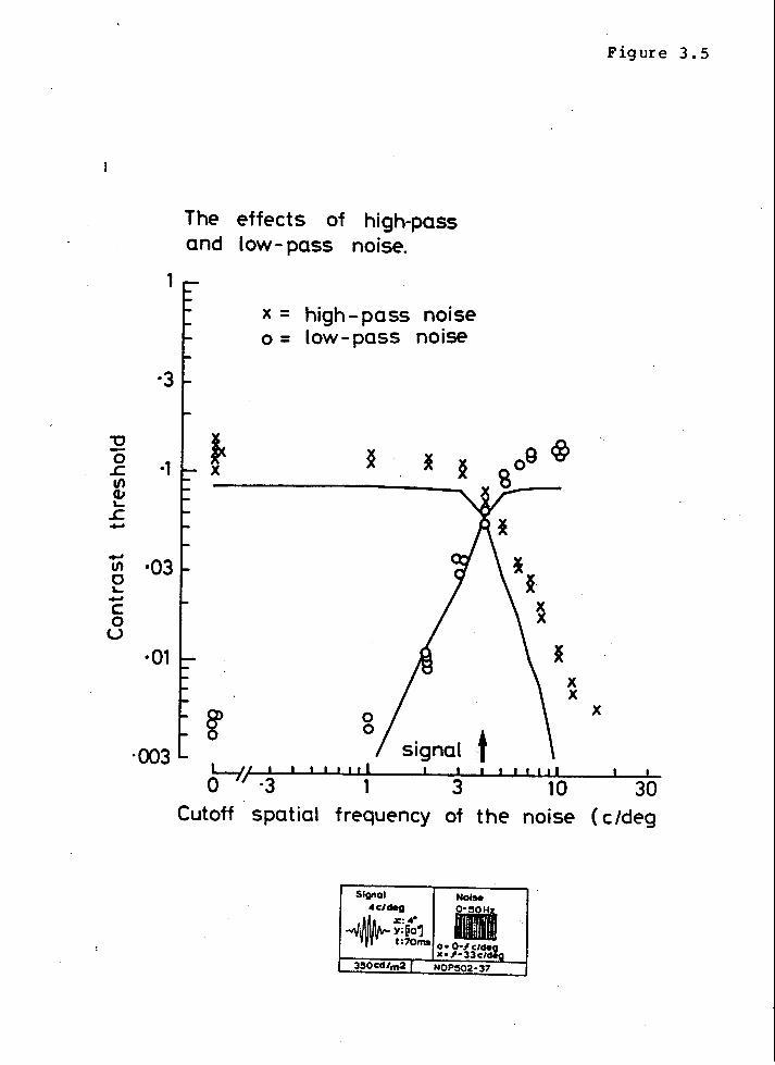
1
·3
"0 0 .c ·1 fl) ell '-.c .....
..... ·03 fl)
c '-..... c 0 u
·01
·003
The effects of high-pass and low- pass noise.
x = high-pass noise o = low-pass noise
~ ~ l ~ X
§> 0 0
signal H' I I I I I I I l I 0 r ·3 1 3
~
X X
* X X
t I I I I II
10 Cutoff spatial frequency of the noise
Signal Noise 4C:Ideg .1 ~%·4· ·.
~ y;~o"j t:70ms
O• O·.lctdeg x•.l-33ctdeg
3~0C:d/m2 I NOP~2-37
Figure 3. 5
X
I
30 ( c/deg

-c -0 .c. en ClJ L.. .c. .., .., en c L.. ..... c 0 u
1
·3
·1
·03
·01
·003
Figure 3. 6
The effect of narrowband noise on two different signal frequencies.
o=2·5 c/deg signal 4 c/deg signal
(
I I Ill .I tl t ~i~7~:1 ·3 1 3 10 30
Center frequency of the noise ( c /deg)
:f Signal Noise 2•5C/deg 0-50Hz +X:4" • y:Oo"j
t:70ms lf_-·5 to_i_•·5c/d_~
35QCd/m21 NDP466-79

.... en 0
1
·3
!: ·03 c 0 u
·01
Figure 3. 7
The effect of low-pass noise - on thr~ signal frequencies.
~ = 2·5 c/deg signal x = 3 c/deg signal o = 4 c /deg signal
·003 L_/1 I I I I I I I I ~,
tt! signals I 111111
0 ·3 1 3 10
Cutoff spatial frequency of the noise (c /deg)
Signal Noise 0-50Hz
350Cd/m2

CHAPTER 3: NON-WHITE NOISE Page 108 SPATIAL-FREQUENCY TUNING
sensitivities to the three signal frequencies. Instead the curves translated
with the signals along the frequency axis suggesting that near 3 c/deg there
must be at least one channel every .5 c/deg. Thus near 3 c/deg the channel
density is at least 4 channels per octave.
According to the total-filtered-noise-power hypothesis threshold in low-
or high-pass noise should be sums of threshold in narrowband noise. The
continuous lines in Figure 3.5 are predictions of the low-pass and high-pass
results from the narrowband results of Figures 3.4. The predictions are much
too low, particularly for all-pass noise.
A similarly unsuccessful prediction may be made using just the low- and
high-pass data. Low- and high-pass noise with the same cut-off frequency are
complementary parts of all-pass noise. Figure 3.8 shows predictions of the
squared all-pass threshold by the sum of complementary squared low- and
high-pass thresholds as a function of the cut-off frequency. The prediction is
too low by about 2 dB near the signal frequency.
The next section will interpret these discrepancies as evidence that the
observer used different channels when the noise was primarily above or below
the 4 c/deg test frequency.
In this section we have tested two aspects of the
total-filtered-noise-power hypothesis. In order to highlight the importance of
these tests, two simple detectors were considered as examples. The hypothesis
predicts that squared threshold should be proportional to noise level (true of
both cross-correlation and energy detection), which was confirmed, and
bandwidth of narrowband noise (true of cross-correlator, but not of energy
detector) which was also confirmed. Furthermore the hypothesis predicts a very

Q) (/)
0 c: (/) (/)
0 a. I --0
c: ·-
+(/)
0 '-+-c: 0 u
.3
.2
. 03 0
Summing the effects of high· and low pass noise
to predict the effects of all pass- noise
signal
2 4 6 8 10 12
Cut off frequency of the low and high pass noises ( c/deg)
1"1] ..... lQ
C>C c ,., I'D
w . (X)

CHAPTER 3: NON-WHITE NOISE SPATIAL-FREQUENCY TUNING
Page 109
general additivity: the sum of squared thresholds in several independent noises
should equal the squared threshold in the sum of the noises•.
Attempts to predict the effects of low and high-pass noise from those of
narrow-band noise met with failure. Similarly, thresholds in low and high-pass
noise with the same cut-off frequency underestimated the all-pass threshold
when the cut-off frequency was near the signal frequency. The assumption that
a signal is always detected by the same channel will now be dropped.
Off-frequency looking
Fletcher's critical band technique is not well suited for determining the
MTF of the channel filter since the channel filter may be asymmetric.
Patterson (1974) measured auditory thresholds for a tone as a function of its
distance in frequency from the edge of a broad band of noise with very sharp
skirts. Patterson's analysis assumed that a given signal is always detected by
the channel with maximum gain at the signal frequency. It was subsequently
realized that in the presence of noise at only one side of the signal frequency
the best signal-to-noise ratio would in general be obtained by a filter whose
maximum sensitivity was near but not at the signal frequency. Patterson and
Nimmo-Smith ( 1980) found that their observers could listen "off-frequency" to
lower their thresholds by as much as 5 dB.
An analogous off-frequency looking hypothesis is given partial support by
the evidence that off-frequency looking seems to require practice. One might
' This assumes each noise has sufficient power to raise threshold well above the zero-noise level. More generally, the prediction is that the sum of squared thresholds (each minus squared zero-noise threshold) in several independent noises should equal the squared threshold (minus squared zero-noise threshold) in the sum of the noises.
CHAPTER 3: NON-WHITE NOISE SPATIAL-FREQUENCY TUNING
Page 110
expect that when first presented with a detection task an observer would use a
channel centered at the,signal frequency, and would only gradually learn to
look off-frequency as he notices correlation b~tween appearance and the
subsequent feedback. Figure 3.8 shows prediction of the (squared) all-pass
threshold by the sum of squared low- and high-pass thresholds. There is a
discrepancy when the cut-off is near the signal frequency. Henning, Hertz, and
Hinton (198t) found this too.
A complete set of thresholds in low- and high-pass noise were measured
·three times. Figure 3.9 shows the effect of practice for three conditions of
interest: all-pass noise, and low- and high-pass noise with cut off at the
signal frequency (4 c/deg).
As reported in Chapter 2, threshold in all-pass noise showed no systematic
change with practice. Grouped by days, the second day thresholds in all-pass
noise were slightly higher that each of·the other days (T-test significant at
the • 1 level), but all-pass thresholds were essentially the same on the first,
third, and fourth days (T-test not significant at the .1 level).
Improvement with practice is evident in both low- and high-pass noise
conditions. Grouped by days the thresholds fn high-pass noise fell about 40~
(5 dB) and the threshold in low-pass noise fell about 30S (3 dB) from the first
to the last day. A T-test showed that both differences are significant at the
.025 level.
The channel shape derived by Patterson and Nimmo-Smith was in good
agreement with that found by Patterson (1976) using notch noise (i.e. white
noise with a narrow frequency band removed), a technique designed to minimize
off-frequency listening, but was twice as broad as that derived by earlier
(

The effect of prac1ice on thresholds in noise
+
.I
--+------------- + . + + + .,.,. ...... ----.__.....,__ ____ ------ __ ....._- -+- -t +
t ___ -t:_ ___ + :,:T1:-F------±-in all-pass noise (Q-30 c/deg)
+
0
0 in high-pass noise (4-30 c/deg)
.I
X
.)( -----)0(,------x-- X
in low-pass noise (0-4 c/deg) X)( x X
--- --~-· w . "" March 18 March 23 March 25 March 27

CHAPTER 3: NON-WHITE NOISE SPATIAL-FREQUENCY TUNING
Page 111
studies using narrow-band, or low- or high-pass noise (e.g. Patterson 1974).
The notch-noise technique is elegant, but requires assuming that the channel is
symmetric on a linear frequency scale, which is nearly true in audition, but is
manifestly false for spatial-frequency channels in vision.
Assume that threshold is always determined by the filter with the best
signal-to-noise ratio, s/n • What filter shape would give rise to the data of
Figures 3.4 and 3.5? Patterson and Nimmo-Smith (1980) attempted to answer a
similar question for their hearing data but found that the filter shape
"solution" was unstable, that is, insignificant changes in the data produced
violent changes in the solution. They overcame the difficulty by constraining
the solution. They assumed the channel shape could be described by·a "rounded
ex.ponential", ( a+bx+cx2+dx3 )e-k I xI • This function has the parameters a b c d ' ' ' '
and k, to adjust the shape in various ways, but constrains the solution to
conform to their prior belief that the channel has a roughly Gaussian shape.
One would like the experiment to dictate the model. Allowing the data
only to adjust a few parameters of an assumed model fails to satisfy this
desire. However by the total-filtered-noise-power hypothesis squared threshold
is a weighted integral of the filter's squared MTF over the noise band. Small
wiggles in the filter shape would not affect the results of Figure 3.5. Indeed
Patterson and Nimmo-Smith's solution contained non-monotonic wiggles on both
skirts of the filter which they dismissed as artifacts of the "rounded
exponential". The wiggles may indicate that their constraints were only just
sufficient to obtain a stable solution.
I have less data than they did. Therefore I must constrain the solution
more narrowly. We will assume the MTF has the form,

CHAPTER 3: NON-WHITE NOISE Page 112 SPATIAL-FREQUENCY TUNING
IH{f)l = 1
Appendix 5 shows that if the channels all have this "flat-top power law" shape
then {1) one channel should account for all the low-pass noise thresholds and
the threshold in narrowband noise below the signal frequency, and {2) a second
channel should account for all the high-pass noise thresholds and the
thresholds in narrowband noise above the signal frequency.
Figure 3.10 shows fits of this flat-top power law model to the low- and
high-pass data {assuming the total-filtered-noise-power hypothesis applies to
each channel). Initial fits yielded similar slopes for the skirts so the
channel was constrained to be symmetric {i.e. l=h in the.above equation). The
center frequency was varied independently for the low and high-pass data. The
best fitting bandwidth was 1.5 octaves {at half height) for the low-pass data,
and 2 octaves for the high-pass data; both fits are shown.
The fits were made by eye. This was straightforward because the sloping
parts of the data determine the steepness of the skirts, so for each bandwidth
that I selected, a simple computer program determined the center frequency
which would correctly predict the all-pass threshold.
Figure 3.11 shows prediction of the narrowband thresholds from the best
fit to the low- and high-pass thresholds. As discussed above the expectation
is that one channel describes the high-pass and
narrow-band-above-signal-frequency results, and that another channel describes
the low-pass and narrow-band-below-signal-frequency results. This expectation
is largely born out; the largest discrepancy is that the

1
·3
-o -0 ·1 .J: en Cll ~
.J: ....,
...., ·03 en
c ~ ...., c 0 u
·01
·003
The effects of high-pass and low- pass noise.
x = high-pass r)Oise o = low-pass noise
~------- T --~ .. , X ~'
g> 0
0 0
signal t
Figure 3.10
{f-11 ·J I I I I I I { 3 I I I I 1b 30 Cutoff spatial frequency of the noise ( c Jdeg
Signal Noise 4C/deg I. ~x·-4• --4 y;~o1
t:10ma O• 0-~c/deg x•.l•33cldig
3!50cdlm21 NOP!502·37
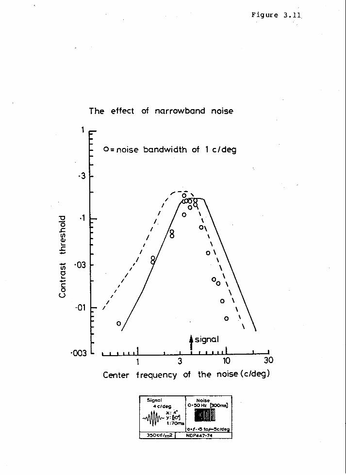
1
·3
"'0 ·1 0 .J.: Ul ell ~
.J.: -·03 -Ul
0 ~ -c 0 u
·01
·003
Figure 3.11.
The effect of narrowband noise
o =noise bandwidth of 1 c I deg
\
I ' I o\ I \ .,
I \ I \
I 00 ' I
I \ I
I 0 ' I
' 0 \ 0 \
I I I I I tsignal
I I I I I I I .I 1 3 10 30
Center frequency of the noise ( c/deg)
Signal 4c/deg
-AA~~ftll~ ~; ~ ~vy~~vv- t :7oms
o•l--'!5 to,._5ctdeg 350cd/m2 NOP447-74

CHAPTER 3: NON-WHITE NOISE SPATIAL-FREQUENCY TUNING
Page 113
narrow-band-above-signal-frequency thresholds are almo~t a factor of 2 lower
than the prediction. The appearance of the graph suggest that the observer may
have used a channel with an even lower center frequency.

i.
CHAPTER 3: NON-WHITE NOISE TEMPORAL TUNING
TEMPORAL TUNING
So far we have examined spatial-frequenQy tuning in both spatial
Page 114
dimensions. This section investigates temporal frequency tuning. The data
were collected in collaboration with A.B. Watson in 1979.
Method
The most analogous. technique to that of the previous sections would be to use one- or two-dimensional dynamic white noise, bandltmited to a range of temporal frequencies. However, this was not technically possible with the equipnent available to us. Therefore we adopted a simpler technique within our technical capabilities. The signal parameters and observer CAB) were the same as in Watson and Robson (1981, they called AB, "ABWU) to allow comparison with the temporal tuning they derive from frequency discrimination.
The signal was a 1/4 c/deg grating, and the noise was a randomly flickering 1/4 c/deg grating. The creation of both signal and noise began with a "master" 1/4 c/deg grating with a Gaussian envelope over space ·.(6° radius to 1/e) and time (250 ms to 1/e).
master(x,y,t) = sin(2~x)
The signal was an attenuated version of this master, temporally modulated at either 0, 4, or 16 Hz,
signal(x,y,t) = c cos(2wftt) master(x,y,t)
The noise was the product of the master and a random temporal modulation, r(t),
noise(x,y,t) = r(t) master(x,y,t).
The modulation, r(t), was bandlimited white noise. In the terminology of Appendix 1, the noise was dynamic and zero-dimensional because it varied . randomly only over time. The "all-pass" white noise referred to in the text extended from 0 to 40 Hz. Low-pass and high-pass noise were derived by ' filtering the "all-pass" temporal noise prior to modulation of the 1/4 c/deg master.
The generation of the stimuli may be described in several steps. The computer synthesized the master pattern via a digital-to-analog converter. To produce the signal the master pattern was multiplied by the appropriate temporal factors (via a multiplying digital-to-analog converter) and attenuated. The (programmable) attenuator controlled the contrast, c, and produced the temporal Gaussian envelope.
-Production of the noise involved more steps. The computer synthesized
·temporally whi t.e .noise (one sample per frame) which was low-pass filtered by an 8-stage filter with cut-off at 40 Hz (which was below the 50 Hz Nyquist

CHAPTER 3: NON-WHITE NOISE TEMPORAL TUNING
Page 115
frequency). This was then either low- or high-pass filtered by another 8-stage filter. This bandlimited noise was sampled (via an analog-to-digital converter) once per frame. To produce the displayed noise, the master pattern was multiplied by the current noise sample (via a multiplying digital-to-analog converter) and attenuated. The (programmable) attenuator controlled the noise level and produced the temporal Gaussian envelope.
Finally the signal and noise were added and sent to the display.
The entire apparatus was carefully calibrated and checked for artifacts. Five alternate arrangements had previously been rejected because of artifacts which we ultimately traced to substantial feedthrough from the digital input of the multiplying digital-to-analog converters (MDACs) to their output, even when 0 volts was presented to their analog input. This characteristic is not usually specified by manufacturers of MDACs, so we eliminated the problem by changing the digital input to the MDAC only between frames.
Results
Figure 3.12 illustrates the temporal characteristics of ·the signals.· Each
temporal envelope is shown above its Fourier transform. The Gaussian envelope
(with 250 ms time constant) of the stimuli determines their bandwidth at about
2Hz full width at half height, except for the 0 Hz signal whose bandwidth is
half that.
Figure 3.13 plots threshold versus noise spectral density of white (0-40
Hz) noise. The curve shows that squared threshold is proportional to the
critical plus actual spectral density of the noise.
Figure 3.14 shows thresholds for 0 and 4Hz signals in high-pass noise.
Figure 3.15 shows thresholds for 4 and 16Hz signals in low-pass noise. In
each case the two signals yield distinct curves, not vertically displaced
copies of each other, indicating that the signals are detected by different
channels.
According to the total-filtered-noise-power hypothesis, the squared
threshold due to narrowband noise, e.g. from 2 to 4 Hz, is the difference in
squared thre~holds in high-pass (or low-pass) noise due to changing the cut-off

Figure 3.12
The temporal envelopes and their amplitude spectra.
...... ·3 Q_
E 0
OJ >
...... 0 OJ
·01
0:: ·003
OHz 4Hz 16Hz
L -- ··- ·-
j s;gnal ~I 0 1
Temporal frequency ( Hz)

\J 0 .c lll <1.1 '-.c
·1 +-'
+-' lll d '-+-'
c 0 u
·01
The effect of temporal noise
Signal ·25c/deg 16Hz
•
. :x::s• y: s· t:250ms
Noise
·25c/deg
•
:x::s• y: s• X t:250ms
0-40Hz
I I l I 111
n2
: Noise spectral density [sec]
Figure 3.13
X
!I IIIII

1j
0 .1: ·1 t/) (1J '-
.1: .....
..... t/)
0 ·3 I.... ..... c 0 u
Figure 3.14
The effect of temporally high- passed noise.
o = 0 Hz signal • = 4Hz signal
TAB46-58
Cutoff frequency of the noise ( Hz )
f
0 0

Figure 3.15
The effect of temporally low-passed noise.
1 Signal Noise ·25c/deg ·25 c/deg
• =4Hz signal
~~ x·a· ·x·a· • ""'\~ \IV'- Y =· a• y:· a• X . 1 t:250ms t:250ms
0-5 Hz
340CdJm2 TAB36- 45, 59-a2
·3 o =16Hz signal 0
"C 0
.J: ·1 Vl
CIJ ~
.J: .....
..... Vl 0 ·03 ~ ..... c 0 u
·01
·003
Cutoff frequency of the noise (Hz)
f

... Ill 0 L..
·1
c ·03 0 u
"0 <lJ
u ·01 "0 <lJ L..
a..
·003
Figure 3.16
Estimated channel sensitivities (predicted effect of narrow band noise).
Derived from :
0 = 0 Hz signal, high pass noise data
e =4Hz signal, high pass noise data
• = 4Hz signal,low pass noise data
0 = 16Hz signal,low pass noise data
tsig~~~~~---L--~~~~t_s~~g~~~?~:~.I~_·I~s~!_g_n~?~', 0 3 10 30
(noise) frequency (Hz)

CHAPTER 3: NON-WHITE NOISE Page 116 TEMPORAL TUNING
frequency by the appropriate amount (in our example, from 2 to 4Hz). Given
the total-filtered-noise-power hypothesis, narrowband noise thresholds are
proportional to the channel's MTF.
Figure 3.16 shows these predicted thresholds in narrowband noise, except
that, since the cut-off frequencies were not evenly spaced, the plotted
threshold predictions are all for narrowband noise with the total power
corresponding to that of 1Hz band at the spectral density used in Figures 3.14
and 3.15. Each signal frequency, 0, 4, and 16Hz, produced a distinct MTF,
peaked near the signal frequency. There is fair agreement between the two MTFs
for the 4 c/deg signal derived independently from low- and high-pass noise
data. This indicates that the observer used the same channel in both high- and
low-pass noise; he did not look off-frequency.
To compare with Watson and Robson's (1981) results we must deduce channel
sensitivities in the absence of luminance noise. Figure 3.17 shows zero-noise
thresholds and each MTF from Figure 3.16 has been adjusted vertically to fit
the zero-noise thresholds.
Watson and Robson measured the ability of observers to discriminate the
temporal frequency of near-threshold patterns. They found that observer AB
("ABW") could "perfectly discriminate" 0 Hz from 8 Hz, and 2 Hz from 16 Hz, but
that 4 Hz was not perfectly discriminated from any frequency from 0 to 32 Hz.
Watson (personal communication) has calculated that "labeled" channels should
allow perfect discrimination when each one's threshold for its favored stimulus
is a factor of 2 (i.e. 6 dB) less than its contrast threshold for the other
stimulus. Figure 3.17 shows that the 4Hz channel has fallen by more than a
factor of two at 16Hz and at 0 Hz (by extrapolation from 1Hz), and that the 0
and 16 Hz channels have fallen by nearly a factor of ten at 4 Hz. Thus Figure

CHAPTE.R 3: NON-WHITE NOISE TEMPORAL TUNING
Page 117
3.17 suggests that 4Hz should be perfectly discriminated from 0 Hz and 16Hz,
contrary to Watson and Robson's finding for the same observer and signals.
Since both experiments deduce channel tuning from frequency discrimination it
is surprising that they seem to disagree.

·003
1il ·03 0 ~ .... c 0 u
\J 41 .... u \J 41 ~
a.
·1
·3
Figure 3.17
Estimated thresholds
channel in the
sensitivities (predicted absence of noise )
X•Threshold measured without noise The other points ore derived from
0 =OHz signal. high pass noise data. e .. 4Hz signal, high pass noise data. 8 =4Hz signal, low pass noise data. 0 • 16Hz signal, low pass noise data.
I ~ I 111111 ~ ,~~--~----~--~~~~~~----~--~~
0 1 3 10 30 (signal) frequency (Hz)

CHAPTER 3: NON-WHITE NOISE SUMMARY
SUMMARY
The chapter began by a critical examination of two hypotheses: the
Page 118
hypothesis that, for a given filter (i.e. channel), squared threshold is
proportional to total filtered-noise power, and the one-signal-one-filter
hypothesis.
Firstly, while squared threshold is proportional to spectral density of
white noise (as shown in Clapter 2), and narrowband noise (shown here), the
effect of bandwidth of narrowband noise centered on the signal frequency
constitutes an important test. According to the total-filtered-noise-power
hypothesis, squared threshold is proportional to the product of the spectral (
density and the bandwidth of narrowband noise, whereas, for example an energy
detector's squared threshold is proportional to the product of the spectral
density and the square root of the bandwidth of narrowband noise. Results of
mine and Stromeyer and Julesz (1972) indicate that squared threshold rises in
pro~rtion to the .spatial-frequency bandwidth of narrowband noise, up to a
critical bandwidth of ±1 octave (2.5 to 10~/deg about their 5 c/deg signal).
A similar result is reported for the spatial frequency bandwidth orthogonal to
the signal frequency; squared threshold is proportional to the orthogonal
spatial-frequency bandwidth of two-dimensional dynamic noise up to a critical
bandwidth of .6 c/deg for signal frequencies of 1, 3, and 9 c/deg. Thus both
for variation of noise level and bandwidth (in both spatial frequency
dimensions), squared threshold is proportional to the total power of narroWband
noise.
Secondly, the filter HTF as a function of horizontal spatial frequency was
derived, independently, from thresholds in high-pass, low-pass, and narrow-band
noise. The three derived HTFs are all different, contradicting the

CHAPTER 3: NON-WHITE NOISE SUMMARY
one-signal-one-filter hypothesis.
Similar problems in audition led to the "off-frequency listening"
hypothesis which supposes that a listener may use channels centered at
frequencies away from the tone frequency in order to maximize his
Page 119
signal-to-noise ratio and thus lower his threshold for the signal. The vision
data described above are compatible with an analogous off-frequency looking
hypothesis and indicate that the observer learned to use channels centered at
either 3.5 or 4.5 c/deg to detect a 4 c/deg signal, and thus reduce his
threshold by as much as 4 dB. The high-pass, low-pass, and narrow-band noise
experiments are all accounted for by two inferred filters each with a bandwidth
of 1. 5 to 2 octaves (full width at 3 dB point). The channel shapes were
symmetric with steep skirts (log-log slopes of ±2.5).
An experiment designed to determine whether spatial frequency channels
form discrete populations found that signal frequencies of 4, 3, and 2.5 c/deg
all yielded channels with distinct center frequencies, suggesting that channels
are densely distributed in this frequency range.
In collaboration with A.B. Watson, low and high-pass temporal noise
modulation were used to study the temporal tuning for detection of a .25 c/deg
pattern. The derived f11 ter shapes are narrower than suggested by Watson and
Robson (1981) on the basis of their frequency discrimination results. Three
signal frequencies (0, 4, and 16Hz) were used, and each yielded a distinct
channel shape. Thus at .25 c/deg there are at least three channels with
different temporal tuning functions. Low- and high-pass noise results yielded
the same MTF for detection of the 4Hz signal, indicating that off-frequency
looking did not occur along the temporal-frequency dimension.

CHAPTER 4
EFFECTS OF NOISE-MASKING AND CONTRAST ADAPTATION
ON CONTRAST DISCRIMINATION AND APPARENT-CONTRAST MATCHES

CHAPrER 4: SUPRA-THRESHOLD EFFECTS Page 121
EFFECTS OF NOISE-MASKING AND CONTRAST ADAPTATION
ON CONTRAST DISCRIMINATION AND APPARENT-CONTRAST HATCHES* - -- --------- .;.......;..._ __ ABSTRACT
Chapters t, 2, and 3 have examined effects of noise on detection. This Qhapter reports effects of noise on contrast discrimination and apparent-contrast matches. These tasks can be performed at all contrasts, not just near threshold. Near-threshold phenomena were similar at all noise levels, scaling with threshold. Suprathreshold phenomena were unaffected by noise. The notion of the observer's equivalent noise, which has been so useful in understanding detection, is found not to be relevant at suprathreshold contrasts.
Since noise masking and contrast adaptation both involve exposure to high rms contrasts (though vastly different spectral densities), and since both cause substantial threshold elevation, it is reasonable to ask whether they are related. It is found that neither affects suprathreshold contrast discrimination, but noise masking leaves suprathreshold apparent contrast matches unchanged, while contrast adaptation severely attenuates apparent contrast. These and other differences lead to the conclusion that noise masking is not a form of adaptation, though the converse may be true; the similar effects on contrast discrimination are consistent with the possibility that adaptation raises threshold by increasing the observer's equivalent noise.
INTRODUCTION
This chapter will investigate effects of noise on two tasks which can be
performed at all contrasts, not just near threshold. We will see that white
noise has virtually no effect on either suprathreshold apparent contrast
matches or suprathreshold contrast discrimination. Near threshold the apparent
contrast drops precipitously, and contrast discrimination has a characteristic
facilitation.
It is well known that prolonged viewing of a high contrast grating results
in a frequency selective elevation of threshold .which lasts for many seconds
(Pantle and Sekuler 1968, Blakemore and Campbell 1969). Since white noise is
• These results were presented at the T979 meeting of the Association for Research in Vision and Ophthalmology, Sarasota, Florida (Pelli, T979).

CHAPTER 4: SUPRA-THRESHOLD EFFECTS Page 122
often used at similarly high rms contrasts (though vastly lower spectral
density) it seems relevant to compare the effects of noise and adaptation to
determine whether they might be considered different aspects of one phenomenon.
The proportionality of the squared threshold contrast to the sum of
critical and actual spectral densities suggests that thresholds with and
without external noise are similar phenomena. The only obvious difference is
in appearance: the actual noise appears "noisy", while we are not usually aware
of the equivalent noise, although some people claim to see it under some
conditions (e.g. Fechner, Helmholtz, de Vries, T943, Rose, !948). Are there
any other differences? This chapter uses two measures: contrast-discrimination
thresholds and apparent-contrast matches.
Nachmias and Sansbury (1974) showed that we can discriminate
near-threshold contrasts which differ by an amount less than the smallest
contrast we can detect (i.e. discriminate from zero contrast). This is called
"facilitation". They showed that ·there is a simple relation between the
detectabilities and discriminabilities of contrasts. This finding will be
called "d' additivity", and is discussed further in Chapter 5.
THE EFFECT OF NOISE ON CONTRAST DISCRIMINATION
In contrast detection an observer is asked to identify which of two
intervals contains the pattern. In contrast discrimination the pattern is
presented in both intervals at different contrasts, and the observer is asked
to choose the interval with higher contrast. In this experiment the "signal"
interval had a grating whose contrast was the sum of a pedestal and a
difference contrast, the other interval had just the pedestal contrast.

CHAPTER 4: SUPRA-THRESHOLD EFFECTS Page T23
Figure 4.1 plots the difference-contrast required for 82J correct
discrimination as a function of the pedestal contrast. The lowest curve
connects the results collected in the absence of a noise mask. This replicates
a similar curve of Nachmias and Sansbury (1974). The upper two curves (circles
and X's) are the results when the experiment is done in the presence of a noise
background. The threshold for detection (82J correct) at each spectral density
is shown by an arrow on the abscissa.
The curves are very similar in two ways. The difference contrast falls as
the pedestal is increased, reaching a minimum when the pedestal is
approximately equal to threshold. When the pedestal is above threshold all the
curves are equal: noise powerful enough to raise threshold more than tenfold
dia not affect contrast discrimination once the pedestal was above that
threshold. The dip is of great theoretical interest because it indicate·s that
the process of detection is similar with and without the noise mask.
The lack of any effect above threshold is of both practical and
theoretical interest because it indicates that at least this characteristic of
suprathreshold patterns is not affected by noise masking.
This result is similar to one obtained by Barlow, MacLeod, and van
Meeteren (1976) using not noise masking, but contrast adaptation. The
following experiment confirms this similarity of noise masking and contrast
adaptatiop.
THE EFFECT OF ADAPTATION ON CONTRAST DISCRIMINATION
Method
This experiment is similar to the last except that threshold was raised by contrast adaptation instead of masking by noise. 'The lower curve in figure 4.2 shows the observer's difference thresholds before adaptation.

u <1
0
·3
·1
·003
The effect of notse on contrast discrimination.
X X f--7 r----------x X
Noise spectral density
x • 9 10-e sec deg2
0 • •9 10-e sec deg2 A • no noise
Signal 4c/deg
•
x:4° 0
y:4 t:70ms
8 Noise 0-50Hz
o- 33 c/d
·3C/deg
NDP258 -266,269
~ t lg~esh~lds ~~~--~~~·-~~·~1~·~··'-----L--~~~·~·-·~·L·~·~L-d_e_t_e~y_t_lo-Lr-L,-L~·~•u•ul 0 I •003 •01 •03 •1 •3 1
Pedestal contrast c
Ill ::s a,
U1 .

u <l
·1
...... ·03 tn .. a '..... c 0 u ·01 Gl g Gl 'GI ;;: •003 0
·001
The effect of adaptd't ion on contrast discrimination
Ltll 0 ·001
•= adapted • = unadapted
Signal Adapting grating ~cldeg ~ ctdeg ·
• + x· 4' ~~ x:[t~1 Y: 6o1 y: [101 . t:'10ms t: 020iec]
Pedestal contrast
NDP31Q·33Q
adapting contrast
I I 11:0' 1

CHAPTER 4: SUPRA-THRESHOLD EFFECTS Page T24
The observer adapted by viewing a • 95 contrast grating for 2 minutes, as indicated in the inset in Figure 4.2. His adaptation was topped-up by viewing the .95 contrast grating for 3.5 seconds before each trial. The observer m~intained f.ixation on a spot at the center of the screen throughout the experiment.
Adaptation raised threshold by a factor of 3. Difference contrast falls
with increasing pedestal contrast until the pedestal reache~ threshold; when
the pedestal was above threshold the curves are equal. This latter finding
confirms Barlow, MacLeod, and van Meeteren's (1976) report that contrast
adaption does not affect supra-threshold contrast discrimination.
THE EFFECT OF NOISE ON APPARENT-CONTRAST MATCHES
The display was split into two half fields. The test field contained a
grating masked by noise. The observer was asked to vary the contrast of a
grating in a match field so as to match the apparent contrast of the gratings
in the two half fields. The log contrast was proportional to the angular
position of a ten-turn potentiometer controlled by the observer plus a random
offset which was changed after each match. Thus the observer had no manual
clue to the physical contrast.
Figure 4.3 shows match contrast as a function of test contrast with and
without a noise mask. Figure 4.4 shows similar results for a second observer.
When no noise was present the data (filled circles) all fall along the
diagonal, as expected since the conditions were identical. When the test field
had noise, subthreshold test contrasts were matched by subthreshold match
contrasts (shown as filled triangles). The graph of match contrast as a
function of test contrast rises very steeply near threshold and immediately
joins the original diagonal representing a veridical match: the suprathreshold
contrast matches were veridical.

.., fl) c ~ .., c 0 u
C't c .., c ~
C't
.s: u ..,
Figure 4. 3
The effect of noise on apparent -contrast matches
1-------------------------------------, Noise spectral density -= 0 &= 9·0 10-6 sec deg
·1
Observer DP
~ . ·or
·01 ·1 1
Test grot ing contrast
·Matc;h and test Noise gratengs 3C/deg o-~o-Hz
x:-r
01 # y:lio1 t:7oms
Q-33 Cldeg 30Qcd/m21 MDPl-2, NDP2~3-~

Figure 4.4
The effect of noise on apparent- contrast matches
1------------------------------------------Noise spectral density
e=o &= 9·0 10-6 sec deg
~
tn 0 L. ~
c 0 u ·1 0" c ~
0 L.
0"
.r. u ~ Observer RH 0 ~
·01
----·-------thresholds
·01 ·1 1
Test grating contrast Matc;h and test Noise gratangs
3C/deg 0-5Q-Hz . x: -r
[liD # y:~o1 t:7oms
Q-33 ·c/deQ 30ocd/m2T MRH1,NRH1-3
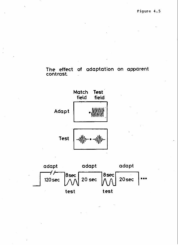
Figure 4.5
The effect of adaptation on apparent contrast
Match Test field field
Adapt ·M_
Test +·+-
adapt adapt
Fsec 8sec 8sec 20sec
test test
adapt
20sec •••

Figure 4.6
The effect of adaptation on apparent contrast matches. I
I
1
... e = unadapted en •=adapted c I L.. ... c 0 u I Cl c ... ·1 1 c _,_,. L.. Cl
.J:. u ... c ·03 ~ adapting
contrast
·03 ·1
Test grating contrast Matc;h and test Adapting grating gratmgs 3 cldeg
3Cldeg r-- _.;. __ ~ fl j r-------~x: 'r 0 ~ x: ·':f
:4~r;~~ols :· : y: o•] a.:.---- - t: (2oseg .. ______ .. 0 contrast •·56
300Cd/m21 MDP3

CHAPTER 4: SUPRA-THRESHOLD EFFECTS .~ge ~5
Thresholds for detection were measured by the method of forced choice (82i
correct 2AFC), shown as white arrows, and by the method of adjustment, shown as
black arrows. The presence of the noise raised the forced-choice threshold
fivefold, from .004 to .02, approximately, for.both observers. DP's
~ethod-of-adjustment thresholds were approximately twic~ as high as RH 1s,
despite their very similar forced-choice thresholds. The possibility of this
sort of criterion difference was an important reason for using forced-choice ~s
the primary method of threshold measurement.
The vertical bars indicate z1 standard deviation about the mean log
contrast of 2 to 8 settings. Where the bars are absent they were smaller than
the plotted symbol. When the test grating was below threshold, and therefore
invisible, the match contrasts were all below threshold. All below-threshold
match contrasts were replaced with the method-of-adjustment-threshold contrast
before calculation of the mean and standard deviation.
The sharp transition from matches with zero contrast to veridical matches
was described by Georgeson and Sullivan (1975) for apparent contrast matches of
gratings of unequal frequencies, and at unequal luminances. On matching
apparent contrasts of unequal frequency they said,
"The observers had some difficulty in making these matches because high frequency gratings seem to have high contrast as soon as they are above threshold. This is a paradox mentioned earlier: at threshold a high frequency grating is barely visible, yet may appear to be of higher contrast than the standard, which is easy to see."
THE EFFECT OF ADAPTATION ON APPARENT CONTRAST
This experiment is essentially a replication of one done by Blakemore,
Muncey, and Ridley (1971), but using the same stimuli as in the noise-masking
experiment: brief grating patches. Blakemore et al. used continuously present
CHAPTE.R 4: SUPRA-THRESHOLD EFFECTS Page t26
half-field gratings.
Method
Figure 4.5 illustrates the paradigm. The observer adapted to a grating in ~he test field with a contrast of .56 for two minutes. Then test and match gratings were presented repetitively for eight seconds. Each presentation of the gratings had the same brief temporal envelope as has been used up to now. During this period the observer was allowed to adjust the contrast of the match grating. When the observer was satisfied with the match he indicated the fact by pressing a button, and the computer recorded the match contrast, and then put up a new, randomly selected test contrast. The observer was allowed to take as long as he liked to make his match, but after every 8 seconds of matching, the adapting grating was returned to the test field to "top up" adaptation for another 20 seconds. After top-up the matching process was resumed automatically from where it was before the interruption. As before, the log contrast of a match grating was proportional to the position of the ten-turn potentiometer which th~ observer controlled, plus a random offset which was changed after each match.
Results
Figure 4.6 plots match contrast as a function of test contrast, in
unadapted (shown as filled circles) and in the adapted state (shown as filled
triangles). The unadapted data were collected in exactly the same way as the
adapted data, except the adapting contrast was zero. Each point is the
geometric mean of four settings. The standard deviation of the settings is
approximately the diameter of a filled circle, except for the leftmost point
which is a half of a standard deviation above the line. The lines were fitted
by eye.
Despite the different sti~uli and conditions used in this experiment, the
results are very similar to those of Blakemore et al. Figure 4.6, as-well as
their results, shows that, in the adapted state, the log of match contrast is
proportional to the log of test contrast: the points all fall on a straight
line connecting threshold of match and test to unity contrast of match and
test.

CHAPTER 4: SUPRA-THRESHOLD EFFECTS ~ge ~7
We have seen that noise masking and contrast adaptation produce very
similar effects on contrast discrimination: discrimination with a sub-threshold
pedestal exhibits facilitation, and discrimination with a suprathreshold
pedestal is una~fected. This raised the possibility that noise masking and
contrast adaptation had a similar mode of action. However, as we have just
seen, suprathreshold matches of apparent contrast were reduced by adaptation
and unaffected by noise masking.
CONCLUSIONS
Effects of luminance noise were compared with the effects of contrast
adaptation. Noise masking elevates the threshold for detection.without
affecting suprathreshold contrast discrimination or apparent contrast.
Contrast adaptation reduces the apparent contrast of all contrasts without
affecting suprathreshold contrast discrimination. Thus they seem to be
distinct phenomena.
The similarity of the effects of noise and contrast adaptation on contrast
discrimination raises the possibility that contrast adaptation elevates
threshold by increasing the observer's equivalent noise; Attempts to measure
the observer's equivalent noise after contrast adaptation gave inconsistent
results and are therefore not reported.
This Chapter's finding that near-threshold phenomena scale with threshold,
combined with Chapter 2's evidence of proportionality of squared threshold to
effective noise level, implies that near-threshold phenomena are unaffected by
proportional scaling of squared. contrast and effective noise level.· Stated
another way, these near-threshold phenomena are not affected by changing the
amplitude of the effective stimulus. The theoretical consequences of this will

CHA Pl'ER 4: SUPRA-THRESHOLD EFFECTS Page T28
be discussed in Chapter 5.
CHAPTER 5
UNCERTAINTY IN VISUAL DETECTION

CHAPTER 5: VISUAL UNCERTAINTY Page 129
UNCERTAINTY IN VISUAL DETECTION
ABSTRACT
We have seen that squared threshold is proportional to the effective noise level. this chapter seeks to incorporate this resul~ into existing explanations of visual detection which succesfully account for other aspects of visual detection. In particular, the standard form of the "probability
summation model.successfully predicts summation effects- the increased detectability of extended patterns - from the steepness of the psychometric function for detection, and the "nonlinear transducer" model predicts contrast-discrimination performance also from the steepness of the psychometric function for detection. Neither of these models provides a satisfactory account of detection in luminance noise.
In detecting a signal an observer usually has two types of information available to him: what is presented during the trial, i.e. the stimulus, and the instructions and practice (often with feedback) he has received before the trial, i.e. prior information. Host attempts to understand visual detection have quite naturally emphasized the role of the stimulus and neglected the role of prior information. This chapter will consider the hypothesis that the observer is intrinsically uncertain, that is, that the observer is unable to make full use of prior information about the identity of the signal. Except for this limitation it is assumed the observer uses all information available in the id~al way. oin order to make quantitative predictions it is nece·ssary to make two simplifying assumptions (orthogonality and equal-detectability of "expected signals", and whiteness of effective noise) which yield the channel-uncertainty model.
The channel-uncertainty model predicts proportionality of squared threshold to effective noise level. It is known that this model can account for the steepness of the psychometic function, and that it is a "nonlinear transducer" model and,a "probability summation" model in the most general sense of each term. It will be shown that the predictions of the channel uncertainty model do not differ sufficiently from the standard versions of probability summation and the nonlinear transducer models, in their intended areas of application, to be distinguished by existing experimental results. Thus the uncertainty hypothesis would seem to offer a parsimonious explanation of many aspects of visual detection.
Appendix 6 reports the results of a direct test ofthe uncertainty hypothesis. When the signal could appear at any of ten-thousand possible times and places over 20° and 2000 msec the observer's threshold was only 1.5-times higher than when the signal appeared at a fixed time and place on every trial. Clearly the observer made little use of exact information about the signal identity when it was provided, confirming the uncertainty hypothesis.

CHAPTER 5: VISUAL UNCERTAINTY Page 130
INTRODUCTION
Chapter 2 showed that quantum efficiency has two components, transduction
efficiency and calculation efficiency, and found that the transduction
efficiency of human observers shows little variation over a wide range of
conditions. This chapter is concerned exclusively with calculation efficiency. ·
·It is assumed that the observer's equivalent noise has already been determined
and referred to the visual field so that we may now ask how the observer makes
decisions about that noisy effective stimulus (i.e. the contrast function of
the actual stimulus, which may be noisy, plus·the observer's equivalent noise).
REVIEW
Attempts to model human detection performance quite naturally first.
consider the ideal observer of a signal known exactly. For example Rose
(1942,1948) and de vries's (1943) fluctuation theory assumed that the observer
would count photons in the area of the disc to be detected, and ignore the rest
of the field. This is only possible if the size and location of the pOssible
signal are known in advance.
d' expresses performance as the signal-to-noise ratio that would be
required by an ideal observer (Tanner and Birdsall 1958) .1 Assuming an tmknown,
but constant noise spectral density, n2 , added to a known signal, the
signal-to-noise ratio, s/n; is proportional to signal contrast (see the
Introduction of Chapter 2). If the human observer acted like the ideal, d'
would be proportional to signal contrast.
1 As noted earlier, this definition of d' is convenient in that it makes no assumptions about the observer. This chapter will refer to many works that used other definitions, however we will mostly be considering situations in which the definitions are numerically equal, so footnotes will appear only when the distinction matters.

CHAPTER 5: VISUAL UNCERTAINTY Page 131 REVIEW
Tanner and Swets (195~) found that both yes-no and
four-alternative-forced-choice methods yielded similar estimates of d' for
detection of a. small spot on a uniform background. They found d' was not
proportional to signal contrast. Instead they found d' proportional to
approximately the third power of signal contrast. This result seems to be .,
general: d' is proportional to the signal contrast raised to a power greater
than 1. Tanner (1961) and Nachmias and Kocher (1970) confirmed this relation
for detection of spots 2 , and they also cite Blackwell's (1963) conclusion that
the data reported in Blackwell (1~6) indicate that d' rises as a power of the
signal contrast greater than one. Nachmias and Sansbury (197~> and Foley and
Legge (1981) extended it to detection of sinusoidal gratings.
Tanner (1961) suggested that the ideal-detection-of-a-signal-known-exactly
model of human performance might be wrong in assuming exact lmowledge of the
signal:
"An examination of our procedure indicates there might be uncertainty both as to the time and location of the signal presentation. The uncer-tainty may be introduced at a central rather than retinal level, suggesting that one should not try to account for nonlinearities at the level of the end-organ, to the exclusion of central hypotheses."
Tanner noted that an ideal observer with uncertainty as to the signal could
have the steep psychometric functions (i.e. d'acck, k>1) observed·
experimentally. Nachmias and Kocher (1970) noted that too, and the additional
fact that their steep ROC curves might also be explained by signal uncertainty.
Cohn (1981) has shown, by simulation, that uncertainty would reduce
quantum efficiency', and noted that this would help explain why our quantum
2 In rating scale experiments each point on the ROC curve yields a value for d' (by the definition we are using). Nachmias and Kocher (1970) calculated d' for the interpolated point with a 50S hit rate.

CHAPTER 5: VISUAt UNCERTAINTY REVIEW
Page 132
efficiency is lower than the estimates of photon absorption (Barlow 1977).
3 This is what Cohn meant. He said uncertainty would "cause psychophysical estimates of quantum efficiency to be too low," but he was using a peculiar definition of quantum efficiency: "the fraction of available photons used in the task". This is meaningful as a parameter in his simple model (used in his simulations) but it is not at all clear what this would mean for something as complex as a human observer. A related point was discussed at the end of the Introduction to Chapter 2.

Stimulus
+ Equival~r.t
Noise
CHANNEL-UNCEBTAINTY MODEL
Peak
Detector
Figure 5.1
>

CHAPTER 5: VISUAL UNCERTAINTY THE CHANNEL-UNCERTAINTY MODEL
THE CHANNEL-UNCERTAINTY HODEL
Theoretical background
Page 133
Even the earliest papers on signal detection theory realized that it would often be unreasonable to assume exact knowledge of the signal to be detected. One of the alternative assumptions they considered was detection of one of H orthogonal signals. Peterson, Birdsall, and Fox (1954) showed that the ideal detector of one of many possible signals' would evaluate the likelihood of each signal and add the likelihoods to obtain the overall likelihood of a signal presence. Unfortunately the resulting equations are difficult to manipu;tate and Peterson et al. were only able to provide an approximate solution for the ideal's performance as a function of the number (M) and strength (i.e. the signal-to-noise ratio, s/n 5 ) of the signals:
2 ( d ') 2
:s ln ( 1 - ~ + ~ ( s/n > )
Nolte and Jaarsma (1967) solved the original equations numerically and published receiver operating characteristic (ROC) curves for several values of Hand s/n. They found that Peterson et al.'s approximation was accurate when s/n was less than 1, and very inaccurate when s/n was as large as 4. The interesting cases for the purposes of this chapter turn out to have large values of M (i.e. high uncertainty). When M is greater than 100 the approximation is inaccurate for values of d' greater than 0.5. Human psychophysical performance can be measured-with reasonable accuracy and effort only over the range of d' extending from approximately 0.1 to 2, and the Peterson et al. approximation is inaccurate over most of this range. Nolte and Jaarsma's solutions are accurate but their paper could only include solutions for a modest number of pairs of values of M and s/n. Fortunately there is now a shortcut to the heroics of the direct solution which Nolte and Jaarsma undertook.
Nolte and Jaarsma also calculated the performance of a simple channel-uncertainty model which they called a "disjunctive receiver" (after Wainstein and Zubakov 1962). This receiver has a channel for each possible signal. Each channel· evaluates the cross-correlation (i.e. integrated product) of the input (i.e. noise and perhaps a signal) with one of the possible signals. It is called a "disjunctive receiver" because each channel then applies a criterion to the cross-correlation and the receiver says "yes" if any channel exceeded criterion. The ROC curves
' assumed orthogonal, equally-detectable, and added to a background of Gaussian white noise. Given the other two assumptions, equal-detectability is equivalent to assuming the signals have equal contrast energy.
5 The notation used by signal-detectability theorists has evolved much since Peterson, Birdsall, and Fox (1954). ~notation follows Tanner and Birdsall (1958) except for signal energy (my s =their E) and noise power spectral density (my n2:their N
012k where k is the dimensionality of the noise). Thus
the signal-to-noise ratio was represented as ld 1 by Peterson et al., as 1(2E5tN0) by Tanner and Birdsall, and as s/n by me.

CHAPTER 5: VISUAL UNCERTAINTY Page 134 THE CHANNEL-UNCERTAINTY HODEL
Nolte and Jaarsma plotted for this .sub-optimal receiver are virtually identical (but not greater than) those of the ideal. The rest of this chapter will consider only a channel-uncertainty model which is equivalent to the disjunctive receiver for the yes-no detection paradigms Nolte and Jaarsma considered, but which will also behave sensibly in tasks such as contrast discrimination which we lmow human observers are capable of.
Following common practice it will be called a "channel uncertainty" model. However, the reader should be warned that these channels bear little relation to "spatial-frequency channels". One "spatial-frequency channel" could provide many cross-correlations (during the course of a psychophysical presentation), each of which would be attributed to a different cross-correlation channel in the context of this analysis.
The new model ----
A channel-uncertainty model was described by Wain stein and Zubakov ( 1962).
As mentioned above, Nolte and Jaarsma showed that it performs nearly ideal
detection of uncertain signals. Nachmias and Kocher (1970) proposed it as a
model of visual detection. All these people considered only yes-no and
rating-scale experiments, and their version of the model (i.e. the disjunctive
receiver) cannot cope.with a' forced-choice paradigm. A more general version
will be presented which copes with all the paradigms, and is equivalent to the
older version for the yes-no and rating-scale paradigms.
This new model is illustrated in figure 5. 1. The input is assumed to be a
sum of the stimulus and the observer's equivalent noise. There are a number of
parallel channels, each "expecting" a different signal. Each channel evaluates
the cross-correlation of the input with the signal it is "expecting". For
simplicity the expected signals are assumed to be orthogonal, and the effective
noise is assumed to be Gaussian white noise. The assumptions are needed for
two reasons. Firstly, the ideal has only been worked out for this case.
Secondly, these assumptions imply that the various channels will be
stochastically independent. Without independence the calculation of
performance would be much more difficult, probably ruling out a direct
CHAPTER 5: VISUAL UNCERTAINTY Page 135 THE CHANNEL-UNCERTAINTY MODEL
numerics~ solution, and requiring Monte Carlo techniques. The orthogonality
requirement would be satisfied by, for example, expected signals that do not
·overlap in space, or do not overlap in time, or that do not share any spatial
frequencies. Each channel produces a single value for each stimulus interval.
~1 these values go to the peak detector whi~h passes only the largest one.
Finally, the decision maker on the right receives the peak value for each
stimulus interval. In two-alternative-forced-choice the decision maker will
choose the interval which resulted in the larger peak value.
The assumption that the effective noise is white is plausible; Chapter 2's
estimates of the observer's equivalent noise sh,owed little -dependence on test
frequency, indicating that the equivalent noise is not far from being white.•
The orthogonality assumption is not plausible, but I believe it is a reasonable .. - -... - .
simplification which may not seriously affect the solution. Imagine an array
of visual neurons implementing the model. If the array is dense the receptive
fields will overlap, and if it is very dense the receptive fields will not be
orthogonal; their responses to white noise will be correlated. However the
response of a cell correlated to its two neighbors will tend to be intermediate
between their responses and thus rarely if ever provide the peak response,
which is all that matters to the peak detector.
It is important to realize that the uncertainty may be over time.
Returning to the visual neurons analogy, each neuron's output will vary over
the course of the psychophysical presentation. If the cell is linear then
several samples, separated sufficiently in time to ·be uncorrelated, would each
1 Of course, since the effective noise is a sum of the equivalent and actual noises, it could be made to have almost any spectrum. However this chapter will only consider experiments which used white luminance noise, or none at all.
CHAPTER 5: VISUAL UNCERTAINTY Page 136 THE CHANNEL-UNCERTAINTY MODEL
be a cross-correlation of the input with a spatia-temporal weighting function, 1
and each of the weighting functions (which are_ delayed ,co.pies of one another)
would correspond to an "expected signal" in the theoretical developnent. 7 .
The .intent of this chapter is to explore the consequences of the
Uncertainty hypothesis. The simplifying assumptions of equal detectability,
orthogonality, and white effective noise which lead to the channel-uncertainty
~" model are needed to make the calculations feasible, and desirable in that they . I
yield a model with only one degree of freedom: the degree of uncertainty, M. 1
For ease of presentation only two-alternative-forced-choice contrast
detection and discrimination of sinusoidal gratings wil~ be examined •. In such
experiments the grating is presented at one contrast in the first interval, and
at another in the second interval. The observer is asked to say which interval
had higher contrast, and one can determine his proportion correct, P(C). That
task is contrast discrimination. When the lower of the two contrasts is zero
it is called contrast detection. Parallel existing results for other paradigms
,~ and signals will be cited where appropriate.
)
'
7 While it seems unlikely that a real peak detector would wait out the necessary delays to ensure that the successive values are uncorrelated, I suspect that the peak of samples taken at the maximum rate at which the samples would still be uncorrelated, would be similar to the peak over the continuous function.
• However the comparisons with human performance presented here will allow a second degree of freedom: the s~ctral density of the observer's equivalent noise. Chapter 2 showed that neritic 1 is an estimate of the observer's equivalent noise, but this measuremen@ was not available for the data considered here.

CHAPTER 5: . VISUAL UNCERTAINTY THE CHANNEL-UNCERTAINTY MODEL
1. CONTRAST DETECTION
1a. Human
Figure 5. 2 shows Nachnias and Sansbury's ( 1974) results for human
Page 137
performance at contras~ detection. The abscissa is a logarithmic scale showing
contrast of the grating to be detected, and the ordinate on the right shows the
proportion of correct responses. The ordinate on the left is a logarithmic
scale of d' '. The scale of the proportion-correct ordinate is determined by
the logarithmic ,scale of ·the d' ·ordinate. Nachmias and Sansbury fit their data
by the solid straight line with slope 2.9. It provides a good fit. For a
second observer they reported a slope of 2. 2. Thus, for bqth observers d' was
proportional to the contrast raised to a power greater than 1.
Some readers may be more familiar- with the weibull (1951) function
suggested by Quick (1974) to describe the psychometric function:
.. -c.£ >B P(C)=1-.5e c. 82
A maximun likelihood fit 10 by the Weibull function is shown too, as a dashed
curve, but it is almost entirely covered by the solid line because, in these
coordinates, the Weibull function produces a nearly straight line with a slope
of approximately 0. 83B. 11
' d' is defined as the signal-to-noise ratio required by an ideal observer to perform as well as the observer under study (Tanner and Birdsall, 1958), but in the experiments reported here the signal was non-random, so d' is just 12 times the normal deviate corresponding to the proportion correct:
d'=l2 t-1{P(C)}.
10 The maximllll likelihood f1 t was made by Watson's ( 1979) computer program, QUICK.

Detection of 9 c/deg Figure 5. 2
10 After Nachmias and Sansbury ( 1974)
slope= 2.9 I .999
-·- - {3=3.65 .99
.90
.80
.76 · . .......
.70 u Q) ~
~
0 u
.60 c:
d' 0 ....... ._ 0 a. 0
.55 ~
a..
J .53
.51
160 .trials/point
Contrast

CHAPTER 5: VISUAL UNCERTAINTY THE CHANNEL-UNCERTAINTY MODEL
1b. Channel-uncertainty model
Theory
Page 138
By assumption each channel evaluates the cross-correlation of the input with some function, in a sense the signal it is expecting. It is assumed that signals are orthogonal and have equal energy and that the noise is white and Gaussian. This implies that all channels produce values which are uncorrelated with equal variance, and with equal mean response to its "expected" signal. For convenience the output values are measured in units of the common standard deviation, so a channel responding to noise alone has probability, t(>.), of not exceeding a value >., where t(>.) is the cumulative normal integral:
2 t(>.)= - 1-- 1>. e-t 12dt.
1(2w) _ ..
A channel responding to its "expected" signal as well as the noise has probability t(>. - s/n) of not exceeding >..
The probability that the peak value will exceed ). in the absence of a signal is:
The probability that the peak value will exceed >. when the signal is presented is:
P(A I SN)= 1-tM-i (>.) tC>.-s/n) •
These equations parameterize the .ROC curve and have been plotted by Nolte and Jaarsma. The proportion correct in 2-alternative forced choice (2AFC) is the probability that the peak in the signal interval will exceed the peak in the other interval and is given by the area under the ROC curve (e.g. see Green and Swets 1966):
>.=+OIJ P(C):J P(A!SN) dP(A!N).
>.=-OIJ Substituting our expressions for P(AIN) and P(A!SN) yields:
f(C)= 1 - 1:: t(>.-s/n) t 2M-2(>.) ~:(>.) d>..
11 The Weibull function was a maximum likelihood fit to the data. The line was Nachmias and Sansbury's least-square error fit. A maximun likelihood fit of a Weibull function to a straight line w1 th slope k (i.e. log d' x k log c) has a B=k/. 83.

CHAPTER 5: VISUAL UNCERTAINTY THE CHANNEL-UNCERTAINTY MODEL
Discussion
Page 139
Figures 5. 3a and 5. 3b show the psychometric functions resulting from this
equation. 12 The abscissa is the signal-to-noise ratio, s/n, and the ordinate is
d' 13 • Figure 5.3a has log-log coordinates. Figure 5.3b has linear-linear
coordinates. Proportion correct is also indicated, on a scale at the right.
The functions are shown for values of M ranging from 1 to 10, 000. Increasing M
pushes the curve to greater s/n and greater steepness. The curves are nearly
straight in log-log coordinates. The dashed curve is Peterson et al.'s
approximation for M=1 00, and is obviously inaccurate for these values. Note
that large changes in M, the number of expected signals, are required to
produce a small change in slope. Nachmias and Sansbury's data in figure 5.2
would be well fit by a channel-uncertainty model with about 1000 expected
signals. Their other observer had a shallower psychometric function
(i.e. slope of 2.2) which would be well fit with about 50 expected signals.
Tanner ( 1961) concluded that about 100 e~pected signals would account for the
steep psychometric function for d~tection of a light increment. The large
range of these estimates of the number of expected signals reflects the large
1z The integral was evaluated by numerical integration. The cumulative normal ' functi~, t(>.), was approximated by a polynomial with an error of less than
7. 5x1 0 (Abramowitz and Stegun, 1964, page 932, eq. 26. 2. 17). It was difficult to check accuracy because this calculation has never been made before. For the case M=1, d' did equal s/n, as it should. The d' values based on P(C) agree with Nolte and Jaarsma's d' values based on the negative diagonal intercept, but this is not a perfect test because these two values need agree only when the ROC curve has unity slope, which these do not.
13 d' is still calculated as 12 times the normal deviate corresponding to the proportion correct: the signal-to-noise ratio that an ideal observer (that knew the signal exactly) would require to equal the performance of the observer ---under study. This is because the experiment was such as to allow an ideal observer to obtain exact knowledge of the signal, but the uncertainty model, by assumption does not use this information. If the signal actually were one of M orthogonal equal-energy signals then d' would be nearly equal to the s/n, because the channel-uncertainty model is nearly ideal in that situation.

Detection of a known signal by
10 a channel-uncertainty model Figure s · 3a
--=exact solutions -- -=Peterson et al approximation
for M= 100 .999 .99
.90
.80 .-0
.76 Q) },..
~
.70 0 u c 0 --.-
.60 ~
0 0.
d' 0 ~
a.. .55
.51
.01._ ______________ ._ ______________ ~
.I 10
s/n
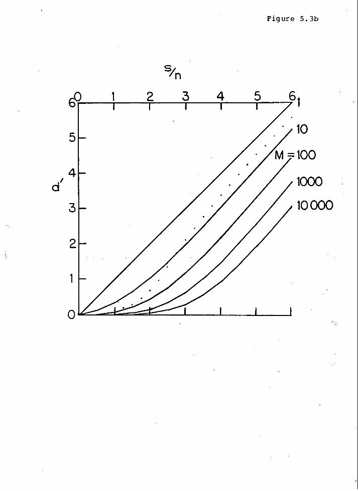
Figure 5.3b
1000
10000
CHAPTER 5: VISUAL UNCERTAINTY Page 140 THE CHANNEL-UNCERTAINTY HODEL
range of estimates of psychometric steepness and the fact that the model's
steepness is proportional to the log of H.
These nearly linear curves suggest that we might characterize each curve
by two numbers indicating its rog-log slope, k, and signal-to-noise ratio,
( s/n). 71 , at the point where d '=1 (and P(C):76~). These two values determine a
line in our double logarithmic coordinates:
d'= {(s/n) }k ( s/n) • 7 6
log d'= k log{ (s/n) } TSTri) .7 6
Figure 5. 4a shows k versus H1 a.. The slope, k, increases approximately in
proportion to the logarithm of H. A second ordinate (on the right) shows 8,
the Weibull index of psychometric steepness, which is 8=k/. 83 (see the previous
footnote). Figure 5. 4b shows ( s/n). 7 6 as a function of H.
2. EFFECTS OF NOISE MASKING ---- -- --- ---2a. Human
Preceding chapters have presented evidence that squared threshold contrast
is proportional to the effective noise level, which is the sum of the
observer's equivalent noise and any actual luminance noise.
la. The fitting procedure took advantage of the fact that the Weibull function is virtually straight in these coordinates with slope 0.838 (e.g. see figure 5. 2). Proportions correct ·were calculated for the channel-uncertainty model. Then a maximiln likelihood f1 t was made with the Weibull function to "dummy.; data with 1000 "trials" at 20 signal-to-noise ratios and proportions correct as calculated for the model. A x2 statistic indicated that the f1 tted function was an excellent representation of the (dummy) data (Watson 1979). Finally the slope was taken as 0.838.

Detection of' a known signal Figure 5.
b~ a channel-uncertaint~ model
Figure 5.4a
5
..X. 4 en 3 (3 en 4> 2 c a. 4> 1 4>
+"'
0 V)
1 10 100 . Uncertainty M
Figure 5. 4b
5
4
~ "" :-...c en 3 ~
::2 0 2 .s::. en 4> L.
.s::. 1- 1
o~--~--~----~--~ 1 10 100 1000 10,000

CHAPTER 5: VISUAL UNCERTAINTY Page 141 THE CHANNEL-UNCERTAINTY MODEL
Figure 5. 5 shows human psychometric functions for detection of a 1 c/deg
grating without noise (on the left) and in the presence of dynamic,
one-dimensional white noise (on the right). The solid curves are maximum
likelihood fits (of the Weibull function). The vertical bars are 95~
~onfidence intervals based on binomial statistics applied to the raw data at
each contrast. The presence of the noise increased the contrast required for
any level of performance by nearly an order of magnitude, but the shape of the
psychometric function is hardly changed (in these coordinates). The in-noise
curve on the right is slightly steeper, but not significantly so.
Griffiths and Nagaraj a ( 1963) reported that their psychometric functions
(proportion correct versus 16g contrast) had the same (steep) shape for
detection of a disc with or without two-dimensional, dynamic,· white noise.
Cohn ( 1976) obtained steep psychometric functions ( d' a:ck, k>1) for detection of
a luminance increment with and without dynamic (zero-dimensional) noise. All
reported psychometric functions in (continuously on) dynamic noise indicate a
psychometric function steeper than d' a:c.
However in static noise the situation is unclear. Henning, Hertz, and
Hinton ( 1981) report steep psychom~tric functions for detection of gratings in
static one-dimensional noise. Burgess, Wagner, Jennings, and Barlow (1981b)
reported the same, but with static two-dimensional noise. Barlow (1978) and
Burgess and Barlow ( 1981) report proportionality of d' to contrast for
detection of large increments on a static dot display. This would indicate
that (static) dot displays are the only exception, but Burgess (personal
communication) finds that under some conditions he obtains unit slope with
two-dimensional static noise. A consistent finding of a unit-slope
psychometric function (d'a:c) could be interpreted as evidence that the

10
d'
.I
Effect of noise on detection of I c/deg Figure 5 • 5
-- -{]=3.6 -- -fJ= 4.7
I
I
I
I
I
I I
I I
2 to 93 trials/point
no noise 500 trials
.01
Contrast
with noise 500 trials
Signal ·1 c/deg
•
. x:4° y:40 t:7oms
40
.I
.999 ·.99
.90
.80
.76
.70
.60
.55
.53
.51
Noise 0-50Hz
.... 0 Q) ~
~
0 (.)
c 0 ·-.... ~
0 a. 0 ~
Q_
CHAPTER 5: VISUAL UNCERTAINTY Page 142 THE CHANNEL-UNCERTAINTY MODEL
observer's intrinsic uncertainty is purely temporal, and thus not detrimental
when detection is limited by static noise. This interpretation is supported by
the high 711·efficiency for detection recently reported by Burgess, Wagner,
Jennings, and Barlow (1981a) for detection of a grating in static
~wo-dtmensional noise.
2b. Channel-uncertainty model
Noise added at the display just increases the effective noise level. The
channel· uncertainty model's performance is unaffected by proportional scaling
of the squared contrast and the effective noise level. So increases in
effective noise level will just shift the psychometric function to higher
contrasts on our logarithmic contrast scale, without changing the function's
shape.
This is an important point of agreement with the human data. Many other
models of human detection assume stochastic processes that cannot be treated as
an equivalent noise at the input, and thus predict very different behavior for
detection with and without noise at the display.
2c. Probability summation
Nachmias (1981) has recently presented a clear analysis of the assumptions
made in the standard form of probability summation calculations. In general,
probability summation means only that - in a yes-no task - an observer will say
"yes" if one or more of many independent events occurs. Nachmias points out
that this includes the channel-uncertainty model. ~wever, two other
assumptions are usually made for analytical conven~nce, and these are not
compatible with the channel-uncertainty model. According to the high-threshold
CHAPTER 5: VISUAL UNCERTAINTY Page 143 THE CHANNEL-UNCERTAINTY HODEL
assumption there are no events in the absence of a signal, and according to the
homogeneity assumption the probability of one or more events depends on signal
contrast in the same way as the probability of any particular event does
(except for a contrast-scale factor).
These events are usually described as a "detector" going into a "detect"
state. Thus the high-threshold-version of probability summation incorporates
noise only as the probability that each individual "detector" will go into a
"detect" state in the presence of a signal. For convenience, every detector's
probability of a "detect" is described by Weibull ( 1951) functions with the
same steepness (homogeneity assumption) Which is substantially steeper than the
cumulative normal. By assumption the detectors never "detect" in the absence
of a signal. 15 Presence of substantial effective noise at input would firstly
increase every detector's probability of going into the "detect" state, even in
the absence of a signal. One could suppose that an internal criterion was
adjusted to reduce the "detect" rate to virtually zero in the absence of a
signal, but the probability of any detector "detecting" would still have become
a cumulative normal (which has a very low index of steepness). Thus noise at
I the input of a standard probability summation model would seriously change its
behavior: violating its assumptions of high-threshold and homogeneity. This is
because the high-threshold assumption is incompatible with the finding that
1 5 This "high threshold" assumption makes the calculati~ns simple but introduces serious theoretical problems (Nachmias 1981). To account for the fact that actual observers do occasionally say "yes" in the absence of a signal it is usually assumed that these "yes"s are due to an independent guessing process. However it has been well established that these "yes"s are not independent (Tanner and Swets 1954, Nachmias 1981) contradicting the high-threshold assumption. On this basis alone, the fact that the channel-uncertainty model does not incorporate the high-threshold assumption makes it a more plausible formulation of probability summation.

CHAPTER 5: VISUAL UNCERTAINTY Page 144 THE CHANNEL-UNCERTAINTY MODEL
detection is unaffected by proportional increase of squared contrast and
effective noise level.
2d. "Nonlinear transducer" model
Nachmias and Sansb~ry's (1974) "nonlinear transducer" model is not
sufficiently explicit to make a prediction for the effects of noise at the
visual f1eld. They confined themselves to hypothesizing a nonlinear relation
between an "internal effect" and signal contrast. The model amounts to the
hypothesis that d' is a nonlinear function of contrast, which was known aleady,
and Y'lat I call "d' additivity" (explained below), by which they accurately
predicted contrast discrimination performance from the psychometric function
for detection. They pointed out that channel-uncertainty would be one way of
implementing their "nonlinear transducer" model.
Alterna~ively a more literal interpretation of "nonlinear transducer"
would take the decision statistic to be a nonlinear transformation of signal
contrast, to which a Gaussian internal noise is added. Foley and Legge ( 1981)
have used such a model to accurately account for detection and discrimination
data. There is no equivalent input noise for the noise in this model, and. by
Birdsall's theorem (Lasely and Cohn, 1981), in the presence of a substantial
noise at its input the internal noise and the nonlinear transformation would
have no effect on performance, and the psychometric function should have unit
slope (plotted as log d' versus log contrast), contrary to fact.

CHAPTER 5: VISUAL UNCERTAINTY THE CHANNEL-UNCERTAINTY HODEL
~CONTRAST DISCRIMINATION: "d' ADDITIVITY"
Page 145
We can discriminate contrasts that differ by less than the smallest
contrast we can detect. This phenomenon is sometimes called "facilitation".
Nachmias and Sansbury (1974) showed that facilitation may be related to the
steepness of the psychometric function for detection. They showed that they
could predict the d' for discriminating tw contrasts by the difference in d's
for detecting them. I call this finding~ additivity. 1 '
Think of d' as a distance between tw contrasts along a discriminability
continuum. For detection one of the two contrasts is zero. Nachmias and
Sansbury found that these distance add t so that the discriminability of c1 from
c3 equals the sum of the discriminability of c 1 from ~ plus the
discriminability of c 2 from c3
• 11
Foley and Legge (1981) have measured psychometric functions for detection
and discrimination in order to test the d' additivity hypothesis. Their data
were in excellent agreement with d' additivity. Can these data reject the
channel-uncertainty model? The circles in figures 5 •. 6a, 5.6b, and 5.6c
represent proportions correct for observer JHF in detection of spatial
11 The meaning of d' additivity depends on the definition of d'. .I am sticking to the Tanner and Birdsall (1958) definition because it can be measured without assumptions about the observer. We will see that, by this definition, d' additivity is nearly, but not exactly a property of the channel-uncertainty model. Nachmias and Sansbury ( 1974) defined d' as the mean value. of the decision statistic ("internal effect") on a signal and noise presentation minus the mean value on a noise-only presentation, all divided by the standard deviation on a noise-only presentation:
d' = (psN-pN)/aN.
Nachmias (personal communication) has pointed out that by this definition of d', the channel-uncertainty model satisfies d' additivity exactly.
CHAPTER 5: VISUAL UNCERTAINTY Page 146 THE CHANNEL-UNCERTAINTY HODEL
frequencies of .5, 2, and 8 c/deg. Each point represents about 200 to 300 2AFC
trials. In Figure 5.6a error bars are shown for each point indicating the 95~
confidence interval based solely on the binomial distribution. Foley and Legge
( 1981) determined the best values of H and scale factor (between s/n and c) to
fit (by least squares) these data. That fit is shown by the continuous line
running through the circles. As they noted it is a good fit. The squares
represent proportions correct in contrast discrimination. They have been
predicted by d' additivity (the dashed curve), and by the contrast
discrimination performance of the same channel-uncertainty model used to fit
the detection results (the solid curve, explained below). There were no
degrees of freedom in either prediction. These data cannot reject either
hypothesis. The extent to which the channel-uncertainty model fails to satisfy
d' additivity may be too small to distinguisn in a feasible experiment.
17 To write this as an equation let d'(c1,c ) represent the d' for discriminating contrasts c 1 and c2• Speciffcally, they found that
d'(c1,c2 ):d'(O,c2 )-d'(O,c 1)
so we may write
and
d'(O,c2 )=d'(O,c3 )+d'(c2 ,c3 )
Substituting these quantities in the first equation gives
d'(c 1 ,c2 ):d'(c1 ,c3 )-d'(c2 ~c3 )
which is just the claimed d' additivity:
d'(c1,c3):d'(c1,c2 )+d'(c2,c3).
Nachmias and Sansbury examined values of c 1 ranging from 0 up to .0014, where d' (O,c 1 >-2. 4, but they only used one value of c2• However Foley and Legge ( 1981) have used several values of c2 and confirmed d' additivity.

M=296 after Foley and LeggeU98ll .5 Cfdeg
6
o=de~ection of c .999 o=discrimination of c
from .004
3 =channel uncertainty - -=d' additivity · P(Correctl
.95
.90
.76
.60 0 t---....~~_.:_-r-----~o:::...!.,_~-...-------__J.so 0 .006

69- 4 M=285
5 after Fole':J and LeggeU981l 2 Cfdeg
o=detection of c
d/ 4 o=discrimination of c
from .0023
3 =channel uncertainty . - -=d' additiviiy ·
2
1
6
,999
.99
.95
.90
.76
.60 o ~--~
0~..J---__,_.....LL...£.-~--r-----~.so
0 .001 .002 .003 .-004 contrast
P<Correctl
U1 . "' 0"

1
M=2032 Fole\d and , LeggeU981)
6
8 CJdeg O=detection of c .999 o=discrimination of c
from .0031
=chCflnel uncertaint~ - -=d' additivi"hj ·
·.002 contrast
.99
.76·
P(Correct)
l1l . 0\ ()

CHAPfER 5: VISUAL UNCERTAINTY THE CHANNEL-UNCERTAINTY HODEL
3b. Channel-uncertainty model
Theory
Page 147
The contrast discrimination performance of the channel-uncertainty model may be calculated from our formula for P(AISN). Let the two signal strengths to be discriminated be s 1 and s 2• Then
P(AIS 1N)=1-t(l-s 1/n)tH-1(l).
P(AIS2N)=1-t(l-s2/n)tM-1(l).
These describe an ROC curve, and P(C) is given by the area enclosed. A=+GD
P(C)=/ P(AIS1N) dP(AIS~) . l:-ao
Discussion
Figures 5.6 and 5.7 plot d' as a function of the signal-to-noise ratio in
the "signal" interval, ( s 1tn), for several values of the signal-to-noise ratio
in the "noise" interval, (s2;n). As before d' is 12 times the normal deviate
corresponding to P( C) • The uncertainty, M, is 1 in 5. 7a, 10 in 5. 7b, 100 in
5.7c, 1000 in 5.7d, and 10000 in 5.7e. The prediction of d' additivity is
indicated by the dashed curves which are just vertical translations of the
detection curve, ie.
The deviations from d' additivity are quite small.
~ CONTRAST DISCRIMINATION: FACILITATION
3'a. Human
Thus far we have seen that the channel-uncertain model has two properties
of human observers: firstly, its psychometric function for detection is well

--=channel uncertai nt':J - -·=d additivi-ty ·
M=1
/ /
/
/ /
/ / /
/
/ /
/ / /
/ /
/ /
/ /
/
/ /
/ /
/
/
/ /
/
/ /
/ /
/ /
/ /
/ /
/ /
"/ /
/
Figure 5. 7a
2
4
5
/

Figure 5. 7b
5 --=cha'lnel uncertaint\j
4 - -=c1 additivity ·
d' M=10
3
2
1
0 - / / / -/ / / / ...., / - / - / /
/ / / / /
/ / .,.,.,... / -- / / / /
/ / .,. .,.,.,...
/ _.-/
/ /
/ .../ --

Figure 5. 7c
=chcrlnel uncertaint'=J - --=d' actditivity ·
M=100
0 - / / -· _.-
/ / /
/ / ..---- /
/ / / /
/ / /
~ - / ---- / /
/ ./
/ ~
- -- ..-

Figure 5. 7d
=cha'lnel uncertainty - -=a additivity ·
M=1000 ~/n = 0
0 / / / .......
- - / - --- / /
/ / ----- - / /
/ .,.,... -- - -

Figure 5.7e
SVn
~--~,--~~~3--~4--~---
5 =cha1nel uncertaint':J - -=d' adc:Jitivii":J ·
4 M =10000
- - - - / / /
/ / -- / - - - - - - -/
/ /
/ ---- - -- - - - -

CHAPTER 5: VISUAL UNCERTAINTY THE CHANNEL-UNCERTAINTY MODEL
approximated as d'«ck, where k is greater than one (assuming M>1), and
secondly, within experimental error, it obeys d' additivity.
Page 148
Nachmias and Sansbury also reported the contrast difference threshold as a
function of pedestal contrast. Threshold was taken to be the contrast
difference required for some arbitrary percent correct. The contrast
difference first fell with increasing pedestal contrast, and then rose. They
explained that facilitation was related to the steepness of the psychometric
function by d' additivity 18 (though they did not call it "d' additivity").
Following their argument we can predict the relation between the contrast
difference threshold and the pedestal contrast, using just d' additivity and
the steepness of the psychometric function for detection: 11
(~~P)={(~ )k + 1}1/k _ (~ ). p p p
This equation has been graphed in figure 5. 8 for various values of k. Note
that the relation between (~cp) and (~ ) depends only on k. It is c c p p
independent of the threshold criterion, p=P(C), so even method-of-adjustment
thresholds could be fit by the relation to obtain an estimate of k.
Figure 5.9a (replotted from figure 4.1) shows (~c• 12 ) and . c •• 2
c (0 ) for contrast discrimination in various noise levels: zero for the el2
triangles, .8x10-6 sec deg2 for the circles, and 8.4x10⁻⁶ sec deg2 for the X's.
Psychometric functions were not available to allow an exact prediction, but it
may be seen that the relation is independent of the noise level. Since the
near-threshold phenomenon scales with threshold contrast, and Chapter 2 showed
11 Nachmias and Sansbury's ( 1974) different definition of d' does not affect how they calculated d' from human performance, only how they would calculate d' from models, so their statements about human performance do not need to be modified in order to be consistent with our usage.

Figure 5.8
Contrast discrimination as predicted by a additivity
1 -1 k=1 1
o_ u
CP- IJk 1·5
<J ·3 ~Cp(~k.~k)-C 2 +J (/)
0 2·5 '-+J
c: ·1 3 ·1 0 u
Q) 3·5
u '- 4 Q) '- ·03 4·5 Q) .... ....
k= oO Cl 5
·01 ·01 Contrast

0.. u CF-<J 3 ...., til 0 '-...., c 1 0 u
·3
0
The effect of norse on contrast discrimination.
Noise spectral density
x • 9 10-e sec deg2
o • •9 1o·e sec deg2 6 • no noise
-=chalnel ·unceMainty M=1024 - -=d' additivity · k=3
X
·1 I I I
·3 Contrast
D.
§
A
D. ~ 0
0 0 §X 0
X
~ X
X
Signal 4c/deg .x:4• 0
y:4 . t:70ms
300cd/m2
0
@ . 0 0
Noise. 0-50Hz

CHAPTER 5: VISUAL UNCERTAINTY THE CHANNEL-UNCERTAINTY MODEL
Page 149
that squared threshold is proportional to the effective noise level, this
implies that near-threshold.contrast discrimination is unaffected by
proportional .inc;ease of squared contrast and effective noise level.
Note that all the data points for all noise levels are clustered along the
falling curves (explained below) for subthreshold pedestal contrasts
(i.e. c/c_. 82 i 1), and are widely scattered for suprathreshold pedestal I
contrasts (i.e. c/c. 82 > 1). In a similar way the predictions coincide at
11 Let the two contrasts to be discriminated be c and e+Ac, where c is the
"pedestal", and Ac is the contrast difference. d' additivity states that
d'(O,c+Ac)=d'(O,c)+d'(c,c+Ac).
Let A:P be the discrimination threshold, i.e. t.h. e contrast difference Ac for each pedestal c required for proportion correct p, i.e. p:P(C):t(d'/12). And write cp=Ac for the detection threshold when the pedestal c is zero. Acp is defined so ~hat d' (e+Acp,c) is constant and independent of c, so
d' (e+Acp,c)=d' CO+Acp,O)
=d'(c 0) P'
Substituting into the d '-additivity equation we have
d'(O,c+Ac):d'(Q,c)+d'(O,cp)
Now use the psychometric function d' a:ck to substitute for d':
( C+AC ) k:Ck+Ck p p'
Solving for Acp,
Ac =(ck+ck)1/k- c p p
Dividing through by the detection threshold cp leaves the desired result:
(A~P):{(~ )k + l}1/k _ (~ ). p p p
When k is infinite the equation reduces to
cp-c for c<cp Ac :{
p 0 for c>cp.
which is a classical high threshold.
CHAPTER 5: VISUAL UNCERTAINTY Page 150 THE CHANNEL-UNCERTAINTY HODEL
subthreshold pedestal contrasts, and diverge at suprathreshold contrasts (where
no single curve could account for the data).
Recall that the performance of the channel-uncertainty model at contrast
discrimination was calculated and plotted in figure 5.6. It is a simple matter
to read off the contrast thresholds (e.g. where d'=1) for each pedestal
strength. The solid curve in figure 5.9 is the contrast discrimination
threshold for a channel-uncertainty model, where M:1024. As the pedestal is
increased the discrimination threshold falls until the pedestal exceeds the
detection threshold.
For comparison, the approximate slope, k=3, of the psychometri~ function
was read off figure 5. 4a for the 1024-channel observer. We have noted earlier
that the psychometric function is approximately d'c(s/n)k, and that d'
additivity holds within experimental error. The dashed curve represents the
prediction of d' additivity, assuming k=3. The t-.«> functions agree perfectly
up to the threshold for detection. For 1 arger pedestals the threshold for the
channel-uncertainty model remains constant while the threshold based on d'~
additivity and d' cck continues to fall. This difference does not provide
evidence against d' additivity. The psychometric function can only be measured
for modest ~alues of d' and the power law psychometric function may not hold
beyond the measured range of d'.
The agreement among the data from different noise levels for subthreshold
pedestals indicates that discrimination of subthreshold contrasts is unaffected
by proportional change of (squared) contrast and noise level, and does not
depend explicitly on absolute contrast. This is also the region of agreement
with the predictions. This is reasonable: the d'-additivity prediction is
valid over this region only, and the channel-uncertainty model, like the data,

CHAPTER 5: VISUAL UNCERTAINTY Page 151 THE CHANNEL-UNCERTAINTY MODEL
depends only on ratio of signal and noise, not on the absolute level of either.
The tremendous scatter of the points at suprathreshold contrasts shows
that suprathreshold contrast discrimination does depend on absolute contrast.
Figure 5.9b (a copy of 4.1) shows the original data, contrast discrimination
threshold versus pedestal contrast. Note that the discrimination thresholds on~
the falling part of the curves (sub-threshold predestals) are all different at
different noise levels, but are in excellent agreement over the rising part of
the curve (supra-threshold pedestals), showing dependence on absolute contrast,
and independence of noise level. This would seem to be evidence for
signal-dependent noise, which is not a property of the channel-uncertainty
model, though it could be incorporated easily without changing the prediction
for subthreshold contrasts~
4. SUMMATION EFFECTS
4a. Human
Over the past few years there has been some importance attached to studies
of summation, that is, measurements of th~ contrast threshold for sinusoidal
gratings as a function of number of bars· (e.g. Legge 1978b, Robson and Graham
1981), or exposure duration (e.g. Legge 1978, Watson 1979). Over a wide range
in each dimension the contrast threshold falls slightly if the grating is
extended in space or time. Over this range threshold is inve~sely proportional
to the extent raised to a small exponent, usually called the index of
summation. Using the standard probability-summation calculations these studies
and others were able to successfully predict that the index of summation was
equal to 1 /a, the reciprocal of the index a of psychometric steepness.

u <]
·3
·1
·003
The effect of noise on contrast discrimination.
X X f-1 r-------. X
Noise spectral density
x • 9 10~ sec deg2
0 • •9 10-e sec deg2 A • no noise
8 Signal
•4c/dex~ 4o
Noise o-50Hz
• 0
y:4 t:70ms
300cd/m2
l . lthresholds
· for I I I I I I deteyt iop I
·03 ·1 ·3 Pedestal contrast
c
I I I I 1
Ul .
CHAPTER 5: VISUAL UNCERTAINTY THE CHANNEL-UNCERTAINTY MODEL
Page 152
Figure 5.10 shows a psychometric function from Legge (1978) for detection
of a 180 msec 3 c/deg grating. It is well fit by a Weibull function,
s P(c) = 1-eac ,
'.'lith exponent S=2. 44, shown by the dashed curve. The solid curve, also a good
fit, represents a 32-channel unc.ertainty model.
Figure 5.11 showS the thresholds reported by Legge for durations 180 to
3000 msec. He took threshold to be 71S correct. The dashed line shows the
prediction of probability summation, based on the psychometric function we just
saw for the 180 msec duration. That is,
ca:duration-1 /S.
The solid lines connect the predictions of the channel-uncertainty model
assuming the signal stimulated from 1 to 16 of the total of 32 channels
(explained below). Note that up to 1000 msec the predictions are both
reasonably close to the data, though the predictions are somewhat steeper than
the data. The discrepancy is not significant because there is a large variance
associated with estimating the index of steepness of the psychometric function.
The important point is the great similarity in the predictions of these two
forms of probability summation. No one has reported this· fact before.
4b. Channel-uncertainty model
The calculations up to now assumed that only one channel was stimulated by
the signal. Here it will be supposed that as a grating is extended it
stimulates more and more of the channels. Since M was derived from the
psychometric function for the 180 msec condition, it will be assumed that only
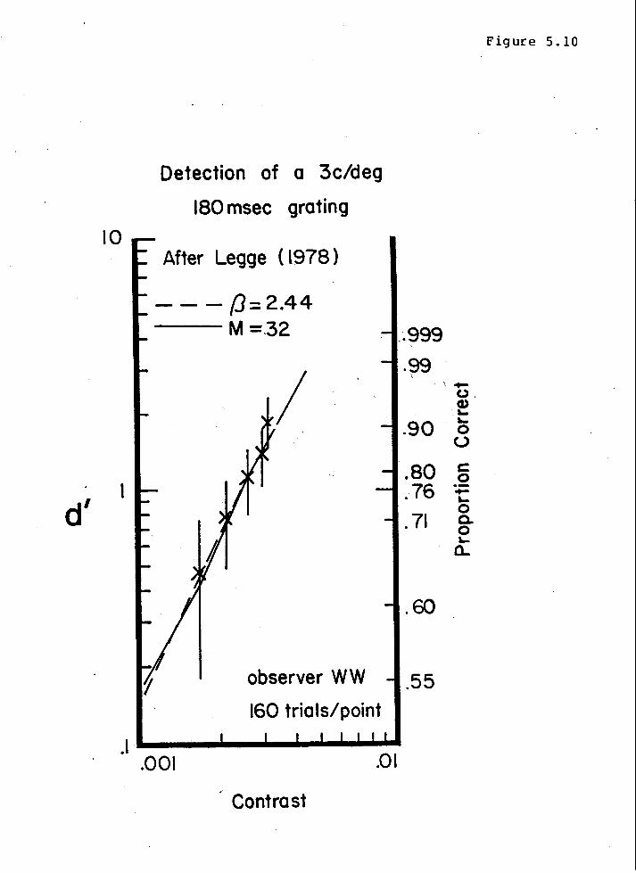
d'
10
Detection of a 3c/deg
180 msec grating
After Legge ( 1978 )
---{]:2.44 ---M=.32 .~999
'/ observer WW
160 trials/point .1 .... _..._...__.._ ......................
. 01 .001
Contrast
.99 '
.90
.80
.76
. 71
.60
.55
\ ... (.), Q) '-'-0
(..)
c 0 ·-... '-0 0.. 0 '-a.
Figure 5.10

-en e -c:: 0 u "0 0 iS ~
.J::,
1-
.01
.001
100
Threshold as a Function of Duration
# of channels stimulated by the grating l ~ I
I I I I I After Legge ( 1978)
probability summation, 0=2.44.
channel uncertainty, M=32
*
I I I 1000
Signal Duration (milliseconds)
I I I I U1 . 10,000

CHAPTER 5: VISUAL UNCERTAINTY THE CHANNEL-UNCERTAINTY MODEL
Page 153
one ch~nnel bears the signal in that condition, and that for longer signal
durations a proportionate number of channels will bear parts of the signal.
Theory
We have simul taneo~ presentation of a signal with N parts, each with signal-to-noise ratio siN (so the total signal-to-noise ratio is s/n, as always). We have
As before
P(AjSN):1 - tM-N(A) tN(A - ~'n)
P(AjN):1 - tM(A).
A:+ao P(C)=/ P (AI SN) dP(Aj N).
A:-ao
Substituting in P(AjSN) and P(AJN) gives
P(C):1- H 1:: t2M-N-1(A) tN(A- ~~n) ~~(A) dA.
Discussion
Figure 5. 11 shows that the prediction of the channel-uncertainty model is
very similar to that of the standard version of probability summation. To test
the generality of this conclusion similar calculations were made for 1024
channels. The psychometric function of this model is well fit by a Weibull
function with s=4.0 (as shown by figure 5.2). The predicted thresholds are
virtually identical for 1 to 64 signal-bearing channels, and differ by less
than a factor of 12 up to 512 signal-bearing channels. Thus the summation
predictions by the high-threshold version of probability summation and by th~_
channel-uncertainty model do not differ appreciably. The similar predictions
by the two models should not be surprising; they are both probability summation
models.
We have seen that the two models are readily distinguished by adding noise

CHAPTER 5: VISUAL UNCERTAINTY Page 154 THE CHANNEL-UNCERTAINTY HODEL
at the input, which defeats the high-threshold assumption. In principle,
summation experiments too could distinguish the two models, but the difference
in the predictions may be too small to measure. 2 0
20 The standard version of probability summation explicitly assumes the psychometric function steepness to be constant (Nachmias, 1981, calls this the "homogeneity" assumption), while as more 'and more of the channel-uncertainty model's channels bear signals its psychometric function becomes more and more shallow, reaching d 1 «C when all its channels bear signals. However my calculations of this effect show that a large proportion of the channels must be stimulated by the signal before B changes much. It would be difficult to obtain a large enough range of signal extent and sufficiently precise estimates of B in order to distinguish the slightly different predictions of the two forms of probability summation. Uncertainty among 1024 channels produces a B of 3. 5 for a one-channel signal. 64 channels must be stimulated for B to drop
'to 2.5. 200 channels must be stimulated forB to drop to 2. Summation experiments have covered ranges of signal extent much less than this, and estimates of B are notoriously variable. For example, Watson (1979) varied signal duration from 100 msec to 800 msec, only an 8:1 range, and reported 52 estimates of B for observer RP with a mean of 4. 7 and a standard deviation of 1. 4. None of the summation studies report the steepness of the psychometric function as a function of signal extent.

CHAPI'ER 5: VISUAL UNCERTAINTY TESTING THE UNCERTAINTY HYPOTHESIS
TESTING THE UNCERTAINTY HYPOTHESIS
Page 155
The uncertainty hypothesis predicts that since the observer makes little
or no use of prior information about signal identity he should perform nearly
as well without it. Appendix 6 presents the results of an experiment which
measured the effect of depriving the observer of the prior information about 0..
signl identity which is usually made available to him. There have been several 1\.
experiments which compared detection of one stimulus with detection of one of
several of disparate stimuli, and found that the experimental uncertainty
caused a small reduction in detectability. For example Cohn and Lasley (1974)
compared detection of a spot at one, or at one of four disparate locations;
Greenhouse and Cohn ( 1978) c.ompared detection of a spot of one, or one of
several colors; Davis and Graham (1979) compared detection of a grating of one,
or one of several spatial frequencies. At first blush these experiments would
seem to be evidence against the uncertainty hypothesis because they indicate
that introducing only a small uncertainty reduces the observer's performance
measureably, implying that the observer ~making use of the information
available in the certainty condition. However, asking an observer to detect
one of several disparate signals may result in an enormous increase in his
uncertainty if he monitors the entire area, hue range, or spatial-frequency
bandwidth that the set of possibilities extend over.
The experiment reported in Appendix 6 _compared detection of a thin <.J-o),
brief (20 msec), bright line at a fixed time and location, with detection of
the same at one of ten-thousand possible contiguous times and places. Thus the
uncertainty condition included all possible, nonoverlapping, signals within an
area 24° wide and a duration 2000 msec long. The threshold in the uncertainty
cond_ition was only a factor of 1.5 higher than in the certainty condition. It

CHAPTER 5: VISUAL UNCERTAINTY TESTING THE UNCERTAINTY HYPOTHESIS
Page 156
is not necessary to believe that the~observer can resolve all ten-thousand
signals; even if he could only resolve signals separated by 100 msec, the
uncertainty was 2000. Thus, as predicted by the uncertainty hypothesis,
drastic reduction in the prior information had little effect on observer
performance.

CHAPrER 5: VISUAL UNCERTAINTY Page 157 CONCLUSIONS
CONCLUSIONS
The channel-uncertainty model behaves as humans do in at least four
respects:
1. The psychometric function is steep (d'~ck, k>1).
2. Detection and discrimination of near-threshold contrasts are unaffected by
proportional increase of squared contrast and effective noise level.
3. d' is additive within experimental error, that is, discriminability of two
contrasts· equals the difference in their detectabilities, so the steepness of
th~ psychometric function for detection implies the existence of facilitation
in discrimination.
4. Summation effects: the small index of summation can be predicted from the
high index of steepness of the psychometric function.
Various theories of visual detection embody idealizations of relations
observed empirically. Over the years study of detection and discrimination has
yielded several simple relations which are analytically convenient and which
give good account of some aspect of detection. These relation accurately
predict summation effects (by probability summation) and contrast
discriminability (by d' additivity) from the psychometric funct~on for
detection. To these relations we may add the fact that detection and
near-threshold discrimination are unaffected by proportional increase of
squared contrast and effective noise level. Past suggestions that uncertainty
may underlie the steepness of the psychometric function and its relation to
discrimination, have been extended here to show that the channel-uncertainty
model exhibits the observed relations (summation effects, d' additivity 21 , and
independence of c2 /n2 ) within experimental accuracy, though not with the
analytic convenience of models which each accounted for only one of the

CHAPTER 5: VISUAL UNCERTAINTY Page 158 CONCLUSIONS
phenomena. Within their intended realms of application the more restricted
models do not seem to be experimentally discriminable from the
channel-uncertainty predictions. Thus d' additivi~ and standard probability
summation should continue to be useful for calculation, even if we accept the
channel uncertainty model as the explanation.
The uncertainty hyp~thesis offers parsimonious explanation of many
characteristics of visual detection. This suggests that human observers do not
use exact knowledge of the signal in contrast detection. This was confirmed by
direct experimental test.
21 Nachmias and Sansbury ( 1974) suggested this might be true, without proving it. Nachmias and Kocher (1970) showed something analogous to d' additivity held for ROC performance of the channel-uncertainty model~

APPENDIX 1: Page 159 CHARACTERIZING VISUAL NOISE
APPENDIX 1
CHARACTERIZING VISUAL NOISE
Perhaps the greatest hurdle in comparing and understanding the experiments
that have studied effects of visual noise 1 is the profuse variety of terms that
-have been used to specify the physical characteristics of the noise.
Luminance noise is random fluctuation of luninance over time or space, or
both. By "random" I mean unpredictable by even an ideal observer. This will
allow comparison of actual observer performance with that of an ideal observer.
In terms of this definition an image presented repetitively and predictably to
an observer is not random, and hence is not noise, no matter how it was made.
While luninous stimulation always extends in two spatial dimensions as
well as time, luminance noise will be described only in its dimensions of
random variation. Thus we will speak of "zero-", "one-", and "two-dimensional"
noise, to indicate the number of spatial dimensions over which the noise varies
randomly. Noise that fluctuates randomly over time will be called "dynamic",
otherwise it will be called "static". Note that this definition allows for a
"static" noise pattern to be faded on and off.
A few exanples may help. A grainy photograph (seen for the first time)
1 This usage is common now, but relatively new. Higgins and Perrin ( 1958) protested its arrival,
"Strenuous objections have been raised to the extension of the term 'noise' from the field of acoustics to the fields of photography and optics, but the use of the term in commll'lication theory to mean an tmwanted signal of any description seems to be firmly established. Any extension of the term 'noise' to the photographic or visual aspects of granularity is still objectionable."
But when one treats an image as a message where does communication theory end, and optics begin?

APPENDIX 1: Page 160 CHARACTERIZING VISUAL NOISE
contains static, two-dimensional noise. A grainy movie, and a "snowy"
television picture, contain dynamic two-dimensional noise. Parallel bars,
fluctuating in luminance randomly and independently, are an example of dynamic,
one-dimensional noise. We will need to consider all of these.
The following definitions are meant to be general enough so that the terms
may be used to describe noise with various numbers of dimensions of random
variation. However, in order to keep the text readable many phrases and
equations in what follows are cast in terms of only one dimension. The
generalization to more than one dimension will sometimes be indicated when it
is not obvious.
The definitions are all based on the physical description of an image as a
luminance distribution over space and time. However, in part becaus.e of
convention, in part because of the experimental finding that average 1 uminance
is of only secondary importance in effects of luminance noise, the following
measures are defined in terms of a contrast function, equal to the 1 uminance
function divided by its space-time average, minus 1 (Lin foot 1964). '
The variance of the contrast function will be called the contrast po~er.
The square root of power is commonly used in the vision literature
(e.g. Stromeyer and Julesz 1973) and is called rms contrast, c , so we may --- rms
represent the power by c~ms• Both of these quantities are dimensionless.
Conventional, Michelson, contrast,~· is half the peak-tO-peak fluctuation
of the contrast function. The amplitude of a sinusoidal grating may be
characterized by either its Michelson contrast, or its rms contrast, which is
1/{2 times its Michelson contrast. For noise, however, the Michelson contrast
is much less informative than the rms contrast. Usually we will want to know
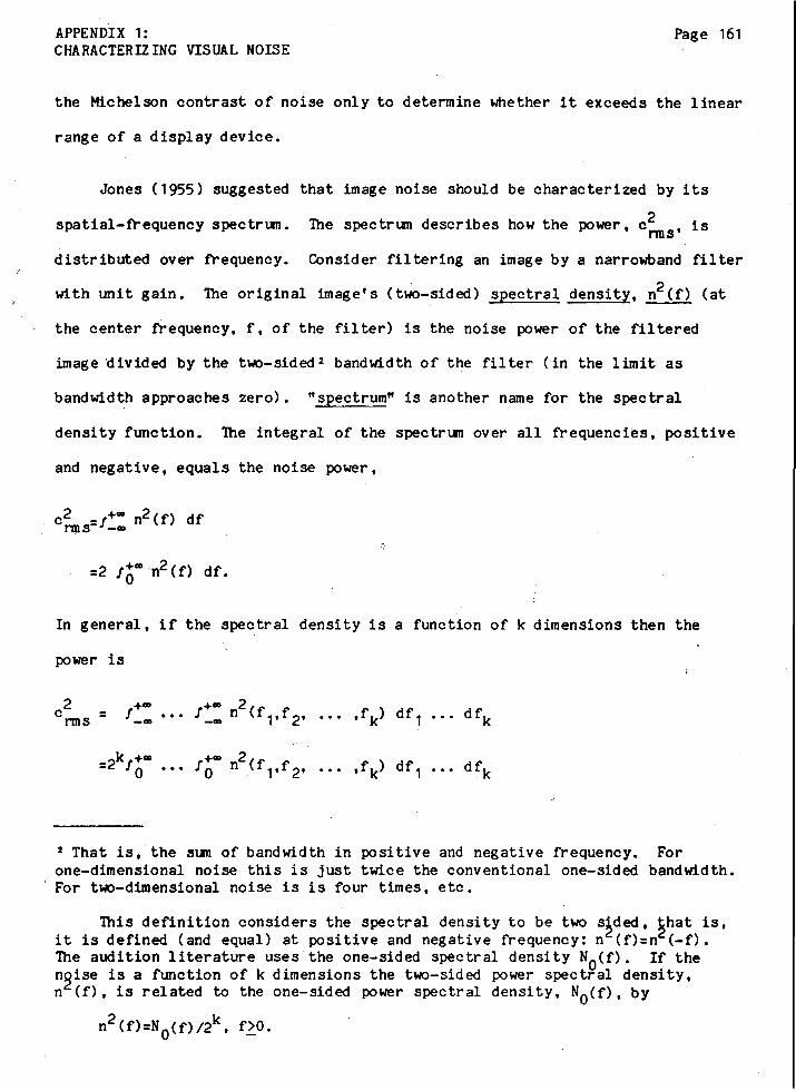
APPENDIX 1: Page 161 CHARACTERIZING VISUAL NOISE
the Michelson contrast of noise only to determine whether it exceeds the linear
range of a display device.
Jones ( 1955} suggested that image noise should be characterized by its
spatial-frequency spectrum. The spectrum describes how the power, c2 , is nns
distributed over frequency. Consider filtering an image by a narrowband filter
with unit gain. The original image's (t~-~ided) spectral density, n2 (f} (at
the center frequency, f, of the filter) is the noise power of the filtered
image 'divided by the two-sided 2 bandwidth of the filter (in the limit as
bandwidth approaches zero). "spectrum" is another name for the spectral
density function. The integral of the spectrum over all frequencies, positive
and negative, equals the noise power,
In general, if the spectral density is a function of k dimensions then the
power is
= +• 2 I -• n ( f 1, f 2 ,
2 That is, the sum of bandwidth in positive and negative frequency. For one-dimensional noise this is just twice the conventional one-sided bandwidth. For t~-dimensional noise is is four times, etc.
This definition considers the spectral density to be two s~ded, ~hat is, it is defined (and equal) at positive and negative frequency: n (f)=n (-f). The audition literature uses'the one-sided spectral density N0(f). If the n~ise is a function of k dimensions the two-sided power spectral density, n (f), is related to the one-sided power spectral density, N0(f), by
n2 Cf}=N 0(f)/2k, f>O.
Page 1o2 CHARACTERIZING VISUAL NOISE
2 To summarize, the square of the rms contrast crms is the power crms•
n2 (f) is the power spectral density of the image at each frequency. The
integral of the spectral density, n2 (f), over all frequencies equals the power,
c2 rms·
In practice most convenient sources of noise produce "white" noise. Noise
is white if its spectral density is constant at all frequencies
( · n2 (f) 1.e. = n2 ). 3 White noise can never be realized in practice because it
would require infinite power. This is not a problem because white noise is
used as an input to systems of limited bandwidth; it is sufficient to make the
spectral density constant from zero frequency through the highest frequency to ---.]
which the observer is sensitive. Thus low-pass white noise will often be
called simply "white".
Now consider measurement. Beginning in 1920 photographic scientists
devised one measure afte'r another of image noise, striving to find the best
correlate of apparent graininess of photographic film. · The diversification
ended when Marriage and Pitts (1956) showed that all the popular measures,
including the spectrum, were equivalent in the sense that any one could be
calculated from any other.
The easiest and oldest objective measure of luminous fluctuation is the
variance of the normalized readings by a photometer which scans the image with
a sampling aperture ("normalized", as before, means divided by the overall
average). For a grainy photograph a small disk is an appropriate sampling
aperture. In general one must specify the sampling aperture extent in each
dimension of variation of the noise. Thus, for a grainy movie one would
' White Gaussian noise has the additional characteristic that the phases of all frequencies are inti epend ent.
APPENDIX 1: • Page 163 CHARACTERIZING VISUAL NOISE
specify the height, width and duration of the sampling aperture. The "aperture
size" is the generalized volune of the aperture. For dynamic t\«>-dimensional
noise the size of an appropriate aperture \«>Uld be height x width x duration;
for static one-dimensional noise the aperture size would be its width.
Each luninance sample will be the average luninance in the sampling
aperture, so the measured luninance function will be "smoother" than the actual
luminance function. As a result the measured power may be less than the actual
2 power, crms· As a result the power of the measured luminance function may be
less than the power of the actual luminance function. If the aperture
dimensions are small relative to one half period of every frequency contained
in the noise, then the measured power will equal the actual power, c~s.
Selwyn (1935) showed that if th~ fluctuations are uncorrelated from point
to point then the product of the aperture area and the measured variance (of
the contrast function~ readings) is constant. Let us call this the
aperture-power product. If there are short-range correlations, for example due
to the finite size of the silver grains, th~n the constancy will hold only .for
apertures substantially larger than the range of the correlations. When the
aperture-power product is specified as a constant it is implied that all large
apertures used for measuring it \«>Uld give the same value.
It would be historically appropriate to call the square root of the
aperture-power product "granularity". Marriage and Pitts ( 1956) said,
"If a piece of photographic material is uniformly exposed and processed and then examined closely it _is seen to be nonuniform in transmission. The visual appearance of irregularity is called graininess; physical measurements of the fluctuation in transmission factor or in optical density are generally called measurements of granularity • • • [Selwin ( 1935)] proposed that granularity be measured by ala [where !!_ is the
~To be precise, Selwin refered to density (i.e. minus logarithm of transmission) readings from a microdensi tometer, not luminance readings from a photometer, but the argument is the same.

n••~UV~A lo • Page lb"
CHARACTERIZING VISUAL NOISE
standard deviation of the normalized density readings, and a is the area of the sampling aperture]. we shall call the curve of ala as a function of a the Selwyn granularity curve, or simply the granularity, its variation with~ being understood."
Defining granularity as the square-root of the aperture-power product differs
from Marriage and Pitts only in being generalized to other than two dimensions,
and in being based on luminance readings, rather than density or transmission
readings.
White noise satisfies Selwyn's requirement that fluctuations be
uncorrelated from point to point (as long as the aperture is large relative to
one half period of the highest frequency in the noise). Jones (1955) showed
that if the noise is white then the aperture-power product does not depend on
the aperture size (within the above constraint) and is equal to the power
spectral density, n2 , of the noise 5 , and, conversely, if the aperture-power
product does not depend on the aperture size then the noise is white. Of
course, the same arguement applies to their square roots: a constant
granularity is equivalent and equal to a constant n, the square root of the
spectral density. The aperture-power product (or its square root, the
granularity) is the easiest way to measure the spectral density of white noise.
In summary, sampling apertures much smaller than half a period of the
highest noise frequency will give a constant power equal to the noise p6wer
c~s; if the noise is white then apertures much larger than half a period of
the cut-off frequency will give a constant aperture-power product equal to the
spectral density, n2 .
One more description of noise should be mentioned. Several important
studies used ideal image intensifiers which displayed a small brief dot (or
"speck") of light for each detected photon (e.g. Rose 1948, van Meeteren and
l
l I [
r
I r
f
[
t
1.
I r

APPENDIX 1: Page 165 CHARACTERIZING VISUAL NOISE
Boogaard 1973). Since the dots are statistically independent the noise is
white and may be characterized by an aperture-power product, as discussed
above. The aperture-power ·product, and thus the spectral density, of dot noise
are equal to the inverse of the dot flux.
Power or spectral density?
Power and spectral density are complementary measures. In the ideal,
white noise has a constant spectral density and infinite power. It is fully
ch~racterized by its spectral density. <At the other hand, the limit of the
narrow-band case, a sinusoidal grating, has infinite power spectral density but
5 Here follows a simple proof that the aperture-power product of wh~ te noise equals its ~wer spectral density. Suppose the spectral density, n (f), is a constant, n , up to a cut-off frequency fc and zero beyond it. The integral for total noise power is
=
2 = 2 fc n •
The noise, having cut-off frequency f , may be fully represented by samples spaced at intervals of 1/(2fc). Furtfiennore those samples will b2 uncorrelated. The sample variance is equal to the noise ~wer, cnns· The a~erage of J uncorrelated variables, each with variance crm , has variance c /J. Thus the
2variance measured with a large aperture ~ich includes J
s~Bles will be c /J. The aperture-power product is the product of aperture size and measured~~riance:
. - n2 - 0
This completes the proof. Note that this also shows that the aperture-power product is the same for all aperture sizes that are large relative to 1 /( 2f ) , c a half period of the cut-off frequency, fc.

APPENDIX 1: Page 166 . CHARACTERIZING VISUAL NOISE
finite power ( c~s equals half the square of the Michelson contrast of a
sinusoid). In practice we will often need to describe band limited white noise.
If the bandwidth exceeds the bandwidth of-the optics of the eye it is clear
that further increases in bandwidth can have no effect on the retinal image.
The noise power, c~s• is of little consequence in this situation. Spectral
density is all we would need to know. In the review of critical-band
experiments it will emer.ge that the relevant visual bandwidth that divides
broad from narrow is the one-to-two-octave bandwidth of a spatial-frequency
channel, rather than the much broader bandwidth of the optics of the eye used ~
in the argument above.
The effect of viewing distance
Since we are primarily interested in the pattern produced on the
observer's retina, the lengths which appear implicitly in the above definitions
(e.g. aperture size, spatial frequency, dot flux) should be measured as angles
sub tended at the observer's eye. Stepping away from a periodic wallpaper
. pattern increases its spatial frequency from the point of view of the observer,
but its rms contrast and its Michelson contrast are dimensionless and
independent of viewing distance. So much is obvious. Not so familiar is the
dependence of contrast spectral density upon viewing distance. Consider
two-dimensional static noise with specltrum n2 ( f x ,f y> or or two-dimensional
dynamic noise with spectrum n2 ( fx ,f Y ,f t) . Doubling the viewing distance
doubles the spatial frequencies in both horizontal and vertical dimensions.
Recall that the spectral density is the power per unit (two-sided) bandwidth.
The power, c~s• is unchanged, but the spatial bandwidths are doubled. It
follows that doubling the viewing distance quarters the spectral density. The
new spectrum is

APPENDIX 1: Page 167 CHARACTERIZING VISUAL NOISE
or
The same power has been distributed over a larger bandwidth.
This may be most easily seen by considering dot noise. We saw earlier
that the spectral density of dot noise is equal to the inverse of the dot flux,
and doubling the viewing distance obviously quadruples the dot flux.
For one-dimensional noise there is only one spatial bandwidth to be
doubled, and so the spectral density is only halved: if the initial spectrun
were n2 <fx), then doubling the viewing distance would make it
n' 2 (fx) = ~ n2 (fx/2).
The effect of viewing distance may have been the first psychophysical
measure of visual noise. Jones and Higgins ( 1945) say,
"Some of the earliest work done on the study of the graininess of photographic deposits was reported in publications from these [Kodak Research] Laboratories (Jones and Deisch 1920, Hardy and Jones 1922). A method was used in which an enlarged image of the uniformly exposed and developed photographic material was moved away from the observer until it appeared homogeneous. the relative merging distances for different samples were used to evaluate graininess. It was found possible to make measurements with a precision which gave an average deviation of ±3 percent. A similar method was used by Crabtree to compare the graininess of motion-picture films."
If the film noises were white over the bandwidth of the observer's visual
optics, then, the effect of increasing the viewing distance was simply to reduce
the power spectral density to threshold.
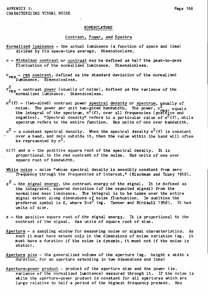
APPENDIX 1: Page 168 CHARACTERIZING VISUAL NOISE
NOMENCLATURE
Contrast, Power, and Spectra
Normalized luminance - the actual luminance (a function of space and time) divided by its space-time average. Dimensionless.
c - Michelson contrast or contrast may be defined as half the peak-to-peak fluctuation of the normalized luminance. Dimensionless.
crms - ~ contrast, defined as the standard deviation of the normalized luminance. Dimensionless.
c~s - contrast power (usually of noise), defined as the variance of the normalized luminance. Dimensionless.
n2 (f) - (two-sided) contrast power spectral density or spectrum, usually of noise. The power per unit two-~ided bandwidth. The power, c2 , equals the integral of the spectrum, n (f), over all frequencies (po~€~ve and negative). "Spectral density" refers to a particular value of n (f), while spectrum refers to the entire function. Has units of one over bandwidth.
n2 - a constant spectral density. When the spectral density n2 (f) is constant over a band, and zero outside it, then the value within the band will often be represented by n2.
n( f) and n - the positive square root of the spectral density. It is proportional, to the _rms .contrast of the noise. Has units of one over square root of bandwidth.
White noise - noise "whose spectral density is sensibly constant from zero --frequency through the frequencies of interest," (Blackman and Tukey 1958).
s 2 - the signal energy, the contrast energy of the signal. It is defined as the integrated, squared deviation (of the expected signal) from the normalized mean luminance. The integral is to be taken over the entire signal extent along dimensions o~ noise fluctuation. In audition the preferred symbolisE, where E=s (eg. Tanner and Birdsall 1958). It has units of size •
. s - the positive square root of the signal energy. It is proportional to the contrast of the signal. Has units of square root of size.
Aperture - a sampling windo~ for measuring noise or signal characteristics. As such it must have extent only in the dimensions of noise variation (eg. it must have a duration if the noise is dynamic, it must not if the noise is static).
Aperture size- the generalized volume of the aperture (eg. height x width x duration, for an aperture ex tending in two dimensions and time)
Aperture-power product - product of the aperture size and the power ( ie. variance of the normalized luminance) measured through it. If the noise is white the aperture-power product is constant for all apertures which are large relative to half a period of the highest frequency present. Has

APPENDIX 1: Page 169 CHARACTERIZING VISUAL NOISE
units of size.
Granularity - the positive square root of the aperture-power product. Originally defined by Selwyn (1935) in a slightly different way.
Dot rate - the average number of statistically-independent, identical spots of ---light per unit aperture. Its inverse is the spectral density of the dot
noise. Has units of one over size.
Critical Spectral Density - The spectral density of a noise mask which raises the squared threshold to twice its zero-noise value. All relevant studies have reported that the square of the contrast threshold is proportional to the sum of the actual and critical spectral densities of noise masks. Has the same units as spectral density.
Transduction Efficiency- the ratio of the photon noise, n~hotons to the observer's equivalent noise, measured in practice as n critical:
TE - (n2 I 2 ) - photons "critical •
Signal detection theory
s/n - signal-to-noise ratio. The terms s and and n were defined above. When a signal is added to white Gausian noise whose bandwidth includes the entire signal bandwidth then the detectability of the signal by an ideal observer which kno·ws .the .. signal exactly is ·'determined only by this ratio. Most of the communication theory and audition literatu~e represents this as 1(2E/N0), where E is the signal energ2 (ie. s ), and N0 is the one-sided spectral density of the noise ( ie. n =N 0;2, assuming tne noise is a function of time only, as is usually the case in audition). If the ~oise were a function of k dimensions the two-sided spectral density would be N0;2k, and the signal-to-noise ratio would be 1(2kE/N o>. Barlow ( 1978) represented the signal-to-noise ratio by d]: (ie. df:s/n). Dimensionless.
d' - the signal-to-noise ratio (defined above) that an ideal observer would require to match a given performance by an observer under study (Tanner and Birdsall 1958). For 2-al ternative forced-choice responses, if the signal is known exactly, d' equals 12 times the normal deviate corresponding to the proportion correct, P(C) (Green and Swets 1966). Dimensionless.
Efficiency - the ratio ( d' >2 /( s/n) 2 (Tanner and Birdsall 1958). Also called "detective efficiency". Dimensionless.
Quantum Efficiency - the special case of efficiency when there is no ltrninance noise. Often defined as the fraction of the corneal quanta which an ideal would have required to perform as well as the observer under study (Barlow 1958b, Jones 1959, Barlow 1962a ,b). Dimensionless.

APPENDIX 2: Page 170 CROSS-CORRELATION AND ENERGY DETECTORS
APPENDIX 2
CROSS-CORRELATION AND ENERGY DETECTORS
Evidence for independent detection of spatial frequencies differing by
more than an octave makes it reasonable to suppose that the eye, like the ear,
may be considered a bank of parallel detectors, each sensitive to only a band
of frequencies. But what sort of detector?.
Two models will be considered. Firstly, coherent detection: a
cross-correlation detector integrates the product of the input and the expected
signal. This is ideal when the signal is known exactly. Secondly, incoherent
detection: an energy detector integrates the square of the filtered input over
the known signal extent and duration. Without the input filter the energy
detector provides ideal detection of a noise increment, thus it represents an
extreme in its high signal uncertainty (Green and Swets 1966).
The operation of cross-correlation is equivalent to convolution by the
time-revers~d expected-signal, and evaluating the result at the origin. Thus
both detectors may be characterized as having an input filter with a modulation
transfer function jH(f) I· Only the relative gain matters so arbitrarily take
jH(f)l to be unity at its peak.
The signal-to-noise ratio at the outputs of the cross-correlation and
energy detectors will now be derived.
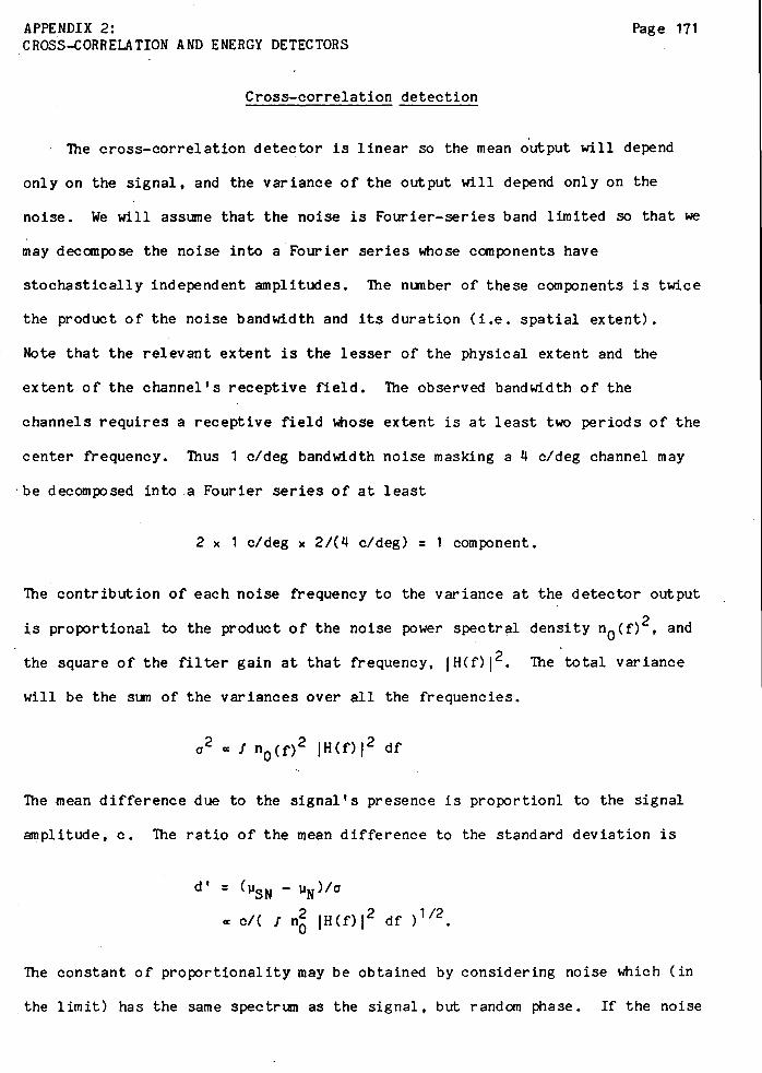
APPENDIX 2: Page 171 CROSS-CORRELATION AND ENERGY DETECTORS
Cross-correlation detection
The cross-correlation detector is linear so the mean output will depend
only on the signal, and the variance of the output will depend only on the
noise. We will assume that the noise is Fourier-series band limited so that we
may decompose the noise into a Fourier series whose components have
stochastically independent amplitudes. The number of these components is twice
the product of the noise bandwidth and its duration (i.e. spatial extent).
Note that the relevant extent is the lesser of the physical extent and the
extent of the channel's receptive field. The observed bandwidth of the
channels requires a receptive field fthose extent is at least two periods of the
center frequency. Thus 1 c/deg bandwidth noise masking a 4 c/deg channel may
be decomposed into a Fourier series of at least
2 x 1 c/deg x 2/(4 c/deg) = 1 component.
The contribution of each noise frequency to the variance at the detector output
is proportional to the product of the noise power spectral density n0 (f) 2 , and
the square of the filter gain at that frequency, IH(f)l 2 • The total variance
will be the sum of the variances over all the frequencies.
The -mean difference due to the signal's presence is proportion! to the signal
amplitude, c. The ratio of the mean difference to the standard deviation is
d' = (pSN- pN)/a
« c/( 1 n~ IHCf>l 2 df >112 •
The constant of proportionality may be obtained by considering noise which (in
the limit) has the same spectrlll'l as the signal, but random phase. If the noise

APPENDIX 2: Page 172 CROSS-CORRELATION AND ENERGY DETECTORS
and signal spectra are equal, the phase specificity of the cross-correlation
detector will give a d' of 12. Thus
d' = 12 c/( J n~ jH(f)j 2 df ) 112.
Energy detection
In audition there is some evidence that detection is effectively mediated
by energy detectors at the output of each filter. Until recently it was
erroneously asstllled that the performance of an energy detector would depend
only on the ratios of signal to noise energies which it received. However
Green and Swets ( 1966) and Patterson and Henning ( 1977) have pointed out that
the performance of an energy detector is determined by the ratio of signal
energy to the standard deviation of the noise energy.
The energy detector is nonlinear and therefore more difficult to analyze
than the cross-correlation ~etector. The mean difference in energy output is
approximately' the energy of the signal ( 1/2 )c2T (where T is the known signal
duration). The variance of the output energy is a sum of contributions from
all the Fourier components of the noise; the variance of each component is
proportional to the product of n6(f) an.d jH(f) 14 • So
' Patterson and Henning (1977) found that the nonlinear interaction of the signal and noise results in a noncentral Chi-square distribution at the detector output. However if the ratio of the signal power times duration to the noise power spectral density is greater than 3 (and the auditory thresholds they report all have ratios in excess of 10) then ignoring the signal-dependent component of the variance leads to underestimating the filter gain jH(f) 1 by less than 5%.

APPENDIX 2: Page 173 CROSS-CORRELATION AND ENERGY DETECTORS
Solving the d_erived equations for the contrast at threshold shows that
they have a very similar form.
c = 12 d' (In~ !H(f)l 2 df >112 (cross-correlation detector)
c = k /(d'T) ( 1 nci 1H(f)l 4 df >114 (energy detector)
G: what is meant by threshold criterion? Isn't T just he signal duration, and
thus known to be constant? It seems reasonable to suppose that d' and Tare ,
constant for a fixed threshold criterion (i.e. 82~ correct), so that relative
threshold elevation will not depend on these unknown parameters. Letc · all-pass
represent the threshold contrast in all-pass white noise whose noise spectral
2 density is "all-pass· Normalizing by the all-pass threshold gives
c -----= c all-pass
IH(f)I2B df}1/(2B)
{ I 2B IH(f)I2B df}1/(2B) "all-pass
where 1/(2B) is the index of summation: 1/2 for the cross-correlation detector,
and 1 /4 for the energy detector.
We may try to understand this last equation. If the output of a detector
increases as the B-th power of its input then its output variance will
increase, approximately, as the 2B-th power of the amplitude of any input
noise. Neglecting distortion products, the frequency components of the noise
are independent so the total output variance will be a sum of the variances due
to each of the components of the noise. The output amplitude of the signal is
the B-th pwer of the input amplitude, so the signal amplitude required for a
given d' will be proportional to -the 1/B power of the output standard
deviation, or the 1/(2B) power of the output variance.

APPENDIX 2: Page 174 CROSS-CORRELATION AND ENERGY DETECTORS
The two detectors differ in several respects. We have seen that threshold
is proportional to an integral over noise frequencies with exponent 2B. In the
cross-correlation detector d' is proportional to the signal amplitude c. In
the energy detector d' is proportional to the signal power c2• In both cases
~· is proportional to c8 . What is the experimental finding? For 2IFC d' is
equal to 12 times the normal deviate corresponding to the proportion correct.
For detection of gratings, Nachmias and Sansbury ( 1974) found that d' increased
2 2 . 2 9 as c • for one observer, and c • for another, and Foley and Legge ( 1981 )
·:r..-... ·-_
report exponents between 2.11 and 3.04 for two observers at three different
spatial frequencies (.5, 2, and 8 c/deg). Neither the cross-correlation nor
the energy detector has a psychometric function as steep as these. The above
derivations are general enough to allow for B to be say, 3. Alternatively,
channel uncertainty among a large number of cross-correlation detectors (or
energy detectors for that matter) would generate psychometric functions of the
required steepness, but that is the topic of Chapter 5.

APPENDIX 3: Page 175 THE EFFECTS OF HETERODYNE NOISE
APPENDIX 1
THE EFFECTS OF HETERODYNE NOISE ------- -- -----
Heterodyne means that the two sidebands are symmetric about the carrier
frequency, i.e. the components at frequencies~-~ and~+~ have even-symmetric c c
amplitude and odd-symmetric phases 7 • The most obvious manifestation of this
symmetry is that the heterodyne noise has zero crossings at all the zero
crossings of the original carrier (Spiegel 1979).
Correlation between the sidebands complicates the analysis of the total
variance produced in a channel because it is normally assumed that each
frequency component of the noise makes an independent contribution to the
variance in the channel. Nevertheless this has been the technique most often
used in audition to produce narrowband noise (e.g. Greenwood 1961).
In audition the channels are thought to be non-phase-specific energy
detectors, so the phase symmetry is not a concern. However the amplitude
symmetry would cause a channel symmetric about the carrier frequency to receive
equal contributions from each sideband, so the standard deviations would add,
instead of the variances, as would happen if the components were independent.
In vision the spatial-frequency channels may be phase specific. I will
now calculate the response of a cross-correlation detector to a symmetric pair
of components of heterodyne noise. The input is
The output will depend only on the amplitude and phase of ~he expected signal
7 Phases are taken relative to an arbitrary origin at which the cosine carrier is one.

APPENDIX 3: Page 176 THE EFFECTS OF HETERODYNE NOISE
at those frequencies. Let us represent the relevant components of the expected
signal as
~ere S and S' are taken as positive. We want to lmow how the amplitudes s and
S' and the phases e and e' affect the output. The cross-correlation will be
a/2{S cos(e++) + S'cos(e'-+)}
=a/2{[s cos(e)+S 'cos( a' )]cos(+) - [S sin(e)-S 'sin( a' )]sin(+)}
Remembering that a and + are random variables, we 'can see that the output will
be identically zero only if
[S cos(e)+s'cos(e')]=O
and
[ s sin < e ) -s ' sfn ( e ' ) ] =0 •
Alternatively the total will be twice that due to either sideband when
s cos(e)=S'cos(e')
and
s sin(e)=-s'sin(e').
Both alternatives require that
S=S '·
Thus these extremes can occur only when the spectrum of the expected signal is
symmetric about the center of the heterodyne noise. The output will be zero if

APPENDIX 3: Page 177 THE EFFECTS OF HETERODYNE NOISE
6+6 '=11''
and the double-sideband (i.e. total) output will be double the single-sideband
output if
e=-e '.
That is, the response of a cross-correlation detector to heterodyne noise will
differ most from its response to truely-white narrow-band noise of the same
spectrun if
1. the spectrun of the expected signal is symmetric about the carrier
frequency of the heterodyne noise, and either
2a. the phases of the expected signal are odd-symmetric about the carrier
frequency, in which case the output will be twice that due to just one
sideband, or
2b. the phases at frequencies symmetric about the carrier are complementary
angles, in which case the output will be identically zero.
On the positive side it should be noted. that if the spectrun of the
expected signal is very asymmetric with respect to the carrier frequency, so
that the two sidebands of the noise receive very different attenuations, then
the contribution from one sideband or the other will dominate and the symmetry
of the heterodyne noise will not matter. In practice this will mean that the
symmetry of heterodyne noise may safely be ignored, except when the noise is
centered on the channel peak, where channel sensitivity may be overestimated by
as much as 12, or, for phase-specific detection, may be grossly underestimated;
depending on the phase relations of the expected signal and the carrier of the
heterodyne noise.

~rrcnu~A ~;
THE EFFECTS OF HETERODYNE NOISE
Conclusion
The symmetry of heterodyne noise may lead to overestimating the peak
sensitivity of an energy detector by as much as 22, but will not cause an
underestimate. For a cross-correlation detector the peak sensitivity may be
overestimated by as much as 12, or may be grossly underestimated.

APPENDIX 4: Page 179 GENERATING NARROW-BAND NOISE
~APPENDIX 4
GENERATING NARROW-BAND NOISE
The obvious way to produce narrow-band noise would be to pass white noise
through a bandpass filter. However, for ease of analysis it is desireable to
have very steep fall off at the edges of the band. It is diffi.cul t to build an
adjustable bandpass filter with skirts as steep as desired. For conventional
filter designs the steepness of the fall off is inversely proportional to the
cut-off frequency. Three techniques will described which achieve a steep fall
off, independent of cut-off frequency, by doing the filtering at a low
frequency, and then shifting the noise band up to the desired center frequency.
The first technique is simpler but produces heterodyne noise whose frequency
components are not completely independent. The third technique is just an
unconventional-bandpass filter. All these techniques are known, but never seem
to have been collected in one place before.
Analysis of the techniques is facilitated by considering their action on
an arbitrary frequency component of the noise. Over any interval of finite
duration T we may represent white noise by a Fourier series whose components
have stochastically independent amplitudes. Let w be a multiple of 1/T. At
this frequency we have
u cos(wt) + u'sin(wt)
where u and u' are stochastically independent, zero-mean, and Gaussian, and
have equal variance. We may change coordinates to
+=-arc tan ( u' /u) ,

APPENDIX 4: Page 180 GENERATING NARROW-BAND NOISE
so
u cos(wt) + u'sin(wt) = a cos(wt+.).
The new random variables a and • are stochastically independent, • has a
uniform distribution, and a has a Rayleigh distribution.
AM
Greenwood ( 1961) described the simplest technique: (suppressed-carrier)
amplitude modulation (AM), which produces heterodyne noise. A low-pass filter
is used to select a narrow band of noise centered at zero frequency, then this
is multiplied by a carrier, e.g. cos(w0t), of the desired center frequency, w
0•
Consider the effect of this operation on an arbitrary frequency component of
the noise with frequency w, amplitude a, and phase •:
The output will be•
cos(w0 t) a cos(wt+•)=o/2 {(cos(w0t-wt-•) + cos(w0t~wt+.)}
if lwl<w0 , and zero otherwise.
The single input frequency produced two output frequencies with equal
amplitudes and inverted phases (i.e. -• and •). Because each frequency
component of the input produces two symmetric frequency components in the
output the resulting heterodyne noise has twice the bandwidth of the low-pass
• Most of the algebra in this appendix is just repeated application of three trigonometric identities:
cos(a)cos(b):1/2 { cos(a+b) + cos(a-b)} sin ( a) cos ( b) = 1 /2 { sin ( a+ b) + sin ( a-b) } sin(a)sin(b)=1/2 {-cos(a+b) + cos(a-b)}

APPENDIX 4: Page 181 GENERATING NARROW-BAND NOISE
filter.
Unfortunately the effects of heterodyne noise can be considerably more
difficult to analyze than truely white noise (see "The effects of heterodyne
noise"), more than compensating for the relative ease with which it may be
generated. The following techniques produce truely-white narrow-band noise.
Quadrature AM
Spiegel ( 1979) described a technique which may be called quadrature AM
produces a narrow band of noise with no symmetry. Take two independent noise
sources. Pass both through identical low-pass filters. Multiply one by a sine
carrier, multiply the other by a cosine carrier, and then add them 9 • We start
with
a cos(wt++)
and
a' cos(wt++ ')
where a, a', +• and+' are all-stochastically independent. The phases have a
uniform distribution, and the amplitudes have a Rayleigh distribution.
Multiplying by the carriers and adding gives us
a cos(wt++)cos(wct) + a'cos(wt++')sin(wct)
=a/2{cos(wct-wt-+)+cos(~ct+wt++)} + a'/2{sin(wct-wt-+')+sin(wct+wt++')}.
' On a raster-type display this may be achieved by using one noise source and using the sine and cosine carriers on alternate frames of the display, relying on the observer's eye to Sl.ln them.

APPENDIX ~: Page 182 GENERATING NARROW-BAND NOISE
Substituting +"=+ '+tr/2 gives
Define four new random variables,
x=a cos(+)
Y=a sin(+)
x ' = a ' cos ( + ")
y' = a ' sin ( + ") •
These are all stochastically independent, zero mean, and Gaussian. In terms of
these new variables we have
=1/2{(x+x')cos(wct-wt)+(y+y')sin(w t-wt)+(x-x')cos(w t+wt)+(-y+y')sin(w t-wt)}. c c ·~ c
The amplitudes, (x+x'), (x-x'), (y+y'), and (-y+y'), are stochastically
independent, zero mean, and Gaussian. That completes the analysis.
This method requires two independent noise sources, two filters, two
carriers in quadrature phase, and two multipliers. Fortunately some situations
allow multiplexing one noise source, filter, and multiplier between the two
carriers. When that is not possible the following technique may be preferable
as it requires only one noise source, at the expense of using more multipliers.
General purpose band-pass filter
It is possible to use heterodyne techniques to make a steep fall-off
bandpass filter. I do not know who first devised the following technique; for
a discussion of methods of single-sideband modulation see Panter ( 1965). In
order to avoid introducing symmetries the circuit has two pathways, one uses a
I r r I r ["
I I r
l I
APPEND'rX 4: Page 183 GENERATING NARROW-BAND NOISE
sine carrier, the other uses a cosine carrier. In each pathway the input
spectrum is shifted down, low-pass filtered, and shifted back up •. The output
is the sun of the output·s of the two pathways. All shifts are performed by
multiplying by the carrier frequency which also is the center frequency of the
~esulting passband. Again the resulting passband has twice the bandwidth of
the low-pass filter. The circuit is linear so it is sufficient to determine
its output for an input of arbitrary frequency and Jbase:
( 1} cos(wt+p}, where w>O.
First we. multiply by the cosine and sine carriers:
(2}
(2 ')•
Let the cut-off frequency of the low pass filter be w0 , where O<w0 <wc• Then
after filtering we have
(3}
and
(3'}
1/2 cos(w t-wt-+} c
Multiplying by the cosine and sine carriers again gives
( 4}
and
(4'}
otherwise.

APPENDIX 4: Page 184 GENERATING NARROW-BAND NOISE
Finally, the sum of (4) and (4') is
(5) 1/2 cos(wt++) for lwc-wl<w0 , and zero otherwise.
Comparing the ,output, (5), with the input, (1 ), shows that the circuit just
l)alves the amplitude of frequencies inside the passband and stops frequencies
outside the passband. No symmebries are introduced' and the steepness of
cut-off is independent of the center frequency of the pass band.
Summary
Heterodyne noise is easy to produce, but at least in theory, the symmetry
of its sidebands can affect its effectiveness as a mask. Two techniques have
been described which produce truely-white narrow-band noise. Both techniques
require two carriers in quadrature phase. The best choice of method will
depend on the purpose of the experiment and the nature of the dimension along
which the noise varies.

APPENDIX 5: Page 185 OFF -FRECUENCY LOOKING
APPENDIX 5
OFF-FREQUENCY LOOKING
FITTING THE CURVES
The fits used a "flat-top power function", but the following argliDent will
be easier to understand if we first consider a "flat-top exponential".
Consider a channel with a flat top of width fh-fl, and negative exponential
skirts, e-alf-fll and e-bl f-fhl• Let us call this a flat-top exponential.
Note that the skirts would be straight on a graph of log gain versus linear
frequency. !here are four free paraneters; a and b determine the steepness of
the skirts and f1 and fh determine the edges of the nat top. !his shape may
only crudely approximate the actual channel sensitivity, but most of the
measureable properties of a bandpass filter depend only on the width of its
passband and the steepness of its skirts. Since the width of the flat top,
f h-f1 , is free to vary, this model includes a peaked exponential as a special
case.
By asstJDption, for each noise mask, threshold is determined by the channel
with the best s/n. To find this channel Patterson and Nimmo-Smith used an
iterative technique. For each set of channel shape parameters they found the
position of maximum s/n, and compared the predicted threshold with their data.
By iteration they found the most likely channel shape. My model allows a
shortcut.
Suppose a nat-top exponential filter is placed so that both a sinusoidal
signal and a band of noise are passed by one skirt, e-alf-fll. Suppose the
signal frequency fs is greater than f1 , and consider shifting. the filter
towards the signal a small amount Af. Before the shift the signal gain was
e-a(fs-fl). After the shift the signal gain would be e-a(fs-fl-Af). The net

APPENDIX 5: Page 186 OFF -FREQJENCY LOOKING
amplification caused by the shift would be ea ~f. Similarly the filter gain
over the whole noise band would be amplified by ea ~f The signal-to-noise
ratio would be unchanged. Pushing the filter towards the signal increases the
gain for the signal and noise in direct proportion, until the nat top reachs
the signal or noise.
Suppose the top reaches the signal first. Pushing further would anplify
the noise, but not the signal. The s/n at this position is equal or better
than the s/n at all other positions.
Suppose the top reaches the noise first. Pushing further amplifies the
signal and noise but the noise is amplified in less than direct porportion,
until the top reaches the signal. What position maximizes the signal-to-noise
ratio? If the si&nal is outside the noise band, the top of the filter should be
placed on the opposite side of the signal as the noise. If the noise is low
pass, or high pass, so that only one edge of the noise band need be considered,
the top of the filter should be placed on the opposite side of the signal as
the center of the noise band. Finally, if the signal is inside a finite band
of noise then t~1e optimal placement depends on the relative steepnesses of the
two filter skirts.
Host of my data were collected w1 th low-pass or high-pass noise, or narrow
bands of noise which did not include the signal frequency. Assuming the
nat-top exponential shape, the thresholds were determined by only two
channels: one with its top just below the signal frequency when the center of
the noise was above, and one with its top just above the signal frequency when
the center of the noise was be1ow. By this interpretation the low pass masking
thresholds are all from the high channel, and the high-pass masking results are
all from the low channel. On the other hand the narrowband.masking results

APPENDIX 5: Page 187
OFF-FREQUENCY LOOKING
directly outline the upper skirt of the lower channel, and the lower skirt of
the upper channel. The narrowband masking results contain no clue as to the
width of the top of the channel.
The analysis so far has used a linear frequency axis, because the noise
had equal power in equal width bands of linear frequency, however existing
evidence that channel width is about an octave or two independent of frequency
suggests that our model shape should be described on a log frequency axis.
Therefore I fit the data with a nat top and power-law skirts, which are
straight when plotted as log gain versus log frequency. A power law is
steepest near the top so the above conclusions still apply: the low-pass
results should all be from one channel, and the high pass results should all be
from another.
APPENDIX 6: Page 188 THE EFFECT OF UNCERTAINTY
APPENDIX 6
THE EFFECT OF UNCERTAINTY:
DETECTING A SIGNAL AT ONE OF TEN-THOUSAND POSSIBLE TIMES AND PLACES 10 ----- -----
Consider detection of a lmown signal at a specified time and place. That
is how most of us measure a threshold: the same signal is presented in trial
after trial. Every opportunity is usually taken to teach the observer exactly
what he is being asked to detect, including where it will appear, and when,
both as a fixed delay after requesting a trial, and by a simultaneous audible
tone. At the end of each trial the observer thinks about what he saw and
responds. This effort to provide exact lmowledge of the signal raises a
question. Does the observer use lmowledge of the signal to ignore irrelevant
sensations which could not have been due to the signal, in order to give more
accurate responses and thus lower his threshold? If the observer lmows the
signal can only occur at a certain time and place can he ignore other times and
places? How helpful is it to lmow the signal exactly? Existing theories of
visual detection give three incompatible answers.
First, probability summation models usually assume individual units called
"detectors" that are never active in the absence of a signal. This assumption
is usuall~ called a "high threshold". The high-threshold assumption implies \
that the observer does not need the exact lmowledge that is usually provided
because the detector units never give false alarms. In other words there are
no irrelevant sensations to ignore.
1 • This paper was presented at the 1981 meeting of the Association for Research in Vision and Ophthalmology, in Orlando, Florida (Pelli, 1981).

APPENDIX 6: Page 189 THE EFFECT OF UNCERTAINTY
At the other extreme the Theory of Signal Detectability has shown that the
ideal way to detect a known signal is to cross-correlate by the signal itself
(Peterson, Birdsall, and Fox 1954). Various discrepancies between such a
cross-correlation model and actual human performance have led to variants such
as incorporating a nonlinear transformation, and supposing that we only have a
fixed set of weighting functions available and that we use the one most similar ·
to the signal. All these models require prior knowledge of the signal in order
to choose the best weighting function. Without prior knowledge of the signal,
simple cross-correlation would be inefficient and performance would suffer
greatly.
Halfway in between these extremes lies the hypothethis of high intrinsic
uncertainty. This too was inspired by developnents in the Theory of Signal
Detectability. In many ways human detection of a known signal' is similar to
.. ideal detection of one of ~any possible signals. According to the uncertainty
hypothesis, the observer has a very limited ability to use prior knowledge,
that is, he is intrinsically uncertain.
Let me recap. According to the high-threshold hypothesis, exact knowledge
of the signal is superfluous. For the cross-correlation hypothesis exact
knowledge of the signal is crucial. According to the uncertainty hypothesis
attempts to provide knowledge of the signal provide only a small benefit to the
observer. To test these predictions I measured the effect of depriving the
observer of exact knowledge of the signal.
The signal was a brief, thin, bright, vertical bar on a large uniform
background with a luminance of 340 cd/m2 • It was { 0 wide and lasted for 20
msecs. (The display was 27° wide and about half as high.) In the center of the
display was a large fixation cross, which the observer was always instructed to

APPENDIX 6: Page 190 THE EFFECT OF UNCERTAINTY
fixate. In all cases the data are the responses from two-interval forced
choice trials with feedback. The thresholds I will report are maximum
likelihood estimates of the contrast required for 82S correct.
The first phase of the experiment measured contrast thresholds at 2°
intervals across the visual field. In order to provide the observer with exact
knowledge of the signal, moveable large arrows above and below the display
indicated exactly where the signal would appear, and each interval of the 2IFC
trial was mar ked by a 20 msec beep which was simultaneous with the 20 msec
signal.
Figure 1: threshold profiles for DP and OK
This slide shows the contrast threshold at each eccentricity for two observers.
Viewing was binocular. The blind spots would be off the graph. Each point is
an independent threshold estimate based on 50 trials. The kinky lines through
the data connect up the means at each eccentricity for each observer. Those
lines were taken as the observer's threshold profile over this part of the
visual field. In the rest of the experiments all contrasts will be relative to
these nominal threshold profiles for each observer.
In the main phase of the experiment, the signal could appear, randomly, at
any of the 97 contiguous locations from -12 to +12 degrees eccentricity, and
each interval of the 2IFC procedure was accompanied by a 2000 msec beep and the
20 msec signal could occur at any time during the beep. Since the signal could
appear at any of 97 places and 100 times, there were 9,700 possible times and
places. The staircase procedure controlled the contrast of the signal relative
to the nominal threshold profile.

a_~
00
I I -00
0 r ~ •
0
0
0 __..o ..--+
~ 0
0 1
0
0
I .--0 •
0
_____.. 0 ....... I
Figure 1
::J) +-~-u -L + c Q) l) ()
LLI
·-:

APPENDIX 6: Page 191 THE EFFECT OF UNCERTAINTY
Figure 2: DP, M=9, 700
!i is the degree of uncertainty introduced experimentally, 9, 700 in this
case. The ordinate on the right is proportion correct. The abscissa is
contrast relative to the nominal threshold profile. The left ordinate is d'
and is labeled ,12z. 11 First consider the X's, on the right. They show the
proportion correct obtained for detection at each contrast.
There are different numbers of trials at each contrast. The vertical bars
are 95% confidence intervals. The solid curve is the maximum likelihood,
two-parameter, fit by a Qlick ( 1974) function. Detection threshold, that is,
the contrast for 82% correct is 1.4.
When I did this experiment it occurred to me that in addition to detection
it would be interesting to also measure contrast discrimination. Lasely and
Cohn ( 1981 ) have pointed out that uncertainty might be expected to have much
less effect on discrimination than on detection. In a contrast discrimination
experiment the stimulus appears in both intervals, but at different contrasts.
The lower contrast is the pedestal contrast and is the same in each trial. The
11 This is d' as defined by Green and Swets ( 1966). As defined by Tanner and Birdsall ( 195 8), d' is the signal-to-noise ratio that would be required by an ideal to perform as well as the observer under study did. Since the signal was experimentally uncertain the ideal would b.e a 9, 700-channel-uncertainty model, whose performance, as measured by 12z, rises as the 3.5 power of contrast:
12z « c3· 5,
as shown in Figure 5. Figure 6 shows that in the uncertainty condition both human and ideal performance rise as the same 3. 5 power of contrast, implying that, as defined by Tanner and Birdsall ( 1958), the obsever' s d' is proportional to contrast:
d' «c.

Observer DP, M= 9700 Figure 2
10
.999
.99
/~/ ~
.90
.80 I .76
+-/ ,' .70
(.) Q.) ~ ,' ~
0 (.)
-{2Z .60 c 0 +-~
0 0. 0
.55 ~
a_
.I .53
.51
nt~----------~~--~--------~ .I 10
Contrast
(relative to nominal threshold}

APPENDIX 6: Page 192 THE EFFECT OF UNCERTAINTY
higher contrast is higher by an amount called the difference contrast.
The O's show discrimination of difference as a function of difference
contrast, relative to the nominal threshold profile. In order to make the
conditions of contrast detection (the X's) and discrimination (the O's) as
co~parable as possible the two conditions were randomly interleaved. The
observers did not know whether a given trial was contrast discrimination or
detection; he was instructed to always choose the interval with higher
contrast.
In contrast discrimination trials the stimulus was presented at the same
randomly determined time and place in both intervals.
These thresholds in uncertainty are based on contrasts relative to the
nominal threshold profile at many eccentricities. Samll inaccuracies in the
nominal threshold profile might be systematically biasing these thresholds. To
control for this possibility I measured a similar threshold for the
no-uncertainty condition.
Figure 3: DP, M:1
The same procedure was used except that the beep for each interval was
reduced from 2000 msec to 20 msec and coincided with the signal, and the
signal, instead of appearing randomly at any place on the display, appeared,
consecutively, at each position on the display. In the first 5 or 6 trials it
appeared at -12° (near the left edge of the display), in the next 5 or 6 trials
it appeared at -11.75° and so on until in the last 5 or 6 trials it appeared at
+12° (near the right edge of the display). Pointers above and below the
display indicated where the signal would occur, and were adjusted every few

-{2Z
Observer DP) M=1 10
.I
Figure 3
.. 999 .99
.90
.80
.76
.70
.60
.55
.53
.51
.01 ___ ..._ ........................... ..__...__..~...~~...L.L.I .I 10
Contrast
(relative to nominal threshold)
+-() Q) ~
~
0 U. c: 0 +-~
0 0.. 0 ~ a..

APPENDIX 6: Page 193 THE EFFECT OF UNCERTAINTY
trials to keep up with the signal. As before the observer fixated the fixation
cross continuously, and all contrasts were relative to the nominal threshold
profile.
These results have the familiar form described by Nachmias and Kocher
(1970): discrimination is better than detection. Detection has a threshold of
.9 and a steep psychometric funcion. Discrimination has a lower threshold, .4,
and its psychometric function has approximately unity slope in these
coordinates.
Before comparing the results with and without uncertainty I would like to
ask for your indulgence to briefly consider what the Theory of Signal
Detectability has to say about effects of uncertainty on ideal performance.
Ideal performance for detection of a known signal is shown on the next slide.
Figure 4: ideal, M=1
As before the ordinate is d'. 12 The abscissa is the signal-to-noise ratio,
which we may assume is proportional to contrast. In these coordinates the
psychometric function has unity slope. The psychometric function is the same
for detection and discrimination.
Figure 5: ideal, M=10,000
The graph on the right shows the ideal performance for detection of one of
10,000 orthogonal signals. 13 Relative to the no-uncertainty case we just saw,
threshold is higher and the function is steeper. On the left is the ideal
12 Again, the ordinate is 12 times the normal deviate corresponding to the proportion correct, which Green and Swets (1966) would call "d'", but not Tanner and Birdsall ( 1958).

Ideal, M= 1
s/n
Figure 4
.999
.99
.90
.80
.76
.70
.60
.55
.53
.51
~
(.) C1) .... .... 0 (.)
c: .Q ~ .... 0 0. 0 .... a..

10
.. -{2 z
.I • • • • •
• • ..• • • •
Ideal_, M= 10,0CX)
• • • • • • • • • • •
• • • • • •
• • •
• • • •
• .. . . . . • . . . • • . . • • • • • •
s/n
• • . . • . •
• • • •
•· • • • • • • • • • • • • • • • . .
• • • • • • • • • • • • • • • • • • • • • • • • • • • • • • • • • • • • • •
Figure 5
.999
.99
.90
.80
.76
.70
.60
.55
.53
.51
~
() Q) ~
~
0 u c 0 ·-~ ~
0 0. 0 ~
Q_

APPENDIX 6: Page 194 THE EFFECT OF UNCERTAINTY
performance for contrast discrimination, assuming the pedestal is highly
detectable on its own. 1 ' The discrimination function has unity slope, just as
without uncertainty. Uncertainty has very little effect on ideal
discrimination performance if the pedestal is highly detectable on its own (see
~.g. Lasely and Cohn 1981).
Figure 6: DP and Ideal
This last slide compares the observer's performance with and without
uncertainty. The solid curves show the observer's psychometric function for
the no-uncerta.inty condition. The dashed curves show his psychometric
functions for 9,700-fold uncertainty. The uncertainty raised threshold by a
.factor of 1.5 for detection and by about 1.2 for discrimination. The small
effect of uncertainty on threshold for detection and the even smaller effect of
uncertainty on disorimination is consistent with the hypothesis of high
intrinsic uncertainty.
The dotted lines are the ideal psychometric functions for 10,000-fold
uncertainty. The constant of proportionality between signal-to-noise ratio and
contrast was arbitrarily adjusted to slide the two ideal psychometric functions
horizontally to the observer's psychometric functions for the no-uncertainty
condition. The observer's psychometric functions without uncertainty are
u Peterson, Birdsall, and Fox (1954), Nolte and Jaarsma (1967), and Pelli ( 1980)
1' The calculation asstll'led that the pedestal contrast had a detectability of d'=1, i.e. 12z=1.

10
.I
• • • • • • • • •
---Observer DP, M=1 ~~gure 6
--------Observer DP, M=9700
•
················ Idea I J M = 1 O,()(X)
• • • • • • • • • •
• • •
• • • • •
.I
• •
• • • • •
• • •
• • . • . • .. · .1., . .,, .,., .,., .. .,.,
~.,
• .J'
Contrast
• . . .
.999
.99
.90
.80 0
.76 ~ ... 0
.70 u c:
.Q +...
.60 0 a.
.55
.53
.51
0 .... Q_
(relative to nominal threshold)

APPENDIX 6: Page 195 THE EFFECT OF UNCERTAINTY
strikingly similar to the ideal psychometric functions for ten-thousand-fold
uncertainty. Similar detection results have been obtained from a second
observer.
Thus, when the signal could appear at any one of nearly ten-thousand times
and places, the observer's threshold was a factor of 1.5 times higher than when
he was informed when and Y'lere the signal would appear. This rejects the
hig~~hreshold hypothesis which predicted no effect of uncertainty, and
discredits the cross-correlation hypothesis which predicted a large effect. . '', .:~ .,
-with or without ~xperimentally introduced uncertainty the human observer
behaves very much like the ideal observer of one of many possible signals. · It
would seem that the observer has a high intrinsic uncertainty for detection of
thin brief bars.
Page 196
REFERENCES
Abramowitz, H., and Stegun, I.A. (1964) Handbook of Mathematical Functions. Ik>ver Publications, NY
Aguilar, H., and Stiles, W.S. (1954) Saturation of the rod mechanism of the retina at high levels of stimulation. Opttca Acta 1:59-65
Atkinson, J., Campbell, F.W., and Francis, H.R. (1976) The magic number 4±0: a new look at visual numerosity judgements. Perception 2:327-334
Barlow, H.B. (1956) Retinal noise and absolute threshold. Optical Society of America 46:634-639
Journal of the ~~~---
Barlow, H.B. (1957) Increment thresholds at low intensities considered as signal/noise discrimination. Journal of Physiology 136:469-488
Barlow, H.B. (1958) Temporal and spatial summation in human vision at different background intensities. Journal of Physiology 141:337-350
Barlow, H.B. (1958b) Intrinsic noise of cones. Visual Problems of Colour National Physical Laboratory Symposium. H.H. Stationery Office, London. pp. 615-630
Barlow, H.B. (1962a) A method of determining the overall quantum efficiency of visual discriminations. Journal of Physiology 160:155-168
Barlow, H.B. (1962b) Measurements of the quantum efficiency of discrimination in human scotopic vision. Journal of Physiology 160:169-188
Barlow, H. B., MacLeod, D.l. A., and van Heeter en, A. ( 1976) Adaptation to gratings: no compensatory advantages found. Vision Research ~:1043-1045
Barlow, H.B. (1977) Retinal and central factors in human vision limited by noise. in Vertebrate Photoreception Barlow, H.B., and Fatt,P., eds., Academic Press, N.Y.
Barlow, H. B. ( 1978) The efficiency of detecting changes of density in random dot patterns. Vision Research ~:637-650
Barlow, H.B., Levick, W.R., and Yoon, H. (1971) Responses to single quanta of light in retinal ganglion cells of the cat. Vision Research l!L Supplement No • .J_: 87-101 ·
Beurle, R.L. (1969) Visual performance and the use of image intensifiers. NATO Symposium~ Image Evaluatibn _1, Leibowitz, H.W., ed ., Pennsylvania State University, pp. 3-27
Blaclanan, R.B., and Tukey, J. (1958) The Measurement of Power Spectra. Ik>ver Publications, Inc., NY
Blackwell, H. R. ( i 946) Contrast thresholds of the hllllan eye. Optical Society of America 36:624-643
Journal of the
REFERENCES
Blackwell, H. R. ( 1963) Neural theories of simple visual discrimination. Journal of the Optical Society of America 53: 129-160
Page 197
Blakemore, c., and Campbell, F.W. (1969) On the existence of neurons in the human visual system selectively sensitive to the orientation and size of retinal images. Journal of Physiology 203:237-260
Blakemore,.C., Muncey, J.P.J., and Ridley, R.M. (1971) Perceptual fading of a ~tabilized cortical image. Nature 233:204-205
Blakemore, C., Muncey, J.P.J., and Ridley, R.M. (1973) Stimulus specificity in the human visual system. Vision Research jl:1915-1931
Burgess, A.E., Humphrey, K., and Wagner, R.F. (1979) Detection of bars and discs in quantum noise. Proceedings of the SPIE 173:34-40. (Bellingham, WA 98225)
Burgess, A.E., and Barlow, H.B. (1981) The precision of judging the number of dots in a random array., submitted to Vision Research
Burgess, A.E., Wagner, R.F., Jennings, R.J., and Barlow, H.B. (1981a) Efficiency of human visual signal discrimination. Science, in press
Burgess, A.E., Wagner, R.F., Jennings, R.J., and Barlow, H.B. (1981b) Absolute efficiency of human visual signal detection and discrimination. submitted to Journal of the Optical Society of America
Campbell, F.W., and Gubisch, R.W. (1966) Optical quality of the human eye. Journal of Physiology 186:558-578
Campbell, F.W., and Green, D.G. (1965) Optical and retinal factors affecting visual resolution. Journal of Physiology 181:576-593
Campbell, F.W., and Robson, J.G. (1968) Application of Fourier analysis to the visibility of gratings. Journal of Physiology 197:551-566
Campbell, F.W., and Kulikowski, J.J. (1966) Orientational selectivity of the human visual system. Journal of Physiology 187:437-445
Carter, B.E., and Henning, G.B. (1971) The detection of gratings in narrow-band visual noise. Journal of Physiology 219:355-365
Chambers, R.P., and Courtney-Pratt, J.S. (1969) Experiments on the detection of visual signals in noise using computer-generated signals. Photographic Science and Engineering 11:286-298
Chesters, M.S. (1973) The Influence of Visual Noise on Visual Detection Thresholds, PhD. thesis:-University of Leeds
Chesters, M.S., and Hay, G.A. (1979a) The influence of visual noise on visual threshold detection. unpublished manuscript
Chesters, M.S., and Hay, G.A. (1979b) The relation between signal area and threshold-limiting noise. unpublished manuscript

REFERENCES Page 198
Cohn, T.E. (1976) Detectability of a luminance increment: effect of superimposed rand an luninance fluctuation. Journal of the Optical Society of America 66:1426-1428
Cohn, T.E. (1981) Absolute threshold: analysis in terms of uncertainty. Journal of the Optical Society of America 1.!: 783-785
Cohn, T.E., Green, D.G.,· and Tanner, W.P.,Jr. (1975) Receiver operating ~haracteristic: application to the study of quantum fluctuation effects in optic nerve of rana pipiens. Journal of General Physiology 66:583-616
Cohn, T.E., and Lasely, D.J. (1974) Detectability of a luninance increment: effect of superimposed randan luninance fluctuation. Journal of the Optical Society of America 66:1426-1428
Coltman, J.W. (1954) Scintillation limitations to resolving power in imaging devices. Journal of the Optical Society of America 44:234-237
Coltman, J.W., and Anderson, A.E. (1960) Noise limitations to resolving power in electronic imaging. Proceedings of the IRE 48:858-865
Dainty, J.C., and Shaw, R. (1974) Image Science, Academic Press, NY
Davenport, W.B. Jr., and Root, W.L. (1958) An Introduction to the Theory of Random Signals and Noise. McGraw-Hill Book--co., N.Y. -- -
Davis, B., and Graham, N. (1979) Uncertainty effects in the detection of sinusoidal gratings. Supplement to Investigative Ophthalmology and Visual Science 18: 244A
Engstrom, R.W. (1974) Quantum efficiency of the eye determined by comparison with a TV camera. Journal of the Optical Society of America Ei= 1706-1710
Fellgett, P.B. (1958) Equivalent quantum-efficiencies of photographic emulsions. Monthly Notices, Royal Astronomical Society 118:224-233
Fletcher, H. (1940) Auditory patterns. Reviews of Modern Physics ~:47-65
Foley, J.M., and Legge, G.E. (1981) Contrast detection and near-threshold discrimination in human vision. Journal of the Optical Society of America, in press
Friis, H.T. (1944) Noise figures of radio receivers. Proceedings of the IRE 32:419-422
Georgeson, M.A., and Sullivan, G.D._(1975) Contrast constancy: deblurring in human vision by spatial frequency channels. Journal of Physiology 252:627-656
Goetz, A., and Gould, W.O. (1937) The objective quantitive determination of the graininess of photographic emulsions. Journal of the Society of Motion Picture and Television Engineers 29:510-538
Goetz, A., Gould, W.O., and Dember, A. (1940) The objective measurement of graininess of photographic emulsions. Journal of the Society of Motion Picture and Television Engineers ~:279-310

REFERENCES Page 199
Goodenough, D.J., Rossman, K., and Lusted, L.B. (1972) Factors affecting the detectability of a simulated radiographic signal. Investigative Radiology ~: 339-344
Goodenough, D.J., Rossman, K., and Lusted, L.B. (1974) Radiographic applications of receiver operating characteristic (ROC) curves. Diagnostic Radiology 110:89-95
Graham, N. (1977) Visual detection of aperiodic spatial stimuli by probability summation among narrow band channels. Vision Research Jl:637-652
Green, B.F., Wolf, A.K., and White, B.W. (1959) The detection of statistically defined patterns in a matrix of dots. American Journal of Psychology 72:503-520
Green, D.M., and Swets, J.A. (1966) Signal Detection Theory and Psychophysics, John Wiley and Sons, N.Y.
Greenhouse, D.S., and Cohn, T. E. ( 1978) Effect of chromatic uncertainty on the detectability of a visual stimulus. Journal of the Optical Society of America 68:266-267
Greenwood, D.G. (1961) Auditory masking and the critical band. Acoustical Society of America 33: 484-502
Journal of the --------
Greis, U., and Rohler, R. (1970) Untersuchung der subjektiven Detailerkennbarkeit mit Hilfe der Ortsfrequenzfilterung. Optics Acta 17:515-526. A translation by Ilze Mueller with amendments by D.G.Pelli, "A study of the subjective detectability of patterns by means of spatial-frequency filtering" is available from D. G. Pelli, Institute for Sensory Research, Syracuse University, Syracuse, NY 13210, USA.
Griffiths, J.W.R., and Nagaraja, N.S. (1963) Visual detection in intensity-modulated displays. Radio and Electronic Engineer 25:225-240
Hall, J.L. (1968) Maximum likelihood sequential procedure for estimation of psychometric functions. Journal of the Acoustical Society of America ~:370A
Hanson, K.M. (1979) Detectability in computed tomographic images. Medical Physics ~:441-451
Hardy, A.C., and Jones, L.A. (1922) Transactions of the Society of Motion Picture and Television Engineers ~:107
Harmon, L.D., and Julesz, B. (1973) Masking in visual recognition: effects of two-dimensional filtered noise. Science 180:1194-1197
Hecht, S., Shlaer, S., and Pirenne, M.H. (1942) Energy, quanta, and vision. Journal of General Physiology 25:819-840
Henning, G.B., Hertz, B.G., and Hinton, J.L. (1981) Effects of different hypothetical detection mechanisms on the shape of spatial-frequency filters inferred from masking experiments: I. noise masks. Journal of the Optical Society of America 71 :574-581_

REFERENCES Page 200
Higgins, G.C., and Perrin, F.H. (1958) The evaluation of optical images. Photographic Science and Engineering ~:66-76
Hirst, A.N., Beurle, R.L., Beverly, K.I., and Poole, C.I. (1979) Contrast thre.sholds for patterns of dynamic visual noise. Vision Research .!i: 721-725
Hodgson, R.M. (1972) Visual Perception with Electronic Imaging Systems, PhD. thesis, Department of Electrical and Electronic Engineering, University of ~ttingham, U.K.
Jevons, w.s. (1871) The po~r of numerical discrimination. Nature 1:281-282
Jones, L.A., and Higgins, G.C. (1945) The relationship between the granularity and graininess of developed photographic materials. Journal of the Optical Society of America 35:435-457
Jones, R.C. (1947) The ultimate sensitivity of radiation detectors. Journal of the Optical Society of America 37:879-890
Jones, R.C. (1949a) A new classification system for radiation detectors. Journal of the Optical Society of America 1.2._: 327-343
Jones, R.C. (1949b) Factors of merit for radiation detectors. Optical Society of America 39: 344-356
Journal of the ------
Jones, R.C. (1955) New method of describing and measuring the granularity of photographic materials. Journal of the Optical Society of America 45:799-808
Jones, R.C. (1958) On the quantum efficiency of photographic negatives. Photographic Science and Engineering ~:57-65
Jones, R.C. (1959) Quantum efficiency of human vision. Journal of the Optical Society of America 49: 645-653
Jones, R.C. (1959b) Quantum efficiency of detectors for visible and infrared radiation. Advances in Electronics and Electron Physics 11:87-183, Academic Press, NY
Kaufman, E.L., Lord, M.W., Reese, T.W., and Volkmann, J. (1949) The discrimination of visual number. American Journal of Psychology 62:498-525
Lasely, D.J., and Cohn, T.E. (1977) Power law psychometric functions: nonlinear transducer or uncertainty? Journal of the Optical Society of America 67: 1426A ·
Lasely, D.J., and Cohn, T.E. (1981) Why luminance discrimination may be better than detection. Vision Research ~:273-278
Legge, G.E. (1978) Sustained and transient mechanisms in human vision: temporal and spatial properties. Vision Research ji:69-81
Legge, G.E. (1978b) Space domain properties of a spatial-frequency channel in human vision. Vision Research ji:959-969
Legge, G.E., Cohen, M.A., and Strorneyer, C.F. (1978) Spatial-frequency masking with briefly pulsed patterns. Perception 1:161-166

REFERENCES Page 201
Legge, G.E., and Foley, J.M. (1980) Contrast masking in human vison. Journal of the Optical Society of America 70: 1458-1471
Leshowitz, B., Taub, H.B., and Raab, D.H. (1968) Visual detection of signals in the presence of continuous and pulsed backgrounds. Perception ~ Psychophysics ~:207-213
Leshowitz, B., and Wightman, F.L. (1971) On frequency masking with continuous ~inusoids. Journal of the Acoustical Society of America 49: 1180-1190
Levitt, H. (1971) Transformed up-down methods in psychoacoustics. Journal of the Acoustical Society of America 49: 467-4 77
Linfoot, E.H. (1964) Fourier Methods in Optical Image Evaluation. Focal Press, NY
Marriage, A., and Pitts, E. (1956) Relation between granularity and autocorrelation. Journal of the Optical Society of America 46:1019-1037
van Meeteren, A. (1973) Visual Aspects of Image Intensification, Report of the Institute for Perception, TNO, Soesterberg, The Netherlands
van Meeteren, A., and Boogaard, J. (1973) Visual contrast sensitivity with ideal image intensifiers. Optik 37: 179-191
van Meeteren, A., and Vos, J.J. (1972) Resolution and contrast sensitivity at low luminances. Vision Research ~:825-833
van Meeteren, A:, Vos, J. J. , and Boogaard , J. ( 197.1 ) Das Sehen mit dem Small Starlight Scope, einem Dreistufen-Bildverstarker. Optik 32:456-467
Mezrich, J. J. ( 1979) Structure visibility change with contrast reversal. Vision Research 11:327-323
Mezrich, J.J., and Rose, A. (1975) Suprathreshold estimate of temporal summation using dynamic visual noise. Supplement to Investigative Ophthalmology and Visual Science 1!:65A
Mostafavi, H., and Sakrison, D. J. ( 1976) Structure and properties of a single channel in the human visual system. Vision Research ~:957-968
Nachmias, J. (1981) On the psychometric function for contrast detection. Vision Research ~:215-223
Nachmias, J., and Sansbury, R.V. (1974) Grating contrast: discrimination may be better than detection. Vision Research Ji:1039-1042
Nachmias, J., and Kocher, E.C. (1970) Visual detection and discrimination of luminous increments. Journal of the Optical Society of America 60:382-389
Nagaraja, N.S. (1964) Effect of luminance noise on contrast thresholds. Journal of the Optical Society of America 54: 950-955
van Nes, F.L., and Bouman, M.A. (1967) Spatial modulation transfer in the human eye. Journal of the Optical Society of America 57: 401-406

REFERENCES Page 202
van Nes, F.L., Koenderink, J.J., Nas, H., and Bouman, M.A. (1967) Spatiotemporal modulation transfer in the human eye. Journal of the Optical Society of America 57: 1082-1088
Nolte, L.W., and Jaarsma, D. (1967) More on the detection of one of M orthogonal signals. Journal of the Acoustical Society of America q1:q97-505
North, D.O. (19q2) The absolute sensitivity of radio receivers. RCA Review §.: 332-3qq
Pantle, A., and Sekuler, R. (1968) Size-detecting mechanisms in human vision. Science 162:11q6-11q8
Panter, P. F. ( 1965) Modulation, Noise·, and Spectral Analysis. McGraw-Hill Book Company, New York
Patterson, R.D., and Henning, G.B. (1977) Stimulus variability and auditory filter shape. Journal of the Acoustical Society of America 62:6q9-66q
Patterson, R.D., and Nimmo-Smith, I. (1980) Off-frequency listening and auditory-filter asymmetry. Journal of the Acoustical Society of America 67: 229-2q5
Patterson, R.D. (1974) Auditory filter shape. Society of America 55: 802-809
Journal of the Acoustical - -- -~~;:..._~
Patterson, R.D. (1976) Auditory filter shapes derived with noise stimuli. Journal of the Acoustical Society of America 59: 6q0-55q
Pelli, D.G. (1979) The effects of noise masking and contrast adaptation on contrast detection, contrast discrimination, and apparent contrast. Supplement to Investigative Ophthalmology and Visual Science .1§_: 59-60A
Pelli, D.G. (1980) Channel properties revealed by noise masking. Supplement to Investigative Ophthalmology and Visual Science 12:qqA
Pelli, D.G. (1980b) Channel uncertainty as a model of visual detection. Journal of the Optical Society of America ·70: 1628-1629A
Pelli, D.G. (1981) The effect of uncertainty: detecting a signal at one of ten-thousand possible times and places. Supplement to Investigative Ophthalmology and Visual Science 20:178A
Pentland, A. (1980) Maximum likelihood estimation: the best PEST. Perception and Psychophysics 28:377-379
Peterson, W.W., Birdsall, T.G., and Fox, W.C. (1954) Theory of signal detectability. Transactions of the IRE PGIT ~:171-212
Pollehn, H., and Roehrig, H. (1970) Effect of noise on the MTF of the visual channel. Journal of the Optical Society of America 60:842-848
Quick, R.F. (1974) A vector magnitude model of contrast detection. Kybernetik .!§_: 65-67

REFERENCES Page 203
Reeves, P. (1920) Response of the average pupil to various intensities of 1 ight. J ourPal of the Optical Society of America !!._35-4 3
Robson, J.G. (1966) Spatial and temporal contrast-Sensitivity functions of the visual system. Journal of the Optical Society of America 56:1141-1142
Robson, J.G., and Graham, N. (1981) Probability summation and regional variation in contrast sensitivity across the visual field. Vision Research _g]_: 409-418
Rose, A. (1942) The relative sensitivities of television pickup tubes, photographic film, and the human eye. Proceedings of the IRE 30: 293-300
Rose, A. ( 1946) A unified approach to the performance of photographic film, television pickup tubes, and the human eye. Journal of the Society of Motion Picture and Television Engineers 47:273-294
Rose, A. (1948) The sensitivity performance of the human eye on an absolute scale. Journal of the Optical Society of America 38:196-208
Rose, A. (1948b) Television pickup tubes and the problem of yisiqn. Advances in Electronics 1:131-
Rose, A. (1957) Quantum effects in human vision. Advances in Biological and Medical Physics 2:211-242
Rosell, F.A., Svensson, E.L., and Willson, R.H. (1972) Performance of the intensified electron-bombarded silicon camera tube in low-light-level television systems. Journal of Applied Optics 1..!_: 1058-1067
Rosell, F.A., and Willson, R.H. (1973) Recent psychophysical experiments and the display signal-to-noise ratio concept. in Perception of Displayed Information Biberman, L.M., ed., Plenum Press, NY
Sansbury, R.V. (1974) Some properties of spatial channels revealed El pulsed simultaneous masking. Ph .D. dissertation, University of Pennsylvania, Philadelphia
Schade, O.H., Sr. (1951) Image gradation, graininess, and sharpness in television and motion picture systems: I. Image structure and transfer characteristics. Journal of the Society of Motion Picture and Television Engineers ~:137-177
Schade, O.H., Sr. (1952) Image gradation, graininess, and sharpness in television and motion picture systems: II. The grain structure of motion picture images--an analysis of deviations and fluctuations of the sample. Journal of the Society of Motion Picture and Television Engineers 58:181-222
Schade, O.H., Sr.· (1953) Image gradation, graininess, and sharpness in television and motion picture systems: III. The grain structure of television images. Journal of the Society of Motion Picture and Television Engineers .§1: 97-164
Schade; O.H., Sr. (1955) Image gradation, graininess, and sharpness in television and motion picture systems: IV. Image analysis in photographic and

REFERENCES Page 204
television systems. Journal of the Society of Motion Picture and Television Engineers ~: 593-617
Schade, O.H. Sr. (1956) Optical and photoelectric analog of the eye. Journal of the Optical Society of America 46:721-73 9
Schade, O.H., Sr. (1964) An evaluation of photographic image quality and resolving power. Journal of the Society of Motion Picture and Television Engineers 73:81-119
Selwyn, E.W.H. (1935) A theory of graininess. Photographic Journal 75:571-580
Shaw, R. (1963) The equivalent quantum efficiency of the photographic process. Journal of Photographic Science jl:199-204
Shaw, R. (1978) Evaluating the efficiency of imaging processes. Reports .2!!. Progress in Physics (UK) ~:1103-1155
Spiegel, H.F. (1979) The range of spectral integration. Acoustical Society of America 66:1356-1363
Journal of the
Stromeyer, C.F., and Julesz, B. (1972) Spatial frequency masking in vision: critical bands and spread of masking. Journal of the Optical Society of America 62:1221-1232
Sturm, R.E., and Morgan, R.H. (1949) Screen intensification systems and their limitations. The American Journal of Roentgenology and Radium Therapy 62:617-634
Swets, J. A. , Green, D.M., and Tanner, W. P., Jr. ( 1962) On the width of critical bands. Journal of the Acoustical Society of America 34:108-113
Tanner, W.P. ,Jr. (1961) Physiological implications of psychophysical data. Annals of the New York Academy of Sciences 89: 752-765
Tanner, W.P. ,Jr., and Birdsall, T.G. (1958) Definitions of d' and. n as psychophysical measures. Journal of the Acoustical Society of America 30:922-928
Tanner, W.P.,Jr., and Swets, J.A. (1954) The human use of information I. Signal detection for the case of the signal known exactly. Transactions of the IRE, PGIT-4:213-221
Thibos, L.N., Levick, W.R., and Cohn, T.E. (1979) Receiver operating characteristic curves for Poisson signals. Biological Cybernetics 33:57-61
de Vries, H. (1943) The quantum character of light and its bearing upon threshold of vision, the differential sensitivity and visual acuity of the eye. Physica lQ.: 553
Wainstein, L.A., and Zubakov, V.D. (1962) Extraction of Signals from Noise. R. A. Silverman, Translator, Prentice Hall Inc., EngleWood Cliffs, NJ
Watson, A.B. (1979) Probability summation over time. Vision Research .!.2.= 515-522

REFERENCES Page 205
Watson, A.B., and Robson, J.G. (1981) Discrimination at threshold: labeled detectors in human vision. Vision Research, in press.
Watson, A.B., Robson, J.G., and Barlow, H.B. (1981) What does the eye see best? Supplement to Investigative Ophthalmolo~y and Visual Science 20:178A
Wei bull, W. ( 1951) A statistical distribution function of wide applicability. Journal of Applied Mechanics ]!: 292-297
Wyszecki, G., and Stiles, W.S. (1967) Color Science, John Wiley and Sons Inc., NY