avionics navigation systems - microsoft. 1031.pdfavionics navigation systems second edition myron...

AVIONICS NAVIGATION SYSTEMS

SECOND EDITION

Myron Kayton and Walter R. Fried

4/) A WILEY-INTERSCIENCE PUBLICATION

JOHN WILEY & SONS, INC.

New York • Chichester • Weinheim • Brisbane • Singapore • Toronto

Parrot 1031,

This text is printed on acid-free paper.

Copyright © 1997 by John Wiley & Sons, Inc.

All rights reserved. Published simultaneously in Canada.

Reproduction or translation of any part of this work beyond that permitted by Section 107 or 108 of the 1976 United States Copyright Act without the permission of the copyright owner is unlawful. Requests for permission or further information should be addressed to the Permissions Department, John Wiley & Sons, Inc., 605 Third Avenue, New York, NY 10158-0012.

This publication is designed to provide accurate and authoritative information in regard to the subject matter covered. It is sold with the understanding that the publisher is not engaged in rendering legal, accounting, or other professional services. If legal advice or other expert assistance is required, the services of a competent professional person should be sought.

Library of Congress Cataloging in Publication Data:

Avionics navigation systems / Myron Kayton, Walter Fried [editors]. p. cm.

Includes bibliographical references. ISBN 0-471-54795-6 (cloth : alk. paper) 1. Avionics. 2. Aids to air navigation. I. Kayton, Myron.

II. Fried, Walter. TL695.A82 1996 629.135'1—dc20 96-23729

Printed in the United States of America

10 9 8 7 6 5 4 3 2

Parrot 1031,

9 Attitude and Heading References

9.1 INTRODUCTION

A heading reference is required for steering and navigation. It may be as simple as a gravity-leveled magnetic compass or as elaborate as an inertial navigator (Chapter 7). An aircraft also requires some form of attitude reference. In the simplest case, it may be the visible horizon, but, if the aircraft is to be flown in poor weather, then an instrument must substitute for the visible horizon. ,

An automatic pilot (flight-control system) requires measurements of body rates and attitude. Attitude and rate instruments stabilize other avionic sen-sors such as Doppler radars (Chapter-10), navigational radars (Chapter 11), and weapon delivery systems.

In the late 1990s the trend was toward obtaining attitude and heading infor-mation from inertial navigators including low-cost inertial systems called Atti-tude and Heading Reference Systems (AHRS). Rate measurements (for crew-display or flight-control computers) were from separate instruments whose bandwidth was wide enough for flight control (high bandwidth increases the apparent bias and raises the sensitivity to vibration, so the unit might not also be suitable for navigation).

Cockpit displays in inexpensive aircraft incorporate self-contained vertical and directional gyroscopes that are viewed directly by the crew. In complex aircraft, the cockpit displays of attitude are driven from remotely located sen-sors and are displayed on "glass" instruments, Figure 9.1. The vertical situation display, Figure 9.1.a, can emulate a mechanically servoed "8 ball." It is driven by the level-axis outputs of an inertial navigator or AHRS. The horizontal sit-uation display can emulate a radio-magnetic compass or, as shown in Figure 9.1b, can combine heading and weather-radar data (military aircraft can super-impose target data). It is driven by the azimuth output of an inertial navigator or AHRS and by the magnetic compass. Complex aircraft usually carry at least one set of self-contained vertical and directional gyroscopes for emergencies [15].

426

Parrot 1031,

I3ASIC INSTRUNINNIS 427

Figure 9.1 Electronic displays (a) Vertical Situation Display (VSI), courtesy of Hon-eywell; (b) Horizontal Situation Display (HSI), courtesy of Smiths Industries Aero-space.

9.2 BASIC INSTRUMENTS

9.2.1 Gyroscopes

All practical attitude references require gyroscopes. As discussed in Chap-ter 7.3.4, the mechanical gyroscope is a spinning wheel (a source of angu-lar momentum) that will retain its direction in inertial space in the absence of applied torques. When a torque is applied perpendicular to the spin axis, delib-erately or accidentally, the gyroscope will precess relative to inertial space. A gyroscope therefore remembers the direction of a line in space if the disturbing torques are kept negligibly small. At the same time the reference direction of the line can be changed through the application of accurately controlled torque. The product of precession rate in radians per second and angular momentum in gram-centimeters squared per second is the applied torque in dyne-centimeters; the precession is about an axis at right angles to that of the applied torque [9].

The gyroscopes used in heading- and attitude-reference systems are similar

Parrot 1031,

428 ATI1TUDE AND HEADING REFERENCES

(b)

Figure 9.1 (Continued

to the mechanical gyros once used in inertial systems except that their cost is far lower and their drift rates are much larger. Two-degree-of-freedom gyroscopes (sometimes called free gyros) and rate gyros are widely used, as discussed in Section 7.3.4.

9.2.2 Gravity Sensors

Many devices have been used over the years for the erection of gyroscopic verti-cal references [9]. Experience with reliability, accuracy, and cost has eliminated most of them. As discussed in Section 7.3.1, gravity sensors and accelerome-ters are synonymous; the former term refers to a low-accuracy instrument for vertical references.

Simple pendulums with electromagnetic pickoffs have been satisfactorily used. Damping can be provided by immersing the pendulum in a viscous liquid, and mechanical stops can be used to limit the deflection. Because the viscosity of liquids decreases with temperature, viscous-liquid damping requires temper-

Parrot 1031,

VERTICAL REFERENCES 429

ature control. Alternatively, the damping can be set based on good leveling-loop response at minimum temperature, resulting in increased error due to damping at maximum temperature.

The simplest gravity sensors in vertical references are electrolytic levels. The electrolytic level contains a conductive liquid in which three electrodes are immersed. When level, the bubble covers two of the electrodes equally to result in equal electrical resistances to the third. A tilt moves the bubble so that it covers one electrode more and the other less, thus unbalancing the resistances. The use of conventional ac bridge circuits provides an electrical output that is nearly proportional to tilt, for small angles.

The sensitivity of the electrolytic level varies with the curvature of the tube; the linear range, with the length; and the damping, with the viscosity of the liq-uid. Despite some problems related to consistent manufacture, the electrolytic level has been a popular gravity sensor for simple heading- and attitude-ref-erence systems. The electrolytes are chosen with regard to wetting, resistiv-ity, corrosion, outgassing, freezing, and precipitation of solids. Electrolytic lev-els are commonly linear within 1% to 10% of full scale over their operating ranges and have null stability on the order of 1% of the maximum output. They can have ranges from a few minutes of arc to about 15 degrees. The higher-range devices are used in acceleration-corrected vertical references. In many instances, the electrolytic level feeds power directly to a two-phase gyro-scope torquer, although in others an amplifier is interposed. Their small size and weight make them suitable for attachment directly to gyroscopes.

The late 1990s may see the introduction of self-contained micro-machined vertical gyros for direct cockpit diplay. When combined low-cost gyros and accelerometers become available in the twenty-first century, the cockpit display may serve as the attitude reference for the entire aircraft.

9.3 VERTICAL REFERENCES

The basic vertical reference in all forms of heading and attitude devices is the Earth's gravitational field, Section 2.2. The direction of the Earth's gravity vec-tor can be sensed with great accuracy on a stationary platform by a simple pen-dulum (plumb line), spirit level, or accelerometer. However, when the platform moves, all of these devices indicate the vector sum of vehicle acceleration and local gravity. The angle 6 between the true and apparent vertical is

tan 8- ax (9.1) g + av

where ax and av are the horizontal and vertical accelerations of the aircraft and g is the acceleration due to gravity (1 g = 32.2 ft/sect), Figure 9.2.

in high-performance aircraft, sustained all can be 5 g; therefore, the direc-

Parrot 1031,

430 ATTITUDE AND HEADING REFERENCES

alt

at, Apparent vertical

True vertical Indicated vertical

Figure 9.2 Geometry of vertical determination.

tion of the apparent vertical can be arctan 5g/1.g = 79 deg away from the true vertical. Hence, the major problem to be solved in all vertical-reference devices is the determination, to adequate accuracy, of the direction of the gravity vector in the presence of horizontal acceleration.

There are three basic approaches, depending on the desired accuracy and cost:

1. The simplest approach depends on the assumption that, for a minute or more, the average acceleration will be small; therefore, any technique that permits the filtering out of high-frequency components in the angle (3 will allow a reasonable determination of the direction of g.

2. The vertical reference can be partially corrected for known maneuvers. The simplest corrections characterize a vertical gyro. More complete cor-rections characterize a 1970s-era AHRS, as discussed in Section 7.7.4.

3. The vertical indicating system can be a complete inertial navigator (See Chapter 7) that indicates the vertical and heading anywhere on Earth, in the presence of any maneuvers. 1990s-era AHRS can be mechanized as complete inertial navigators.

The first approach is usable where an accuracy of about one degree of arc is satisfactory: the second, for applications where an accuracy of a few tenths of a degree is satisfactory; and the third, where the greatest possible accuracy is needed. The first two approaches are discussed in the following paragraphs; the third is discussed in Section 7.7.4.

Parrot 1031,


9.3.1 The Averaging Vertical Reference

As stated in the preceding section, the simplest approach to the determination of the true vertical is to time-average the direction of the apparent vertical (vector sum of gravity and vehicle accleration). Conceptually, this could be done with a gyroscope having a high angular momentum and a small pendulum, heavily damped to the gyroscope, with the indicated vertical being the direction of the spin axis.

A gravity sensor (Section 9.2.2) measures the angular deviation between the spin axis of the gyroscope and the apparent vertical (Figures 9.2 and 9.3). A torque proportional to the deviation is applied to the gyroscope, precessing it toward the apparent vertical.

The response of.this simple vertical gyroscope in one axis can be written as

TIE E= TIO TiCOD

(9.2)

where 7.1 is the time constant of the leveling loop (7.1 = H/k, where H = angular

momentum of the gyroscope, in gram-cm2/ sec, and k = sensitivity of the applied torque to tilt, in dyne-cm/rad). is the deviation angle between the gyroscope spin axis (indicated vertical) and the apparent vertical.

0 is the rate of rotation in inertial coordinates of the apparent vertical D is the drift rate of the gyroscope

Let a be the angle from the gyroscope spin axis to the true vertical. Then, for small angles,

aH

g a=c+6=e+

Thus

aH Tla + a = T10+ 1- 1 0) p

This equation shows that error in the indication of local vertical exhibits first-order response [12] to the forcing functions of horizontal acceleration aH, gyro drift W D, and rotation of the local vertical in space, 0. The errors caused by the forcing functions can be improved by introducing either of two nonlinearities:

1. Erection cutoff. When a large deviation el) is sensed, the precession of the gyroscope is interrupted.

(9.3)

(9.4)

Parrot 1031,


2. Precession rate limiting. The precession rate is proportional to r until a large value EE is reached, after which the precession rate is limited.

This simple approach to determining the direction of the vertical is adequate for many purposes; however, it has a number of faults that limit the achievable accuracy:

1. A standoff constant error, ass =Ti(coD— 0), exists. Since the direction of the local vertical changes as a result of both the rotation of the Earth and the aircraft's own motion around the Earth, there is a constant error due to each of these. To keep the error small, the value of Ti must be small but this leads to poor smoothing of the acceleration errors. Usually the value of T1 will be on the order of one minute, and the error will be on the order of 0.5 deg.

2. Asymmetry in the gravity-sensor response (for positive versus negative tilt) results in rectification errors in the presence of oscillatory inputs. This can be especially serious if the positive and negative precession-rate limits are different.

3. If precession-rate limiting is used, the gyroscope will be precessed away from the true vertical at the limit rate during the entire time of a steady acceleration. If erection cutoff is used, an error will accumulate—at a rate equal to gyroscope drift plus the rate of rotation of the local vertical—as long as the acceleration is large enough to cause erection cutoff.

4. When erection cutoff is used, there is need for a special mode of operation that provides for initial leveling, because no precession rate would exist in the presence of a large initial tilt.

In some vertical-reference devices the gravity sensor is simply a switch (e.g., electrolytic level; Section 9.2.2) that applies a modest positive-, nega-tive-, or zero-precession torque depending upon the deviation. Such a refer-ence has a standoff error dependent upon the switch's dead zone and gives poor acceleration-error averaging. Significant improvement can be obtained in the averaging vertical reference by using a higher-order leveling loop. One form of second-order leveling system is obtained by first-order filtering of the gravity-sensor signal. This is most commonly done by providing mechanical damping between the gravity sensor and the vertical gyroscope. The response equation can be written

an Tirza +Tia + Q = —7- 172O — T10 + + TiT20) D +TIWD

g (9.5)

where T I is again the time constant of the leveling loop (without gravity-sensor damping) and T2 is the response time constant of the damped gravity sensor. There is no improvement in the standoff error [ass = Ti(coD— 0], but the filter-

Parrot 1031,


ing of high-frequency (co > 1/-\/r 72) acceleration errors is improved. Practi-cally, however, this added filtering would permit the use of a smaller value of Ti, with a consequent improvement in standoff error.

A second approach to second-order leveling is to include the integral of the gravity-sensor error signal. The sensor signal and its time integral are summed to determine the gyroscope precession torque. The response of this loop can be written

1 T1E= - E — J E dt) Tie + TICOD

T3

or

all ay +T36 + = -7173o +T3 — -F -{- TiT3WD

CI O

In this case T3 should be large in comparison with T1 to avoid amplification near the resonant frequency (WN = 1/,\/r 1 73). Error integration eliminates the standoff errors due to the constant rotational rate of the gravity vertical 0 and constant gyro drift cop. There is no improvement in acceleration-error filter-ing except that standoff-error elimination allows the use of a larger value of Ti for improved filtering. The time constant cannot be made too long because maneuvering and turbulence may not permit steady-state error conditions to be reached.

A third-order leveling system results if both damping of the gravity sensor and error integration are used. Such a system provides good high-frequency filtering and eliminates standoff error; it can be particularly useful when the random drift of the gyroscope is high. It is necessary to provide relatively high leveling gain in the mid-frequency region.

9.3.2 Rate Compensations

As was shown above, there is a standoff error in the averaging vertical refer-ence because of rotation of the local vertical, 0. An alternative to the shap-ing of the leveling-loop response (to attenuate or eliminate this error) is to apply a computed torque proportional to 0 (Figure 9.3). This requires a com-puted precession-rate correction V E/RE around the gyroscope axis normal to the ground track and (2 E cos 4 around the North—South gyroscope axis.

Horizontal Earth-rate, O E cos (1), can be set manually, based on estimated lat-itude. Vehicle speed is usually available from air data (Chapter 8) or Doppler radar (Chapter 10). Thus, a small standoff error will result from inexact knowl-edge of Earth rate and vehicle speed. The more complex the compensations, the more closely the vertical references approach an AHRS or inertial navigator.

(9.6)

(9.7)

Parrot 1031,

Roll axis

-.. Spin axis

Torquer

4- Synchro

Pitch axis

Figure 9.3 Elementary vertical gyroscope.

Gravity sensors


Synchro

9.3.3 Acceleration Corrections

At best the vertical gyroscope, as discussed in Section 9.3.2, exhibits an error equal to the average horizontal acceleration (over some smoothing time) divided by the acceleration due to gravity. Even when an aircraft is being flown straight and level, the small rate of turn will usually give substantial acceleration error. As an illustration, consider a craft traveling at a velocity V at a constant latitude (13 (due east or west). The resultant error in the vertical as indicated by a simple averaging reference will be

V2 Q =

gR tan 4) rad

E (9.8)

If V = 1000 ft/sec (593 knots) and the latitude is 70 deg, the steady-state error in the indicated vertical is 0.20 deg.

Much greater errors occur when substantial maneuvers are made, unless they are always made with sufficient acceleration to cause the leveling to be cut off. In the latter case, however, the reference system may be almost continuously in the cutoff condition, and large drift errors may accumulate.

Both of these problems are greatly reduced in a system that provides correc-tions for known accelerations (Figure 9.4) and that, if relatively long periods of maneuvering flight are expected, uses wide-range gravity sensors to assure that leveling will be accomplished during a substantial fraction of the time. Such a system is a 1970s-era AHRS or, if all corrections are made, an inertial navigator.

Equation 7.34 shows that when a vehicle moves at a velocity V, relative to the rotating Earth, the inertial acceleration can be divided into three parts:

1. Acceleration relative to the surface of the Earth, dV/dt.

Parrot 1031,

Q cos <1, cos

Torquer

TT& ry-y-N Cutoff

(4 • 117 + 20 sin 43+ V)

—(0 cos <I> cos +R ) Levels

1,j S

0 t-

Longitudinal axis

1.7

g


Cutoff

Figure 9.4 Gyro vertical with speed and Earth-rate corrections. RE is the radius of the Earth, T3 is the integration time-constant, V is the horizontal speed.

2. Coriolis acceleration caused by rotation of the Earth, 21I x V. Its horizon-tal component is 20 V sin cl). Its magnitude is 0.14 ft/sect at 1000 ft/sec and 70 deg latitude, resulting in a 0.24 deg standoff error in the indicated vertical.

3. A correction, that depends on the coordinate frame in which the gyroscope is constrained. In a stabilized local-level frame, this correction is (to - n) x V, the remainder of the second term in (7.34) when the Coriolis correction is subtracted.

The objective of correcting a vertical reference for acceleration is to build a system whose accuracy and cost are intermediate between those of an inertial navigator and a simple averaging vertical. A cost advantage over the inertial system comes about primarily from the reduced quality of the sensors required.

Longitudinal acceleration relative to the Earth can be obtained by differen-tiating either the GPS carrier frequency (Chapter 5), the Doppler-radar-deter-mined velocity (Chapter 10) or, with less accuracy, the airspeed data (Chapter 8). Lateral acceleration relative to the Earth can be computed as the product of forward speed and rate of turn, ik V. GPS, Doppler radar and airspeed are suffi-ciently accurate to calculate these corrections. The real problems in computing lateral acceleration lie in determining the rate of turn to adequate accuracy.

An error A Vi in knowledge of the rate of turn will result in an error in computed acceleration (Da = VA ); the resultant error in the vertical indication

Parrot 1031,


will be

a = Oa VA 1,t

(9.9)

At 1000 ft/sec, the error would be 0.008 deg per deg/hr error in heading rate, Noninertial-quality rate gyroscopes seldom provide adequate rate of turn data to lead to a satisfactory correction.

In the absence of accurate heading-rate measurements, the heading angle of a directional gyroscope can be used to resolve vehicle velocity into compo-nents in stable coordinates; differentiating them will yield acceleration compo-nents. Resolution of velocity into components is particularly convenient in an attitude-reference platform, where the computed acceleration components are in the same coordinates as the gravity-sensor outputs.

9.3.4 Maneuver Errors

Much of the discussion in Sections 9.3.1, 9.3.2, and 9.3.3 is directed at the problem of reducing errors in the vertical gyroscope caused by vehicle accel-erations acting on the gravity sensors. There is a similar source of error in the leveling of the directional gyroscope (Section 9.4.6) and the remote magnetic sensor (Section 9.4.4) used in slaving many directional gyroscopes to north.

In addition to the maneuver errors discussed above, there are drift errors resulting from vehicle accelerations acting on unbalanced gyroscopes and from the anisoelastic characteristics of the gyroscopes. There is also a gimbal error (Section 9.4.6) in the directional gyroscope that results from vehicle attitude. Finally, there are drift errors that come about in both the directional and vertical gyroscopes when an aircraft-attitude change produces a change in the outer-axis orientation with respect to the gyroscope. Such a change results in a change in the torque (both friction and torquer output) on the outer gimbal axis.

9.4 HEADING REFERENCES

The best airborne heading references are inertial navigators. Less expensive, smaller and less accurate heading references are (1) those that depend on the Earth's magnetic field ("magnetic compass"), (2) those that depend on the use of a gyroscope to retain a preset azimuth ("directional gyroscope"), and those that use subinertial gyroscopes to maintain a three-axis reference (AHRS).

By far the greatest number of stand-alone aircraft heading references depend on the Earth's magnetic field. Many of these magnetic compasses are coupled to directional gyroscopes or AHRS to improve performance. Aircraft directional gyroscopes are sometimes erroneously called "gyrocompasses." True gyrocom-passes are pendulous two-degree-of-freedom gyros with a horizontal axis, tuned

Parrot 1031,

HEADING REFERENCES 437

for 84- to 100-minute periods. They are used only for marine applications where vehicle-speeds are small.

9.4.1 Earth's Magnetic Field

Magnetic fields B are measured in gauss (volt-sec/cm2 = weber/cm2) and tesla (104 gauss). In geomagnetism, units of "gamma" (10-5 gauss) are used [5]. To first order, the Earth's magnetic field is produced by a bar magnet (dipole) ori-ented 11 degrees away from the spin axis and passing within a few hundred kilometers of its center. In the Northern Hemisphere, the north magnetic pole was at 79° N latitude and 105° W longitude and the south magnetic pole was at 65° S and 138° E at the beginning of 1996 [7]. The field strength varies from 0.3 gauss near the equator to 0.6 gauss near the poles. At any point, the dip angle is the depression of B from the horizontal (zero dip at the magnetic equator and 90 deg at the poles). The magnetic declination, also called magnetic variation or magyar, is the angle between the horizontal component of B and true north. Navigators use the term "magyar" in order not to confuse astronomical decli-nation with magnetic declination. In the conterminous United States, magnetic north points 10 deg west of true north on the East Coast to 20 deg east of true north on the West Coast.

More exactly, the magnetic potential function of the Earth is described by a spherical harmonic series [5]. The more fine-grain the detail, the higher the order of the model. National models are produced by the United States, Canada, the United Kingdom, France, and Russia. The U.S. Geological Service uses air-craft and satellite measurements of magnetic field to produce the publicly avail-able twelfth-order World Magnetic Model (WMM with 168 coefficients) of the "main field" (caused by the Earth's core) using an algorithm called GEOMAG [7], all available from the U.S. Geological Survey's National Geomagnetism Information Center in Boulder, Colorado. The model defines the geomagnetic potential function in terms of latitude, longitude, and altitude, from which the three components of B can be calculated. The real field has local anomalies (e.g., caused by ore bodies, dc power lines, and solar flares) that would require thousands of coefficients and are therefore described in a separate model or in tables. The World Magnetic Model also contains an eighth-order spherical harmonic model of the linear rate of change of the field, based on worldwide (mainly Northern Hemisphere) surface observations and, increasingly, on his-torical satellite data. The International Association of Geomagnetism and Aeronomy combines the national models and produces two composite global models. One of its worldwide models is the Definitive Geomagnetic Reference Field (DGRF), issued every five years as an archival description of the Earth's field during the past five years [6]. The other worldwide model is the Inter-national Geomagnetic Reference Field (IGRF) which predicts the field for the next five years [6].

Navigators are primarily concerned with magvar, which an airborne com-puter can add to magnetic heading to calculate the direction of true north. Mag-

Parrot 1031,


var cams were incorporated into the airborne analog computers of the 1950s and 1960s. When airborne digital computers were less powerful, navigation manu-facturers processed the spherical harmonic equations of WMM or IGRF on the ground to calculate the magnetic variation in one-degree or two-degree squares that were stored in tables. In the late 1990s they solved polynomial expansions in flight in terms of latitude, longitude, and altitude. An airborne model would be fourth to ninth order (15 to 80 coefficients) and, for 0.5-deg accuracy, would include rates of change of the larger coefficients. The discrepancy between the twelfth-order model and the raw data has a standard deviation of less than one degree. Large local anomalies that exist at an airport may be added from tables to permit precise initial alignment. Navigators are interested in the dip angle insofar as it sets a polar-latitude limit to the operation of magnetometers due to a weak horizontal component (typically unusable for measuring magyar above 75 to 80 deg magnetic latitude).

Magyar has a diurnal change (on the order of ±0.1 deg), a long-term change due to migration of the magnetic poles (on the order of 0.1 deg/year), and random changes because of magnetic storms (on the order of ±0.1 deg). The magnitude of the magnetic field changes about 0.5% per year. The DGRF model shows the linear rates of change of the coefficients for the past few years, while the WMM and IGRF models show them for the years of prediction.

9.4.2 Aircraft Magnetic Effects

Aircraft have magnetic fields that add to the Earth's field and are sensed by the airborne magnetometers. The induced error, called deviation, can be 10 deg (in a ship or automobile, it can reach 40 deg). The aircraft's magnetic field is caused by its own structure and machinery.

1. Hard-iron portions of the aircraft's structure behave like permanent mag-nets and retain their polarity as the aircraft rotates. Hard-iron effects can be represented by three orthogonal permanent magnets (Chapter 2, Ref. 2, p. 85). They can either be measured and compensated in the computer or three per-manent magnets can be placed near the magnetometers to cancel the vehicle's structural magnetism (as was done before the 1980s). A strapdown magnetome-ter is compensated by constant bias corrections in body axes. A leveled north-pointing compass needle is compensated in the form

z = A sin 1,// + B cos 1,t (9.10)

where ik is heading and AO is heading error. In most cases, the compensation can be restricted to level flight, so no pitch and roll corrections need be made. The coefficients A and B are measured during "swinging" or by multisensor navigation systems during flight.

2. Soft-iron portions of the aircraft's structure are made of high-permeability magnetic material. Soft iron is magnetized by the Earth by induction. As the aircraft rotates, the soft iron remains polarized so that its north-facing poles

Parrot 1031,


always face the north pole. In a leveled compass, soft iron causes a heading error (Chapter 2, Ref. 2, p. 87).

C sin 21k + D cos 21,G (9.11)

The error can be compensated by measuring the coefficients C and D during swinging and correcting the compass analytically. Analytic compensation of a strapdown compass is difficult, because the induced soft-iron field is hard to pre-dict at arbitrary angles. Ships, which are made of soft iron, use 9 soft iron rods to compensate for structural magnetism. Precomputer aircraft contained soft-iron compensators. Fortunately, aircraft are made of aluminum or nonmagnetic composites.

3. Electrical equipment—motors and wiring—produce fixed magnetic fields that rotate with the aircraft and have the same effect as hard iron. The mag-netic field depends on the power-on status of the airborne electrical equipment. Hence, full compensation requires a one-time measurement of the field of each electrical device and the storage, in tables, of the heading errors caused by it and its wiring. For example, a 20-amp current in a 1-meter-diameter loop causes a 30-gauss field at 10-cm distance. This is more than 100 times the Earth's field and must not be allowed at the magnetometer's location. Close spacing and twisting of wires reduces their magnetic fields.

Computer programs have been written to model the distortion of the Earth's field caused by the aircraft's own structure and machinery [3].

Accurate determination of the errors induced by the aircraft is difficult and involves rotating the aircraft through a series of headings while error measure-ments are made (this is known as swinging the aircraft; Section 9.4.5). An area that is sufficiently free of magnetic disturbances is required for this purpose. Aircraft swinging normally involves parking at a series of headings, measured by a theodolite, at 45-deg intervals to obtain enough data points to identify the errors with sufficient accuracy. As a substitute for actual swinging of the air-craft, electrical swinging techniques have been developed for use with remote magnetic sensors (Section 9.4.5). Aircraft are rarely swung in roll and pitch to measure the induced soft-iron errors.

Soft-iron errors are usually negligible (<0.1 deg) in large aircraft using remote sensors; however, they can be significant in small aircraft. The error can be considered as characteristic of the design, and a standard correction can be made for each aircraft model.

9.4.3 The Magnetic Compass Needle

Magnetic compasses (a form of magnetometer) are frequently the only head-ing references in small aircraft and are carried as standby references in larger aircraft [15]. The simplest compasses measure the orientation of a nearly free permanent magnet ("needle") attached to a buoyant body floating in a liquid

Parrot 1031,


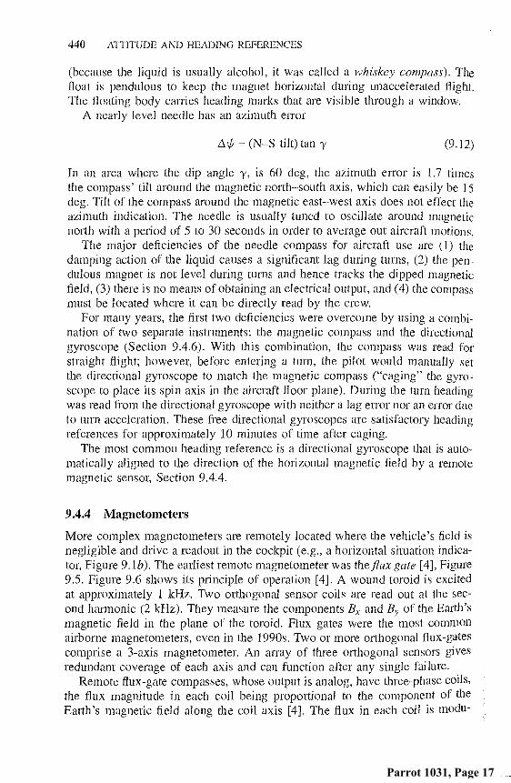
(because the liquid is usually alcohol, it was called a whiskey compass). The float is pendulous to keep the magnet horizontal during unaccelerated flight. The floating body carries heading marks that are visible through a window.

A nearly level needle has an azimuth error

= (N—S tilt) tan y (9.12)

In an area where the dip angle -y, is 60 deg, the azimuth error is 1.7 times the compass' tilt around the magnetic north—south axis, which can easily be 15 deg. Tilt of the compass around the magnetic east—west axis does not effect the azimuth indication. The needle is usually tuned to oscillate around magnetic north with a period of 5 to 30 seconds in order to average out aircraft motions.

The major deficiencies of the needle compass for aircraft use are (1) the damping action of the liquid causes a significant lag during turns, (2) the pen-dulous magnet is not level during turns and hence tracks the dipped magnetic field, (3) there is no means of obtaining an electrical output, and (4) the compass must be located where it can be directly read by the crew.

For many years, the first two deficiencies were overcome by using a combi-nation of two separate instruments: the magnetic compass and the directional gyroscope (Section 9.4.6). With this combination, the compass was read for straight flight; however, before entering a turn, the pilot would manually set the directional gyroscope to match the magnetic compass ("caging" the gyro-scope to place its spin axis in the aircraft floor plane). During the turn heading was read from the directional gyroscope with neither a lag error nor an error due to turn acceleration. These free directional gyroscopes are satisfactory heading references for approximately 10 minutes of time after caging.

The most common heading reference is a directional gyroscope that is auto-matically aligned to the direction of the horizontal magnetic field by a remote magnetic sensor, Section 9.4.4.

9.4.4 Magnetometers

More complex magnetometers are remotely located where the vehicle's field is negligible and drive a readout in the cockpit (e.g., a horizontal situation indica-tor, Figure 9.1b). The earliest remote magnetometer was the flux gate [4], Figure 9.5. Figure 9.6 shows its principle of operation [4]. A wound toroid is excited at approximately 1 kHz. Two orthogonal sensor coils are read out at the sec-ond harmonic (2 kHz). They measure the components B1 and By of the Earth's magnetic field in the plane of the toroid. Flux gates were the most common airborne magnetometers, even in the 1990s. Two or more orthogonal flux-gates comprise a 3-axis magnetometer. An array of three orthogonal sensors gives redundant coverage of each axis and can function after any single failure.

Remote flux-gate compasses, whose output is analog, have three-phase coils, the flux magnitude in each coil being proportional to the component of the Earth's magnetic field along the coil axis [4]. The flux in each coil is modu-

Parrot 1031,

By

y—sensing coil


Figure 9.5 Magnetic Flux Detector, Compass Engine, courtesy of KVH Industries, Inc.

dated as a result of an applied ac field from an excitation coil; this applied field causes saturation of the magnetic core of the coils at twice the frequency of the excitation. The three-phase winding is connected to the stator of a synchro receiver. A typical combination of remote magnetic sensor and receiver synchro will have errors of both one and two cycles per revolution, each of about 0.2 deg magnitude.

Earth's magnetic field

Approximately x-sensing 1—kHz excitation coil

Figure 9.6 Principle of flux gate magnetometer.

Parrot 1031,


The two-cycle error in the combined sensor and receiver—together with any soft-iron error due to the aircraft structure—can be corrected by adding proper impedances in series with the transmission wires. Such a correction is indepen-dent of the strength of the Earth's field.

The single-cycle instrument error is usually corrected together with the air-craft hard-iron error. However, this is not exact because the instrument error (in angular terms) is independent of the Earth's horizontal field—whereas the aircraft error is inversely proportional to the Earth's horizontal field (since the permanent magnet part of the aircraft's field is constant). In the 1990s, the trend was to do all corrections in the airborne computer.

Strapdown magnetometers came into use during the 1980s. The body-axis components of the Earth's field are

Hforward 1 0 0 Coos 0 0— sin 0

Hstarboard

{ = H 0 cos 0 sin q5 1 0

Hfloor 0— sin 0 cos 0 sin 0 0 cos 0

•

[

cos 0 sin 0 0 cos -y

— sin 0 cos 0 0 0 (9.13) 0 0 1 sin y

where 0, 0,1,G are the roll, pitch, and azimuth angles of the aircraft, respectively. These three body-axis components can be measured continuously. To solve for heading, Equation 9.13 is inversed:

{ cos — sin 0

0

sin 0

cos 0 0

0 0 1

cos y 0

sin -y (9.14a)

cos 0 0— sin 0 -1 1 { 0 0 0 1 0 0 cos 0 sin 1-1 [

(15 .0

Hforward I Hstarboard

sin 0 0 cos 0 0 — sin cos Hfloor

Therefore:

To solve for 0 in terms of

cos 11/ cosy — sin 0 cos yi

sin -y

the three body-axis

tan ;G = —

=

B

A B (9.14b) C

measurements,

(9.15)

where A and B are calculated from the measured body-axis components of the Earth's field. Hard iron is compensated in body-axes by subtracting 3 constants

H

Parrot 1031,


from the measured field. Soft iron is difficult to compensate, as explained in Section 9.4.3, so the magnetometer is best located far from structural iron.

For small roll and pitch angles, Equation 9.13 simplifies to

H forward cos -y cos \G — 0 sin -y

= cos -y sin IP+Osiny

H

H starboard

H

H

= tilt around E-W axis) cos y+ sin y

In that case, azimuth is computed easily subject to 0 and 43. errors:

tan (measured azimuth) = Hstarboard

Problem 9.6 shows that the heading error due to the magnetometer being off vertical is (north-south-axis tilt)* tan (magnetic dip).

In the 1980s, many small solid-state magnetometers became available with remote readouts for vehicle use [1]. They were based on the Hall, magnetostric-tive, and Faraday effects. Superconducting laboratory magnetometers have been too costly and complex for routine aircraft use. The most common heading ref-erence in the 1990s was a directional gyroscope (or AHRS) that is slaved to magnetic north by a remote magnetometer.

9.4.5 Electrical Swinging

Swinging is the process of compensating a compass at various headings. Small aircraft are swung by parking them at a succession of headings in an area free of construction iron. For large aircraft, electrical-swinging techniques have been developed that are as good as mechanical swinging.

The electrical-swinging technique depends on the fact that it is possible to create, at the remote magnetic sensor, a magnetic field of arbitrary magnitude and direction by passing direct currents through the sensor-output coils. It is thus possible to create a magnetic field at the sensor with an effect equivalent to that of rotating the sensor in the Earth's field. This requires good knowledge of the characteristics of the sensor and the strength of the local Earth's field. The required information is obtained by a preliminary test of the sensor out of the aircraft, followed by an electrical swing in the aircraft. Swinging must be done with electrical equipment "on" and "off" to correct for the magnetic fields of motors and wiring.

H floor = (0 cos 171/ + 4 sin lb) cos 7+ sin 7

Hforward

(9.16)

(9.17)

Parrot 1031,


Multisensor navigation systems can perform continuous swinging by recal-ibrating the magnetometer in level flight at many headings, as measured by the inertial sensor or a sequence of GPS fixes, for example. Reference [16) describes a Kalman filter for in-flight calibration of a compass. Continuous recalibration should account for the power-on status of electrical machinery and for newly installed magnetic materials.

9.4.6 The Directional Gyroscope

The directional gyroscope is a two degree-of-freedom device whose spin axis is nominally horizontal (Figure 9.7). The gimbal arrangement places the outer axis normal to the floor plane of the aircraft and the inner axis in the floor plane. Aircraft heading is read about the outer axis, and there is no data pickoff on the inner axis. A single electrolytic level is attached to the gyroscope housing to sense departure of the spin axis from a level condition; its output is applied to a torque motor on the outer axis. A torque motor is provided on the inner axis to precess the gyroscope about the outer axis for correction purposes and to slave the gyroscope to alignment with a remote magnetic sensor (if used). Figure 9.8 shows the application of magnetic slaving to a directional gyroscope. Some specific aspects of this design are as follows:

1. Since the inner axis is not used for indication, only drift about the outer axis is of importance. For this reason, the inner-axis-bearing design and adjustment are made to favor inner-axis torque (outer-axis drift).

2. Because mass unbalance along the spin axis results in drift about the outer axis, symmetry of the wheel and motor assembly is important. This is particularly true of instruments that may have to operate for long times without magnetic reference slaving.

3. Inner-axis gimbal bearings are sometimes designed so that the outer race

Gravity sensor

Figure 9.7 Elementary directional gyroscope.

Parrot 1031,

True heading

Sum Transmitter

Receiver

Magnetic heading sensor

Cutoff switch

Level

Torquer

rv—vm Cutoff switch

Torquer

Magnetic J I Magnetic heading variation

Figure 9.8 Directional gyroscope slaved to a magnetic sensor.


is kept rotating (either continuously or in an oscillatory manner) to reduce friction.

4. Because of the limited angle required and the great importance of inner-axis friction, center-of-rotation contacts are common for electrical con-nections across the inner axis, although slip rings must be used on the outer axis.

5. Multiple pancake synchros, one of which may be the receiver for a remote magnetic sensor, can be used on the outer axis. If several transmitters are needed, a heading-repeater servo or a single-heading transmitter and isolation amplifier is used.

Directional gyroscopes that are designed for continuous slaving to a remote magnetic sensor can have large free drift. For applications requiring extensive periods of unslaved operation, directional gyroscopes have been designed with a free drift of 0.25 deg/hr to 0.5 deg/hr over a wide range of temperatures.

When sustained operation without magnetic slaving is required, proper account must be taken of the vertical component of the Earth's rate and the air-craft's motion over the Earth. These effects are fully compensated in an inertial navigator and partially compensated in an AHRS.

In nonlevel flight, the outer-gimbal-axis torque may have a component that is in the horizontal plane and normal to the gyroscope spin axis. This torque

Parrot 1031,


component will cause drift about the vertical axis. For this reason, it is desirable to cut off the spin-axis leveling loop during turns. The error is at twice the frequency of angular vibration with peak magnitude of X2/4, where X is the departure, in radians, of the outer-gimbal axis from the vertical. The peak error is about 10 for a tilt of 15 deg. The slaving of a directional gyroscope to a remote magnetic sensor is accomplished by using acceleration smoothing similar to that discussed in Section 9.3.1.

9.5 INITIAL ALIGNMENT OF HEADING REFERENCES

Heading references are aligned by the following methods:

1. By reference to the Earth's magnetic field (Sections 9.4.4 and 9.4.6). 2. Use of a transfer gyroscope. This is a portable, low-drift gyroscope that

can be aligned to a surveyed north line and then carried aboard the aircraft as a heading reference to allow setting the installed directional reference. Accuracies on the order of 0.1 deg have been attained in this way. Alter-natively, the transfer gyroscope can itself be fastened into the aircraft for use in flight.

3. Alignment relative to the known runway heading prior to and during the takeoff run. Accuracy better than 0.5 deg has been attained by this method.

4. An astrocompass (Chapter 12) can reset the directional gyro. This tech-nique was widely used from 1930 to 1970.

5. Heading can be transferred from an inertial navigator to a directional gyro.

9.6 FUTURE TRENDS

Self-contained vertical gyroscopes, directional gyroscopes, and magnetometers will continue to be used on small aircraft, including target drones and unmanned aerial vehicles. They will continue to be used on larger aircraft as backup instru-ments for emergency use. In large commercial and military aircraft, the inertial navigation system (Chapter 7) will continue to be the source of attitude and heading information to the electronic displays and flight-management system.

Micro-machined gyros and accelerometers will probably be packaged as self-contained vertical and heading references, resulting in ultra-compact AHRS designed to operate with external sensors (Doppler, GPS, magnetometer). With the growing use of GPS, low-performance inertial navigators will overlap atti-tude and heading references in civil aircraft and in military aircraft that do not deliver weapons. In many military helicopters, AHRS will continue to be the heading and attitude reference for Doppler navigation radars (Chapter 10). Three-axis strapdown magnetometers will increasingly serve as the abso-

Parrot 1031,

PROBLEMS 447

lute heading source for simple AHRS, perhaps backing up GPS' indication of ground track angle. The search for lower-cost, more reliable 3-axis gyros, accelerometers, and magnetometers will continue. The growth of data bases will parallel the expansion of aviation into the Southern Hemisphere.

Higher-order magnetic models, supplemented by tables of local anomalies, will come into use as more magnetic data are collected worldwide. When intermittent-fix corn-nav satellites come into use in the twenty-first century, they will motivate the re-introduction of precise inertial navigators.

PROBLEMS

9.1 An aircraft directional gyroscope has an angular momentum of 10 million gram-cm2/sec, and the wheel weighs 500 grams. What stability of axial positioning of the wheel is required to obtain an acceleration-sensitive drift of 0.25 deg/hr-g.

Ans.: 2.5 x 10-5 cm.

9.2 An aircraft is maneuvering in such a way that its horizontal acceleration is 20 ft/sec2 and its vertical acceleration is —10 ft/sec2 (downward). What is the departure of the apparent vertical from the true vertical?

Ans.: 42 deg.

9.3 A vertical gyro is to be constructed using a wheel whose angular momen-tum is 107 gram-cm2/sec, a gravity sensor with a sensitivity of 0.5 volt/deg, and a coil that provides 5 x 103 dyne-cm of torque per volt applied. What voltage gain is required in an amplifier between the gravity sensor and torquer to yield a 1-min leveling-time constant?

Ans.: 1.12,

9.4 It is desired that the response of a second-order vertical reference to a peak sinusoidal horizontal acceleration of 2 ft/sec2 at a period of 15 sec not exceed 0.05 deg. It is also desired that the leveling be critically damped. What should the response time constant for the gravity sensor be? What should the leveling-loop time constant be? (HINT: first determine the ratio of the time constants for critical damping.)

Ans.: 0.165 min; 0.66 min.

9.5 Under the flight condition of Problem 9.4, it is desired that the directional gyro slaving error due to the acceleration not exceed 0.1 deg for the worst heading and at a latitude giving a dip angle of 60 deg. What time constant is required in a first-order slaving loop?

Ans.: 2.45 min.

Parrot 1031,


9.6 For small roll and pitch, differentiate Equation 9.17 with respect to roll and pitch to show that:

O~G=(0cos — 0 sin 1,G) tan 1,

Show that the expression in parentheses is the component of the magne-tometer's tilt-angle around the north-south axis.

Parrot 1031,

avionics navigation systems - microsoft. 1031.pdfavionics navigation systems second edition myron...

Documents