azim ataollahi oshkourstudentsrepo.um.edu.my/7574/1/azim_ataollahi_oshkour...azim ataollahi oshkour...
TRANSCRIPT

UTILIZATION OF FUNCTIONALLY GRADED MATERIALS IN FEMORAL PROSTHESIS
AZIM ATAOLLAHI OSHKOUR
FACULTY OF ENGINEERING
UNIVERSITY OF MALAYA
KUALA LUMPUR
2015

UTILIZATION OF FUNCTIONALLY GRADED MATERIALS IN FEMORAL PROSTHESIS
AZIM ATAOLLAHI OSHKOUR
THESIS SUBMITTED IN FULFILMENT OF THE REQUIREMENTS FOR THE DEGREE OF DOCTOR OF
PHILOSOPHY
FACULTY OF ENGINEERING UNIVERSITY OF MALAYA
KUALA LUMPUR
2015

ii
To
My beloved parents, my wife, my sisters, and my brother for their endless love, support, and encouragement

iii
UNIVERSITI MALAYA ORIGINAL LITERARY WORK DECLARATION
Name of Candidate: Azim Ataollahi Oshkour (I.C/Passport No: F16425429) Registration/Matric No: KHA10032 Name of Degree: Doctor of philosophy Title of Project Paper/Research Report/Dissertation/Thesis (“this Work”): Utilization of functionally graded materials in femoral prosthesis Field of Study: Biomechanics I do solemnly and sincerely declare that: (1) I am the sole author/writer of this Work; (2) This Work is original; (3) Any use of any work in which copyright exists was done by way of fair dealing and for permitted purposes and any excerpt or extract from, or reference to or reproduction of any copyright work has been disclosed expressly and sufficiently and the title of the Work and its authorship have been acknowledged in this Work; (4) I do not have any actual knowledge nor do I ought reasonably to know that the making of this work constitutes an infringement of any copyright work; (5) I hereby assign all and every rights in the copyright to this Work to the University of Malaya (“UM”), who henceforth shall be owner of the copyright in this Work and that any reproduction or use in any form or by any means whatsoever is prohibited without the written consent of UM having been first had and obtained; (6) I am fully aware that if in the course of making this Work I have infringed any copyright whether intentionally or otherwise, I may be subject to legal action or any other action as may be determined by UM. Candidate’s Signature Date Subscribed and solemnly declared before, Witness’s Signature Date Name: Designation:

iv
ABSTRACT
Total hip replacement is a highly effective surgical operation that relieves pain
and restores the function of a degenerated hip joint. However, with the increasing
incidence of total hip replacements, particularly among young patients, and femoral
prosthesis implantation, implant designs should consider long-term survival and better
performance. Minimizing the mismatch between the prosthesis and bone stiffness to
reduce stress shielding and retain interface stresses within acceptable levels, can
increase the longevity of total hip replacement and enhance the performance of the
prosthesis. A prosthesis with adjustable stiffness may enable prosthetists to match the
prosthesis and bone stiffness. Functionally graded materials have attracted much
attention in the production of prosthesis with customizable stiffness.
Computational modeling provides a flexible framework to examine the behavior
of hip replacements, host bone, and different implant design configurations using a
computer instead of conducting expensive and destructive experimental tests.
ABAQUS, a finite element software, was used to analyze a femur implanted with
different prostheses and determine the circumferential crack behavior in the cement
layer of a total hip replacement. The cemented and cementless Charnley femoral
prostheses composed of functionally graded materials were initially examined. Finite
element analysis was performed on the implanted femur with prostheses made of
conventional materials, such as stainless steel, and titanium alloys. Finite element
analysis was then conducted on the cementless and cemented functionally graded
femoral prostheses with different geometries. Circumferential cracks were located in the
cement layer on the internal and external surfaces of the cement at different positions
along its length from distal to proximal direction. After numerical studies, an
experiment was performed using the composites and functionally graded materials

v
composed of four metallic phases and two ceramic phases. Physical and compressive
mechanical properties were then examined.
Results revealed that a prosthetic material plays a key role on the strain energy
density in the proximal metaphysics of the femur and on the stress distribution in the
implanted femur constituents. Low-stiffness prostheses resulted in higher strain energy
density in the periprosthetic femur. In the femur with functionally graded prostheses,
strain energy density proportionally increased with gradient index growth. Stiffer
prostheses carried more stress than less stiff prostheses. The increase in gradient index
also showed an adverse relationship with the developed stress in the femoral prostheses.
However, the developed stress in the bone and cement demonstrated an increasing trend
with the increase in gradient index. The internal and external circumferential cracks had
no significant interaction. The numerical study on the circumferential crack behavior
revealed that KII was smaller than KI and KIII. Higher values of stress intensity factors
were obtained at the distal part compared with that at the proximal part of the cement
layer. Moreover, experimental results revealed that the abundant metallic and ceramic
composites showed better mechanical properties than those of the composites with 40
wt%–60 wt% of the metal and ceramic phases. In addition, compared to pure metals, the
functionally graded materials exhibited better mechanical properties, such as low
Young’s modulus. Functionally graded materials also demonstrated more compressive
stress and plastic deformation than the composites with more than 30 wt% ceramic
phases.

vi
ABSTRAK
Penggantian pinggul sepenuhnya adalah pembedahan yang amat efektif dalam
megurangkan kesakitan dan memulihkan fungsi sendi pinggul yang rosak. Walau
bagaimanapun, dengan merirgketnga kes penggantian pinggul sepenuhnya, terutamanya
di kalangan pesakit yang masih muda, dan implantasi prostesis tulang peha, reka bentuk
implan harus mempunyai jangka hayat yang panjang dan prestasi yang lebih baik.
Meminimumkan ketidakpadanan antara prostesis dan kekakuan tulang untuk
mengurangkan tegasan pelindung dan mengekalkan tegasan antara muka pada skala
yang boleh diterima akan meningkatkan jangka hayat implan penggantian pinggul
sepenuhnya dan meningkatkan prestasi prostesis. Prostesis dengan kekakuan boleh laras
membolehkan prostetis memadankan kekakuan prostesis dan tulang. Bahan bergred
fungsi telah menarik banyak perhatian dalam pengeluaran prostesis dengan kekakuan
boleh ubah suai.
Pemodelan berkomputer menyediakan satu rangka kerja yang fleksibel untuk
mengkaji sifat penggantian pinggul, tulang perumah, dan konfigurasi reka bentuk
implan yang berbeza dengan menggunakan komputer tanpa meggunakan ujian
eksperimen berkos tinggi dan merosakkan bahan. ABAQUS, iaitu perisian elemen
unsur, telah digunakan untuk menganalisis tulang paha yang diimplan dengan prostesis
yang berbeza dan menentakan keretakan lilitan dalam lapisan simen pada implan
penggantian pinggul sepenuhnya. Prostesis tulang paha Charnley, bersimen dan tanpa
simen, terdiri daripada bahan bergred fungsi, telah diperiksa. Analisis unsur terhingga
telah dijalankan ke atas tulang paha yang diimplan dengan prostesis yang diperbuat
daripada bahan-bahan konvensional seperti keluli tahan karat dan aloi titanium. Analisis
unsur terhingga kemudian dijalankan ke atas prosesis tulang peha tanpa simen dan
prosesis tulang peha bergred fungsi bersimen dengan geometri yang berbeza. Keretakan

vii
lilitan ditemui pada lapisan simen pada permukaan dalaman dan luaran simen di
kedudukan yang berbeza sepanjang jarak antara arah distal dan proksimal. Selepas
kajian numerikal, satu eksperimen telah dijalankan menggunakan komposit dan bahan-
bahan bergred fungsi yang terdiri daripada empat fasa dan dua fasa seramik. Sifat
mekanikal dan mampatan fizikal kemudiannya dikaji.
Hasil kajian menunjukkan bahawa bahan prostetik memainkan peranan penting
dalam ketumpatan tenaga terikan pada metafizik proksimal tulang paha dan agihan
teganan dalam juzuk tulang paha yang diimplan. Prostesis dengan kekakuan rendah
menyebabkan ketumpatan tenaga terikan yang lebih tinggi dalam tulang paha
periprostetik. Tulang paha dengan prosthesis bergred fungsi, mempunyai ketumpatan
tenaga terikan berkadaran meningkat secara berkadaram dengan kenaikan indeks
kecerunan. Prostesis yang lebih kaku mempunyai tegasan yang lebih berbanding
prostesis kurang kaku. Peningkatan indeks kecerunan juga menunjukkan hubungan
yang bertentangan dengan tegasan yang dihasilkan dalam prostesis tulang peha. Walau
bagaimanapun, tekanan yang terhasil dalam tulang dan simen menunjukkan trend yang
meningkat dengan peningkatan indeks kecerunan. Keretakan lilitan dalaman dan luaran
tidak mempunyai interaksi yang signifikan. Kajian numerikal ke atas kelakuan retak
lilitan mendedahkan bahawa KII adalah lebih kecil daripada KI dan KIII. Nilai faktor
keamatan tegasan yang lebih tinggi diperoleh di bahagian distal berbanding dengan di
bahagian proksimal lapisan simen. Tambahan pula, hasil eksperimen menunjukkan
bahawa koposit mewah logam dan seramik menunjukkan sifat-sifat mekanikal yang
lebih baik berbanding komposit dengan 40 wt% - 60 wt% logam dan fasa seramik. Di
berbaring dengan logen tuten, samping itu, bahan-bahan bergred fungsi menunjukkan
sifat mekanikal yang lebih baik, seperti modulus Young yang rendah, untuk implan.
Fungsi bahan gred juga menunjukkan lebih tengasan mampatan dan perubahbentuken
plastik berbanding komposit dengan lebih daripada 30 wt% fasa seramik.
viii
ACKNOWLEDGMENTS
I would like to express my deep gratitude to my supervisors, namely, Professor Ir. Dr.
Noor Azuan Abu Osman and Associate Prof. Ir. Dr. Yau Yat Huang, for providing me
the opportunity to continue my PhD program. I am also very thankful for their tireless,
kind assistance, support, critical advice, encouragement, and suggestions during the
study and preparation of the thesis.
I would also like to express my gratitude to Associate Prof. Ir. Dr. Faris Tarlochan and
Dr. Sumit Pramanik for the practical experience and knowledge that they imparted to
this thesis. I truly appreciate the time they devoted in advising me and showing me the
proper direction to continue my research and for their openness, honesty, and sincerity.
I am also thankful to Mr. Mohd Said Bin Sakat, technician of the Department of
Mechanical Engineering, Faculty of Engineering, University of Malaya, for his
willingness to provide assistance and advice as well as for being my friend.
ix
TABLE OF CONTENTS
ABSTRACT .................................................................................................................... iv
ABSTRAK ...................................................................................................................... vi
ACKNOWLEDGMENTS ........................................................................................... viii
TABLE OF CONTENTS ............................................................................................... ix
LIST OF FIGURES ...................................................................................................... xv
LIST OF TABLES ........................................................................................................ xx
CHAPTER 1 .................................................................................................................... 1
INTRODUCTION ........................................................................................................... 1
1.1 Introduction ........................................................................................................... 1
1.2 Problem statement ................................................................................................. 2
1.3 Objectives .............................................................................................................. 3
1.4 Thesis layout ......................................................................................................... 4
CHAPTER 2 .................................................................................................................... 5
LITERATURE REVIEW ............................................................................................... 5
2.1 Introduction ........................................................................................................... 5
2.2 Hip biomechanics .................................................................................................. 5
2.3 Total hip replacement ............................................................................................ 6
2.4 Implant fixation methods ...................................................................................... 8
2.5 Total hip replacement failure .............................................................................. 10
2.5.1 Osteolysis .................................................................................................... 10
2.5.2 Primary stability .......................................................................................... 11
2.5.3 Stress shielding ........................................................................................... 12
2.5.4 Cement failure ............................................................................................. 13
2.5.5 Debonding ................................................................................................... 14

x
2.5.6 Implant fracture ........................................................................................... 14
2.6 Material and geometry of artificial hip joint constituents ................................... 15
2.6.1 Femoral head and acetabular cup ................................................................ 15
2.6.2 Femoral prosthesis (Stem) .......................................................................... 17
2.6.3 Femoral prosthesis geometry ...................................................................... 17
2.6.4 Femoral prosthesis materials ....................................................................... 19
2.7 Surface finishing ................................................................................................. 20
2.8 Materials utilized in artificial hip joint components ........................................... 20
2.8.1 Metals .......................................................................................................... 20
2.8.2 Polymers ...................................................................................................... 21
2.8.3 Ceramics ...................................................................................................... 21
2.8.4 Composites .................................................................................................. 24
2.9 Numerical methods in hip joint biomechanics and implant study ...................... 26
2.10 Load transfer in the proximal femur ............................................................... 31
2.11 Bone ................................................................................................................ 33
2.12 Summary ......................................................................................................... 34
CHAPTER 3 .................................................................................................................. 35
MATERIALS AND METHODS ................................................................................. 35
3.1 Introduction ......................................................................................................... 35
3.2 Outline of Methodology ...................................................................................... 35
3.3 Finite element analysis ........................................................................................ 35
3.3.1 Finite element modeling to use functionally graded materials in femoral
prosthesis ................................................................................................................. 35
3.3.2 Bone modeling ............................................................................................ 38
3.3.3 Prosthesis modeling .................................................................................... 40
3.3.4 Mesh generation .......................................................................................... 42

xi
3.3.5 Boundary conditions ................................................................................... 42
3.3.6 Material properties ...................................................................................... 42
3.3.7 Functionally graded material modeling ...................................................... 43
3.3.8 Crack modeling ........................................................................................... 45
3.3.9 Validation of finite element models ............................................................ 46
3.4 Experimental procedure ...................................................................................... 47
3.4.1 Test Material ............................................................................................... 48
3.4.2 Composite powder preparation ................................................................... 48
3.4.3 Test specimen preparation........................................................................... 49
3.4.4 Structure characterization............................................................................ 49
3.4.5 Physical characterization ............................................................................. 50
3.4.6 Mechanical characterization........................................................................ 50
3.4.6.1 Vickers hardness test ........................................................................... 50
3.4.6.2 Compressive static test ........................................................................ 51
3.5 Summary ............................................................................................................. 52
CHAPTER 4 .................................................................................................................. 53
RESULTS ...................................................................................................................... 53
4.1 Introduction ......................................................................................................... 53
4.2 Finite element analysis ........................................................................................ 54
4.2.1 Longitudinal, radial, and longitudinal–radial FG Charnley femoral
prostheses ................................................................................................................ 56
4.2.1.1 Strain energy density ........................................................................... 56
4.2.1.2 Femoral prosthesis stress .................................................................... 60
4.2.1.3 Developed stress in the bone ............................................................... 64
4.2.1.4 Developed stress in the cement ........................................................... 67
4.2.1.5 Interface stresses ................................................................................. 70
xii
4.2.2 Cementless prostheses with conventional materials ................................... 72
4.2.2.1 Strain energy density ........................................................................... 72
4.2.2.2 Developed stress in the prostheses ...................................................... 74
4.2.2.3 Developed stress to the bone ............................................................... 76
4.2.3 Cementless longitudinal functionally graded femoral prosthesis with
different geometries ................................................................................................ 79
4.2.3.1 Strain energy density ........................................................................... 79
4.2.3.2 Prostheses stress .................................................................................. 81
4.2.3.3 Bone Stress .......................................................................................... 84
4.2.3.4 Interface stress ..................................................................................... 88
4.2.4 Cementless radial functionally graded femoral prosthesis with different
geometries ............................................................................................................... 90
4.2.4.1 Strain energy density ........................................................................... 90
4.2.4.2 Developed stress in prostheses ............................................................ 92
4.2.4.3 Developed stress in the bone ............................................................... 94
4.2.4.4 Interface Stress .................................................................................... 98
4.2.5 Cemented prostheses with conventional materials ................................... 101
4.2.5.1 Strain energy density ......................................................................... 101
4.2.5.2 Developed stress in the prostheses .................................................... 103
4.2.5.3 Developed stress in the bone ............................................................. 104
4.2.5.4 Developed stresses in the cement layer ............................................. 108
4.2.6 Radial and longitudinal cemented functionally graded prostheses ........... 111
4.2.6.1 Strain energy density ......................................................................... 111
4.2.6.2 Developed stress in the prostheses .................................................... 114
4.2.6.3 Developed stress in the bone ............................................................. 116
4.2.7 Developed stress in the cement ................................................................. 119

xiii
4.2.8 Circumferential cracks in cement.............................................................. 124
4.2.8.1 Internal circumferential crack ........................................................... 124
4.2.8.1.1 KI behavior .................................................................................... 124
4.2.8.1.2 KII behavior ................................................................................... 126
4.2.8.1.3 KIII behavior .................................................................................. 126
4.2.8.2 External circumferential crack .......................................................... 128
4.2.8.2.1 KI Behavior ................................................................................... 128
4.2.8.2.2 KII behavior ................................................................................... 129
4.2.8.2.3 KIII behavior .................................................................................. 129
4.2.8.3 Internal–external circumferential crack ............................................ 130
4.2.8.3.1 KI behavior at the internal and external surfaces .......................... 131
4.2.8.3.2 KIII behavior at the internal and external surfaces ........................ 135
4.3 Experimental results .......................................................................................... 140
4.3.1 Composite of calcium silicate and hydroxyapatite with metal phases ...... 140
4.3.1.1 Structure characterization.................................................................. 140
4.3.1.2 Physical properties ............................................................................ 147
4.3.1.3 Mechanical properties of the composites .......................................... 151
4.3.2 Functionally graded materials ................................................................... 154
4.3.2.1 Physical properties ............................................................................ 154
4.3.2.2 Mechanical properties ....................................................................... 155
CHAPTER 5 ................................................................................................................ 157
DISCUSSION .............................................................................................................. 157
5.1 Introduction ....................................................................................................... 157
5.2 Finite element analysis on the utilization of functionally graded material in
femoral prosthesis design .......................................................................................... 157
5.3 Existence of circumferential crack in the cement layer .................................... 162

xiv
5.4 Composites and functionally graded materials ................................................. 164
CHAPTER 6 ................................................................................................................ 166
CONCLUSION AND RECOMMENDATIONS ...................................................... 166
6.1 Conclusions ....................................................................................................... 166
6.2 Recommendations ............................................................................................. 168
LIST OF PUBLICATIONS ........................................................................................ 180
xv
LIST OF FIGURES
Figure 2.1: The hip joint (Stops et al., 2011) .................................................................... 6
Figure 2.2: Three typical hip joint diseases: (a) osteoarthritis, (b) necrosis, and (c) neck fracture (Dunne & Ormsby, 2011; Ilesanmi, 2010) .......................................................... 7
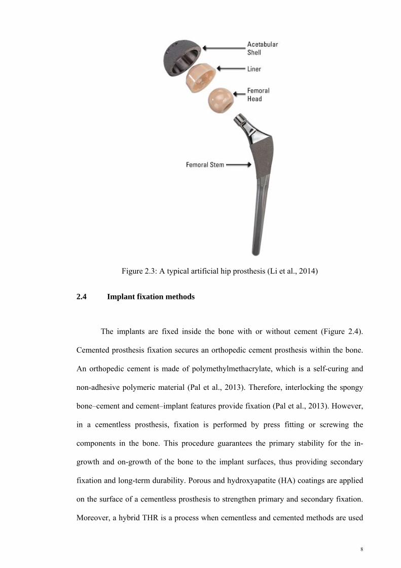
Figure 2.3: A typical artificial hip prosthesis (Li et al., 2014) .......................................... 8
Figure 2.4: Typical cemented and uncemented fixation (Izzo, 2012)............................... 9
Figure 2.5: Osteolysis after total hip replacement replacement (Bourghli et al., 2010) . 11
Figure 2.6: Load transfer before and after total hip replacement (Joshi et al., 2000) ..... 13
Figure 2.7: Fractures in a ceramic ball and acetabulum cup (Jenabzadeh et al., 2012) .. 14
Figure 2.8: Typical femoral heads and acetabulum cups (Heimann, 2010).................... 16
Figure 2.9: A typical total hip replacement (Jun & Choi, 2010)..................................... 17
Figure 2.10: Typical prosthesis geometries with different cross sections and profiles (Ramos et al., 2012) ........................................................................................................ 18
Figure 2.11: Schematic illustration of the different classifications of the cementless femoral stem designs. Type 1 is a single wedge, Type 2 is a double wedge, Type 3A is tapered and round, Type 3B is tapered and splined, Type 3C is tapered and rectangular, Type 4 is cylindrical and fully coated, Type 5 is modular, and Type 6 is anatomic. P = posterior and A = anterior (Khanuja et al., 2011) ........................................................... 19
Figure 2.12: Scheme of the aging process (Chevalier, 2006) ......................................... 24
Figure 2.13: A typical FGM structure: (a) gradient and (b) graded ................................ 26
Figure 2.14: Minimum and maximum principal stress distributions on the (a) lateral and (b) medial sides of the stem as a function of the prosthesis Young’s modulus (El-Sheikh et al., 2002) ...................................................................................................................... 27
Figure 2.15: A femoral prosthesis with metal core and variable stiffness (Simões & Marques, 2005) ............................................................................................................... 28
Figure 2.16: Hollow stems introduced by Gross and Abel (Gross & Abel, 2001) ......... 29
Figure 2.17: Different cross-sections and profiles (Bennett & Goswami, 2008; Sabatini & Goswami, 2008) .......................................................................................................... 30
Figure 2.18: Stem geometry developed by Ramos et al. (2012) ..................................... 30
Figure 2.19: Principles of the load transfer mechanism explained with a simplified intrameduilary fixation model (Huiskes, 1988) .............................................................. 32

xvi
Figure 2.20: Bone structure (Juillard, 2011) ................................................................... 33
Figure 3.1: General description of the methodology adopted in the study ..................... 36
Figure 3.2: General description of the finite element analysis adopted in the study ...... 37
Figure 3.2: Development of the three-dimensional model of the femur using Mimic® software ........................................................................................................................... 39
Figure 3.3: Three-dimensional models of the femur: (a) anatomical and (b) simplified 39
Figure 3.4: Stem models developed using Solidworks ................................................... 40
Figure 3.5: Dimensions of (a) profile, (b) proximal cross-sections, and (c) distal cross-sections ............................................................................................................................ 41
Figure 3.7: Internal crack geometry and locations of crack in the cement layer at (a) 25, (b) 50, (c) 75, and (d) 100 mm ........................................................................................ 46
Figure 3.8: Flowchart of the experimental procedure ..................................................... 47
Figure 3.9: Typical testing of sample .............................................................................. 49
Figure 3.10: A micro-hardness tester machine ............................................................... 51
Figure 3.11: An Instron universal testing machine ......................................................... 51
Figure 4.1: Flow chart of result presentation .................................................................. 55
Figure 4.2: Strain energies in the spongy portion of the proximal metaphysis of the femur caused by implantation of (a) normal walking–cemented, (b) normal walking–non-cemented, (c) stair climbing–cemented, and (d) stair climbing–non-cemented prostheses. (The legend shows the changes in the radial volume fraction gradient exponent) ......................................................................................................................... 59
Figure 4.3: Variation in the von Mises stress in the prosthesis as a function of volume fraction gradient exponent in the non-cemented (a) longitudinal and (b) radial prostheses ........................................................................................................................ 61
Figure 4.4: Stress variations in the longitudinal femoral prosthesis during normal walking at the (a) lateral and (b) medial sides of cemented prosthesis as well as at the (c) lateral and (d) medial sides of the cementless prosthesis .......................................... 61
Figure 4.5: Stress variation in the longitudinal femoral prosthesis in stair climbing at the (a) lateral and (b) medial sides of the cemented prosthesis as well as at the (c) lateral and (d) medial sides of the cementless prosthesis ........................................................... 62
Figure 4.6: Stress variation in the femur during normal walking. (a) Maximum principal stress and cemented prosthesis, (b) minimum principal stress and cemented prosthesis, (c) maximum principal stress and cementless prosthesis, and (d) minimum principal stress and cementless prosthesis...................................................................................... 65

xvii
Figure 4.7: Stress variation in the femur during stair climbing. (a) Maximum principal stress and cemented prosthesis, (b) minimum principal stress and cemented prosthesis, (c) maximum principal stress and cementless prosthesis, and (d) minimum principal stress and cementless prosthesis...................................................................................... 66
Figure 4.8: Stress variation in the cement layers during normal walking [(a) internal and (b) external layers] and stair climbing [(c) internal and (d) external layers] .................. 68
Figure 4.9: Stress variation in the cement layers during normal walking [(a) internal and external layers] and stair climbing [(c) internal and (d) external layers] ........................ 69
Figure 4.10: Strain energy density as a function of (a) distal cross section, (b) proximal cross section, (c) profile, and (d) material composition .................................................. 73
Figure 4.11: Variation in the mean von Mises stress variation as a function of (a) distal cross section, (b) proximal cross section, (c) profile, and (d) material composition ...... 75
Figure 4.12: Variation in the mean maximum principal stress as a function of (a) distal cross section, (b) proximal cross section, (c) profile, and (d) material composition ...... 77
Figure 4.13: Variation in the mean minimum principal stress variation as a function of (a) distal cross section, (b) proximal cross section, (c) profile, and (d) material composition ..................................................................................................................... 78
Figure 4.14: Variation in the mean strain energy variation for the different (a) distal cross-sections, (b) proximal cross-sections, (c) profiles, (d) interface properties, and (e) gradient indices ............................................................................................................... 81
Figure 4.15: Variation in the mean von Mises for the different (a) distal cross-sections, (b) proximal cross-sections, (c) profiles, (d) interface properties, and (e) gradient indices ......................................................................................................................................... 83
Figure 4.16: Variation in the mean maximum principal stress for the different (a) distal cross-sections, (b) proximal cross-sections, (c) profiles, (d) interface properties, and (e) gradient indices ............................................................................................................... 86
Figure 4.17: Variation in the mean minimum principal stress for the different (a) distal cross-sections, (b) proximal cross-sections, (c) profiles, (d) interface properties, and (e) gradient indices ............................................................................................................... 88
Figure 4.18: Variation in the mean interface stress for the different (a) distal cross-sections, (b) proximal cross-sections, (c) profiles, and (d) gradient indices ................... 90
Figure 4.19: Variation in the strain energy density a function of (a) distal cross-section, (b) proximal cross-section, (c) profile, and (d) gradient index ....................................... 92
Figure 4.20: Variation in the von Mises stress as a function of (a) distal cross-section, (b) proximal cross-section, (c) profile, and (d) gradient index ....................................... 94
Figure 4.21: Variation in the maximum principal stress as a function of (a) distal cross-section, (b) proximal cross-section, (c) profile, and (d) gradient index .......................... 96

xviii
Figure 4.22: Variation in the minimum principal stress as a function of (a) distal cross-section, (b) proximal cross-section, (c) profile, and (d) gradient index .......................... 97
Figure 4.23: Variation in the interface stress as a function of (a) distal cross-section, (b) proximal cross-section, (c) profile, and (d) gradient index ........................................... 100
Figure 4.24: Strain energy density as a function of the (a) distal cross-section, (b) proximal cross-section, (c) profile, and (d) material of the prostheses ......................... 102
Figure 4.25: Variation in the mean von Mises stress as a function of the (a) distal cross-section, (b) proximal cross-section, (c) profile, and (d) material of the prostheses ...... 104
Figure 4.26: Variation in the mean maximum principal stress as a function of the (a) distal cross-section, (b) proximal cross-section, (c) profile, and (d) material of the prostheses ...................................................................................................................... 106
Figure 4.27: Variation in the mean minimum principal stress as a function of the (a) distal cross-section, (b) proximal cross-section, (c) profile, and (d) material of the prostheses ...................................................................................................................... 107
Figure 4.28: Variation in the mean maximum principal stress as a function of the (a) distal cross-section, (b) proximal cross-section, (c) profile, and (d) material of the prostheses ...................................................................................................................... 110
Figure 4.29: Variation in the mean minimum principal stress as a function of the (a) distal cross-section, (b) proximal cross-section, (c) profile, and (d) material of the prostheses ...................................................................................................................... 111
Figure 4.30: Variation in the strain energy density at the different (a) distal cross-sections, (b) proximal cross-sections, (c) profiles, and (d) gradient indices ................. 113
Figure 4.31: Variation in the von Mises stress in various femoral prosthesis type and side at the different (a) distal cross-sections, (b) proximal cross-sections, (c) profiles, and (d) gradient indices ................................................................................................. 115
Figure 4.32: Variation in the maximum principal stress at the lateral side of femur at the different (a) distal cross-sections, (b) proximal cross-sections, (c) profiles, and (d) gradient indices ............................................................................................................. 117
Figure 4.33: Variation in the minimum principal stress at the lateral side of the femur at the different (a) distal cross-sections, (b) proximal cross-sections, (c) profiles, and (d) gradient indices ............................................................................................................. 119
Figure 4.34: Variation in the maximum principal stress at the different (a) distal cross-sections, (b) proximal cross-sections, (c) profiles, and (d) gradient indices ................. 121
Figure 4.35: Variation in the minimum principal stress at the different (a) distal cross-sections, (b) proximal cross-sections, (c) profiles, and (d) gradient indices ................. 123
Figure 4.36: KI variation along the crack front length at different crack locations: (a) 25, (b) 50, (c) 75, and (d) 100 mm ...................................................................................... 125
xix
Figure 4.37: KII variations along the crack front length at different crack locations: (a) 25, (b) 50, (c) 75, and (d) 100 mm ................................................................................ 126
Figure 4.38: KIII variation along the crack front length at different crack locations: (a) 25, (b) 50, (c) 75, and (d) 100 mm ................................................................................ 127
Figure 4.39: KI variation along the crack front length at different crack locations: (a) 25, (b) 50, (c) 75, and (d) 100 mm ...................................................................................... 128
Figure 4.40: KII variation along the crack front length at different crack locations (a) 25, (b) 50, (c) 75, and (d) 100 mm ...................................................................................... 129
Figure 4.41: KIII variations along the crack front length at different crack locations: (a) 25, (b) 50, (c) 75, and (d) 100 mm ................................................................................ 130
Figure 4.42: KI variation along the crack front on the internal surface: (a) I25, (b) I50, (c) I75, and (d) I100 interactions with E25, E50, E75, and E100 ................................................ 133
Figure 4.43: KI variation along the crack front on the internal surface: (a) E25, b) E50, (c) E75, and (d) E100 interactions with I25, I50, I75, and I100 .................................................. 135
Figure 4.44: KIII variation along the crack front on the internal surface: (a) I25, (b) I50, (c) I75, and (d) I100 interactions with E25, E50, E75, and E100 ................................................ 137
Figure 4.45: KIII variation along the crack front on the internal surface: (a) E25, (b) E50, (c) E75, and (d) E100 interactions with I25, I50, I75, and I100 ............................................ 139
Figure 4.46: X-ray diffraction patterns of the CaSiO3–Ti sintered composites ............ 141
Figure 4.47: X-ray diffraction patterns of CaSiO3–Ti–55Ni sintered composites ........ 142
Figure 4.48: X-ray diffraction patterns of CaSiO3–Ti–6Al–4V sintered composites ... 143
Figure 4.49: X-ray diffraction patterns of CaSiO3–SS–316L sintered composites ...... 144
Figure 4.50: X-ray diffraction patterns of Ca10(OH)2(PO4)6–Ti sintered composites .. 145
Figure 4.51: X-ray diffraction patterns of Ca10(OH)2(PO4)6–TI–6Al–4V sintered composites ..................................................................................................................... 146
Figure 4.52: XRD patterns of Ca10(OH)2(PO4)6–SS–316L sintered composites .......... 147
Figure 4.53: Variation in shrinkage as a function of weight percentages of (a) calcium silicate and (b) hydroxyapatite ...................................................................................... 148
Figure 4.54: Variation in density as a function of the weight percentages of (a) calcium silicate and (b) hydroxyapatite ...................................................................................... 149
Figure 4.55: Vickers hardness variation as a function of weight percentages of (a) calcium silicate and (b) hydroxyapatite ........................................................................ 151

xx
LIST OF TABLES
Table 3.1: CT scan slices ................................................................................................ 38
Table 3.2: Material properties of the implanted femur components ............................... 43
Table 3.3: Weight percentages of raw powders in the composites ................................. 48
Table 4.1: von Mises stress on femoral prosthesis (MPa) .............................................. 64
Table 4.2: Maximum and minimum principal stresses on the femur (MPa). ................. 67
Table 4.3: Maximum principal stress on the cement (MPa) ........................................... 70
Table 4.4: Interface stresses in cemented prosthesis (MPa) ........................................... 71
Table 4.5: Variation in Young’s modulus as a function of calcium silicate weight percentage ..................................................................................................................... 152
Table 4.6: Young’s modulus variation as a function of hydroxyapatite weight percentage ..................................................................................................................... 152
Table 4.7: Ultimate compressive strength as a function of calcium silicate weight percentage ..................................................................................................................... 153
Table 4.8: Ultimate compressive strength as a function of hydroxyapatite weight percentage ..................................................................................................................... 153
Table 4.9: Strain percentage at maximum load as a function of calcium silicate weight percentage ..................................................................................................................... 154
Table 4.10: Strain percentage at maximum load as a function of hydroxyapatite weight percentage ..................................................................................................................... 154
Table 4.11: Variation in shrinkage as a function of weight percentages of calcium silicate and hydroxyapatite ............................................................................................ 155
Table 4.12: Variation in density as a function of weight percentages of calcium silicate and hydroxyapatite ........................................................................................................ 155
Table 4.13: Compressive Young’s modulus as a function of weight percentages of calcium silicate and hydroxyapatite .............................................................................. 156
Table 4.14: Ultimate compressive strength as a function of weight percentages of calcium silicate and hydroxyapatite .............................................................................. 156
Table 4.15: Compressive strain percentage at maximum load as a function of weight percentages of calcium silicate and hydroxyapatite ...................................................... 156

xxi
LIST OF SYMBOLS AND ABBREVIATIONS
2D Two-dimensional
3D Three-dimensional
CMC Ceramic metal composite
CoC Ceramic-on-ceramic
CoP Ceramic-on-polyethylene
CS Calcium silicate
CT Computed tomography
FEA Finite element analysis
FEM Finite element method
FG Functionally graded
FGM Functionally graded material
HA Hydroxyapatite
LP Longitudinal prosthesis
LLP Lateral side of longitudinal prostheses
L-RP Longitudinal–radial prostheses
LRP Lateral side of radial femoral prostheses
MCC Metal ceramic composite
MLP Medial side of longitudinal prostheses
MoM Metal-on-metal
MoP Metal-on-polymer
MRP Medial side of radial prostheses
PTFE Polytetrafluoroethylene
RP Radial prosthesis
SED Strain energy density
SIF Stress intensity factor

xxii
St Stainless steel
STD Standard deviation
THR Total hip replacement
Ti Titanium
wt% Weight percentage
XRD X-ray diffraction

1
CHAPTER 1
1. INTRODUCTION
1.1 Introduction
Torturous pain and abnormality in hip joint function are outcomes of severe hip
joint degeneration or injury. The final recourse but effective procedure to release pain
and restore the normal function of the hip joint is total hip replacement (THR).
Fractured femoral neck, particularly in the elderly, avascular necrosis, osteoarthritis,
rheumatoid arthritis, and developmental dysplasia require THR. Although THR is an
operation with good success rate, failure does happen. THR failure in young patients
has become a serious problem because of the increasing incidence of revision surgeries.
Revision surgeries are complex and costly, but with poor results. Therefore, long-term
THR lifespan is the main goal in new prosthesis designs and serves as the motivation
for a prosthetist.
Artificial replacements of body organs demand materials with superior
characteristics because of the complex loading and chemical conditions of the human
body. Therefore, using composite materials has been increasingly popular. Functionally
graded materials (FGMs), which are special composite materials, exhibit interesting
properties which make them suitable substitutes for the current materials applied in hip
prosthesis. Moreover, loads are transferred from the natural hip joint between the pelvis
and the femur through the acetabulum to the head and neck of the femur. After THR,
loads are transferred through the prosthesis. An optimal prosthesis design should
transfer loads between the pelvis and the femur in a way similar to the natural hip joint
without causing extremely damaging peak stress or micromotion. Thus, the

2
performance of FGM-based prosthesis with different geometries was investigated in the
present study.
Experimental and numerical approaches should be used to evaluate the
performance of orthopedic implants containing FGMs. Mechanical testing of orthopedic
prostheses in vivo and in vitro provides valuable information for the preclinical
assessment of their performance. However, experimental methods are costly, time-
consuming, and destructive. On the other hand, numerical methods, such as the finite
element analysis (FEA), are common stress analysis approaches to examine complex
structures and design parameters without expensive prototyping. These methods are
particularly suitable for analyzing hip prostheses because in vivo testing would not be
required if the implant has a negative effect.
1.2 Problem statement
THR is the final recourse but effective procedure to relieve pain and restore the
function of a degenerated hip joint. However, THR has a limited lifespan, and revision
surgeries are complex with poor results. Therefore, prosthetists have developed new
types of prostheses to increase the durability of THR. Aseptic loosening compromises
the lifespan of failed THR. Stress shielding, interface stress, crack, and crack
propagation into the cement layer are the main causes of aseptic loosening. Therefore,
stress shielding and interface stress should be minimized to prolong the longevity of
THR. Additionally, crack behavior and propagation should be evaluated. Stress
shielding and interface stress are affected by prosthesis design (i.e., material and
geometry). The conventional materials [titanium (Ti), Ti alloys, chrome–cobalt (Cr–
Co), and stainless steel (St)] used in femoral prosthesis have conflicting effects on stress
shielding and interface stress. The conventional materials with lower Young’s modulus
3
induce more interface stress but cause less stress shielding. By contrast, the
conventional materials with higher Young’s modulus result in more stress shielding and
less interface stress. Therefore, the present study was designed to balance between stress
shielding and interface stress in order to prolong the lifespan of THR using FGMs in
constructing femoral prosthesis with different geometries. In addition, the behavior of
circumferential cracks at different positions in the cement layer was analyzed because of
the significant role of these cracks in aseptic loosening.
1.3 Objectives
The objectives of this study are as follows:
i. To evaluate the effects of gradient index and geometry of prosthesis on the
stimulated strain energy density (SED) in the proximal metaphysis of the
femur.
ii. To examine the effects of gradient index and geometry of prosthesis on the
developed stress in the prosthesis, bone, and cement as well as on the
interface stresses.
iii. To study the existence of circumferential cracks in the cement layer.
iv. To evaluate mechanical properties of the metal/ceramic composites,
ceramic/metal composites, and FGMs.

4
1.4 Thesis layout
This thesis is divided into six chapters. After the introductory chapter, chapter
two presents a critical review of relevant literature and focuses on hip joint
biomechanics, THR, failure of THR, and biomaterials. Chapter three outlines the
underlying theory and experimental techniques used in the current work, and the results
are presented in chapter four. Chapter five discusses the correlation between the
obtained results with the existing theory. Finally, chapter six provides the conclusion
and recommendations for future studies.
5
CHAPTER 2
2. LITERATURE REVIEW
2.1 Introduction
This chapter presents a brief review on the hip joint and THR. Hip
biomechanics, THR, implant fixation methods, THR failure, geometric functions, and
materials of the artificial hip joint components, biomaterials, and FEA are also
discussed in this chapter.
2.2 Hip biomechanics
The hip joint is composed of soft and hard tissues. A joint comprises the femoral
head, acetabulum, cartilage, and ligaments (Figure 2.1). The hip joint is classified as a
ball and socket joint (Polkowski & Clohisy, 2010). The ball and socket joint provides
three rotational movements, namely, flexion–extension, abduction–adduction, and
internal–external rotation. The femoral head is connected to the femur via the femoral
neck. The cartilage supplies a frictionless joint. The stability of the hip joint is supplied
by the ligaments and muscles. This structure provides an optimal stability for the stance
and bipedal locomotion, but the hip joint endures complex dynamic and static loads
(Bowman Jr et al., 2010).

6
Figure 2.1: The hip joint (Stops et al., 2011)
2.3 Total hip replacement
Mechanical injury, chemical process, and/or their combination can cause
degeneration and dysfunction in the articular hip joint (Bougherara et al., 2011). The
most common causes of hip joint degeneration are osteoarthritis, fracture of the hip,
inflammatory arthritis, femoral head necrosis, and rheumatoid arthritis (Figure 2.2).

7
Figure 2.2: Three typical hip joint diseases: (a) osteoarthritis, (b) necrosis, and (c) neck fracture (Dunne & Ormsby, 2011; Ilesanmi, 2010)
The final recourse but the most successful procedure to remedy severely
degenerated hip joint is THR (Caeiro et al., 2011). This procedure alleviates the pain
and restores the hip joint function. In THR, the natural hip joint is replaced with an
artificial hip joint, which consists of the femoral head, acetabular cup (acetabular shell
and liner), and femoral prosthesis (stem) (Figure 2.3). The artificial hip joint
components are formed in a modular or monoblock structure. A femoral head may also
be included in a femoral prosthesis in a monoblock structure.
(a) (b)
(c)
(a) (b)
(c)
8
Figure 2.3: A typical artificial hip prosthesis (Li et al., 2014)
2.4 Implant fixation methods
The implants are fixed inside the bone with or without cement (Figure 2.4).
Cemented prosthesis fixation secures an orthopedic cement prosthesis within the bone.
An orthopedic cement is made of polymethylmethacrylate, which is a self-curing and
non-adhesive polymeric material (Pal et al., 2013). Therefore, interlocking the spongy
bone–cement and cement–implant features provide fixation (Pal et al., 2013). However,
in a cementless prosthesis, fixation is performed by press fitting or screwing the
components in the bone. This procedure guarantees the primary stability for the in-
growth and on-growth of the bone to the implant surfaces, thus providing secondary
fixation and long-term durability. Porous and hydroxyapatite (HA) coatings are applied
on the surface of a cementless prosthesis to strengthen primary and secondary fixation.
Moreover, a hybrid THR is a process when cementless and cemented methods are used

9
to fix the artificial hip joint components in THR. Bone quality is the most influential
criterion in selecting a fixation procedure. Young and more active patients have better
bone quality than old and less active patients. Accordingly, a cementless prosthesis is
more appropriate for young patients, whereas a cemented prosthesis is more suitable for
older patients. Each implant fixation method has advantages and disadvantages. For
example, cement provides instant fixation, but a cementless prosthesis bone must grow
to secure the prosthesis in the bone. In addition, a cemented prosthesis requires a bigger
hole or more reaming inside the bone than cementless prostheses. The revision rate of
patients who underwent THR with cemented prosthesis is lower than that of patients
with cementless prosthesis.
Figure 2.4: Typical cemented and uncemented fixation (Izzo, 2012)

10
2.5 Total hip replacement failure
Developments in the design, technology, and technical operation increased the
success rate of THR. However, THR failure remains a problem, so revision surgery is
essential and unpreventable. For example, 10% of all THR surgeries in the USA per
year undergo THR revision surgery (Brown & Huo, 2002). Accordingly, the
components of the old artificial joint are partially or totally replaced with new
components. Mechanical factors are more common causes of THR failure than
infection. Aseptic loosening is the most important cause of THR failure (Gross & Abel,
2001). The mechanisms leading to aseptic loosening remain ambiguous. Osteolysis,
lack of sufficient primary stability, stress shielding, cement failure, and debonding are
some of the main factors that contribute to the development of aseptic loosening and
ultimately destruction of THR (Boyle & Kim, 2011; Sivarasu et al., 2011).
2.5.1 Osteolysis
The fretting of the THR joint components against each other releases debris in
the joint environment, and the released debris activate the immune system, which
causes bone resorption in a biological process known as osteolysis (Figure 2.5)
(Bourghli et al., 2010; Fabbri et al., 2011; Suárez-Vázquez et al., 2011). Osteolysis is
the main biological factor that causes aseptic loosening. Young patients have higher risk
of osteolysis than old patients because of their higher range of activities that release
more frictional debris (Beldame et al., 2009; Canales et al., 2010; Yoo et al., 2013).
Thus, engineers have developed new designs, coatings, alloys, and bearing surfaces to
cope with osteolysis (Canales et al., 2010). The risk of osteolysis in THR with
polyethylene component is higher than those with ceramic-on-ceramic (CoC) or metal-
on-metal (MoM) joints because of the size and amount of debris (Yoo et al., 2013). A
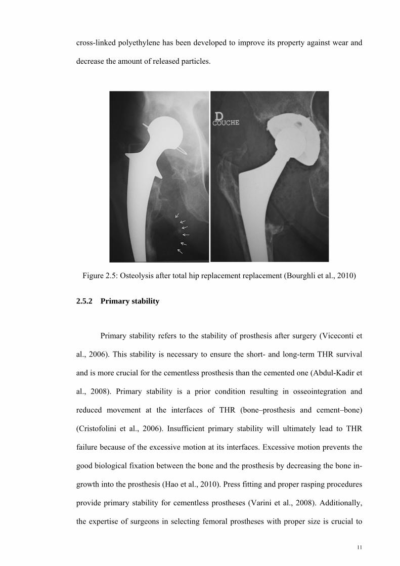
11
cross-linked polyethylene has been developed to improve its property against wear and
decrease the amount of released particles.
Figure 2.5: Osteolysis after total hip replacement replacement (Bourghli et al., 2010)
2.5.2 Primary stability
Primary stability refers to the stability of prosthesis after surgery (Viceconti et
al., 2006). This stability is necessary to ensure the short- and long-term THR survival
and is more crucial for the cementless prosthesis than the cemented one (Abdul-Kadir et
al., 2008). Primary stability is a prior condition resulting in osseointegration and
reduced movement at the interfaces of THR (bone–prosthesis and cement–bone)
(Cristofolini et al., 2006). Insufficient primary stability will ultimately lead to THR
failure because of the excessive motion at its interfaces. Excessive motion prevents the
good biological fixation between the bone and the prosthesis by decreasing the bone in-
growth into the prosthesis (Hao et al., 2010). Press fitting and proper rasping procedures
provide primary stability for cementless prostheses (Varini et al., 2008). Additionally,
the expertise of surgeons in selecting femoral prostheses with proper size is crucial to

12
achieve good primary stability (Varini et al., 2008). In vitro tests and numerical
methods have been employed to measure the primary stability of different femoral
prostheses (Viceconti et al., 2006). Moreover, intra-operative devices help surgeons to
immediately examine the prosthesis stability after surgery (Varini et al., 2008).
2.5.3 Stress shielding
The stress distribution in the femur at the hip joint is altered after implanting a
femoral prosthesis because load transfer changes from the joint to the bone as shown in
Figure 2.6 (Joshi et al., 2000). The change in stress distribution is due to the mismatch
between the prosthesis and bone stiffness (rigidity) (Behrens et al., 2008; Katoozian et
al., 2001). Thus, some portions of the bone in THR tolerate less stress compared with
the natural bone. This phenomenon is called stress shielding, and rigid prostheses can
shield more load transfer from the hip joint to the femur at the proximal metaphysis
(Gross & Abel, 2001). Contrary to engineering materials, the bone is a living tissue that
can adapt to its mechanical and chemical environment, and it loses its strength because
of load absence and stress shielding (Doblaré et al., 2004; Katoozian et al., 2001).
Accordingly, excessive stress can develop at the interface of the bone–prosthesis and
bone–cement (Gross & Abel, 2001) and cause aseptic loosening , which ultimately
results in THR collapse. Therefore, stress shielding should be minimized after THR and
stress distribution should be similar to the physiological condition to increase THR
durability (Behrens et al., 2008).

13
Figure 2.6: Load transfer before and after total hip replacement (Joshi et al., 2000)
2.5.4 Cement failure
Bone cement is a brittle material that provides stability and fixation to the
prostheses cemented to the host bone (Janssen et al., 2008; Lewis, 1997). Therefore,
cement layer failure results in aseptic loosening (Lai et al., 2009). The strengths of the
mechanical bone cement in compressive, tensile, and bending are 75 MPa – 105 MPa,
50 MPa – 60 MPa, and 65 MPa – 75 MPa, respectively. Moreover, the recommended
thickness of the cement layer in THR ranges from 2 mm to 5 mm, whereas the cement
layer with 5 mm–10 mm thickness is deleterious for the THR lifespan; more cracks are
also detected in thinner cement layer (Scheerlinck & Casteleyn, 2006). Cement endures
dynamic mechanical repetitive loadings during daily activities (De Santis et al., 2000),
and the amplitude of such loadings depends on the type of activity, such as walking,
running, or stair climbing. Cyclic loads cause fatigue, which accumulates in the cement
layer (Verdonschot & Huiskes, 1997). These loads cause crack initiation and
propagation (Waanders et al., 2011; Zivic et al., 2012). In addition, cracks could be
initiated during polymerization because of porosities or internal tension and then

14
propagated in the cement mantle caused by the fatigue loads of daily activities, which
ultimately result in cement failure (Achour et al., 2010; Zivic et al., 2012).
2.5.5 Debonding
Debonding at the interfaces is another factor that causes aseptic loosening and
THR failure. This condition can occur at the cement–prosthesis or cement–bone
interface, although most studies have shown the former case (Pérez et al., 2005).
Debonding at prosthesis–cement causes higher hoop cement stress and increases the
crack densities at the cement (Verdonschot & Huiskes, 1997).
2.5.6 Implant fracture
Fracture rarely occurs in the femoral component of THR. The number of
fractures in a cemented femoral prosthesis is higher than that in the cementless
prosthesis. However, fractures in the ceramic head and acetabulum cup are frequently
detected because of the brittleness of ceramics (Figure 2.7).
Figure 2.7: Fractures in a ceramic ball and acetabulum cup (Jenabzadeh et al., 2012)

15
2.6 Material and geometry of artificial hip joint constituents
The main factors in THR failure are briefly presented in previous sections.
Reducing the effect of these factors is the initial step to create a successful design of
artificial joint components. According to the literature, the geometry, materials, and
surface finishing of the prosthesis are the possible characteristics that should be adjusted
to achieve optimal designs. Therefore, the following sections briefly review the
materials used and the geometries of artificial hip joint constituents.
2.6.1 Femoral head and acetabular cup
After THR, the femoral head and acetabulum are replaced with MoM, metal-on-
polymer (MoP), ceramic-on-polyethylene (CoP), or CoC bearing couples (Figure 2.8).
The most commonly used couple joints are MoP and MoM (Catelas et al., 2011). The
main criteria for selecting the design and materials for the hip joint bearing are fracture
toughness, wear resistance, and frictional properties. Different bearings exhibit varying
strengths and weaknesses. In MoP and CoP couple joints, the polymer against ceramic
and metal is soft. Therefore, wear occurs in the polymer part of the joint couple. The
wearing of polymer and the release of debris into the joint environment primarily cause
joint luxation and osteolysis (Tudor et al., 2013). However, the developments in new
cross-linked polyethylene can decrease the wear rate and particle sizes (Catelas et al.,
2011). Moreover, in designing a process for the MoP couple joint to decrease friction,
the artificial femoral head size should be approximately 28 mm to 36 mm, which is
considerably smaller than the intact natural femoral head. MoM and CoC have been
developed to prevent the release of debris in the joint environment. The second
generation of the MoM joint couple with large head and low wear rate is more preferred
for THR than the first generation, which shows very weak performance because of the

16
poor design features and surgical techniques (Molli et al., 2011; Naudie et al., 2004).
Improving and optimizing metallurgical approaches (carbon content, method of
fabrication, and heat treatment) and geometries (clearance, sphericity, surface finish,
functional arc, fixation surface, and head size) enable the second generation of MoM to
be superior to the first generation (Molli et al., 2011). Regardless of these advances in
producing the MoM couple joint, its exposure to released metal ions because of the
articulation wear in the joint remains unsolved (Vendittoli et al., 2011). Thus, CoC
couple joints, which have outstanding wear resistance, have been developed as an
alternative couple joint for MoP, MoM, and CoP (Al‐Hajjar et al., 2013). The CoC
couple joint provides a joint with negligible wear because of wettability and wear
resistance, thus reducing periprosthetic osteolysis and the release of metal ions in the
joint environment (Traina et al., 2013). Contrary to the MoM, MoP, and CoP couple
joints, the wear rate in the CoC couple joint does not increase along with the femoral
head size (Al‐Hajjar et al., 2013). However, the intrinsic brittleness of ceramic materials
is the main disadvantage of the CoC couple joints.
Figure 2.8: Typical femoral heads and acetabulum cups (Heimann, 2010)

17
2.6.2 Femoral prosthesis (Stem)
A femoral prosthesis is secured within the femur and connects the upper and
lower limbs (Figure 2.9). Accordingly, loads are transferred from the upper limb and
hip joint to the lower limb through the femoral prosthesis, so the geometry and material
for femoral prosthesis are crucial in the lifespan of THR.
Figure 2.9: A typical total hip replacement (Jun & Choi, 2010)
2.6.3 Femoral prosthesis geometry
Four different commercial femoral prostheses are presented in Figure 2.10. The
optimal femoral prosthesis geometry can transfer axial and torsional loads without
causing destructive stress and excessive micromotion (Scheerlinck & Casteleyn, 2006).
In addition to the angle and length of the neck, the geometry of a femoral prosthesis
consists of its cross section, profile, and length. Moreover, prosthesis stiffness (rigidity)
is a function of the prosthesis geometry and could be optimized by altering the
geometry to decrease stress shielding and bone resorption, thus prolonging the THR
lifespan. In addition, the developed stress in the cement layer depends on the prosthesis

18
geometry (Simpson et al., 2009). The stress in the cement and prosthesis can also be
reduced by increasing the prosthesis cross section (Gross & Abel, 2001). However,
anatomic factors limit the development of a new geometry for femoral prostheses
(Ruben et al., 2007).
Figure 2.10: Typical prosthesis geometries with different cross sections and profiles (Ramos et al., 2012)
The initial stability and type of fixation within the cement and bone of the
prostheses are affected by the prosthesis geometry (Kleemann et al., 2003). The two
designs used to fix a cemented prosthesis inside the cement are shape-closed
(composite-beam) and force-closed (loaded-taper) (Scheerlinck & Casteleyn, 2006). In
the shape-closed design, stability is provided by interlocking the cement and prosthesis
through the rough surface, collars, flanges, and grooves. By contrast, in the force-closed
prostheses, the friction and the transfer of forces across the interface maintain the
tapered prosthesis into the cement. Moreover, cementless prostheses can be categorized
into six groups based on their distinct geometries (Figure 2.11) (Khanuja et al., 2011).
Types 1 to 4 are straight femoral prostheses. Types 1 (single-wedge prostheses), 2, and
3 are tapered with more proximal fixation, whereas Type 4 is fully coated with more

19
distal fixation. Type 5 is a modular prosthesis, and Type 6 is a curved femoral
prosthesis with anatomic designs.
Figure 2.11: Schematic illustration of the different classifications of the cementless femoral stem designs. Type 1 is a single wedge, Type 2 is a double wedge, Type 3A is tapered and round, Type 3B is tapered and splined, Type 3C is tapered and rectangular, Type 4 is cylindrical and fully coated, Type 5 is modular, and Type 6 is anatomic. P = posterior and A = anterior (Khanuja et al., 2011)
2.6.4 Femoral prosthesis materials
Selecting materials for a femoral prosthesis is a complex task, because the
implant that would be introduced into the aggressive physiological environment of the
human body would be exposed to various biological and mechanical stresses (Enab &
Bondok, 2013). The implant material should be biocompatible and resistant against
corrosion and wear (Enab & Bondok, 2013). Moreover, the Young’s modulus of the
prosthesis material directly affects its stiffness and stress shielding. The Young’s
modulus of the conventional materials (Ti alloy, Cr–Co, and St alloy) applied in femoral
prostheses have ten times higher Young’s modulus than that of the cortical bone. Thus,
the risk of THR failure caused by stress shielding is high.
20
2.7 Surface finishing
Surface finishing is one of the main factors in the design of implants that
significantly affects the longevity of THR (Jamali et al., 2006). The surface finishing
(surface roughness) of the head and cup is required to provide good function, whereas
the surface finishing of the stem remains debatable (Zhang et al., 2008). The surface
finishing of a metallic stem can be smooth-polished surfaces, roughened-blasted
surfaces, or geometrically textured surfaces (Crowninshield, 2001).
2.8 Materials utilized in artificial hip joint components
The following section presents a brief review on the materials used in artificial
hip joint components. The materials can be classified into four main groups, namely,
metals, polymers, ceramics, and composites. Each group has strengths and weaknesses.
2.8.1 Metals
St, Co–Cr–Mo alloys, and Ti alloys are the most commonly used metals for
implant designs (Khanuja et al., 2011). St is advantageous in terms of cost and
processing availability (Long & Rack, 1998). However, given that St-based prosthesis is
prone to corrosion and fracture, Co–Cr–Mo alloys and Ti alloys are more frequently
used in prosthesis (Musolino et al., 1996). Co–Cr alloys are stronger than St and Ti
alloys and have better corrosion resistance than St (Manicone et al., 2007). Ti alloys
have lower Young’s modulus, better biocompatibility, and more corrosion resistance
than St and Co-based alloys (Long & Rack, 1998). However, Ti alloys have poor shear
strength and wear resistance (Long & Rack, 1998).

21
2.8.2 Polymers
Polymers are long-chain high-molecular weight materials that consist of
repeating monomer units (Löser & Stropp, 1999). Orthopedic implants made of
polymeric material can be classified into two groups: temporary (bioresorbable or
biodegradable) and permanent (long-term implant). Permanent polymeric implants are
commonly produced using polyethylene, urethane, and polyketone, whereas temporary
polymeric implants consist of polycaprolactone, polylactide, and polyglycolide. Sir
John Charnley developed a low-friction joint with a polymeric acetabular cup made of
polytetrafluoroethylene (PTFE) and a small metallic femoral head; however, PTFE has
been replaced by ultra-high molecular weight polyethylene, which has excellent energy
absorption and low coefficient of friction (Long & Rack, 1998; Slouf et al., 2007).
2.8.3 Ceramics
Ceramics are inorganic materials composed of metallic and nonmetallic
elements (Asthana et al., 2006; Mackenzie, 1969). Ceramics are widely used in
engineering, particularly in the aviation and automotive industries. In addition, ceramic
material have good biocompatibility and thus suitable for medical devices and hard
tissue replacement. Ceramics, including HA, alumina, and zirconia, have orthopedic
applications.
HA, with the chemical formula of Ca10(PO4)6(OH)2, is a crystalline molecule
that consists of phosphorus and calcium (Saithna, 2010). HA is the main mineral
component (65%) of the human bone (Havlik, 2002). This compound exhibits
significant properties such as excellent biocompatibility, bioactivity, nontoxicity, and
unique osteoinductivity, for orthopedic applications (Ohgaki & Yamashita, 2003;
22
Pramanik & Kar, 2013). The brittleness of HA and its lack of mechanical strength limit
its application in implants (Aminzare et al., 2012). Therefore, HA can be used as a
composite material by reinforcing with other materials or can be applied as a coating on
the surface of implants (Aminzare et al., 2012). The HA coat creates a firm fixation by
forming a biological bond between the host bone and implant (Singh et al., 2004). Thus,
cementless implants coated with HA has higher survival rate than the uncoated implants
(Singh et al., 2004).
Calcium silicate (CS) (CaSiO3) is a highly bioactive material that induces the
formation of an HA layer on its surface after soaking in simulated body fluid or human
saliva. Hence, CS is an appropriate material for bone filling, implant, and bone tissue
regeneration because of its osseointegration properties. However, similar to HA, CS has
low fracture toughness and load bearing capacity, thus limiting its application in the
human body. Therefore, numerous studies have endeavored to enhance the load bearing
capacity and toughness of CS by reinforcing it with other materials such as alumina
(Shirazi et al., 2014), carbon nanotube (Borrmann et al., 2004), graphene oxide (Xie et
al., 2014), and reduced graphene oxide (Mehrali et al., 2014). In addition, CS is applied
as a coating layer on metallic implants to increase their surface bioactivity and to
provide a good bond with the bone and a firm fixation.
Alumina is the most stable and inert ceramic material that has been utilized in
orthopedic implants (Shikha et al., 2009). Alumina is a polycrystalline ceramic that
contains aluminum oxide, which is extremely hard and ranks third after diamonds and
silicon carbide, and is also a scratch resistant material (Jenabzadeh et al., 2012).
Alumina has a Young’s modulus of 380 GPa, which is approximately twice as much as
that of St (Hannouche et al., 2005).

23
Zirconia, a crystalline dioxide (ZrO2) of zirconium, has good chemical and
dimensional stability, wear resistance, mechanical strength, and toughness, in addition
to the following characteristics: Young’s modulus similar to that of St; tensile strength,
between 900 MPa and 1,200 MPa; compressive strength, 2,000 MPa (Piconi &
Maccauro, 1999). A molecularly stable zirconia can be achieved by mixing it with other
metallic oxides, such as MgO, CaO, or Y2O3 (Manicone et al., 2007). Despite the
difficulty in stabilizing zirconia with Y2O3 sintering, this combination presents better
mechanical properties than other combinations (Manicone et al., 2007). A biomedical
grade of zirconia that has been proposed in 1969 for orthopedic implants and for
replacement of Ti and alumina implants has comparable brittleness with that of alumina,
thus preventing implant failure (Chevalier, 2006). However, zirconia aging and surface
grinding have detrimental effects on its properties and toughness (Figure 2.12) (Kosmač
et al., 1999; Luthardt et al., 2002).
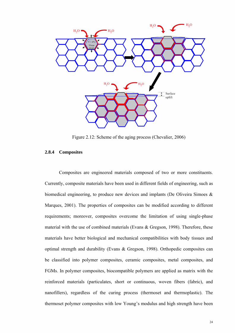
24
Figure 2.12: Scheme of the aging process (Chevalier, 2006)
2.8.4 Composites
Composites are engineered materials composed of two or more constituents.
Currently, composite materials have been used in different fields of engineering, such as
biomedical engineering, to produce new devices and implants (De Oliveira Simoes &
Marques, 2001). The properties of composites can be modified according to different
requirements; moreover, composites overcome the limitation of using single-phase
material with the use of combined materials (Evans & Gregson, 1998). Therefore, these
materials have better biological and mechanical compatibilities with body tissues and
optimal strength and durability (Evans & Gregson, 1998). Orthopedic composites can
be classified into polymer composites, ceramic composites, metal composites, and
FGMs. In polymer composites, biocompatible polymers are applied as matrix with the
reinforced materials (particulates, short or continuous, woven fibers (fabric), and
nanofillers), regardless of the curing process (thermoset and thermoplastic). The
thermoset polymer composites with low Young’s modulus and high strength have been

25
implemented in femoral prostheses and fixation devices (Scholz et al., 2011). However,
their performance in fixation devices is better than that in femoral prostheses (Evans &
Gregson, 1998). Moreover, thermoplastic polymer composites have been used in
acetabulum cups and artificial knee joint bearing.
Composite materials made of ceramics and metals are categorized based on the
matrix and reinforcing materials into ceramic–metal composites (CMCs) and metal–
ceramic composites (MCCs). The significant change in mechanical properties is caused
by the inclusion of ceramic or metal particles into the metal or ceramic matrixes
(Rodriguez-Suarez et al., 2012). Therefore, CMCs and MCCs possess superior stiffness,
fracture, fatigue, tribological, and thermal properties to their monolithic ceramic and
metal counterparts because of the overlapped strengths and weaknesses of the ceramics
and metals (Mattern et al., 2004). Accordingly, conventional and monolithic materials
(ceramics and metals) can rapidly change with these composites in various engineering
applications such as in aerospace and automobile industries (Sahin, 2005).
FGMs are special groups of composite materials that incorporate continuous
change (gradient) or step-wise change (graded) in their microstructure and properties as
shown in Figure 2.13 (Miao & Sun, 2009). This concept was obtained from their natural
biological structures (Pompe et al., 2003). Adapting materials with specific structural,
compositional, morphological, and mechanical properties have emphasized that FGMs
can be utilized in the design of new prostheses. The mechanical properties of FGMs can
be optimized and controlled by adjusting the volume fraction of each material phase
(Nie & Batra, 2010). In addition, the FGM-based implants provide better load bearing
capacity, fracture toughness, and wear resistance than their monolithic ceramic or
metallic counterparts (Miao & Sun, 2009; Mishina et al., 2008; Zhang et al., 2012).

26
Figure 2.13: A typical FGM structure: (a) gradient and (b) graded
2.9 Numerical methods in hip joint biomechanics and implant study
Numerical (computational) methods, such as finite element method (FEM),
extended FEM,and boundary element method, are powerful mathematical analysis tools
that are widely used in different fields of engineering. Numerical methods are well
accepted in biomedical engineering and biomechanics. In the numerical study of
implant design, various implant design configurations are considered in a computer
rather than performing expensive and destructive experimental tests (Asgari et al.,
2004). Accordingly, many researchers have used FEM in analyzing hip joint, hip joint
biomechanics, and hip implants. FEM has been used by prosthetists and engineers in the
hip implant design to address problems such as implant failure, stress shielding, and
bone resorption, which are related to the prosthesis material and design. The materials
for prosthesis were discussed by El-Sheikh et al. (2002), Akay and Aslan (1996),
Kaddick et al. (1997), Katoozian et al. (2001), Simões and Marques (2005), Kuiper and
Huiskes (1997), and Hedia et al. (2004; 2006). Moreover, El-Sheikh et al. (El-Sheikh et
al., 2002) examined the stress distribution in the implanted hip components to select the
optimal material for femoral prosthesis; the study was conducted by inserting a femoral
prosthesis with four different Young’s moduli: 25, 100, 196, and 400 GPa. The
(a) (b) (a) (b)

27
prostheses with lower Young’s modulus tolerate less stress compared with those with
higher Young’s modulus as shown in Figure 2.14. Moreover, the developed stresses
increase in the bone and cement.
Figure 2.14: Minimum and maximum principal stress distributions on the (a) lateral and (b) medial sides of the stem as a function of the prosthesis Young’s modulus (El-Sheikh et al., 2002)
Akay and Aslan (1996), Kaddick et al. (1997), Katoozian et al. (2001), and
Simões and Marques (2005) used FEM to determine whether composite materials can
replace the conventional materials used in femoral prosthesis. Katoozian et al. (2001)
investigated the effect of the fiber orientations in the composites on the stress
distribution in the implanted femur components. Moreover, Simões and Marques (2005)
used composite materials to construct a prosthesis with metal core and variable stiffness
as shown in Figure 2.15. High strain energy was observed in the proximal metaphysis of

28
the bone, indicating the less stress shielding effect of the prosthesis with tailorable
stiffness. However, more principal stress was detected in the bone because of the
implantation of the developed femoral prosthesis compared with those of the prostheses
composed of conventional materials.
Figure 2.15: A femoral prosthesis with metal core and variable stiffness (Simões & Marques, 2005)
Kuiper and Huiskes (1997) and Hedia et al. (2004; 2006) evaluated the FGM
performance in femoral prosthesis using two-dimensional (2D) FEM. The stress
shielding, interface stress, and developed stress in the implant decline when FGMs are
utilized in the femoral prosthesis. However, the developed stress in the bone and cement
increases. Moreover, designing and optimizing the geometry of a femoral prosthesis
using FEM were performed by Gross and Abel (2001), Sabatini and Goswami (2008),
Bennett and Goswami (2008), and Ramos et al. (2012). Gross and Abel used a hollow
stem to decrease prosthesis stiffness (rigidity) and stress shielding as shown in Figure
2.16.

29
Figure 2.16: Hollow stems introduced by Gross and Abel (Gross & Abel, 2001)
Sabatini and Goswami (2008) and Bennett and Goswami (2008) investigated the
effect of the different geometries of prostheses on stress distribution in the implanted
femur components. The different cross sections and profiles used in their studies are
presented in Figure 2.17.

30
Figure 2.17: Different cross-sections and profiles (Bennett & Goswami, 2008; Sabatini & Goswami, 2008)
Ramos et al. (2012) numerically examined various cemented femoral prostheses
with different cross sections and developed a new cemented femoral prosthesis
geometry as shown in Figure 2.18. The new design provides 25% less stress in the
cement compared with those of conventional prostheses.
Figure 2.18: Stem geometry developed by Ramos et al. (2012)

31
2.10 Load transfer in the proximal femur
All biological tissues have composite structures. This assumption is true for
bone–implant combinations. The bone and implant have different material properties.
Thus, an interface is required at which the two materials are integrated. One of the most
important issues in the bone-implant interfaces is the mechanism of transferring loads
from the implant to the surrounding bone. If the two materials are bonded and equal
forces are applied with equal strains, Hook’s law and some simple algebra should be
used to determine the load shared on each part of the composite structure as shown in
Equations (2.1) and (2.2).
i ii
i i b b
A E FF
A E A E
(2.1)
b bb
i i b b
A E FF
A E A E
(2.2)
where the subscript i denotes implant, and b represents the bone.
As indicated by these analogies for the composite structures and bone–implant
configurations, the load transfer mechanism in the femoral hip component exhibits
some basic characteristics, regardless of the stem shape and the precise joint load. These
basic characteristics can be illustrated by a simplified model of a straight implant
mounted on a straight bone tube (Figure 2.19) (Huiskes, 1988).
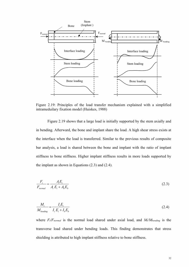
32
Figure 2.19: Principles of the load transfer mechanism explained with a simplified intrameduilary fixation model (Huiskes, 1988)
Figure 2.19 shows that a large load is initially supported by the stem axially and
in bending. Afterward, the bone and implant share the load. A high shear stress exists at
the interface when the load is transferred. Similar to the previous results of composite
bar analysis, a load is shared between the bone and implant with the ratio of implant
stiffness to bone stiffness. Higher implant stiffness results in more loads supported by
the implant as shown in Equations (2.3) and (2.4).
i i i
normal i i b b
F A E
F A E A E
(2.3)
i i i
bending i i b b
M I E
M I E I E
(2.4)
where Fi/Fnormal is the normal load shared under axial load, and Mi/Mbending is the
transverse load shared under bending loads. This finding demonstrates that stress
shielding is attributed to high implant stiffness relative to bone stiffness.

33
The mismatch between the bone and implant stiffness is important for
determining stress shielding and interface stress. Higher mismatches between the
implant and bone stiffness results in a higher degree of stress shielding because more
load is supported by the implant. However, as the implant carries more stress, lower
loads should be transferred to the bone, resulting in lower interface stress.
2.11 Bone
The skeleton is mostly composed of bony components. Unlike engineering
materials, bones are living tissues that can adapt to their mechanical and hormonal
environment. Bones are composite materials composed of minerals and collagen with
complex and unique mechanical properties. The bone functions are related to age,
disease, and use. Moreover, bones are considered FGMs with composition and property
dependent on direction and location. Long bones, such as femur, consist of two different
bony structures: spongy (cancellous or trabecular) and cortical (compact bone) (Figure
2.20).
Figure 2.20: Bone structure (Juillard, 2011)
34
2.12 Summary
This chapter presented a brief review regarding the hip joint and THR. Several
studies have been performed to determine the optimal material and geometrical design
for femoral prosthesis. However, an optimal hip design remains ambiguous and should
be further investigated. Previous studies have focused only on the materials or
geometrical design for prosthesis. The increasing incidence of THR involving young
patients has motivated the use of FGMs in femoral prosthesis to prolong the lifespan of
THR.

35
CHAPTER 3
3. MATERIALS AND METHODS
3.1 Introduction
This chapter describes the methods performed in the current study. This chapter
also presents the strategies developed to serve as guidelines throughout the study and
aid in achieving the desired objectives.
3.2 Outline of Methodology
An outline of methodology is presented using a flow chart in Figure 3.1. The
outline provides an overview of the whole process and followed by a detailed discussion
regarding the procedures and techniques used for FEA and experiment. The main
activities in this study include FEA and experimental tests, which are described in this
section.
3.3 Finite element analysis
3.3.1 Finite element modeling to use functionally graded materials in femoral prosthesis
A general finite element model was used to evaluate the performance of
functionally graded (FG) femoral prostheses. Figure 3.2 presents an FEA flow chart.
ABAQUS (ABAQUS Inc., Providence, RI, USA) version 6.10, a finite element
software package, was used to determine the performance of FG femoral prostheses.

36
Figure 3.1: General description of the methodology adopted in the study

37
Figure 3.2: General description of the finite element analysis adopted in the study

38
3.3.2 Bone modeling
Computed tomography (CT) images were used to extract three-dimensional (3D)
models of an anatomical femur. The properties of the CT scan slices are presented in
Table 3.1.
Table 3.1: CT scan slices
Materials Properties Width 512 pixels Height 512 pixels Pixel size 0.549 mm Algorithm B10s Reduction 1 Field of view 28.10 cm Gantry tilt 0.000° Number of slices 988 Slice increment 0.699 mm
The images were captured using a multidetector Siemens unit (Sensation 64; Siemens
Medical Solutions, Malvern, PA, USA). The CT images were converted into the Digital
Imaging and Communication (DICOM) format and imported to the Mimic® software
(version 13; Materialise NV, Leuven, Belgium). The femur was identified using tissue-
specific threshold values of 148 HU – 1,872 HU (the maximum and minimum threshold
values corresponded to the range of grey values to the highlighted pixels). The
simplified model of the femur also developed with Solidworks (Solidworks 2012,
Dassault Systèmes Solidworks Corp., USA) computer-aided design software. The 3D
anatomical model of the femur was developed using Mimic® software (Figure 3.3a),
whereas the simplified model was constructed using Solidworks (Figure 3.3b).

39
Figure 3.2: Development of the three-dimensional model of the femur using Mimic® software
Figure 3.3: Three-dimensional models of the femur: (a) anatomical and (b) simplified
(a) (b)

40
3.3.3 Prosthesis modeling
Solidworks (Solidworks 2012, Dassault Systèmes Solidworks Corp., USA) was
used to develop a 3D model of the femoral prosthesis. Some of the 3D models of
femoral prostheses are presented in Figure 3.4. The models for femoral prostheses with
different geometries were developed using Solidworks. The prostheses composed of
five distal cross sections, four proximal cross sections, and three profiles (Figure 3.5).
Figure 3.4: Stem models developed using Solidworks

41
(a)
Profile 1 Profile 2 Profile 3
(b)
P1 P2 P3 P4
(c)
D1 D2 D3 D4 D5
Figure 3.5: Dimensions of (a) profile, (b) proximal cross-sections, and (c) distal cross-sections

42
3.3.4 Mesh generation
The 3D tetrahedral elements were used to mesh the implanted femur constituents
(Ramos & Simoes, 2006). The approximate global sizes to mesh the cement, femoral
prosthesis, and femur are 2, 1.5, and 2 mm, respectively.
3.3.5 Boundary conditions
A range of loading conditions from the hip contact force to more complex
loading scenarios involving several muscle forces can be used to represent the hip
loading conditions. Moreover, two scenarios should be considered at the bone–implant
surface for cementless prosthesis implantation. These conditions include non-bonded
with friction coefficient and bonded surfaces. The non-bonded condition represents the
prior bone in-growth, whereas the bonded surfaces depict the ideal bone in-growth. The
desired fixation in cementless prostheses does not immediately occur after surgery.
Moreover, the primary stability of a prosthesis can be evaluated by modeling the
prosthesis and the straight bone after surgery. In this study, two conditions were
considered on the bone–implant surface, namely, non-bonded surfaces with coefficients
of friction of 0.4 and bonded surfaces. Friction Coefficients of 0.4 was also considered
between the prosthesis and cement.
3.3.6 Material properties
The materials considered in this study for femoral prosthesis are included
conventional material (Titanium alloy, Stainless steel and chrome cobalt) and
functionally graded material (Titanium alloy-HA and Stainless steel-HA). Ti alloy, St,
Cr–Co, and HA are linear isotropic elastic materials. The cortical bone is a transversely
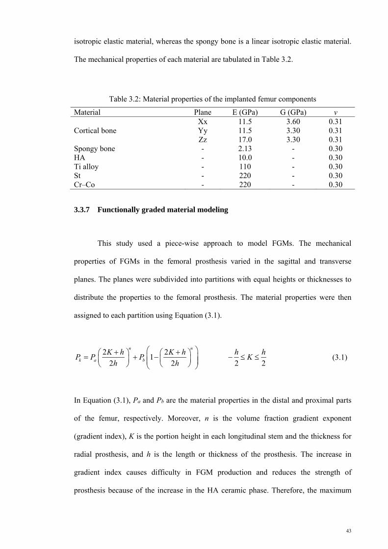
43
isotropic elastic material, whereas the spongy bone is a linear isotropic elastic material.
The mechanical properties of each material are tabulated in Table 3.2.
Table 3.2: Material properties of the implanted femur components
Material Plane E (GPa) G (GPa) v
Cortical bone Xx 11.5 3.60 0.31 Yy 11.5 3.30 0.31 Zz 17.0 3.30 0.31
Spongy bone - 2.13 - 0.30 HA - 10.0 - 0.30 Ti alloy - 110 - 0.30 St - 220 - 0.30 Cr–Co - 220 - 0.30
3.3.7 Functionally graded material modeling
This study used a piece-wise approach to model FGMs. The mechanical
properties of FGMs in the femoral prosthesis varied in the sagittal and transverse
planes. The planes were subdivided into partitions with equal heights or thicknesses to
distribute the properties to the femoral prosthesis. The material properties were then
assigned to each partition using Equation (3.1).
2 21
2 2 2 2
n n
k a b
K h K h h hP P P K
h h
(3.1)
In Equation (3.1), Pa and Pb are the material properties in the distal and proximal parts
of the femur, respectively. Moreover, n is the volume fraction gradient exponent
(gradient index), K is the portion height in each longitudinal stem and the thickness for
radial prosthesis, and h is the length or thickness of the prosthesis. The increase in
gradient index causes difficulty in FGM production and reduces the strength of
prosthesis because of the increase in the HA ceramic phase. Therefore, the maximum
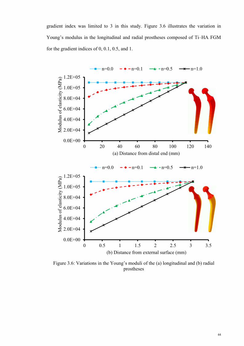
44
gradient index was limited to 3 in this study. Figure 3.6 illustrates the variation in
Young’s modulus in the longitudinal and radial prostheses composed of Ti–HA FGM
for the gradient indices of 0, 0.1, 0.5, and 1.
Figure 3.6: Variations in the Young’s moduli of the (a) longitudinal and (b) radial prostheses
0.0E+00
2.0E+04
4.0E+04
6.0E+04
8.0E+04
1.0E+05
1.2E+05
0 20 40 60 80 100 120 140
Mod
ulus
of
elas
tici
ty (
MP
a)
(a) Distance from distal end (mm)
n=0.0 n=0.1 n=0.5 n=1.0
0.0E+00
2.0E+04
4.0E+04
6.0E+04
8.0E+04
1.0E+05
1.2E+05
0 0.5 1 1.5 2 2.5 3 3.5
Mod
ulus
of
elas
tici
ty (
MP
a)
(b) Distance from external surface (mm)
n=0.0 n=0.1 n=0.5 n=1.0

45
3.3.8 Crack modeling
Three different conditions were considered to assess the crack behavior inside the
cement layer. These conditions include the location of cracks along the cement layer,
position of cracks on the internal or external surface of the cement layer, and interaction
of cracks on each other. The cement layer suffers from normal and shearing stresses,
which are applied at the cement layer in hoop and longitudinal directions. Accordingly,
the circumferential crack may propagate in the cement layer at different positions. The
crack sizes range from micro to macro. In this study, the depths of the internal and
external circumferential cracks were assumed to be 0.5 mm within the cement layer of
THR. Moreover, the location of the cracks on the internal and external surfaces of the
cement layer along the cement length was modified to reveal the places with higher risk
of fracture and crack growth rate. Moreover, damage tolerance was based on the
likelihood of finding cracks and their estimated propagation rates. Then, the cracks were
positioned in the cement with the following distances: 25 (internal crack, I25; external
crack, E25), 50 (internal crack, I50; external crack, E50), 75 (internal crack, I75; external
crack, E75), and 100 mm (internal crack, I100; external crack, E100) from the distal end.
The models tabulated in Table 1 included the length of the cement with an equidistance
of 25 mm from the distal end to the proximal end on its internal and external surfaces.
The models also present the relationship between the distance from the distal end and
the behavior of stress intensity factor (SIF). An example of an internal crack at different
locations is presented in Figure 3.7.

46
Figure 3.7: Internal crack geometry and locations of crack in the cement layer at (a) 25, (b) 50, (c) 75, and (d) 100 mm
3.3.9 Validation of finite element models
After several executions of the model, the errors in the mesh, material model,
and boundary conditions were corrected, and the general finite element model was
validated. The validation process involved the analysis of the convergence and
investigation of the model under various conditions. The convergence of the results was
the criterion used for validation. When errors were found during the validation process,
a secondary literature survey was conducted to obtain pertinent insights from other
studies.

47
3.4 Experimental procedure
Figure 3.8 shows the experimental steps performed in the present study.
Figure 3.8: Flowchart of the experimental procedure
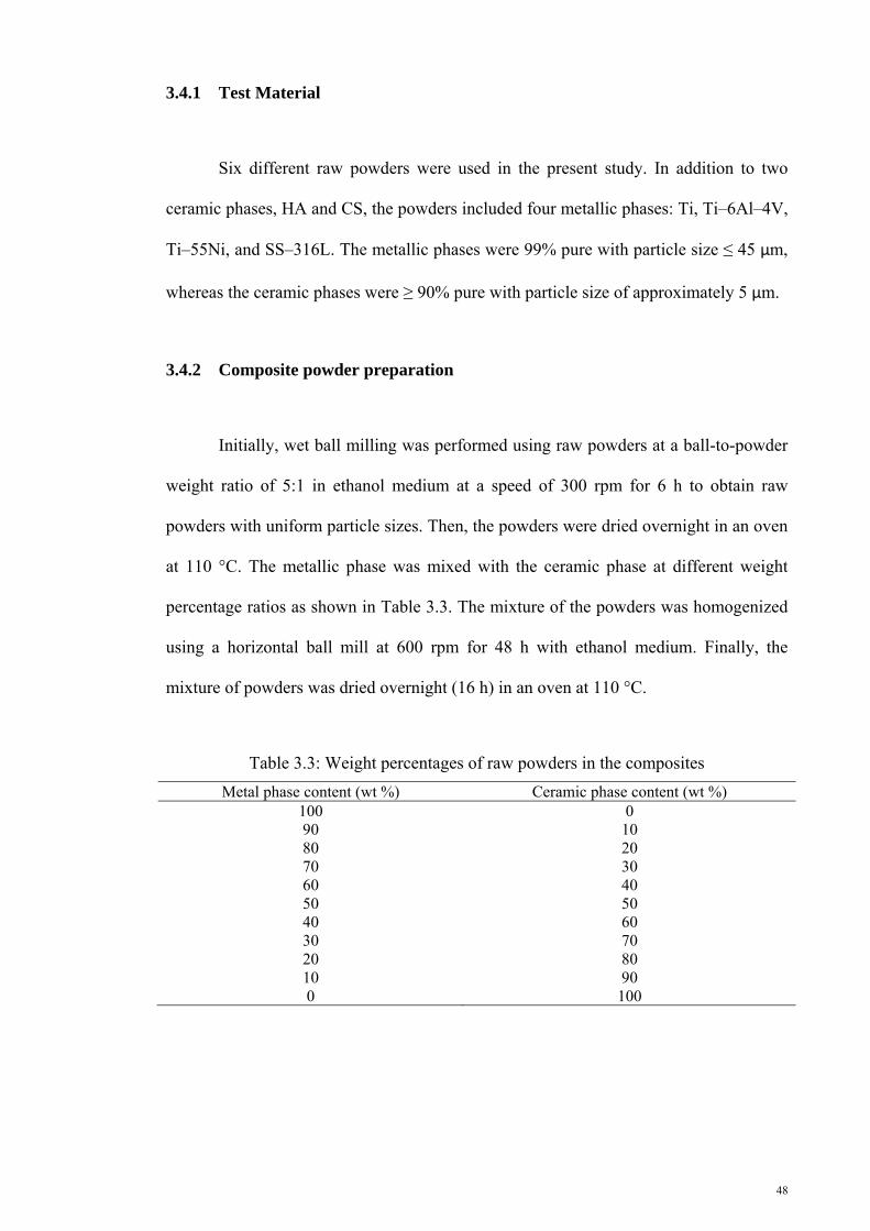
48
3.4.1 Test Material
Six different raw powders were used in the present study. In addition to two
ceramic phases, HA and CS, the powders included four metallic phases: Ti, Ti–6Al–4V,
Ti–55Ni, and SS–316L. The metallic phases were 99% pure with particle size ≤ 45 µm,
whereas the ceramic phases were ≥ 90% pure with particle size of approximately 5 μm.
3.4.2 Composite powder preparation
Initially, wet ball milling was performed using raw powders at a ball-to-powder
weight ratio of 5:1 in ethanol medium at a speed of 300 rpm for 6 h to obtain raw
powders with uniform particle sizes. Then, the powders were dried overnight in an oven
at 110 °C. The metallic phase was mixed with the ceramic phase at different weight
percentage ratios as shown in Table 3.3. The mixture of the powders was homogenized
using a horizontal ball mill at 600 rpm for 48 h with ethanol medium. Finally, the
mixture of powders was dried overnight (16 h) in an oven at 110 °C.
Table 3.3: Weight percentages of raw powders in the composites
Metal phase content (wt %) Ceramic phase content (wt %) 100 0 90 10 80 20 70 30 60 40 50 50 40 60 30 70 20 80 10 90 0 100

49
3.4.3 Test specimen preparation
The dried milled powders were compacted at 250 MPa using a manual
hydraulic press (GS15011, Graseby Specac) to form green samples. Afterwards,
pressureless sintering was performed at 1,200 °C for the composite sample and at
1,200 °C, 1,100 °C, and 1,000 °C for the FGM samples for 3 h in an inert argon gas
environment using a vacuum atmosphere furnace (XY1600, Nanyang Xinyu Furnaces).
Sintering was conducted to prevent the oxidation of the metal phases. The entire test
procedure was performed on each specimen. The specimens were prepared in a
cylindrical form with diameter of 6.35 mm and length of 12.7 mm according to the
ASTM C 773-8 (Figure 3.9).
Figure 3.9: Typical testing of sample
3.4.4 Structure characterization
X-ray diffraction (XRD) was conducted on the sintered samples using an X-ray
diffractometer (Empyrean, PANalytical) to determine and analyze the phase
constitution. Scanning angle (2θ) ranged from 20° to 70° using CuKα radiation (λ =
1.54056 Å).
50
3.4.5 Physical characterization
Density (ρ, g/cc) was measured using Archimedes’ principle as discussed in a
previous study (Pramanik et al., 2012) and is presented by Equation (3.2), whereas the
volume shrinkage (%) of the sintered samples was determined with Equation (3.3). A
minimum of five identical specimens were obtained. The average and standard
deviation (STD) for each sintered sample were determined using the water density of
0.99704 g/mL at 25 °C.
in air
in air in water
WeightDensity Water density
Weight Weight
(3.2)
% 100Initial volume Final volume
Volume Shrinkage percentageInitial volume
ò e (3.3)
3.4.6 Mechanical characterization
3.4.6.1 Vickers hardness test
Vickers hardness test was conducted on the polished surfaces of the sintered
samples using a microVicker’s hardness tester (Figure 3.10; AVK-C200, Mitutoyo).
The pyramid-shaped diamond indenter was used at a constant load of 5 N for 10 s to
obtain a minimum of five indentations from each sample.

51
Figure 3.10: A micro-hardness tester machine
3.4.6.2 Compressive static test
The specimens were subjected to compressive static test at room temperature to
determine the compressive elastic modulus ( CE ) and ultimate compressive strength
(σUCS) of the composites. The test was conducted using a universal testing machine as
presented in Figure 3.11 (4469, Instron). The test was performed under load control
condition at a displacement rate of constant cross-head speed of 1 mm/min.
Figure 3.11: An Instron universal testing machine

52
3.5 Summary
This chapter described the overview of the methodology used in this study to
achieve the desired objectives. The methodology was divided into two parts: finite
element modeling and experimentation. Finite element method included the modeling of
longitudinal, radial, and longitudinal–radial Charnley FG femoral prostheses as well as
the longitudinal and radial FG femoral prostheses with different geometries. Moreover,
the experiments included the preparation of the composites of Ti, Ti–Ni, Ti–6Al–4V,
and SS–316L with CS and HA to assess their composition structure and compressive
properties as a function of the ceramic phase weight percentage after sintering at
1,200 °C. In addition, FGMs composed of Ti, Ti–Ni, Ti–6Al–4V, and SS–316L with CS
and HA were prepared. The FGMs sintered at 1000 °C, 1100 °C, and 1200 °C and their
physical and compressive mechanical properties were also assessed.

53
CHAPTER 4
4. RESULTS
4.1 Introduction
This chapter is divided into two parts: FEA and experimental results. The FEA
results obtained using the models are divided into four parts: longitudinal, radial, and
longitudinal–radial FG Charnley femoral prosthesis, cementless FG prostheses,
cemented FG prostheses, and cemented prostheses with circumferential cracks. The
SED at the proximal of the femur was determined to examine the stress shielding level
of the prosthesis. The risk of failure of prostheses was examined by assessing the
developed von Mises stress. The maximum and minimum principal stresses stimulated
to the bone were used as failure criterion. Cement failure was investigated by measuring
the maximum and minimum principal stresses induced to the cement. The induced shear
interface stresses were used to obtain the risk of failure in the interfaces.
Circumferential crack behavior was studied by investigating SIFs, namely, KI, KII, and
KIII, at the crack front. The experimental results are divided into two parts: metal (Ti,
Ti–6Al–4V, Ti–55Ni, and SS-316L)–ceramic (CS and HA) composites and FGMs. The
experimental results include physical properties, XRD, static compression, and Vickers
hardness. Physical properties include shrinkage and density. The experimental results
for compressive static test at ambient temperature provide the material properties,
including compressive Young’s modulus, ultimate compressive strength, and strain
percentage at the maximum load.
54
4.2 Finite element analysis
This section presents the results of FEA using the implanted femur with
different configurations (Figure 4.1). The FEA results were obtained by implanting
cementless and cemented FG Charnley femoral prostheses in the anatomical model of
the femur. The results of implanting the cementless prostheses with different geometries
composed of conventional materials and FGMs were also presented. Moreover, the
results of inserting the cemented prostheses made of conventional materials and FGMs
with different geometries in the anatomical femur were demonstrated. The results of the
presence of the circumferential cracks in the cement layer were discussed at the end of
this section.

55
Figure 4.1: Flow chart of result presentation
56
4.2.1 Longitudinal, radial, and longitudinal–radial FG Charnley femoral prostheses
The changes in the Young’s modulus of the longitudinal, radial, and
longitudinal–radial Charnley femoral prostheses were investigated. In the FG
longitudinal femoral prostheses (LP), the Young’s modulus gradually increased from
the distal to the proximal direction in the sagittal plane as shown in Figure 3.8a.
Moreover, the Young’s modulus of the FG radial femoral prostheses (RP) was altered in
the transverse plane and gradually increased in the direction of the cortex layers to the
core of the prostheses (Figure 3.8b). For the longitudinal–radial prostheses (L-RP), the
Young’s modulus was simultaneously altered in the sagital and transverse planes. Thus,
the stiffness of the prostheses from distal to proximal and from the cortex layer to the
core simultaneously increased.
4.2.1.1 Strain energy density
Figure 4.2 shows the variation in the SED in the proximal metaphysis of the
femur implanted with different FG femoral prostheses. SED is illustrated in four
different bar charts according to the action models (normal walking and stair climbing)
and the fixation methods of the prostheses inside the bone (cemented and non-
cemented). The horizontal and vertical axes in the bar charts depict the variation in the
gradient index in the longitudinal direction and SED (J/mm3), respectively. The legend
indicates the changes in the gradient indices in the radial direction. SED exhibited an
increasing trend with the longitudinal and radial gradient index, regardless of the action
and fixation method. As indicated in each graph, the prostheses with longitudinal and
radial gradient indices equal to 0 showed the lowest SED in the bone, whereas those
equal to 1 demonstrated the highest SED. The SED minimum values of 282.8 (cemented
prosthesis, normal walking), 288.0 (cementless prosthesis, normal walking), 303.1

57
(cemented prosthesis, stair climbing), and 304.1 J/mm3 (cementless prosthesis, stair
climbing) increased to the maximum values of 409.7, 543.1, 434.0, and 545.3 J/mm3,
respectively, when the gradient index increased from 0 to 1. This finding was consistent
with the adverse relatioship between prosthesis stiffness and induced SED to the bone.
Composite beam theory and Equations (2.1) to (2.3) indicate that more loads are
induced to the other components of THR when the prosthesis stiffness decreases. Thus,
higher SED is developed in the bone. The effect of the increase in the radial gradient
index on SED was higher than that of the longitudinal gradient index. For example, in
cementless prosthesis during normal walking, when the radial gradient index (n) was 0
and the longitudinal gradient index (m) increased from 0 to 1, SED increased from
288.0 J/mm3 to 360.3 J/mm3. However, when m = 0 and n increased from 0 to 1, SED
increased from 288.0 J/mm3 to 465.4 J/mm3. In the cemented prosthesis, a portion of
load was carried and damped by the cement. Therefore, lower loads were transferred to
the bone. Thus, the cementless FG prostheses produced 11.8% higher SED than the
cemented prosthesis during normal walking and stair climbing. Moreover, normal
walking provided lower loads to the components of the artificial hip joints.
Accordingly, the SED in the femur was lower during normal walking [409.7 (cemented
prosthesis) and 543.1 J/mm3 (cementless prosthesis)] than that during stair climbing
[434.0 (cemented prosthesis) and 545.3 J/mm3 (cementless prosthesis)].

58
n is the radial gradient index
n is the radial gradient index
0
100
200
300
400
500
600
m=0.0 m=0.1 m=0.5 m=1.0
Str
ain
ener
gy d
ensi
ty (
J/m
m3 )
(a) Longitudinal gradient index
n=0.0 n=0.1 n=0.5 n=1.0
0
100
200
300
400
500
600
m=0.0 m=0.1 m=0.5 m=1.0
Str
ain
ener
gy d
ensi
ty (
J/m
m3 )
(b) Longitudinal gradient index
n=0.0 n=0.1 n=0.5 n=1.0

59
n is the radial gradient index
n is the radial gradient index
Figure 4.2: Strain energies in the spongy portion of the proximal metaphysis of the femur caused by implantation of (a) normal walking–cemented, (b) normal walking–non-cemented, (c) stair climbing–cemented, and (d) stair climbing–non-cemented prostheses. (The legend shows the changes in the radial volume fraction gradient exponent)
0
100
200
300
400
500
600
m=0.0 m=0.1 m=0.5 m=1.0
Str
ain
ener
gy d
ensi
ty (
J/m
m3 )
(c) Longitudinal gradient index
n=0.0 n=0.1 n=0.5 n=1.0
0
100
200
300
400
500
600
m=0.0 m=0.1 m=0.5 m=1.0
Str
ain
ener
gy d
ensi
ty (
J/m
m3 )
(d) Longitudinal gradient index
n=0.0 n=0.1 n=0.5 n=1.0
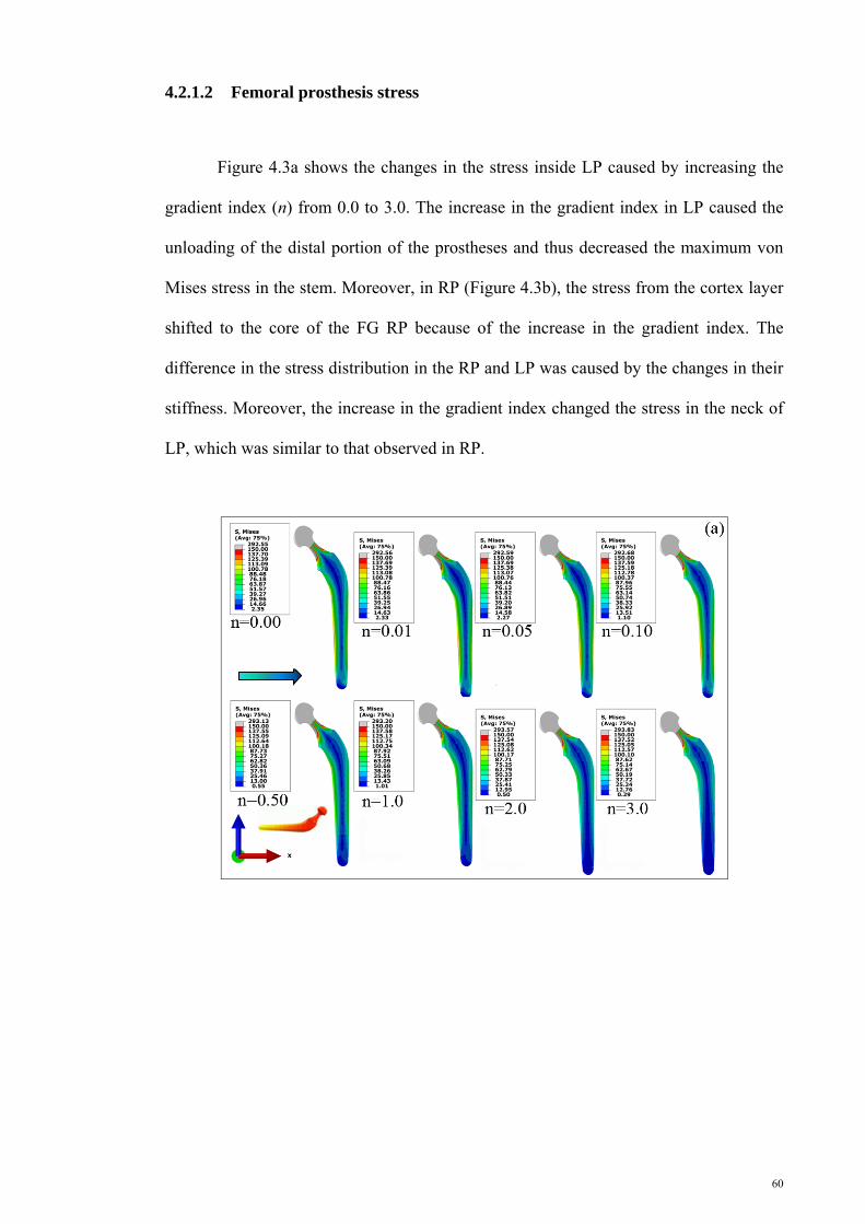
60
4.2.1.2 Femoral prosthesis stress
Figure 4.3a shows the changes in the stress inside LP caused by increasing the
gradient index (n) from 0.0 to 3.0. The increase in the gradient index in LP caused the
unloading of the distal portion of the prostheses and thus decreased the maximum von
Mises stress in the stem. Moreover, in RP (Figure 4.3b), the stress from the cortex layer
shifted to the core of the FG RP because of the increase in the gradient index. The
difference in the stress distribution in the RP and LP was caused by the changes in their
stiffness. Moreover, the increase in the gradient index changed the stress in the neck of
LP, which was similar to that observed in RP.

61
Figure 4.3: Variation in the von Mises stress in the prosthesis as a function of volume fraction gradient exponent in the non-cemented (a) longitudinal and (b) radial prostheses
Figure 4.4: Stress variations in the longitudinal femoral prosthesis during normal walking at the (a) lateral and (b) medial sides of cemented prosthesis as well as at the (c) lateral and (d) medial sides of the cementless prosthesis
(d)
(b)
von
Mis
es s
tres
s (M
Pa)
Femoral prosthesis length (mm)
(n) enhancement
Femoral prosthesis length (mm)
(c)
(a)

62
Figure 4.5: Stress variation in the longitudinal femoral prosthesis in stair climbing at the (a) lateral and (b) medial sides of the cemented prosthesis as well as at the (c) lateral and (d) medial sides of the cementless prosthesis
Figures 4.4 and 4.5 depict the stress variation at the lateral and medial sides of
LP as a function of the prosthesis length. The stress variation during normal walking
and stair climbing showed a similar trend with the increasing prosthesis length. Concave
plots for different gradient indices were observed, whereas the peak value of the stress
decreased with the increase in the gradient index. For example, in the longitudinal
cemented prosthesis under normal walking, the peak stress decreased from 48.9 MPa to
39.1 MPa at the lateral side and from 53.2 MPa to 43.6 MPa at the medial side. The
cementless longitudinal prosthesis also showed decreased peak stresses from 47.0 MPa
to 38.6 MPa (at lateral side) and from 61.1 MPa to 52.3 MPa (at medial side). The
femoral prosthesis was under bending loading, and more loads were transferred at the
medial side. Therefore, the medial side of the cemented and cementless femoral
prostheses exhibited about 21.4% more stress than the lateral side of the femur. The
peak values of the von Mises stress on the prostheses with different material models are
(c) (d)
(b) (a)
von
Mis
es s
tres
s (M
Pa)
Femoral prosthesis length (mm)

63
presented in Table 4.1. Similar to Figures 4.4 and 4.5, the stress decreased as the
gradient index increased because of the reduced stiffness of the prostheses and the
higher loads shared between the prostheses and the other components of THR.
Accordingly, during normal walking and stair climbing, the cemented and cementless
prostheses with 0 longitudinal and radial gradient indices exhibited the highest values
for stress: 53.2 (cemented prosthesis, normal walking), 76.7 (cemented prosthesis, stair
climbing), 61.1 (cementless prosthesis, normal walking), and 60.6 MPa (cementless
prosthesis, stair climbing). However, the prostheses with radial and longitudinal
gradient indices equal to 1 demonstrated the lowest values for stress: 12.1 (cemented
prosthesis, normal walking), 13.7 (cemented prosthesis, stair climbing), 16.8
(cementless prosthesis, normal walking), and 16.1 MPa (cementless prosthesis, stair
climbing). The cementless prostheses tolerated about 13.8% lower stress than the
cemented prostheses under normal walking and stair climbing (Table 4.1).
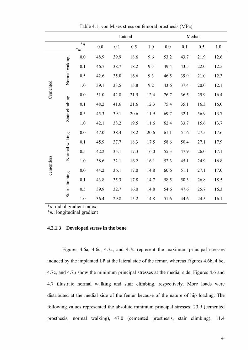
64
Table 4.1: von Mises stress on femoral prosthesis (MPa)
Lateral Medial
*n *m
0.0 0.1 0.5 1.0 0.0 0.1 0.5 1.0 C
emen
ted Nor
mal
wak
ing 0.0 48.9 39.9 18.6 9.6 53.2 43.7 21.9 12.6
0.1 46.7 38.7 18.2 9.5 49.4 43.5 22.0 12.5
0.5 42.6 35.0 16.6 9.3 46.5 39.9 21.0 12.3
1.0 39.1 33.5 15.8 9.2 43.6 37.4 20.0 12.1
Sta
ir c
lim
bing
0.0 51.0 42.8 21.5 12.4 76.7 36.5 29.9 16.4
0.1 48.2 41.6 21.6 12.3 75.4 35.1 16.3 16.0
0.5 45.3 39.1 20.6 11.9 69.7 32.1 56.9 13.7
1.0 42.1 38.2 19.5 11.6 62.4 33.7 15.6 13.7
cem
entl
ess
Nor
mal
wak
ing 0.0 47.0 38.4 18.2 20.6 61.1 51.6 27.5 17.6
0.1 45.9 37.7 18.3 17.5 58.6 50.4 27.1 17.9
0.5 42.2 35.1 17.3 16.0 55.3 47.9 26.0 17.1
1.0 38.6 32.1 16.2 16.1 52.3 45.1 24.9 16.8
Sta
ir c
lim
bing
0.0 44.2 36.1 17.0 14.8 60.6 51.1 27.1 17.0
0.1 43.8 35.3 17.8 14.7 58.5 50.3 26.8 18.5
0.5 39.9 32.7 16.0 14.8 54.6 47.6 25.7 16.3
1.0 36.4 29.8 15.2 14.8 51.6 44.6 24.5 16.1
*n: radial gradient index *m: longitudinal gradient
4.2.1.3 Developed stress in the bone
Figures 4.6a, 4.6c, 4.7a, and 4.7c represent the maximum principal stresses
induced by the implanted LP at the lateral side of the femur, whereas Figures 4.6b, 4.6e,
4.7c, and 4.7b show the minimum principal stresses at the medial side. Figures 4.6 and
4.7 illustrate normal walking and stair climbing, respectively. More loads were
distributed at the medial side of the femur because of the nature of hip loading. The
following values represented the absolute minimum principal stresses: 23.9 (cemented
prosthesis, normal walking), 47.0 (cemented prosthesis, stair climbing), 11.4

65
(cementless prosthesis, normal walking), and 23.3 MPa (cementless prosthesis, stair
climbing) at the medial side. These values were higher than their corresponding
absolute maximum principal stresses: 17.9, 20.8, 10.9, and 11.2 MPa at the lateral side
of the femur. The increase in the gradient index affected the stress variation at the lateral
and medial sides of the femur, whereas the stress increased because more loads were
distributed as a result of the reduced stiffness.
Figure 4.6: Stress variation in the femur during normal walking. (a) Maximum principal stress and cemented prosthesis, (b) minimum principal stress and cemented prosthesis, (c) maximum principal stress and cementless prosthesis, and (d) minimum principal stress and cementless prosthesis
(c) (d)
(b) (a)
Max
imum
and
min
imum
pri
ncip
al s
tres
s (M
Pa)
Femoral prosthesis length (mm)
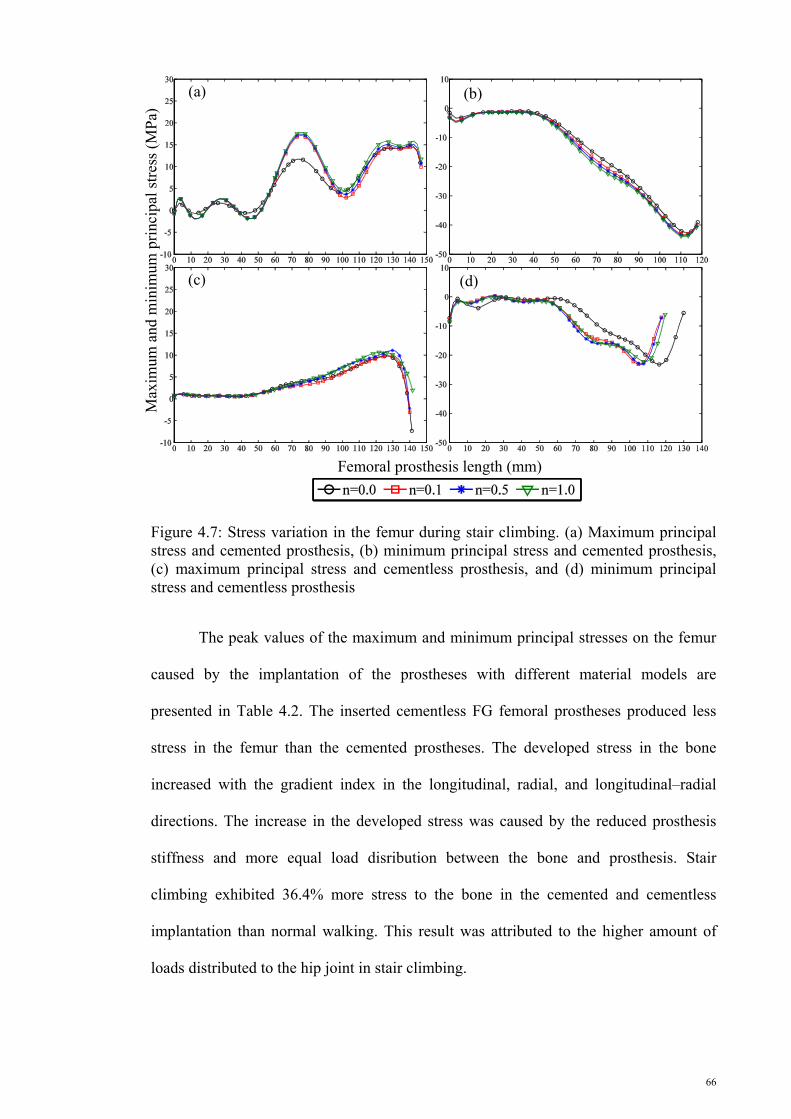
66
Figure 4.7: Stress variation in the femur during stair climbing. (a) Maximum principal stress and cemented prosthesis, (b) minimum principal stress and cemented prosthesis, (c) maximum principal stress and cementless prosthesis, and (d) minimum principal stress and cementless prosthesis
The peak values of the maximum and minimum principal stresses on the femur
caused by the implantation of the prostheses with different material models are
presented in Table 4.2. The inserted cementless FG femoral prostheses produced less
stress in the femur than the cemented prostheses. The developed stress in the bone
increased with the gradient index in the longitudinal, radial, and longitudinal–radial
directions. The increase in the developed stress was caused by the reduced prosthesis
stiffness and more equal load disribution between the bone and prosthesis. Stair
climbing exhibited 36.4% more stress to the bone in the cemented and cementless
implantation than normal walking. This result was attributed to the higher amount of
loads distributed to the hip joint in stair climbing.
(c)
Max
imum
and
min
imum
pri
ncip
al s
tres
s (M
Pa)
Femoral prosthesis length (mm)
(a) (b)
(d)

67
Table 4.2: Maximum and minimum principal stresses on the femur (MPa).
Maximum principal stress Minimum principal stress
Lateral Medial
*n *m
0.0 0.1 0.5 1.0 0.0 0.1 0.5 1.0
Cem
ente
d Nor
mal
wak
ing 0.0 16.4 16.8 18.0 18.9 23.4 24.5 24.4 24.6
0.1 16.6 17.0 18.2 19.1 23.4 24.7 25.0 25.2
0.5 17.2 17.5 18.7 19.5 23.6 25.0 25.2 25.4
1.0 17.9 18.8 19.3 19.9 23.9 25.0 25.5 25.6
Sta
ir c
lim
bing
0.0 19.5 19.9 21.2 22.1 46.7 46.7 46.5 46.7
0.1 19.7 20.1 21.3 22.2 46.4 47.0 47.4 47.7
0.5 20.2 20.6 21.7 22.6 46.7 47.5 47.8 48.0
1.0 20.8 21.3 22.2 23.0 47.0 67.5 48.1 48.2
Cem
entl
ess
Nor
mal
wak
ing 0.0 10.2 10.3 10.6 10.8 9.8 10.0 10.8 13.6
0.1 10.4 10.4 10.5 10.6 10.9 13.9 14.5 14.9
0.5 11.0 10.5 10.5 10.6 11.0 15.5 15.5 15.3
1.0 10.9 10.6 10.7 10.7 11.4 15.9 15.5 15.4
Sta
ir c
lim
bing
0.0 10.0 10.1 10.6 10.9 25.0 25.0 25.1 25.1
0.1 10.5 10.6 10.8 11.0 24.1 24.5 24.7 24.7
0.5 11.5 10.9 11.0 11.0 23.8 24.1 24.4 24.6
1.0 11.2 10.9 10.9 10.9 23.3 24.0 24.3 24.7
*n: radial gradient index *m: longitudinal gradient
4.2.1.4 Developed stress in the cement
The maximum principal stress variations on the internal and external surfaces of
the cement layer induced by the implantation of LP during normal walking and stair
climbing are presented in Figure 4.8. The peak values of stresses were observed at the
distal and proximal end along the middle length of the cement layer. The peak values of
the stresses on the internal and external surfaces of the cement layer increased along
with gradient index during normal walking and stair climbing. The highest value of

68
stress in the cement layer was induced by the FG prosthesis with a gradient index of 1.0,
whereas the prosthesis with gradient index of 0.0 provided the minimum stress in the
cement layer.
Figure 4.8: Stress variation in the cement layers during normal walking [(a) internal and (b) external layers] and stair climbing [(c) internal and (d) external layers]
Figure 4.9 displays the maximum principal stress variation on the external and
the internal surfaces of the cement layer caused by implanting RP. The maximum
principal stress showed similar trend along the cement length in both surfaces (internal
and external surfaces) and both action models (normal walking and stair climbing). The
maximum principal stress behavior in the cement was similar to the behavior induced
by inserting LP.
(c)
Max
imum
pri
ncip
al s
tres
s (M
Pa)
Femoral prosthesis length (mm)
(a) (b)
(d)

69
Figure 4.9: Stress variation in the cement layers during normal walking [(a) internal and external layers] and stair climbing [(c) internal and (d) external layers]
The maximum principal stresses computed on the internal and external surfaces
of the cement and the peak values of the maximum principal stress calculated based on
the different gradient indexes of the prostheses are presented in Table 4.3. Similar to the
response of stress to the increase in the gradient index on the bone, the stress on the
internal and external surfaces of the cement increased with the gradient index (Table
4.3). On the external surface of the cement layer, the stress during stair climbing was
22.3% higher than that during normal walking. However, the internal surface of the
cement layer had 27.8% more stress during normal walking than that during stair
climbing.
(c)
Max
imum
pri
ncip
al s
tres
s (M
Pa)
Femoral prosthesis length (mm)
(a) (b)
(d)
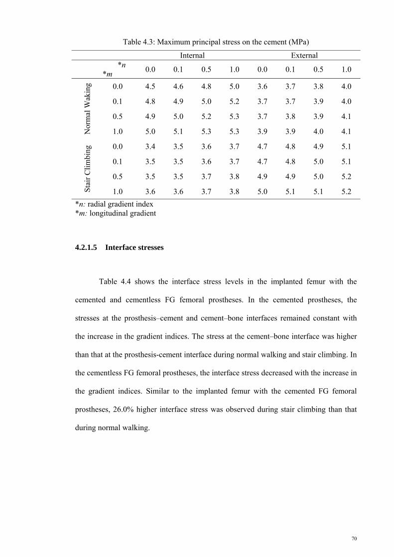
70
Table 4.3: Maximum principal stress on the cement (MPa)
Internal External
*n
*m 0.0 0.1 0.5 1.0 0.0 0.1 0.5 1.0
Nor
mal
Wak
ing 0.0 4.5 4.6 4.8 5.0 3.6 3.7 3.8 4.0
0.1 4.8 4.9 5.0 5.2 3.7 3.7 3.9 4.0
0.5 4.9 5.0 5.2 5.3 3.7 3.8 3.9 4.1
1.0 5.0 5.1 5.3 5.3 3.9 3.9 4.0 4.1
Sta
ir C
lim
bing
0.0 3.4 3.5 3.6 3.7 4.7 4.8 4.9 5.1
0.1 3.5 3.5 3.6 3.7 4.7 4.8 5.0 5.1
0.5 3.5 3.5 3.7 3.8 4.9 4.9 5.0 5.2
1.0 3.6 3.6 3.7 3.8 5.0 5.1 5.1 5.2
*n: radial gradient index *m: longitudinal gradient
4.2.1.5 Interface stresses
Table 4.4 shows the interface stress levels in the implanted femur with the
cemented and cementless FG femoral prostheses. In the cemented prostheses, the
stresses at the prosthesis–cement and cement–bone interfaces remained constant with
the increase in the gradient indices. The stress at the cement–bone interface was higher
than that at the prosthesis-cement interface during normal walking and stair climbing. In
the cementless FG femoral prostheses, the interface stress decreased with the increase in
the gradient indices. Similar to the implanted femur with the cemented FG femoral
prostheses, 26.0% higher interface stress was observed during stair climbing than that
during normal walking.

71
Table 4.4: Interface stresses in cemented prosthesis (MPa)
Fixation Cemented Cementless Prosthesis–cement Cement–bone Bone–prosthesis
*n
*m 0 0.1 0.5 1.0 0.0 0.1 0.5 1.0 0 0.1 0.5 1.0
Nor
mal
Wak
ing
0.0 1.5 1.5 1.6 1.6 1.6 1.7 1.7 1.7 8.3 8.1 7.0 6.4
0.1 1.5 1.5 1.6 1.6 1.6 1.7 1.7 1.7 7.1 7.1 6.1 5.6
0.5 1.5 1.5 1.6 1.6 1.7 1.7 1.7 1.7 6.5 5.9 5.1 4.6
1.0 1.6 1.6 1.6 1.6 1.7 1.6 1.7 1.7 5.4 4.5 4.0 3.7
Sta
ir C
lim
bing
0.0 1.7 1.7 1.7 1.7 2.2 2.3 2.3 2.3 10.9 10.9 10.1 9.2
0.1 1.7 1.7 1.7 1.7 2.3 2.3 2.3 2.3 9.9 9.6 9.0 8.7
0.5 1.7 1.7 1.7 1.7 2.3 2.2 2.3 2.3 9.5 9.2 8.0 7.0
1.0 1.7 1.7 1.7 1.7 2.3 2.3 2.3 2.3 7.3 6.8 5.6 3.6
*n: radial gradient index *m: longitudinal gradient

72
4.2.2 Cementless prostheses with conventional materials
This section presents the results of FEA on the cementless prostheses composed
of conventional materials (St and Ti). The simplified model of the femur was used in
this study.
4.2.2.1 Strain energy density
SED variation for the cementless prostheses composed of conventional
materials, such as St and Ti, is presented in Figure 4.10. The rigidity of the prosthesis is
a function of the prosthesis cross section and material. Thus, the SED at the proximal
metaphysis of the femur depended on the geometrical parameters and the materials of
prosthesis. The Ti-based prostheses (533.38 J/mm3) with geometrical specifications of
D2 distal cross section (496.03 J/mm3), P1 proximal cross section (483.14 J/mm3), and
Profile 1 (489.17 J/mm3) provided the highest SED in the bone. However, the minimum
SED was induced to the bone by the St-based prosthesis (387.59 J/mm3) with
geometrical features of D4 distal cross section (438.95 J/mm3), P4 proximal cross
section (426.21 J/mm3), and Profile 2 (413.73 J/mm3).
0
100
200
300
400
500
600
D1 D2 D3 D4 D5
Mea
n st
rain
ene
rgy
dens
ity
(J/m
m3 )
(a) Distal cross-section of prothesis

73
Figure 4.10: Strain energy density as a function of (a) distal cross section, (b) proximal cross section, (c) profile, and (d) material composition
0
100
200
300
400
500
600
P1 P2 P3 P4
Mea
n st
rain
ene
rgy
dens
ity
(J/m
m3 )
(b) Proximal cross-section of prothesis
0
100
200
300
400
500
600
Profile 1 Profile 2 Profile 3
Mea
n st
rain
ene
rgy
dens
ity
(J/m
m3 )
(c) Profile of prothesis
0
100
200
300
400
500
600
St Ti
Mea
n st
rain
ene
rgy
dens
ity
(J/m
m3 )
(d) Material of prothesis

74
4.2.2.2 Developed stress in the prostheses
Figure 4.11 represents the mean value of the maximum von Mises stress
developed in the St- and Ti-based cementless prostheses. Similar to the developed stress
in the Charnley femoral prostheses, higher von Mises stresses were exerted at the
medial side of the prostheses than at their lateral side (Figure 4.11). Distal and proximal
cross sections had 12.4% and 18.0% effect, respectively, on the developed stress in the
prostheses compared with the profiles with 4.2% effect. Moreover, the Ti-based
prostheses with lower stiffness carried less stress at the lateral and medial sides than St-
based prostheses because more loads were shared with the femur. The mean values of
the developed stress in the Ti-based prostheses were 60.71 and 79.05 MPa at the lateral
and medial sides, respectively, whereas those composed of ST were 105.31 and
125.51 MPa, respectively.
0
20
40
60
80
100
120
140
D1 D2 D3 D4 D5
Mea
n vo
n M
ises
str
ess
(MP
a)
(a) Distal cross-section of prothesis
Lateral Medial

75
Figure 4.11: Variation in the mean von Mises stress variation as a function of (a) distal cross section, (b) proximal cross section, (c) profile, and (d) material composition
0
20
40
60
80
100
120
140
P1 P2 P3 P4
Mea
n vo
n M
ises
str
ess
(MP
a)
(b) Proximal cross-section of prothesis
Lateral Medial
0
20
40
60
80
100
120
140
Profile 1 Profile 2 Profile 3
Mea
n vo
n M
ises
str
ess
(MP
a)
(c) Profile of prothesis
Lateral Medial
0
20
40
60
80
100
120
140
St TiMea
n vo
n M
ises
str
ess
(MP
a)
(d) Material of prothesis
Lateral Medial

76
4.2.2.3 Developed stress to the bone
Figure 4.12 shows the mean values of the maximum principal stresses, whereas
Figure 4.13 illustrates the minimum principal stresses in the simplified model of the
femur. The maximum and minimum principal stresses were significantly affected by
geometrical parameters and material composition. The profile and material effects on
the minimum principal stress were lower than those of the other factors. The average
differences between the maximum and minimum principal stresses caused by the
changes in the distal cross sections, proximal cross sections, profiles, and materials were
55.9%, 50.7%, 6.0%, and 17.5%, respectively.
0
2
4
6
8
10
12
D1 D2 D3 D4 D5
Mea
n m
axim
um p
rini
cpal
str
ess
(MP
a)
(a) Distal cross-section of prothesis
0
2
4
6
8
10
12
P1 P2 P3 P4
Mea
n m
axim
um p
rini
cpal
str
ess
(MP
a)
(b) Proximal cross-section of prothesis
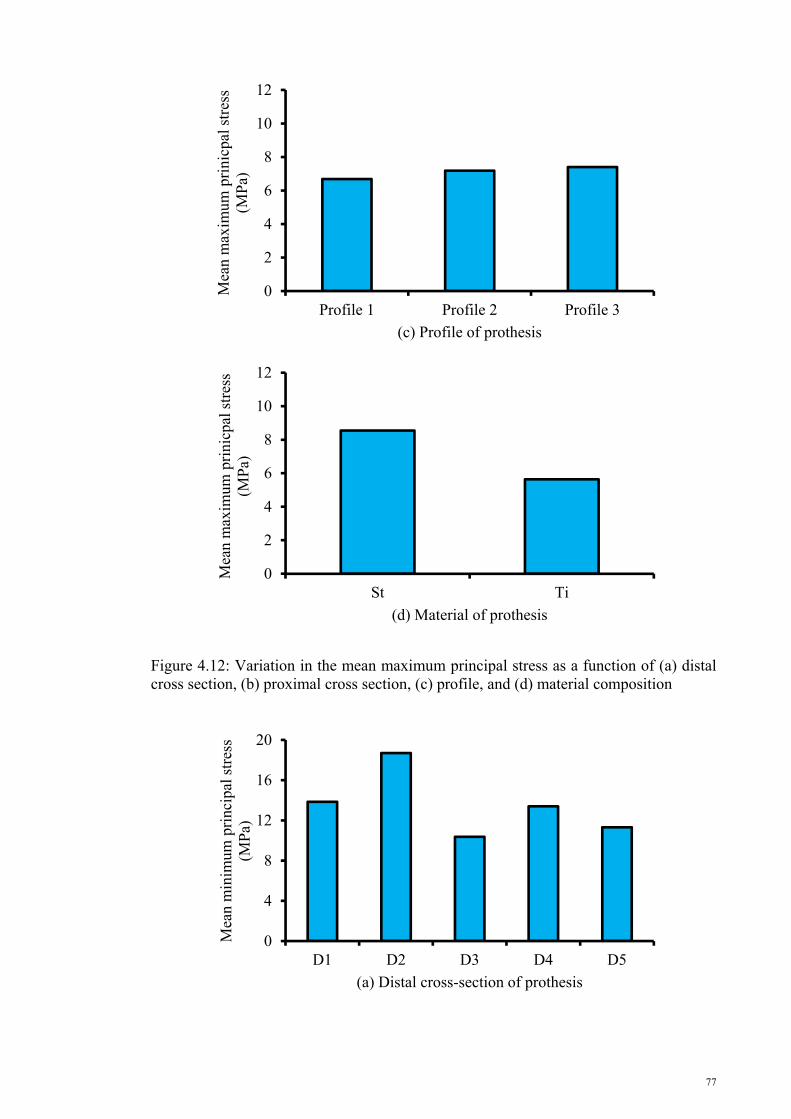
77
Figure 4.12: Variation in the mean maximum principal stress as a function of (a) distal cross section, (b) proximal cross section, (c) profile, and (d) material composition
0
2
4
6
8
10
12
Profile 1 Profile 2 Profile 3
Mea
n m
axim
um p
rini
cpal
str
ess
(MP
a)
(c) Profile of prothesis
0
2
4
6
8
10
12
St Ti
Mea
n m
axim
um p
rini
cpal
str
ess
(MP
a)
(d) Material of prothesis
0
4
8
12
16
20
D1 D2 D3 D4 D5
Mea
n m
inim
um p
rinc
ipal
str
ess
(MP
a)
(a) Distal cross-section of prothesis

78
Figure 4.13: Variation in the mean minimum principal stress variation as a function of (a) distal cross section, (b) proximal cross section, (c) profile, and (d) material composition
0
4
8
12
16
20
P1 P2 P3 P4
Mea
n m
inim
um p
rinc
ipal
str
ess
(MP
a)
(b) Proximal cross-section of prothesis
0
4
8
12
16
20
Profile 1 Profile 2 Profile 3
Mea
n m
inim
um p
rinc
ipal
str
ess
(MP
a)
(c) Profile of prothesis
0
4
8
12
16
20
St Ti
Mea
n m
inim
um p
rinc
ipal
str
ess
(MP
a)
(d) Material of prothesis

79
4.2.3 Cementless longitudinal functionally graded femoral prosthesis with different geometries
The results of applying FGMs in the femoral prostheses with different
geometries are presented in the following sections. The Young’s modulus changes in
the sagittal plane, and the prostheses geometry is composed of five different distal cross
sections, four different proximal cross sections, and three different profiles. The
simplified model of the femur was used in this FEA.
4.2.3.1 Strain energy density
Figure 4.14 illustrates the SED variation at the proximal metaphysis of the femur
for five distal cross-sections, four proximal cross-sections, three profiles, two implant–
bone interface conditions, and four gradient indices. The distal cross-sections showed
minor effect of 5.2% on SED variation (Figure 4.14a). The prostheses with proximal
cross-sections of P1 and P4 produced maximum (612.96 J/mm3) and minimum
(530.69 J/mm3) amount of SED, respectively, on the proximal metaphysis of femur
(Figure 4.14b). The prostheses with proximal cross-sections of P2 and P3 induced
almost the same SEDs of approximately 575.84 J/mm3 in the bone, which was at the
mid-range of the SED generated by the prostheses with P1and P4 proximal cross-
sections (Figure 4.14b). The prostheses developed from Profiles 1 and 3 provoked
almost the same SEDs of about 599.82 J/mm3, which was 13.0% more than the SED
induced by the prostheses with Profile 2 (521.87 J/mm3) (Figure 4.14c). The implant–
bone surface property showed insignificant effect of 0.6% on the SED variation (Figure
4.14d). The SED increased by approximately 20.2% with the increase in gradient index
from 0 to 1 (Figure 4.14e).
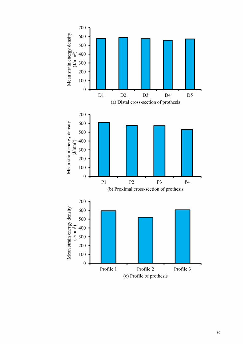
80
0
100
200
300
400
500
600
700
D1 D2 D3 D4 D5
Mea
n st
rain
ene
rgy
dens
ity
(J/m
m3 )
(a) Distal cross-section of prothesis
0
100
200
300
400
500
600
700
P1 P2 P3 P4
Mea
n st
rain
ene
rgy
dens
ity
(J/m
m3 )
(b) Proximal cross-section of prothesis
0
100
200
300
400
500
600
700
Profile 1 Profile 2 Profile 3
Mea
n st
rain
ene
rgy
dens
ity
(J/m
m3 )
(c) Profile of prothesis

81
Figure 4.14: Variation in the mean strain energy variation for the different (a) distal cross-sections, (b) proximal cross-sections, (c) profiles, (d) interface properties, and (e) gradient indices
4.2.3.2 Prostheses stress
The developed stress in the femoral prostheses is presented in Figure 4.15. The
von Mises stress behavior was similar to the SED variation with respect to the distal and
proximal cross-sections (Figures 4.15a and 4.15b). The effect of profiles on the stress
distribution in the prostheses was insignificant (0.6%). The prostheses with non-bonded
implant–bone surface condition carried 8.3% more stress than the prostheses with
0
100
200
300
400
500
600
700
µ=0.4 Bonded
Mea
n st
rain
ene
rgy
dens
ity
(J/m
m3 )
(d) Interface property
0
100
200
300
400
500
600
700
n=0 n=0.1 n=0.5 n=1
Mea
n st
rain
ene
rgy
dens
ity
(J/m
m3 )
(e) Gradient index

82
bonded implant–bone surface condition. Stress decreased by 31.9% with the increase in
gradient index from 0 to 1.
0
10
20
30
40
50
60
70
D1 D2 D3 D4 D5
Mea
n vo
n M
ises
str
ess
(MP
a)
(a) Distal cross-section of prothesis
0
10
20
30
40
50
60
70
P1 P2 P3 P4
Mea
n vo
n M
ises
str
ess
(MP
a)
(b) Proximal cross-section of prothesis

83
Figure 4.15: Variation in the mean von Mises for the different (a) distal cross-sections, (b) proximal cross-sections, (c) profiles, (d) interface properties, and (e) gradient indices
0
10
20
30
40
50
60
70
Profile 1 Profile 2 Profile 3
Mea
n vo
n M
ises
str
ess
(MP
a)
(c) Profile of prothesis
0
10
20
30
40
50
60
70
µ=0.4 Bonded
Mea
n vo
n M
ises
str
ess
(Mpa
)
(d) Interface property
0
10
20
30
40
50
60
70
n=0 n=0.1 n=0.5 n=1
Mea
n vo
n M
ises
str
ess
(MP
a)
(e) Gradient index

84
4.2.3.3 Bone Stress
The maximum and minimum principal stress variations in the bone are presented
in Figures 4.16 and 4.17. The comparison of the mean values of the principal stress
showed higher values of the minimum principal stress. The prostheses with distal cross-
sections of D1 and D2 produced almost the same maximum principal stresses in the
bone, which were greater than those of the prostheses with D3, D4, and D5. Meanwhile,
the prostheses with proximal cross-sections of P1 and P2 caused more maximum
principal stress in the bone compared with the prostheses made of proximal cross-
sections of P3 and P4. The prostheses with proximal cross-sections of P1 and P4
stimulated the highest (19.14 MPa) and the lowest (6.64 MPa) minimum principal
stresses in the femur, respectively. The effect of profiles and interface conditions on
maximum principal stress was contrary to their effects on minimum principal stress. In
other words, the prostheses with Profile 2 and non-bonded interface provoked high
maximum principal stress on the lateral side of the femur, but less minimum principal
stress on the medial side of the bone. The maximum and minimum principal stresses
showed increasing trend with the increase in gradient index. The maximum and
minimum principal stresses increased by 5.0% and 13.4%, respectively, with the
increase in gradient index from 0 to 1.

85
0
0.4
0.8
1.2
1.6
2
D1 D2 D3 D4 D5
Mea
n m
axim
um p
rinc
ipal
str
ess
(MP
a)
(a) Distal cross-section of prothesis
0
0.4
0.8
1.2
1.6
2
P1 P2 P3 P4
Mea
n m
axim
um p
rinc
ipal
str
ess
(MP
a)
(b) Proximal cross-section of prothesis
0
0.4
0.8
1.2
1.6
2
Profile 1 Profile 2 Profile 3
Mea
n m
axim
um p
rinc
ipal
str
ess
(MP
a)
(c) Profile of prothesis

86
Figure 4.16: Variation in the mean maximum principal stress for the different (a) distal cross-sections, (b) proximal cross-sections, (c) profiles, (d) interface properties, and (e) gradient indices
0
0.4
0.8
1.2
1.6
2
µ=0.4 Bonded
Mea
n m
axim
um p
rinc
ipal
str
ess
(MP
a)
(d) Interface property
0
0.4
0.8
1.2
1.6
2
n=0 n=0.1 n=0.5 n=1
Mea
n m
axim
um p
rinc
ipal
str
ess
(MP
a)
(e) Gradient index
0
4
8
12
16
20
D1 D2 D3 D4 D5
Mea
n m
inim
um p
rinc
ipal
str
ess
(MP
a)
(a) Distal cross-section of prothesis

87
0
4
8
12
16
20
P1 P2 P3 P4
Mea
n m
inim
um p
rinc
ipal
str
ess
(MP
a)
(b) Proximal cross-section of prothesis
0
4
8
12
16
20
Profile 1 Profile 2 Profile 3
Mea
n m
inim
um p
rinc
ipal
str
ess
(MP
a)
(c) Profile of prothesis
0
4
8
12
16
20
µ=0.4 Bonded
Mea
n m
inim
um p
rinc
ipal
str
ess
(MP
a)
(d) Interface property

88
Figure 4.17: Variation in the mean minimum principal stress for the different (a) distal cross-sections, (b) proximal cross-sections, (c) profiles, (d) interface properties, and (e) gradient indices
4.2.3.4 Interface stress
The interface stress behavior at the implant–bone surface is illustrated in Figure
4.18 for the non-bonded implant–bone surface. The highest and lowest values of the
interface stresses were obtained from the implant–bone surface of the implanted
prostheses with distal cross-sections of D5 (1.55 MPa) and D4 (0.28MPa), respectively.
The interface stresses caused by the prostheses with distal cross-sections of D1 and D3
were almost the same at approximately 0.64 MPa and were more than the interface
stress for the prosthesis with D4. On the contrary, the stresses for these two distal cross-
sections were less than the stresses induced by the prosthesis with D2 (0.97 MPa). The
implant–bone surface stresses caused by the implantation of the prostheses with
proximal cross-sections of P4 (0.99 MPa), P2 (0.79 MPa), P1 (0.76 MPa), and P3 (0.73
MPa) exhibited the highest to the lowest value of interface stresses. The interface stress
followed a decreasing trend at the implant–bone interface with the increase in gradient
index. The gradient index growth led to 21.7% reduction in the interface stresses.
0
4
8
12
16
20
n=0 n=0.1 n=0.5 n=1
Mea
n m
inim
um p
rinc
ipal
str
ess
(MP
a)
(e) Gradient index

89
0
0.4
0.8
1.2
1.6
2
D1 D2 D3 D4 D5
Mea
n in
terf
ace
stre
ss (
MP
a)
(a) Distal cross-section of prothesis
0
0.4
0.8
1.2
1.6
2
P1 P2 P3 P4
Mea
n in
terf
ace
stre
ss (
MP
a)
(b) Proximal cross-section of prothesis
0
0.4
0.8
1.2
1.6
2
Profile 1 Profile 2 Profile 3
Mea
n in
terf
ace
stre
ss (
MP
a)
(c) Profile of prothesis

90
Figure 4.18: Variation in the mean interface stress for the different (a) distal cross-sections, (b) proximal cross-sections, (c) profiles, and (d) gradient indices
4.2.4 Cementless radial functionally graded femoral prosthesis with different geometries
This section presents the results of inserting an implant with variable Young’s
modulus in the transverse plane in the anatomical bone. The Young’s modulus of the
prostheses increased from the cortex layer to the core of the prostheses.
4.2.4.1 Strain energy density
Figures 4.19a to 4.19d present the mean values of the SED as a function of distal
cross-section, proximal cross-section, profiles, and gradient index. The prostheses
change in the distal cross-section showed a negligible effect of 4.48% on the change in
SED. Prostheses with P1 proximal cross-section caused the maximum SED in the bone,
whereas the prostheses with P4 proximal cross-section induced the minimum SED in
the bone (Figure 4.19b). The effect of P1 on SED was 30.85% more than that of P4. The
prostheses with proximal cross-section of P2 and P3 produced almost similar SEDs in
the bone, with values between those of the prostheses with P1and P4 proximal cross-
sections (Figure 4.19b). Profiles 1 and 3 stimulated almost the same SEDs in the bone,
0
0.4
0.8
1.2
1.6
2
n=0 n=0.1 n=0.5 n=1
Mea
n in
terf
ace
stre
ss (
MP
a)
(d) Gradient index

91
which was approximately 21.52% more than that of Profile 2 (Figure 4.19c). The
increase in gradient index showed a positive impact on the change in SED (Figure
4.19d). Consequently, the prostheses with gradient indices of 1 and 0 showed the
maximum (352.2 J/mm3) and minimum (237.5 J/mm3) values of SED, respectively
(Figure 4.19d), with an approximate difference of 32.56%.
0
100
200
300
400
D1 D2 D3 D4
Mea
n st
rain
ene
rgy
dens
ity
(J/m
m3 )
(a) Distal cross-section of prothesis
0
100
200
300
400
P1 P2 P3 P4
Mea
n st
rain
ene
rgy
dens
ity
(J/m
m3 )
(b) Proximal cross-section of prothesis
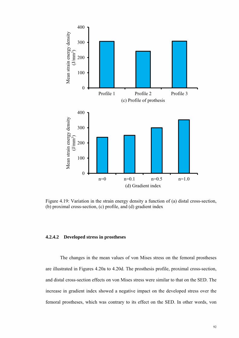
92
Figure 4.19: Variation in the strain energy density a function of (a) distal cross-section, (b) proximal cross-section, (c) profile, and (d) gradient index
4.2.4.2 Developed stress in prostheses
The changes in the mean values of von Mises stress on the femoral prostheses
are illustrated in Figures 4.20a to 4.20d. The prosthesis profile, proximal cross-section,
and distal cross-section effects on von Mises stress were similar to that on the SED. The
increase in gradient index showed a negative impact on the developed stress over the
femoral prostheses, which was contrary to its effect on the SED. In other words, von
0
100
200
300
400
Profile 1 Profile 2 Profile 3
Mea
n st
rain
ene
rgy
dens
ity
(J/m
m3 )
(c) Profile of prothesis
0
100
200
300
400
n=0 n=0.1 n=0.5 n=1.0
Mea
n st
rain
ene
rgy
dens
ity
(J/m
m3 )
(d) Gradient index

93
Mises stress on femoral prostheses declined with the increase in gradient index (Figure
4.20d). Consequently, prostheses with gradient indices of 1 and 0 induced the minimum
and maximum von Mises stresses, respectively. The gradient index, profile, proximal
cross-section, and distal cross-section caused corresponding differences of 79.06%,
7.97%, 20.82%, and 5.60% between the maximum and minimum mean von Mises
stresses at the prostheses.
0
20
40
60
80
100
D1 D2 D3 D4
Mea
n vo
n M
ises
str
ess
(MP
a)
(a) Distal cross-section of prothesis
0
20
40
60
80
100
P1 P2 P3 P4
Mea
n vo
n M
ises
str
ess
(MP
a)
(b) Proximal cross-section of prothesis

94
Figure 4.20: Variation in the von Mises stress as a function of (a) distal cross-section, (b) proximal cross-section, (c) profile, and (d) gradient index
4.2.4.3 Developed stress in the bone
The variations in the mean values of the developed maximum and minimum principal
stresses in the bone as functions of distal cross-section, proximal cross-section, profile,
and gradient index are presented in Figures 4.21a to 4.22d. A negligible effect was
observed in the maximum principal stress caused by the change in all considered
parameters (Figures 4.21a to 4.21d). The maximum and minimum principal stresses
increased with gradient index (Figures 4.21d and 4.22d). The developed maximum
principal stress in the bone attributed to the implantation of the prostheses with Profile 2
0
20
40
60
80
100
Profile 1 Profile 2 Profile 3
Mea
n vo
n M
ises
str
ess
(MP
a)
(c) Profile of prothesis
0
20
40
60
80
100
n=0 n=0.1 n=0.5 n=1.0
Mea
n vo
n M
ises
str
ess
(MP
a)
(d) Gradient index

95
was approximately 2.0% more than that attributed to the implantation of the prostheses
with Profiles 1 and 3. The effects of both proximal and distal cross-sections on the
maximum and minimum principal stresses were insignificant. The average effect of the
distal and proximal cross-sections on the maximum and minimum principal stresses was
5.4%, whereas the average effect of the gradient index growth on the maximum and
minimum principal stresses was 13.6%.
0
2
4
6
8
10
D1 D2 D3 D4
Mea
n m
axim
um p
rinc
ipal
str
ess
(MP
a)
(a) Distal cross-section of prothesis
0
2
4
6
8
10
P1 P2 P3 P4
Mea
n m
axim
um p
rinc
ipal
str
ess
(MP
a)
(b) Proximal cross-section of prothesis

96
Figure 4.21: Variation in the maximum principal stress as a function of (a) distal cross-section, (b) proximal cross-section, (c) profile, and (d) gradient index
0
2
4
6
8
10
Profile 1 Profile 2 Profile 3
Mea
n m
axim
um p
rinc
ipal
str
ess
(MP
a)
(c) Profile of prothesis
0
2
4
6
8
10
n=0 n=0.1 n=0.5 n=1.0Mea
n m
axim
um p
rinc
ipal
str
ess
(MP
a)
(d) Gradient index
0
2
4
6
8
10
12
D1 D2 D3 D4
Mea
n M
inim
um P
rinc
ipal
str
ess
(MP
a)
(a) Distal cross-section of prothesis

97
Figure 4.22: Variation in the minimum principal stress as a function of (a) distal cross-section, (b) proximal cross-section, (c) profile, and (d) gradient index
0
2
4
6
8
10
12
P1 P2 P3 P4
Mea
n M
inim
um P
rinc
ipal
str
ess
(MP
a)
(b) Proximal cross-section of prothesis
0
2
4
6
8
10
12
Profile 1 Profile 2 Profile 3
Mea
n M
inim
um P
rinc
ipal
str
ess
(MP
a)
(c) Profile of prothesis
0
2
4
6
8
10
12
n=0.0 n=0.1 n=0.5 n=1.0
Mea
n M
inim
um P
rinc
ipal
str
ess
(MP
a)
(d) Gradient index

98
4.2.4.4 Interface Stress
The interface stress variations at the implant–bone interface are illustrated in
Figures 4.23a to 4.23d. The maximum and minimum interface stresses were observed
with the implantation of the prostheses with D2 and D3 distal cross-sections,
respectively. The D1 and D4 distal cross-sections showed a similar effect on the
interface stresses. The distal cross-sections caused a 60.09% difference between the
maximum and minimum mean interface stresses. As shown in Figure 4.23b, the
prostheses with the maximum to minimum interface stresses are those with proximal
cross-sections of P3, P2, P1, and P4, and a 34.23% difference was observed between the
minimum and maximum mean interface stresses. The interface stresses displayed an
increasing trend with the change from Profiles 1 to 3 (Figure 4.23c). The difference
between the change in the maximum and minimum interface stress that was attributed to
the profiles was 40.90%. The interface stresses decreased with the gradient index
(Figure 4.23d). The maximum interface stress emerged in the implant–bone interface
because of the prostheses with gradient index of 0, and the minimum interface stress
resulted from the prostheses with gradient index of 1 (Figure 4.23d). The mean interface
stress reduction was 62.44% caused by the increase in gradient index from 0 to 1.

99
0
6
12
18
24
30
D1 D2 D3 D4
Mea
n in
terf
ace
stre
ss (
MP
a)
(a) Distal cross-section of prothesis
0
6
12
18
24
30
P1 P2 P3 P4
Mea
n in
terf
ace
stre
ss (
MP
a)
(b) Proximal cross-section of prothesis
0
6
12
18
24
30
Profile 1 Profile 2 Profile 3
Mea
n in
terf
ace
stre
ss (
MP
a)
(c) Profile of prothesis

100
Figure 4.23: Variation in the interface stress as a function of (a) distal cross-section, (b) proximal cross-section, (c) profile, and (d) gradient index
0
6
12
18
24
30
n=0 n=0.1 n=0.5 n=1.0
Mea
n in
terf
ace
stre
ss (
MP
a)
(d) Gradient index

101
4.2.5 Cemented prostheses with conventional materials
This section presents the FEA results of the anatomical femur implanted with
different cemented prostheses composed of conventional materials of St and Ti.
4.2.5.1 Strain energy density
Figures 4.24a to 4.24d illustrate the variation in the SED in the proximal
metaphysis of femur as a function of distal cross-section, proximal cross-section,
profile, and material. Among the prostheses with different distal cross-sections, the
prostheses with distal cross-sections of D1 and D4 provoked about 7.8% more SED in
the bone. The prostheses with distal cross-section of D3 produced the minimum SED of
280.84 J/mm3 in the bone. The prostheses with P1 proximal cross-section induced 4.5%
and 8.4% more SED than the prostheses with P2 and P3 proximal cross-sections,
respectively. The prostheses with Profiles 3, 1, and 2 caused the highest SED to the
lowest SEDs of 316.53, 308.58, and 259.13 J/mm3 in the bone, respectively. Meanwhile,
the Ti-based prostheses stimulated 31.0% more SED in the bone than the St-based
prostheses.
0
80
160
240
320
400
D1 D2 D3 D4
Mea
n st
rain
ene
rgy
dens
ity
(J/m
m3 )
(a) Distal cross-section of prothesis

102
Figure 4.24: Strain energy density as a function of the (a) distal cross-section, (b) proximal cross-section, (c) profile, and (d) material of the prostheses
0
80
160
240
320
400
P1 P2 P3
Mea
n st
rain
ene
rgy
dens
ity
(J/m
m3 )
(b) Proximal cross-section of prothesis
0
80
160
240
320
400
Profile 1 Profile 2 Profile 3
Mea
n st
rain
ene
rgy
dens
ity
(J/m
m3 )
(c) Profile of prothesis
0
80
160
240
320
400
St Ti
Mea
n st
rain
ene
rgy
dens
ity
(J/m
m3 )
(d) Material of prothesis

103
4.2.5.2 Developed stress in the prostheses
The von Mises stress variations at the lateral and medial sides of prostheses
composed of conventional materials as functions of distal cross-section, proximal cross-
section, profile, and material are illustrated in Figure 4.25. As shown in Figure 4.25, the
medial side of prostheses exhibited 21.8% more stress compared with the lateral side.
Geometrical parameters showed minor effect of 7.8% on the prostheses stress variation
(Figures 4.25a to 4.25c). On the contrary, the material of the prostheses demonstrated
more effect on stress, and the St-based prostheses tolerated 30.9% more stress than the
Ti-based prostheses (Figure 4.25d).
0
20
40
60
80
100
120
140
D1 D2 D3 D4
Mea
n vo
n M
ises
str
ess
(MP
a)
(a) Distal cross-section of prothesis
Lateral Medial
0
20
40
60
80
100
120
140
P1 P2 P3
Mea
n vo
n M
ises
str
ess
(MP
a)
(b) Proximal cross-section of prothesis
Lateral Medial
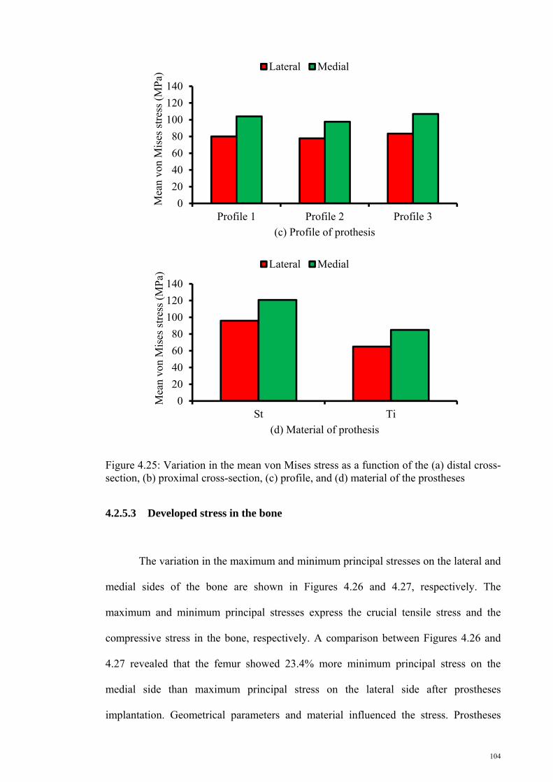
104
Figure 4.25: Variation in the mean von Mises stress as a function of the (a) distal cross-section, (b) proximal cross-section, (c) profile, and (d) material of the prostheses
4.2.5.3 Developed stress in the bone
The variation in the maximum and minimum principal stresses on the lateral and
medial sides of the bone are shown in Figures 4.26 and 4.27, respectively. The
maximum and minimum principal stresses express the crucial tensile stress and the
compressive stress in the bone, respectively. A comparison between Figures 4.26 and
4.27 revealed that the femur showed 23.4% more minimum principal stress on the
medial side than maximum principal stress on the lateral side after prostheses
implantation. Geometrical parameters and material influenced the stress. Prostheses
0
20
40
60
80
100
120
140
Profile 1 Profile 2 Profile 3
Mea
n vo
n M
ises
str
ess
(MP
a)
(c) Profile of prothesis
Lateral Medial
0
20
40
60
80
100
120
140
St Ti
Mea
n vo
n M
ises
str
ess
(MP
a)
(d) Material of prothesis
Lateral Medial

105
with distal cross-section of D2, proximal cross-section of P2, and Profile 2 provoked
more maximum principal stress in the bone, whereas prostheses composed of D4 distal
cross-section, P3 proximal cross-section, and Profile 2 caused more minimum principal
stress in the bone. The profile effect on the minimum principal stress was negligible
(2.7%). Meanwhile, the Ti-based prostheses induced 10.5% more maximum principal
stress and 1.8% more minimum principal stress in the bone than the St-based prostheses
(Figures 4.26d and 4.27d).
0
4
8
12
16
20
D1 D2 D3 D4
Mea
n m
axim
um p
rinc
ipal
str
ess
(MP
a)
(a) Distal cross-section of prothesis
0
4
8
12
16
20
P1 P2 P3
Mea
n m
axim
um p
rinc
ipal
str
ess
(MP
a)
(b) Proximal cross-section of prothesis

106
Figure 4.26: Variation in the mean maximum principal stress as a function of the (a) distal cross-section, (b) proximal cross-section, (c) profile, and (d) material of the prostheses
0
4
8
12
16
20
Profile 1 Profile 2 Profile 3
Mea
n m
axim
um p
rinc
ipal
str
ess
(MP
a)
(c) Profile of prothesis
0
4
8
12
16
20
St Ti
Mea
n m
axim
um p
rinc
ipal
str
ess
(MP
a)
(d) Material of prothesis
0
4
8
12
16
20
D1 D2 D3 D4
Mea
n m
inim
um p
rinc
ipal
str
ess
(MP
a)
(a) Distal cross-section of prothesis

107
Figure 4.27: Variation in the mean minimum principal stress as a function of the (a) distal cross-section, (b) proximal cross-section, (c) profile, and (d) material of the prostheses
0
4
8
12
16
20
P1 P2 P3
Mea
n m
inim
um p
rinc
ipal
str
ess
(MP
a)
(b) Proximal cross-section of prothesis
0
4
8
12
16
20
Profile 1 Profile 2 Profile 3
Mea
n m
inim
um p
rinc
ipal
str
ess
(MP
a)
(c) Profile of prothesis
0
4
8
12
16
20
St Ti
Mea
n m
inim
um p
rinc
ipal
str
ess
(MP
a)
(d) Material of prothesis
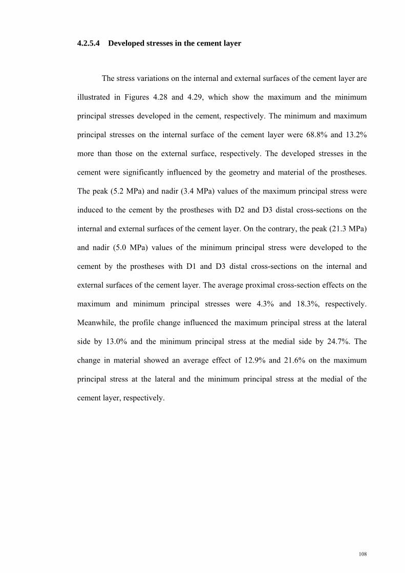
108
4.2.5.4 Developed stresses in the cement layer
The stress variations on the internal and external surfaces of the cement layer are
illustrated in Figures 4.28 and 4.29, which show the maximum and the minimum
principal stresses developed in the cement, respectively. The minimum and maximum
principal stresses on the internal surface of the cement layer were 68.8% and 13.2%
more than those on the external surface, respectively. The developed stresses in the
cement were significantly influenced by the geometry and material of the prostheses.
The peak (5.2 MPa) and nadir (3.4 MPa) values of the maximum principal stress were
induced to the cement by the prostheses with D2 and D3 distal cross-sections on the
internal and external surfaces of the cement layer. On the contrary, the peak (21.3 MPa)
and nadir (5.0 MPa) values of the minimum principal stress were developed to the
cement by the prostheses with D1 and D3 distal cross-sections on the internal and
external surfaces of the cement layer. The average proximal cross-section effects on the
maximum and minimum principal stresses were 4.3% and 18.3%, respectively.
Meanwhile, the profile change influenced the maximum principal stress at the lateral
side by 13.0% and the minimum principal stress at the medial side by 24.7%. The
change in material showed an average effect of 12.9% and 21.6% on the maximum
principal stress at the lateral and the minimum principal stress at the medial of the
cement layer, respectively.

109
0
1
2
3
4
5
6
D1 D2 D3 D4Mea
n m
axim
um p
rinc
ipal
str
ess
(MP
a)
(a) Distal cross-section of prothesis
Internal External
0
1
2
3
4
5
6
P1 P2 P3Mea
n m
axim
um p
rinc
ipal
str
ess
(MP
a)
(b) Proximal cross-section of prothesis
Internal External
0
1
2
3
4
5
6
Profile 1 Profile 2 Profile 3
Mea
n m
axim
um p
rinc
ipal
str
ess
(MP
a)
(c) Profile of prothesis
Internal External

110
Figure 4.28: Variation in the mean maximum principal stress as a function of the (a) distal cross-section, (b) proximal cross-section, (c) profile, and (d) material of the prostheses
0
1
2
3
4
5
6
St Ti
Mea
n m
axim
um p
rinc
ipal
str
ess
(MP
a)
(d) Material of prothesis
Internal External
0
5
10
15
20
25
D1 D2 D3 D4
Mea
n m
inim
um p
rinc
ipal
str
ess
(MP
a)
(a) Distal cross-section of prothesis
Internal External
0
5
10
15
20
25
P1 P2 P3
Mea
n m
inim
um p
rinc
ipal
str
ess
(MP
a)
(b) Proximal cross-section of prothesis
Internal External

111
Figure 4.29: Variation in the mean minimum principal stress as a function of the (a) distal cross-section, (b) proximal cross-section, (c) profile, and (d) material of the prostheses
4.2.6 Radial and longitudinal cemented functionally graded prostheses
The results of FEA on cemented FG RPs and LPs are presented in the following
section.
4.2.6.1 Strain energy density
The SED values were derived from FEA results and plotted as bar charts in the
two groups on the basis of the implanted RP and LP. Figure 4.30 shows the variation in
0
5
10
15
20
25
Profile 1 Profile 2 Profile 3
Mea
n m
inim
um p
rinc
ipal
str
ess
(MP
a)
(c) Profile of prothesis
Internal External
0
5
10
15
20
25
St Ti
Mea
n m
inim
um p
rinc
ipal
str
ess
(MP
a)
(d) Material of prothesis
Internal External

112
the SED for different distal cross-sections. The prostheses with distal cross-section of
D2 exhibited 7.8% more SED than the other prostheses in both group of FG RPs and
LPs, whereas the prostheses with distal cross-section of D3 produced minimum SED
(386.61 J/mm3 for RP and 372.19 J/mm3 for LP) in the proximal metaphysis of femur in
both groups. The prostheses with proximal cross-sections of P1 and P3 caused
maximum SEDs of 434.80 (RP) and 407.26 J/mm3 (LP) and minimum SEDs of 391.27
(RP) and 371.80 J/mm3 (LP) in the bone. The prostheses with Profile 2 induced
maximum SED of 408.68 J/mm3 in the proximal metaphysis of femur in RP, whereas
the prostheses with Profile 2 provoked minimum SED of 383.60 J/mm3 in the bone by
LPs. The SED increased by approximately 24.6% with the increase in gradient index in
both groups similar to cementless prostheses. The RPs provoked 8.3% more SED in the
bone compared with the LPs.
0
100
200
300
400
500
RP LP
Mea
n st
rain
ene
rgy
dens
ity
(J/m
m3 )
(a) Prosthesis type
D1 D2 D3 D4

113
Figure 4.30: Variation in the strain energy density at the different (a) distal cross-sections, (b) proximal cross-sections, (c) profiles, and (d) gradient indices
0
100
200
300
400
500
RP LP
Mea
n st
rain
ene
rgy
dens
ity
(J/m
m3 )
(b) Prosthesis type
P1 P2 P3
0
100
200
300
400
500
RP LP
Mea
n st
rain
ene
rgy
dens
ity
(J/m
m3 )
(c) Prosthesis type
Profile 1 Profile 2 Profile 3
0
100
200
300
400
500
RP LP
Mea
n st
rain
ene
rgy
dens
ity
(J/m
m3 )
(d) Prosthesis type
n=0 n=0.1 n=0.5 n=1.0

114
4.2.6.2 Developed stress in the prostheses
The developed von Mises stress on the lateral and medial sides of the femoral
prostheses are presented in Figure 4.31. The developed stress presented in bar charts are
divided into four groups, namely, the lateral side of radial femoral prostheses (LRP),
lateral side of longitudinal prostheses (LLP), medial side of radial prostheses (MRP),
and medial side of longitudinal prostheses (MLP). The medial side of prostheses in both
groups of cemented prostheses endured approximately 28.0% more stress. The
prostheses with D2 and D3 distal cross-sections exhibited the maximum and minimum
von Mises stresses, respectively. The von Mises stress declined with the increase in
gradient index from 0 to 1 at the LRP, LLP, MRP, and MLP by approximately 71.4%,
27.0%, 54.2%, and 26.0%, respectively.
0
30
60
90
LRP LLP MRP MLP
Mea
n vo
n M
ises
str
ess
(MP
a)
(a) Prosthesis side and type
D1 D2 D3 D4
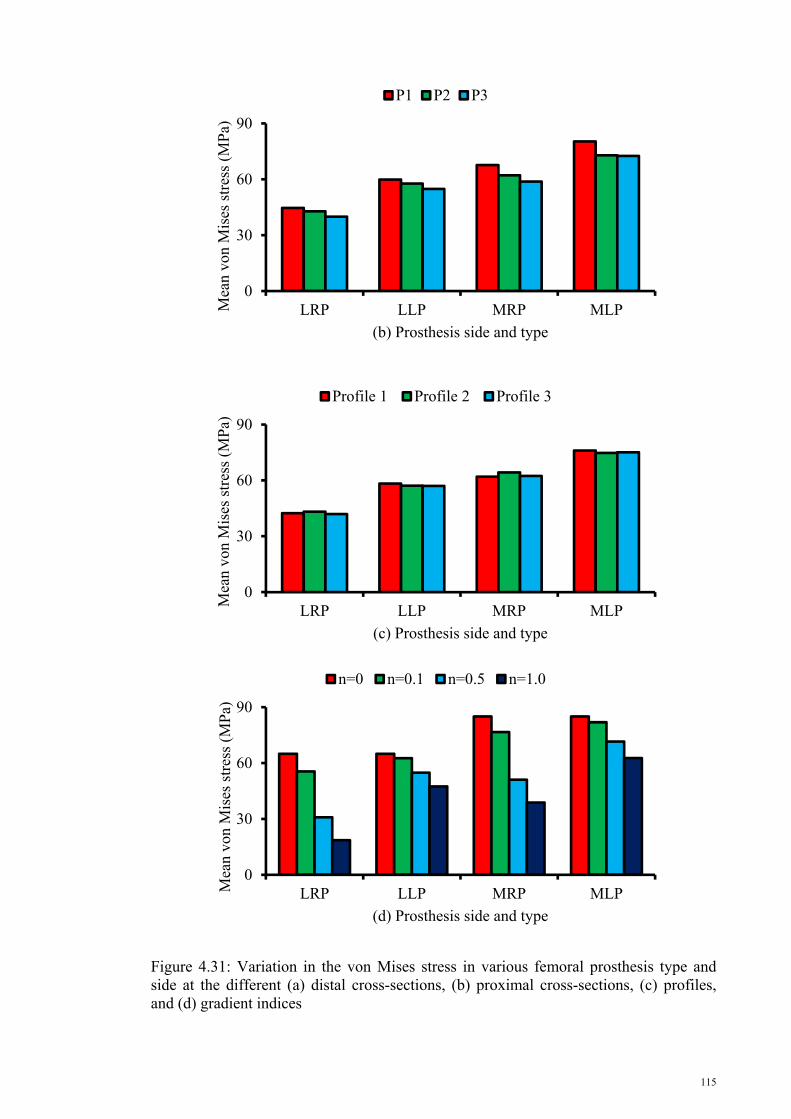
115
Figure 4.31: Variation in the von Mises stress in various femoral prosthesis type and side at the different (a) distal cross-sections, (b) proximal cross-sections, (c) profiles, and (d) gradient indices
0
30
60
90
LRP LLP MRP MLPMea
n vo
n M
ises
str
ess
(MP
a)
(b) Prosthesis side and type
P1 P2 P3
0
30
60
90
LRP LLP MRP MLP
Mea
n vo
n M
ises
str
ess
(MP
a)
(c) Prosthesis side and type
Profile 1 Profile 2 Profile 3
0
30
60
90
LRP LLP MRP MLPMea
n vo
n M
ises
str
ess
(MP
a)
(d) Prosthesis side and type
n=0 n=0.1 n=0.5 n=1.0

116
4.2.6.3 Developed stress in the bone
The mean values of the maximum principal stress at the lateral side and the
minimum principal stress at the medial side of the femur are presented in Figures 4.32
and 4.33, respectively. The femur carried more maximum principal stress by the
implantation of prostheses with D2 distal cross-section, P2 proximal cross-section, and
Profile 2 regardless of radial or longitudinal change in Young’s modulus. The stress
also showed an increasing trend with the increase in gradient index.
0
3
6
9
12
15
18
RP LP
Mea
n m
axim
um p
rinc
ipal
str
ess
(MP
a)
(a) Implanted prosthesis
D1 D2 D3 D4
0
3
6
9
12
15
18
RP LPMea
n m
axim
um p
rinc
ipal
str
ess
(MP
a)
(b) Implanted prosthesis
P1 P2 P3

117
Figure 4.32: Variation in the maximum principal stress at the lateral side of femur at the different (a) distal cross-sections, (b) proximal cross-sections, (c) profiles, and (d) gradient indices
As shown in Figure 4.33, the prostheses with D2 and D4 distal cross-sections
induced more minimum principal stress in the bone. By contrast, with the maximum
principal stress, the prostheses with P2 proximal cross-section and Profile 2 caused less
minimum principal stress in the bone. The minimum principal stress increased with the
increase in gradient index. However, the minimum principal stress growth caused by the
gradient index increase for the implantation of LP was less than that of RP.
0
3
6
9
12
15
18
RP LPMea
n m
axim
um p
rinc
ipal
str
ess
(MP
a)
(c) Implanted prosthesis
Profile 1 Profile 2 Profile 3
0
3
6
9
12
15
18
RP LP
Mea
n m
axim
um p
rinc
ipal
str
ess
(MP
a)
(d) Implanted prosthesis
n=0 n=0.1 n=0.5 n=1.0

118
0
4
8
12
16
20
RP LP
Mea
n m
inim
um p
rinc
ipal
str
ess
(MP
a)
(a) Implanted prosthesis
D1 D2 D3 D4
0
4
8
12
16
20
RP LPMea
n m
inim
um p
rinc
ipal
str
ess
(MP
a)
(b) Implanted prosthesis
P1 P2 P3
0
4
8
12
16
20
RP LPMea
n m
inim
um p
rinc
ipal
str
ess
(MP
a)
(c) Implanted prosthesis
Profile 1 Profile 2 Profile 3

119
Figure 4.33: Variation in the minimum principal stress at the lateral side of the femur at the different (a) distal cross-sections, (b) proximal cross-sections, (c) profiles, and (d) gradient indices
4.2.7 Developed stress in the cement
The maximum principal stresses developed at the lateral side on the internal and
external surface of the cement because of the implantation of FG LP and RP are
illustrated in Figure 4.34. RP induced approximately 10.7% more maximum principal
stress in the cement than LP. The internal surface of the cement layer in RP carried
15.5% more maximum principal stress than the external surface, whereas the external
surface in LP tolerated 3.5% more maximum principal stress than the internal surface.
The prostheses with D2 cross-section stimulated higher stress in the cement than the
prostheses with other distal cross-sections. RP with Profile 2 produced more maximum
principal stress, whereas LP with Profile 1 induced less maximum principal stress in
cement. The increase in gradient index led to the increase in the maximum principal
stress in LP and RP by approximately 17.5% and 6.2%, respectively.
0
4
8
12
16
20
RP LPMea
n m
inim
um p
rinc
ipal
str
ess
(MP
a)
(d) Implanted prosthesis
n=0 n=0.1 n=0.5 n=1.0

120
01234567
Internalsurface-RP
Externalsurface-RP
Internalsurface-LP
Externalsurface-LP
Mea
n m
axim
um p
rinc
ipal
str
ess
(MP
a)
(a) Cement surface and implanted prosthesis
D1 D2 D3 D4
01234567
Internalsurface-RP
Externalsurface-RP
Internalsurface-LP
Externalsurface-LP
Mea
n m
axim
um p
rinc
ipal
str
ess
(MP
a)
(b) Cement surface and implanted prosthesis
P1 P2 P3
01234567
Internalsurface-RP
Externalsurface-RP
Internalsurface-LP
Externalsurface-LPM
ean
max
imum
pri
ncip
al s
tres
s (M
Pa)
(c) Cement surface and implanted prosthesis
Profile 1 Profile 2 Profile 3
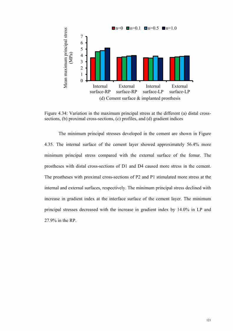
121
Figure 4.34: Variation in the maximum principal stress at the different (a) distal cross-sections, (b) proximal cross-sections, (c) profiles, and (d) gradient indices
The minimum principal stresses developed in the cement are shown in Figure
4.35. The internal surface of the cement layer showed approximately 56.4% more
minimum principal stress compared with the external surface of the femur. The
prostheses with distal cross-sections of D1 and D4 caused more stress in the cement.
The prostheses with proximal cross-sections of P2 and P1 stimulated more stress at the
internal and external surfaces, respectively. The minimum principal stress declined with
increase in gradient index at the interface surface of the cement layer. The minimum
principal stresses decreased with the increase in gradient index by 14.0% in LP and
27.9% in the RP.
01234567
Internalsurface-RP
Externalsurface-RP
Internalsurface-LP
Externalsurface-LP
Mea
n m
axim
um p
rinc
ipal
str
ess
(MP
a)
(d) Cement surface & implanted prosthesis
n=0 n=0.1 n=0.5 n=1.0

122
0
4
8
12
16
20
Internal surface-RP
External surface-RP
Internal surface-LP
External surface-LP
Mea
n m
inim
um p
rinc
ipal
str
ess
(MP
a)
(a) Cement surface and implanted prosthesis
D1 D2 D3 D4
0
4
8
12
16
20
Internal surface-RP
External surface-RP
Internal surface-LP
External surface-LP
Mea
n m
inim
um p
rinc
ipal
str
ess
(MP
a)
(b) Cement surface and implanted prosthesis
P1 P2 P3
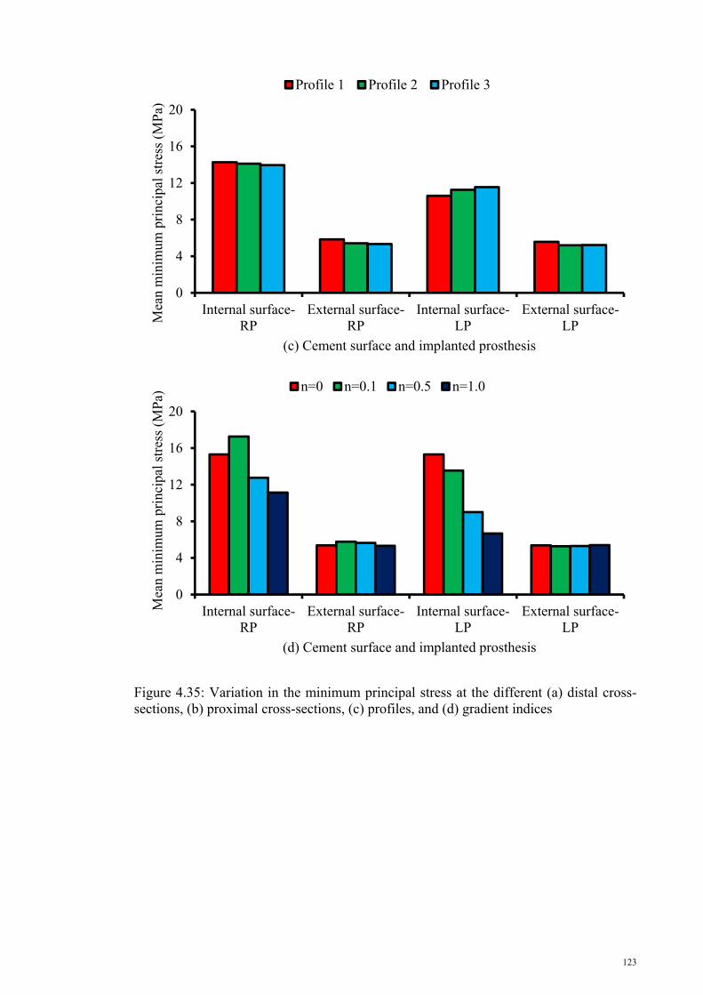
123
Figure 4.35: Variation in the minimum principal stress at the different (a) distal cross-sections, (b) proximal cross-sections, (c) profiles, and (d) gradient indices
0
4
8
12
16
20
Internal surface-RP
External surface-RP
Internal surface-LP
External surface-LPM
ean
min
imum
pri
ncip
al s
tres
s (M
Pa)
(c) Cement surface and implanted prosthesis
Profile 1 Profile 2 Profile 3
0
4
8
12
16
20
Internal surface-RP
External surface-RP
Internal surface-LP
External surface-LP
Mea
n m
inim
um p
rinc
ipal
str
ess
(MP
a)
(d) Cement surface and implanted prosthesis
n=0 n=0.1 n=0.5 n=1.0

124
4.2.8 Circumferential cracks in cement
Cracks at the cement–femoral prosthesis interface or cement–bone interface
endanger the femoral prosthesis stability, which can ultimately cause the THR to
collapse. Therefore, circumferential cracks were examined for the cemented implanted
femur, and the SIFs were measured along the crack front in the cement layer. The
findings are presented in this section. SIFs are plotted as a function of crack front length
in a counterclockwise path, with start point at the corner of the lateral posterior in the
five main phases of gait: heel strike, single-leg stance, push off, toe off, and swing
phase commencement. The presented results were divided into the SIFs for internal,
external, and internal–external cracks.
4.2.8.1 Internal circumferential crack
4.2.8.1.1 KI behavior
Figure 4.36 shows the variation in KI along the crack front in different gait
phases. KI manifested the same trend in all gait phases regardless of the crack location.
KI in all sections (25, 50, 75, and 100 mm) and in three gait stages (single-leg stance,
toe off, and push off) commenced and finalized at the maximum values, with minimum
SIFs at the middle of the crack front length. In addition, the heel strike and swing
phases demonstrated an almost sinusoidal behavior with opposite trends. The maximum
absolute values of KI for all crack models occurred in the single-leg stance and push off
phases. However, the minimum absolute KI value was recorded during the swing phase.
The absolute minimum and maximum values of the KI steadily declined along
the length of the cement mantle (z direction) except for KI,C100, which presented an

125
unexpected positive trend compared with KI,C75 because of the increase in the induced
stress to the cement at the beneath of the prosthesis neck. KI decreased during the heel
strike (89.5%), single-leg stance (91.2%), push off (87.6%), toe off (86.8%), and swing
(88.6%) phases at the lateral side of the cement layer. Moreover, the absolute values of
KI in the medial side of the cement layer in the heel strike, single-leg stance, push off,
and toe off declined by approximately 69.4%, 51.4%, 47.3%, and 61.5%, respectively.
Figure 4.36: KI variation along the crack front length at different crack locations: (a) 25, (b) 50, (c) 75, and (d) 100 mm
(a) (b)
(c) (d)
Str
ess
inte
nsit
y fa
ctor
, KII (
MP
a.m
m1/
2 )
Crack front length (mm)

126
4.2.8.1.2 KII behavior
Figure 4.37 shows the KII variations versus the crack front length. KII evidently
fluctuated along the crack front length with the highest peak at the middle of the graph.
Meanwhile, the peak amplitude of the graphs slightly increased with movement toward
the distal end.
Figure 4.37: KII variations along the crack front length at different crack locations: (a) 25, (b) 50, (c) 75, and (d) 100 mm
4.2.8.1.3 KIII behavior
Figure 4.38 illustrates the KIII behavior along the crack front. It shows a similar
sinusoidal graph in different gait phases at four various levels. The three gait phases
(push off, single-leg stance, and toe off) presented descending amplitudes in the z
direction. The SIFs in the swing phase graph fluctuated with nearly the same trends in
(a) (b)
(c) (d)
Str
ess
inte
nsit
y fa
ctor
, KII (
MP
a.m
m1/
2 )
Crack front length (mm)

127
all sections. However, the heel strike phase exhibited a sinusoidal behavior with a
length lag from the starting points and a decreasing amplitude along the z direction.
Based on the graph, the values of KIII decreased during gait, along with the
increasing distance from the distal end at the anterior during the heel strike (73.1%),
single-leg stance (80.0%), push off (73.0%), toe off (75.0%), and swing (28.6%) phases.
Similarly, at the posterior side of the cement layer, the absolute values of KIII declined
by 68.4%, 70.0%, 67.6%, 76.2%, and 0.0% during the heel strike, single-leg stance,
push off, toe off, and swing phases, respectively.
Figure 4.38: KIII variation along the crack front length at different crack locations: (a) 25, (b) 50, (c) 75, and (d) 100 mm
(a) (b)
(c) (d)
Str
ess
inte
nsit
y fa
ctor
, KII
I (M
Pa.
mm
1/2 )
Crack front length (mm)

128
4.2.8.2 External circumferential crack
4.2.8.2.1 KI Behavior
Figure 4.39 presents the KI variations for the external circumferential crack as a
function of crack front length. The trend of SIFs for the external crack along the crack
front was similar to the SIF behavior at the crack front in the internal circumferential
cracks. The highest values of SIFs were observed in the distal part, and SIFs decreased
toward the proximal portion of the cement layer.
Figure 4.39: KI variation along the crack front length at different crack locations: (a) 25, (b) 50, (c) 75, and (d) 100 mm
(a) (b)
(c) (d)
Str
ess
inte
nsit
y fa
ctor
, KI (
MP
a.m
m1/
2 )
Crack front length (mm)

129
4.2.8.2.2 KII behavior
KII trend as a function of crack front length is portrayed in Figure 4.40.
Compared with the KI values, the KII values were small and close to zero, similar to the
KII in internal circumferential cracks. The KII close to the distal and proximal ends
showed peaks in single-leg stance and push off phases.
Figure 4.40: KII variation along the crack front length at different crack locations (a) 25, (b) 50, (c) 75, and (d) 100 mm
4.2.8.2.3 KIII behavior
The KIII variations along the crack front length were plotted and presented in
Figure 4.41. KIII for external crack showed a trend similar to that of KIII at the internal
surface of the cement layer. Similar to KI, KIII had maximum values in the distal portion
(a) (b)
(c) (d)
Str
ess
inte
nsit
y fa
ctor
, KII (
MP
a.m
m1/
2 )
Crack front length (mm)
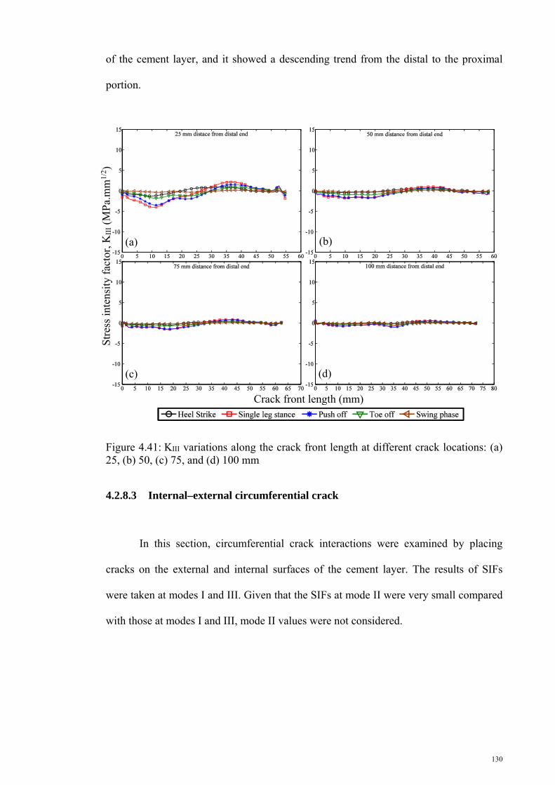
130
of the cement layer, and it showed a descending trend from the distal to the proximal
portion.
Figure 4.41: KIII variations along the crack front length at different crack locations: (a) 25, (b) 50, (c) 75, and (d) 100 mm
4.2.8.3 Internal–external circumferential crack
In this section, circumferential crack interactions were examined by placing
cracks on the external and internal surfaces of the cement layer. The results of SIFs
were taken at modes I and III. Given that the SIFs at mode II were very small compared
with those at modes I and III, mode II values were not considered.
(a) (b)
(c) (d)
Str
ess
inte
nsit
y fa
ctor
, KII
I (M
Pa.
mm
1/2 )
Crack front length (mm)

131
4.2.8.3.1 KI behavior at the internal and external surfaces
The SIF behavior at the crack front for the interaction of the internal and
external cracks is illustrated in Figures 4.42 and 4.43. In the figure title, the first number
signifies the crack position at the internal surface, and the second number shows the
location of the crack on the external surface of the cement layer. The KI for the cracks at
different positions, regardless of internal or external location, started from a maximum
value and gradually decreased to a minimum value. Afterward, the KI trend increased to
the end of the crack front. The KI variations along the crack front created concave plots
except at the heel strike phase. The KI behavior plot along the crack front in the heel
strike phase at the internal surface comprised convex and concave plots. The KI
behavior in the heel strike phase on the external surface created concave and convex
plots. The single-leg stance and push off phases had the maximum absolute values of KI
among the different phases of gait cycles. In addition, the absolute value of KI decreased
by attaining distance from the distal end.
Str
ess
inte
nsit
y fa
ctor
, KI (
MP
a.m
m1/
2 )
Crack front length (mm)
(a)
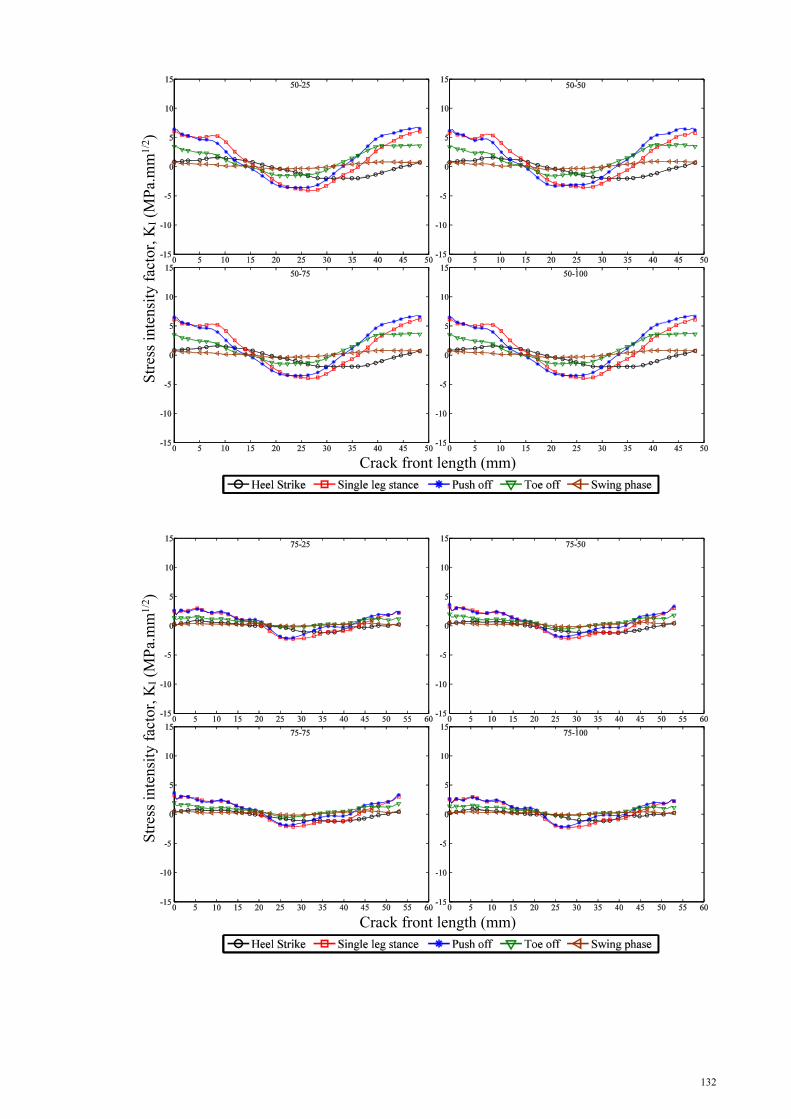
132
Str
ess
inte
nsit
y fa
ctor
, KI (
MP
a.m
m1/
2 )
Crack front length (mm)
(b)
Str
ess
inte
nsit
y fa
ctor
, KI (
MP
a.m
m1/
2 )
Crack front length (mm)
(c)
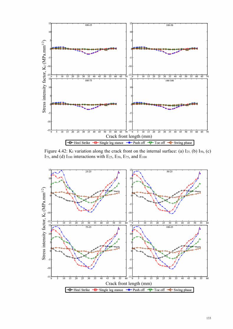
133
Figure 4.42: KI variation along the crack front on the internal surface: (a) I25, (b) I50, (c) I75, and (d) I100 interactions with E25, E50, E75, and E100
Str
ess
inte
nsit
y fa
ctor
, KI (
MP
a.m
m1/
2 )
Crack front length (mm)
(d)
Str
ess
inte
nsit
y fa
ctor
, KI (
MP
a.m
m1/
2 )
Crack front length (mm)
(a)

134
Str
ess
inte
nsit
y fa
ctor
, KI (
MP
a.m
m1/
2 )
Crack front length (mm)
(b)
Str
ess
inte
nsit
y fa
ctor
, KI (
MP
a.m
m1/
2 )
Crack front length (mm)
(c)

135
Figure 4.43: KI variation along the crack front on the internal surface: (a) E25, b) E50, (c) E75, and (d) E100 interactions with I25, I50, I75, and I100
4.2.8.3.2 KIII behavior at the internal and external surfaces
The KIII trend at the internal surface in its interaction with the external cracks is
shown in Figures 4.44a to 4.44d. Figures 45a to 45d illustrate the interaction of the KIII
external surfaces of the cement layer with the internal cracks. The figure title represents
the location of the crack on the internal and external surfaces of the cement layer,
similar to Figures 4.42 and 4.43. Initially, the KIII variation along the crack front
commenced in a decreasing manner, and subsequently increased at the crack front. After
reaching the peak point, the KIII followed a downward trend to the end of the crack
front. Consequently, the KIII behavior plot along the crack front at the internal and
external surfaces of the cement layer comprised concave and convex plots. Similar to KI
behavior, KIII showed a maximum value at the distal part, and it decreased with
Str
ess
inte
nsit
y fa
ctor
, KI (
MP
a.m
m1/
2 )
Crack front length (mm)
(d)

136
increasing distance from the distal end. The single-leg stance and push off phases
showed maximum absolute values of SIFs at mode III.
Str
ess
inte
nsit
y fa
ctor
, KII
I (M
Pa.
mm
1/2 )
Crack front length (mm)
(a)
Str
ess
inte
nsit
y fa
ctor
, KII
I (M
Pa.
mm
1/2 )
Crack front length (mm)
(b)

137
Figure 4.44: KIII variation along the crack front on the internal surface: (a) I25, (b) I50, (c) I75, and (d) I100 interactions with E25, E50, E75, and E100
Str
ess
inte
nsit
y fa
ctor
, KII
I (M
Pa.
mm
1/2 )
Crack front length (mm)
(d)
Str
ess
inte
nsit
y fa
ctor
, KII
I (M
Pa.
mm
1/2 )
Crack front length (mm)
(c)

138
Str
ess
inte
nsit
y fa
ctor
, KII
I (M
Pa.
mm
1/2 )
Crack front length (mm)
(a)
Str
ess
inte
nsit
y fa
ctor
, KII
I (M
Pa.
mm
1/2 )
Crack front length (mm)
(b)

139
Figure 4.45: KIII variation along the crack front on the internal surface: (a) E25, (b) E50, (c) E75, and (d) E100 interactions with I25, I50, I75, and I100
Str
ess
inte
nsit
y fa
ctor
, KII
I (M
Pa.
mm
1/2 )
Crack front length (mm)
(c)
Str
ess
inte
nsit
y fa
ctor
, KII
I (M
Pa.
mm
1/2 )
Crack front length (mm)
(d)
140
4.3 Experimental results
4.3.1 Composite of calcium silicate and hydroxyapatite with metal phases
4.3.1.1 Structure characterization
Figures 4.46 to 4.52 illustrate the XRD patterns of different composites of Ti–
CS, Ti–55Ni–CS, Ti–6Al–4V–CS, SS–316L–CS, Ti–HA, Ti–6Al–4V–HA, and SS–
316L–HA after sintering at 1200 °C. Figure 4.46 presents the XRD patterns of the Ti–
CS composite groups based on CS weight percentage. Two new phases of Ti5Si3 and
CaTiO3 emerged in Ti–CS composites during sintering. Ti5Si3 was mainly in the
composites with dominant Ti metal phase, and the CaTiO3 peaks became more obvious
with the increase in CS weight percentage.

141
Symbol Reference code ICSD name Chemical formula 1 00-001-1197 Titanium Ti 2 00-008-0041 Titanium silicon Ti5Si3 3 01-076-2400 Calcium titanium oxide CaTiO3 4 00-001-0720 Calcium silicate CaSiO3
Figure 4.46: X-ray diffraction patterns of the CaSiO3–Ti sintered composites
In the sintering process, three new phases of Ni16Ti6Si7, CaTiO3, and Ni31Si12
appeared in the XRD patterns of Ti–55Ni–CS composites (Figure 4.47). These phases
resulted from the reaction between the compounds of Ti–55Ni and CS. The volume
fraction of the new phases in the sintered composites was a function of CS weight
percentage. Peaks of Ni16Ti6Si7, CaTiO3, and Ni31Si12 emerged in the XRD diagrams of
the composites with 10 wt% to 80 wt%, 20wt% to 80 wt%, and 40 wt% to 80 wt% of
CS, respectively.
20 25 30 35 40 45 50 55 60 65 70
2Theta (°)
Inte
nsity
(a.
u.)
0.0 wt% CS
10 wt% CS
20 wt% CS
30 wt% CS
40 wt% CS
50 wt% CS
60 wt% CS
70 wt% CS
80 wt% CS
90 wt% CS
100 wt% CS
11
1
1
1
1
11
11
11
2
2
2
2 2 2
2 2
2 2
2 2
2 2
2 2
2 2
2 2
2 2
2 2
3
3
3
3
3
3
3
3
3
3
3
4
44
4
4 4
4
4
444

142
Symbol Reference code ICSD name Chemical formula 1 00-051-1169 Nickel titanium Ni3Ti 2 00-011-0541 Nickel silicon titanium Ni16Ti6Si7 3 01-076-2400 Calcium titanium oxide CaTiO3 4 00-024-0524 Nickel silicon Ni31Si12 5 00-001-0720 Calcium silicate CaSiO3
Figure 4.47: X-ray diffraction patterns of CaSiO3–Ti–55Ni sintered composites
Similar to the Ti–55Ni–CS composites, three new phases of Ti5Si3, Ti2O, and
TiCaO3 appeared in the final sintered composites of Ti–6Al–4V and CS (Figure 4.48).
Ti5Si3 was found in all composite groups of Ti–6Al–4V with 10 wt% to 90 wt% CS.
CaTiO3 was found in the sintered composites with more than 30 wt% CS except in the
group with 40 wt% CS, in which only Ti5Si3 was found. On the contrary, only Ti2O was
found in the groups with 10 wt% and 20 wt% CS.
25 30 35 40 45 50 55 60 65 70
1 11
111
1 1
0.0 wt% CS
10 wt% CS
20 wt% CS
30 wt% CS
40 wt% CS
50 wt% CS
60 wt% CS
70 wt% CS
80 wt% CS
90 wt% CS
100 wt% CS
2
2
2
2
2
2 2 2
2
22
2
2
2
22
2
2
2 2
2
2
2
2
3
3
3
3
3
3
3
3
3
3
3
3
3
3
3
3
2 2
2 2
2 2
2 2
2 2
4
4
4
4
4 4
4 4
4 4
4 4
4 4
55 5
5
5
5
5
5
5 5 5
55 555
5
55
55
55
5 5
5
2Theta (°)
Inte
nsity
(a.
u.)
5
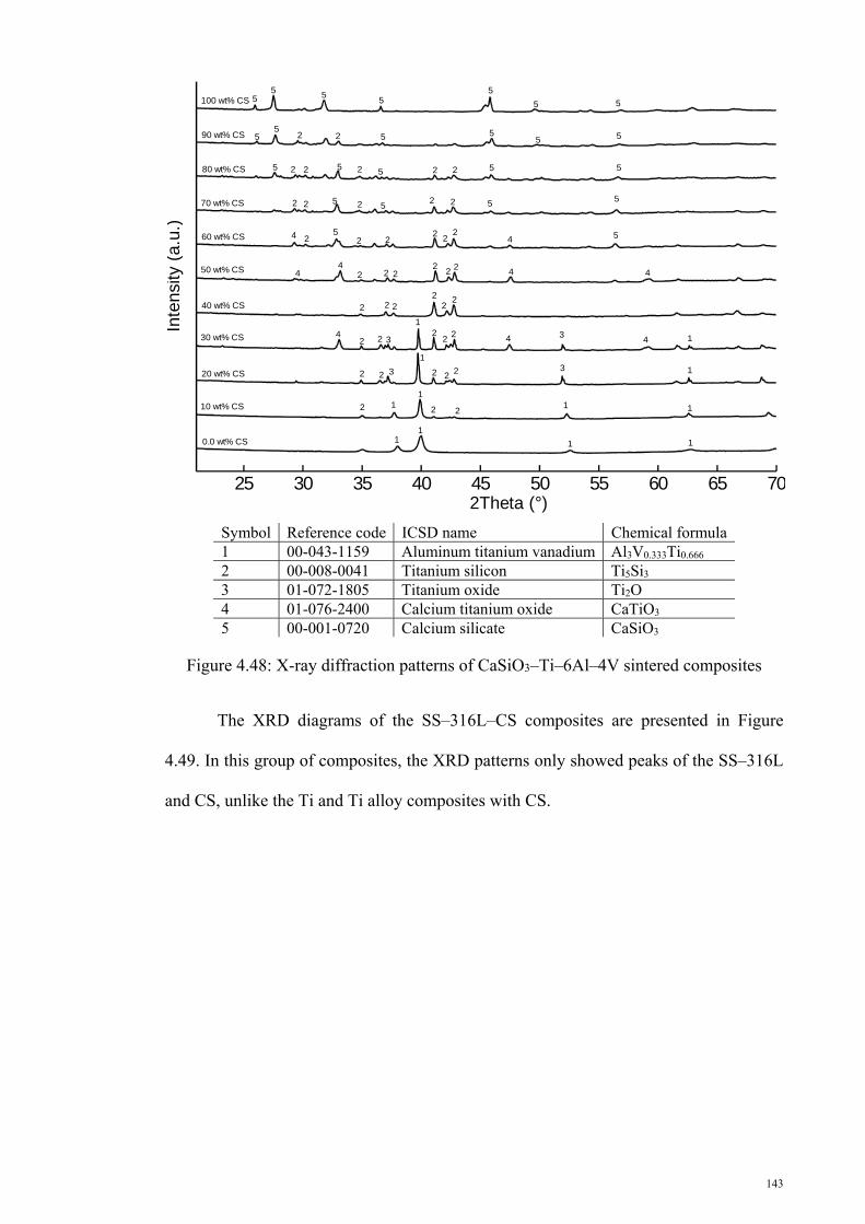
143
Figure 4.48: X-ray diffraction patterns of CaSiO3–Ti–6Al–4V sintered composites
The XRD diagrams of the SS–316L–CS composites are presented in Figure
4.49. In this group of composites, the XRD patterns only showed peaks of the SS–316L
and CS, unlike the Ti and Ti alloy composites with CS.
25 30 35 40 45 50 55 60 65 70
11
1 1
1
1
1
1 1
3
3
1
1
1
2 2 2
222 2 3
322
2
2
22
2
222
22 2
22
22
2
2
2
2
2
2
2
2 2
2 2
2
2
2
2
2
2
2
2
4 4
444
4
4
4
4 55
55
5
55 5
55
5
5
5
55
5
5
5
5
55
55
5
0.0 wt% CS
10 wt% CS
20 wt% CS
30 wt% CS
40 wt% CS
50 wt% CS
60 wt% CS
70 wt% CS
80 wt% CS
90 wt% CS
100 wt% CS
2Theta (°)
Inte
nsity
(a.
u.)
Symbol Reference code ICSD name Chemical formula1 00-043-1159 Aluminum titanium vanadium Al3V0.333Ti0.666 2 00-008-0041 Titanium silicon Ti5Si3 3 01-072-1805 Titanium oxide Ti2O 4 01-076-2400 Calcium titanium oxide CaTiO3 5 00-001-0720 Calcium silicate CaSiO3
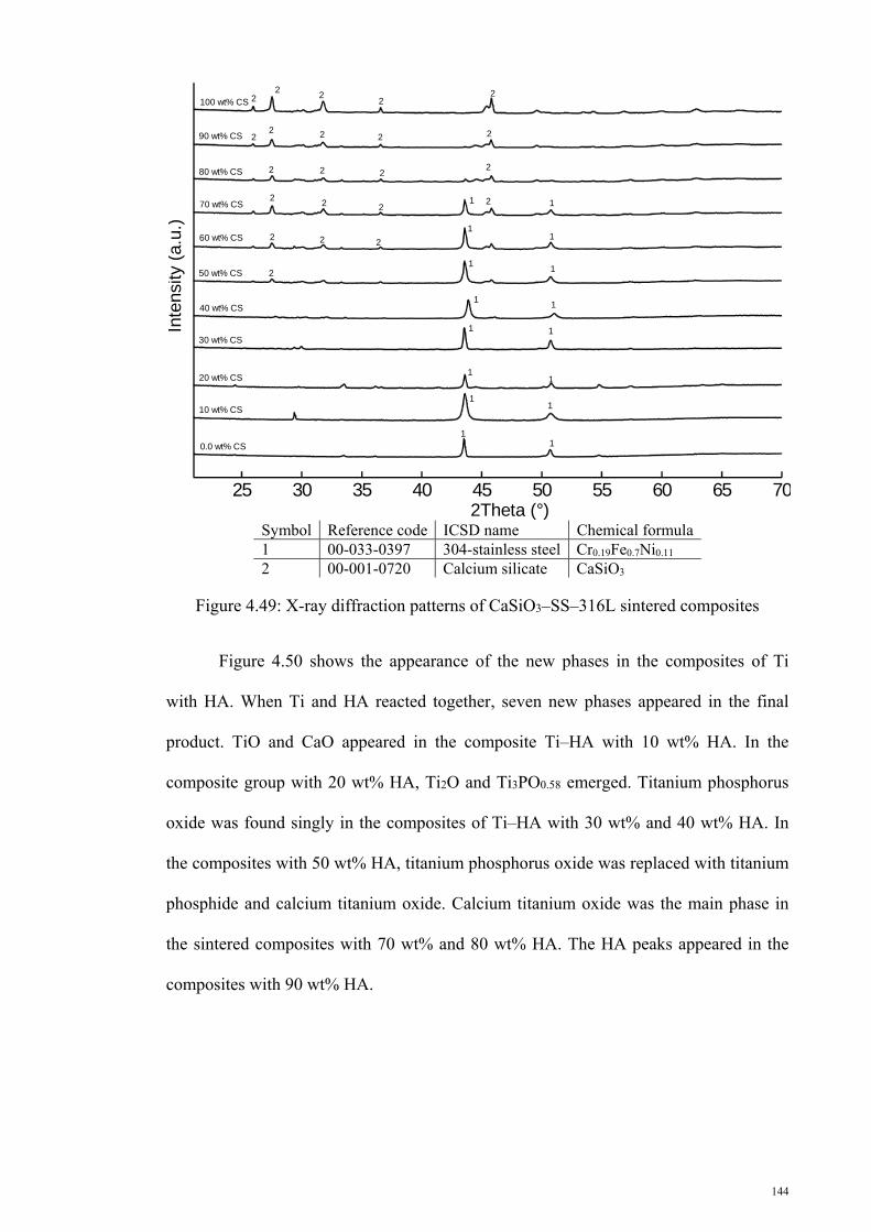
144
Symbol Reference code ICSD name Chemical formula 1 00-033-0397 304-stainless steel Cr0.19Fe0.7Ni0.11 2 00-001-0720 Calcium silicate CaSiO3
Figure 4.49: X-ray diffraction patterns of CaSiO3–SS–316L sintered composites
Figure 4.50 shows the appearance of the new phases in the composites of Ti
with HA. When Ti and HA reacted together, seven new phases appeared in the final
product. TiO and CaO appeared in the composite Ti–HA with 10 wt% HA. In the
composite group with 20 wt% HA, Ti2O and Ti3PO0.58 emerged. Titanium phosphorus
oxide was found singly in the composites of Ti–HA with 30 wt% and 40 wt% HA. In
the composites with 50 wt% HA, titanium phosphorus oxide was replaced with titanium
phosphide and calcium titanium oxide. Calcium titanium oxide was the main phase in
the sintered composites with 70 wt% and 80 wt% HA. The HA peaks appeared in the
composites with 90 wt% HA.
25 30 35 40 45 50 55 60 65 70
0.0 wt% CS
10 wt% CS
20 wt% CS
30 wt% CS
40 wt% CS
50 wt% CS
60 wt% CS
70 wt% CS
80 wt% CS
90 wt% CS
100 wt% CS
2Theta (°)
Inte
nsity
(a.
u.)
11
1
1
1
1
1
1
1
1
1
1
1
1
1
1
22
22
2
2
2
2
22 2 2
2 2 2
22 2
2 2 2
2

145
Symbol Reference code ICSD name Chemical formula 1 00-001-1197 Titanium Ti 2 00-043-1001 Calcium oxide CaO 3 01-086-2352 Titanium oxide TiO 4 01-072-1805 Titanium oxide Ti2O 5 00-050-0247 Titanium phosphate Ti3PO0.58 6 01-087-2178 Titanium phosphorus oxide Ti3PO0.58 7 01-073-1816 Titanium phosphide Ti5P3.16 8 00-042-0423 Calcium titanium oxide CaTiO3 9 00-001-1008 Hydroxyapatite Ca10(OH)2(PO4)6
Figure 4.50: X-ray diffraction patterns of Ca10(OH)2(PO4)6–Ti sintered composites
The XRD patterns of the composites of Ti–6Al–4V–HA are shown in Figure
4.51. Titanium oxide, titanium phosphorus oxide, titanium phosphide, titanium
phosphate, calcium titanium oxide, titanium phosphide, and calcium titanium oxide
were the new phases that appeared during the sintering of the composites of Ti–6Al–4V
with HA. Similar to the Ti–HA composites, the Ti oxides emerged in the Ti-rich
composites, and calcium titanium oxide appeared in the HA-rich composites. Titanium
phosphorus oxide, titanium phosphate, and titanium phosphide appeared in the
composites with 40wt%–60wt% HA.
25 30 35 40 45 50 55 60 65 70
1 1
1 11
99
9 99 9 9 9 9
44 44 4 5 5
9 9 9
8 8 89
100 wt% HA
90 wt% HA
80 wt% HA
70 wt% HA
60 wt% HA
50 wt% HA
40 wt% HA
30 wt% HA
20 wt% HA
10 wt% HA
0.0 wt% HA
8 8 8
88 8
8
7778 8
6666
6
6
6 6
2 333 2
2Theta (°)
Inte
nsity
(a.
u.)
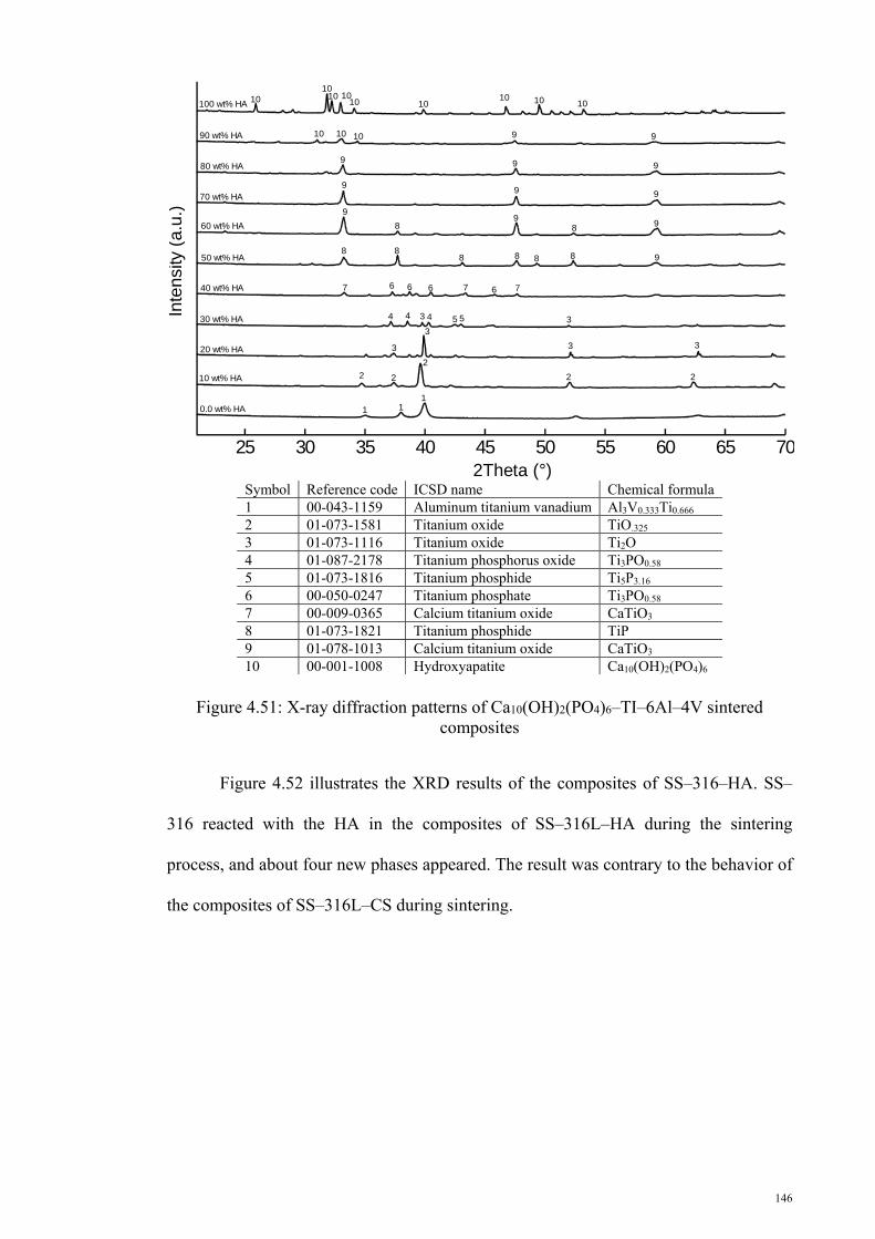
146
Figure 4.51: X-ray diffraction patterns of Ca10(OH)2(PO4)6–TI–6Al–4V sintered composites
Figure 4.52 illustrates the XRD results of the composites of SS–316–HA. SS–
316 reacted with the HA in the composites of SS–316L–HA during the sintering
process, and about four new phases appeared. The result was contrary to the behavior of
the composites of SS–316L–CS during sintering.
25 30 35 40 45 50 55 60 65 70
0.0 wt% HA
10 wt% HA
20 wt% HA
30 wt% HA
40 wt% HA
50 wt% HA
60 wt% HA
70 wt% HA
80 wt% HA
90 wt% HA
100 wt% HA
1 11
2
222 2
3
3 33
5344 54 3
8 88 8 8 98
8 8 99
9
99
9
9 9 9
9 910 1010
1010
10 1010 10 1010 10
6 7667 6 7
2Theta (°)
Inte
nsity
(a.
u.)
Symbol Reference code ICSD name Chemical formula 1 00-043-1159 Aluminum titanium vanadium Al3V0.333Ti0.666 2 01-073-1581 Titanium oxide TiO.325 3 01-073-1116 Titanium oxide Ti2O 4 01-087-2178 Titanium phosphorus oxide Ti3PO0.58 5 01-073-1816 Titanium phosphide Ti5P3.16 6 00-050-0247 Titanium phosphate Ti3PO0.58 7 00-009-0365 Calcium titanium oxide CaTiO3 8 01-073-1821 Titanium phosphide TiP 9 01-078-1013 Calcium titanium oxide CaTiO3 10 00-001-1008 Hydroxyapatite Ca10(OH)2(PO4)6
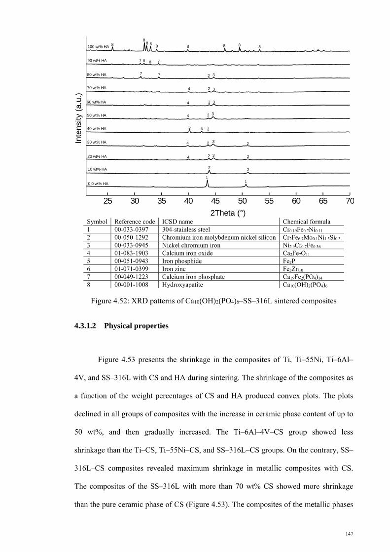
147
Figure 4.52: XRD patterns of Ca10(OH)2(PO4)6–SS–316L sintered composites
4.3.1.2 Physical properties
Figure 4.53 presents the shrinkage in the composites of Ti, Ti–55Ni, Ti–6Al–
4V, and SS–316L with CS and HA during sintering. The shrinkage of the composites as
a function of the weight percentages of CS and HA produced convex plots. The plots
declined in all groups of composites with the increase in ceramic phase content of up to
50 wt%, and then gradually increased. The Ti–6Al–4V–CS group showed less
shrinkage than the Ti–CS, Ti–55Ni–CS, and SS–316L–CS groups. On the contrary, SS–
316L–CS composites revealed maximum shrinkage in metallic composites with CS.
The composites of the SS–316L with more than 70 wt% CS showed more shrinkage
than the pure ceramic phase of CS (Figure 4.53). The composites of the metallic phases
25 30 35 40 45 50 55 60 65 70
77 8 8
88
8 88 8 8 8 8
2Theta (°)
Inte
nsity
(a.
u.)
11
22
22 34
2324
3
3
3
3
2
2
2
2
2
4
4
4
0.0 wt% HA
10 wt% HA
20 wt% HA
30 wt% HA
40 wt% HA
50 wt% HA
60 wt% HA
70 wt% HA
80 wt% HA
90 wt% HA
100 wt% HA
5 6
7 7
Symbol Reference code ICSD name Chemical formula 1 00-033-0397 304-stainless steel Cr0.19Fe0.7Ni0.11 2 00-050-1292 Chromium iron molybdenum nickel silicon Cr2Fe6.7Mo0.1Ni1.3Si0.3 3 00-033-0945 Nickel chromium iron Ni2.9Cr0.7Fe0.36 4 01-083-1903 Calcium iron oxide Ca2Fe7O11 5 00-051-0943 Iron phosphide Fe2P 6 01-071-0399 Iron zinc Fe3Zn10 7 00-049-1223 Calcium iron phosphate Ca19Fe2(PO4)14 8 00-001-1008 Hydroxyapatite Ca10(OH)2(PO4)6
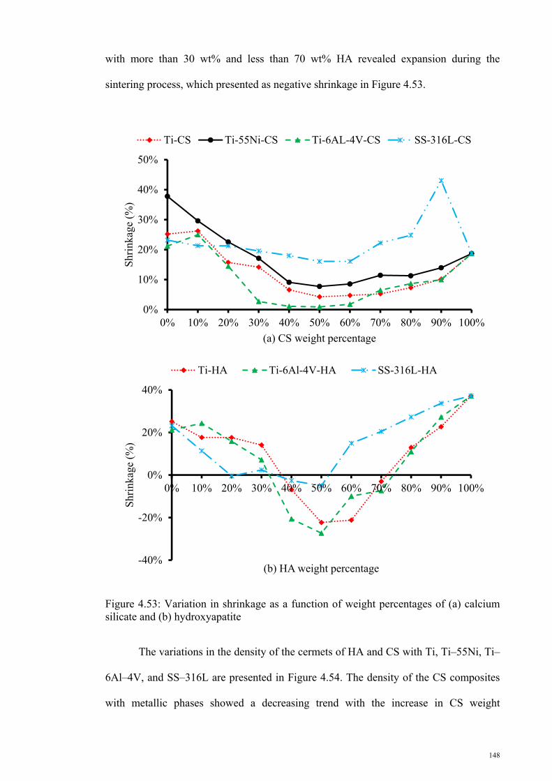
148
with more than 30 wt% and less than 70 wt% HA revealed expansion during the
sintering process, which presented as negative shrinkage in Figure 4.53.
Figure 4.53: Variation in shrinkage as a function of weight percentages of (a) calcium silicate and (b) hydroxyapatite
The variations in the density of the cermets of HA and CS with Ti, Ti–55Ni, Ti–
6Al–4V, and SS–316L are presented in Figure 4.54. The density of the CS composites
with metallic phases showed a decreasing trend with the increase in CS weight
0%
10%
20%
30%
40%
50%
0% 10% 20% 30% 40% 50% 60% 70% 80% 90% 100%
Shr
inka
ge (
%)
(a) CS weight percentage
Ti-CS Ti-55Ni-CS Ti-6AL-4V-CS SS-316L-CS
-40%
-20%
0%
20%
40%
0% 10% 20% 30% 40% 50% 60% 70% 80% 90% 100%
Shr
inka
ge (
%)
(b) HA weight percentage
Ti-HA Ti-6Al-4V-HA SS-316L-HA

149
percentage. Accordingly, the pure metallic phases had maximum density, and the pure
ceramic phases showed minimum density. On the contrary, the composites of HA and
metallic phases produced convex plots with the peak density in the pure phase of metals
and HA, and the groups with expansion showed minimum densities because of the
increase in their volume during sintering.
Figure 4.54: Variation in density as a function of the weight percentages of (a) calcium silicate and (b) hydroxyapatite
0.E+00
2.E-03
4.E-03
6.E-03
8.E-03
0% 10% 20% 30% 40% 50% 60% 70% 80% 90% 100%
Den
sity
(g/
mm
3 )
(a) CS weight percentage
Ti-CS Ti-55Ni-CS Ti-6AL-4V-CS SS-316L-CS
0.E+00
2.E-03
4.E-03
6.E-03
8.E-03
0% 10% 20% 30% 40% 50% 60% 70% 80% 90% 100%
Den
sity
(g/
mm
3 )
(b) HA weight percentage
Ti-HA Ti-6Al-4V-HA SS-316L-HA

150
Figure 4.55a presents the Vickers hardness variation as a function of CS weight
percentage in the composites of CS with metallic phases. The hardness of the CS
composites with Ti alloys exhibited a decreasing trend with the increase in CS content
up to 50wt%, and then their hardness increased gradually at 100wt% CS. On the
contrary, the hardness of the composites of CS with SS–316L enhanced gradually with
the increase in CS content. The composite of SS–316L with 90 wt% CS showed more
hardness than pure CS. Figure 4.55b illustrates the trend of the Vickers hardness
variation as a function of HA weight percentage in the composite metals with HA. The
hardness of Ti alloys with HA decreased with the increase in HA weight percentages up
to 40wt%, and then showed a flat trend between 40wt% and 70 wt% HA. Afterwards,
the hardness enhanced with the increase in HA weight percentage. In SS–316L
composites with HA, the hardness decreased with the increase in HA content up to
40wt%, similar to the Ti alloy composites, and then increased with the increase in HA
weight percentage up to 100%.
0
2
4
6
8
0% 10% 20% 30% 40% 50% 60% 70% 80% 90% 100%
Vic
ker's
har
dnes
s (G
Pa)
(a) CS weight percentage
Ti-CS Ti-55Ni-CS Ti-6AL-4V-CS SS-316L-CS

151
Figure 4.55: Vickers hardness variation as a function of weight percentages of (a) calcium silicate and (b) hydroxyapatite
4.3.1.3 Mechanical properties of the composites
The compressive Young’s modulus of the different composites as a function of
the weight percentages CS and HA are tabulated in Tables 4.5 and 4.6, respectively. The
compressive Young’s modulus decreased with the increase in ceramic phases up to
around 50wt%. Afterward, the Young’s modulus gradually increased with the ceramic
phase content. The CS composite groups showed higher values of Young’s modulus
than the HA composite groups.
0
1
2
3
4
5
6
0% 10% 20% 30% 40% 50% 60% 70% 80% 90% 100%
Vic
ker's
har
dnes
s (G
Pa)
(b) HA weight percentage
Ti-HA Ti-6Al-4V-HA SS-316L-HA

152
Table 4.5: Variation in Young’s modulus as a function of calcium silicate weight percentage
E (GPa) ± STD (GPa) Material Ti Ti–55Ni Ti–6Al–4V SS–316L
CS (wt.%) E STD E STD E STD E STD 0 120.4 3.9 112.1 27.7 131.7 6.0 213.8 13.3
10 88.3 5.9 103.9 17.4 84.2 6.0 127.0 2.3 20 72.3 9.6 85.9 8.0 84.5 8.4 121.7 12.8 30 89.7 13.4 81.2 9.0 62.4 1.5 85.4 2.2 40 63.5 4.7 77.3 8.8 39.6 7.2 81.5 10.0 50 64.1 4.3 82.7 26.5 59.7 4.2 78.6 21.4 60 80.3 4.9 88.9 10.0 70.2 3.2 90.6 4.2 70 87.3 11.9 107.9 63.3 78.1 6.2 99.7 4.6 80 97.4 2.6 106.7 6.2 89.2 7.1 115.0 17.0 90 102.1 8.7 108.2 9.6 95.7 2.0 119.4 12.5
100 106.9 24.8 106.9 24.8 106.9 24.8 106.9 24.8
Table 4.6: Young’s modulus variation as a function of hydroxyapatite weight percentage
E (GPa) ± STD (GPa) Material Ti Ti–6Al–4V SS–316L
HA (wt.%) E STD E STD E STD 0 120.4 3.9 131.7 6.0 213.8 13.3 10 117.3 1.6 108.8 5.7 132.3 15.9 20 108.1 3.5 107.1 10.6 41.9 4.5 30 95.7 7.0 98.6 3.5 58.6 5.9 40 35.0 1.4 39.6 2.8 51.2 3.3 50 56.2 4.5 27.3 4.4 82.0 2.8 60 24.4 6.7 24.1 2.1 118.2 8.0 70 13.3 5.5 10.9 5.5 128.4 3.2 80 17.3 3.1 28.1 2.1 128.4 7.9 90 73.6 4.6 83.4 1.5 89.2 19.1
100 56.3 6.1 56.3 6.1 56.3 6.1
The ultimate compressive strengths of the composite metallic phases with
different CS and HA contents are presented in Tables 4.7 and 4.8, respectively. Similar
to the Young’s modulus, the ultimate compressive strength of the composites declined
with the increase in the contents of ceramic phases up to 50wt%. Afterward, the
ultimate compressive strength of the composites increased along with the ceramic phase
contents. The CS composites with SS–316L showed better performance than the
composites of Ti alloys with CS. On the contrary, in the HA composite groups, the
composites of the Ti alloys with HA showed better performance compared with the
composites of the SS–316L with HA.
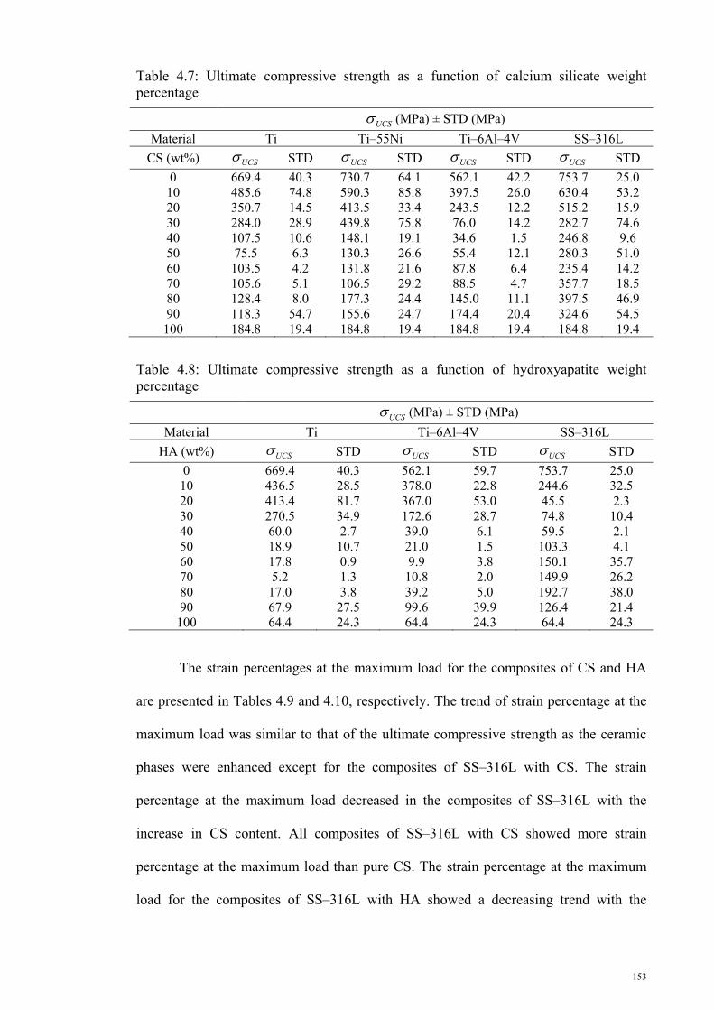
153
Table 4.7: Ultimate compressive strength as a function of calcium silicate weight percentage
UCS (MPa) ± STD (MPa)
Material Ti Ti–55Ni Ti–6Al–4V SS–316L
CS (wt%) UCS STD UCS STD UCS STD UCS STD
0 669.4 40.3 730.7 64.1 562.1 42.2 753.7 25.0 10 485.6 74.8 590.3 85.8 397.5 26.0 630.4 53.2 20 350.7 14.5 413.5 33.4 243.5 12.2 515.2 15.9 30 284.0 28.9 439.8 75.8 76.0 14.2 282.7 74.6 40 107.5 10.6 148.1 19.1 34.6 1.5 246.8 9.6 50 75.5 6.3 130.3 26.6 55.4 12.1 280.3 51.0 60 103.5 4.2 131.8 21.6 87.8 6.4 235.4 14.2 70 105.6 5.1 106.5 29.2 88.5 4.7 357.7 18.5 80 128.4 8.0 177.3 24.4 145.0 11.1 397.5 46.9 90 118.3 54.7 155.6 24.7 174.4 20.4 324.6 54.5
100 184.8 19.4 184.8 19.4 184.8 19.4 184.8 19.4
Table 4.8: Ultimate compressive strength as a function of hydroxyapatite weight percentage
UCS (MPa) ± STD (MPa)
Material Ti Ti–6Al–4V SS–316L
HA (wt%) UCS STD UCS STD UCS STD
0 669.4 40.3 562.1 59.7 753.7 25.0 10 436.5 28.5 378.0 22.8 244.6 32.5 20 413.4 81.7 367.0 53.0 45.5 2.3 30 270.5 34.9 172.6 28.7 74.8 10.4 40 60.0 2.7 39.0 6.1 59.5 2.1 50 18.9 10.7 21.0 1.5 103.3 4.1 60 17.8 0.9 9.9 3.8 150.1 35.7 70 5.2 1.3 10.8 2.0 149.9 26.2 80 17.0 3.8 39.2 5.0 192.7 38.0 90 67.9 27.5 99.6 39.9 126.4 21.4
100 64.4 24.3 64.4 24.3 64.4 24.3
The strain percentages at the maximum load for the composites of CS and HA
are presented in Tables 4.9 and 4.10, respectively. The trend of strain percentage at the
maximum load was similar to that of the ultimate compressive strength as the ceramic
phases were enhanced except for the composites of SS–316L with CS. The strain
percentage at the maximum load decreased in the composites of SS–316L with the
increase in CS content. All composites of SS–316L with CS showed more strain
percentage at the maximum load than pure CS. The strain percentage at the maximum
load for the composites of SS–316L with HA showed a decreasing trend with the

154
increase in HA content up to 50 wt% HA, and then gradually increased with the
increase in HA wt%.
Table 4.9: Strain percentage at maximum load as a function of calcium silicate weight percentage
ε (%) ± STD (%) Material Ti Ti–55Ni Ti–6Al–4V SS–316L
CS (wt%) ε STD ε STD ε STD ε STD 0 3.9 0.6 4.4 0.5 5.0 0.4 14.8 0.4 10 3.1 0.3 4.5 0.5 3.9 2.0 14.0 0.2 20 2.8 0.3 3.9 0.7 2.7 0.1 11.7 0.9 30 2.2 0.2 3.1 0.6 2.9 0.4 4.5 0.6 40 2.2 0.7 1.7 0.1 1.3 0.0 3.5 0.3 50 2.3 0.2 1.5 0.2 1.6 0.6 3.6 0.2 60 1.8 0.4 1.6 0.0 1.5 0.0 3.0 0.8 70 1.4 0.3 1.3 0.4 1.6 0.2 3.0 0.5 80 1.7 0.2 2.1 0.3 2.2 0.8 2.4 0.3 90 1.7 0.2 1.4 0.2 2.4 0.1 2.2 1.1
100 1.8 0.7 1.8 0.7 1.8 0.7 1.8 0.7
Table 4.10: Strain percentage at maximum load as a function of hydroxyapatite weight percentage
ε (%) ± STD (%) Material Ti Ti–6Al–4V SS–316L
HA (wt%) ε STD ε% STD ε STD 0 3.9 0.6 5.0 0.4 14.8 0.4 10 3.3 0.5 4.3 0.2 11.7 1.4 20 3.0 0.6 3.6 0.4 3.3 0.2 30 2.8 0.4 3.4 0.4 2.1 0.6 40 2.4 0.4 2.2 0.1 1.7 0.2 50 0.7 0.6 1.4 0.3 1.8 0.3 60 1.4 0.2 1.5 1.1 1.9 0.5 70 1.1 0.7 2.2 0.8 1.5 0.4 80 1.7 0.5 2.7 0.4 2.4 0.8 90 2.1 1.1 3.4 0.9 2.5 0.8
100 3.7 0.9 3.7 0.9 3.7 0.9
4.3.2 Functionally graded materials
4.3.2.1 Physical properties
The physical properties [shrinkage (%) and density (ρ)] of the FGMs
composed of CS and HA with Ti, Ti–6AL–4V, Ti–55Ni, and SS–316L are presented in
Tables 4.11 to 4.12. The FGMs were sintered at 1000 °C, 1100 °C, and 1200 °C. The
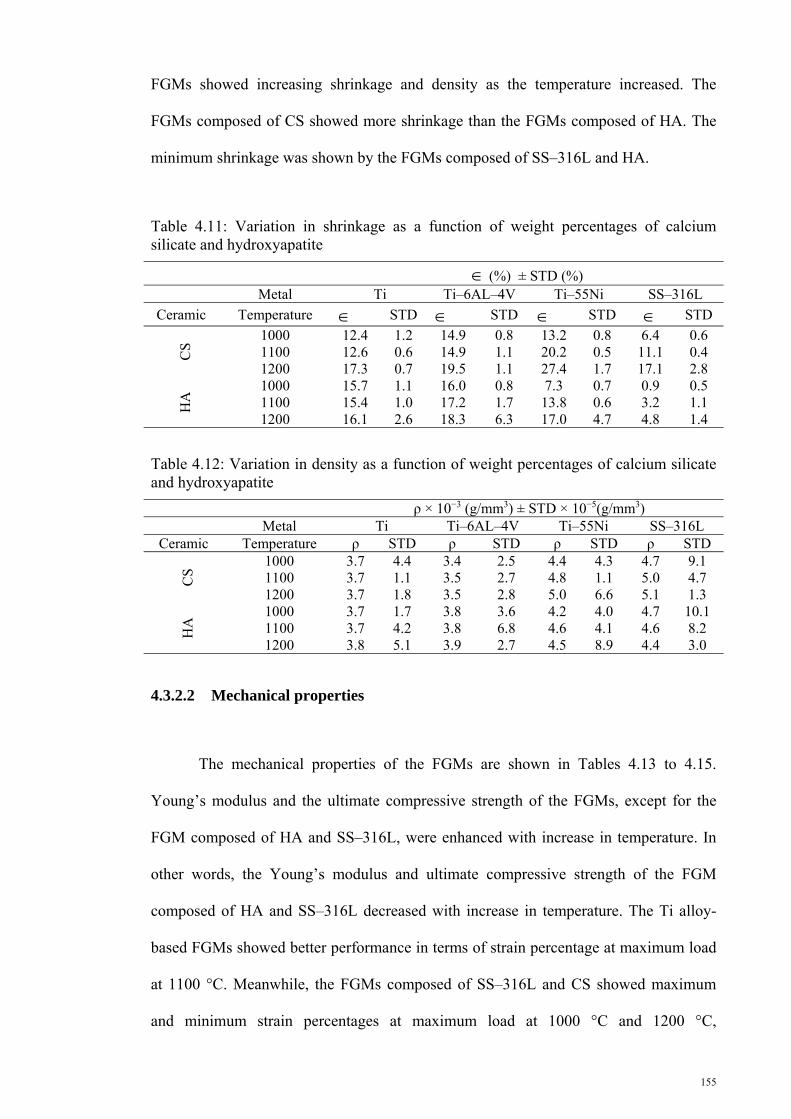
155
FGMs showed increasing shrinkage and density as the temperature increased. The
FGMs composed of CS showed more shrinkage than the FGMs composed of HA. The
minimum shrinkage was shown by the FGMs composed of SS–316L and HA.
Table 4.11: Variation in shrinkage as a function of weight percentages of calcium silicate and hydroxyapatite
(%) ± STD (%) Metal Ti Ti–6AL–4V Ti–55Ni SS–316L
Ceramic Temperature STD STD STD STD
CS
1000 12.4 1.2 14.9 0.8 13.2 0.8 6.4 0.6 1100 12.6 0.6 14.9 1.1 20.2 0.5 11.1 0.4 1200 17.3 0.7 19.5 1.1 27.4 1.7 17.1 2.8
HA
1000 15.7 1.1 16.0 0.8 7.3 0.7 0.9 0.5 1100 15.4 1.0 17.2 1.7 13.8 0.6 3.2 1.1 1200 16.1 2.6 18.3 6.3 17.0 4.7 4.8 1.4
Table 4.12: Variation in density as a function of weight percentages of calcium silicate and hydroxyapatite
ρ × 10−3 (g/mm3) ± STD × 10−5(g/mm3) Metal Ti Ti–6AL–4V Ti–55Ni SS–316L
Ceramic Temperature ρ STD ρ STD ρ STD ρ STD
CS
1000 3.7 4.4 3.4 2.5 4.4 4.3 4.7 9.1 1100 3.7 1.1 3.5 2.7 4.8 1.1 5.0 4.7 1200 3.7 1.8 3.5 2.8 5.0 6.6 5.1 1.3
HA
1000 3.7 1.7 3.8 3.6 4.2 4.0 4.7 10.1 1100 3.7 4.2 3.8 6.8 4.6 4.1 4.6 8.2 1200 3.8 5.1 3.9 2.7 4.5 8.9 4.4 3.0
4.3.2.2 Mechanical properties
The mechanical properties of the FGMs are shown in Tables 4.13 to 4.15.
Young’s modulus and the ultimate compressive strength of the FGMs, except for the
FGM composed of HA and SS–316L, were enhanced with increase in temperature. In
other words, the Young’s modulus and ultimate compressive strength of the FGM
composed of HA and SS–316L decreased with increase in temperature. The Ti alloy-
based FGMs showed better performance in terms of strain percentage at maximum load
at 1100 °C. Meanwhile, the FGMs composed of SS–316L and CS showed maximum
and minimum strain percentages at maximum load at 1000 °C and 1200 °C,

156
respectively. On the contrary, the strain percentage at maximum load decreased in the
FGMs composed of SS–316L and HA with the increase in temperature.
Table 4.13: Compressive Young’s modulus as a function of weight percentages of calcium silicate and hydroxyapatite
E (GPa) ± STD (GPa) Metal Ti Ti–6AL–4V Ti–55Ni SS–316L
Ceramic Temperature E STD E STD E STD E STD
CS
1000 106.9 37.7 67.7 12.8 108.7 17.33 110.8 7.4 1100 119.3 15.3 61.8 5.6 110.9 10.60 143.4 18.0 1200 144.4 28.8 103.0 12.1 143.3 20.92 187.4 35.0
HA
1000 104.4 15.3 94.2 18.0 118.1 8.58 94.3 6.7 1100 114.2 8.4 102.5 45.2 137.9 3.37 85.4 16.3 1200 129.9 45.0 113.8 7.4 139.4 14.37 74.7 8.2
Table 4.14: Ultimate compressive strength as a function of weight percentages of calcium silicate and hydroxyapatite
UCS (MPa) ± STD (MPa)
Metal Ti Ti–6AL–4V Ti–55Ni SS–316L
Ceramic Temperature UCS STD UCS STD UCS STD UCS STD
CS
1000 130.3 10.7 69.7 9.6 187.4 16.6 175.8 46.3 1100 134.4 9.1 59.0 2.9 190.7 8.6 206.4 28.8 1200 170.9 78.2 86.9 12.0 349.6 22.1 347.3 20.6
HA
1000 96.6 14.0 165.4 33.9 169.2 21.9 168.4 29.6 1100 101.9 11.4 125.5 7.2 183.2 20.6 76.9 20.6 1200 178.3 45.8 145.9 24.3 228.3 50.6 75.3 3.1
Table 4.15: Compressive strain percentage at maximum load as a function of weight percentages of calcium silicate and hydroxyapatite
ε (%) ± STD (%) Metal Ti Ti–6AL–4V Ti–55Ni SS–316L
Ceramic Temperature ε STD ε STD ε STD ε STD
CS
1000 4.1 0.5 3.3 0.4 3.6 0.9 4.8 1.4 1100 4.7 1.0 3.5 0.0 3.2 0.4 5.6 2.1 1200 3.3 0.6 2.6 1.0 5.9 1.0 6.1 1.5
HA
1000 3.1 1.2 3.4 0.7 3.4 0.1 5.6 0.5 1100 4.8 1.5 3.7 0.2 3.7 0.4 3.2 0.9 1200 3.3 0.5 5.4 0.1 3.3 0.8 3.4 0.4

157
CHAPTER 5
5. DISCUSSION
5.1 Introduction
This chapter discusses the inferences from FEA and experimental results
presented in the previous chapter. It is commenced with the discussion on the FEA
results on the utilization of FGMs in prostheses. The presence of circumferential cracks
in the cement layer is then discussed. Finally, the chapter is ended by a discussion about
the experimental results.
5.2 Finite element analysis on the utilization of functionally graded material in femoral prosthesis design
The selection of materials for use in prosthesis is complex because the introduction
of any implant to the aggressive physiological environment of the human body results in
various biological and mechanical stresses (Enab & Bondok, 2013). The implant
material must be biocompatible and resistant to corrosion and wear (Janssen et al.,
2008). Moreover, the Young’s modulus of prosthesis material directly affects prosthesis
stiffness, stress shielding, and interface stresses. The Young’s modulus of the most
conventional materials (Ti alloy, Cr–Co, and St alloy) applied in femoral prosthesis is
higher than that of the cortical bone, which leads to a risk of THR failure because of
stress shielding. Therefore, the ability to design and manufacture a prosthesis that can
incorporate bespoke and adjustable stiffness is one of the main objectives in prosthesis
design (Taylor et al., 2013). This feature allows prosthetists to match the prosthesis and
bone stiffness. Changes in the designs and materials used in the construction of the
prostheses present the two possible methods to achieve this goal.

158
In the FGM-based prostheses, the increase in gradient index dictates an increase in
the volume fraction of the phase with low Young’s modulus. Consequently, the
Young’s modulus of FG prosthesis decreases in the gradient direction in both sagittal
and transverse planes with gradient index growth. This condition leads to the reduction
in the stiffness of prostheses regardless of gradient direction. Therefore, more SED are
induced to the bone because of the adverse relationship between the stiffness of
prosthesis and the stimulated SED to the proximal metaphysis of femur. This incident is
also reported by Yildiz et al. (1998), and they showed more SED in the bone for Ti-
based prosthesis than St-based prosthesis. In the present study, the Ti-based prostheses
caused 31.0% and 27.3% more SED in the bone than the St-based prostheses in the
cemented and cementless prostheses, respectively. The FG prostheses with gradient
index of 1 produced more SED regardless of prostheses type (RP or LP) and geometry.
Meanwhile, Simões and Marques (2005) showed an increase in the SED for LP
prosthesis composed of carbon fiber with a metal core. Their finding was generally
consistent with the findings in the current study. The SED increased by approximately
20.2% in cementless LP, 32.6% in cementless RP, 21.3% in cemented LP, and 27.8% in
cemented RP for the increase in gradient index from 0 to 1. The SED also showed
dependence on prostheses geometry because the rigidity of prosthesis is also a function
of the prosthesis cross-section geometry. The distal cross-sections showed less effect on
the SED variation compared with the proximal cross-sections based on the measurement
of SED at the proximal and spongy portion of the femur. The average difference in the
SED caused by the implantation of the prostheses with different distal cross-sections
was about 6.3%, whereas proximal cross-sections provoked a difference of about 9.4%
and 21.4% for cemented and cementless prostheses, respectively. Altering the profiles
of the prostheses changed the SED by approximately 1.3% and 17.6% in the cemented

159
and cementless prostheses, respectively. The effect of the interface property on SED for
cementless LP was negligible at about 0.6%.
The increase in gradient index as previously mentioned leads to the reduction in
prosthesis stiffness and the mismatch between bone and prostheses stiffness. Therefore,
loads distribute more equally between the constituents of the THR. Prostheses with
lower stiffness carry less stress than stiffer prostheses. This phenomenon was
demonstrated by El-Sheikh et al. (2002) and is also compatible with the findings of the
present work for St and Ti. In FG prostheses, the developed stress in the cementless RP
showed maximum reduction of 79.1% when gradient index increased from 0 to 1, and
the minimum decrease in the developed stress to the prostheses was revealed in the
cemented LP prostheses at about 26.3%. The stresses in the cementless LP and
cemented RP declined by about 31.9% and 54.3%, respectively. This reduction in the
stress in the femoral prostheses for FG prostheses was in agreement with the findings of
Simões and Marques (2005) for LP. The developed stress in the implant is also a
function of prostheses geometry specifications. Among the prostheses specifications,
the profile exhibited minor effect on stress variation, but the proximal cross-section
showed maximum influence on stress distribution. The average variations in stress
caused by the change in the distal cross-sections, proximal cross-sections, and profiles
were 10.3%, 15.9%, and 3.4%, respectively.
Loads transfer to the bone mainly from the proximal portion of the prosthesis in
low-stiffness prostheses, nearly the whole length of prosthesis in moderate-stiffness
prostheses, and distal part of prosthesis in highly stiff prosthesis (Pyburn & Goswami,
2004). Meanwhile, bone is a live tissue that adapts to its biological and mechanical
environment. The alteration in load transfer and removal of a portion of the load caused
by inserting an implant lead to changes in bone structures and strength. Therefore, an

160
implant should as much as possible mimic the natural loading condition of the hip joint
without exposing the bone to too much stress. In addition, the maximum stress criterion
can predict bone failure showing <30% error (Doblaré et al., 2004). The increase in
gradient index as previously noted reduces the mismatch between prosthesis and bone,
and more loads transfer to the bone. Consequently, both maximum and minimum
principal stresses increases with the gradient index. This observation indicates that more
load transfer to the proximal portion of the femur and subsequently leads to less stress
shielding in the bone, whereas the developed stresses to the bone caused by the increase
in loads are much less than the ultimate tensile strength (121 MPa) and ultimate
compressive strength (167 MPa) of the bone. The gradient index contributes more to the
change in the developed stress in the bone in the cementless prostheses than in the
cemented prostheses. In addition, the stress distribution in the bone is also a function of
prosthesis geometry. The geometry of prosthesis was more influential on the developed
stress in the bone in the cemented prostheses than the cementless prostheses. The distal
cross-sections showed greater contribution in the change in stresses than the proximal
cross-section and profile, the effects of which on the developed stress in the bone were
almost similar.
Load transfer to the bone in the cemented fixation method occurs through the
cement layer, which also provides stability and fixation of the cemented prostheses
within the host bone. Therefore, overstressing the cement layer leads to the failure of the
cement layer, loosening of the stem, and ultimately THR failure. Mechanical failure is
the main reason for cement failure (James et al., 1992). Given that orthopedic cement is
a brittle material, it is weaker under tensile loads than at compressive loads. Loads
transfer through the prosthesis to the cement and then to the bone. Therefore, the main
portion of the loads are applied to the internal surface of the cement, and then moved to
the external surface. Hence, the internal surface of the cement layer carried more
161
maximum and minimum principal stresses in both LP and RP. The maximum principal
stress at the lateral side and the minimum principal stress at the medial side of the
cement layer showed two different trends with the increase in gradient index. In other
words, the maximum principal stress increased with the increase in gradient index,
contrary to the decreasing trend of the minimum principal stress under the same
condition. The developed stresses in the cement layer showed sensitivity to the
geometry of prostheses, which is consistent with the findings of Ramos et al. (2012).
The prostheses with D3 distal cross-section and P3 proximal cross-section induced the
lowest values of the maximum and minimum principal stress.
The interface stresses have a significant role on the initial stability of the prostheses
and the long term survival of THR, especially for cementless prostheses. The geometry
and gradient index high influence the interface stresses. The interface stresses at the
implant–bone interface decreased with the increase in gradient index, which is not
consistent with those in prostheses composed of conventional materials. In other words,
the interface stresses at the implant–bone interface declined with the increasing Young’s
modulus of the conventional materials applied in the prosthesis, whereas their stress
shielding effect increased (Simões & Marques, 2005). The results in the present study
are supported by the findings of Hedia et al. (2004; 2006). The effect of geometrical
specification on the interface stresses is consistent with the statements of Pal et al.
(2013) with regard to the effect of geometric features on the stability of hip stem.
Meanwhile, in RP, the prosthesis with D3 distal cross-section, P4 proximal cross-
section, and Profile 1 induced minimum interface stresses, whereas in LP, the minimum
interface stress was provoked by the prosthesis with D4 distal cross-section, P3
proximal cross-section, and Profile 3.

162
5.3 Existence of circumferential crack in the cement layer
Orthopedic cement is categorized as a brittle material (Culleton et al., 1993;
McCormack et al., 1999; Topoleski et al., 1998), and SIFs are valid and applicable for
the analysis of the crack behavior inside the cement. Accordingly, by understanding the
SIFs during the different stages of walking, the lifespan of the cement layer and the
crack growth rate in a gait cycle can be predicted using crack propagation laws such as
Paris’ law. Crack initiation and propagation at the cement–prosthesis or cement–bone
interfaces present a contradictory discussion. Several researchers believe that cracks
initiate and propagate from the cement–prosthesis interface, while other researchers
noted that crack initiation and propagation occur in the cement–bone interface (Moreo
et al., 2006; Ramos & Simões, 2009). However, any improvement in the bonding
properties of the cement–bone interface increases the stresses in the interface (Achour et
al., 2010), which explains the high SIFs at the cement–bone interface.
Internal and external cracks do not indicate significant interaction. The
numerical study on the circumferential crack behavior revealed that KII is smaller than
KI and KIII. This behavior is in agreement with the crack geometry effect on the SIFs
explored by Shahani and Habibi (2007). In addition, higher SIF values were obtained at
the distal part compared with the proximal part of the cement layer because post-THR
loads transfer via shear forces across the material interfaces at the proximal to the distal
ends of the stem (Gross & Abel, 2001). Thus, excessive loads were transferred from the
distal area of the prosthesis to the bone through the cement (Ramos et al., 2012) because
of the mismatch between the stiffness of THR components (prosthesis, cement, and
bone). The results of the current study are also supported by the findings of Afsharpoya
et al. (2009) about Charnley prosthesis, in which the peak stresses were concentrated at
the distal end of the prosthesis–cement interface. Such transfer causes extreme stresses

163
at the distal end of the cement layer, thereby enhancing the KI, KII, and KIII values. This
behavior has been proven by Flitti et al. (2010) and Jeffers et al. (2007). The results of
the present study also indicated that SIFs vary along the crack front in the hoop
direction, which correspond to the stress variations in the hoop path reported by
McCormack and Prendergast (1999).
Furthermore, KI and KIII displayed opposite trends in the hoop direction. KI
declined along the lateral and medial to the anterior and posterior directions, whereas
KIII decreased along the anterior and posterior to the lateral and medial directions.
Accordingly, at the crack front, the absolute maximum and minimum values of KI
coincided with the absolute minimum and maximum values of KIII. The crack
propagation was mostly subjected to the combination of both opening and tearing
except at areas with maximum KI or KIII values. The cement corners were under the
highest SIFs on the lateral and medial sides. Subsequently, the risk of crack initiation
and propagation increased at the distal corners of the cement layer, which is consistent
with results from previous studies (Jasty et al., 1991; Verdonschot & Huiskes, 1997).
Finally, the cement layer must withstand the cyclic load during walking. In the
gait cycle, the SIFs attained maximum values in the single-leg stance and push off
phases and then declined to the minimum values during the swing phase. Accordingly,
the cement layer suffered a fatigue load because of the SIF fluctuations, resulting in
crack propagation and cement failure in THR for an extended period (Hung et al.,
2004). Given that the lateral side has to endure regular tensile stress, the risk of a fatigue
crack propagation in this side is greater than that in the medial side. This result
corresponds with the finding of Jeffers et al. (2007). However, both normal and tear
fatigue cracks may occur at the anterior and posterior sides of the cement layer.

164
5.4 Composites and functionally graded materials
Different composites of CS and HA with Ti, Ti–6Al–4V, Ti–55Ni, and SS–
316L were produced and then physically and mechanically tested. Sintering at high
temperature led to the appearance of new phases of materials. The weight ratio of the
raw powders in the mixture showed high impact on the emergence of the new phases.
The appearance of the new phases of the materials demonstrated by (Arifin et al., 2014)
are consistent with findings of the present work. These phases significantly affect the
physical and mechanical properties of the sintered composite materials. Metal or
ceramic-rich composites showed better mechanical performance and hardness than the
composites with 40wt% to 60 wt% metal or ceramic. The trend of hardness in the
present study for the composites of Ti–HA and SS–316L–HA was in agreement with
the demonstrated results in the studies of Chenglin (1999) and Younesi and
Bahrololoom (2010), respectively. Meanwhile, the metal-rich composites carried more
load than the ceramic-rich composites. The composites of CS with SS–316L showed
better mechanical performance compared with the CS composites with Ti and Ti alloys.
The CS composites with SS–316L exhibited more plastic deformation than pure CS by
showing more strain percentage at the maximum load. Meanwhile, the increased
hardness of these composites could help them to resist wear compared with pure SS–
316L (Younesi & Bahrololoom, 2010). On the contrary, the composites of SS–316L
with HA in the metal-rich group showed weak mechanical properties, whereas the
ceramic-rich group exhibited good mechanical performance. The Ti and Ti alloy
composites with HA and CS had almost similar mechanical performance.
FGMs were developed from metal-rich composites because these composites
showed better mechanical performance. Therefore, the FGM layer was composed of
pure metal and the composite with 90 wt%, 80wt%, and 70wt% metal phases and

165
sintered at 1000 °C, 1100 °C, and 1200 °C. The increase in temperature positively
affected the mechanical performance of the FGMs, except for the FGMs composed of
SS–316L and HA, because of the increase in the rate of reaction between SS–316L and
HA. The FGMs showed better properties for hard tissue substitution compared with the
pure materials and single-layer composites. The Young’s modulus of the FGMs was
less than that of pure metals, and their ultimate compressive strength was more than
those of the single-layer composites with CS or HA content ≥30 wt%. Meanwhile, the
FGMs showed more strain at the maximum load and more plasticity and less brittle
properties compared with the single layer of the composites, except for SS–316L
composites with contents of HA or CS and SS–316L ≥ 20wt%.

166
CHAPTER 6
6. CONCLUSION AND RECOMMENDATIONS
6.1 Conclusions
The material and the gradient index are the most influential factors that control
SED in LP and RP. The increase in gradient index resulted in increased SED to the
bone. The geometrical parameters were more influential in the cementless prostheses
than in the cemented prostheses. The cementless RP provoked more SED in the bone
compared with the LP.
The gradient index and geometry are the key factors in changing the developed
stress in the prostheses. However, the influence of the material and gradient index were
greater than that of the geometry of prostheses on the developed stress in the prostheses.
The induced stress to the prostheses decreased with the increase in gradient index.
Profiles showed less effect on the induced stress to the prostheses compared with the
proximal and distal cross-sections. Meanwhile, the cementless prostheses carried less
stress than the cemented prostheses.
The gradient index and geometric parameters are important factors in controlling
and adjusting the developed stress in the bone. The effect of gradient index was more
significant in the cementless prostheses, and the geometric factors were more influential
in the cemented prostheses.
The increase in gradient index showed bilateral effect on the developed stress in
the cement layer. The maximum and minimum principal stresses showed increasing and

167
decreasing trends with the increase in gradient index, respectively. The prostheses made
of distal cross-section D3 and proximal cross-section P3 developed minimum stress in
the cement layer. The effect of the profile depended on the prosthesis type.
The gradient index and geometry highly affected the interface stresses. The
utilization of FGMs and the increasing gradient index led to the decrease in the interface
stress. The geometry should be designed based on prostheses type (RP or LP) to achieve
minimum interface stresses. The RP with distal cross-section D3, proximal cross-
section P4, and Profile 1 induced minimum interface stress, whereas the LP with distal
cross-section D4, proximal cross-section P3, and Profile 3 provoked the minimum
interface stress.
The SIFs were enhanced along the cement from the proximal to the distal end. In
a certain cross section, the SIFs attained a maximum value in the push off and single-leg
stance phases, whereas minimum SIF values were attained in the swing phase of a gait.
KI and KIII were the most superior SIF modes in the cement layer with internal
circumferential cracks. By contrast, KII was approximately a tenth of KI. The KI domain
was at the lateral and medial sides of the cement layer, whereas the KIII domain was at
the anterior and posterior sides. Consequently, the circumferential cracks endured a
normal fatigue at the lateral and medial sides of the cement layer, whereas the anterior
and posterior sides of the cement layer were subjected to a torsional fatigue. Moreover,
the circumferential cracks were propelled by a mixed mode of opening and tearing loads
at a large portion of the crack front. Cracks at the internal and external surfaces of the
cement layer did not show any significant interaction.
The FGMs could be utilized in implants as a proper substitute to conventional
materials because of their unique properties. The FGMs composed of CS and HA with

168
Ti, Ti–6Al–4V, Ti–55Ni, and SS–316L showed lower Young’s moduli than the pure
metals and higher ultimate compressive strength compared with the pure ceramic and
composites with 30 wt% ceramic. In addition, the FGMs showed more plasticity by
exhibiting higher strain percentage at the maximum load compared with the pure
ceramic and composites with more than 30 wt% ceramic.
6.2 Recommendations
The following studies are recommended to improve the performance of the FG
prostheses and prolong the lifespan of the THR, understand the crack behavior and
crack propagation in the cement layer of THR during daily activities, and develop an
MCC, CMC, or FGM with the best performance for the FG prostheses.
The geometry of the prosthesis should be optimized based on a defined gradient
direction (radial or longitudinal). Failure criteria should be embedded to a 3D FEA, and
the risk of failure in the components of the THR with an FG prosthesis should be
assessed. Meanwhile, the adaptation of the bone caused by the impact of the FGMs in
prosthesis should be also examined.
Different cracks should be inserted into the cement layer and evaluated during
main daily activities such as normal walking and stair climbing. In addition, the fatigue
crack propagation should also be considered in the studies to assess the crack
propagation mechanism during different activities.
The composite of metal and ceramic should be optimized in terms of the
material, volume fraction of each phase, sintering temperature, and sintering process to
achieve a composite or FGM with the best mechanical properties for prosthesis.

169
Finally, a prototype of the prosthesis composed of the optimized geometry and
material should be prepared for final assessment and in vitro test.

170
References
Abdul-Kadir, M. R., Hansen, U., Klabunde, R., Lucas, D., & Amis, A. (2008). Finite element modelling of primary hip stem stability: The effect of interference fit. Journal of Biomechanics, 41(3), 587-594.
Achour, T., Tabeti, M. S. H., Bouziane, M. M., Benbarek, S., Bachir Bouiadjra, B., & Mankour, A. (2010). Finite element analysis of interfacial crack behaviour in cemented total hip arthroplasty. Computational Materials Science, 47(3), 672-677.
Afsharpoya, B., Barton, D., Fisher, J., Purbach, B., Wroblewski, M., & Stewart, T. (2009). Cement mantle stress under retroversion torque at heel-strike. Medical engineering & physics, 31(10), 1323-1330.
Akay, M., & Aslan, N. (1996). Numerical and experimental stress analysis of a polymeric composite hip joint prosthesis. Journal of biomedical materials research, 31(2), 167-182.
Al‐Hajjar, M., Jennings, L. M., Begand, S., Oberbach, T., Delfosse, D., & Fisher, J. (2013). Wear of novel ceramic‐on‐ceramic bearings under adverse and clinically relevant hip simulator conditions. Journal of Biomedical Materials Research Part B: Applied Biomaterials.
Aminzare, M., Eskandari, A., Baroonian, M., Berenov, A., Razavi Hesabi, Z., Taheri, M., & Sadrnezhaad, S. (2012). Hydroxyapatite nanocomposites: Synthesis, sintering and mechanical properties. Ceramics International.
Arifin, A., Sulong, A. B., Muhamad, N., Syarif, J., & Ramli, M. I. (2014). Material processing of hydroxyapatite and titanium alloy (HA/Ti) composite as implant materials using powder metallurgy: A review. Materials & Design, 55, 165-175.
Asgari, S. A., Hamouda, A., Mansor, S., Singh, H., Mahdi, E., Wirza, R., & Prakash, B. (2004). Finite element modeling of a generic stemless hip implant design in comparison with conventional hip implants. Finite elements in analysis and design, 40(15), 2027-2047.
Asthana, R., Kumar, A., & Dahotre, N. B. (2006). 3 - Powder Metallurgy and Ceramic Forming Materials Processing and Manufacturing Science (pp. 167-245). Burlington: Academic Press.
Behrens, B., Wirth, C., Windhagen, H., Nolte, I., Meyer-Lindenberg, A., & Bouguecha, A. (2008). Numerical investigations of stress shielding in total hip prostheses. Proceedings of the Institution of Mechanical Engineers, Part H: Journal of Engineering in Medicine, 222(5), 593-600.
Beldame, J., Carreras, F., Oger, P., & Beaufils, P. (2009). Cementless cups do not increase osteolysis risk in metal-on-metal total hip arthroplasty. Orthopaedics & Traumatology: Surgery & Research, 95(7), 478-490.

171
Bennett, D., & Goswami, T. (2008). Finite element analysis of hip stem designs. Materials & design, 29(1), 45-60.
Borrmann, T., Edgar, K., McFarlane, A., Spencer, J., & Johnston, J. (2004). Calcium silicate–carbon nanotube composites. Current Applied Physics, 4(2), 359-361.
Bougherara, H., Zdero, R., Dubov, A., Shah, S., Khurshid, S., & Schemitsch, E. H. (2011). A preliminary biomechanical study of a novel carbon–fibre hip implant versus standard metallic hip implants. Medical engineering & physics, 33(1), 121-128.
Bourghli, A., Fabre, T., Tramond, P., & Durandeau, A. (2010). Total Hip Replacement pseudotumoral osteolysis. Orthopaedics & Traumatology: Surgery & Research, 96(3), 319-322.
Bowman Jr, K. F., Fox, J., & Sekiya, J. K. (2010). A clinically relevant review of hip biomechanics. Arthroscopy - Journal of Arthroscopic and Related Surgery, 26(8), 1118-1129+e1133.
Boyle, C., & Kim, I. Y. (2011). Comparison of different hip prosthesis shapes considering micro-level bone remodeling and stress-shielding criteria using three-dimensional design space topology optimization. Journal of Biomechanics, 44(9), 1722-1728.
Brown, B. S., & Huo, M. H. (2002). Revision total hip replacement for osteolysis. Current Opinion in Orthopaedics, 13(1), 48-52.
Caeiro, J., Riba, J., & Gomar, F. (2011). Incidence and risk factors of dislocation after total hip replacement with a ceramic acetabular system. Revista Española de Cirugía Ortopédica y Traumatología (English Edition), 55(6), 437-445.
Canales, V., Panisello, J. J., Herrera, A., Sola, A., Mateo, J. J., & Caballero, M. J. (2010). Extensive Osteolysis Caused By Polyethylene Particle Migration in an Anatomical Hydroxyapatite-Coated Hip Prosthesis: 10 Years' Follow-Up. The Journal of Arthroplasty, 25(7), 1115-1124.e1111.
Catelas, I., Wimmer, M. A., & Utzschneider, S. (2011). Polyethylene and metal wear particles: characteristics and biological effects. Proceedings of Seminars in immunopathology (pp. 257-271).
Chenglin, C., Jingchuan, Z., Zhongda, Y., & Shidong, W. (1999). Hydroxyapatite–Ti functionally graded biomaterial fabricated by powder metallurgy. Materials Science and Engineering: A, 271(1), 95-100.
Chevalier, J. (2006). What future for zirconia as a biomaterial? Biomaterials, 27(4), 535-543.
Cristofolini, L., Varini, E., Pelgreffi, I., Cappello, A., & Toni, A. (2006). Device to measure intra-operatively the primary stability of cementless hip stems. Medical Engineering & Physics, 28(5), 475-482.

172
Crowninshield, R. (2001). Femoral hip implant fixation within bone cement. Operative Techniques in Orthopaedics, 11(4), 296-299.
Culleton, T., Prendergast, P., & Taylor, D. (1993). Fatigue failure in the cement mantle of an artificial hip joint. Clinical Materials, 12(2), 95-102.
De Oliveira Simoes, J., & Marques, A. (2001). Determination of stiffness properties of braided composites for the design of a hip prosthesis. Composites Part A: Applied Science and Manufacturing, 32(5), 655-662.
De Santis, R., Ambrosio, L., & Nicolais, L. (2000). Polymer-based composite hip prostheses. Journal of Inorganic Biochemistry, 79(1–4), 97-102.
Doblaré, M., Garcı́a, J. M., & Gómez, M. J. (2004). Modelling bone tissue fracture and healing: a review. Engineering Fracture Mechanics, 71(13–14), 1809-1840.
Dunne, N., & Ormsby, R. W. (2011). MWCNT Used in Orthopaedic Bone Cements.
El-Sheikh, H., MacDonald, B., & Hashmi, M. (2002). Material selection in the design of the femoral component of cemented total hip replacement. Journal of materials processing technology, 122(2), 309-317.
Enab, T. A., & Bondok, N. E. (2013). Material selection in the design of the tibia tray component of cemented artificial knee using finite element method. Materials & Design, 44(0), 454-460.
Evans, S., & Gregson, P. (1998). Composite technology in load-bearing orthopaedic implants. Biomaterials, 19(15), 1329-1342.
Fabbri, N., Rustemi, E., Masetti, C., Kreshak, J., Gambarotti, M., Vanel, D., Toni, A., & Mercuri, M. (2011). Severe osteolysis and soft tissue mass around total hip arthroplasty: Description of four cases and review of the literature with respect to clinico-radiographic and pathologic differential diagnosis. European Journal of Radiology, 77(1), 43-50.
Flitti, A., Ouinas, D., Bouiadjra, B. B., & Benderdouche, N. (2010). Effect of the crack position in the cement mantle on the fracture behavior of the total hip prosthesis. Computational Materials Science, 49(3), 598-602.
Gross, S., & Abel, E. W. (2001). A finite element analysis of hollow stemmed hip prostheses as a means of reducing stress shielding of the femur. Journal of Biomechanics, 34(8), 995-1003.
Hannouche, D., Hamadouche, M., Nizard, R., Bizot, P., Meunier, A., & Sedel, L. (2005). Ceramics in Total Hip Replacement. Clinical Orthopaedics and Related Research, 430, 62-71.
Hao, S., Taylor, J. T., Bowen, C. R., Gheduzzi, S., & Miles, A. W. (2010). Sensing methodology for in vivo stability evaluation of total hip and knee arthroplasty. Sensors and Actuators A: Physical, 157(1), 150-160.

173
Havlik, R. J. (2002). Hydroxyapatite. Plastic and Reconstructive Surgery, 110(4), 1176-1179.
Hedia, H., Shabara, M., El-Midany, T., & Fouda, N. (2004). A method of material optimization of cementless stem through functionally graded material. International Journal of Mechanics and Materials in Design, 1(4), 329-346.
Hedia, H., Shabara, M., El‐Midany, T., & Fouda, N. (2006). Improved design of cementless hip stems using two‐dimensional functionally graded materials. Journal of Biomedical Materials Research Part B: Applied Biomaterials, 79(1), 42-49.
Heimann, R. B. (2010). Classic and advanced ceramics: from fundamentals to applications: John Wiley & Sons.
Huiskes, R. (1988). Stress patterns, failure modes, and bone remodeling. Non-Cemented Hip Arthroplasty, Raven Press, New York, 283-302.
Hung, J.-P., Chen, J.-H., Chiang, H.-L., & Shih-Shyn Wu, J. (2004). Computer simulation on fatigue behavior of cemented hip prostheses: a physiological model. Computer methods and programs in biomedicine, 76(2), 103-113.
Ilesanmi, O. O. (2010). Pathological basis of symptoms and crises in sickle cell disorder: implications for counseling and psychotherapy. Hematology reports, 2(1).
Izzo, G. M. (2012). Support for total hip replacement surgery: Structures modeling, Gait Data Analysis and Report system. European Journal of Translational Myology, 22(1-2), 69-121.
Jamali, A. A., Lozynsky, A. J., & Harris, W. H. (2006). The effect of surface finish and of vertical ribs on the stability of a cemented femoral stem: an in vitro stair climbing test. The Journal of arthroplasty, 21(1), 122-128.
James, S. P., Jasty, M., Davies, J., Piehler, H., & Harris, W. H. (1992). A fractographic investigation of PMMA bone cenent focusing on the relationship between porosity reduction and increased fatigue life. Journal of biomedical materials research, 26(5), 651-662.
Janssen, D., Mann, K. A., & Verdonschot, N. (2008). Micro-mechanical modeling of the cement–bone interface: The effect of friction, morphology and material properties on the micromechanical response. Journal of Biomechanics, 41(15), 3158-3163.
Jasty, M., Maloney, W., Bragdon, C., O'connor, D., Haire, T., & Harris, W. (1991). The initiation of failure in cemented femoral components of hip arthroplasties. Journal of Bone & Joint Surgery, British Volume, 73(4), 551-558.
Jeffers, J. R., Browne, M., Lennon, A. B., Prendergast, P. J., & Taylor, M. (2007). Cement mantle fatigue failure in total hip replacement: experimental and computational testing. Journal of biomechanics, 40(7), 1525-1533.
174
Jenabzadeh, A.-R., Pearce, S. J., & Walter, W. L. (2012). Total Hip Replacement: Ceramic-on-Ceramic. Seminars in Arthroplasty, 23(4), 232-240.
Joshi, M. G., Advani, S. G., Miller, F., & Santare, M. H. (2000). Analysis of a femoral hip prosthesis designed to reduce stress shielding. Journal of Biomechanics, 33(12), 1655-1662.
Juillard, F. (2011). Effects of Tissue-Level Ductility on Trabecular Bone Strength.
Jun, Y., & Choi, K. (2010). Design of patient-specific hip implants based on the 3D geometry of the human femur. Advances in Engineering Software, 41(4), 537-547.
Kaddick, C., Stur, S., & Hipp, E. (1997). Mechanical simulation of composite hip stems. Medical Engineering and Physics, 19(5), 431-439.
Katoozian, H., Davy, D. T., Arshi, A., & Saadati, U. (2001). Material optimization of femoral component of total hip prosthesis using fiber reinforced polymeric composites. Medical Engineering & Physics, 23(7), 505-511.
Khanuja, H. S., Vakil, J. J., Goddard, M. S., & Mont, M. A. (2011). Cementless Femoral Fixation in Total Hip Arthroplasty. The Journal of Bone & Joint Surgery, 93(5), 500-509.
Kleemann, R. U., Heller, M. O., Stoeckle, U., Taylor, W. R., & Duda, G. N. (2003). THA loading arising from increased femoral anteversion and offset may lead to critical cement stresses. Journal of Orthopaedic Research, 21(5), 767-774.
Kosmač, T., Oblak, C., Jevnikar, P., Funduk, N., & Marion, L. (1999). The effect of surface grinding and sandblasting on flexural strength and reliability of Y-TZP zirconia ceramic. Dental Materials, 15(6), 426-433.
Kuiper, J., & Huiskes, R. (1997). Mathematical optimization of elastic properties: Application to cementless hip stem design. Transactions-American Society of Mechanical Engineers Journal of Biomechanical Engineering, 119, 166-174.
Lai, Y. S., Wei, H. W., Chang, T. K., & Cheng, C. K. (2009). The effects of femoral canal geometries, stem shapes, cement thickness, and stem materials on the choice of femoral implant in cemented total hip replacement. Journal of the Chinese Institute of Engineers, 32(3), 333-341.
Lewis, G. (1997). Properties of acrylic bone cement: State of the art review. Journal of Biomedical Materials Research, 38(2), 155-182.
Li, Y., Yang, C., Zhao, H., Qu, S., Li, X., & Li, Y. (2014). New Developments of Ti-Based Alloys for Biomedical Applications. Materials, 7(3), 1709-1800.
Long, M., & Rack, H. J. (1998). Titanium alloys in total joint replacement—a materials science perspective. Biomaterials, 19(18), 1621-1639.

175
Löser, E., & Stropp, G. (1999). Chapter 38 - Polymers. In: M. Hans, G. S. Siegfried, M. Roger, S. G. S. R. M. Frank WelschA2 - Hans Marquardt & W. Frank (Eds.), Toxicology (pp. 919-936). San Diego: Academic Press.
Luthardt, R., Holzhüter, M., Sandkuhl, O., Herold, V., Schnapp, J., Kuhlisch, E., & Walter, M. (2002). Reliability and properties of ground Y-TZP-zirconia ceramics. Journal of dental research, 81(7), 487-491.
Mackenzie, J. D. (1969). Ceramics in ocean engineering. Ocean Engineering, 1(5), 555-571.
Manicone, P. F., Rossi Iommetti, P., & Raffaelli, L. (2007). An overview of zirconia ceramics: Basic properties and clinical applications. Journal of Dentistry, 35(11), 819-826.
Mattern, A., Huchler, B., Staudenecker, D., Oberacker, R., Nagel, A., & Hoffmann, M. (2004). Preparation of interpenetrating ceramic–metal composites. Journal of the European ceramic Society, 24(12), 3399-3408.
McCormack, B., Prendergast, P., & O’Dwyer, B. (1999). Fatigue of cemented hip replacements under torsional loads. Fatigue & Fracture of Engineering Materials & Structures, 22(1), 33-40.
Mehrali, M., Moghaddam, E., Shirazi, S. F. S., Baradaran, S., Mehrali, M., Latibari, S. T., Metselaar, H. S. C., Kadri, N. A., Zandi, K., & Osman, N. A. A. (2014). Synthesis, Mechanical Properties, and in Vitro Biocompatibility with Osteoblasts of Calcium Silicate–Reduced Graphene Oxide Composites. ACS applied materials & interfaces, 6(6), 3947-3962.
Miao, X., & Sun, D. (2009). Graded/gradient porous biomaterials. Materials, 3(1), 26-47.
Mishina, H., Inumaru, Y., & Kaitoku, K. (2008). Fabrication of ZrO< sub> 2</sub>/AISI316L functionally graded materials for joint prostheses. Materials Science and Engineering: A, 475(1), 141-147.
Molli, R. G., Lombardi, A. V., Berend, K. R., Adams, J. B., & Sneller, M. A. (2011). Metal-on-metal vs metal-on-improved polyethylene bearings in total hip arthroplasty. The Journal of arthroplasty, 26(6), 8-13.
Moreo, P., Perez, M., García-Aznar, J., & Doblare, M. (2006). Modelling the mixed-mode failure of cement–bone interfaces. Engineering Fracture Mechanics, 73(10), 1379-1395.
Musolino, M., Pettit, F., Burleigh, T., Rubash, H., & Shanbhag, A. (1996). Analysis of corrosion in stainless steel total hip prostheses. Proceedings of Biomedical Engineering Conference, 1996., Proceedings of the 1996 Fifteenth Southern (pp. 5-6).
Naudie, D., Roeder, C. P., Parvizi, J., Berry, D. J., Eggli, S., & Busato, A. (2004). Metal-on-metal versus metal-on-polyethylene bearings in total hip arthroplasty: a matched case-control study. The Journal of arthroplasty, 19(7), 35-41.

176
Nie, G., & Batra, R. (2010). Material tailoring and analysis of functionally graded isotropic and incompressible linear elastic hollow cylinders. Composite Structures, 92(2), 265-274.
Ohgaki, M., & Yamashita, K. (2003). Preparation of Polymethylmethacrylate-Reinforced Functionally Graded Hydroxyapatite Composites. Journal of the American Ceramic Society, 86(8), 1440-1442.
Pal, B., Puthumanapully, P. K., & Amis, A. A. (2013). (ii) Biomechanics of implant fixation. Orthopaedics and Trauma, 27(2), 76-84.
Pérez, M. A., García, J. M., & Doblaré, M. (2005). Analysis of the debonding of the stem–cement interface in intramedullary fixation using a non-linear fracture mechanics approach. Engineering Fracture Mechanics, 72(8), 1125-1147.
Piconi, C., & Maccauro, G. (1999). Zirconia as a ceramic biomaterial. Biomaterials, 20(1), 1-25.
Polkowski, G. G., & Clohisy, J. C. (2010). Hip biomechanics. Sports Medicine and Arthroscopy Review, 18(2), 56-62.
Pompe, W., Worch, H., Epple, M., Friess, W., Gelinsky, M., Greil, P., Hempel, U., Scharnweber, D., & Schulte, K. (2003). Functionally graded materials for biomedical applications. Materials Science and Engineering: A, 362(1), 40-60.
Pramanik, S., Hanif, A. S. M., Pingguan-Murphy, B., & Abu Osman, N. A. (2012). Morphological change of heat treated bovine bone: a comparative study. Materials, 6(1), 65-75.
Pramanik, S., & Kar, K. (2013). Nanohydroxyapatite synthesized from calcium oxide and its characterization. The International Journal of Advanced Manufacturing Technology, 66(5-8), 1181-1189.
Pyburn, E., & Goswami, T. (2004). Finite element analysis of femoral components paper III–hip joints. Materials & design, 25(8), 705-713.
Ramos, A., Completo, A., Relvas, C., & Simões, J. A. (2012). Design process of a novel cemented hip femoral stem concept. Materials & Design, 33(0), 313-321.
Ramos, A., & Simoes, J. (2006). Tetrahedral versus hexahedral finite elements in numerical modelling of the proximal femur. Medical engineering & physics, 28(9), 916-924.
Ramos, A., & Simões, J. (2009). The influence of cement mantle thickness and stem geometry on fatigue damage in two different cemented hip femoral prostheses. Journal of biomechanics, 42(15), 2602-2610.
Rodriguez-Suarez, T., Bartolomé, J., & Moya, J. (2012). Mechanical and tribological properties of ceramic/metal composites: A review of phenomena spanning from the nanometer to the micrometer length scale. Journal of the European Ceramic Society.

177
Ruben, R., Folgado, J., & Fernandes, P. (2007). Three-dimensional shape optimization of hip prostheses using a multicriteria formulation. Structural and Multidisciplinary Optimization, 34(3), 261-275.
Sabatini, A. L., & Goswami, T. (2008). Hip implants VII: finite element analysis and optimization of cross-sections. Materials & Design, 29(7), 1438-1446.
Sahin, Y. (2005). The effects of various multilayer ceramic coatings on the wear of carbide cutting tools when machining metal matrix composites. Surface and Coatings Technology, 199(1), 112-117.
Saithna, A. (2010). The influence of hydroxyapatite coating of external fixator pins on pin loosening and pin track infection: a systematic review. Injury, 41(2), 128-132.
Scheerlinck, T., & Casteleyn, P.-P. (2006). The design features of cemented femoral hip implants. Journal of Bone & Joint Surgery, British Volume, 88(11), 1409-1418.
Scholz, M.-S., Blanchfield, J., Bloom, L., Coburn, B., Elkington, M., Fuller, J., Gilbert, M., Muflahi, S., Pernice, M., & Rae, S. (2011). The use of composite materials in modern orthopaedic medicine and prosthetic devices: A review. Composites Science and Technology, 71(16), 1791-1803.
Shahani, A., & Habibi, S. (2007). Stress intensity factors in a hollow cylinder containing a circumferential semi-elliptical crack subjected to combined loading. International journal of fatigue, 29(1), 128-140.
Shikha, D., Jha, U., Sinha, S., Barhai, P., Nair, K., Dash, S., Tyagi, A., Kalavathy, S., & Kothari, D. (2009). Microstructure and biocompatibility investigation of biomaterial alumina after 30 keV and 60 keV nitrogen ion implantation. Surface and Coatings Technology, 203(17), 2541-2545.
Shirazi, F., Mehrali, M., Oshkour, A., Metselaar, H., Kadri, N., & Abu Osman, N. (2014). Mechanical and physical properties of calcium silicate/alumina composite for biomedical engineering applications. Journal of the mechanical behavior of biomedical materials, 30, 168-175.
Simões, J., & Marques, A. (2005). Design of a composite hip femoral prosthesis. Materials & design, 26(5), 391-401.
Simpson, D. J., Little, J. P., Gray, H., Murray, D. W., & Gill, H. S. (2009). Effect of modular neck variation on bone and cement mantle mechanics around a total hip arthroplasty stem. Clinical Biomechanics, 24(3), 274-285.
Singh, S., Trikha, S., & Edge, A. (2004). Hydroxyapatite ceramic-coated femoral stems in young patients A PROSPECTIVE TEN-YEAR STUDY. Journal of Bone & Joint Surgery, British Volume, 86(8), 1118-1123.
Sivarasu, S., Beulah, P., & Mathew, L. (2011). Novel Approach for Designing a Low Weight Hip Implant Used in Total Hip Arthroplasty Adopting Skeletal Design Techniques. Artificial Organs, 35(6), 663-666.

178
Slouf, M., Eklova, S., Kumstatova, J., Berger, S., Synkova, H., Sosna, A., Pokorny, D., Spundova, M., & Entlicher, G. (2007). Isolation, characterization and quantification of polyethylene wear debris from periprosthetic tissues around total joint replacements. Wear, 262(9), 1171-1181.
Stops, A., Wilcox, R., & Jin, Z. (2011). Computational modelling of the natural hip: a review of finite element and multibody simulations. Computer Methods in Biomechanics and Biomedical Engineering, 15(9), 963-979.
Suárez-Vázquez, A., Hernández-Vaquero, D., Del Valle López-Díaz, M., & Pérez-Coto, I. (2011). Distribution of periprosthetic osteolysis in the hip: A study using magnetic resonance. Revista Española de Cirugía Ortopédica y Traumatología (English Edition), 55(3), 193-203.
Taylor, M., Bryan, R., & Galloway, F. (2013). Accounting for patient variability in finite element analysis of the intact and implanted hip and knee: a review. International journal for numerical methods in biomedical engineering, 29(2), 273-292.
Topoleski, L., Ducheyne, P., & Cuckler, J. M. (1998). Flow intrusion characteristics and fracture properties of titanium-fibre-reinforced bone cement. Biomaterials, 19(17), 1569-1577.
Traina, F., De Fine, M., Di Martino, A., & Faldini, C. (2013). Fracture of Ceramic Bearing Surfaces following Total Hip Replacement: A Systematic Review. BioMed Research International, 2013.
Tudor, A., Laurian, T., & Popescu, V. M. (2013). The effect of clearance and wear on the contact pressure of metal on polyethylene hip prostheses. Tribology International, 63(0), 158-168.
Varini, E., Cristofolini, L., Traina, F., Viceconti, M., & Toni, A. (2008). Can the rasp be used to predict intra-operatively the primary stability that can be achieved by press-fitting the stem in cementless hip arthroplasty? Clinical Biomechanics, 23(4), 408-414.
Vendittoli, P.-A., Amzica, T., Roy, A. G., Lusignan, D., Girard, J., & Lavigne, M. (2011). Metal ion release with large-diameter metal-on-metal hip arthroplasty. The Journal of arthroplasty, 26(2), 282-288.
Verdonschot, N., & Huiskes, R. (1997). The effects of cement-stem debonding in THA on the long-term failure probability of cement. Journal of Biomechanics, 30(8), 795-802.
Viceconti, M., Brusi, G., Pancanti, A., & Cristofolini, L. (2006). Primary stability of an anatomical cementless hip stem: A statistical analysis. Journal of Biomechanics, 39(7), 1169-1179.
Waanders, D., Janssen, D., Mann, K. A., & Verdonschot, N. (2011). The behavior of the micro-mechanical cement–bone interface affects the cement failure in total hip replacement. Journal of biomechanics, 44(2), 228-234.
179
Xie, Y., Li, H., Zhang, C., Gu, X., Zheng, X., & Huang, L. (2014). Graphene-reinforced calcium silicate coatings for load-bearing implants. Biomedical Materials, 9(2), 025009.
Yildiz, H., Chang, F. K., & Goodman, S. (1998). Composite hip prosthesis design. II. Simulation. Journal of biomedical materials research, 39(1), 102-119.
Yoo, J. J., Yoon, P. W., Lee, Y.-K., Koo, K.-H., Yoon, K. S., & Kim, H. J. (2013). Revision Total Hip Arthroplasty Using an Alumina-On-Alumina Bearing Surface in Patients With Osteolysis. The Journal of Arthroplasty, 28(1), 132-138.
Younesi, M., & Bahrololoom, M. (2010). Optimizations of wear resistance and toughness of hydroxyapatite nickel free stainless steel new bio-composites for using in total joint replacement. Materials & Design, 31(1), 234-243.
Zhang, H., Brown, L., Blunt, L., & Barrans, S. (2008). Influence of femoral stem surface finish on the apparent static shear strength at the stem–cement interface. Journal of the mechanical behavior of biomedical materials, 1(1), 96-104.
Zhang, Y., Sun, M.-j., & Zhang, D. (2012). Designing functionally graded materials with superior load-bearing properties. Acta Biomaterialia, 8(3), 1101-1108.
Zivic, F., Babic, M., Grujovic, N., Mitrovic, S., Favaro, G., & Caunii, M. (2012). Effect of vacuum-treatment on deformation properties of PMMA bone cement. Journal of the Mechanical Behavior of Biomedical Materials, 5(1), 129-138.

180
LIST OF PUBLICATIONS
Oshkour, A. A., Talebi, H., Shirazi, S. F. S., Yau, Y. H., Pramanik, S., Tarlochan, F., & Abu Osman, N. A. (2015). Parametric study of radial functionally graded femoral prostheses with different geometries. Meccanica, (In Press).
Oshkour, A. A., Talebi, H., Shirazi, S. F. S., Yau, Y. H., Tarlochan, F., & Abu Osman, N. A. (2014). Effect of Geometrical Parameters on the Performance of Longitudinal Functionally Graded Femoral Prostheses. Artificial organs. (In Press).
Oshkour, A. A., Abu Osman, N. A., Bayat, M., Afshar, R., & Berto, F. (2014). Three-dimensional finite element analyses of functionally graded femoral prostheses with different geometrical configurations. Materials & Design, 56, 998-1008.
Oshkour, A. A., Pramanik, S., Shirazi, S. F. S., Mehrali, M., Yau, Y. H., & Abu Osman, N. A. (2014). A comparison in mechanical properties of cermets of calcium silicate with Ti-55Ni and Ti-6Al-4V alloys for hard tissues replacement. The Scientific World Journal, 2014, 9.
Oshkour, A. A., Talebi, H., Seyed Shirazi, S. F., Bayat, M., Yau, Y. H., Tarlochan, F., & Abu Osman, N. A. (2014). Comparison of Various Functionally Graded Femoral Prostheses by Finite Element Analysis. The Scientific World Journal, 2014, 17.
Oshkour, A. A., Abu Osman, N. A., Yau, Y. H., & Tarlochan, F. (2013). Design of new generation femoral prostheses using functionally graded materials: a finite element analysis. Proceedings of the Institution of Mechanical Engineers, Part H: Journal of Engineering in Medicine, 227(1), 3-17.
Oshkour, A. A., Abu Osman, N. A., Davoodi, M. M., Yau, Y., Tarlochan, F., & Bayat, M. (2013). Finite element analysis on longitudinal and radial functionally graded femoral prosthesis. International journal for numerical methods in biomedical engineering, 29(12), 1412-1427.
Oshkour, A. A., Abu Osman, N. A., Yau, Y. H., Tarlochan, F., & Pramanik, S. (2013). Internal–external circumferential crack behaviour in the cement layer of total hip replacement. Fatigue & Fracture of Engineering Materials & Structures, 1-17.
Oshkour, A. A., Davoodi, M. M., Abu Osman, N. A., Yau, Y. H., & Tarlochan, F (2013). Finite element analysis of circumferential crack behavior in cement-femoral prosthesis interface. Materials & Design, 49, 96-102.