UNIVERSITY COLLEGE OF

TECHNOLOGY & INNOVATION

CONTROL ENGINEERING

AZIMUTH ANTENNA CONTROL SYSTEM DESIGN

NAME & ID. : Arnold Gabriel Ruhumbika

INTAKE : UC2F1105-TE

LECTURER : Mr Nasrodin Mustaffa

DATE : 20 FEB 2012

Contents Table of figures ............................................................................................................................................ 3

Acknowledgements ..................................................................................................................................... 4

1 Introduction .............................................................................................................................................. 5

1.1 Control systems ........................................................................................................................... 5

2.0 Azimuth Antenna Control system .......................................................................................................... 7

3.0 System Parameters ................................................................................................................................. 8

4.0 System Diagram .................................................................................................................................... 9

4.1 Block Diagram ....................................................................................................................................... 9

4.12 Schematic Diagram ............................................................................................................................ 10

4.13 Simplified Diagram ........................................................................................................................... 10

5.0 Modeling .............................................................................................................................................. 11

5.1 Subsystem 1 ..................................................................................................................................... 11

5.12 Subsystem 2 ................................................................................................................................... 11

5.13 Subsystem 3 ................................................................................................................................... 11

5.14 Subsystem 4 ................................................................................................................................... 12

6.0 Plot Of The System Response ............................................................................................................. 16

6.1 Step response of the closed loop system .......................................................................................... 16

7.0 Discussion ............................................................................................................................................ 17

7.1 Response of the system when the gear attached to the antenna is increased ................................... 17

7.12 Plot of the System Response after an Increased Gear Diameter .................................................... 19

7.13 If the System is assured to be always stable and that steady state error is zero ............................. 20

7.14 Plot of the stable system with steady state error zero .................................................................... 21

7.15 Wind striking across the surface of the plate ................................................................................. 22

7.16 Plot of the system when wind strikes unequally across the surface of the plate ............................ 25

7.17 Plot of the system when wind strikes equally across the surface of the plate ................................ 26

8.0 Control Design and Analysis ............................................................................................................... 27

8.1 PD Controller Design ...................................................................................................................... 28

8.12 Plot of the Compensated system vs the Original System ............................................................... 33

9.0 Discussion ............................................................................................................................................ 35

10.0 Conclusion ......................................................................................................................................... 35

11.0 Reference ........................................................................................................................................... 36

Books ..................................................................................................................................................... 36

12.0 Appendix ........................................................................................................................................... 37

12.1 Mat lab code for closed loop system ............................................................................................. 37

12.12 Mat lab code for wind striking unequally ( increased load inertia) ............................................. 37

12.13 Mat lab code for wind striking equally ( increased load damping) .............................................. 38

12.14 Mat lab code for increased gear diameter .................................................................................... 38

12.15 Matlab code for steady state error to zero .................................................................................... 39

12.16 Matlab code for compensated system vs original system ............................................................ 40

12.17 Matlab code when settling time is 6 seconds ............................................................................... 41

Table of figures Figure 1 control system description ............................................................................................................ 5 Figure 2 Antenna Azimuth Diagram ............................................................................................................. 9 Figure 3 System Block Diagram ................................................................................................................... 9 Figure 4 Schematic Diagram ...................................................................................................................... 10 Figure 5 Simplified Diagram ....................................................................................................................... 10 Figure 6 Motor Electreic Field .................................................................................................................... 12 Figure 7 Step response of the closed loop system .................................................................................... 16 Figure 8, system response of the increased gear diameter ....................................................................... 19 Figure 9, Stable system .............................................................................................................................. 21 Figure 10, Unequally wind striking ............................................................................................................ 25 Figure 11, Equally wind striking ................................................................................................................. 26 Figure 12, Controllers Constants table ...................................................................................................... 27 Figure 13, Plot of the original system vs the compensated system .......................................................... 33

Acknowledgements

I would like to give my sincere thanks to Mr Nasrodin Mustapha for his time listening and making me understand this assignment in very deep, without him I would have not achieved the results I achieved in this report.

I would like also to give thanks to my class mates for their time trying to trouble shoot some errors faced in this assignment, and for their humble coordination from the beginning till the end of this assignment.

1 Introduction

Currently the modern world is integrated with control systems. Numerous applications

surrounding us use the concepts of control systems. Such applications include the rockets fire

and the space shuttle lifts of to earth, automatic lifts, car’s hydraulic pistons, robotics, and other

many real world applications.

Living apart man made control systems; these systems also exist in nature. This include

numerous body organs in our body, example of these internal organ systems are, pancreas which

regulates our blood sugar, heart which pumps blood through all parts of the body, brain which

controls electric pulses through our back bone and so on.

Therefore control systems application are almost everywhere, we are surrounded by technologies

cultivated from scientific innovation. One would have heard moving vehicles without operator,

an air craft flying in auto mode, an antenna which navigates maximum auto signal strength and

the list goes on. All this applications are the pillars of control systems.

1.1 Control systems

Control system is a system that is designed for the purpose of obtaining desired characteristics of

a process. A control system consists of subsystems and processes assembled for the purpose of

obtaining a desired output with desired performance (Norman S. Nise, 2011). Below is the

example of a control system.

Figure 1 control system description

Figure 1, control system description (Norman S. Nise, 2011).

While designing a control system three considerations are to be kept in mind, these

considerations are, input, output and input-output relation (process or plant). Sometimes a system

constitutes of subsystems (processes) so when designing one must consider all the systems

together to form a simplified complete system.

When designing a control system, sometimes our system response does not satisfy the ideal

requirement needed for transient response and steady state response. Therefore another system

must be designed to compensate the original system. They are several compensators to be

designed to compensate a system which does not full fill the requirements needed. Lag

compensator, lead compensator, PD controller, PI controller and PID controller are some of the

known compensators.

2.0 Azimuth Antenna Control system

Azimuth antenna is a control system which works by changing positions to different desired positions as a way of catching signals. The angular positions displaced by the antenna are due to system mechanism which makes it able to change positions to desired positions. The system operation of an azimuth antenna works as follows.

An antenna changes its position to a new position by turning a potentiometer to a desired input angle. The angular displacement produced is converted by the potentiometer to a voltage. The antenna is connected to another potentiometer; this is the output potentiometer which converts the angular displacement produced by the antenna to voltage which then serves as a feedback of the system.

The voltage difference between two potentiometers is then amplified into two amplifying stages to produce an appropriate voltage level to a motor driving the antenna. The first stage is the pre amplifier which its purpose is to take the input voltage and output voltage that the power amplifier can use. The second amplifying stage is the power amplifier; the purpose of this amplifier is to take the output voltage from the pre amplifier and converts it to a voltage that is useable by the motor.

The system is designed to normally operate to drive the error to zero, when the input and output voltages produced through the potentiometers are equal, the error will be zero and this will make the motor to receive no voltage and stops to drive the antenna.

In order to analyze this control system, six steps are required to be applied so as to model the system to desired output.

The steps are given below as following:

Block diagram Schematic Diagram Simplified Diagram The transfer function of the system The plots of the system responses

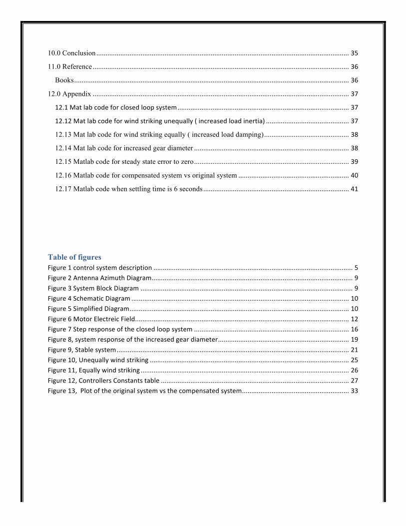
3.0 System Parameters

Parameter Configuration V -­‐ N -­‐ K 2 K1 100 a 50 Ra 10 Ja 0.03 Da 0.02 Kb 1 Kt 1 N1 40 N2 200 N3 250 JL 4 DL 2 Parameter Configuration K pot in 2 K pot out 1.5 K1 100 a 50 Km 0.5263 am 1.053

Kg1 0.2 Kg2 0.8 Table 1, System parameters

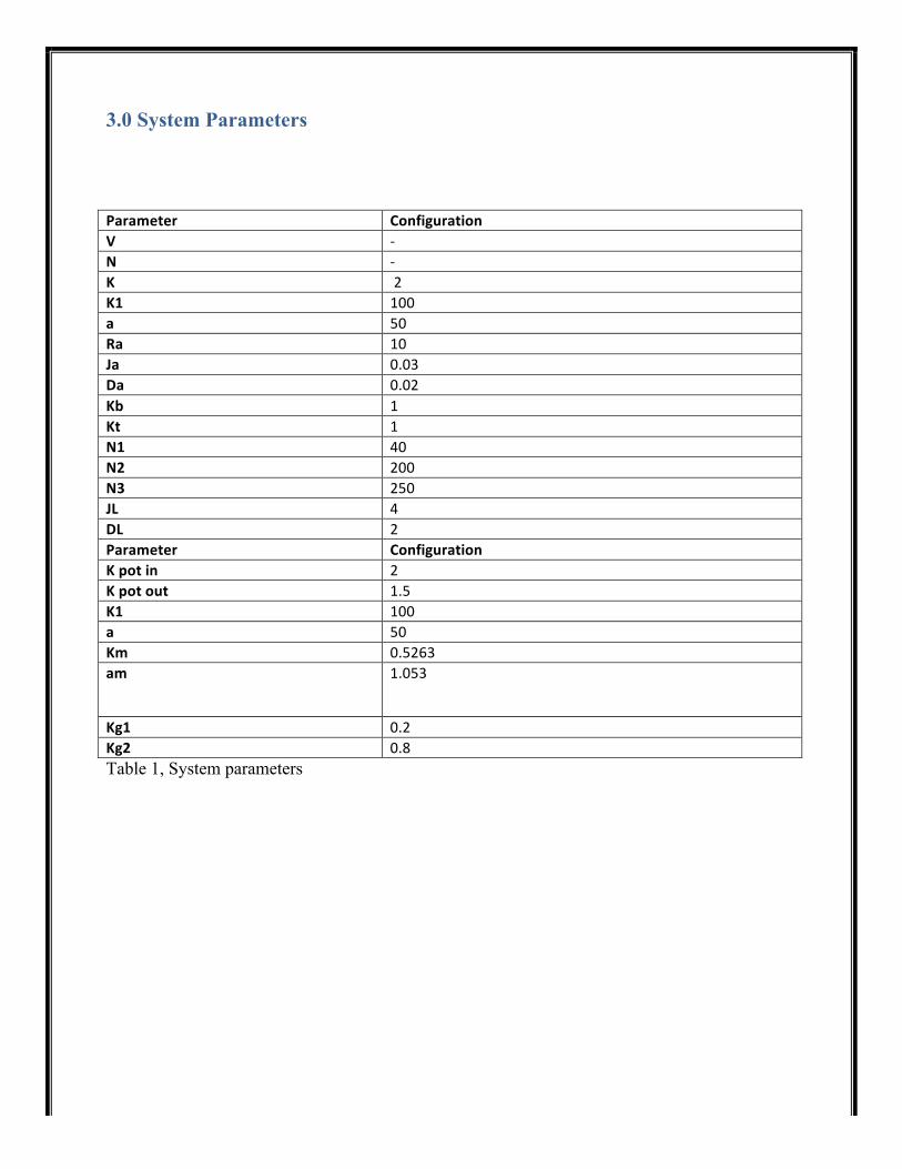
4.0 System Diagram

Figure 2 Antenna Azimuth Diagram

Figure 2, System Diagram (Norman S. Nise, 2011).

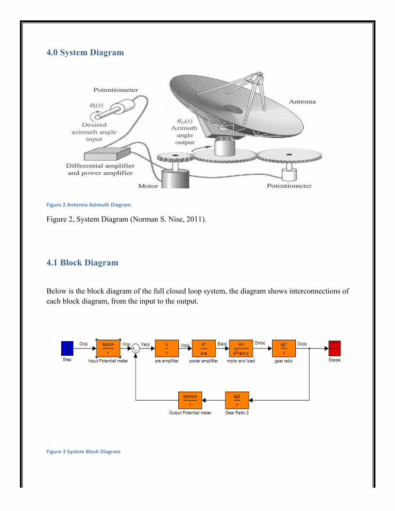
4.1 Block Diagram

Below is the block diagram of the full closed loop system, the diagram shows interconnections of each block diagram, from the input to the output.

Figure 3 System Block Diagram

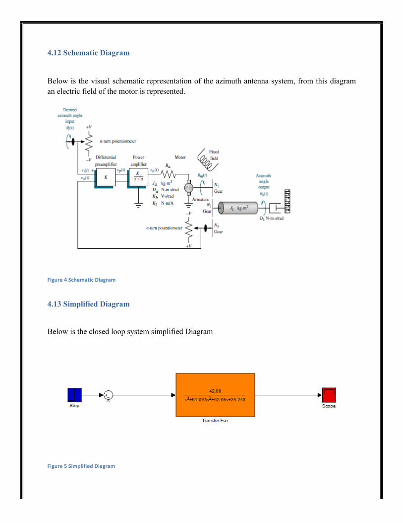
4.12 Schematic Diagram

Below is the visual schematic representation of the azimuth antenna system, from this diagram an electric field of the motor is represented.

Figure 4 Schematic Diagram

4.13 Simplified Diagram

Below is the closed loop system simplified Diagram

Figure 5 Simplified Diagram

5.0 Modeling

5.1 Subsystem 1

The first subsystem is given as the ratio of voltage produced after conversion of angular displacement made by the potential meter, and the value is recorded as potential meter input gain.

!" !!" !

= 𝑘𝑝𝑜𝑡𝑖𝑛 = 2 …………………………………………………………………………...................... (1)

5.12 Subsystem 2

The second subsystem is taken as a ratio of input voltage and output voltage which further can be used by the power amplifier, the result is given as differential amplifier gain

!" !! !"

= 𝐾………………………………………………………………………(2)

5.13 Subsystem 3

The third subsystem is given as a ratio of the voltage which is going to be used by the motor with the output voltage produced from the pre amplifier, this voltage produced will be used to drive the motor

!" !!" !

= !!!!!

= !""!!!"

………………………………………………………………..(3)

5.14 Subsystem 4

It is from this stage where the value of motor and load gain and motor and load pole is going to

be determined. In this stage there is an electric field surrounding the motor, and from this field

the values of inertia and damping are going to be obtained in relation to load and rotor.

Figure 6 Motor Electreic Field

From the circuit above one can see that there is an armature current flowing through the system,

so by Kirchhoff’s voltage low, the following equations are derived.

𝑅𝑎𝑖𝑎 𝑡 + 𝐿𝑎 !"!"

+ 𝑉𝑏 𝑡 − 𝐸𝑎 𝑡 = 0………………………………………………… (4)

One can see that the equation above is in time domain, so by applying Laplace transform the

system is converted to frequency domain.

𝑅𝑎𝐼𝑎(𝑠)+ 𝐿𝑎𝑆𝐼𝑎 + 𝑉𝑏 𝑠 = 𝐸𝑎 𝑠 ………………………………………………………… (5)

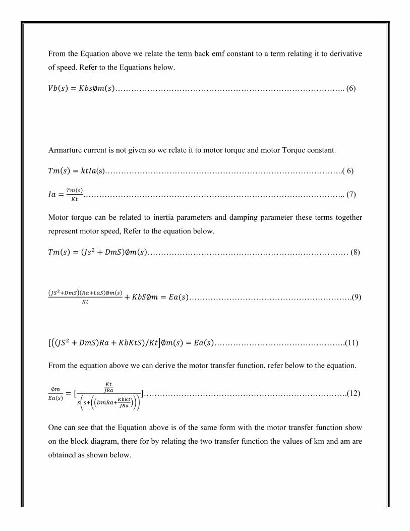
From the Equation above we relate the term back emf constant to a term relating it to derivative

of speed. Refer to the Equations below.

𝑉𝑏 𝑠 = 𝐾𝑏𝑠∅𝑚 𝑠 ………………………………………………………………………….. (6)

Armarture current is not given so we relate it to motor torque and motor Torque constant.

𝑇𝑚 𝑠 = 𝑘𝑡𝐼𝑎(s)……………………………………………………………………………..( 6)

𝐼𝑎 = !" !!"

…………………………………………………………………………………….. (7)

Motor torque can be related to inertia parameters and damping parameter these terms together

represent motor speed, Refer to the equation below.

𝑇𝑚 𝑠 = 𝐽𝑠! + 𝐷𝑚𝑆 ∅𝑚 𝑠 ………………………………………………………………… (8)

!!!!!"# !"!!"# ∅! !!!

+ 𝐾𝑏𝑆∅𝑚 = 𝐸𝑎(𝑠)…………………………………………………….(9)

[ 𝐽𝑆! + 𝐷𝑚𝑆 𝑅𝑎 + 𝐾𝑏𝐾𝑡𝑆)/𝐾𝑡 ∅𝑚(𝑠) = 𝐸𝑎 𝑠 ………………………………………….(11)

From the equation above we can derive the motor transfer function, refer below to the equation.

∅!!" !

= [!"!"#

! !! !"#$!!"!#!"#

]………………………………………………………………….(12)

One can see that the Equation above is of the same form with the motor transfer function show

on the block diagram, there for by relating the two transfer function the values of km and am are

obtained as shown below.

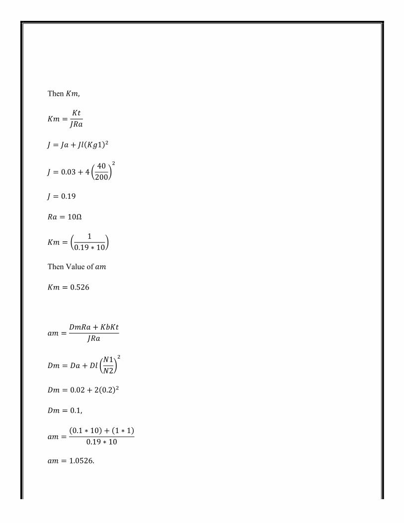
Then 𝐾𝑚,

𝐾𝑚 =𝐾𝑡𝐽𝑅𝑎

𝐽 = 𝐽𝑎 + 𝐽𝑙 𝐾𝑔1 !

𝐽 = 0.03+ 440200

!

𝐽 = 0.19

𝑅𝑎 = 10Ω

𝐾𝑚 =1

0.19 ∗ 10

Then Value of 𝑎𝑚

𝐾𝑚 = 0.526

𝑎𝑚 =𝐷𝑚𝑅𝑎 + 𝐾𝑏𝐾𝑡

𝐽𝑅𝑎

𝐷𝑚 = 𝐷𝑎 + 𝐷𝑙𝑁1𝑁2

!

𝐷𝑚 = 0.02+ 2 0.2 !

𝐷𝑚 = 0.1,

𝑎𝑚 =0.1 ∗ 10 + 1 ∗ 1

0.19 ∗ 10

𝑎𝑚 = 1.0526.

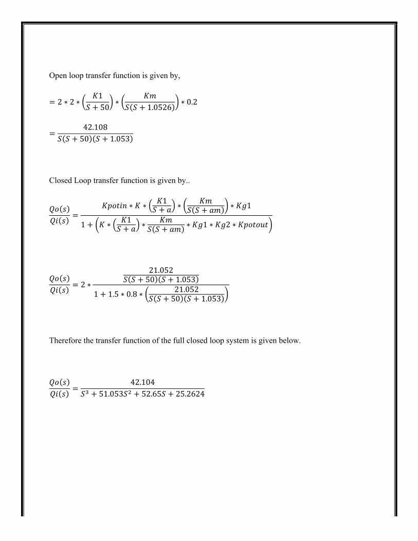
Open loop transfer function is given by,

= 2 ∗ 2 ∗𝐾1

𝑆 + 50 ∗𝐾𝑚

𝑆 𝑆 + 1.0526 ∗ 0.2

=42.108

𝑆 𝑆 + 50 𝑆 + 1.053

Closed Loop transfer function is given by..

𝑄𝑜 𝑠𝑄𝑖 𝑠 =

𝐾𝑝𝑜𝑡𝑖𝑛 ∗ 𝐾 ∗ 𝐾1𝑆 + 𝑎 ∗ 𝐾𝑚

𝑆 𝑆 + 𝑎𝑚 ∗ 𝐾𝑔1

1+ 𝐾 ∗ 𝐾1𝑆 + 𝑎 ∗ 𝐾𝑚

𝑆 𝑆 + 𝑎𝑚 ∗ 𝐾𝑔1 ∗ 𝐾𝑔2 ∗ 𝐾𝑝𝑜𝑡𝑜𝑢𝑡

𝑄𝑜 𝑠𝑄𝑖 𝑠 = 2 ∗

21.052𝑆 𝑆 + 50 𝑆 + 1.053

1+ 1.5 ∗ 0.8 ∗ 21.052𝑆 𝑆 + 50 𝑆 + 1.053

Therefore the transfer function of the full closed loop system is given below.

𝑄𝑜 𝑠𝑄𝑖 𝑠 =

42.104𝑆! + 51.053𝑆! + 52.65𝑆 + 25.2624

6.0 Plot Of The System Response

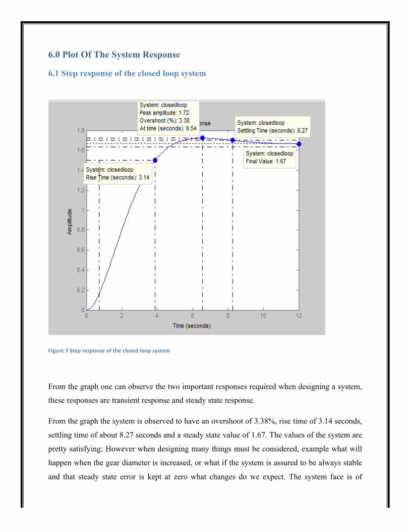
6.1 Step response of the closed loop system

Figure 7 Step response of the closed loop system

From the graph one can observe the two important responses required when designing a system,

these responses are transient response and steady state response.

From the graph the system is observed to have an overshoot of 3.38%, rise time of 3.14 seconds,

settling time of about 8.27 seconds and a steady state value of 1.67. The values of the system are

pretty satisfying; However when designing many things must be considered, example what will

happen when the gear diameter is increased, or what if the system is assured to be always stable

and that steady state error is kept at zero what changes do we expect. The system face is of

concave surface so it is likely to be affected by wind, so one can consider what will the system

respond if the wind strikes equally or un equally across the face of the antenna. All these

conditions are discussed below with the aid of calculations and diagrams.

7.0 Discussion

7.1 Response of the system when the gear attached to the antenna is increased

Gear diameter is proportional to gear teeth; therefore increased gear diameter means increased

number of teeth. Inertia and damping parameters are dependent of gear ratio. Gear attached to

the antenna is gear 2. Thus means if the diameter of the gear 2 increases inertia and damping

parameters will decrease leading to a slower system due to reduced motor speed which is

dependent to inertia and damping. Therefore an increase in gear diameter attached to the antenna

is expected to produce a slower system response. This information is proved below by

calculation and graphs of system response.

𝐾!! =𝑁!𝑁!

=40400

= 0.1

𝐽 = 𝐽! + 𝐽! 𝐾!! !

∴ 𝐽 = 0.03 + 4(0.1)! = 0.07

𝐾! =𝐾!𝐽𝑅!

∴ 𝐾! =1

0.07×10= 1.429

𝐷 = 𝐷! + 𝐷! 𝐾!! !

∴ 𝐷 = 0.02 + 2(0.1)! = 0.04

𝑎! =𝐷!𝑅! + 𝐾!𝐾!

𝐽𝑅!

∴ 𝑎! =0.04×10 + (1×1)

0.07×10= 2

𝜃!(𝑠)𝜃!(𝑠)

=𝐾!"#$% 𝐾× 𝐾!

𝑠 + 𝑎 × 𝐾!𝑠 𝑠 + 𝑎!

×𝐾!!

1 + 𝐾× 𝐾!𝑠 + 𝑎 × 𝐾!

𝑠 𝑠 + 𝑎!×𝐾!!×𝐾!!

∴𝜃!(𝑠)𝜃!(𝑠)

=2×2× 100

(𝑠 + 50)×1.429𝑠(𝑠 + 2)×0.1

1 + 2× 100(𝑠 + 50)×

1.429𝑠(𝑠 + 2)×0.1×1.6×1.5

∴𝜃!(𝑠)𝜃!(𝑠)

=57.16

𝑠! + 52𝑠! + 100𝑠 + 68.592

As our expectation form the above discussion, one can observe that both inertia and damping

parameter to be reduced compared the original system, this technically means the motor speed

will reduce since it is dependent to these parameters, this will lead to a slower system and a

reduced overshoot. Below is the plot of the system response under this condition.

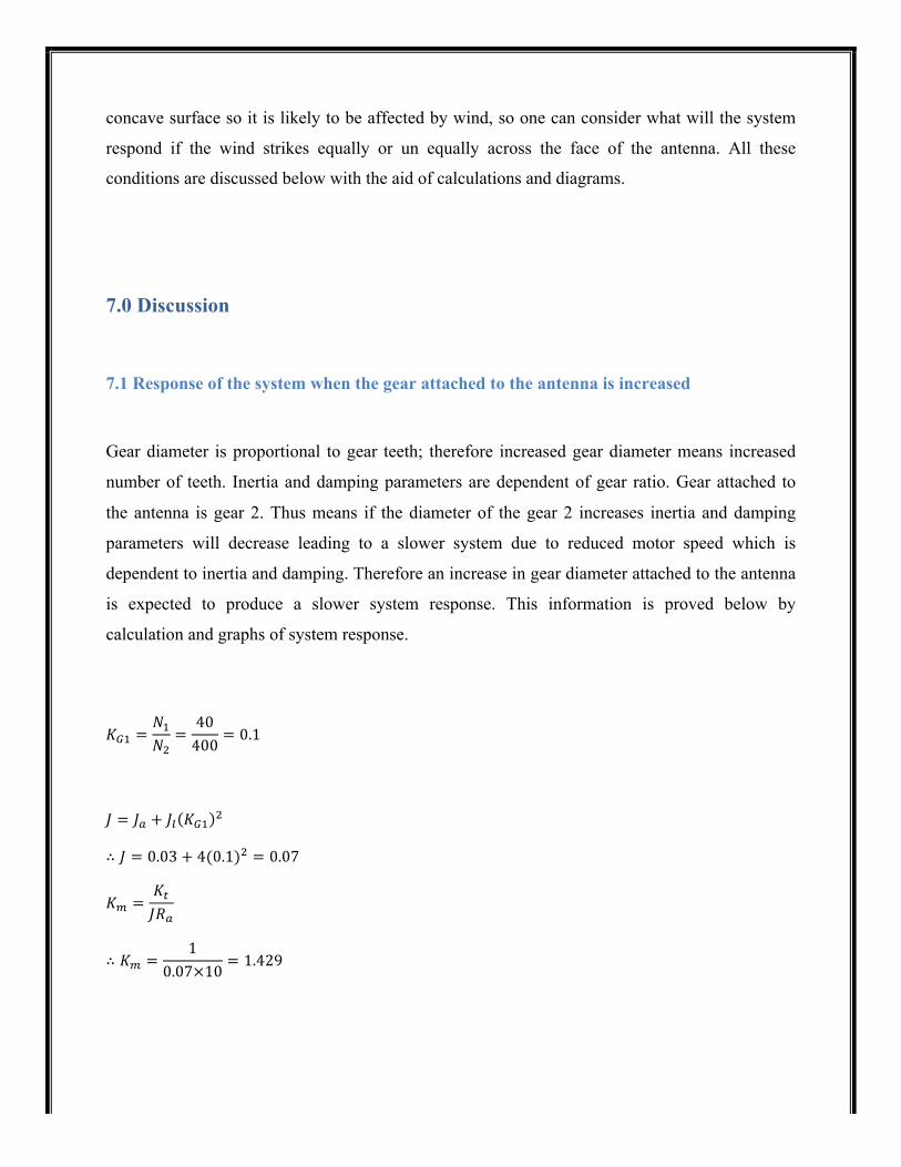
7.12 Plot of the System Response after an Increased Gear Diameter

Figure 8, system response of the increased gear diameter

In general, fast response is accompanied by larger overshoot and consequently shorter time for

the process to “SETTLE OUT.” Conversely, if the response is slower, the process tends to slide

into the final value with little or no overshoot. The requirements of the system dictate which

action is desired.

From the graph we observe that the system has a low overshoot meaning that the system takes

time to reach the desired value, proving the expectations we expected for an increased gear

diameter. In this test the gear teeth is assumed to increase by a hundred percent from 200 to 400

teeth.

7.13 If the System is assured to be always stable and that steady state error is zero

For a steady state error to be zero some of the systems parameters are needed to be changed, our

system does not give a unit feedback that’s why the steady state error is not zero. By reduce the

potentiometer to a gain of one and by making the feedback system to unity, one can observe the

system to have a steady state error at zero and a reduced overshoot. Below is the mathematical

derivation of a unit potentiometer gain with a unit feedback system.

𝜃!(𝑠)𝜃!(𝑠)

=𝐾!!"#$ 𝐾× 𝐾!

𝑠 + 𝑎 × 𝐾!𝑠 𝑠 + 𝑎!

×𝐾!!

1 + 𝐾× 𝐾!𝑠 + 𝑎 × 𝐾!

𝑠 𝑠 + 𝑎!×𝐾!!×𝐾!!

Kpotin= 1 (assumed)

Kg2*kpotout=1 unit feedback (assumed)

𝜃!(𝑠)𝜃!(𝑠)

=

21.052𝑆 𝑆+ 50 𝑆+ 1.053

1+ 1 ∗ 21.052𝑆 𝑆+ 50 𝑆+ 1.053

𝑄𝑜 𝑠𝑄𝑖 𝑠 =

21.052𝑆! + 51.053𝑆! + 52.65𝑆 + 21.052

7.14 Plot of the stable system with steady state error zero

Figure 9, Stable system

From the above graph one can see that the system is fall at a steady state value meaning that the

error have been reduced to zero for a step system with a unit feedback as shown above.

Furthermore the graphs show the settling time is almost the same to the original system and that

the overshoot of the original system have been reduced to half. This response is obtained after

the input potentiometer gain is reduced to one and the feedback system is reduced to a unit

feedback.

7.15 Wind striking across the surface of the plate

In this case they are two possibilities which can happen. The first possibility is that, if the wind

is striking unequally across the surface of the plate, and the second is, if the wind is striking

equally across the surface of the plate.

They are assumption made for all these two scenarios and relevant results are expected. For the

first case, it is assumed that the wind is coming from the east and strikes at the west face of the

concave surface while the east face there is negligible wind force, when this happens the it is

expected the system response to be first because the antenna direction is clockwise and that the

wind is adding more force to it to continue moving a same direction making the load inertia to

increase. Motor speed is a term related to inertia and damping hence if one of the parameters

increase, the motor speed also increases, therefore the system is assumed to give a fast output

response.

The second scenario is when the wind force is striking equally at the surface of the concave face,

in this case the load at the top of the antenna is increasing due to wind force, and this will result

to an increase of load damping, as a scientific proof when damping across the two objects

increases, speed is decreased. Therefore the damping in this scenario is assumed to increase

hence the system speed is expected to give a slow system response. Below are mathematical

derivations for each case.

When load inertia increases to a hundred percent,

𝐾!! =𝑁!𝑁!

=40200

= 0.2

𝐾!! =𝑁!𝑁!

=200250

= 0.8

𝐽 = 𝐽! + 𝐽! 𝐾!! = 0.03 + 8(0.2)! = 0.35

𝐾! =𝐾!𝐽𝑅!

=1

(0.35)(10)= 0.2857

𝐷! = 𝐷! + 𝐷!𝐾!!! = 0.02 + 2 0.2! = 0.1

𝑎! =𝐷!𝑅! + 𝐾!𝐾!

𝐽𝑅!=

0.1 10 + (1)(1)(0.35)(10)

= 0.5714

𝜃!(𝑆)𝜃!(𝑠)

=𝐾!"# !"×𝐾×

𝐾!𝑠 + 𝑎×

𝐾!𝑠(𝑠 + 𝑎!)

×𝐾!!

1 + 𝐾× 𝐾!𝑠 + 𝑎×

𝐾!𝑠(𝑠 + 𝑎!)

×𝐾!!×𝐾!!×𝐾!"# !"

𝜃!(𝑆)𝜃!(𝑠)

=2×2× 100

𝑠 + 50×0.2857

𝑠(𝑠 + 0.5714)×0.2

1 + 2× 100𝑠 + 50×

0.2857𝑠(𝑠 + 0.5714)×0.2×0.8×1.5

𝜃!(𝑆)𝜃!(𝑠)

=

22.856(𝑠 + 50)(𝑠)(𝑠 + 0.5714)

1 + 13.7136(𝑠 + 50)(𝑠)(𝑠 + 0.5714)

𝜃!(𝑆)𝜃!(𝑠)

=

22.856(𝑠 + 50)(𝑠)(𝑠 + 0.5714)

𝑠 + 50 𝑠 𝑠 + 0.5714 + 13.7136(𝑠 + 50)(𝑠)(𝑠 + 0.5714)

𝜃!(𝑆)𝜃!(𝑠)

=22.856

𝑠 + 50 𝑠 𝑠 + 0.5714 + 13.7136

𝜃!(𝑆)𝜃!(𝑠)

=22.856

𝑠! + 50 𝑠 + 0.5714 + 13.7136

𝜃!(𝑆)𝜃!(𝑠)

=22.856

𝑠! + 0.5714𝑠! + 50𝑠! + 28.57𝑠 + 13.7136

𝜃!(𝑆)𝜃!(𝑠)

=22.856

𝑠! + 50.5714𝑠! + 28.57𝑠 + 13.7136

Above is the transfer function of the system when load inertia is increased.

When load damping is increased by a hundred percent,

𝐾!! =𝑁!𝑁!

=40200

= 0.2

𝐾!! =𝑁!𝑁!

=200250

= 0.8

𝐽 = 𝐽! + 𝐽! 𝐾!! = 0.03 + 4(0.2)! = 0.19

𝐾! =𝐾!𝐽𝑅!

=1

(0.19)(10)= 0.5263

𝐷! = 𝐷! + 𝐷!𝐾!!! = 0.02 + 4 0.2! = 0.18

𝑎! =𝐷!𝑅! + 𝐾!𝐾!

𝐽𝑅!=

0.18 10 + (1)(1)(0.19)(10)

= 1.4737

𝜃!(𝑆)𝜃!(𝑠)

=𝐾!"# !"×𝐾×

𝐾!𝑠 + 𝑎×

𝐾!𝑠(𝑠 + 𝑎!)

×𝐾!!

1 + 𝐾× 𝐾!𝑠 + 𝑎×

𝐾!𝑠(𝑠 + 𝑎!)

×𝐾!!×𝐾!!×𝐾!"# !"

𝜃!(𝑆)𝜃!(𝑠)

=2×2× 100

𝑠 + 50×0.5263

𝑠(𝑠 + 1.4737)×0.2

1 + 2× 100𝑠 + 50×

0.5263𝑠(𝑠 + 1.4737)×0.2×0.8×1.5

𝜃!(𝑆)𝜃!(𝑠)

=42.11

𝑠! + 51.47𝑠! + 73.68𝑠 + 25.26

Above is the system transfer function when load damping is increased.

7.16 Plot of the system when wind strikes unequally across the surface of the plate

Figure 10, Unequally wind striking

From the above the overshoot of the system is very high compared to the original system, this

shows that the system provides a faster response as expected from above discussion. Note that

the inertia is assumed to increase by a hundred percent from 4 to 8.

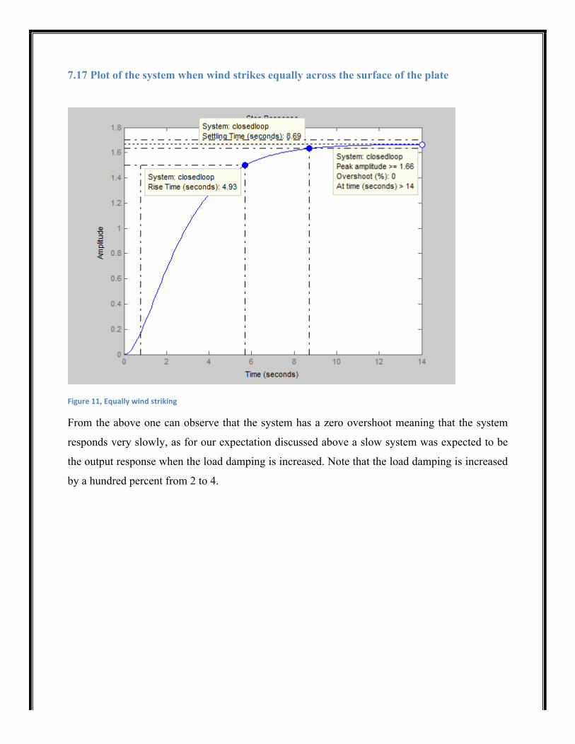
7.17 Plot of the system when wind strikes equally across the surface of the plate

Figure 11, Equally wind striking

From the above one can observe that the system has a zero overshoot meaning that the system

responds very slowly, as for our expectation discussed above a slow system was expected to be

the output response when the load damping is increased. Note that the load damping is increased

by a hundred percent from 2 to 4.

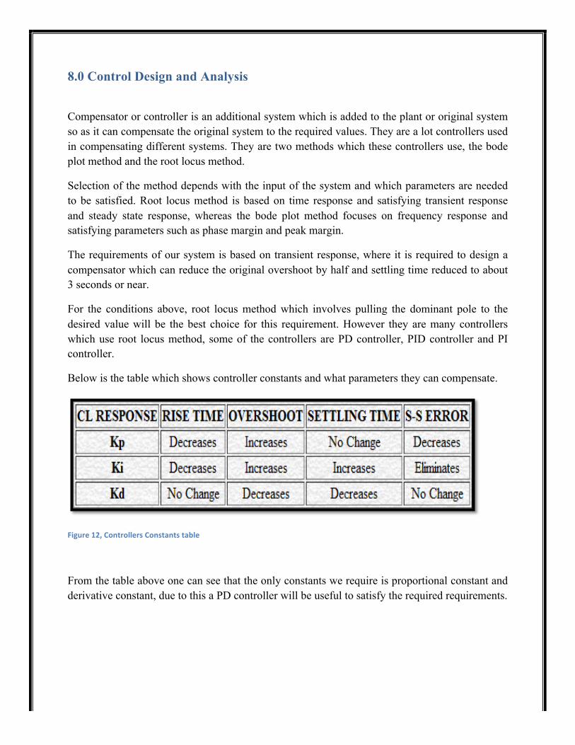
8.0 Control Design and Analysis

Compensator or controller is an additional system which is added to the plant or original system so as it can compensate the original system to the required values. They are a lot controllers used in compensating different systems. They are two methods which these controllers use, the bode plot method and the root locus method.

Selection of the method depends with the input of the system and which parameters are needed to be satisfied. Root locus method is based on time response and satisfying transient response and steady state response, whereas the bode plot method focuses on frequency response and satisfying parameters such as phase margin and peak margin.

The requirements of our system is based on transient response, where it is required to design a compensator which can reduce the original overshoot by half and settling time reduced to about 3 seconds or near.

For the conditions above, root locus method which involves pulling the dominant pole to the desired value will be the best choice for this requirement. However they are many controllers which use root locus method, some of the controllers are PD controller, PID controller and PI controller.

Below is the table which shows controller constants and what parameters they can compensate.

Figure 12, Controllers Constants table

From the table above one can see that the only constants we require is proportional constant and derivative constant, due to this a PD controller will be useful to satisfy the required requirements.

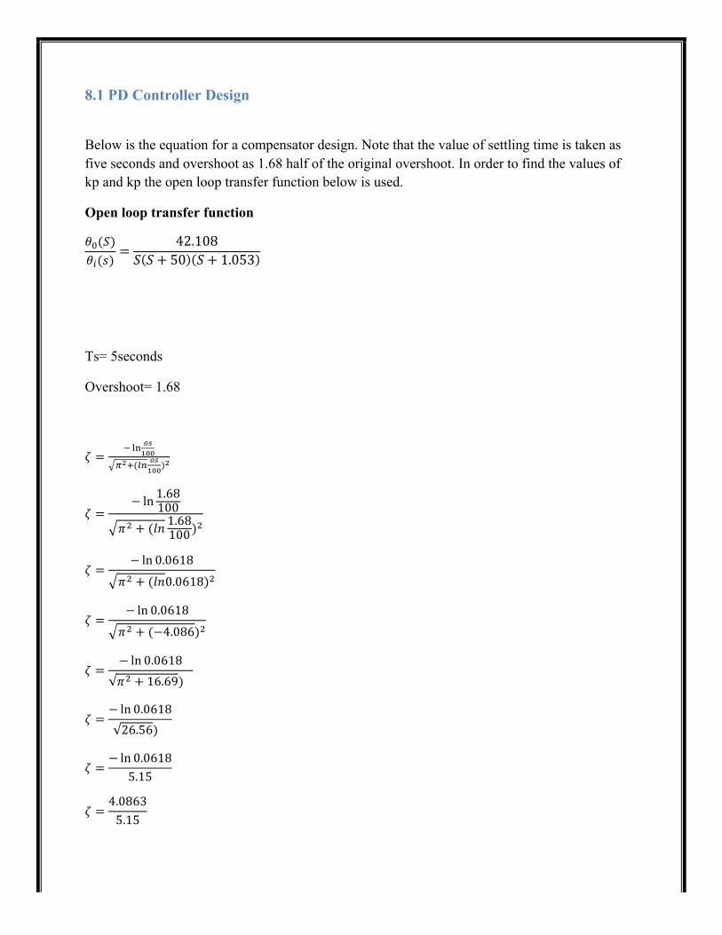
8.1 PD Controller Design

Below is the equation for a compensator design. Note that the value of settling time is taken as five seconds and overshoot as 1.68 half of the original overshoot. In order to find the values of kp and kp the open loop transfer function below is used.

Open loop transfer function

𝜃!(𝑆)𝜃!(𝑠)

=42.108

𝑆 𝑆+ 50 𝑆+ 1.053

Ts= 5seconds

Overshoot= 1.68

𝜁 =! !" !"

!""!!!(!" !"

!"")!

𝜁 =− ln 1.68100

𝜋! + (𝑙𝑛 1.68100)!

𝜁 =− ln 0.0618

𝜋! + (𝑙𝑛0.0618)!

𝜁 =− ln 0.0618

𝜋! + (−4.086)!

𝜁 =− ln 0.0618𝜋! + 16.69)

𝜁 =− ln 0.061826.56)

𝜁 =− ln 0.0618

5.15

𝜁 =4.08635.15

𝜁 = 0.79

TS= !!"#

𝜔𝑛 =4𝑇𝑠𝜁

𝜔𝑛 = !!∗!.!"

=1.01

𝑠𝑑 = −𝜁𝜔𝑛 + 𝜔𝑛 1 − 𝜁!

𝑠𝑑 = −(0.79 ∗ 1.01) + 1.01 1 − 0.79!

𝑠𝑑 = −(0.79 ∗ 1.01) + 1.01 1 − 0.6241

𝑠𝑑 = −(0.79 ∗ 1.01) + 1.01 0.3759

𝑠𝑑 = − 0.79 ∗ 1.01 + 1.01 ∗ 0.613

𝑠𝑑 = − 0.79 ∗ 1.01 + 0.619

𝑠𝑑 = −0.797 + 𝑗0.619

𝐷 = (−.797)! + (0.619)!

𝐷 = (0.64 + 0.3831)

𝐷 = 1.65

𝐷 = 1.0114

𝛽 = 180 − 𝑡𝑎𝑛!!(0.6190.79

)

𝛽 = 180 − 𝑡𝑎𝑛!!(0.78)

𝛽 = 180 − 38.08

𝛽 = 142

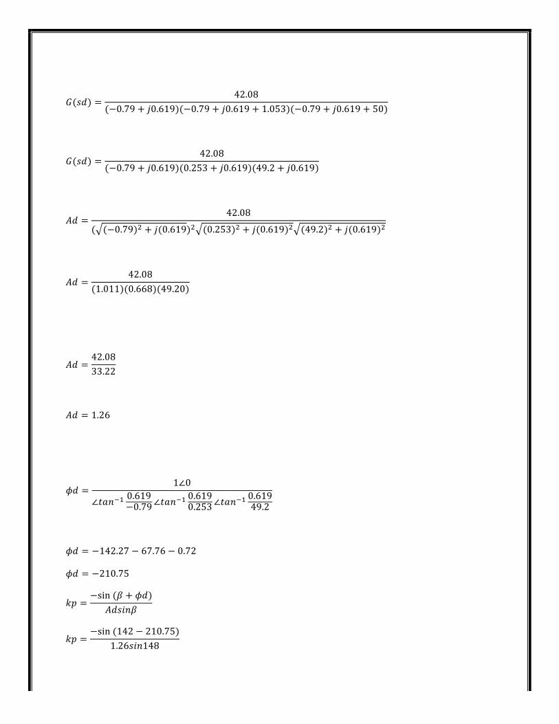
𝐺(𝑠𝑑) =42.08

(−0.79 + 𝑗0.619)(−0.79 + 𝑗0.619 + 1.053)(−0.79 + 𝑗0.619 + 50)

𝐺(𝑠𝑑) =42.08

(−0.79 + 𝑗0.619)(0.253 + 𝑗0.619)(49.2 + 𝑗0.619)

𝐴𝑑 =42.08

( (−0.79)! + 𝑗(0.619)! (0.253)! + 𝑗(0.619)! (49.2)! + 𝑗(0.619)!

𝐴𝑑 =42.08

(1.011)(0.668)(49.20)

𝐴𝑑 =42.0833.22

𝐴𝑑 = 1.26

𝜙𝑑 =1∠0

∠𝑡𝑎𝑛!! 0.619−0.79∠𝑡𝑎𝑛!! 0.6190.253∠𝑡𝑎𝑛

!! 0.61949.2

𝜙𝑑 = −142.27 − 67.76 − 0.72

𝜙𝑑 = −210.75

𝑘𝑝 =−sin (𝛽 + 𝜙𝑑)

𝐴𝑑𝑠𝑖𝑛𝛽

𝑘𝑝 =−sin (142 − 210.75)

1.26𝑠𝑖𝑛148

𝑘𝑝 =−sin (−68.75)1.26𝑠𝑖𝑛148

𝑘𝑝 =0.9320.775

𝑘𝑝 = 1.201

𝑘𝑑 =sin𝜙𝑑

𝐴𝑑𝐷𝑠𝑖𝑛𝛽

𝑘𝑑 =sin (−210.75)

1.26 ∗ 1.011𝑠𝑖𝑛142

𝑘𝑑 =sin (−210.75)1.27𝑠𝑖𝑛142

𝑘𝑑 =0.5110.78

𝑘𝑑 = 0.655

After getting the values of kp and kd above the controller transfer function is multiplied with the original transfer function so as to get the compensated transfer function of the system.

𝐺𝑐 𝑠 = 𝑘𝑝 + 𝑘𝑑𝑠 = 𝑘𝑑(𝑘𝑝𝑘𝑑 + 𝑠)

𝐺𝑐 𝑠 = 1.201 + 0.655𝑆

Closed loop transfer function with unity feedback

𝐺 𝑠 =42.108

𝑠! + 51.0523𝑠! + 52.65𝑠1+ 42.108

𝑠! + 51.0523𝑠! + 52.65𝑠 ∗ 1.2

𝑐𝑜𝑚𝑝𝑒𝑛𝑠𝑎𝑡𝑒𝑑 = 𝐺𝑐 𝑠 ∗ 𝐺 𝑠

𝑐𝑜𝑚𝑝𝑒𝑛𝑠𝑎𝑡𝑒𝑑 =42.108

𝑠! + 51.0523𝑠! + 52.65𝑠1+ 42.108

𝑠! + 51.0523𝑠! + 52.65𝑠 ∗ 1.2∗ 1.201 + 0.655𝑆

𝑐𝑜𝑚𝑝𝑒𝑛𝑠𝑎𝑡𝑒𝑑 =27.5124𝑠 + 50.53808

𝑠! + 51.05𝑠! + 79.802𝑠 + 50.53808

The result above is the transfer function of the compensated system

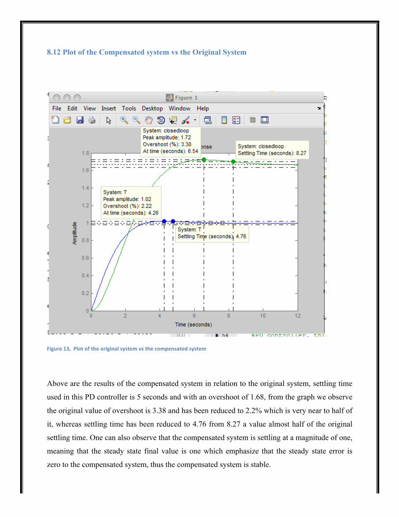
8.12 Plot of the Compensated system vs the Original System

Figure 13, Plot of the original system vs the compensated system

Above are the results of the compensated system in relation to the original system, settling time

used in this PD controller is 5 seconds and with an overshoot of 1.68, from the graph we observe

the original value of overshoot is 3.38 and has been reduced to 2.2% which is very near to half of

it, whereas settling time has been reduced to 4.76 from 8.27 a value almost half of the original

settling time. One can also observe that the compensated system is settling at a magnitude of one,

meaning that the steady state final value is one which emphasize that the steady state error is

zero to the compensated system, thus the compensated system is stable.

The settling time used in this design is 5 seconds, by using the settling time of 3 seconds the

overshoot becomes higher because the system response is very fast, therefore it is decided to use

a settling time higher than 3 seconds so as to compensate the overshoot to a lower value and to

reduce the settling time around 5 seconds. However when settling time is increased more the

system overshoot decreases more, below is the system response when the settling time is

increase to 6 seconds.

Figure 14, system response under 6 seconds settling time

Above is the compensated system response when settling time is 6 seconds, one can observe that

the overshoot has slightly reduced.

9.0 Discussion

By referring above, all mathematical explanation and discussion one each result and response above,

everything is stated above.

The beginning of the project the closed loop differential equations and calculations are obtained and the

system response is plotted and discussed above.

The three cases above are also well analyzed using mathematical equations and graphical representation

and all the results are well discussed.

The last part was the controller, and this was the entertaining part and challenging part of this project, as

observed the PD controller is designed by using an overshoot of 1.68 and settling time of five seconds,

this is because increasing settling time the overshoot is more smoothed than reducing settling time, at first

the settling time of 3 seconds was used and the system responded with an overshoot of 5.14%, so sine the

overshoot was very high it was discussed to increase the settling time to 5seconds and 6 seconds as shown

above from the graphs and the overshoot was observed to reduce by a higher percent up to 2.2% and

1.83% respectively.

10.0 Conclusion

As per requirements of this assignment, all requirements needed are well full filled with potential

outputs, the plot of the closed loop response is satisfied, the three cases are well analyzed and

satisfied with potential outputs and each result is well discussed.

The controller is well designed and it is acceptable design since the product of the absolute of

compensator and our system gives the value one as the answer. The overshoot requirement is

well satisfied together with the settling time.

To sum up a lot of knowledge is learnt in this assignment and how the systems behave in

different conditions, example what happens when overshoot increases, it obvious the system will

respond faster.

11.0 Reference

Books Norman S. Nise, “ Control System Engineering”.

12.0 Appendix

12.1 Mat lab code for closed loop system %%%%%%%%%%%%% Program Designed By ARNOLD GABRIEL%%%%%%%%%%% %closed loop system N1=40; N2=200 N3=250; Ja=0.03 JL=4 Da=0.02 DL=2 Kt=1; Ra=10; Kb=1; kg1=(N1/N2); kg2=(N2/N3); J=Ja+JL*(kg1)^2 Dm=Da+DL*(kg1)^2 a=50; k=2; k1=100; kpotout=1.5; kpotin=2; km=Kt/(J*Ra) am=(Dm*Ra+Kb*Kt)/(J*Ra) G=(kpotin*k*k1*km*kg1); C=tf([G],conv([1 0],conv([1 am],[1 a]))); F=tf([kpotout*kg2/kpotin],[1]); closedloop=feedback(C,F,-1) step(closedloop)

12.12 Mat lab code for wind striking unequally ( increased load inertia) %%%%%%%%%%%%% Program Designed By ARNOLD GABRIEL%%%%%%%%%%% %closed loop system N1=40; N2=200 N3=250; Ja=0.03 JL=8 Da=0.02 DL=2 Kt=1; Ra=10; Kb=1; kg1=(N1/N2); kg2=(N2/N3); J=Ja+JL*(kg1)^2 Dm=Da+DL*(kg1)^2 a=50;

k=2; k1=100; kpotout=1.5; kpotin=2; km=Kt/(J*Ra) am=(Dm*Ra+Kb*Kt)/(J*Ra) G=(kpotin*k*k1*km*kg1); C=tf([G],conv([1 0],conv([1 am],[1 a]))); F=tf([kpotout*kg2/kpotin],[1]); closedloop=feedback(C,F,-1) step(closedloop)

12.13 Mat lab code for wind striking equally ( increased load damping) %%%%%%%%%%%%% Program Designed By ARNOLD GABRIEL%%%%%%%%%%% %closed loop system N1=40; N2=200 N3=250; Ja=0.03 JL=4 Da=0.02 DL=4 Kt=1; Ra=10; Kb=1; kg1=(N1/N2); kg2=(N2/N3); J=Ja+JL*(kg1)^2 Dm=Da+DL*(kg1)^2 a=50; k=2; k1=100; kpotout=1.5; kpotin=2; km=Kt/(J*Ra) am=(Dm*Ra+Kb*Kt)/(J*Ra) G=(kpotin*k*k1*km*kg1); C=tf([G],conv([1 0],conv([1 am],[1 a]))); F=tf([kpotout*kg2/kpotin],[1]); closedloop=feedback(C,F,-1) step(closedloop)

12.14 Mat lab code for increased gear diameter %%%%%%%%%%%%% Program Designed By ARNOLD GABRIEL%%%%%%%%%%% %closed loop system N1=40; N2=400 N3=250; Ja=0.03 JL=4

Da=0.02 DL=2 Kt=1; Ra=10; Kb=1; kg1=(N1/N2); kg2=(N2/N3); J=Ja+JL*(kg1)^2 Dm=Da+DL*(kg1)^2 a=50; k=2; k1=100; kpotout=1.5; kpotin=2; km=Kt/(J*Ra) am=(Dm*Ra+Kb*Kt)/(J*Ra) G=(kpotin*k*k1*km*kg1); C=tf([G],conv([1 0],conv([1 am],[1 a]))); F=tf([kpotout*kg2/kpotin],[1]); closedloop=feedback(C,F,-1) step(closedloop)

12.15 Matlab code for steady state error to zero %%%%%%%%%%%%% Program Designed By ARNOLD GABRIEL%%%%%%%%%%% %closed loop system N1=40; N2=200 N3=200; Ja=0.03 JL=4 Da=0.02 DL=2 Kt=1; Ra=10; Kb=1; kg1=(N1/N2); kg2=(N2/N3); J=Ja+JL*(kg1)^2 Dm=Da+DL*(kg1)^2 a=50; k=2; k1=100; kpotout=1; kpotin=1; km=Kt/(J*Ra) am=(Dm*Ra+Kb*Kt)/(J*Ra) G=(kpotin*k*k1*km*kg1); C=tf([G],conv([1 0],conv([1 am],[1 a]))); F=tf([kpotout*kg2/kpotin],[1]); closedloop=feedback(C,F,-1) step(closedloop)

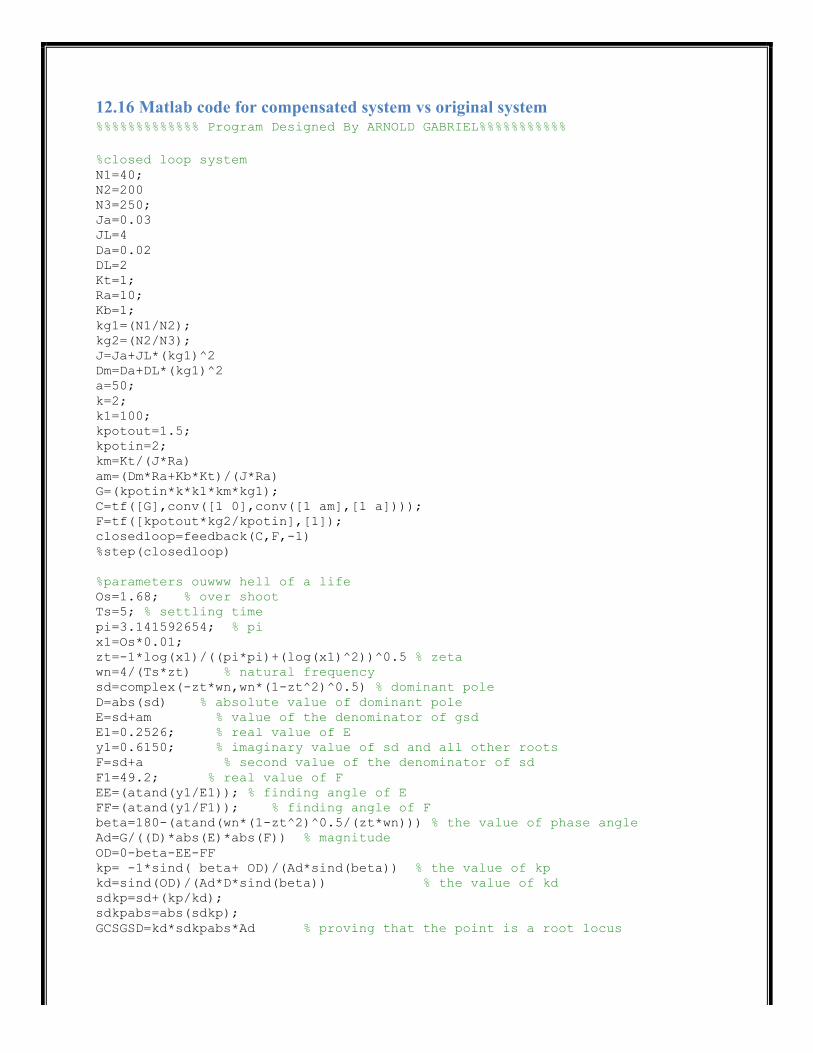
12.16 Matlab code for compensated system vs original system %%%%%%%%%%%%% Program Designed By ARNOLD GABRIEL%%%%%%%%%%% %closed loop system N1=40; N2=200 N3=250; Ja=0.03 JL=4 Da=0.02 DL=2 Kt=1; Ra=10; Kb=1; kg1=(N1/N2); kg2=(N2/N3); J=Ja+JL*(kg1)^2 Dm=Da+DL*(kg1)^2 a=50; k=2; k1=100; kpotout=1.5; kpotin=2; km=Kt/(J*Ra) am=(Dm*Ra+Kb*Kt)/(J*Ra) G=(kpotin*k*k1*km*kg1); C=tf([G],conv([1 0],conv([1 am],[1 a]))); F=tf([kpotout*kg2/kpotin],[1]); closedloop=feedback(C,F,-1) %step(closedloop) %parameters ouwww hell of a life Os=1.68; % over shoot Ts=5; % settling time pi=3.141592654; % pi x1=Os*0.01; zt=-1*log(x1)/((pi*pi)+(log(x1)^2))^0.5 % zeta wn=4/(Ts*zt) % natural frequency sd=complex(-zt*wn,wn*(1-zt^2)^0.5) % dominant pole D=abs(sd) % absolute value of dominant pole E=sd+am % value of the denominator of gsd E1=0.2526; % real value of E y1=0.6150; % imaginary value of sd and all other roots F=sd+a % second value of the denominator of sd F1=49.2; % real value of F EE=(atand(y1/E1)); % finding angle of E FF=(atand(y1/F1)); % finding angle of F beta=180-(atand(wn*(1-zt^2)^0.5/(zt*wn))) % the value of phase angle Ad=G/((D)*abs(E)*abs(F)) % magnitude OD=0-beta-EE-FF kp= -1*sind( beta+ OD)/(Ad*sind(beta)) % the value of kp kd=sind(OD)/(Ad*D*sind(beta)) % the value of kd sdkp=sd+(kp/kd); sdkpabs=abs(sdkp); GCSGSD=kd*sdkpabs*Ad % proving that the point is a root locus

%PD controller, this is entertaining it had me sweat... figure(1) CC=tf(G*[kd kp],conv([1 0],conv([1 1.053],[1 50]))); Fd=tf([1],[1]); T=feedback(CC,Fd,-1) step (T,closedloop);

12.17 Matlab code when settling time is 6 seconds

%%%%%%%%%%%%% Program Designed By ARNOLD GABRIEL%%%%%%%%%%% %closed loop system N1=40; N2=200 N3=250; Ja=0.03 JL=4 Da=0.02 DL=2 Kt=1; Ra=10; Kb=1; kg1=(N1/N2); kg2=(N2/N3); J=Ja+JL*(kg1)^2 Dm=Da+DL*(kg1)^2 a=50; k=2; k1=100; kpotout=1.5; kpotin=2; km=Kt/(J*Ra) am=(Dm*Ra+Kb*Kt)/(J*Ra) G=(kpotin*k*k1*km*kg1); C=tf([G],conv([1 0],conv([1 am],[1 a]))); F=tf([kpotout*kg2/kpotin],[1]); closedloop=feedback(C,F,-1) step(closedloop) %parameters ouwww hell of a life Os=1.68; % over shoot Ts=6; % settling time pi=3.141592654; % pi x1=Os*0.01; zt=-1*log(x1)/((pi*pi)+(log(x1)^2))^0.5 % zeta wn=4/(Ts*zt) % natural frequency sd=complex(-zt*wn,wn*(1-zt^2)^0.5) % dominant pole D=abs(sd) % absolute value of dominant pole E=sd+am % value of the denominator of gsd E1=0.3860; % real value of E y1=0.5125; % imaginary value of sd and all other roots F=sd+a % second value of the denominator of sd F1=49.3333; % real value of F EE=(atand(y1/E1)); % finding angle of E

FF=(atand(y1/F1)); % finding angle of F beta=180-(atand(wn*(1-zt^2)^0.5/(zt*wn))) % the value of phase angle Ad=G/((D)*abs(E)*abs(F)) % magnitude OD=0-beta-EE-FF kp= -1*sind( beta+ OD)/(Ad*sind(beta)) % the value of kp kd=sind(OD)/(Ad*D*sind(beta)) % the value of kd sdkp=sd+(kp/kd); sdkpabs=abs(sdkp); GCSGSD=kd*sdkpabs*Ad % proving that the point is a root locus %PD controller, this is entertaining it had me sweat... figure(1) CC=tf(G*[kd kp],conv([1 0],conv([1 1.053],[1 50]))); Fd=tf([1],[1]); T=feedback(CC,Fd,-1) step (T,closedloop);