azwad tamir et al/ (ijcsit) international journal of

Crime Prediction and Forecasting using Machine

Learning Algorithms Azwad Tamir#1, Eric Watson#, Brandon Willett#, Qutaiba Hasan#, Jiann-Shiun Yuan#2

#Department of ECE, University of Central Florida

4000 Central Florida Blvd, Orlando, FL 32816, USA

[email protected]

[email protected]

Abstract— This research will focus on machine learning

algorithms for crime forecasting. In the modern world, crime is

becoming a major and complex problem. In this research, we

discover the best course of action for teaching a model to forecast

crime in major metropolitan cities. The purpose of this study is

to provide the Police Department with proper crime forecasting

so they can better delegate their resources in response to future

crime hotspots. We applied several machine learning models to

predict the severity of a reported crime based on whether the

crime would lead to an arrest or not. We also did a deep dive into

the city districts and studied the crime trends by year. We used

Folium to do data visualization for the study of these trends. We

discovered trends in the number of crimes and the arrest rate

from year to year. The different machine learning models that

we developed are the Random Forest, K-Nearest-Neighbours,

AdaBoost, and Neural Network. We tested our models on the

Chicago Police Department's CLEAR (Citizen Law Enforcement

Analysis and Reporting) system, which has more than 6,000,000

records. Among all four models, the Neural Network has the best

outcome with an accuracy of 90.77%. This study also provides an

insight into the applicability of different machine learning

models in analyzing crime report datasets from large

metropolitan cities.

Keywords— AdaBoost, crime forecasting, deep neural network,

folium, future crime, KNN, machine learning, prediction,

random forest.

I. INTRODUCTION

Aggressive urbanization is causing a rapid increase in the

size and population of large cities across the world. This

massive population growth in cities is causing total crimes to

rise sharply, making it difficult for the police department to

keep up with it. It is not possible for the police department to

station police officers in every street corner, so they need

some intelligent system that can predict the likelihood of

crimes occurring in different parts of the city at different times

of the day. Also, there is a large volume of emergency 911

calls and crime reports coming at every moment of the day.

These reports need to be sorted to identify the more imminent

threats, so the police department could allocate their resources

accordingly and respond to more alarming situations before

addressing the rest.

These difficulties stimulated a lot of research work in

recent times related to predicting future crimes to help the

police department allocate their resources. S. Kim et al.

proposed different machine learning methods to predict

crimes in Vancouver from crime data in the last 15 years and

obtained an accuracy of 39% and 44% for the K-nearest-

neighbour and boosted decision tree algorithms, respectively

[1]. Y. Lin et al. investigated a deep machine learning model

based on the broken windows and spatial analysis to predict

future crime hotspot locations in Taiwan [2]. P. Kumari et al.

applied Extra Tree Classifier, K-Neighbours, Support Vector

Machines, Decision Tree Classifier, and Neural Network

algorithms to predict the probability of different types of

crimes in different locations and time around the city [3]. N.

Hooda et al. used data obtained from different government

websites to predict future crime rates at different city areas

using the Folium API [4]. W. Gorr et al. analysed crime data

to influence and adjust policies and rules to better adapt for

the future [5]. E. Ahishakiye et al. came up with a machine

learning model using decision trees to categorize crimes based

on the crimes’ text description [7]. H. Nguyen et al. build an

automatic machine learning based classifier that predicts the

severity of a traffic accident based on the incident records [8].

J. Cohen et al. proposed a model for crime forecasting to help

with the allocation of police resources [9]. Lastly, A. Wheeler

et al. used Random Forest to build a long-term crime predictor

of different locations in the city of Dallas.

The objective of our work is to predict the severity of the

crime based on the incident reports. We choose whether an

arrest was made as the indicator representing the crime

severity. We used a dataset of crime reports for the city of

Chicago from the year 2001 to 2018, which was made

available through the Kaggle website [13]. The data came

from the Chicago Police Department's CLEAR (Citizen Law

Enforcement Analysis and Reporting) system and consisted of

more than 6 million records or data points. Each of the data

point has 23 features that represented various information

about the nature, location, time, description, and severity of

the reported crime. We generated four different machine

learning models, namely Random forest, K-nearest-

neighbours (KNN), Adaptive Boost (AdaBoost), and artificial

neural network (NN) to predict whether an arrest was made

based on the information available in the other features of the

dataset. Moreover, we generated detailed analyses relating to

the crimes’ location and trends and visualized them in

interactive maps using the Folium API.

The paper is organized into four subsequent sections.

Section II contains all the data pre-processing and feature

engineering steps taken to clean up the data and prepare it for

Azwad Tamir et al/ (IJCSIT) International Journal of Computer Science and Information Technologies, Vol. 12 (2) , 2021, 26-33

26

implementation. Section III consists of the details of the

model architecture and properties and parameters used to

construct the classifiers. Section IV incorporates the details of

the analysis done on the data and the techniques used to

visualize the trends and crime patterns. Section V reports the

results of the various models and demonstrates the

visualizations. Finally, Section VI concludes the work and

points out potential future research directions.

II. DATA PRE-PROCESSING & FEATURE SELECTION

A series of pre-processing steps were implemented on the

dataset to clean it up and make it ready before inserting them

into the machine learning classifiers. The detailed analysis of

the preprocessing steps taken for each of the features is

provided below:

ID/Case Number: Both the ID and Case Number features

are unique identifiers used to tag each incident or datapoint. It

had unique values for each of the data points and hence did

not contain any information. These features, however, were

used to remove duplicate data from the dataset. After this,

they were not considered and entirely dropped from the

dataset.

Block: This represents the block address of the reported

crimes. There were two parts to this feature. The first was a

set of numbers that denotes the house number of the report

location. The second part consisted of the name of the street of

the reported location. There were several types of

inconsistencies in this feature that were first removed. Some

of these inconsistencies include typos, different terminologies

used for missing datasets, and formatting errors. There were a

few missing values for which the entire row was discarded.

There were too few of them to cause any significant decrease

in the number of datapoints. The next modification was to

separate the number and street name into two different

features. This was done in order to make it easier for the

training models to learn the dataset. Finally, the street names

were encoded into integers for the convenience of storing the

values and loading them into the machine learning models.

Description: This contains the description of a crime in a

concise manner. There were 353 unique description values in

the dataset. As a result, it consists of categorical information

about the nature of the reported crime. The description texts

were encoded into integers to help with the storage and

loading process. The feature data were also checked for

missing values, typos, inconsistencies, and outliers, but none

were found.

IUCR and FBI code: IUCR stands for Illinois Uniform

Crime Reporting, and this was used as a code denoting the

type of crimes reported. The FBI code also contains similar

information about the nature of the crime. These two features

contain information that is very similar to the description

feature, and there also exists a very high correlation among

them. Hence, these features were dropped as this information

is already being feed to the machine learning models through

the description column.

Arrest: This is a binary categorical data that has either true

or false values. True means that an arrest was made for the

reported crime while false refers that no one was arrested for

that crime. This represents the severity of the crime and could

be used to deduce whether imminent police involvement is

required or not. The police department could use this

information to control the allocation of resources and assign

police officers accordingly. So, this was used as the prediction

labels of the machine learning models. The data was also

encoded into binary values for ease of handling.

Domestic: This also consists of binary values and denotes

whether the crime occurred in a domestic or public

environment. Domestic crimes are usually more non-violent

and include domestic disturbance and other related issues. The

data was first encoded into integers and checked for

inconsistencies and missing values. Fortunately, there was no

problem with the data and required no further processing.

District, Ward, and Community Area: These are three

different measures used to divide up the total area under a city.

They contained the location information of the crime report.

However, all of them had a large amount of missing data

points and there exits other location features like the

coordinates and Block which contained very little missing

values and the same information. Hence, all these features

were excluded from the training process.

Beat: This represents the smallest police geographical

segmentation area, which they use to allocate resources. This

feature was already in the form of integers and contained no

missing values, inconsistencies, and outliers. As a result, no

further processing was required.

Latitude and Longitude: These contained the exact

location of the crime’s reporting location in the form of

continuous variables. About 1 percent of the data was missing.

The entire row containing the missing values were excluded

from the dataset. The data also contained some inconsistencies

and outliers. These were dropped as well.

X and Y coordinate: Contains the same information as the

latitude and longitude values in a different format. Hence,

they contained no additional information and were therefore

dropped.

Updated on: This represents when the report was included

in the police server. They show a high correlation to the data

and time features of the dataset and hence were dropped.

Location: Composite of the latitude and longitude columns,

they contained the same information as the latitude and

longitude features and were therefore not included.

Location Description: This is a categorical data that

describes the location of where the crime was committed.

There are over 170 unique values, which were encoded into

integers to make storing the values easier and loading them

into the machine learning model. Over 1,968 null values were

found for this feature, which were dropped from the dataset.

Primary Type: This is a categorical data that describes the

type of crime that was committed. There were over 35 unique

values of this data, which were encoded into integers for

making it more convenient to store values and load them into

the machine learning model. Some unique values also had

lower value counts than others, so values with a count less


27

than 1,000 were removed from the dataset, leaving only 25

unique values for this data.

Date: This data contains the time at which the crime

incident was reported. This feature was used as an index when

pre-processing the dataset and was dropped after it was not

needed.

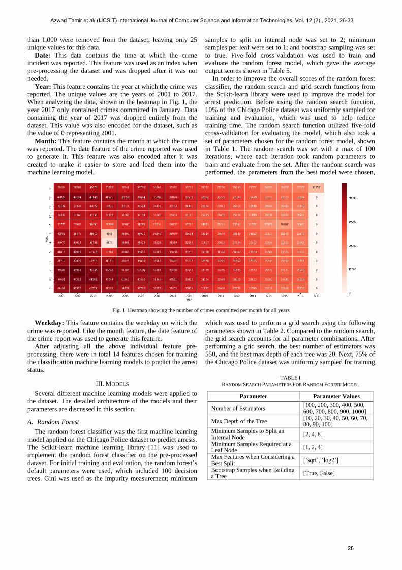
Year: This feature contains the year at which the crime was

reported. The unique values are the years of 2001 to 2017.

When analyzing the data, shown in the heatmap in Fig. 1, the

year 2017 only contained crimes committed in January. Data

containing the year of 2017 was dropped entirely from the

dataset. This value was also encoded for the dataset, such as

the value of 0 representing 2001.

Month: This feature contains the month at which the crime

was reported. The date feature of the crime reported was used

to generate it. This feature was also encoded after it was

created to make it easier to store and load them into the

machine learning model.

Weekday: This feature contains the weekday on which the

crime was reported. Like the month feature, the date feature of

the crime report was used to generate this feature.

After adjusting all the above individual feature pre-

processing, there were in total 14 features chosen for training

the classification machine learning models to predict the arrest

status.

III. MODELS

Several different machine learning models were applied to

the dataset. The detailed architecture of the models and their

parameters are discussed in this section.

A. Random Forest

The random forest classifier was the first machine learning

model applied on the Chicago Police dataset to predict arrests.

The Scikit-learn machine learning library [11] was used to

implement the random forest classifier on the pre-processed

dataset. For initial training and evaluation, the random forest’s

default parameters were used, which included 100 decision

trees. Gini was used as the impurity measurement; minimum

samples to split an internal node was set to 2; minimum

samples per leaf were set to 1; and bootstrap sampling was set

to true. Five-fold cross-validation was used to train and

evaluate the random forest model, which gave the average

output scores shown in Table 5.

In order to improve the overall scores of the random forest

classifier, the random search and grid search functions from

the Scikit-learn library were used to improve the model for

arrest prediction. Before using the random search function,

10% of the Chicago Police dataset was uniformly sampled for

training and evaluation, which was used to help reduce

training time. The random search function utilized five-fold

cross-validation for evaluating the model, which also took a

set of parameters chosen for the random forest model, shown

in Table 1. The random search was set with a max of 100

iterations, where each iteration took random parameters to

train and evaluate from the set. After the random search was

performed, the parameters from the best model were chosen,

which was used to perform a grid search using the following

parameters shown in Table 2. Compared to the random search,

the grid search accounts for all parameter combinations. After

performing a grid search, the best number of estimators was

550, and the best max depth of each tree was 20. Next, 75% of

the Chicago Police dataset was uniformly sampled for training,

Fig. 1 Heatmap showing the number of crimes committed per month for all years

TABLE I

RANDOM SEARCH PARAMETERS FOR RANDOM FOREST MODEL

Parameter Parameter Values

Number of Estimators [100, 200, 300, 400, 500, 600, 700, 800, 900, 1000]

Max Depth of the Tree [10, 20, 30, 40, 50, 60, 70, 80, 90, 100]

Minimum Samples to Split an Internal Node

[2, 4, 8]

Minimum Samples Required at a Leaf Node

[1, 2, 4]

Max Features when Considering a Best Split

[‘sqrt’, ‘log2’]

Bootstrap Samples when Building a Tree

[True, False]


28

while the remaining 25% were used for the test set. Compared

to the scores using the default parameters, the accuracy

increased around 3.98%, precision improved around 11.88%,

recall increased around 2.46%, and the f1 score increased

around 6.66%. The performance results of the tuned random

forest model are shown in Table 5.

B. K-Nearest Neighbours

The k-nearest neighbors classifier was the second machine

learning model used on the Chicago Police dataset to predict

arrests. Like the random forest classifier, the Scikit-learn

library was used to implement the k-NN classifier on the

dataset. For initial training and evaluation, the default

parameters of the k-NN classifier were used, with a K value

equal to 5 and the distance measurement being set as

Euclidean. The Five-fold cross-validation was used to train

and evaluate the k-NN model, which gave the average output

scores shown in Table 5.

In order to improve the k-NN model, the random search

function from Scikit-learn was used to find the best

parameters for the model, where the parameters chosen are

shown in Table 3. Like the random forest model, 10% of the

dataset was uniformly sampled for training/evaluating the

model, where 100 iterations were used for the random search

along with the five-fold cross-validation. The best model gave

the following parameters: k = 11, weights = ‘distance’,

algorithm = ‘ball_tree’, leaf_size = 20, and p = 1. A grid

search was not further needed for this model, so the

parameters from the best model in the random search were

used for training and evaluating the model. Like the random

forest model, 75% of the dataset was uniformly sampled, and

the remaining was used for the test set. The performance of

the tuned k-NN model is shown in Table 5. The k-NN

accuracy increased around 0.94%, precision increased around

4.07%, recall decreased around 0.49%, and f1 score increased

around 0.41%. Overall, compared to the random forest model,

the k-NN model did not show significant improvement apart

from a slight increase in precision.

C. AdaBoost

The adaptive boost classifier was the third machine

learning model used on the Chicago Police dataset to predict

arrests. Like the previous two models, the Scikit-learn library

was used to implement the adaptive boost classifier on the

dataset. For training and evaluating the classifier, five-fold

cross-validation was used and the default parameters of the

AdaBoost model were used. The default parameters include a

learning rate of 1; 200 weak classifiers; and a max depth of 1

for each decision tree classifier. The model’s performance

with the default parameters is shown in Table 5, which was

shown to be lower in performance than the random forest

model, which is more likely due to it being more susceptible

to noise in the data.

Like the previous two classifiers, the Scikit-learn functions

were used to help tune the model. Given that the only

important parameters to tune were the number of estimators

and the learning rate, a grid search technique was used as

there were fewer parameter combinations to work with

compared to the other models. The parameters chosen for the

estimators were: 400, 500, and 600. Also, learning rates of 1,

1.2, 1.4, 1.6, 1.8, and 2 were considered. Like the previous

models, 10% of the dataset was uniformly sampled for

training and evaluating the model, where five-fold cross-

validation was used for the grid search. The parameters from

the best model were a number of estimators equal to 600, and

a learning rate equal to 1.8. After the best parameters were

found, 75% of the dataset was uniformly sampled for training

and the remaining 25% was used for the test set to evaluate

the model. The performance of the tuned AdaBoost model is

shown in Table 5. The accuracy of the model increased

around 2.05%, precision decreased around 0.82%, recall

increased around 8.55%, and the f1 score increased around

TABLE III

GRID SEARCH PARAMETERS FOR RANDOM FOREST MODELS


Number of Estimators [450, 500, 550]

Max Depth of the Tree [15, 20, 25]

Minimum Samples to Split an Internal Node

[2]

Minimum Samples Required at a Leaf Node

[2]

Max Features when Considering a Best Split

[‘log2’]

Bootstrap Samples when Building a Tree

[False]

TABLE III

RANDOM SEARCH PARAMETERS FOR KNN MODEL


Number of Neighbors [3, 5, 7, 9, 11, 13]

Weights (Function used in Prediction) [‘uniform’, ‘distance’]

Algorithm (Used for nearest neighbors computation)

[‘ball_tree’, ‘kd_tree’]

Leaf Size (Used for BallTree or KDTree) [20, 30, 40]

Power Parameter (Used for Minkowski Metric)

[1, 2]

TABLE IV

MODEL PROPERTIES AND HYPERPARAMETERS OF NN MODEL

Parameter Description Value

Loss Function Cross Entropy Loss

Optimizer Adam Optimizer

Test Train Split Fivefold cross validation

Output Class 2

Batch Size 1000

Learning Rate 0.01

Number of Training Epochs 500


29

6.31%. Overall, this led to the AdaBoost classifier performing

best after the random forest classifier, which has the k-NN

classifier perform below the AdaBoost classifier.

D. Neural Network

The last classification machine learning model that we trained

on the Chicago Police dataset to predict arrest was a neural

network based classifier. Four different models that varied in

architecture and number of layers were trained on the dataset,

and their test accuracies were compared. The first model

consisted of 4 hidden layers, the second model had 6 hidden

layers, whereas the third model contained 11, and the fourth

had 14 hidden layers. The PyTorch machine learning

programming framework [12] was used to generate all the

models. The Neural network consisting of 11 hidden layers

showed the best performance. The basic architecture of this

network is shown in Fig. 2.

The input layer consists of 14 features. Then the

information propagates through 11 hidden layers of varying

width. The RELU activation function was used in between

each hidden layer. Other activation functions were also tried

out, but The RELU showed the best accuracy. The layers

became wider while going further down towards the middle

and then was shrank down to 14 nodes and was finally

converged to 2 neurons as the output was a binary

classification. The architecture followed a type of double

wedge shape with a wide middle with a narrow head and a tail.

A SoftMax layer was used at the end to predict the

classification label.

A couple of additional data preprocessing was done to help

the training of the model and avoid overfitting. The number of

data points after the initial preprocessing contained 6.08

million samples where 72% were negative samples and the

rest 28% were positive. So, the data was moderately skewed

and confused the network, and made it harder to learn. So, a

random sampling was done to reduce the data to 2.90 million,

where a fraction of the negative samples was discarded. This

made the data more uniform and easier to learn with 52% of

the new dataset being negative and the rest 48% being positive.

Finally, a normalization was applied on all the different

features of the dataset by subtracting each value with the mean

and dividing it with the standard deviation.

The properties and hyperparameters of the network are

shown in table 4. A wide range of different hyperparameter

values was tried out with a grid search to pick the most

optimum hyperparameters that produced the best results. The

Cross-Entropy loss function was used along with an Adam

optimizer. 20% of the data was set aside for the testing and the

remaining 80% was used for training the model. A batch size

of 100 was used while training at a learning rate of 0.01 and

the model was trained for 100 epochs. The training accuracy

achieved after 100 epochs was about 92% with a 90.77% test

accuracy so the model was not overfitted.

IV. DATA VISUALIZATION

When analyzing the dataset, the heatmap shown in Fig. 1

was first used to determine whether crimes were decreasing or

increasing. It was found to be gradually going down over the

years. Next, the crimes were analyzed per month to observe

which months have the highest crime rates, which is shown in

Fig. 3. The month of July was determined to be where crimes

peak the highest, while February showed the lowest crime

rates. Crimes per week were further analyzed, and it was

Input Layer: 14 Features

Layer1: Number of Nodes: 28, Activation:RELU











Output Layer: Number of nodes: 2

Fig. 2 The detailed architecture of the best performing neural network

model

Fig. 3 Distribution of crimes in different days of the week

Fig. 4 Distribution of crimes in different month of the year


30

determined that Friday has the highest number of crimes,

while Sunday has the lowest number of crimes.

Crimes per location were also analyzed after performing

temporal analysis on the dataset. Viewing crimes based on

location revealed that the highest number of crimes were

committed on the street, followed by crimes committed at

residencies, crimes committed at apartments, and crimes

committed at sidewalks. Crimes per type were also analyzed,

where theft had the highest crime count, followed by battery,

criminal damage, and narcotics.

After data preprocessing and investigation, we noticed a

trend with the data based on year. We started plotting out the

crime locations, and color coded them based on whether there

was an arrest or not for each year. We noticed an increase in

arrests in 2004-2005 and then a decrease in arrests made in

2006 shown in Fig. 4. Please note in Fig. 4, we are comparing

2005 and 2006 as this shows the largest change in crime rates

in two consecutive years. In Fig. 5, we visualized the Arrest

rates per district and the number of incidences per district.

This would help point out the districts that need more

workforce as there is an obvious lack of resources in these

districts needed to keep up with the crime. Please note in Fig.

5, we are comparing the entire data on a district level. We

compare the arrest rates with the number of incidents to see if

there is a correlation. What we discovered was that some

districts with a high arrest rate were due to the low number of

incidents, while the districts with the higher number of

incidents have a lower arrest rate. Note that there were two

districts with a high number of incidents which also have a

decent arrest rate. The data visualized in Fig. 5 will help focus

down the areas that need to be patrolled more frequently and

need more assistance or funding. All visualizations in this

section were made using the Folium API.

V. RESULTS

The arrest status was predicted using the preprocessed

dataset generated in Section II with the machine learning

models described in Section III. Initially, the default

parameter values of the Scikit-learn library were used to

generate the accuracy parameters. Later, extensive model

parameter tuning described in Section III was implemented to

increase the models’ performance by significant amounts. The

corresponding values for the performance metrics of the

Random Forest, k-nearest-neighbors, and AdaBoost machine

learning algorithms before and after parameter tuning are

shown in Table 5. The comparison between the pretuned and

tuned accuracies and F1 scores is given in Fig. 6, while that

between precision and recall is given in Fig. 7.

The results showed an increase in all three models’ overall

accuracy after tuning compared to their pre-tuned counterparts

with the most significant increase for the Random forest

classifier. However, the accuracy of k-NN did not improve

much during the tuning process. A large increase in precision

TABLE V

PERFORMANCE OF MODELS WITH DEFAULT AND TUNED PARAMETERS

Models Average Accuracy Average Precision Average Recall Average F1 Score

Pre-tuned models with

default parameters

Random Forest 84.878% 80.276% 63.826% 70.446%

k-NN (k = 5) 84.071% 78.756% 59.974% 68.094%

AdaBoost 85.859% 91.105% 55.791% 68.824%

Model with tuned

parameters

Random Forest 88.861% 92.156% 66.283% 77.107%

k-NN (k = 5) 85.008% 82.825% 59.482% 69.239%

AdaBoost 87.914% 90.281% 64.344% 75.137%

Fig. 5 Comparing 2005 and 2006 locational data based on arrests. Red

dots represent crime reports and blue dot represents an arrest was made

based on the report.

Fig. 6 Comparing the total of arrest rates per district to the total number

of incidents per district. Note that the two places with the lowest number

of incidents also have the highest arrest rate.


31

was seen for the Random Forest classifier after tuning, with a

significant increase for the k-NN algorithm as well. However,

the precision value of the AdaBoost algorithm had in fact

decreased after the tuning process. On the other hand,

AdaBoost had a considerable enhancement in the recall value,

while that of Random Forest and k-NN did not change much

due to the parameter tuning. Finally, a significant increase in

the F1 score was seen for the Random forest and the

AdaBoost algorithm with very little change in that of k-NN

after the tuning process. Overall, the Random forest and the

AdaBoost showed better performance in terms of the Average

accuracy and the F1 score among the three conventional

machine learning models.

Finally, four different Neural Network (NN) models with

varying architecture were trained on the dataset to predict the

police report’s arrest status. The hyperparameters of all four

neural network architectures trained on the dataset were

extensively tuned, and their accuracy parameters were

compared to figure out the best model. The results obtained

for the different neural network models are given in Table 6.

The test accuracy and other performance metrics of the neural

network model before and after hyperparameter tuning are

shown in Table 7. A Significant boost in the performance of

the model was observed after tuning the hyperparameters. The

final test accuracy came up to be 90.77%, which is greater

than all the other models that we trained. The Precision,

Recall, and F1 score of the neural network is also more

impressive compared to the other models.

The comparison between the tuned and final versions of

all four machine learning models, namely the Random forest,

k-NN, AdaBoost, and neural network are given in Fig. 8. It

shows the Neural Network has better performance than the

other models in all the different performance metrics. This is

especially prominent in the Precision, Recall and F1 scores of

the different models.

VI. CONCLUSION

In this work, we applied K-Nearest Neighbors, AdaBoost,

Random Forest, and Neural Network algorithms to form

models to forecast future crimes and locations of crimes. Also,

we visualized the data using the Folium API for our data

breakdown. The neural network based machine learning

TABLE VI

PERFORMANCE OF DIFFERENT NEURAL NETWORK MODELS

Number of Layers

Test Accuracy (%)

Precision Recall F-1

Score 4 89.97 0.955 0.828 0.887 6 90.43 0.959 0.835 0.893

11 90.77 0.962 0.837 0.895 14 90.31 0.958 0.833 0.891

TABLE VII

PERFORMANCE OF NN MODELS AFTER PARAMETER TUNING

Performance Metric

Results obtained before

hyperparameter tuning

Results obtained after

hyperparameter tuning

Accuracy 84.971% 90.771%

Precision 89.416% 96.198%

Recall 72.729% 83.706%

F1 Score 80.214% 89.518%

Fig. 7 Comparison between pretuned and tuned accuracies and F1 Scores

between the different conventional ML models.

Fig. 8 Comparison between pretuned and tuned precision and recall

between the different conventional ML models.

Fig. 9 Comparison between the performance metrics of all four ML

Models


32

model performed the best among the different algorithms

achieving an impressive accuracy of 90.77%. It also showed

better performance in terms of precision, recall and F-1 scores

compared to the other machine learning models. We also

implemented several different neural network models with

varying architectures and number of layers to determine the

best structure for this kind of dataset. This work would help

the police department of large metropolitan cities determine

which police calls need imminent attention and manage their

resources accordingly. It would also help them plan which

areas of the city would require more police involvement in the

future.

REFERENCES

[1] S. Kim, P. Joshi, P. S. Kalsi, and P. Taheri, "Crime Analysis Through

Machine Learning," in 2018 IEEE 9th Annual Information Technology,

Electronics and Mobile Communication Conference (IEMCON), 1-3

Nov. 2018 2018, pp. 415-420, doi: 10.1109/IEMCON.2018.8614828.

[2] Y. Lin, T. Chen, and L. Yu, "Using Machine Learning to Assist Crime

Prevention," in 2017 6th IIAI International Congress on Advanced

Applied Informatics (IIAI-AAI), 9-13 July 2017 2017, pp. 1029-1030,

doi: 10.1109/IIAI-AAI.2017.46.

[3] Pratibha, A. Gahalot, Uprant, S. Dhiman, and L. Chouhan, "Crime

Prediction and Analysis," in 2nd International Conference on Data,

Engineering and Applications (IDEA), 28-29 Feb. 2020 2020, pp. 1-6,

doi: 10.1109/IDEA49133.2020.9170731.

[4] A. Jawla, M. Singh, and N. Hooda, "Crime Forecasting using Folium,"

Test Engineering and Management, vol. 82, pp. 16235-16240, 05/31

2020.

[5] W. Gorr and R. Harries, "Introduction to crime forecasting,"

International Journal of Forecasting, vol. 19, no. 4, pp. 551-555,

2003/10/01/ 2003, doi: https://doi.org/10.1016/S0169-2070(03)00089-

X.

[6] M. Granroth-Wilding and S. Clark, "What Happens Next? Event

Prediction Using a Compositional Neural Network Model," in AAAI,

2016.

[7] E. Ahishakiye, E. Opiyo, and I. Niyonzima, "Crime Prediction Using

Decision Tree (J48) Classification Algorithm," International Journal

of Computer and Information Technology (ISSN: 2279 – 0764), 05/15

2017.

[8] H. Nguyen, C. Cai, and F. Chen, "Automatic classification of traffic

incident's severity using machine learning approaches," IET Intelligent

Transport Systems, vol. 11, 07/14 2017, doi: 10.1049/iet-its.2017.0051.

[9] J. Cohen, W. L. Gorr, and A. M. Olligschlaeger, "Leading Indicators

and Spatial Interactions: A Crime-Forecasting Model for Proactive

Police Deployment," Geographical Analysis,

https://doi.org/10.1111/j.1538-4632.2006.00697.x vol. 39, no. 1, pp.

105-127, 2007/01/01 2007, doi: https://doi.org/10.1111/j.1538-

4632.2006.00697.x.

[10] A. P. Wheeler and W. Steenbeek, "Mapping the Risk Terrain for

Crime Using Machine Learning," Journal of Quantitative Criminology,

2020/04/24 2020, doi: 10.1007/s10940-020-09457-7.

[11] F. Pedregosa et al., "Scikit-learn: Machine learning in Python," the

Journal of machine Learning research, vol. 12, pp. 2825-2830, 2011.

[12] A. Paszke et al., "Pytorch: An imperative style, high-performance deep

learning library," arXiv preprint arXiv:1912.01703, 2019.

[13] An extensive dataset of crimes in Chicago (2001-2017), by City of

Chicago. [Online]. Available:

https://www.kaggle.com/currie32/crimes-in-chicago

[14] Y.-L. Lin, M.-F. Yen, and L.-C. Yu, "Grid-Based Crime Prediction

Using Geographical Features," ISPRS International Journal of Geo-

Information, vol. 7, no. 8, p. 298, 2018. [Online]. Available:

https://www.mdpi.com/2220-9964/7/8/298.

[15] P. Stalidis, T. Semertzidis, and P. Daras, "Examining deep learning

architectures for crime classification and prediction," arXiv preprint

arXiv:1812.00602, 2018.

[16] Z. M. Wawrzyniak et al., "Data-driven models in machine learning for

crime prediction," in 2018 26th International Conference on Systems

Engineering (ICSEng), 18-20 Dec. 2018 2018, pp. 1-8, doi:

10.1109/ICSENG.2018.8638230.

[17] M. S. Islam, M. S. Rahman, and M. A. Amin, "Beat Based Realistic

Dance Video Generation using Deep Learning," in 2019 IEEE

International Conference on Robotics, Automation, Artificial-

intelligence and Internet-of-Things (RAAICON), 29 Nov.-1 Dec. 2019

2019, pp. 43-47, doi: 10.1109/RAAICON48939.2019.22.

[18] S. A. Chun, V. A. Paturu, S. Yuan, R. Pathak, V. Atluri, and N. R.

Adam, "Crime Prediction Model using Deep Neural Networks,"

presented at the Proceedings of the 20th Annual International

Conference on Digital Government Research, Dubai, United Arab

Emirates, 2019. [Online]. Available:

https://doi.org/10.1145/3325112.3328221.

[19] A. M. Shermila, A. B. Bellarmine, and N. Santiago, "Crime Data

Analysis and Prediction of Perpetrator Identity Using Machine

Learning Approach," in 2018 2nd International Conference on Trends

in Electronics and Informatics (ICOEI), 11-12 May 2018 2018, pp.

107-114, doi: 10.1109/ICOEI.2018.8553904.

[20] H. K. R. ToppiReddy, B. Saini, and G. Mahajan, "Crime Prediction &

Monitoring Framework Based on Spatial Analysis," Procedia

Computer Science, vol. 132, pp. 696-705, 2018/01/01/ 2018, doi:

https://doi.org/10.1016/j.procs.2018.05.075.

[21] N. H. M. Shamsuddin, N. A. Ali, and R. Alwee, "An overview on

crime prediction methods," in 2017 6th ICT International Student

Project Conference (ICT-ISPC), 23-24 May 2017 2017, pp. 1-5, doi:

10.1109/ICT-ISPC.2017.8075335.


33

https://doi.org/10.1016/S0169-2070(03)00089-X

https://doi.org/10.1016/S0169-2070(03)00089-X

https://doi.org/10.1111/j.1538-4632.2006.00697.x

https://doi.org/10.1111/j.1538-4632.2006.00697.x

https://doi.org/10.1111/j.1538-4632.2006.00697.x

https://www.kaggle.com/currie32/crimes-in-chicago

https://www.mdpi.com/2220-9964/7/8/298

https://doi.org/10.1145/3325112.3328221

https://doi.org/10.1016/j.procs.2018.05.075

azwad tamir et al/ (ijcsit) international journal of

Documents