1

BUBBLING OVER ALONG THE OIL FUTURES YIELD CURVE

Daniel Tsvetanov, Jerry Coakley, Neil Kellard

Essex Business School, University of Essex

December 2013

Abstract

We employ novel tests to investigate WTI crude oil spot and futures prices

along the yield curve for the presence of rational bubbles. The empirical

methodology adopted is consistent with periods of multiple bubbles and

permits the origination and end dates of each bubble to be identified. The

results indicate that all but the spot and nearby series exhibit significant

bubble periods ending in late 2008. Moreover, the dating algorithms

establish that the bubbles in longer-dated contracts start much earlier and

are longer lasting than the bubble in the 3- to 12-month contracts. This

information from the oil futures yield curve suggests a period of disconnect

between the spot and longer dated futures contracts from 2004 to late 2008

which coincides with a spell of increased institutional investment in oil

futures.

JEL code: G10, C15, C22

Keywords: Multiple bubbles; Spot and futures prices; Bubble dating

algorithm; Bubble duration.

2

1 Introduction

The equilibrium price of a security with infinite maturity equals its fundamental

value plus a bubble component. When the bubble grows and dominates the

fundamental value, it induces explosive behaviour in the price series. Exploiting

this property, we apply a battery of tests to examine the null hypothesis that there

is no bubble in spot and futures oil prices. We include in our analysis contracts

with maturities of up to twenty four months to account for differing investment

strategies along the yield curve. To the best of our knowledge, this is the first

paper to investigate bubbles in crude oil futures prices across the spectrum of

maturities out to two years. We employ the dating strategy introduced by Phillips,

Shi, and Yu (2012 to identify the origination and end dates of the bubbles. This

strategy can take into account the possibility of multiple bubbles and consistently

estimates the origination and collapse dates of each bubble even when they are of

different magnitude.

This paper employs monthly data 1995M09-2012M04 to investigate the time

series properties of WTI crude oil spot and (3- to 24-month) futures contracts

listed on NYMEX. Our empirical analysis produces some novel results. Firstly,

while the spot and nearby contracts exhibit no evidence of bubbles according to

two of our three dating procedures, all other series exhibited extended periods of

bubble behaviour that end in late 2008. This paper is the first to find evidence of

this striking disconnect which is difficult to reconcile with rational behaviour

3

using standard models.1 Secondly, the dating algorithms indicate that the bubble

in longer-dated contracts started much earlier and were longer lasting than the

bubble in the 6-to 12-month contracts. For instance the results from all three data

stamping procedures indicate a continuous bubble for 24-month contract over the

2004-2008 period. Finally, the evidence for contracts 15 through to 24 suggest

that the bubbles originated in early 2004.

Our results are consistent with the findings of Buyuksahin, Haigh, Harris,

Overdahl, and Robe (2009). They utilise a unique CFTC Large Trader Reporting

System (LTRS) position dataset, which allows them to investigate the evolution of

futures trading activity by trader type and contract maturity. They argue that the

positions of hedge funds and non-registered participants in long-dated futures

have increased significantly since early 2004-2005. However, hedge funds are

often recognised as sophisticated institutional investors. Their trading activities

would correct for any price deviations from fundamental levels and contribute

towards market efficiency, preventing the occurrence of bubbles (see Fama,

1965). Contrary to the efficient market prospective, Abreu and Brunnermeier

(2003) consider an economy where rational agents would deliberately allow

bubbles to persist. Hedge funds may have been aware of the mispricing of long-

dated futures but preferred to benefit from it rather than correct it.

Our paper contributes to the financialisation debate. The origination date of

bubble periods found in the longer-dated futures contracts coincides with the

sharp increase of investor interest in commodity markets. Tang and Xiong (2012)

1 Jarrow and Protter (2009) investigate asset price bubbles under arbitrage free pricing theory in

incomplete markets. Using a local martingale framework they show that futures prices can possess

bubbles that are independent from the underlying asset’s price bubble.

4

argue that from 2004 commodity futures markets entered an era of

financialization. Commodities were then viewed as a distinct investment category

and began to co-move positively with equity markets. In addition, Sockin and

Xiong (2013) show how institutional investors might have contributed towards

the commodity boom and bust cycles in 2007-2008. This has caused serious

concerns among practitioners and policy makers that excessive speculation might

have been the main driver of rising energy and food prices (see, e.g., Masters

(2008), Soros (2008), US Senate Permanent Subcommittee on Investigations

(2006)). However, our new results do not necessarily imply that excessive

speculation in commodity futures markets contributed towards price deviations

away from fundamental levels in the physical market. One of the challenges in

evaluating this hypothesis is the lack of relevant data on institutional commodity

contract positions over a sufficiently long period of time. Further empirical

analysis is needed to clarify the potential source of bubble behaviour that we

document.

Our results are closely related to those of Shi and Arora (2012) and Phillips

and Yu (2011) who explore the crude oil market for bubble behaviour. Shi and

Arora (2012) use the convenience yield implied by the nearest and second nearest

contracts in three different regime switching models. They find a short-lived

bubble in late 2008 and early 2009. Phillips and Yu (2011) apply a recursive right

tail unit-root test, originally proposed by Phillips, Wu, and Yu (2009), to the spot

price and again find a short bubble episode between March and July 2008. They

show a potential transmission mechanism. The bubble behaviour in oil markets

appears to have migrated from the housing market. We adopt the same recursive

5

framework but introduce a series of other tests to provide robustness check on

our findings.

Unlike these studies, we do not constrain our analysis by focusing on the

price behaviour of only the spot or nearby futures contracts. Instead, we test for

bubbles in the crude oil market along the spectrum oil futures yield curve from 1

to 24 months. In this sense, our paper also contributes to a strand of literature that

investigates the role of futures markets in the process of price discovery. Futures

contracts are not redundant securities and they are priced in conjunction with the

spot contract. In an economy with risk neutral and rational agents, the

contemporaneous futures price for delivery at a specified date should be an

unbiased predictor of the future spot price. We show that, under the theory of

rational bubbles, the futures price consists of the fundamental value and a bubble

component at the maturity date of the contract. If a bubble develops, it should

affect the time series properties of the futures contract earlier than the spot.

However, while this is consistent with the episodes of bubble behaviour for 2008

in our results, it contradicts the earlier disconnect of longer-dated futures from the

spot market.

The reminder of the paper is organised as follows. In section 2, we provide

some theoretical background on the price-bubble relationship for storable

commodities. We outline the motivations behind the used empirical methodology.

Sections 3 and 4 describe the econometric approach for the purposes of our

analysis. In Section 5, we present the data, provide some descriptive statistics. The

empirical results are discussed in Section 6. Finally, Section 7 concludes.

6

2 The theory of rational bubbles in commodity markets

We follow Diba and Grossman (1988b) and explain the price change of storable

commodities by the changes in expected future net payoffs defined as

"fundamentals'. The current spot price of a commodity, , is determined by the

present value of next period's expected spot price, , and marginal

convenience yield, :

(1)

where denotes the expectation conditional on the information at time . is a

time invariant interest rate. The net of storage cost marginal convenience yield

measures the benefit from holding inventories per unit of commodity over the

period to and is analogous to the dividend on a stock. Under the theory of

storage it should satisfy the standard no arbitrage condition

(2)

where denotes the futures price at time for delivery of a commodity at .

If and are both integrated processes, the series are cointegrated with specific

cointegrating vector (see Campbell and Shiller (1987)). Solving (2) for

and extracting from both sides, it follows that the difference between the

futures and spot prices is the interest forgone in storing the commodity over the

period to , less the marginal convenience yield.

Solving the difference equation (1) forward and applying the low of iterated

expectations, yields

7

[∑

]

[

] (3)

Imposing the transversality condition eliminates the

last term in (3). It follows that the price collapses to the discounted sum of

expected future payoffs, i.e. the fundamental value which will be denoted by

.

However, if the transversality condition does not hold, there are infinitely many

solutions to (3) that take the form:

(4)

where is a bubble component that has to satisfy:

(5)

In other words, the bubble has to grow over time at a rate in order for investors

agree to hold the asset (see Blanchard and Watson (1982)). Diba and Grossman

(1988a) argued that rational bubbles cannot be negative. If a bubble is negative,

then when it erupts, it could make the price of the security negative also. In

addition, if , (5) implies that with probability 1. It follows that the

existence of bubbles would be consistent with rationality only when .

Taken together, equations (1) and (2) imply that the futures price is an

unbiased predictor of the future spot price

(6)

Given the decomposition of the spot price in (5), it follows that the

contemporaneous futures price with maturity embodies information about

the expected value of the bubble component over the period to

8

[

] (7)

In line with (5), the bubble is expected to grow exponentially at rate , i.e.

contains the root that is greater than unity. If the bubble erupts at some

future time , for , it will induce an explosive behaviour in the price

series futures contracts with maturity greater than .

To test for rational bubbles in the stock market, Diba and Grossman (1988b)

motivated the use of stationarity tests. However, Evans (1991) suggested that this

approach would not efficiently detect periods of explosive behaviour if bubbles

collapse periodically. Consistent with the process in (5), he considers bubbles

described by:

{ }

{ } (8)

where , is a positive iid variable with , and { }

is an indicator function that assumes a value of 1 when the condition in the braces

is true and 0 otherwise. is an iid Bernoulli process and the probability of

is and is , where . Such a bubble would start

to grow at a rate once it exceeds some threshold level , but with a

probability the bubble will collapse to an expected mean level . Since a

bubble never collapses to zero it will start growing again without violating the

non-negativity constraint given in Diba and Grossman (1988).

The non-linear bubble process in (8) causes the data series to exhibit

characteristics similar to an integrated or even a stationary process. As a result,

conventional unit root tests applied to the full sample would fail adequately to test

9

the null hypothesis of no bubbles and could lead to false negatives. Phillips, Wu,

and Yu (2011) suggested the application of a unit root test in a recursive window

framework to overcome this drawback. Their approach allows the statistics to be

time dependent and is able to detect explosive behaviour in time series even when

bubbles are periodically collapsing.

3 Testing for explosive behaviour

Suppose we observe the sequence { } and estimate the following

atoregression:

for ⌊ ⌋ and (9)

where is white noise, is a fraction of the total sample and ⌊ ⌋ denotes the

integer part of . The recursive window of the regression expands by one

observation at a time from some initial sample ⌊ ⌋. The tests adopted in our

empirical analysis are performed under the null that the time series contain a unit

root for every :

for ⌊ ⌋ and (10)

Under the alternative hypothesis, Phillips, Wu, and Yu (2011) specified a data

generating process where the series starts as a unit root but switches to a regime

of mildly explosive behaviour ( is greater than unity but still in its vicinity) at

date ⌊ ⌋ until ⌊ ⌋. At date ⌊ ⌋ the series returns to a unit root regime. The

model is defined as:

10

{ ⌊ ⌋} {⌊ ⌋ ⌊ ⌋}

(∑ ⌊ ⌋ ⌊ ⌋

) { ⌊ ⌋} { ⌊ ⌋},

(11)

The restriction on parameter and values of over the specified open interval

yields the mildly explosive process discussed in Phillips and Magdalinos (2007a,

2007b). The boundary as includes the local to unity case where defining a

bubble period is not possible (see Phillips and Yu (2011)).

Phillips, Wu, and Yu (2011) suggested the application of Dickey-Fuller t-

statistics (or the augmented version of Said and Dickey (1984)) to the recursive

autoregression in (9) to test the null hypothesis of a unit root or no bubbles. The

test statistic is given as

{

} and

(12)

where is the least square estimator of , and is the estimator of the

standard deviation of .

A similar procedure, but under the assumption that observation ⌊ ⌋ causes

a break in the autoregressive coefficient, is a Chow-type test. The model is written

as

{ if ⌊ ⌋

if ⌊ ⌋ (13)

The null hypothesis is tested against the alternative . Homm

and Breitung (2012) suggested the following test statistic:

11

{

} and

∑ ⌊ ⌋

√∑

⌊ ⌋

(14)

where

∑ { ⌊ ⌋}

is the least squares estimator of from Equation (13).

Homm and Breitung (2012) also motivate the use of Busetti-Taylor statistics

on the assumption that the series has a unit root up to observation ⌊ ⌋ after

which they switch to a regime of mildly explosive behaviour. Using a random walk

model to forecast the final value from the periods ⌊ ⌋ ⌊ ⌋ should

result in a large sum of squared forecast errors. The modified version of the

statistic is given by,

{

} (15)

where

⌊ ⌋ ∑

∑

⌊ ⌋

Evidence against the null hypothesis of no bubble in all of the above tests is

obtained by comparing the sup statistics with the corresponding right-side critical

values from the limit distribution. However, the above procedures do not facilitate

the identification of the explosive period. In doing so, it is desirable to set some

minimum duration for this bubble period successfully to discriminate between

bubbles and short-lived blips.

12

4 Bubble dating strategies

Techniques that can help identify bubble periods are useful as a real-time

monitoring procedures and early warning signals for bubble formation. They also

overcome some weaknesses of the suggested tests above. For example, the

and procedures assume that the time series switches to mildly explosive

behaviour at some date over the interval . Homm and Breitung (2012), in

extensive Monte Carlo simulations, have found that when there is a one-time

change in the time series behaviour, even if this change is random, both tests have

an advantage over the test in terms of power. But, if there is an additional

break signalling a return to a unit root process, this advantage disappears.

The technique described next is robust to multiple breaks in the series.

Under the data generating process in (9), the series switches from unit root to

mildly explosive behaviour for a period of time and then returns to a unit root. The

break dates are defined as ⌊ ⌋ and ⌊ ⌋, respectively. Phillips, Wu, and Yu

(2011) provided consistent estimators of the break points as the first and last

observation at which the statistic is significant at some level . Phillips, Shi,

and Yu (2012) consider a more general case where the statistics is

computed backwards for the interval but the starting point varies over

the feasible range . They show that this procedure is more efficient

when multiple bubbles are present in the data.

The generalized test statistic is

{

} (16)

13

where is the sup Dickey-Fuller statistics given in (12) and calculated

backwards from observation ⌊ ⌋. The fraction points for the origination and

collapse points of the bubble are generalized to:

{

} and

{

}

(167)

where are the right-side critical values of the

statistics.

Alternatively, Homm and Breitung (2012) considered two different statistics:

CUSU

⌊ ⌋

for ⌊ ⌋ (18)

FLUC

for ⌊ ⌋ (19)

The FLUC monitoring procedure is the bubble dating algorithm suggested by

Phillips, Wu, and Yu (2011). Both procedures are efficient real time bubble

detectors when the monitoring horizon is fixed in advance. In our empirical

analysis we apply the procedures to a historical dataset. This is because we are

interested in knowing whether there were bubble periods, when they originated

and ended, and how long they lasted. We employ a modified version of the CUSUM

and FLUC monitoring procedures to estimate the fraction for the origination and

collapse points of the bubble as:

{

} and

{

}

(17)

and

14

{

} and

{

} (18)

where

suggested by Phillips and Yu (2011) is the minimum duration

necessary for a part of the series to qualify as a bubble period. The parameter is

chosen based on the sampling frequency so that periods shorter than ⌊

⌋

observations are considered insignificant. The are the right-side

critical values of the corresponding test statistic. To consistently estimate the

origination and collapse dates of the explosive periods is allowed to depend on

the sample size. For the empirical analysis, we use the boundary functions

suggested by Homm and Breitung (2012). The procedures in (18) and (19) are

executed with the initial observation as a starting point in contrast with that of

Phillips, Shi, and Yu (2012).

5 Data and sample characteristics

Daily WTI crude oil prices for the spot and futures contracts on NYMEX were

downloaded from Datastream for the September 1995 to April 2012 period. The

starting date of the sample was dictated by the availability of continuous series for

contracts 15 to 24. Data were collected for a range of maturities along the yield

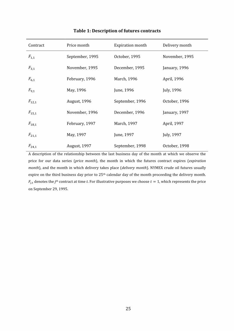
curve including contracts 1, 3, 6, 9, 12, 15, 18, 21, and 24. NYMEX crude oil futures

usually expire on the third business day prior to the 25th calendar day of the

month preceding the delivery month. The delivery month for contract 1 is the one

that follows its expiration month. Contract 3 is for the third delivery month after

contract 1. Contracts 6 to 24 are then analogously defined.

15

Table 1 summarises the relationship between the price of contract j at ,

month of expiration, and month during which the delivery takes place.

[Table 1 around here]

The same logic applies as is varied. For the empirical analysis, a monthly series of

200 observations was constructed using the closing prices on the last business day

of each month 1996M09-2012M04. This avoids concerns about roll-over strategy

and calendar effects. We denote the price of the jth contract at time as , so that

represents the price of contract 1 at month .

Table 2 provides descriptive statistics for two non-overlapping subsamples,

one up to the end of 2003 and the other commencing in January 2004.

[Table 2 around here]

The break point was chosen to highlight the effect of increased investment flows

in commodities since 2004. The post-2004 standard deviation is almost the same

for each series. Short-dated contracts are positively skewed but, as we move

towards more distant contracts, the skewness lessens and becomes even negative

for contracts 18, 21, and 24. The kurtosis for all contracts stays within the range of

a normally distributed variable.The table reveals some interesting patterns.

Overall, oil spot and futures price dynamics changed significantly after 2004.

Prices remained in a very narrow range during 1995-2003 in comparison to the

2004-2012 period when the maximum price for all contracts was close to $140

per barrel or virtually double the mean prices. The latter reached an all-time high

in 2008 followed by a sharp collapse. The post-2004 mean prices and standard

deviations increased three to four times in comparison with their corresponding

figures for pre-2004 period. The above factors point to distinct investor behaviour

in the post-2004 period. For example, Büyükşahin et al. (2009) show that the growth

16

of large net positions in long-dated contracts by hedge funds and other investors dates

from 2004 and 2005.

Prior to 2004 the mean price and mean standard deviation decrease as we

move towards longer dated contracts. At the same time the mass of the

distribution shifts from right to the left and becomes more platykurtic. After 2004

we observe that the mean price increases up to contract 9 and then flattens out or

decreases marginally. This can be seen more clearly in Figure 1 which plots the

average return of all contracts at different maturities over the two periods.

[Figure 1 around here]

Figure 1 can be viewed as an average term structure or yield curve for futures

prices over the two periods. Interestingly the 2004 break coincides with that

identified in Büyükşahin et al. (2009) for the nearby contract basis. The downward

sloping futures yield curve in panel A implies that the crude oil futures market was

backwardated prior to 2004. A trader with a long futures position on average

would realize a positive return from rolling her position forward into the cheaper

(next) nearby contract. By contrast, panel B show that that the futures yield curve

switched to contango with a positive slope in the period from 2004. Now contracts

further out the curve cost more and so rolling a nearby position to the next

contract would on average be more costly. Moreover a contangoed market may

encourage investors to buy longer maturity contracts to avoid rollover risk.

6 Empirical results

The power of the and

tests deteriorates if the bubble bursts within

the sample period. Homm and Breitung (2012) suggested that successive

observations following the explosive period are excluded from the sample to

overcome this problem. The spectacular downturn in the price of oil since June

17

2008 bears a close resemblance to a collapsing bubble. Therefore, the and

statistics are estimated over the period 1995M09:2008M06. The

and

statistics are obtained from the whole sample.

The recursive regressions were run with an initial window size of 36

observations (18% of the total sample) due to the small sample size. The test

results are given in Panel A of Table 3 while Panel B provides various right-side

critical values.

[Table 3 around here]

An analysis of the results in the Table 3 leads to several conclusions. First, all

statistics for the spot price series readily reject the null hypothesis of no bubbles

at the 1% level. Second, all statistics for all of the futures price series also provide

evidence against the null hypothesis of no bubble the 1% level. This result is novel

and is one of the original findings of this study. Finally, the evidence supporting

bubbles becomes stronger as the maturity of futures contracts increases.

While Table 3 provides strong evidence of bubbles, we next need to date

stamp them. Table 4 present the results from the Phillips, Shi, and Yu (2012) GSDF

procedure on bubble origination and collapse dates. The GSDF results are

presented first as this is the most general dating procedure in the presence of

multiple bubbles. We follow the literature in imposing a minimum six month

bubble duration period. Shorter episodes are regarded as blips.

[Table 4 around here]

There are some striking patterns in the results. First, they indicate no bubble in

spot prices and the nearby futures (contract 1) at the 5% significance level. The

identical results for the spot and nearby contracts are no surprise as otherwise

18

there would have been arbitrage opportunities. They are in line with long standing

results that the spot and nearby prices are cointegrated.

By contrast, the results point to a minimum six-month bubble period for

contacts 3 through to 24 with a collapse date of September 2008. The latter

coincides with that found in Phillips and Yu (2011), and Shi and Arora (2012).

Second, the bubble duration increases along the yield curve. For example, it ranges

from just 6 months (February to August 2008) for contract 3 to some four and a

half years for contract 24 at the 5% level. Contracts 6 through to 18 exhibit

evidence of multiple bubbles but there is a continuous bubble for contracts 21 and

24 from March 2004 to August/September 2008 at the 5% level.

The contrasting results between the spot (and nearby) and longer dated futures

contracts at the 5% level points to a fundamental disconnect in the crude oil

market. This in turn suggests a violation of market efficiency in the 2004-08

period. Market efficiency would imply cointegration between spot and longer

dated futures contracts which require both series to have a similar order of

integration. Our results contrast with those of Büyükşahin et al. (2009). Their ADF

test results for the period from July 2000 to August 2008 showed that nearby, 1- and 2-

year futures prices were all I(1) and their cointegration results indicated the prices were

cointegrated with one cointegrating vector. One possible explanation is the following.

A well-known limitation of Dickey-Fuller type tests is that when the data are

described by the generating process in Equation (9) with a coefficient close to but

different from one, the unit root null hypothesis cannot be properly assessed.

Finally, there is strong evidence of the bubble commencing in early 2004 for

longer maturity contracts. Contracts 15, 18, 21 and 24 show evidence of multiple

and continuous bubbles at the 5% level starting in early 2004 while, at the 10%

19

level, contracts 12 to 24 show evidence of a continuous bubble starting in early

2004. Interestingly, the year 2004 marks the increase of investment flows into

commodity derivatives market that many researchers believe changed oil futures

price behaviour (see, e.g., Sockin and Xiong (2013), Tang and Xiong (2012), and

Singleton (2012)). In that sense, the bubble duration evidence from the GSDF

detector for the longer maturity contracts is consistent with the financialisation of

commodities hypothesis.

Table 5 present the results from the FLUC procedure on bubble origination

and collapse dates.

[Table 5 around here]

The results exhibit the same broad patterns found using the GSDF procedure. The

only difference between the results in Tables 4 and 5 that the GSDF test results

indicate the bubble origination date to be earlier than the FLUC date for contacts

15 to 24 at the 5% level. Such differences in results may emerge for several

reasons. First, when there are multiple episodes of mildly explosive behaviour in

the data series (as in contracts 15 through to 18 at the 5% level), the GSDF

procedure consistently estimates the origination and end dates for each of them

(see Theorems 3, 4 and 5 in Phillips, Shi, and Yu (2012)). Second, the FLUC

detector uses a critical boundary that expands with each observation over the

range ⌊ ⌋ . In the case of a single period of mildly explosive behaviour, FLUC

may be considered a more conservative procedure so that stronger evidence

would be required to reject the null hypothesis.

The bubble periods detected by the CUSUM procedure are presented in

Table 6.

[Table 6 around here]

20

In contrast to the GSDF and FLUC procedures, the CUSUM test provides evidence

at the 5% level of bubbles in the spot and nearby contracts. The results similarly

show evidence of continuous bubbles from early 2004 to August/ September 2008

in contracts 15 to 24. These results are interesting since Phillips, Shi, and Yu

(2012) argued that CUSUM is a conservative procedure in comparison to their

strategy. In our application it identified more extensive periods of explosiveness

than the GSDF algorithm.

To sum up, both the GSADF and FLUC data stamping results indicate a

disconnect between the spot and nearby contracts on one hand and the longer

dated futures contracts on the other hand. The date stamping strategies identified

that the bubble origination date for more distant futures contracts is significantly

earlier than that for spot prices and contracts with shorter maturity. The upshot is

that there is a clear indication that futures contracts with maturity above six

months have been traded at prices considerably higher than their fundamental

level since early 2004. This sparks the question of what caused the bubble.

One of the most significant changes in the commodity market behaviour

during the bubble that we document is the growth of institutional investors. More

details on the exact type of investor and their changing investment patterns are

provided in Büyükşahin and Robe (2013) and Büyükşahin et al. (2009). Figure 2

shows that the bubble period coincides with a sharp increase of trading in the

crude oil futures market. A large body of empirical work indicate that financial

institutions have a sizable effect on asset prices. In an asymmetric information

setting, Allen and Gorton (1993) provide a model in which a bubble arises in

rational expectation equilibrium because of institutional investors’ agency

21

problem. The portfolio manager’s payoff has the form of a call option, which will

induce them to speculate on the future asset price path.

6 Conclusions

This paper investigates the time-series properties of spot and futures crude oil

prices for the presence of mildly explosive bubbles. In particular, we have applied

a battery of novel tests of the unit root null against a mildly explosive alternative

to monthly data over the sample period September 1995 to April 2012. The

procedures employed allow for consistent identification of bubble origination and

collapse dates. It has examined time-series properties of the range of futures price

from the nearby contract right out to the 24-month contract.

The results are novel. Both the Phillips et al. (2012) GSADF and the Phillips

et al. (2011) FLUC data stamping results indicate a disconnect between the spot

and nearby contracts on one hand and the longer dated futures contracts on the

other hand. The former exhibit no evidence of bubbles while the latter provide

significant evidence of extensive bubble periods. They indicate that the prices for

6-month series and beyond series were above their intrinsic values and thus

exhibited bubble behaviour in the period up until late 2008. Strikingly, the bubble

period starts significantly earlier for longer dated contracts than in shorter-dated

contracts. Specifically, there is strong evidence of a prolonged bubble in both the

21- and 24-month futures prices from 2004 to 2008. The latter coincides with the

period of increased participation of financial investors including index trackers

and hedge funds in commodity derivative markets. Although a necessary

condition, our new results do not necessarily infer that excessive speculation in

commodity futures markets contributed towards price deviations away from

22

fundamental levels in the physical market. Further empirical analysis is needed to

clarify the potential source of bubble behaviour.

23

References

Abreu, D., and M.K. Brunnermeier, 2003, Bubbles and crashes, Econometrica 71,

173-204.

Allen, F., and G. Gorton, 1993, Churning bubbles, Review of Economic Studies 60,

813–836.

Blanchard, O. J., and M.W. Watson, 1982, Bubbles, rational expectations, and

financial markets, in P. Wachtel, ed., Crisis in the Economic and Financial

Structure, 295-315 (Lexington Books).

Buyuksahin, B., M. Haigh, J. Harris, J. Overdahl, and M. Robe, 2009, Fundamentals,

trader activity and derivative pricing. Paper presented at the 2009 Meeting of

the European Finance Association.

Buyuksahin, B. and M. Robe, 2013. Speculators, commodities and cross-market

linkages. Journal of International Money and Finance, Forthcoming.

Campbell, J.Y., and R.J. Shiller, 1987, Cointegration and tests of present value

models, Journal of Political Economy 95, 1062-1088.

Diba, B.T., and H.I. Grossman, 1988a, The theory of rational bubbles in stock prices,

Economic Journal 98, 746-754.

Diba, B.T., and H.I. Grossman, 1988b, Explosive rational bubbles in stock prices,

American Economic Review 78, 520-530.

Evans, G.W., 1991, Pitfalls in testing for explosive bubbles in asset prices, American

Economic Review 81, 922-930.

Fama, E.F., 1965, Behavior of stock-market prices, Journal of Business 38, 34-105.

Homm, U., and J. Breitung, 2012, Testing for speculative bubbles in stock markets:

A comparison of alternative methods, Journal of Financial Econometrics 10, 198-

231.

Masters, M.W., 2008, Testimony before the US Senate Committee of Homeland

Security and Government Aairs, Washington (DC), May 20.

Jarrow, R.A., and P. Protter, 2009, Forward and futures prices with bubbles,

International Journal of Theoretical and Applied Finance 12, 901-924.

Phillips, P.C.B., and T. Magdalinos, 2007a, Limit theory for moderate deviations

from unit root, Journal of Economics 136, 115-130.

24

Phillips, P.C.B., and T. Magdalinos, 2007b, Limit theory for moderate deviations

from unity under weak dependence, in G.D.A. Phillips, and E. Tzavalis, eds., The

refinement of econometric estimation and test procedures: Finite sample and

asymptotic analysis, 123-162 (Cambridge University Press).

Phillips, P.C.B., S P. Shi, and J. Yu, 2012, Testing for multiple bubbles, Yale

University, Cowles Foundation Discussion Paper, No. 1843.

Phillips, P.C.B., Y. Wu, and J. Yu, 2011, Explosive behavior in the 1990s Nasdaq:

When did exuberance escalate asset values, International Economic Review 52,

201-226.

Phillips, P.C.B., and J. Yu, 2011, Dating the timeline of financial bubbles during the

subprime crisis, Quantitative Economics 2, 455-491.

Said, S.E., and D.A. Dickey, 1984, Testing for unit roots in autoregressive-moving

average models of unknown order, Biometrika 71, 599-607.

Shi, S., and V. Arora, 2012, An application of a model of speculative behaviour to oil

prices, Economics letters 115, 469-472.

Singleton, K.J., 2012, Investor flows and the 2008 boom/bust in oil prices, Stanford

University, Working paper.

Sockin, M., and W. Xiong, 2013, Informational frictions and commodity markets,

Princeton University, Working paper.

Soros, G., 2008, Testimony before the US Senate Commerce Committee Oversight

Hearing on FTC Advanced Rulemaking on Oil Market Manipulation, Washington

(DC), June 4.

Tang, K., and W. Xiong, 2012, Index investment and financialization of

commodities, Financial Analysts Journal 68, 54-74.

US Senate Permanent Subcommittee on Investigations, 2006, The role of market

speculation in rising oil and gas prices: A need to put the cop back on the beat,

Washington (DC), June 27.

25

Table 1: Description of futures contracts

Contract Price month Expiration month Delivery month

September, 1995 October, 1995 November, 1995

November, 1995 December, 1995 January, 1996

February, 1996 March, 1996 April, 1996

May, 1996 June, 1996 July, 1996

August, 1996 September, 1996 October, 1996

November, 1996 December, 1996 January, 1997

February, 1997 March, 1997 April, 1997

May, 1997 June, 1997 July, 1997

August, 1997 September, 1998 October, 1998

A description of the relationship between the last business day of the month at which we observe the

price for our data series (price month), the month in which the futures contract expires (expiration

month), and the month in which delivery takes place (delivery month). NYMEX crude oil futures usually

expire on the third business day prior to 25th calendar day of the month proceeding the delivery month.

denotes the jth contract at time t. For illustrative purposes we choose , which represents the price

on September 29, 1995.

26

Table 2: Descriptive statistics

Spot Contract 1 Contract 3 Contract 6 Contract 9 Contract 12 Contract 15 Contract 18 Contract 21 Contract 24

Panel A: Period 1995M09 to 2003M12 (100 observations)

Mean 23.389 23.368 22.866 22.208 21.681 21.269 20.941 20.703 20.537 20.422

Median 23.345 23.390 22.830 21.660 20.710 20.535 20.215 20.205 20.035 19.915

Maximum 36.760 36.600 33.280 30.300 29.160 28.450 27.900 27.470 27.130 26.920

Minimum 11.370 11.220 12.140 12.830 13.140 13.410 13.620 13.860 14.070 14.260

Std. Dev. 5.862 5.872 5.335 4.693 4.214 3.842 3.536 3.291 3.100 2.957

Skewness 2.148 2.149 2.009 1.916 1.878 1.842 1.822 1.823 1.834 1.864

Kurtosis -0.019 -0.026 -0.053 -0.045 -0.019 0.011 0.034 0.056 0.088 0.131

Panel B: Period 2004M01 to 2012M04 (100 observations)

Mean 73.715 73.768 74.822 75.485 75.761 75.865 75.826 75.734 75.608 75.465

Median 70.945 70.985 72.430 74.050 74.545 75.275 75.595 75.240 74.740 74.270

Maximum 139.960 140.000 140.950 141.560 141.460 140.870 140.200 139.480 138.930 138.420

Minimum 33.160 33.050 31.490 30.080 29.300 28.700 28.210 27.770 27.430 27.220

Std. Dev. 22.706 22.715 22.534 22.588 22.646 22.669 22.630 22.612 22.608 22.593

Skewness 2.764 2.758 2.849 2.908 2.933 2.942 2.962 2.973 2.982 2.987

Kurtosis 0.416 0.415 0.357 0.266 0.183 0.107 0.043 -0.010 -0.054 -0.090

The main characteristics of monthly spot and futures price series are reported for two non-overlapping periods. Series are constructed using the closing WTI crude

oil prices on the last business day of the month. The delivery month for contract 1 is the month that follows after the expiration of the contract. Contracts 3 to 24

are the successive delivery months following contract 1. NYMEX crude oil futures expire on the third business day prior to 25th calendar day of the month

proceeding the delivery month. If 25th happens to be a non-business day, the expiration day is the third business day prior to the business day proceeding 25th.

27

Table 3: Testing for explosive behaviour in WTI crude oil spot and futures price

series

SDF SDFC

SBT GSDF

Panel A: Test statistics

Spot 4.233 4.734 8.727 4.233

Contract 1 4.203 4.705 8.636 4.203

Contract 3 4.664 5.147 9.723 4.664

Contract 6 5.182 5.659 10.988 5.182

Contract 9 5.537 6.019 11.836 5.537

Contract 12 5.770 6.258 12.373 5.770

Contract 15 5.924 6.414 12.720 5.924

Contract 18 6.034 6.530 12.977 6.034

Contract 21 6.131 6.634 13.231 6.131

Contract 24 6.195 6.704 13.418 6.195

Panel B: Critical values

90% 2.223 1.395 1.755 2.869

95% 2.587 1.749 2.284 3.196

99% 3.314 2.490 3.492 3.893

The and

test statistics are estimated over the horizon September 1995 to June 2008 (154

monthly observations) to enhance the power of the tests. The and

test statistics are

estimated over the horizon September 1995 to April 2012 (200 monthly observations). They are

calculated recursively with a fraction of the total sample (36 observations) for initial window

size. The right-side critical values in Panel B are approximated using Monte Carlo simulations with 10,000

replications.

28

Table 4: Bubble origination and collapse dates: GSDF results

Level of significance

10% 5%

Spot

2008M02 : 2008M08

-

Contract 1

2008M02 : 2008M08

-

Contract 3

2007M12 : 2008M08

2008M02 : 2008M07

Contract 6

2005M02 : 2006M08

2007M09 : 2008M08

2006M03 : 2006M08

2007M12 : 2008M08

Contract 9

2005M01 : 2006M11

2007M09 : 2008M08

2005M02 : 2006M08

2007M10 : 2008M08

Contract 12

2004M05 : 2008M08

2005M02 : 2006M08

2007M10 : 2008M08

Contract 15

2004M03 : 2008M08

2004M05 : 2006M11

2007M09 : 2008M08

Contract 18

2004M02 : 2008M08

2004M04 : 2006M12

2007M09 : 2008M08

Contract 21

2004M02 : 2008M09

2004M04 : 2008M08

Contract 24

2004M02 : 2008M09

2004M03 : 2008M09

The dating of the bubble periods are defined according to Equations (21). The initial sample for the GSDF

procedure is chosen to be around 18% of the total sample (36 observations). The estimations are done

over the horizon 1995M09:2012M04.

29

Table 5: Bubble origination and collapse dates: FLUC results

The dating of the bubble periods are defined according to Equations (18) and (19). The initial sample for

the FLUC procedure is chosen to be around 18% of the total sample (36 observations). The estimations

are done over the horizon 1995M09:2012M04.

Level of significance

10% 5%

Spot

2008M02 : 2008M07

-

Contract 1

2008M02 : 2008M07

-

Contract 3

2008M02 : 2008M08

2008M02 : 2008M07

Contract 6

2005M12 : 2006M08

2007M10 : 2008M08

2006M03 : 2006M08

2007M12 : 2008M08

Contract 9

2005M02 : 2006M08

2007M09 : 2008M08

2005M02 : 2006M08

2007M10 : 2008M08

Contract 12

2004M07 : 2006M11

2007M09 : 2008M08

2005M02 : 2006M08

2007M10 : 2008M08

Contract 15

2004M07 : 2008M08

2004M07 : 2006M11

2007M10 : 2008M08

Contract 18

2004M05 : 2008M08

2004M07 : 2006M12

2007M10 : 2008M08

Contract 21

2004M05 : 2008M08

2004M07 : 2008M08

Contract 24

2004M05 : 2008M09

2004M07 : 2008M08

30

Table 6: Bubble origination and collapse dates: CUSUM results

Level of significance

10% 5%

Spot

2007M10 : 2008M08

2008M02 : 2008M07

Contract 1

2007M10 : 2008M08

2008M02 : 2008M07

Contract 3

2006M03 : 2006M08

2007M09 : 2008M08

2007M12 : 2008M08

Contract 6

2005M01 : 2008M08

2005M12 : 2006M08

2007M10 : 2008M08

Contract 9

2004M07 : 2008M09

2005M02 : 2006M11

2007M09 : 2008M08

Contract 12

2004M05 : 2008M09

2005M01 : 2008M08

Contract 15

2004M04 : 2008M09

2004M05 : 2008M08

Contract 18

2004M03 : 2008M09

2004M05 : 2008M08

Contract 21

2004M03 : 2008M09

2004M05 : 2008M08

Contract 24

2004M03 : 2008M09

2004M05 : 2008M09

The dating of the bubble periods are defined according to Equations (18) and (19). The initial sample for

the CUSUM procedure is chosen to be around 18% of the total sample (36 observations). The estimations

are done over the horizon 1995M09:2012M04.

31

Figure 1: Futures curve

Panel A. Period 1995M09 to 2003M12

Panel B. Period 2004M01 to 2012M04

73

74

75

76

77

1 3 6 9 12 15 18 21 24

Ave

rage

Pri

ce

Contract Maturity

18

20

22

24

1 3 6 9 12 15 18 21 24

Ave

rage

Pri

ce

Contract Maturity

32

Figure 2: Trading volume

Time series (solid line) are the 12 month moving average of WTI futures volume. The volume is the

number of all trading contracts. The shaded area is the bubble period defined by the date-stamping

strategies for the long maturity contracts.

0

20

40

60

80

100

120

96 98 00 02 04 06 08 10 12

Bubble origination: 2004M05

Bubble collapse: 2008M09