b-splines - uliege · 3 computer aided design b-splines isaac j. schoenberg (1946) carl de boor...

1

Computer Aided Design

B-Splines

2


B-Splines

Three useful references :

R. Bartels, J.C. Beatty, B. A. Barsky, An introduction to Splines for use in Computer Graphics and Geometric Modeling, Morgan Kaufmann Publications,1987

JC.Léon, Modélisation et construction de surfaces pour la CFAO, Hermes, 1991

L. Piegl, W. Tiller, The NURBS Book, Second Edition, Springer , 1996

3


B-Splines

Isaac J. Schoenberg (1946) Carl De Boor (1972-76) Maurice G. Cox (1972) Richard Riesenfeld (1973) Wolfgang Boehm (1980)

4


B-Splines

For Bézier curves, the polynomial degree is directly related to the number of control points.

The control of the continuity between Bézier curves is not trivial

B-Splines are a generalization in the sense that the degree doesn't depend on the number of control points

One can impose every continuity at any point of the curve (we will see later how to do that)

They are polynomial curves, by pieces (Bézier curves have a unique polynomial representation along the interval of definition)

They may provide local control The parametrization can be freely chosen (with Bézier, it is fixed ,

usually 0<u<1. )

5


B-Splines

Basis of Bézier curves :

The support of the basis functions is the interval [0..1] Continuity is , and between different Bézier curves

it is enforced by a wise choice of the Pi 's

B-splines basis

The basis functions Nid are piecewise polynomials

Have a compact support + satisfy partition of the unity The continuity is defined at the basis function's level.

P u=∑i=0

d

Pi Bidu

P u=∑i=0

n

Pi N idu

C∞

6


B-Splines

B-spline basis functions Defined by the nodal sequence and by the

polynomials degree of the curve (d) There are n+1 such functions, indexed from 0 to n .

Nodal sequence: It is a series of values u

i (knots) of the parameter u of

the curve, not strictly increasing – there can be equal values.

There are m+1 such knots, indexed from 0 to m e.g. U={0, 1, 2, 3, 4, 5, 6, 7, 8, 9}

U={0, 0, 0, 1, 2, 3, 4, 5, 5, 5} U={0, 0, 0, 1, 2, 2, 3, 4, 4, 4}

7


B-Splines

Construction of B-Spline basis functions Truncated Power Function

It is a function of Cd-1 continuity

(u−ui)+d={(u−ui)

d if u≥ui

0 otherwiseu

i

8


B-Splines

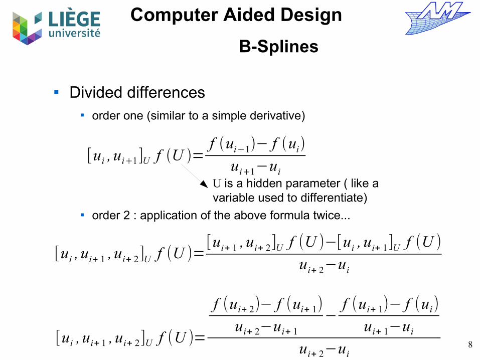
Divided differences order one (similar to a simple derivative)

order 2 : application of the above formula twice...

[ui , ui1]U f U =f ui1− f ui

ui1−uiU is a hidden parameter ( like a variable used to differentiate)

[ui , ui+ 1 , ui+ 2]U f (U )=[ui+ 1 , ui+ 2]U f (U )−[ui , ui+ 1]U f (U )

ui+ 2−ui

[ui , ui+ 1 , ui+ 2]U f (U )=

f (ui+ 2)− f (ui+ 1)

ui+ 2−ui+ 1

−f (ui+ 1)− f (ui)

ui+ 1−ui

ui+ 2−ui

9


B-Splines

At the order k

One assumed that

Properties (see Bartels, 1987)1- In the case where

2- if and

[ui ,⋯ , ui+k ] f =[ui+1 ,⋯ , ui+k ] f −[ui ,⋯ , ui+k−1] f

ui+k−ui

ui≠ui1≠ui2⋯

ui=ui1=ui2⋯

[ui ,⋯ , uik ] f =1k !

d k f

d uk ∣u=u i

ui≠ui+ 1≠ui+ 2⋯ uiui1ui2⋯

[ui ,⋯ , uik ] f =1k !

d k f

d uk ∣u=u*

, uiu*uik

10


B-Splines

3- is symmetric with respect to the knot vector

4- If f(u) is a polynomial of degree at the most equal to k , then

is a constant with respect to the ui.

5- The divided difference of f=g(u).h(u) is :

[ui ,⋯ , ui+ k ] f

[ui ,⋯ , ui+ k ] f

[ui ,⋯ , uik ] f = ∑j=i

j=ik

[ui ,⋯ , u j ] g ⋅[u j ,⋯ , uik ]h

11


B-Splines

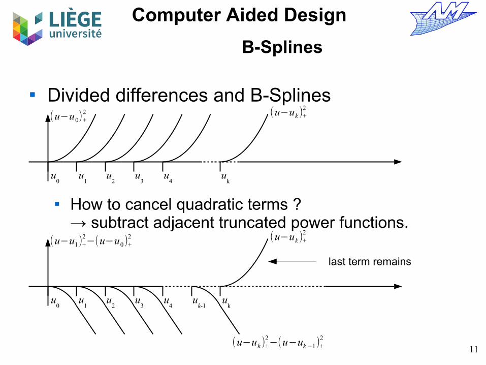
Divided differences and B-Splines

How to cancel quadratic terms ?→ subtract adjacent truncated power functions.

(u−u0)+2

u0

u1

u2

u3

u4

uk

(u−uk )+2

(u−u1)+2−(u−u0)+

2

u0

u1

u2

u3

u4

uk

(u−uk )+2

(u−uk )+2−(u−uk−1)+

2

uk-1

last term remains

12


B-Splines

Problem, lower order terms are dependent on k

But, dividing by yields a divided difference :

(u−uk )+2−(u−uk−1)+

2

uk−uk−1

=[uk−1 , uk ]U (u−U )+2

(uk−uk−1)

(u−uk)+2−(u−uk−1)+

2∣u>uk=0⋅u2

+(uk−uk−1)⋅u+(uk−uk−1)(uk+uk−1)⋅1

u0

u1

u2

u3

u4

uk

(u−uk )+2

uk-1

last term remains

[uk−1 , uk ]U (u−U )+2

[u0 , u1 ]U (u−U )+2

13


B-Splines

Now, cancel linear terms …

Same procedure : subtract adjacent terms.

u0

u1

u2

u3

u4

uk

(u−uk )+2

uk-1

last term remains

[uk−1 , uk ]U (u−U )+2

[u0 , u1 ]U (u−U )+2

u0

u1

u2

u3

u4

uk

(u−uk )+2

uk-1

Two last term remains

[uk−1 , uk ]U (u−U )+2

[u1 , u2 ]U (u−U )+2− [u0 , u1 ]U (u−U )+

2

14


B-Splines

Again, lower order terms are dependent on k

Dividing by yields a divided difference again :

[uk−1 , uk−2 ]U (u−U )+2− [uk , uk−1 ]U (u−U )+

2

uk−uk−2

=[uk−2 , uk−1 , uk ]U (u−U )+2

(uk−uk−2)

[uk−1 , uk−2 ]U (u−U )+2− [uk , uk−1 ]U (u−U )+

2∣u>uk

=0⋅u+((uk+uk−1)−(uk−1+uk−2))⋅1=(uk−uk−2)⋅1

u0

u1

u2

u3

u4

uk

(u−uk )+2

uk-1


[uk−1 , uk ]U (u−U )+2

[u0 , u1 ,u2]U (u−U )+2

15


B-Splines

Now, cancel constant terms …

Same procedure : subtract adjacent terms.

u0

u1

u2

u3

uk-2

uk

(u−uk )+2

uk-1

Three last term remains

[uk−1 , uk ]U (u−U )+2

[u1 , u2 ,u3 ]U (u−U )+2− [u0 , u1 , u2 ]U (u−U )+

2

u0

u1

u2

u3

u4

uk

(u−uk )+2

uk-1


[uk−1 , uk ]U (u−U )+2

[u0 , u1 ,u2]U (u−U )+2

16


B-Splines

There are no lower order terms. However we might divide anyway by to remain consistent and get an expression as a divided difference again...

[uk−2 , uk−1 , uk ]U (u−U )+2−[uk−3 , uk−2 , uk−1 ]U (u−U )+

2

uk−uk−3

=[uk−3 , uk−2 , uk−1 , uk ]U (u−U )+2

(uk−uk−3)

u0

u1

u2

u3

uk-2

uk

(u−uk )+2

uk-1

Three last term remainthat will be discarded !

[uk−1 , uk ]U (u−U )+2

[u0 , u1 ,u2 , u3]U (u−U )+2 [uk−2 , uk−1 , uk ]U (u−U )+

2

17


B-Splines

The sign is alternating with the degree. Shape functions of even degree are negative, while SFs of uneven degree are positive.

Multiplying by makes every SF positive. To ensure that the SF form a partition of unity , we

have to multiply again by The compact representation of the B-Splines basis

functions of degree d with the use of divided differences is therefore :

(−1)d +1

N id=(−1)d+1

(ui+d+1−ui)[ui ,⋯ , ui+d+1]U (u−U )+d

(ui+d +1−ui)

18


B-Splines

u0

u1

u2

u3

uk-2

uk

uk-1

N id=(−1)d+1

(ui+d+1−ui)[ui ,⋯ , ui+d +1]U (u−U )+d

19


B-Splines

Proof of the partition of unity : consider the before last operation (the cancellation of constant terms)

We subtract consecutive terms to form the final shape functions Partition of unity means the sum of all the final shape functions is

equal to 1… that this is indeed the case only on a certain range of u.

u0

u1

u2

u3

u4

um-2

um-3

[um−2⋯um]U (u−U )+d

+-+

-+

-+

-...

um-1

um

1

More generally, there is partition of unity for , m+1 being the number of knots in the knot vector

ud≤u≤um−d

[u0⋯um]

K [um−d−1⋯um ]U (u−U )+d≡N m−d−1

d(u)N 0

d(u)

20


B-Splines

Recurrence relations It is easy to see that Replacing in

and using the expression of divided differences of a

product, it yields :

because DD of order >1 of (U–u)=0 . It simplifies to :

(u−U )+d=(u−U )(u−U )+

d−1

N id=(−1)d+1

(ui+d+1−ui)[ui ,⋯ , ui+d +1]U (u−U )+d

[ui ,⋯ , ui+k ] g⋅h= ∑j=i

j=i+k

([ui ,⋯, u j ] g )⋅([u j ,⋯ , ui+k ]h)

N id=(−1)d+1

(ui+d+1−ui) ([ui]U (u−U )[ui ,⋯ , ui+d +1]U (u−U )+d−1

+

[ui , ui+1]U (u−U )[ui+1 ,⋯, ui+d+1]U (u−U )+d−1 )

N id=(−1)(d+1)

(ui+d+1−ui) ((u−ui)[ui ,⋯ , ui+d+1]U (u−U )+d−1

+

(−1)[ui+1 ,⋯ , ui+d +1]U (u−U )+d−1 )

21


B-Splines

Using the recursive definition of the divided differences

one gets :

which is, to a term depending on the knot vector and

u, equal to .

N id=(−1)d

(u−ui)[ui ,⋯ , ui+d ]U (u−U )+d−1

+

(−1)d(ui+d+1−u)[ui+1 ,⋯ , ui+d +1]U (u−U )+

d−1

N id=

u−ui

ui+d−ui

N id−1

+ui+d +1−u

ui+d +1−ui+1

N i+1d−1

[ui ,⋯, ui+d+1] f =[ui+1 ,⋯, ui+d +1] f −[ui ,⋯ , ui+d ] f

ui+d +1−ui

N id=(−1)(d+1)

(ui+d +1−ui) ((u−ui)[ui ,⋯ , ui+d+1]U (u−U )+d−1

+

(−1)[ui+1 ,⋯ , ui+d+1]U (u−U )+d−1 )

22


B-Splines

Recursive definition of basis functions Setting

(nodal sequence) The functions are such as : (recurrence formula of

Cox – de Boor)

Where ui+d

– ui = 0, necessarily

By convention, we set in this case when the limit is undefined.

U={u0 ,⋯ , um} , ui≤ui1 , i=0⋯m−1

N idu=

u−ui

uid−ui

N id−1

u uid1−u

uid1−ui1

N i1d−1

u

N i0(u)={1 if ui≤u< ui+ 1

0 otherwise

00=0

N id−1

u ≡0

23


B-Splines

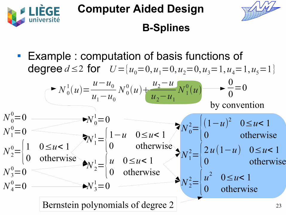
Example : computation of basis functions of degree for U={u0=0,u1=0,u2=0,u3=1,u4=1,u5=1}

N 00=0

N 10=0

N 20={1 0≤u< 1

0 otherwise

N 30=0

N 40=0

d≤2

N 01=0

N 11={1−u 0≤u< 1

0 otherwise

N 21={u 0≤u< 1

0 otherwise

N 31=0

N 02={(1−u)2 0≤u< 1

0 otherwise

N 12={2 u (1−u) 0≤u< 1

0 otherwise

N 22={u2 0≤u< 1

0 otherwise

Bernstein polynomials of degree 2

N 01u=

u−u0

u1−u0

N 00u

u2−u

u2−u1

N 10u

00=0

by convention

24


B-Splines

The Bernstein polynomials of degree d are a particular case of the B-splines basis

They correspond to a nodal sequence

Bézier curves are therefore a particular case of B-splines.

It is also possible to transform any B-spline into a sequence of Bézier curves – because the Bernstein polynomials form a complete basis of polynomials of degree d.

U B={u0=0,⋯ , ud=0,ud1=1,⋯ , u2 d1=1}

25


B-Splines

Basis functions and control points In contrary to Bézier curves, the number of control

points is not imposed by the degree d Let m+1 the number of knots. We have n+1

independent basis functions at our hands For every basis function, we associate a control point

The number of control points is fixed by the relation n+1=m-d

P u=∑i=0

n

Pi N idu

26


B-Splines

Types of nodal sequence... Uniform – The gap between two successive knots is constant

Periodic - The gap between the knots at the start of a nodal sequence is identical to the one at the end of the nodal sequence

Non uniform, interpolating – first and last control point are interpolated

In the sequel, except where indicated, we consider non uniform nodal sequences interpolating the first and last control points.

U={a ,⋯, ad1

, ud1 ,⋯ , um−d−1 , b ,⋯, bd1

}

U={u0 , u1 ,⋯ , um−d−1} , ui1−ui=k

U={u0,⋯ , udd1

, ud1 ,⋯, um−d−1 , u ' 0,⋯ , u ' dd1

} , u ' i−ui=k

27


B-Splines

U={0,56

,106

,156

,206

,256

,5} d=0 m1=7 n1=6

28


B-Splines

U={0 ,0 ,1 ,2 ,3 ,4 ,5 ,5} d=1 m1=8 n1=6

29


B-Splines

U={0 , 0 , 0 ,54

,104

,154

,5 , 5 ,5} d=2 m1=9 n1=6

30


B-Splines

U={0 , 0 , 0 ,0,53

,103

,5 , 5 ,5 ,5} d=3 m+1=10 n+1=6

31


B-Splines

U={0 , 0 , 0 ,0,0 ,52

, 5 ,5 ,5 ,5 ,5} d=4 m1=11 n1=6

32


B-Splines

U={0 , 0 , 0 ,0, 0 , 0 ,5,5 , 5 ,5 ,5 ,5} d=5 m1=12 n1=6Bernstein polynomials (with a factor on u)

33


B-Splines

Properties of B-spline basis functions outside the interval Inside the interval , at most d+1 functions

are non zero : (always positive) For (forms a partition of

unity) All derivatives of exist inside the

interval . At a knot , is d-k times differentiable, k being the node multiplicity.

Except for d=0, reaches exactly one maximum

N idu=0 [ ui , ui+d+1[

[ ui , ui+1 [N *

d(u) N i−d

d ,⋯ , N id

N id(u)≥0 ∀ i , d and u

u∈[ ui , ui+1 [ , ∑j=i−d

i

N jd(u)=1

N idu

[ ui , ui1 [ N idu

N idu

34


B-Splines

u0

u1

u2

u3

uk-2

uk

uk-1

N id=(−1)d+1

(ui+d+1−ui)[ui ,⋯ , ui+d +1]U (u−U )+d

35


B-Splines

U={0 , 0 ,0 ,0,1 , 2 ,3 ,4 ,5 ,5 ,5 ,5} d=3 m1=12 n1=8The knot u=3 is of multiplicity 1

36


B-Splines

U={0 , 0 , 0 ,0,1 , 2 ,3 ,3 ,5 ,5 , 5 ,5} d=3 m1=12 n1=8The node u=3 is of multiplicity 2

37


B-Splines

U={0 , 0 , 0 ,0,1 ,3 , 3 , 3 ,5 ,5 ,5 ,5} d=3 m1=12 n1=8The node u=3 is of multiplicity 3

38


B-Splines

U={0 , 0 , 0 ,0,3 ,3 ,3 , 3 ,5 ,5 ,5 ,5} d=3 m1=12 n1=8The node u=3 is of multiplicity 4

Curve 1 Curve 2

39


B-Splines

Derivatives of B-spline basis functions Definition by recurrence

k should not exceed d : every derivative of higher order vanish.

d k N id

d uk =N id ,k

=d N id−1,k−1

uid−ui

−N i1

d−1 ,k−1

uid1−ui1

40


B-Splines

The characteristics of basis functions involve that the B-Spline curve

interpolates P

0 and P

n , only if the nodal sequence

admits d+1 repetitions at the start and at the end ! is invariant by affine transformation , is contained by the convex hull of the control points

(because P(u) is a linear combination of the control points with positive coefficients which sum to one)

P u=∑i=0

n

Pi N idu U={u0 ,⋯ , um} , ui≤ui1 , i=0⋯m−1

41


B-Splines

(Following) Is variation diminishing : The number of inflexion

points is lower than the number of wiggles of the characteristic polygon

Is closed and convex if the characteristic polygon is closed and convex,

Is of length shorter or equal than that of the control polygon.

Is invariant by linear transformation of the nodal sequence u'=au+b , a>0

42


B-Splines

Control points, degree and nodal sequence We associate a control point for each basis function

Ni* . We have n+1 control points.

The degree d is chosen by the user. The nodal sequence (that defines the intervals of the

parameter on which the curve has a unique polynomial definition) is then built. We have m+1=n+d+2 knots (with d+1 repetitions at the start and at the end)

there remains n-d values of the parameter to set (without taking the boundaries into account)

43


B-Splines

Geometric examples Constant number of control points We increase the degree Uniform repartition of knots (except at boundaries) For which degree do we have the best approximation

of the control points ??

44


B-Splines

Degree 10 0 0.0833333 0.166667 0.25 0.333333 0.416667 0.5 0.583333 0.666667 0.75 0.833333 0.916667 1 1

45


B-Splines

degree 20 0 0 0.0909091 0.181818 0.272727 0.363636 0.454545 0.545455 0.636364 0.727273 0.818182 0.909091 1 1 1

46


B-Splines

degree 30 0 0 0 0.1 0.2 0.3 0.4 0.5 0.6 0.7 0.8 0.9 1 1 1 1

47


B-Splines

degree 40 0 0 0 0 0.111111 0.222222 0.333333 0.444444 0.555556 0.666667 0.777778 0.888889 1 1 1 1 1

48


B-Splines

degree 60 0 0 0 0 0 0 0.142857 0.285714 0.428571 0.571429 0.714286 0.857143 1 1 1 1 1 1 1

49


B-Splines

degree 100 0 0 0 0 0 0 0 0 0 0 0.333333 0.666667 1 1 1 1 1 1 1 1 1 1 1

50


B-Splines

degree 12 (Bézier)0 0 0 0 0 0 0 0 0 0 0 0 0 1 1 1 1 1 1 1 1 1 1 1 1 1

51


B-Splines

Impose interpolation points (and C0 continuity )

It is the same as positioning knots of multiplicity d in the nodal sequence

One could also repeat d control points...(not shown here)

52


B-Splines

degree 3 0 0 0 0 0.1 0.2 0.5 0.5 0.5 0.7 0.9 0.9 0.9 1 1 1 1

u=0

u=0.1

u=0.2

u=0.5

u=0.7

u=0.9

u=1

53


B-Splines

degree 3 (4 Bézier curves of continuity C0)

0 0 0 0 0.1 0.1 0.1 0.5 0.5 0.5 0.9 0.9 0.9 1 1 1 1

u=0.1

u=0.5u=0.9

u=0

u=1

54


B-Splines

degree 3 (3 Bézier curves of continuity C0 + 1 bspline deg 3 with 4control pts)

0 0 0 0 0.1 0.1 0.1 0.4 0.4 0.4 0.8 0.8 0.8 0.9 1 1 1 1

u=0.1

u=0.4u=0.8

u=0

u=1

u=0.9

55


B-Splines

And if we want to impose interpolation points and a certain continuity C

k ?

Add / align control points in a similar way than in the case of Bézier curves.

56


B-Splines

57


B-Splines

Periodic curves They may be represented by modifying the nodal

sequence and by repeating some control points.

Non-uniform nodal sequence

Uniform nodal sequence

uniform nodal sequenceand periodic curve

58


B-Splines

degree 3 0 0 0 0 0.1 0.2 0.3 0.4 0.5 0.6 0.7 0.8 0.9 1 1 1 1

non uniform nodal sequence interpolating the first and last control points.

59


B-Splines

degree 3 -0.3 -0.2 -0.1 0 0.1 0.2 0.3 0.4 0.5 0.6 0.7 0.8 0.9 1 1.1 1.2 1.3

Periodic nodal sequence(but control points located inadequately)

60


B-Splines

degree 3 -0.3 -0.2 -0.1 0 0.1 0.2 0.3 0.4 0.5 0.6 0.7 0.8 0.9 1 1.1 1.2 1.3

61


B-Splines

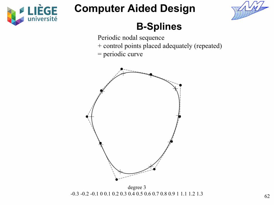
degree 3 -0.3 -0.2 -0.1 0 0.1 0.2 0.3 0.4 0.5 0.6 0.7 0.8 0.9 1 1.1 1.2 1.3

62


B-Splines

degree 3 -0.3 -0.2 -0.1 0 0.1 0.2 0.3 0.4 0.5 0.6 0.7 0.8 0.9 1 1.1 1.2 1.3

Periodic nodal sequence+ control points placed adequately (repeated)= periodic curve

63


B-Splines

Algorithms for the manipulation of B-Splines curves

Boehm's knot insertion algorithm Evaluation of the curve (Cox-de Boor algorithm) Derivatives and hodographs Restriction/growth of the useful interval of a curve Degree elevation Recursive Subdivision

64


B-Splines

Boehm's knot insertion algorithm

The idea is to determine a new control polygon for the same curve after the insertion of one or several knots in the nodal sequence.

The curve is not modified by this change : neither the shape nor the parametrization are affected.

Interest : Evaluation of points on the curve Subdivision of the curve Addition of control points

65


B-Splines

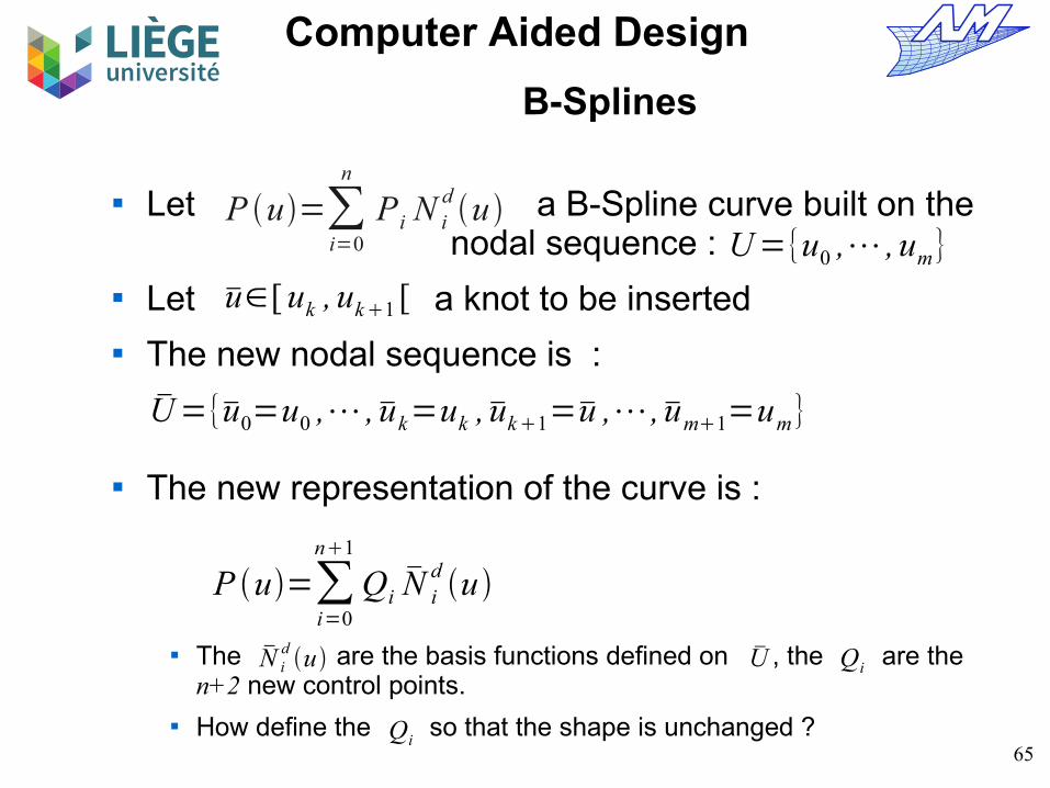
Let a B-Spline curve built on the nodal sequence :

Let a knot to be inserted The new nodal sequence is :

The new representation of the curve is :

The are the basis functions defined on , the are the n+2 new control points.

How define the so that the shape is unchanged ?

P u=∑i=0

n

Pi N idu

U={u0 ,⋯ , um}

u∈[ uk , uk1 [

U={u0=u0 ,⋯ ,uk=uk ,uk1=u ,⋯,um1=um}

P u=∑i=0

n1

QiN i

du

N idu U Qi

Qi

66


B-Splines

Let's set We write the relation for n+2 distinct values of u.

(a,b,... ) We obtain a band system, with 3(n+2) unknowns (in

3D)

It's costly to solve and it assumes that the values a,b.... are carefully set to avoid a singular lin. system

P (u)=∑i=0

n

Pi N id(u)=∑

i=0

n+ 1

Qi N id(u) ∀u

N 0

da N 1

da ⋯

N 0db N 1

db ⋯

⋮ ⋮ ⋱

Q0

Q1

⋮=

∑i=0

n

P i N ida

∑i=0

n

Pi N idb

⋮

67


B-Splines

Use of properties of basis functions We have . In this interval

, we have (compact support) In the same way,

and . Thus, we have :

For :

Proof using the definition of shape functions, see Leon's book p.333

u∈[ uk , uk+1[N i

d(u)≠0 iff i∈{k−d ,⋯, k }

N id(u)≠0 iff i∈{k−d ,⋯, k+1}

[ uk , uk+1[

P (u)= ∑i=k−d

k

P i N id(u)= ∑

i=k−d

k+1

Q i N id(u)

N id(u)= N i

d(u) for i∈{0 ,⋯ , k−d−1}

N id(u)= N i+1

d(u) for i∈{k+1 ,⋯ , n}

i∈{k−d ,⋯ , k }

N id(u)=

u−ui

ui+d+1−ui

N id(u)+

ui+d+2−u

ui+d+2−ui+1

N i+1d(u)

u∈[ uk , uk1 [

68


B-Splines

involves

involves

We substitute in

N id(u)= N i

d(u) for i∈{0 ,⋯ , k−d−1}

P i=Q i for i∈{0 ,⋯ , k−d−1}N i

d(u)= N i+1

d(u) for i∈{k+1 ,⋯ , n}

P i=Qi+ 1 for i∈{k+ 1 ,⋯, n}

N id(u)=

u−ui

ui+d+1−ui

N id(u)+

ui+d+2−u

ui+d+2−ui+1

N i+1d(u)

∑i=k−d

k

P i N id(u)= ∑

i=k−d

k+1

Qi N id(u)

69


B-Splines

(u−uk−d

uk+1−uk−d

N k−dd

(u)+uk +2−u

uk+2−uk−d+1

N k−d+1d

(u))Pk−d

+(u−uk−d+1

uk +2−uk−d +1

N k−d+1d

(u)+uk+3−u

uk +3−uk−d+2

N k−d+2d

(u))Pk−d+1

+⋯

+(u−uk

uk+d +1−uk

N kd(u)+

uk +d+2−u

uk +d+2−uk +1

N k+1d

(u))P k

= N k−dd

(u)Qk−d+⋯+ N k+1d

(u)Qk +1

N id(u)=

u− ui

ui+d+1−ui

N id(u)+

ui+d +2−u

ui+d +2− ui+1

N i+1d

(u) ∑i=k−d

k

P i N id(u)= ∑

i=k−d

k +1

Q i N id(u) in

70


B-Splines

By factoring and replacing the nodal sequence by U , we obtain :

We set

with

...

0= N k−dd

(u) (Qk−d−P k−d )

+ N k−d+1d

(u)(Q k−d +1−u−uk−d +1

uk +1−uk−d +1

P k−d +1−uk +1−u

uk +1−uk−d+1

P k−d )⋮

+ N kd(u)(Qk−

u−uk

uk +d−uk

Pk−uk+d−u

uk+d−uk

P k−1)+ N k +1d

(u) (Qk +1−P k )

U

αi=u−ui

ui+d−ui

1−αi=ui+d−u

ui+d−ui

i∈{k−d+1 ,⋯ , k }

71


B-Splines

... we obtain

We had :

so finally :

Qk−d=Pk−d

Q i=α i P i+(1−αi)P i−1 for i∈{k−d+1 ,⋯, k }Qk +1=P k

P i=Q i for i∈{0 ,⋯ , k−d−1}P i=Q i+1 for i∈{k+1 ,⋯, n}

Q i=α i P i+(1−αi)P i−1 with αi={1 i≤k−d

u−ui

ui+ p−ui

k−d+1≤i≤k

0 i≥k+1

72


B-Splines

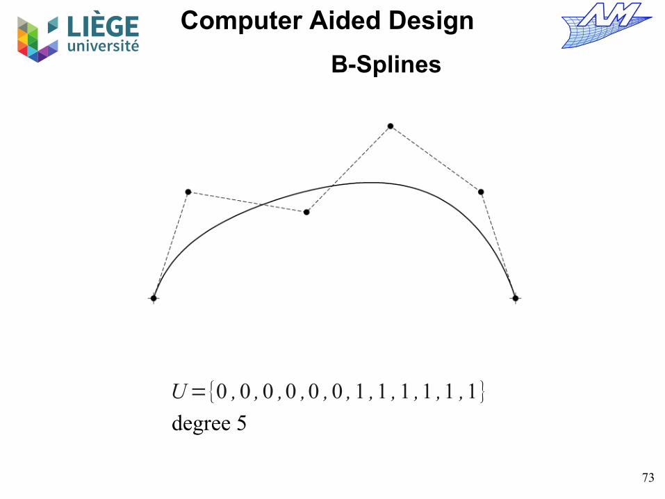
U={0 , 0 , 0 ,0 ,0 , 0 , 1 ,1 , 1 ,1 ,1 ,1}

degree 5

73


B-Splines

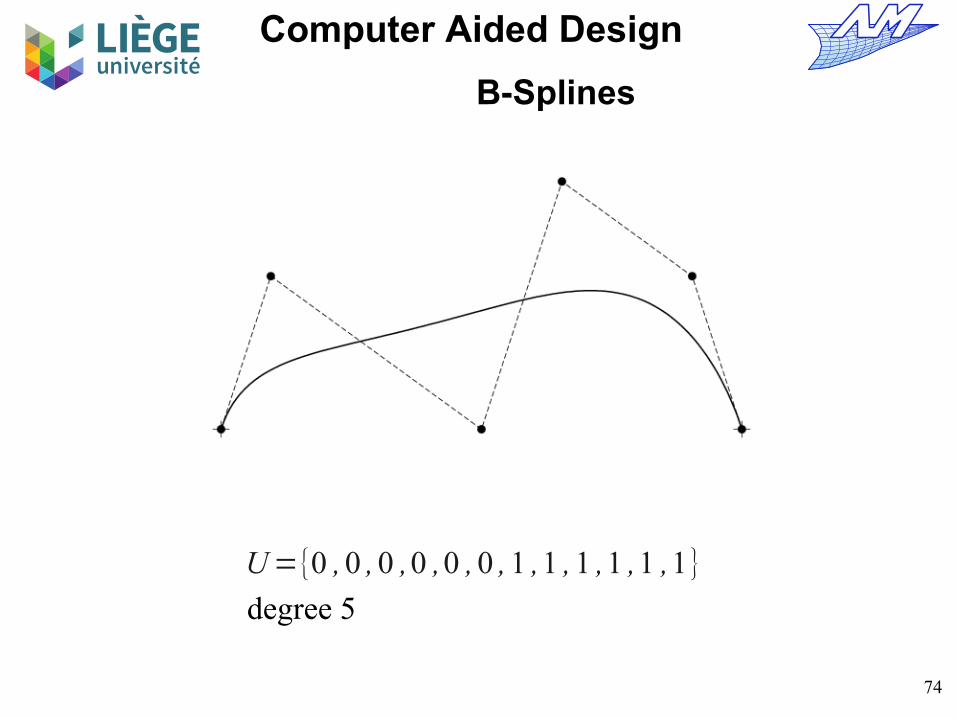
U={0 , 0 , 0 ,0 ,0 , 0 , 1 ,1 , 1 ,1 ,1 ,1}

degree 5

74


B-Splines

U={0 , 0 , 0 ,0 ,0 , 0 , 1 ,1 , 1 ,1 ,1 ,1}

degree 5

75


B-Splines

U={0 , 0 , 0 ,0 ,0 , 0 ,0.2 , 1 ,1 ,1 ,1 ,1 ,1}

degree 5

76


B-Splines

U={0 , 0 , 0 ,0 ,0 , 0 , 0.2 , 0.4 ,1 ,1 ,1 ,1 , 1 ,1}

degree 5

77


B-Splines

U={0 , 0 , 0 ,0 ,0 , 0 , 0.2 , 0.4 ,0.6 ,1 ,1 , 1 ,1 ,1 ,1}

degree 5

78


B-Splines

U={0 , 0 , 0 ,0 ,0 , 0 , 0.2 , 0.4 ,0.6 ,0.8 ,1 ,1 ,1 ,1 ,1 , 1}

degree 5

79


B-Splines

U={0 , 0 , 0 ,0 ,0 ,0 , 0.1 , 0.2 ,⋯ ,0.9 ,1 ,1 ,1 ,1 ,1 ,1}

degree 5

80


B-Splines

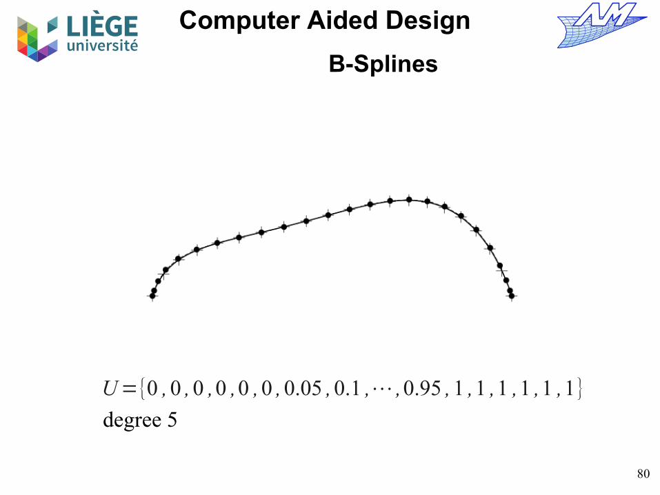
U={0 , 0 , 0 ,0 ,0 ,0 , 0.05 ,0.1 ,⋯ ,0.95 , 1 ,1 ,1 ,1 ,1 ,1}

degree 5

81


B-Splines

U={0 , 0 , 0 ,0 ,0 ,0 , 0.05 ,0.1 ,⋯ ,0.95 , 1 ,1 ,1 ,1 ,1 ,1}

degree 5Local control...

82


B-Splines

U={0 , 0 , 0 ,0 ,0 , 0 , 0.2 , 0.4 ,1 ,1 ,1 ,1 , 1 ,1}

degree 5

N id=(−1)d+1

(ui+d+1−ui)[ui ,⋯ , ui+d+1]U (u−U )+d

N idu=

u−ui

uid−ui

N id−1

uuid1−u

uid1−ui1

N i1d−1

u

N i0(u)={1 if ui≤u< ui+ 1

0 otherwise

83


B-Splines

Boehm’s knot insertion formula :

Q i=α i P i+(1−αi)P i−1 with αi={1 i≤k−d

u−ui

ui+ p−ui

k−d+1≤i≤k

0 i≥k+1

84


B-Splines

Multiple knot insertions Assume of multiplicity s ( ). We

want to insert it r times with .

We note Qir the control points of the r-th insertion step

We have then :

u∈[ uk , uk1 [rs≤d

0≤sd

Q ir=α i

r Q ir−1

+(1−αir)Q i−1

r−1 with αir={

1 i≤k−d+r−1u−ui

ui+d−r+1−ui

k−d+r≤i≤k−s

0 i≥k−s+1

85


Q k−d11

Qk−d22

Qk−d21

⋮ ⋮ ⋯ Q kd

Qk−11

Qk2

Qk1

B-Splines

The Q's can be put in a table:

The total number of new control points is d-s+r-1 that replace d-s-1.

P k−d

⋮

⋮

⋮

⋮

P k

86


B-Splines

The use of the algorithm of node insertion up to multiplicity of d=r+s is such that the curve will interpolate the last control point that is computed.

Therefore, one can use this algorithm to compute the position of a point of the curve knowing the parameter.

It's precisely the Cox-de Boor algorithm. The sequence of points Pij

is not anything else than the Qij indicated on the graph, cf following

Q k −d+11

Q k−d +22

Q k−d+21

⋮ ⋮ ⋯ Q kd

Qk−11

Q k2

Q k1

P k−d

⋮

⋮

⋮

⋮

Pk

87


B-Splines

Case r+s=d+1 : We carry out the insertion of multiplicity r-1 then we insert one more knot to « cut » the B-spline curve in two independent parts.

The last control point has to be duplicated. Allows to extract a portion of the B-spline.

There exists an extension of this algorithm in the case of the simultaneous insertion of many knots: it is the somewhat more complex “Oslo” algorithm* , not described here.

Qkd

* E. Cohen, T. Lyche, R. Riesenfeld “Discrete B-splines and subdivision techniques in computer-aided geometric design and computer graphics”, Computer Graphics and Image Processing, 14(2):87-111, 1980.

88


B-Splines

(simplified) Cox-de Boor Algorithm :

What is its complexity ? quadratic in function of the degree d.

Determine the interval of u : Initialization of For k from 1 to d For j from i-d+k to i

EndforEndfor is the point that is sought.

P jk=(

u−u j

u j+d +1−k−u j)P j

k−1+(

u j+d+1−k−u

u j+d+1−k−u j)P j−1

k−1

P id

P j0

u∈[ ui , ui+1 [i∈{d , d+1,⋯ ,m−d−1}

89


B-Splines

On a knot of multiplicity s :Determine the interval of u : Initialization of For k from 1 to d-s For j from i-d+k to i-s

EndforEndfor is the point that is sought.

P jk=(

u−u j

u j+d +1−k−u j)P j

k−1+(

u j+d+1−k−u


k−1

P i−sd−s

P j0

u∈[ ui−s=⋯=ui , ui+1 [and u=ui

i∈{d , d+1,⋯ , m−d−1}

90


B-Splines

Example of computation

Determination of the interval

Iteration 1

Iteration 2

Iteration 3

P00=(0 ,1) P1

0=(2 ,3) P2

0=(5 , 4) P3

0=(7 ,1) P4

0=(6 ,−1) P5

0=(6 ,−2)

U={0 , 0 ,0 ,0 ,1 , 2 , 3 , 3 ,3 ,3} d=3 u=3/2

1≤3/2<2 , u4=1 → i=4

P 41=(27/4 ,1 /2) P3

1=(6 ,5/2) P2

1=(17 /4 ,15/5)

P 42=(99 /16 , 2) P3

2=(89/16 , 45/16)

P 43=(47 /8 , 77 /32)=P (3/2)

P jk=(

u−u j

u j+d+1−k−u j)P j

k−1+(

u j+d+1−k−u


k−1

JC Leon

91


B-Splines

The algorithm is similar to De Casteljau's algorithm for Bézier curves

It is built on a restriction of the set of control points (d+1 points) On this restriction, it is nearly identical, except for the coefficients

related to the nodal sequence (which is potentially non uniform) The complete algorithm is somewhat longer than this one

(possibility to have 0/0 : we set conventionally 0/0 = 0 !)

92


B-Splines

U={0 , 0 , 0 ,0 ,0 , 0 , 1 ,1 , 1 ,1 ,1 ,1}

degree 5

93


B-Splines

U={0 , 0 , 0 ,0 ,0 , 0 ,0.3 ,1 ,1 ,1 ,1 ,1 , 1}

degree 5

94


B-Splines

U={0 ,0 , 0 ,0 ,0 , 0 , 0.3 , 0.3 ,1 , 1 ,1 ,1 ,1 ,1}

degree 5

95


B-Splines

U={0 , 0 , 0 ,0 ,0 , 0 , 0.3 , 0.3 ,0.3 ,1 ,1 ,1 ,1 , 1 ,1}

degree 5

96


B-Splines

U={0 , 0 , 0 ,0 ,0 ,0 , 0.3 , 0.3 ,0.3 ,0.3 , 1 ,1 ,1 ,1 ,1 ,1}

degree 5

97


B-Splines

U={0 , 0 , 0 ,0 ,0 , 0 , 0.3 , 0.3 ,0.3 ,0.3 , 0.3 ,1 ,1 ,1 , 1 ,1 ,1}

degree 5

98


B-Splines

U={0 , 0 , 0 ,0 ,0 , 0 , 0.3 , 0.3 ,0.3 ,0.3 , 0.3 ,1 ,1 ,1 , 1 ,1 ,1}

degree 5

99


B-Splines

Computation of a point on a B-Spline curve By the use of basis functions

1 – Find the nodal interval in which u is located

2 – Calculate the non vanishing basis functions

3 – Multiply the values of these basis functions with the right control points

By the algorithm of Cox-de Boor

u∈[ ui , ui1 [

N i−dd

u ,⋯, N idu

P u=∑k

N kdu P k i−d≤k≤i

100


B-Splines

Transformation of a B-Spline curve into a composite Bézier curve

We saturate each distinct knot until its multiplicity is equal to d.

This is made with the help of Boehm's algorithm of nodal insertion.

The curve is not modified !

We obtain a nodal sequence which has the following form :

Each distinct value of u corresponds to one of the points of the curve.

U={a , a , a ,a⏟d+ 1 times

, b ,b , b⏟d times

, c , c , c⏟d times

,⋯ , z , z , z , z⏟d+ 1 times

}

101


B-Splines

U={0 ,0 , 0 ,0 ,1 , 2 ,3 ,3 , 3 ,3}

degree 3

102


B-Splines

U={0 ,0 , 0 ,0 ,1 , 1 ,2 ,3 , 3 ,3 ,3}

103


B-Splines

U={0 ,0 , 0 ,0 ,1 , 1 ,1 , 2 ,3 ,3 ,3 ,3}

104


B-Splines

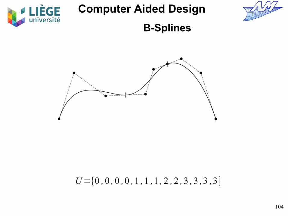
U={0 , 0 , 0 ,0 ,1 ,1 ,1 ,2 ,2 ,3 , 3 ,3 ,3}

105


B-Splines

U={0 , 0 , 0 ,0 ,1 ,1 ,1 ,2 ,2 ,2 ,3 ,3 ,3 ,3}

106


B-Splines

Bézier n°3 Bézier n°2 Bézier n°1 4 CP 4 CP 4 CPdegree 3 degree 3 degree 3

107


B-Splines

Differentiating B-splines For a B-Spline of typical nodal sequence:

We start from the definition of the derivatives of the basis functions:

Proof : Starting from N 1 and verify by induction that the relation is true for N d if it is true for N d-1 .

At the order k :

U={u0 ,⋯ , ud⏟d+ 1 times

,⋯ , um−d ,⋯, um⏟d+ 1 times

}

N id '=

duid−ui

N id−1

u−d

uid1−ui1

N i1d−1

u

∂k N i

d

∂ uk=

duid−ui

∂k−1 N i

d−1u

∂ uk−1−

duid1−ui1

∂k−1 N i1

d−1u

∂uk−1

108


B-Splines

N id '=

duid−ui

N id−1

u −d

uid1−ui1

N i1d−1

u

P 'u =∑

i=0

n

Pi N id 'u

P 'u =∑

i=0

n

duid−ui

N id−1

u −d

uid1−ui1

N i1d−1

u Pi

P 'u=d ∑

i=−1

n−1

N i1d−1

uPi1

uid1−ui1

−d∑i=0

n

N i1d−1

uP i

uid1−ui1

Change of index

109


B-Splines

P 'u=d ∑

i=−1

n−1

N i1d−1

uP i1

uid1−ui1

−d∑i=0

n

N i1d−1

uP i

uid1−ui1

P 'u=d∑

i=0

n−1

N i1d−1

u Pi1−P i

uid1−ui1

d P0 N 0d−1

u

ud−u0

−Pn1 N n1

d−1u

und1−un1

Empty Interval

0

P '(u)=∑

i=0

n−1

N i+1d−1

(u)Q i with Q i=dP i+1−P i

ui+d+1−ui+1

110


B-Splines

the nodal sequence used here remains :

We set

We've got a new B-Spline !

U={u0 ,⋯ , ud⏟d +1 times

,⋯, um−d ,⋯, um⏟d+1 times

}

P '(u)=∑

i=0

n−1

N i+ 1d−1

(u)Qi with Q i=dPi+ 1−P i

ui+ d + 1−ui+ 1

U '={u0

' ,⋯ , ud−1'

⏟d times

,⋯, um−d' ,⋯, um−2

'

⏟d times

} with ui'=ui+1

P '(u)=∑

i=0

n−1

N id−1

(u)Q i with N id−1 defined on U '

111


B-Splines

The 1st hodograph of a B-Spline of degree d is a B-Spline of degree d-1.

By successive derivation, the same holds for the kth hodograph.

U={0 ,0 , 0 , 2 , 4 , 6 ,6 ,6}

P0

P1 P2

P3

U '={0 ,0 ,2 , 4 , 6 ,6}

degree 2

degree 1

Q0

Q1

Q2

Q3

P4

P u P 'u

Q i=dPi+1−P i

ui+3−ui+2

=P i+1−P i

112


B-Splines

Derivative of order k

P(k )(u)=∑

i=0

n−k

N id−k

(u)P i(k ) with P i

(k )={

Pi k=0

(d−k+ 1)(Pi+ 1(k−1)

−P i(k−1)

)

ui+ d+ 1−ui+ k

k> 0

U (k )={u0

(k ) ,⋯ , ud−k(k )

⏟d+ 1−k times

,⋯ , um−d−k+ 1(k ) ,⋯, um−2k

(k )

⏟d+ 1−k times

} with ui(k )=ui+ k

113


B-Splines

Knot removal Inverse of Boehm's algorithm Given here without demonstration – the manipulations

leading to this result are simple but tedious Cf JC Leon «Modelisation de courbes et surfaces pour la CFAO» ,

hermès (1991) - pp352-353

114


B-Splines

Knot removal At each node, the continuity is at least Cd-s where s is

the multiplicity of the node. A curve of degree 3 has a continuity C2 if the nodes are simple

(multiplicity 1).

In the case where the effective continuity Cr of the curve at a given node is higher than Cd-s , one can decrease the multiplicity of the node by t=d-s-r.

If it is not the case, one cannot remove the node without changing the shape of the curve.

Before effectively removing a node, one must check the continuity of the curve on both sides of the node. The next algorithm allows to decide this while computing the new control points.

115


B-Splines

We try to delete the knot of multiplicity s.

u=ur≠ur1

i = r - d ; j = r - swhile ( j – i > 0 )

compute

compute

i = i + 1 ; j = j – 1end while

i=u−ui

uid1−ui

j=u−u j

u jd1−u j

P i1=

P i0−1−iP i−1

1

i

P j1=

P j0− j P j1

1

1− j

These two terms are known for the first iterationthey are respectively and .Pr−s1

0Pr−d−10

116


B-Splines

Testing the possibility to remove the knot

if (i=j) computecompute the distance between P and the control point P

i

otherwise compute the distance between

If the distance is lower than a tolerance T, replace the control points P

k by the new control points P

k1 and update the nodal sequence as

well.

P=i P i−11

1−i Pi11

P i−11 and P j+ 1

1

117


B-Splines

Practical example:deletion of

U={0 ,0 , 0 ,0 ,1 ,1 ,2 , 2 , 2 , 2}

P0

P1

P2P3

P4

P5

u=u5

118


B-Splines

Deletion of (r=5 , d=3 , s=2)

U={0 ,0 , 0 ,0 ,1 ,1 ,2 , 2 , 2 , 2}

P0

P1

P2P3

P4

P5

u=u5

i=r-d=2 j=r-s=3 2=u−u2

u6−u2

=1 /2 3=u−u3

u7−u3

=1 /2

P21=

P20−(1−α2)P1

1

α2=2 P2

0−P1

1 P31=

P30−α3 P4

1

1−α3

=2 P30−P4

1

P31P2

1

119


B-Splines

New control polygon

U={0 ,0 , 0 ,0 ,1 , 2 , 2 ,2 ,2}

P0

P1

P3

P4

P2

120


B-Splines

Now, deletion of (r=4 , d=3 , s=1)

U={0 , 0 ,0 ,0 ,1 ,2 ,2 , 2 ,2}

P0

P1

u=u4

i=r-d=1 j=r-s=3 1=u−u1

u5−u1

=1/2 3=u−u3

u7−u3

=1 /2

P11=

P10−1−1P0

1

1

=2 P10−P0

1 P31=

P30−3 P4

1

1−3

=2 P30−P4

1

P3

P4

P2P11

P31

121


B-Splines

Verification

U={0 , 0 ,0 ,0 ,1 ,2 ,2 , 2 ,2}

P0

P1

i=r-d=1 j=r-s=3

P3

P4

P2P11

P31

α2=u−u2

u6−u2

=1/2 P=α2 P11+(1−α2)P3

1=

P11+P3

1

2

P

OK !

122


B-Splines

Final control polygon U={0 , 0 , 0 ,0 , 2 , 2 ,2 ,2}

P0

P3

P1

P2

123


B-Splines

Restriction of the useful interval of a curve

Starting with a curve

defined on the nodal sequence:

We want to limit this curve at and Build the new control points Determine the new nodal sequence

P u=∑i=0

n

N iduPi

U={u0 ,⋯ , ud⏟d+ 1 times


}

u0* ul

*

P0

P1 P2

P3P4

P0*

P1*

P2*

P3*

P*u =∑

i=0

k

N idu Pi

*

U *={u0

* ,⋯ , ud*

⏟d+ 1 times

,⋯ , ul−d* ,⋯, u l

*

⏟d+ 1 times

}

u0* u l

*

P i*

U *

124


B-Splines

Use of the Boehm's algorithm Knot insertion up to a multiplicity equal to d.u=u0

*

P0

P1 P2

P3P4

u0*

U={0 , 0 , 0 , 2 , 4 , 6 ,6 ,6}

u0*=1

P0'

u0*

U '={0 ,0 , 0 , 1 ,1 ,2 ,4 ,6 ,6 ,6}

P1'

P2'

P3'

P4'

P5'

P6'

125


B-Splines

Use of the Boehm's algorithm Knot insertion at until multplicity is equal to d. Knot insertion at until multiplicity iq equal to d.

The sequence of these operations is not important.

u=u0*

u=ul*

P0'

u0*

U '={0 ,0 , 0 , 1 ,1 ,2 ,4 ,6 ,6 ,6}

P1'

P2'

P3'

P4'

P5'

P6'

U ''={0 , 0 ,0 ,1 , 1 ,2 , 3.5 , 3.5 , 4 ,6 ,6 ,6}

u l*

P0"

u0*

P1"

P2"

P3"

P4"

P7"

P8"

ul*=3.5

u l* P5

"

P6"

126


B-Splines

Use of the Boehm's algorithm Knot insertion in until multplicity is equal to d. Knot insertion in until multiplicity is equal to d.

The order of these operations is not important. Extraction of interesting part of the curve and addition of knots at the

start and end of the nodal sequence so as to have a multiplicity equal to d+1 at both extremities

u=u0*

u=ul*

U ''={0 , 0 ,0 ,1 , 1 ,2 , 3.5 ,3.5 , 4 ,6 ,6 ,6}

u l*

P0"

u0*

P1"

P2"

P3"

P4"

P7"

P8"

P5"

P6"

U *={1 ,1 ,1 , 2 , 3.5 ,3.5 ,3.5}

P0*

P1*

P2*

P3*

127


B-Splines

U={0 , 0 ,0 ,0,1 , 2 ,3 ,3 ,3 , 3}

128


B-Splines

U={0 , 0 ,0 ,0 ,0.2 ,0.2 ,0.2 ,1 , 2 ,3 , 3 , 3 ,3}

129


B-Splines

U={0.2 ,0.2 ,0.2 ,0.2 ,1 , 2 ,3 , 3 , 3 ,3}

130


B-Splines

U={0.2 ,0.2 ,0.2 ,0.2 ,1 , 2 , 2.9 , 2.9 ,2.9 , 3 ,3 ,3 ,3}

131


B-Splines

U={0.2 ,0.2 ,0.2 ,0.2 ,1 , 2 ,2.9 ,2.9 , 2.9 , 2.9}

132


B-Splines

Increase of a curve's useful interval

We want to extend the curve toor to

P u=∑i=0

n

N iduPi U={u0 ,⋯ , ud⏟

d+ 1 times


}

P0

P1 P2

P3P4

u0*

u=u0*u0

u0

u=um*um

133


B-Splines

We cannot use the node insertion algorithm directly Instead, use of Cox-de Boor's algorithm

« backwards » to determine the new position of the control points

We move the node to . The new nodal sequence is :

P0

P1 P2

P3P4

u0*

u0

u0*u0

U *={u0

* ,⋯ , ud*

⏟d + 1 times

, ud+ 1 ,⋯, um−d ,⋯ , um⏟d+ 1 times⏟

unchanged

}

P i*

134


B-Splines

We calculate the point corresponding to u0 from

unknown positions of control points Sequence of points obtained with the Cox-de Boor algorithm :

Among these points : The points are known (they are the points P

i !)

Only the d+1 first control points are affected (the interval concerned by Cox-de Booris [u

i, u

i+1[, i=d ).

P j* k= u0−u j

*

u jd1−k*

−u j* P j

* k−1 u jd1−k

*−u0

u jd1−k*

−u j* P j−1

* k−1

P0=P 2* 2

P1=P2*1

P3=P3*P4=P 4

*

u0*

u0

P0*0=P0

*

P i*

Pd*d −i

P2=P 2*0

For k from 1 to d For j from i to i-d+k

for k from 1 to d for j from d to k

135


B-Splines

P j* k= u0−u j

*

u jd1−k*

−u j* P j

* k−1 u jd1−k

*−u0

u jd1−k*

−u j* P j−1

*k−1For k from 1 to d For j from d to k

Is transformed in :

P j−1* k−1

= u jd1−k*

−u j*

u jd1−k*

−u0P j

* k− u0−u j

*

u jd1−k*

−u j* u jd1−k

*−u j

*

u jd1−k*

−u0P j

* k−1

Initialise For j from d to 1 For k from j to 1

known

P j−1* k−1

= u jd1−k*

−u j*

u jd1−k*

−u0P j

* k u j

*−u0

u jd1−k*

−u0P j

* k−1

Pd* d−i

=Pi

136


B-Splines

P2* 2

P2*1 P2

*0

P3*P4

*

U *={−0.1 ,−0.1 ,−0.1 ,1 ,2 ,3 ,3 , 3}

P j−1* k−1

= u j3−k*

−u j*

u j3−k* P j

*k u j

*

u j3−k* P j

* k−1

U={0 , 0 , 0 ,1 ,2 ,3 , 3 ,3}d=2 u0=0

u0*=−0.1

For j from 2 to 1 For k from j to 1

P1*1= u3

*−u2

*

u3* P2

* 2 u2

*

u3* P2

*1

P1*1=1.1 P2

* 2−0.1 P2

*1

P1* 0= u4

*−u2

*

u4* P2

* 1 u2

*

u4* P2

* 0

P1* 0=1.05 P2

*1−0.05 P2

* 0

P1*0j=2 k=2

j=2 k=1

P1*1

137


B-Splines

P2* 2

P2*1 P2

*0

P3*P4

*

U *={−0.1 ,−0.1 ,−0.1 ,1 ,2 ,3 ,3 , 3}

P j−1* k−1

= u j3−k*

−u j*

u j3−k* P j

*k u j

*

u j3−k* P j

* k−1

U={0 , 0 , 0 ,1 ,2 ,3 , 3 ,3}d=2 u0=0

u0*=−0.1

For j from 2 to 1 For k from j to 1

P0*0=1.1 P1

*1−0.1 P1

*0

P1*0j=1 k=1

P0* 0= u3

*−u1

*

u3* P1

*1 u1

*

u3* P1

* 0

P1*1

P0*0

138


B-Splines

P2*0

P3*P4

*

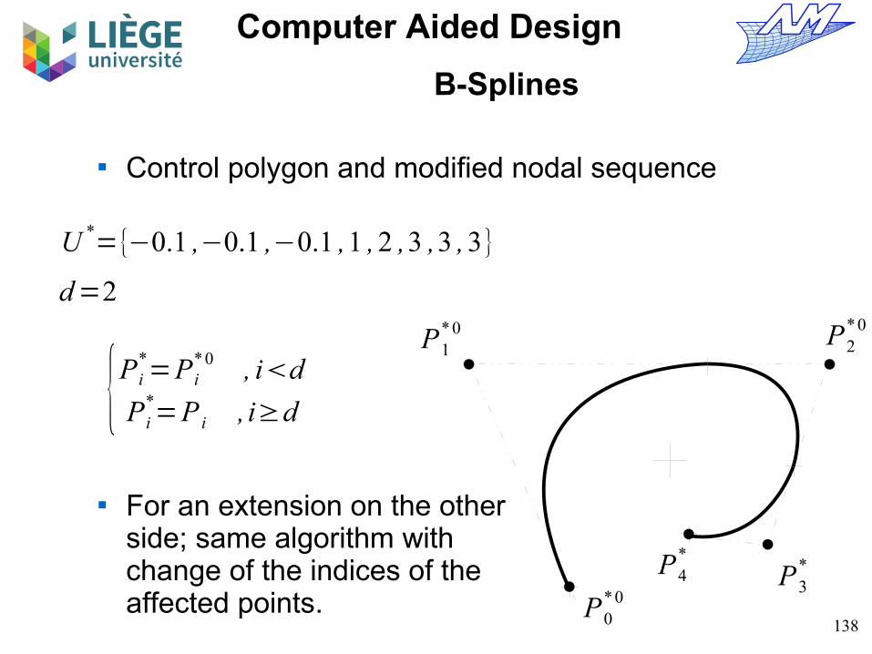
U *={−0.1 ,−0.1 ,−0.1 ,1 , 2 ,3 ,3 , 3}

d=2

P1*0

P0*0

{Pi*=Pi

*0 , id

Pi*=P i , i≥d

Control polygon and modified nodal sequence

For an extension on the otherside; same algorithm with change of the indices of the affected points.

139


B-Splines

U={0 , 0 , 0 ,0 ,1 , 2 , 3 , 3 ,3 ,3}

140


B-Splines

Increase for u=-0.1

U={−0.1 ,−0.1 ,−0.1 ,−0.1 ,1 , 2 ,3 ,3 ,3 ,3}

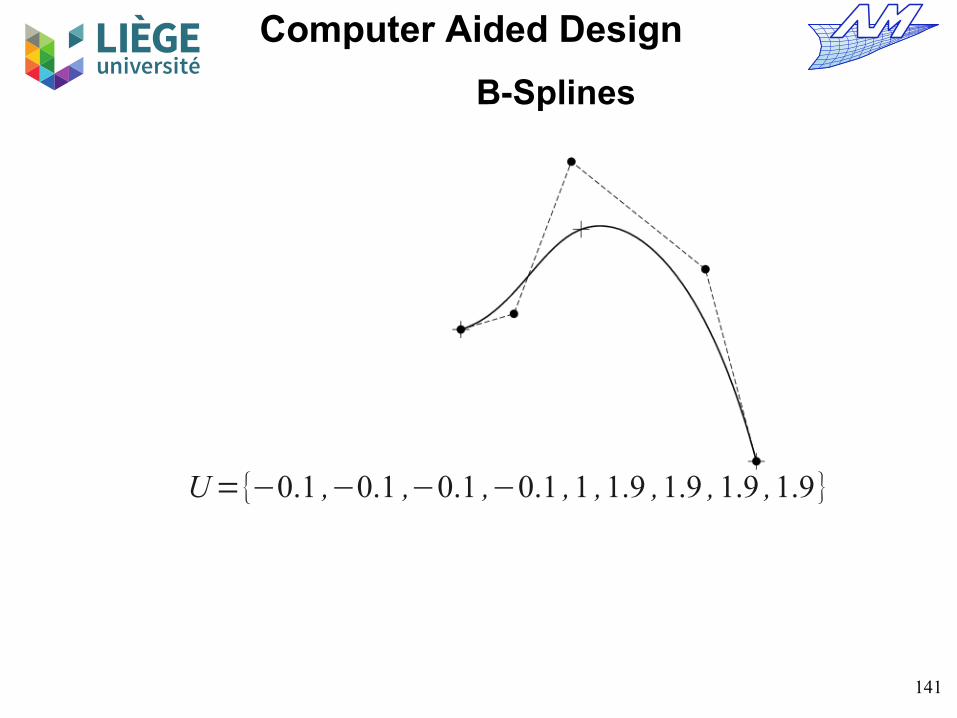
141


B-Splines

U={−0.1 ,−0.1 ,−0.1 ,−0.1 ,1 ,1.9 ,1.9 , 1.9 ,1.9}

142


B-Splines

Degree elevation A B-spline curve of degree d can be converted without

loss into a curve of degree d+1. Proof : shape functions of degree d+1 “contain” those of degree d.

The continuity of the curve of degree d at the nodes is given by the nodal sequence.

For a same multiplicity of a node, the curve of degree d+1 offers a higher continuity.

As a consequence, in the nodal sequence of the new curve, one must increment the multiplicity of each node.

143


B-Splines

Degree elevation algorithm Several algorithms exist :

Tiller et al (1983) Direct resolution of a linear system

Prautzch et al. (1991) Cf JC Leon, « Modélisation de curves et surfaces pour la CFAO »

Piegl et al. (1994) Competitive with Prautzch (specially for multiple elevations) Transform the curve in succession of Bézier curves by insertion of

nodes (multiplicity = d) Increase the degree of Bézier curves (ref. ad-hoc algorithm as seen

for Bézier curves) Removal of most of nodes that were introduced

144


B-Splines

Recursive subdivision As in the case of Bézier curves, one can increase the

number of CPs , this time using Boehm's knot insertion algorithm instead of De Casteljau's.

The control polygon converges to the curve as one inserts new knots ( each time in the middle of the widest knot interval)

The usual order of B-Spline curves is small (3 or 4, maybe 5), so savings in computational complexity with respect to a systematic evaluation with Cox-de Boor's algorithm are not so dramatic.

145


B-Splines

Some conclusions Flexibility Low order Continuity Periodic curves Conics ?

146


Rational curves« Non Uniform Rational B-Splines »

147


NURBS

Representation of conic sections Circles , ellipses, hyperbolas... A fair number of « industrial » geometries do have

conic sections in their definition Bézier curves, B-Splines and other polynomial

representations cannot exactly represent all conic sections

148


NURBS

Example : the circular arc Parametric form A

u is the angle

No polynomial representation (or as a series) Parametric form B

Problem : square root

{x u=cos uy u=sin u

, u∈[0,2]

{x u =1−uy u=u 1−u

, u∈[0,1]

u

u

149


NURBS

Parametric form C

Ratio of two polynomials of degree 2 x(u) and y(u) have a common denominator

u

{x (u)=

2u

1+u2

y (u)=1−u2

1+u2

, u∈[0,1]

150


NURBS

Thus, one can set the following :

P u=P w

uw u

Vectorial term

Weight function (scalar)

{x (u)⋅w (u)=2 u

y (u)⋅w (u)=1−u2

w (u)=1+u2

, u∈[0,1]

151


NURBS

Non rational curves

Rational curves

A weight wi is associated to every control point P

i ,

A scalar approximation w(u) is built on the same model as for regular B-Splines

P u=∑i

N idu P i

P (u)=∑

i

N id(u)P i w i

∑j

N jd(u)w j

=P w

(u)w (u)

=∑i

Rid(u)Pi

with Rid(u)=

N id(u)wi

∑j

N jd(u)w j

152


NURBS

Relation between conics and the central projection With respect to central projection; all conics are equivalent.

O

circle

ellipse

parabola

hyperbola

cone

153


NURBS

In particular, parabolas may be modelled with polynomials.

Any other conic section can be obtained by projecting a parabola onto an appropriately oriented plane.

O

circle

parabola

154


NURBS

Central projection and homogeneous coordinates Everything takes place in a 4-dimensional space We have a class of equivalence :

This equivalence class is a central projection of all the points located on a straight line passing by the origin onto the plane of equation w=1

How to get cartesian 3D coordinates from the homogeneous 4D coordinates :

Just divide all the components by the 4th component Discard the 4th component (it is equal to one)

[wx , wy , wz , w ]≡[ x , y , z ,1] ∀w>0

155


NURBS

Projection of a parabola to a circle

O

circle

parabola

Homogeneous coordinate “w”

Regular coordinates x, y (, z)

1

156


NURBS

In practice .. one works on the 4 homogeneous coordinates

In this space, we just know how to represent parabolas.

The equivalence class allows us to divide by the last component and bring us back to euclidean 3D space

We can therefore represent any conic section. How to determine the right control points ?

P w(u)=∑

i

N id(u)P i

w with Piw=(

x i⋅wi

y i⋅wi

zi⋅w i

w i

)

P iw

157


NURBS

Representation of 1/3rd of a circle with the help of B-splines (or Bézier) curves...

3 control points, nodal sequence [0,0,0,1,1,1] (a parabola) We must determine homogeneous coordinates of each control point

so that the central projection yields points exactly on the arc.

A BA' B'

C

w=1

Plane containing the parabola

BAC'

w=0

A=A'=[−r3 /2

r /201

] B=B '=[r 3 /2

r /201

] C '=[0

3 r /40

3/4]

O

P1w

P 2w

=B'

P 0w

=A'

w=3/2

C

Plane of thecircle

P0w=A'

P2w=B '

P1w=2C '−

A'B ' 2

=[0r0

1/2]

C'

w=3/4In the plane of the parabola

In the planeof the circle

C=[0r01]

158


NURBS

3 r

32

rw=

12

w=14

w=110

w=1

w=2

w=4

w=10

1/3 of a circle

U=[0 , 0 , 0 ,1 ,1 ,1]

159


NURBS

Complete circle in three pieces

A single B-spline NURBS Non uniform Rational

U=[0 ,0 ,0 ,1 ,1 ,2 ,2 ,3 ,3 ,3]

w=12

w=1

160


NURBS

Parametrization

U=[0 ,0 ,0 ,1 ,1 ,2 ,2 ,3 ,3 ,3]

161


NURBS

Generalization : Circular arc of angle α <= 2p/3 (actually, <p)

P0w

P1w

P2w

2r sin

2

r tan

2sin

2

r cos

2

w=cos

2

w=1 w=1P1

w=

x1 cos/2y1 cos/2z1 cos/2cos/2

P0w=

x0

y0

z0

1

P2w=

x2

y2

z2

1

162


NURBS

Can we represent a circle with only 2 pieces ?- yes if we allow control points with w=0

P1w=[

0r00]

P0w=P 4

w=[

−r001] P2

w=[

r001]

U=[0 ,0 ,0 ,1 ,1 ,2 ,2 , 2]

P3w=[

0−r00]

163


NURBS

Can we represent a circle as a single piece ?No (if we remain with degree 2)

Interval for the parameter necessary to cover the whole circle : The nodal sequence is therefore undefined

ℝ

164


NURBS

Can we represent a circle as a single piece ?Yes : if we accept to increase the degree (here 5)

P0w=P5

w=[

0−5 r

05

]P1

w=[

−4 r−r01

] P4w=[

4 r−r01]

P2w=[

−2 r3 r01

] P3w=[

2 r3 r01]

165


NURBS

Properties of the NURBS basis functions

P (u)=∑

i

N id(u)P i w i

∑j

N jd(u)w j

=P w

(u)w (u)

=∑i

Rid(u)Pi

with Rid(u)=

N id(u)w i

∑j

N jd(u)w j

166


NURBS

Partition of the unity: with

In fact, there is always partition of unity with this definition. The original shape functions (N) must however be all linearly independent, and not all equal to zero at any point...

Ridu=

N iduw i

∑j

N jduw j

∑i

Ridu=1

∑i

N id(u)wi

∑j

N jd(u)w j

≡1 iff ∑j

N jd(u)w j≠0

167


NURBS

Properties of NURBS basis functions Non-negativity Partition of the unity If the nodal sequence is not periodic (d+1 repetitions)

one have reaches exactly one maximum on the definition

interval (for d>0) Compact support : Every derivative exist inside a nodal interval, at one

node, SFs are differentiable at least d-k times (k is the multiplicity of a node)

If wi=cst, we have classical non rational curves.

Ridu ≥0 Ri

du =

N iduwi

∑j

N jduw j∑

i

Ridu=1

R0d0=Rn

d1=1

Ridu

Rid(u)=0 for u∉[ ui , ui+ d + 1[

168


NURBS

These properties have the same consequences on the curve as in the classical B-Spline case

Beware : the wi must remain positive. They may vanish iff w(u)

remain always strictly positive.

Affine invariance Convex hull Local control of a given control point etc...


NURBS

Modification of the weight of a control point Does not change the 3D position of the control point

(only the distance to the perspective plane in the central projection)

Modify the « attraction » of the control point with respect to the curve

Means to modify the shape of the curve without moving control points

No changes in the geometric continuity of the curve Interesting at the junction of independent curves : the continuity of

tangents at the interface is not disturbed – even if the modification is not local (ex: for Bézier curves)


NURBS

Location of a given point when modifying a weight...

We modify the weight wi0 associated to the point P

i0

Set

The point is on the straight line joining NM

The straight line NM passes by Pi0 (limit case )

( Also also true for rational surfaces as seen later...)

N=P (u)|wi 0=1

M=P (u)|w i 0=0

P=P (u) , w i 0≥0

w i 0→∞

wi 0=1

wi 0→∞

wi 0=0

N

M


NURBS

Proof

P (u)=∑i≠i 0

N ip(u)P i w i+N i 0

p(u)P i 0 w i 0

∑k≠i 0

N kp(u)wk+N i 0

p(u)w i 0

P (u)=P+n P i 0 wi 0

w+n w i 0

N=P+n Pi 0

w+nM=

Pw

P=M w

N=M w+n P i 0

w+nP i 0=

N (w+n)−M wn

P (u)=P+n P i 0 wi 0

w+n w i 0

=M w+(N (w+n)−M w)w i 0

w+nw i 0

=

N(w+n)w i 0

w+n w i 0

+M(w−w w i 0)

w+n w i 0

=N f (w i 0)+M g (w i 0)

172


NURBS

Calculating NURBS derivatives Presence of the rational term : rules of derivation are

more complex. Set

So :

Au=w u ⋅P u

P u=Au w u

3 first components of the homogeneous coordinates

last component of the homogeneous coordinates

P '(u)=

w (u) A'(u)−w'

(u)A(u)

w (u)2 =w (u) A'

(u)−w '(u)w (u)P (u)

w (u)2

=A'u−w '

uP uw u

173


NURBS

Derivatives (general case at the order k)Au=w u ⋅P u

Ak u =∑

i=0

k

ki wi u ⋅Pk−i

u

=w u Pk u∑

i=1

k

ki wiu⋅Pk−i

u

P k u=

Ak u −∑

i=1

k

ki wiu ⋅Pk−i

u

w u

b-splines - uliege · 3 computer aided design b-splines isaac j. schoenberg (1946) carl de boor...

Documents