1

BA 513: Ph.D. Seminar on Choice Theory Professor Robert Nau Spring Semester 2007 Notes and readings for class #1 (updated December 17, 2007) At our first class meeting we will discuss the broad outlines of rational choice theory, touch on a few of the controversial issues that will be treated in more depth later in the course, and review the early history of utility theory, focusing in particular on the contributions of the marginalist revolution in economics that occurred in the 1870's, at which time utility functions were first used to model interactions among groups of agents in competitive markets. This will provide some background on the concept of “ordinal” utility, prior to our discussions of “cardinal” expected utility in the next few class meetings, as well as provide an introduction to the prototypical concept of equilibrium behavior. The readings for this class meeting are divided into primary and supplementary categories, as follows. 1. Primary readings:

a. “Rationality of self and others in an economic system” by Kenneth Arrow, 1986 b. “The development of utility theory” by George Stigler, 1950 c. Excerpt on the “The Marginalist Revolution of the 1870's” by Philip Mirowski, 1988

2. Supplementary readings:

a. Excerpts from chapters 5 & 6 of the microeconomics text by David Kreps, 1990 1.1 Introduction Rational choice theory is social physics: a search for universal mathematical laws to explain social and economic phenomena in terms of the behavior of their fundamental particles, namely human decision makers. In rational choice models, individuals strive to satisfy their preferences for the consequences of their actions given their beliefs about events, which are represented by utility functions and probability distributions, and interactions among individuals are governed by equilibrium conditions. This paradigm includes most standard models of mathematical economics, finance theory, and statistical decision theory, as well as other areas of business research such as marketing (e.g., distribution channels), operations management (e.g., supply chains), and accounting (e.g., auditor-auditee relationships). It also includes rational-actor models that have become prominent—and controversial—in other fields such as political science, sociology, law, and philosophy. In its modern form, rational choice theory dates back 50 or 60 years to a trio of seminal publications: von Neumann and Morgenstern’s Theory of Games and Economic Behavior (1944/1947), Kenneth Arrow’s Social Choice and Individual Values (1951), and Savage’s Foundations of Statistics (1954). These publications were part of a general ferment of cross-disciplinary operational research during the early post-war era, and they laid the foundation for a dramatic escalation in the use of mathematical methods in the social sciences—especially axiomatic methods, concepts of measurable utility and

2

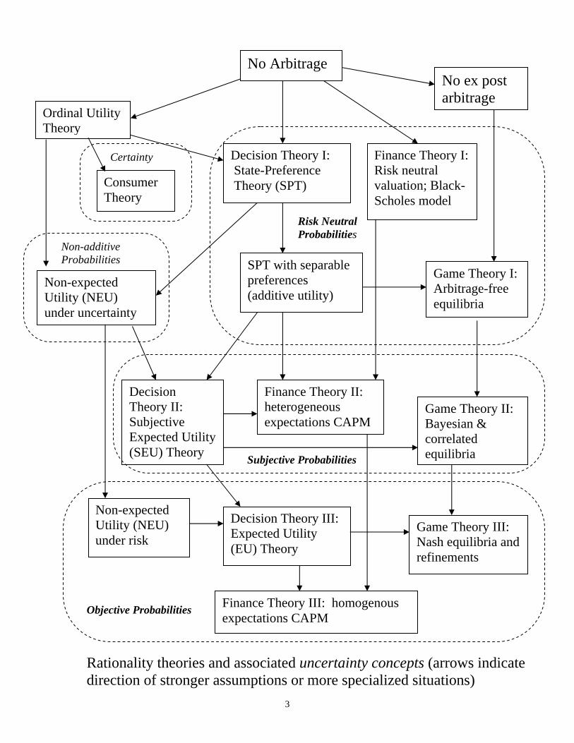
personal probability, and tools of general equilibrium theory and game theory. But rational choice theory has roots that go back much farther—to the first formal use of equilibrium models by marginalist economists in the late 1800’s, to the proposal of the concept of expected-utility-maximization by Bernoulli in the early 1700’s, to the emergence of the theory of probability in the 1500’s and 1600’s, and even back to the development of the axiomatic method by Euclid. In this first class, we will (i) discuss some of the broad issues in rational choice theory that are touched on in the primary readings and (ii) discuss the history of utility theory with particular emphasis on the fundamentals of consumer theory that were developed during the marginalist revolution, namely the use of ordinal utility functions to represent preferences among commodities, the principle of equi-marginal-utility, the Edgeworth box, the concepts of Walrasian general equilibrium and Pareto optimality, and their connections with the principle of no-arbitrage. Much of this material may be familiar to you if you have already had a course in microeconomics, but the following pages provide a quick review of the main ideas. I hope no one is offended by the economics-101 tone of my discussion of consumer theory. When I previously taught the course, I found that this material was not familiar to everyone, and in any case I want to add some of my own spin to old and familiar results. Before plunging in, here is a road map of some of the territory we will explore in the early part of this course. We will study various models of individual rationality (single-agent behavior), strategic rationality (small-group behavior), and competitive rationality (large-group behavior). Models of individual rationality include ordinal utility (for choice under conditions of “certainty”), expected utility (for choice under conditions of “risk,” where probabilities for events are objectively determined), subjective expected utility and state-preference theory (for choice under conditions of “uncertainty,” where probabilities for events are subjectively determined—or perhaps undetermined), and several kinds of non-expected utility theory (in which total utility is not representable as a sum of utilities associated with disjoint events). Models of strategic rationality include a wide spectrum of different equilibrium concepts of game theory. Models of competitive rationality include the general equilibrium model and particular forms of it that are used in asset pricing theory in finance. The diagram on the following page shows a rough taxonomy of these theories, arranged according to the strength of their assumptions and the representations of uncertainty that they incorporate (objective probabilities, subjective probabilities, risk neutral probabilities, non-additive probabilities, etc.). This may look like a lot of ground to cover—and it is—but I will try to focus on the key underlying assumptions (rather than mathematical intricacies) and on the deep connections among the theories. At the top of the diagram is the principle of no-arbitrage, which (I will argue) is the most fundamental principle of economic rationality and which will turn out to be the common denominator of many of the other theories. By no-arbitrage, I mean the requirement that an individual should be rational in the sense of not offering to accept bets or commodity trades that could result in a sure loss, i.e., she should not offer to throw money away. A slightly stronger requirement, which will turn out to be more useful in the context of game theory, is that of no ex post arbitrage, under which the individual should not offer to accept bets or trades that would have resulted in a loss, given the way events turned out, without having offered the possibility of a gain had events turned out otherwise. Later in the course, after we have covered some of the basic theory, we will discuss applications of rational choice theory as well as controversies and alternative paradigms.

3

Ordinal Utility Theory

Consumer Theory

Finance Theory I: Risk neutral valuation; Black-Scholes model

SPT with separable preferences (additive utility)

Decision Theory II: Subjective Expected Utility (SEU) Theory

Decision Theory III: Expected Utility (EU) Theory

Game Theory I: Arbitrage-free equilibria

Game Theory II: Bayesian & correlated equilibria

Game Theory III: Nash equilibria and refinements

Non-expected Utility (NEU) under uncertainty

Non-expected Utility (NEU) under risk

Certainty

Risk Neutral Probabilities

Non-additive Probabilities

Subjective Probabilities

Objective Probabilities Finance Theory III: homogenous expectations CAPM

Rationality theories and associated uncertainty concepts (arrows indicate direction of stronger assumptions or more specialized situations)

Finance Theory II: heterogeneous expectations CAPM

Decision Theory I: State-Preference Theory (SPT)

No ex post arbitrage

No Arbitrage

4

1.2 Mathematical foundations: three pillars…. or one?

At bottom, rational choice theory rests upon a set of primitive axioms and fundamental theorems which imply that rational behavior has convenient numerical representations within which familiar tools of applied mathematics (calculus, matrix algebra, convex analysis, etc.) can be used to describe and predict what rational actors should do in various institutional settings. These mathematical foundations are typically divided into three main pillars: (i) axioms and theorems that govern the preferences of rational individuals and which allow those preferences to be represented by numbers such as probabilities and utilities; (ii) the fixed point theorem that is used to prove the existence of equilibria in games and markets where two or more individuals interact, and (iii) the separating hyperplane theorem that is used in many different contexts to obtain results such as the two theorems of welfare economics, the laws of subjective probability, and formulas for asset pricing in financial markets. Before we get started, you should try to fix these three key concepts in your head:

• The preference axioms include requirements such as completeness (given any two alternatives, at least one must be weakly preferred to the other—a rational person is never undecided), transitivity (a sequence of pairwise preferences, at least one of which is strict, should not form a cycle), reflexivity (an alternative is weakly preferred to itself), continuity (if a sequence of alternatives{xn} converges to x, and another sequence{yn} converges to y, and xn is weakly preferred to yn for all n, then x must also be weakly preferred to y), and various kinds of independence conditions (the direction of preference between two alternatives should not depend on features they have in common). Such axioms imply the existence of appropriate numerical scales on which beliefs and values can be measured.

• The fixed point theorem states that every continuous mapping (or more generally, an upper hemicontinuous correspondence) of a convex compact set into itself has at least one fixed point. For example, if you have pan of pizza dough, you can’t push it around smoothly and keep it all in the pan without leaving at least one morsel back in the same place after you are done—try it. (Note: convexity means that a line segment between any two points in the set is wholly contained in the set, ruling out objects with holes in them such as circles or cylinders, whose points could be rotated around the center without leaving any point fixed. Compactness means that the set is both closed and bounded, which rules out lines or planes extending to infinity that could be slid in one direction without leaving any point fixed, as well as open sets in which all points could be moved partway to an edge without leaving any point fixed.) In models of games and competitive economies, the relevant set is a set of strategies or resource allocations for two or more individuals or firms, the mapping is a “best-reply correspondence” in which each agent responds optimally to the status quo, and the fixed point is an equilibrium such that once it is reached, no one will have an incentive to deviate to some other point.

• The separating hyperplane theorem states that any two disjoint convex sets, at least one of which is an open set, can be separated by a hyperplane (a generalized plane in n dimensions). For example, in three dimensional space, convex sets are geometrical objects such as spheres, ellipsoids, polyhedrons, cones, and half-spaces—but not donuts or bananas. The theorem states that if you have two such objects, and they do not intersect, then you can pass a flat sheet of paper between them. This may seem geometrically obvious, but it turns out to have rather profound implications. One of the themes of this course will be to show that the separating hyperplane theorem is the most important of the three pillars and that by itself it delivers all of the most fundamental theorems of rational choice when it is used in the context of no-arbitrage arguments.

5

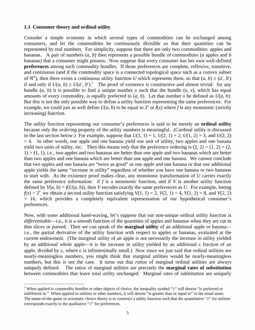
1.3 Consumer theory and ordinal utility

Consider a simple economy in which several types of commodities can be exchanged among consumers, and let the commodities be continuously divisible so that their quantities can be represented by real numbers. For simplicity, suppose that there are only two commodities: apples and bananas. A pair of numbers (a, b) then represents a possible bundle of commodities (a apples and b bananas) that a consumer might possess. Now suppose that every consumer has her own well-defined preferences among such commodity bundles. If those preferences are complete, reflexive, transitive, and continuous (and if the commodity space is a connected topological space such as a convex subset of ℜn), then there exists a continuous utility function U which represents them, so that (a, b) ≥ (a′, b′) if and only if U(a, b) ≥ U(a′, b′).1 The proof of existence is constructive and almost trivial: for any bundle (a, b) it is possible to find a unique number x such that the bundle (x, x), which has equal amounts of every commodity, is equally preferred to (a, b). Let that number x be defined as U(a, b). But this is not the only possible way to define a utility function representing the same preferences. For example, we could just as well define U(a, b) to be equal to 2x or f(x) where f is any monotonic (strictly increasing) function.

The utility function representing our consumer’s preferences is said to be merely an ordinal utility because only the ordering property of the utility numbers is meaningful. (Cardinal utility is discussed in the last section below.) For example, suppose that U(1, 1) = 1, U(2, 1) = 2, U(1, 2) = 3, and U(2, 2) = 4. In other words, one apple and one banana yield one unit of utility, two apples and one banana yield two units of utility, etc. Then this means only that the preference ordering is (2, 2) > (1, 2) > (2, 1) > (1, 1), i.e., two apples and two bananas are better than one apple and two bananas which are better than two apples and one banana which are better than one apple and one banana. We cannot conclude that two apples and one banana are “twice as good” as one apple and one banana or that one additional apple yields the same “increase in utility” regardless of whether you have one banana or two bananas to start with. As the existence proof makes clear, any monotonic transformation of U carries exactly the same preference information: if f is a monotonic function, and if V is another utility function defined by V(a, b) = f(U(a, b)), then V encodes exactly the same preferences as U. For example, letting f(x) = 2x

, we obtain a second utility function satisfying V(1, 1) = 2, V(2, 1) = 4, V(1, 2) = 8, and V(2, 2) = 16, which provides a completely equivalent representation of our hypothetical consumer’s preferences.

Now, with some additional hand-waving, let’s suppose that our non-unique ordinal utility function is differentiable—i.e., it is a smooth function of the quantities of apples and bananas when they are cut in thin slices or pureed. Then we can speak of the marginal utility of an additional apple or banana—i.e., the partial derivative of the utility function with respect to apples or bananas, evaluated at the current endowment. (The marginal utility of an apple is not necessarily the increase in utility yielded by an additional whole apple—it is the increase in utility yielded by an additional ε fraction of an apple, divided by ε, where ε is infinitesimally small.) Now since we just said that ordinal utilities are nearly-meaningless numbers, you might think that marginal utilities would be nearly-meaningless numbers, but this is not the case. It turns out that ratios of marginal ordinal utilities are always uniquely defined. The ratios of marginal utilities are precisely the marginal rates of substitution between commodities that leave total utility unchanged. Marginal rates of substitution are uniquely

1 When applied to commodity bundles or other objects of choice, the inequality symbol “≥” will denote “is preferred or indifferent to.” When applied to utilities or other numbers, it will denote “is greater than or equal to” in the usual sense. The name-of-the-game in axiomatic choice theory is to construct a utility function such that the quantitative “≥” for utilities corresponds exactly to the qualitative “≥” for preferences.

6

determined by preferences and as such they are observable, hence any two utility functions that represent the same preferences must yield the same ratio of marginal utilities between any two commodities. Thus, for example, it might be the case that the ratio of the marginal utilities of apples to bananas is equal to 1/2 when the consumer already has one apple and one banana, meaning that the consumer would indifferently trade an ε fraction of an additional banana for a 2ε fraction of an additional apple. Then the same ratio must be obtained for any other utility function that is a monotonic transformation of the original one. This follows from the chain rule calculus: if V(a, b) = f(U(a, b)) as above, then

( , ) / ( ( , ))( ( , ) / ) ( , ) /( , ) / ( ( , ))( ( , ) / ) ( , ) /

V a b a f U a b U a b a U a b aV a b b f U a b U a b b U a b b

′∂ ∂ ∂ ∂ ∂ ∂= =

′∂ ∂ ∂ ∂ ∂ ∂

where f′ (x) denotes the derivative of f at x, so the ratio of the marginal utility of an apple to that of a banana is the same under either U or V. Geometrically, what an ordinal utility function does is to determine the shape of indifference curves in the space of possible commodity bundles. An indifference curve is a set of points representing endowments that all yield the same numerical utility—i.e, that are equally preferred. For example, the consumer’s indifference curves might look like this in apple-banana space:

Here, points x and y are on the same indifference curve, meaning that they yield exactly the same utility—i.e., the consumer is precisely indifferent between them—whereas point z lies on a “higher” indifference curve, so it would be preferred to either x or y. Furthermore, the slope of a tangent line to an indifference curve (such as the dotted line through point y) is precisely the marginal rate of substitution between commodities at that point.

You can think of the preceding picture as a contour map of a three-dimensional utility surface on which the consumer would like to climb higher if at all possible. Thus, if the consumer started at point x on the map, she would be indifferent to walking around to point y, which is at the same elevation, but she would really prefer to climb higher up to point z. When thinking of the picture in this fashion, it is important to keep in mind that while the shapes of the indifference curves are uniquely determined by preferences, the relative heights of the utility surface above different indifference curves are completely arbitrary. Another utility function that represented the same preferences would have to

Apples

↑ Bananas

x

y

z

7

yield the same indifference curves, whose tangent lines would have exactly the same slopes at all points, but the corresponding utility surface might otherwise look very different. For example, under one ordinal utility function U, the three curves shown above might be equally spaced in utility units (i.e., in the third dimension), while under an equivalent utility function V, the jump in utility units from the first to the second curve might be 100 times as great as the jump from the second curve to the third curve. It is precisely because of this arbitrariness of an ordinal utility scale that economists in the early 1900’s gradually began to emphasize indifference-curve analysis and to scorn the concept of utility functions.

Armed with our knowledge that ratios of marginal utilities equal marginal rates of substitution, we can make our first not-quite-trivial observation about how such a rational consumer will behave in an economy. Suppose the consumer is initially endowed with some numbers of apples and bananas and is then placed in a market where apples and bananas can be bought and sold at fixed prices. For simplicity, assume that for each fruit the buying and selling prices are the same—i.e., there is no “friction.” What purchases or sales should the consumer make? The answer is that she should make purchases and sales to move to a new endowment at which the ratio of marginal utilities for apples and bananas equals the corresponding ratio of their prices. If this were not the case, then she could increase her total utility either by cashing in some apples to buy bananas or by cashing in some bananas to buy apples. A few additional assumptions are usually imposed at this point (if not earlier), namely that the consumer should have diminishing marginal utility for every commodity and she should never be entirely satiated with it. With these assumptions, there is usually a unique solution to the purchasing problem faced by a single consumer in a monetary economy.

The assumption of diminishing marginal utility was originally proposed by Bernoulli to help explain choices under risk—e.g., optimal gambling and insurance choices—and it was later resurrected by the marginalist economists to explain consumer choice under certainty. This assumption means that if we fix the holdings of all commodities except one, then the marginal utility of that commodity should decrease as the endowment of it increases. Meanwhile, non-satiation means that the marginal utility of every commodity always remains positive—i.e., it approaches zero only asymptotically, so that more is always better no matter how much you already have. Decreasing marginal utility is actually not a strong enough condition for the consumer’s purchasing problem to always have a unique solution unless the utility function is also additively separable—i.e., of the form U(a,b) = u1(a) + u2(b)—so nowadays a stronger assumption of strictly convex preferences is usually made, which means that if x ≥ z and y ≥ z, then αx+(1-α)y > z for any number α strictly between 0 and 1, where the vectors x, y, and z denote general multidimensional commodity bundles. In other words, if x and y are both weakly preferred to z, then everything in between x and y is strictly preferred to z. In particular, if x and y are equally preferred, then αx+(1-α)y is strictly preferred to either of them, i.e., the consumer would prefer to have a weighted average of x and y rather than either extreme. This property captures the intuition of diminishing marginal utility, namely that half an apple has more than half as much utility as a whole apple, but it does so by referring to observable preferences rather than unobservable utility. If preferences are strictly convex, then any utility function that represents those preferences is necessarily strictly quasi-concave, which means that its level sets are strictly convex sets, i.e., the set of all y such that U(y) ≥ U(x) is a strictly convex set. The strict convexity of the level sets ensures that the consumer’s purchasing problem in the presence of fixed prices has a unique solution. Another way to think of the consumer’s problem is in terms of optimization under a budget constraint. If the agent is given some initial endowment of commodities and is then placed in market where prices are already fixed, she can first sell her entire endowment to obtain a cash budget and then, subject to that budget constraint, she can buy a commodity bundle that maximizes her utility. In two dimensions,

8

the commodity bundles that she is able to purchase lie along the so-called budget line: the line whose slope is equal to the ratio of prices and which passes through her initial endowment point. For example, in the graph below, suppose the agent starts out with endowment x and that the dashed line represents the corresponding budget line—i.e., all the other endowments that cost the same as her initial endowment under the given prices. Then the optimal endowment for her to purchase is the point on the budget line that is touched by the indifference curve with the highest possible utility, to which the budget line is necessarily tangent. The optimal final endowment in this case is point y. Now suppose that two consumers, with different preferences and different initial endowments of apples and bananas, are placed in the same market. Then of course we should expect them both to optimize. If it is a frictionless market in which prices for apples and bananas are already fixed, then the agents can solve their optimization problems independently by transacting with other buyers and sellers. Their ratios of marginal utilities between apples and bananas will thereby end up the same as the ratio of prices, and hence they must end up having the same ratios of marginal utilities as each other. But suppose they are the only two agents in the economy and money does not exist, so that they can only trade apples and bananas with each other. Then their optimization problems are inextricably linked, and we need a more general definition of an optimal solution. From the viewpoint of an omniscient social planner, we might be tempted to solve a grand optimization problem that would maximize the total utility of both agents—the “greatest good of the greatest number” in Bentham’s terms. But we can’t do this because there is no such thing as total utility. The ordinal utilities of the two agents are arbitrary, incomparable numbers that cannot be meaningfully added or averaged together. But there is a weaker standard of joint optimization that can be used, namely the standard of Pareto optimality (also known as Pareto efficiency). A Pareto optimal allocation of commodities is an allocation that cannot be redistributed so as to make one agent better off without making the other worse off, each according to her own preferences. Note that this does not require direct numerical comparison of the utilities of one agent against those of another: we need only look at the signs (directions) of possible joint changes in utility, not their magnitudes. Given the opportunity to trade with each other, we should expect the agents to end up at a Pareto optimal point, because otherwise at least one agent could be made better off at no cost to anyone else. (In fact, if commodities and utility functions are continuous, it is usually possible to increase the utility of all agents if they are not already at a Pareto optimal point.) Significantly, this still requires that the agents should adjust their holdings so as to equalize the respective ratios of their marginal utilities for apples and bananas, because these are also their marginal rates of substitution, and if they did not have the same marginal rates of substitution, then an exchange of small bits of apple for small bits of banana

Apples

↑ Bananas

x (initial)

y (optimal)

Budget line

9

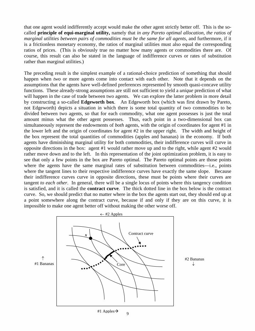
that one agent would indifferently accept would make the other agent strictly better off. This is the so-called principle of equi-marginal utility, namely that in any Pareto optimal allocation, the ratios of marginal utilities between pairs of commodities must be the same for all agents, and furthermore, if it is a frictionless monetary economy, the ratios of marginal utilities must also equal the corresponding ratios of prices. (This is obviously true no matter how many agents or commodities there are. Of course, this result can also be stated in the language of indifference curves or rates of substitution rather than marginal utilities.) The preceding result is the simplest example of a rational-choice prediction of something that should happen when two or more agents come into contact with each other. Note that it depends on the assumptions that the agents have well-defined preferences represented by smooth quasi-concave utility functions. These already-strong assumptions are still not sufficient to yield a unique prediction of what will happen in the case of trade between two agents. We can explore the latter problem in more detail by constructing a so-called Edgeworth box. An Edgeworth box (which was first drawn by Pareto, not Edgeworth) depicts a situation in which there is some total quantity of two commodities to be divided between two agents, so that for each commodity, what one agent possesses is just the total amount minus what the other agent possesses. Thus, each point in a two-dimensional box can simultaneously represent the endowments of both agents, with the origin of coordinates for agent #1 in the lower left and the origin of coordinates for agent #2 in the upper right. The width and height of the box represent the total quantities of commodities (apples and bananas) in the economy. If both agents have diminishing marginal utility for both commodities, their indifference curves will curve in opposite directions in the box: agent #1 would rather move up and to the right, while agent #2 would rather move down and to the left. In this representation of the joint optimization problem, it is easy to see that only a few points in the box are Pareto optimal. The Pareto optimal points are those points where the agents have the same marginal rates of substitution between commodities—i.e., points where the tangent lines to their respective indifference curves have exactly the same slope. Because their indifference curves curve in opposite directions, these must be points where their curves are tangent to each other. In general, there will be a single locus of points where this tangency condition is satisfied, and it is called the contract curve. The thick dotted line in the box below is the contract curve. So, we should predict that no matter where in the box the agents start out, they should end up at a point somewhere along the contract curve, because if and only if they are on this curve, it is impossible to make one agent better off without making the other worse off.

↑ #1 Bananas

#2 Bananas ↓

#1 Apples

← #2 Apples

x Contract curve

Core

10

Now let’s probe a little deeper. Suppose the agents start out at a given point in the Edgeworth box—say point x in the picture above. At what Pareto optimal point should they end up after they have had the opportunity to trade? All we can say is that they should end up somewhere on the segment of the contract curve that is at least as good as x for both agents—i.e., a point that lies above their respective indifference curves passing through x. Such a point is said to be Pareto superior to x. The portion of the contract curve that is Pareto superior to x is the heavy solid segment in the graph, and it is nowadays known as the core of the “market game” played by two agents who engage in trade starting from position x. (The basic concept of the core of a market game is due to Edgeworth, and it anticipates much later developments in the theory of cooperative games. More generally, the core of a game is the set of allocations that are stable against defections by coalitions.) We should expect the agents to end up somewhere in the core, but unless and until we pile on further assumptions, we cannot say exactly where in it they should end up. Thus, preferences alone do not suffice to determine the outcome of trade between agents. The outcome may depend as well on other psychological factors (e.g., on which of the two agents is more patient, more stubborn, more savvy, etc.), or on market mechanisms that somehow restrict the trades they are able to make, or on environmental contingencies and mere happenstance—in Edgeworth’s words: on “higgling dodges and designing obstinacy and other incalculable and often disreputable accidents.” The insufficiency of preferences alone to determine collective outcomes will turn out to be a ubiquitous problem in rational choice. 1.4 Walrasian equilibrium and the theorems of welfare economics Now suppose that we wish, nevertheless, to obtain a unique solution to the problem of trade between two agents. What additional assumptions or restrictions might we impose? The solution proposed by Walras is that all trade between the agents should take place at fixed prices, and the prices should be determined just so that markets clear, i.e., so that total supply equals total demand. Let’s see what this looks like in the context of the Edgeworth box. If the agents begin at point x and then trade apples and bananas by making purchases and sales at fixed prices, they will move away from x along a straight line whose slope is the ratio of prices. Three such lines (the thin dotted lines) are shown here for purposes of illustration. Whatever prices are given—i.e., whatever is the slope of the line drawn through x—each agent will wish to slide along that line until a point is reached where her local indifference curve becomes tangent to it, which is the optimal solution under her budget constraint determined by those prices. Now for most sets of prices that might be given, the agents will not wish to stop at the same point, which means that markets won’t clear: there will be excess supply or excess demand for some commodity. But if, for some set of prices, they do wish to stop at the same point, then that point must be on the contract curve, and it is called a Walrasian general equilibrium point. Point y in the figure below is such a point.

11

We can also try to find a Walrasian equilibrium corresponding to a given initial endowment by working backward: through any point y on the contract curve, we can draw the straight line that is tangent to the two agents’ local indifference curves. Every point on that line represents a possible initial endowment with respect to which y is a Walrasian equilibrium. As we slide the point y along the contract curve, the tangent line will sweep across a swath of points in the upper left and lower right regions of the box, and in this manner it might be possible to find a Walrasian equilibrium corresponding to an arbitrary initial endowment x. From looking at the Edgeworth box, it is intuitively plausible that in a two-commodity economy populated by two agents with sufficiently well-behaved preferences, a Walrasian equilibrium exists for any initial endowment x, and under strong enough conditions it might even be unique. The $64,000 question: is this true in general for any number of commodities and agents? This was THE major unsolved problem in mathematical economics for eighty years, and it was finally proved conclusively only in the 1950’s by Arrow, Debreu, and McKenzie by using the fixed point theorem that had been pioneered by Nash in the context of noncooperative games. Indeed, the proof of existence and uniqueness of a Walrasian general equilibrium is still considered by many to be the crowning achievement of mathematical economics in the 20th Century. Existence and uniqueness proofs are very powerful talismans. (I should reiterate that strong conditions are needed for uniqueness: even in the Edgeworth box you can see that if the indifference curves passing through different points on the contract curve are not all parallel, then two such lines can intersect at a point somewhere in the box, which would then have at least two distinct Walrasian equilibria.) Does this mean that Walrasian general equilibrium is the natural “solution concept” for competitive markets that should be used to predict behavior in real economies? Not at all! The defining property of a Walrasian equilibrium is that no trade takes place except at equilibrium prices—but how are preferences revealed and prices determined before any trade takes place? At this point a fictional character is sometime introduced: the “Walrasian auctioneer” who calls out hypothetical prices and observes hypothetical supplies and demands until a match is found. Realistically, the economy does not make sudden leaps from disequilibrium states to equilibrium states. Rather, it lurches continuously from one slightly-out-of-equilibrium state to another, and all trade takes place at slightly-out-of-equilibrium prices that are always undergoing adjustment. Even Arrow, one of the architects of

↑ #1 Bananas

#2 Bananas ↓

#1 Apples

← #2 Apples

x (initial allocation)

y (Walrasian equilibrium)

12

modern general equilibrium theory, observes that we still do not have a good model of the price formation process. It was long suspected—and eventually proved by Aumann and others—that if the market is subdivided into larger and larger numbers of smaller and smaller agents, the core of the market game eventually shrinks to the set of Walrasian equilibria. This is the “so-called “core equivalence theorem,” and it seemingly lends authority both to the concept of the core as a cooperative solution concept and to Walrasian equilibrium as a competitive solution concept. There is somewhat less force to this argument than meets the eye, however. As the number of agents becomes large, the informational requirements of cooperative game theory become insuperable: it is necessary in principle to examine a combinatorial explosion of possible coalitions of agents to see if they can profit by defecting from the proposed allocation. Practically speaking, there is no way to coordinate the behavior of a very large number of agents except by imposing a price system on them—which still does not answer the question of how prices are determined if the agents are individually powerless. In practice, the importance of Walrasian equilibrium is that it provides a handy modeling tool: the existence result guarantees that an economic theorist can propose a model of an idealized economy with given initial conditions (preferences, endowments, and institutions), and a crank can be turned to obtain a final equilibrium solution, which under strong enough assumptions may even be unique. Then the initial conditions can be perturbed and the effects on the equilibrium can be examined: a so-called comparative statics analysis. This does not yield a point prediction of something that is likely to be observed; it merely provides some qualitative insight into what might happen if some parameter of an economy were changed—at least that is the wishful story line! But again, the economy does not really take long leaps from disequilibrium to equilibrium, and even if it did, the equilibration mechanism need not be one that selects a Walrasian equilibrium from among the many Pareto optimal allocations that are superior to a given initial allocation, let alone stick to the Walrasian equilibrium path when preferences or initial endowments or institutions are perturbed. And even if a Walrasian equilibrium exists, it may not be unique, as already mentioned. (Chapter 6 from Kreps’ micreconomics textbook gives a more thorough and balanced discussion of the pros and cons of Walrasian equilibrium. We will encounter other types of “equilibrium refinements” when we get to game theory.) There is a close relationship between the concepts of Walrasian equilibrium and Pareto optimality, as suggested by the figures above. This relationship is summarized by the two theorems of welfare economics, namely (theorem #1) every Walrasian equilibrium is Pareto optimal, and (theorem #2) every Pareto optimal point is a Walrasian equilibrium with respect to some initial endowment (in particular, with respect to itself as the initial endowment). This is an example of a so-called duality relationship, of which we will meet many more later. In fact, we will meet the same duality relationship later in many different disguises: it is the fundamental theorem of all rational choice theory. A duality relationship is a connection between a pair of optimization problems which turn out not only to have the same solution but also to be the very same problem, merely looked at from different angles. Here, one problem (the “primal” problem) is to try to verify that the current allocation of commodities is Pareto optimal—i.e., try to find a small perturbation of the current allocation that makes at least one agent better off and no one worse off. The other problem (the “dual” problem) is to try to find a set of prices such that the current allocation maximizes every agent’s utility under the budget constraints determined by those prices (which means that all markets must have cleared). The duality relationship is that the primal problem has no solution (i.e., the current allocation is Pareto optimal) if and only if the second problem has a solution (i.e., there do exist prices under which the current allocation is optimal for everyone).

13

In the duality relationships we will encounter at various points in the course, the variables in the primal problem will typically be extensive, objective quantities such as amounts of money and commodities exchanged. The variables in the dual problem will typically be intensive, subjective quantities such as prices, probabilities, and utilities. Thus, the mathematician’s notion of duality between two optimization problems will turn out to be isomorphic to the philosopher’s notion of duality between mind and body: the primal variables in our models will often be actions of the body, so to speak, while the dual variables will often be representations of beliefs and values that exist in the mind. The mathematical principle that underlies duality relationships is discussed in the following section. 1.5 The fundamental theorem of rational choice We won’t be excessively preoccupied with theorems and proofs in this course, but there are a few theorems you should know because they are absolutely fundamental. Actually, there is only one theorem you really should know for the purposes of this course, because it is the basis of all the other fundamental theorems of rational choice theory (the fundamental theorems of subjective probability, expected utility, game theory, welfare economics, asset pricing, and so on). This is the so-called separating hyperplane theorem:

THEOREM: If X and Y are non-empty, disjoint, convex sets, at least one of which is an open set, then there is a non-trivial hyperplane that separates them. In other words, there is a vector π and constant b such that πTx ≥ b for all x in X and πTy < b for all y in Y.2 (The vector π is called the normal vector of the hyperplane: it is the vector “at right angles” to it.)

The theorem can be proven in terms of deeper principles of convex analysis, but we will just take it as given. The intuition behind it is illustrated by the following sort of picture: ` Here X is a closed convex set, Y is an open convex set, π is the normal vector of the separating hyperplane, and b depends on the distance of the hyperplane from the origin of coordinates (the black dot). If the hyperplane passes through the origin, then b=0. Recall that a set is convex if, given any two distinct points in the set, every convex combination of those two points (i.e., every point on the line segment connecting them) is also in the set. I hope it is intuitively plausible that two such disjoint (non-intersecting) sets can always be separated by a straight line in two dimensions, by a plane in three dimensions, or by a hyperplane in higher dimensions. Note that two disjoint sets which are not convex need not be separable in this way. (Think of a lock and 2 The notation πTx (pronounced “π transpose times x” denotes the so-called “inner product” or “dot product” of the vectors π and x, which is the sum of the products of their respective elements. For example, in two dimensions πTx = π1x1 + π2x2.

X Y

π

14

key: they are disjoint sets of metal, but if the key is in the lock, you can’t pass a flat sheet of paper between them. The lock is not convex because it has a hole where the key is inserted.) The sets X and Y in the separating hyperplane theorem can be infinite sets, or even infinite-dimensional sets (e.g., sets of functions). An important special case of a convex set is a cone formed by taking all non-negative linear combinations of some collection of vectors. A cone extends infinitely in some directions, but it is still a convex set, and it can be separated from other convex sets (e.g., other cones) from which it is disjoint. Here is another picture that will be important. This picture illustrates a cone that is an entire half-space (all points on or above the sloping line), which is separated from another cone, namely the open negative orthant. (An orthant is the n-dimensional generalization of a quadrant. The open negative orthant is the set of all n-dimensional vectors with strictly negative coordinates). The normal vector of the separating hyperplane (which is the same hyperplane that determines the half-space) is labeled π. These two sets “touch” at the origin, in the sense that the origin is a limit point of both sets, but only one of the sets (the half-space) actually contains this point. 1.6 Pareto optimality and no-arbitrage Equipped with the separating hyperplane theorem, we are almost ready to prove the fundamental theorem of welfare economics. But there is one more thing to note first: the important concept of Pareto optimality is closely related—almost identical—to the concept of no arbitrage opportunities. In financial economics, the term “arbitrage opportunity” is often used more narrowly to refer to a violation of the law of one price or the existence of a financial asset with negative price and non-negative payoffs, but the term applies more generally to any publicly observable opportunity for a

negative orthant

a very fat cone (half-space)

normal vector of separating hyperlane π

15

riskless profit or a free lunch. In an exchange economy, if the current allocation of apples and bananas is not Pareto optimal, then there is an opportunity for a third party to make a profit by serving as the middleman in a trade that leads to a Pareto improvement. The only question is whether the violation of Pareto optimality is publicly observable. If no one knows that the current allocation is not Pareto optimal, then perhaps we should not say that an arbitrage opportunity exists. This raises the important question of whether and to what extent and by whom the preferences and endowments of agents are observable, a question to which we shall also return in later discussions. As a simple illustration, suppose that two consumers make the following public declarations of their preferences:

Alice: I will trade 4 apples for 3 bananas, or 2 bananas for 3 apples. Bob: I will trade 2 apples for 1 banana, or one banana for 3 apples.

Assuming that fractional trades are also possible, these preferences present us with an arbitrage opportunity: Bob will give us 2 apples in exchange for one banana, and we can then give 1.5 of the apples to Alice and get our banana back, for an arbitrage profit of one-half apple. The situation can diagrammed in an Edgeworth box: The agents’ current endowments are represented by the dot labeled AB, and the lines passing through it (solid for Alice and dashed for Bob) represent neighboring endowments to which they would be willing to move by trading apples for bananas or vice versa. Alice prefers any endowment on or above the solid curve to her current endowment, and Bob prefers any endowment on or below the dashed curve to his current endowment. These are analogous to the “indifference curves” introduced earlier, although here they need not represent strict indifference—let us call them “acceptable-trade curves” instead. An arbitrage opportunity exists because, for example, Alice is willing to move to the point A′, and Bob is willing to move to the point B′, at which their total number of bananas is conserved but they have half-an-apple fewer between them. The necessary and sufficient condition for avoiding arbitrage in this situation is that the acceptable-trade curves passing through the endowment point should not cross: they should be separated by a straight line passing through that point. (If the curves were smooth rather than kinked, they would

Alice's apples =>

Alic

e's

bana

nas

=>

<= Bob's apples

<= B

ob's

bana

nas

AB

A'

B'

16

have to be tangent.) A similar, more general result applies to any number of agents and any number of commodities, although with more than two agents and two commodities we can no longer draw an Edgeworth box. Instead, we can plot the agents’ acceptable commodity trade vectors, as shown in the diagram below. Alice’s two announced acceptable trades are the vectors labeled a1 and a2 (trade a1 is “minus 4 apples, plus 3 bananas,” etc.), and Bob’s two announced acceptable trades are labeled b1 and b2. It is natural to assume that the agents will also accept various other trades, in addition to those that they have explicitly announced. In particular, it is reasonable to assume that the set of acceptable trades for any agent has the following properties: (i) it is a convex set, (ii) it includes the zero trade, and (iii) it includes all weakly dominating trades. Condition (i) means that if x and y are acceptable trade vectors, then αx + (1-α)y is also acceptable for α between 0 and 1—i.e., anything “in between” two acceptable trades is also acceptable. Condition (ii) states that y=0 is acceptable, whence if x is acceptable, then αx is acceptable for α between 0 and 1. Condition (iii) means that if x is acceptable and y ≥ x (elementwise), then y is also acceptable. Taken together, these assumptions imply that the set of acceptable trade vectors for each agent is a convex polyhedron that includes the origin and is unbounded in the non-negative direction. In the figure, Alice’s set of acceptable trades is the light-shaded region and Bob’s set is the darker-shaded region. From the perspective of an outside observer who can trade with both agents, the set of all acceptable trades is the sum of the sets of acceptable trades of the individuals—i.e., it is the set of vectors which can be expressed as the sum of an acceptable trade for one agent and an acceptable trade for another agent. In the figure above, the set of all acceptable trades is the set of points lying on or above the dashed line. The question is whether the set of all acceptable trades includes a strictly negative vector, which is an arbitrage opportunity. In this case, (3/5)a2+ b1 is strictly negative, yielding -1/5 apple and -1/5 banana to the two agents as a group. Of course, if Alice and Bob are alert and minimally rational, we should expect them to notice the inconsistency and to revise their declared preferences—possibly after trading with each other—in such a way that the arbitrage opportunity will vanish. Alice is currently offering to give up 1 banana in exchange for only 1.5 apples, while Bob is simultaneously offering to give 2 apples for 1 banana. Either one of them should shut up and take the deal that the other is offering, or else they should strike some sort of compromise that will yield a surplus to both.

Bananas

(3/5) a2+ b1

a2

a1

b1 Apples

b2

17

The general result is that there is no arbitrage opportunity if and only if there is a hyperplane passing through the origin that separates all the acceptable-trade vectors from the negative orthant (the lower left quadrant in the two-dimensional case shown here). The normal vector of such a hyperplane defines relative prices for the commodities under which the net value of every acceptable trade is non-negative. Under such a price vector it is as if every agent’s endowment is already optimal for her under her budget constraint: she cannot make herself obviously better off than she already is by buying and selling commodities at those prices. Every endowment that she would be openly willing to trade her current endowment for is at least as expensive. If the consumers all have convex preferences, the existence of such a system of prices is necessary and sufficient for the current allocation to be a competitive equilibrium, because in this case “local” optimal solutions to the consumers’ purchasing problems are also “global” optimal solutions. We can illustrate the situation by a figure similar to the one used earlier to introduce the separating-hyperplane theorem. The set of acceptable trade vectors is the set of all net transactions that can be achieved through combinations of acceptable trades with one or more consumers. It is not an entire half-space—rather, it has a curved southwest frontier because of the assumed strict convexity of the consumers’ preferences, although all points “above” the frontier are acceptable because they weakly dominate other acceptable trades. Thus, the set of acceptable trade vectors includes the entire positive orthant (the upper right quadrant) as well as portions of the adjacent orthants (the upper left and lower right quadrants). This diagram depicts a “rational” market in which there are no arbitrage opportunities. (If there was an arbitrage opportunity, the set of acceptable trade vectors would overlap the negative orthant, as in the example of Alice and Bob discussed above.) The price vector π is the normal vector of the hyperplane that separates the set of acceptable trades from the negative orthant, and its coordinates π1 and π1 are the relative prices of apples and bananas. In this case the separating hyperplane is unique, because set of acceptable trades is smoothly curved at the origin, and so the relative prices are uniquely determined, representing the case of a complete and frictionless market. In

π

arbitrage opportunities (negative amounts of all commododities)

set of acceptable trade vectors (for all agents combined)

vector of relative prices

π2

π1

18

the presence of market frictions, the set of acceptable trade vectors would be kinked at the origin, and there would be multiple price vectors determined by different separating hyperplanes, which would give rise to bid-ask spreads in the relative prices. The preceding discussion of how the separating-hyperplane argument applies to an exchange economy can be formalized as follows:

THEOREM 1: In an exchange economy where consumers have strictly convex preferences, there are no arbitrage opportunities [i.e., the current allocation is Pareto optimal] if and only there is a schedule of non-negative commodity prices with respect to which every acceptable trade has non-negative monetary value [i.e., with respect to which the current allocation is a competitive equilibrium]. Proof: Let M be the matrix whose columns are indexed by commodities and whose rows correspond to all the acceptable trades offered by the various agents, where the jth element of row i, mij, is the quantity of commodity j received by an agent in the ith trade.3 The set of all acceptable trades is the set of all non-negative linear combinations of the rows of M, which is a convex set. By Theorem 0, either there is an acceptable trade in the negative orthant (which is an arbitrage opportunity for an outsider trader), or else there is a hyperplane separating the negative orthant from the set of acceptable trades. The normal vector of such a hyperplane must lie in the non-negative orthant, and its elements are non-negative relative prices under which every acceptable trade for every agent has non-negative monetary value.

This result is essentially a combination of the first and second theorems of welfare economics with the no-arbitrage condition taking the place of the familiar Pareto optimality condition, to which it becomes equivalent when preferences are revealed by public offers of trade. However, note that it does not require the preferences of the agents to complete or fully revealed: it works with however much information the agents are willing to provide about themselves. (The relevance of the separating hyperplane argument to the theorems of welfare economics was first pointed out by Arrow.) The significance of the no-arbitrage interpretation of Pareto optimality is that it provides a simple explanation for why an economy ought to be somewhat close to a state of competitive equilibrium regardless of whether there is a Walrasian auctioneer or any other price-setting mechanism. As long as (a) there is some communication channel through which information about consumer preferences is publicly revealed, and (b) those preferences are strictly convex, and (c) at least one agent alert to the presence of arbitrage opportunities, commodities will eventually be redistributed so that the final allocation is approximately an equilibrium with respect to some implicit or explicit system of prices. This is true even if it is a barter economy: the exploitation of arbitrage opportunities will lead different consumers to adjust their marginal rates of substitution until they come into agreement with each other, at which point it is “as if” the consumers have optimally satisfied their preferences according to a schedule of relative prices determined by those rates of substitution. (Of course, if there are transaction costs or other restrictions on communication or trade—i.e., friction or market 3 In the example, the matrix M looks like this: Apples Bananas

Trade #1 for Alice (A1) -4 3 Trade #2 for Alice (A2) 3 -2

Trade #1 for Bob (B1) -2 1 Trade #2 for Bob (B2) 3 -1

19

incompleteness—then the agreement on marginal rates of substitution will only be approximate, and there will typically be bid-ask spreads in the implicit commodity prices.) Within this framework, the existence of an equilibrium is trivial: all you need to do is to pump out arbitrage profits until no arbitrage opportunities remain, and the economy will end up in—or at least close to—a state of competitive equilibrium. Granted, it may not technically be an equilibrium of the “original economy,” insofar as predatory arbitrageurs may have carted off a share of the surplus, but… so what? The notion of an original economy in a primordial state of disequilibrium is a patent fiction anyway. A more realistic view of a competitive exchange economy is that there will be a continual interplay between equilibrating forces (discovery and exploitation of both risky and riskless profit opportunities) and disequilibrating forces (random shocks to production and consumption, introduction of new products and technologies, opening of new markets, evolution of consumer tastes, political upheavals, natural disasters, etc.).

* * *

As we proceed through the course, we will see that in choice problems where individuals are conventionally assumed to maximize their utility and groups are conventionally assumed to seek an equilibrium, there will usually be an alternative definition of rational behavior in terms of the identification and exploitation of arbitrage opportunities. I will therefore argue (over and over again) that no-arbitrage is the fundamental principle of rationality that underlies and unifies most of rational choice theory. Mathematically speaking, it is the “primal” principle of rationality with respect to which utility-maximization and equilibrium are “dual” principles. Admittedly this is a reductionist view of rationality—it means that economically rational behavior ultimately boils down to not throwing money away and not failing to pick it up when you find it lying on the ground—but it is a view that is already implicit in other approaches to rational choice theory, and it will help us to distinguish more clearly the kinds of phenomena that rational choice models can and cannot be expected to explain. One of the cardinal virtues of the no-arbitrage standard of rationality is its emphasis on public offers to buy or trade as the mechanism through which information about the decision maker’s preferences is revealed. In the end, what really matters is not what may be going on in the decision maker’s mind, nor even what she says is going on her mind, but rather the act of “putting her money where her mouth is.” A public offer by one person to buy or trade creates an action opportunity for someone else—who may be a customer or a supplier or a competitor, or perhaps merely an observer—who can choose to take the other end of the deal or not. It is the very possibility of such a deal that makes the preference assertion meaningful and, moreover, common knowledge between the decision maker and others in the same scene, which will turn out to be especially important when we get to game theory. The fact that money plays a critical role in arbitrage arguments is not incidental nor, I would argue, unduly limiting. Rather, it merely underscores the fact that beliefs and values cannot be expressed in numerical terms with any credibility or precision unless there is some numeraire of exchange. Moreover, it can be usefully applied to group preferences even where individual preferences are hard to quantify in monetary terms, such as life-or-death situations in which an individual may find it impossible to price out the alternatives, while the society may be obligated to do so. Indeed, no-arbitrage is at bottom a standard of social rationality rather than individual rationality. It is consistent with a view that rational individuals are “made, not born.” It allows that they may learn to behave rationally by participating in rational groups, rather than requiring them to be rational a priori in order for their group to behave rationally.

20

1.6 The independence axiom, additive representations, and cardinal utility Thus far the consumer’s preferences have been assumed to satisfy only those axioms needed to ensure that they are represented by an ordinal utility function. However, there are many situations in which it would be desirable to have a cardinal utility function, that is, a utility function measured in units of “utiles” that would be unique up to positive affine transformations, for which relative differences in utility would be meaningful concepts. Thus, if the consumer’s preferences were represented by a cardinal utility function, it would be meaningful to say “the utility difference between x and y is greater than that between z and w,” or perhaps even that “the utility difference between x and y is exactly twice as great as the difference between z and w.” As it turns out, there is a close connection between the concepts of cardinality and additive separability. If a utility function for apples and bananas has an additively separable representation U(a,b) = u1(a) + u2(b), for some univariate functions u1 and u2, then this additive representation is unique up to positive affine transformations: there may be other (ordinal) utility functions that represent the same preferences (namely all functions that are monotonic transformations of U), but only positive affine transformations of U retain the property of additivity across commodities. Hence, if preferences for commodities can be represented by an additive function U, then the units of U can be interpreted as the utiles whose total quantity the consumer wishes to maximize. However, note that if preferences have an additive representation, then no commodities can be substitutes or complements for each other: the additional utility contributed by one more unit of any commodity cannot depend on the holdings of any other commodities. Additive utility functions therefore are not sufficiently general for modeling situations involving “cross-elasticities”, although they are quite useful and important in many other applications. More generally, what makes a utility function a cardinal utility function is the possibility of creating some yardstick for measuring utility differences together with a scheme of measurement by which identical copies of the yardstick can be laid end-to-end to uniquely determine the difference in utility between any two commodity bundles. So, what is really needed is an axiom that enables such a measurement scheme to be set up. The key axiom turns out to be an axiom (or two) of independence which asserts that preferences between alternatives are in some sense independent of features that they have in common. There are several different versions of the independence axiom, adapted for situations of decision under certainty, decision under risk (objective probabilities), and decision under uncertainty (subjective probabilities). The independence axioms for risk and uncertainty are central to the existence of an expected-utility representation of preferences, as we shall see in the next class. The independence axiom for decision under certainty is commonly called coordinate independence (CI). Let ai x-i henceforth denote the commodity bundle that yields a quantity ai of commodity i and which yields the same amounts of all other commodities as bundle x. In these terms, we have… Coordinate Independence: ai x-i ai y-i ⇔ bi x-i bi y-i for all x, y, i, ai, bi. In words, the CI axiom states that preferences between two alternatives that agree on some coordinate do not depend on how they agree there. In settings where there are three or more “essential” coordinates (i.e., at least 3 different coordinates that have a bearing on preferences), the CI axiom is sufficient (in addition to the usual ordinal utility axioms) to guarantee the existence of a utility function that is additive across coordinates, i.e., a cardinal utility function. In the special case where there are only two essential coordinates (e.g., only apples and bananas), the CI axiom is not strong enough to guarantee additivity, and a separate assumption known as the hexagon condition is usually made. Let

21

a, b, c denote three values for the first coordinate and let x, y, z denote three values for the second coordinate. Thus, for example, (a, y) and (b, x) are possible alternatives. Hexagon Condition: (a, y) ~ (b, x) and (a, z) ~ (b, y) and (b, y) ~ (c, x) ⇒ (b, z) ~ (c, y) Here is a picture: the solid indifferences are assumed; the dashed indifference is implied by the hexagon condition. (The entire figure looks like a sagging hexagon.)

Peter Wakker’s 1989 book Additive Representations of Preferences contains some very nice illustrations showing how the hexagon condition is used to construct indifference curves that are consistent with an additive utility function. (The picture above illustrates the first few steps in the construction of a two-dimensional “grid” on which the lines are equally spaced in cardinal utility units in both dimensions. It follows that the three indifferences curves shown are also equally spaced in utility units.) A stronger condition than CI that is often used is the axiom of generalized triple cancellation (GTC), which is one of a number of so-called cancellation conditions that are satisfied by additive utility functions. Generalized Triple Cancellation: bi x-i ai y-i and di x-i ciy-i and bi z-i ai w-i then di z-i ci w-i In words, if replacing bi by di is at least as good as replacing ai by ci when the starting point is a comparison of bi x-i against ai y-i, then replacing bi by di cannot be strictly worse than replacing ai by ci when the starting point is a comparison of bi z-i against ai w-i. GTC implies CI if the preference relation is also reflexive (Wakker 1989), and it also implies the hexagon condition when there are only

a c b

x

y

z

22

two essential coordinates. Here is a picture that illustrates the special case of GTC that obtains with two coordinates when all of the relations are indifferences: note that if the central box shrinks to a point (i.e. y=z and b=c), the figure becomes the same as the one illustrating the hexagon condition.

The main results on additive representations can be summed up as follows:

THEOREM: A preference relation that is complete, transitive, reflexive, and continuous is represented by a continuous additively separable, cardinal utility function if any of the following additional conditions hold:

(i) CI is satisfied and there are 3 or more essential coordinates. (ii) CI and the hexagon condition are satisfied and there are exactly 2 essential coordinates. (iii) GTC is satisfied.

The critical role played by the independence axiom (and related conditions) in establishing the existence of cardinal utility for decision under certainty gradually came to be realized during the 1940’s and 1950’s, through the work of Sono, Leontief, Samuelson, Debreu, and others. (Meanwhile, during this same period, versions of the independence condition that apply under conditions of risk and uncertainty were laid down by von Neumann and Morgenstern and by Savage, respectively.) Debreu’s 1960 paper “Topological Methods in Cardinal Utility Theory” gives an elegant proof. A more down-to-earth proof is given in Wakker’s 1989 book, and Foundations of Measurement, Vol. 1 by Krantz et al. (1971) is a classic reference on measurement issues in general.

a db

x

y z

w

c

23

A GUIDE TO THE READINGS 1a. “Rationality of Self and Others” by Kenneth Arrow 1986 (originally published in J. Business,

republished in the Rational Choice volume edited by Hogarth and Reder and in The New Palgrave)

Arrow is of course an economist and one of the pioneers of modern rational choice theory—a Nobel laureate for his work on general equilibrium theory, risk theory, and social choice—yet his view of the hypothesis of rationality is rather skeptical. Arrow cites a long list of problems in explaining economic phenomena from a rational choice perspective. Whereas other rational choice theorists (most notably Jon Elster) emphasize that rational choice theory is firmly grounded in the principle of methodological individualism, Arrow observes that rationality has a social context. (This is another issue to which we shall return later in the course.) Arrow also points out that the force of the rationality hypothesis derives from rather “dangerous” supplementary assumptions that are often imposed, and he is sympathetic to Herbert Simon's views on the boundedness of rationality. (If you are not a student of economics, some of the models that Arrow refers to may be obscure, but don't worry—we will discuss the more important ones in more detail later in the course.) For a lively discussion of Arrow’s many contributions, see the biography by Ross Starr that is available at this link: http://www.econ.ucsd.edu/~rstarr/Spring2007/ARTICLEwnotes.pdf

1b. “The development of utility theory” by George Stigler (J. Political Economy 1950, reprinted in Essays in the History of Economics by Stigler, 1965)

It is strange to think that the concept of “utility,” referring to a quantitative measure of personal happiness or satisfaction or pleasure-minus-pain, was more widely used in public discourse 200 years ago than it is today. This essay by Stigler documents the history of the utility concept from the early 1700's to around 1915, touching on the contributions of Bernoulli and Bentham and focusing especially on developments during the marginalist revolution in economics that occurred in the 1870's and the subsequent few decades. Here is a brief overview. In 1738 Bernoulli introduced the concept of expected-utility maximization in something very close to its modern form, although his principal contribution at the time was to advance the idea of decreasing marginal utility for money. A half-century later, Bentham tried to use the principle of utility to make an “exact science” of legislation—he reportedly aspired to be “the Newton of the moral world"—and as such he anticipated modern developments in social choice theory, but his own analysis was entirely qualitative and ultimately not very fruitful. Nevertheless, his ambitious agenda exerted a strong influence on later theoretical developments. In the 1870's, the idea that marginal utility could be used to characterize prices and resource allocations in an exchange economy was independently discovered by Jevons in England, Menger in Austria, and Walras in France, an event that has come to be known as the “marginalist revolution.” Additional features of modern rational choice theory emerged at this time: the focus of economic analysis shifted from objective processes of production and distribution to subjective characteristics of individuals, and in particular to their subjective tastes for commodities as expressed in terms of utility functions. The concept of an equilibrium was imported into economics from contemporary physics and engineering, and economic analysis grew in mathematical sophistication through the use of differential and integral calculus. Many of the familiar tools and concepts of microeconomics—indifference curves, Walrasian equilibria, Edgeworth boxes, Pareto optimality—were introduced during this period.

24

One of the key insights is that, if all consumers have diminishing marginal utility for all commodities, they cannot be in equilibrium unless the ratio of marginal utilities between any pair of commodities is the same for every consumer and also equal to the ratio of the corresponding prices. Another important concept, due to Walras, is that of a general competitive equilibrium, which is an equilibrium that results when prices are somehow set so that all markets are exactly cleared when every individual independently solves her own utility-maximization problem under her own budget constraint at those prices. A subsequent generation of “ordinalist” economists, led by Pareto, refined the central ideas of marginalism but began to distance themselves from the concept of a utility function, which had unwanted associations with disreputable ideas from hedonistic psychology. Doubts arose as to whether it was necessary or even possible to measure utility: it was deemed sufficient to work with indifference curves or observable preferences. By the 1930's, the concept of utility was seemingly delivered the coup de grâce by Hicks and Allen's work on indifference curves and Samuelson's theory of revealed preference—although a decade later it sprang to life again in the work of von Neumann and Morgenstern. Stigler's essay was written just after the publication of von Neumann and Morgenstern's book, but before its impact on the field of economics had been felt, and one gets the feeling he is documenting the twilight of an era—very prematurely, as it turned out! This is a long essay—if you are unable to get through all of it, at least try to read up through section V on the measurability of utility. Also look at the last section, where Stigler passes judgment on the utility theorists of the marginalist era. Some economists look back on the marginalist period as a relative backwater in economic history, a period in which the march of progress actually slowed down, whereas others would say it is where things really began to take off. The enthusiasm for the new mathematical methods led the marginalist economists to focus on a small set of abstract problems for which those methods were best suited. Those problems were primarily static in nature, whereas earlier theories had attempted to deal with dynamic problems of growth, capital formation, etc. Meanwhile, there was relatively little effort to test the basic assumptions, which were regarded as self-evident, and relatively little effort to derive refutable implications. These are criticisms we will meet again later.

1c. Excerpt on the “The Marginalist Revolution of the 1870's” from More Heat Than Light: Economics as Social Physics, Physics as Nature's Economics by Philip Mirowski 1988

Many explanations have been advanced for the simultaneous discovery of the same marginal utility principles by Jevons, Menger, and Walras, as well as the preceding work of Cournot and the subsequent contributions of Pareto and Edgeworth. For example, as the industrial revolution matured, economies became more consumer-oriented and demand-driven. Mirowski emphasizes that the equilibrium concepts and other mathematical tools used by the marginalists were adapted from the rational mechanics and electromagnetic field theories developed by physicists in the mid-1800's, i.e., the work of Lagrange, Hamilton, Faraday, and Maxwell. Many of the protagonists of the marginalist revolution were originally trained as mathematicians and engineers, so they naturally would have been familiar with and inspired by those developments. For example, Pareto received a doctorate in engineering and wrote his thesis on “The Fundamental Principles of Equilibrium in Solid Bodies.” One of the themes to which we shall return throughout the course is that rational choice is a theory of social physics, rather than, say, social biology. Bentham was following in Newton’s footsteps when he proposed to develop a calculus of utility, and his dream was finally brought to fruition by the

25

marginalists who drew upon the physics of their day. John von Neumann’s axiomatization of both quantum mechanics and expected utility is an even more dramatic example: not only did he play in both fields, but his contributions to the development of the atomic bomb created the imperative for a developing theory of games that could be used to model strategic conflict between nuclear powers.

2. Excerpts from chapters 5 and 6 of A Course in Microeconomic Theory by David Kreps 1990

If you have had a course in microeconomics at some point, this material is old hat. If you haven't, this excerpt from Kreps' book will provide a little more background and technical detail on key concepts that were introduced during the marginalist/ordinalist revolutions and which are still current today: Edgeworth boxes, Pareto optimality, Walrasian equilibrium, and the two theorems of welfare economics. (Any standard micro text would contain this material, but Kreps has an especially candid and accessible writing style.) He also introduces the fixed-point theorems that are used to prove the existence of Walrasian equilibrium. I also highly recommend Kreps’ 1988 book Notes on the Theory of Choice.

26

Major milestones in the history of utility theory (not all of rational choice, just the utility thread) 1738: Daniel Bernoulli publishes his remarkable paper proposing a theory of expected utility (or

“moral expectation") as a basis for decision-making under risk, using a logarithmic utility function for wealth. Although his general idea of diminishing marginal utility for money is embraced by the later utilitarians and marginalists, his use of the expected-value operation in conjunction with a utility function is largely ignored for 200 years, and his assumption of a logarithmic form for the utility function is criticized by generations of economists until it re-emerges in modern financial economics and information theory.

Late 1700's: Jeremy Bentham attempts to establish “the principle of utility” as the basis of all legislation and social policy. Although he refers to a “felicific calculus,” his analysis is qualitative rather than quantitative. Nevertheless, he anticipates the spirit of later work on social choice and multiattribute utility theory and his ideas strongly influence the work of later utilitarian political economists such as John Stuart Mill.

1870's: The “marginalist revolution” in economics occurs (Walras, Jevons, Menger, Edgeworth): a subjective theory of value expressed in terms of utility functions is proposed as the basis for the analysis of exchange and production, and the concept of an equilibrium among utility-maximizing agents becomes central to mathematical economics.

Early 1900's: An “ordinalist” counter-revolution takes place, in which questions are raised about the possibility and necessity of measuring utility, and economists try to distance themselves from “hedonistic psychology” (Pareto, Fisher, Slutsky).

1920's-1930's: The axiomatic approach to utility-theory-under-certainty is introduced by Frisch, Alt and Lange; Ramsey sketches the outline of a theory of subjective expected utility (published posthumously); de Finetti develops an axiomatic theory of subjective probability; but meanwhile, Hicks, Allen and Samuelson attempt to banish utility forever through indifference-curve analysis and revealed-preference theory.

1940's: von Neumann and Morgenstern resurrect utility theory by axiomatizing the concept of expected utility as part of a new game-theoretic foundation for economics. Their framework implicitly includes a (mixture-)independence axiom, yielding a cardinally measurable utility function under conditions of risk. (Separately, around this time, Leontief and Samuelson show that a (coordinate-)independence axiom yields an additively separable, cardinally measurable utility function under conditions of certainty.) Soon thereafter, Nash (1950/51) proposes an equilibrium concept for noncooperative games and a noncooperative model of the bargaining problem which become the standard tools of game theorists for decades to come.

1950's: Savage merges von Neumann and Morgenstern's model of expected utility with de Finetti's model of subjective probability, laying the foundation for Bayesian statistics and decision analysis. (Savage’s axioms explicitly include an independence axiom, a.k.a. the “sure thing principle”, which yields additively separable cardinal utility under conditions of uncertainty.) Arrow and Debreu develop an alternative approach to modeling choice uncertainty (“state-preference theory”), which is obtained by applying consumer theory to sets of commodities that are state-contingent (“contingent claims”). Meanwhile, Allais and Ellsberg devise paradoxes that illustrate violations of the EU and SEU axioms—particularly the crucial independence axiom.

1960's-1970's: Subjective expected utility and state-preference theory are elaborated and widely applied to problems of Bayesian inference, decision analysis, equilibrium in markets under uncertainty, etc.; theoretical properties of parametric utility functions (log, power, exponential) are explored.

1980's: Theories of “non-expected” utility theory suddenly proliferate in response to the persistent challenge of the Allais & Ellsberg paradoxes as well as new preference anomalies that are

27

demonstrated in laboratory experiments by behavioral decision theorists such as Daniel Kahneman, Amos Tversky, Vernon Smith, and Richard Thaler ; both the normative and descriptive relevance of the independence axiom are called into question.

1990's: Behavioral researchers and economists continue to explore non-expected-utility ideas (e.g., separation of risk and time preferences, properties of the “probability weighting function”); new questions are raised about the separability of utility from probability; meanwhile, most decision analysts return to the old time religion.

2000’s: Neuroscience becomes the latest new frontier, as brain-imaging is incorporated into behavioral choice experiments. The term “neuroeconomics” is coined to represent the study of the neural basis of economic behavior, and Bayesian models of learning and expected-utility models of preference receive new attention from neuroscientists (e.g., Paul Glimcher). The role of emotion also emerges as an important theme in both neuroscience and behavioral decision theory (e.g., Antonio Damasio).