ba assignment 3
DESCRIPTION
business analyticsTRANSCRIPT

BUSINESS ANALYTICS
ASSIGNMENT 3
XAVIER INSTITUTE OF SOCIAL SERVICE,
PURULIA ROAD, RANCHI
Submitted by:
RADHIKA PADIA (ROLL NO 15)

THE DATA TABLE:
CONCEPT CIS
AGE
MARTIAL
NUMCAR
AVAGE
NUMTRIP
CONCEPT1
NUMCAR1 GROUPS
3 0 24 0 4 2.5 1 0 1 11 0 22 0 1 3 1 0 0 12 0 27 0 1 2.5 0 0 0 12 0 26 0 2 2 2 0 1 12 0 29 0 1 2.5 1 0 0 11 0 23 0 1 3 0 0 0 12 0 24 0 2 3 0 0 1 11 0 22 0 2 3 1 0 1 12 0 26 0 1 2 1 0 0 15 0 48 0 1 0.5 3 1 0 14 0 37 0 1 1.5 2 1 0 12 0 32 1 3 3 0 0 1 22 0 32 1 1 1 0 0 0 21 0 37 1 1 1 0 0 0 22 0 41 1 1 2 3 0 0 23 0 23 1 1 2 0 0 0 21 0 34 1 5 3 1 0 1 22 0 38 1 2 2 0 0 1 23 0 32 1 1 1.5 0 0 0 22 0 29 1 3 2.5 0 0 1 23 0 36 1 1 1.5 0 0 0 23 0 34 1 1 1.5 0 0 0 23 0 32 1 2 2 1 0 1 21 0 28 1 1 2.5 0 0 0 24 0 29 1 1 2 3 1 0 24 0 47 1 2 1 5 1 1 25 0 24 1 1 0.5 9 1 0 24 0 43 1 2 1 2 1 1 24 0 42 1 3 1.5 2 1 1 25 0 44 1 1 0.5 7 1 0 22 1 24 0 3 1 2 0 1 32 1 24 0 4 2 0 0 1 31 1 23 0 2 2.5 0 0 1 33 1 36 0 1 2 0 0 0 33 1 39 0 1 2 0 0 0 31 1 30 0 1 2 0 0 0 31 1 28 0 2 4.5 2 0 1 34 1 42 0 1 2 2 1 0 33 1 39 1 1 1.5 1 0 0 41 1 27 1 1 2 3 0 0 43 1 36 1 2 2.5 1 0 1 43 1 47 1 1 2 1 0 0 4

3 1 42 1 2 3.5 1 0 1 44 1 42 1 1 0.5 3 1 0 45 1 47 1 1 1 4 1 0 44 1 43 1 2 1.5 4 1 1 45 1 62 1 1 0.5 6 1 0 45 1 55 1 2 0.5 4 1 1 44 1 39 1 3 1.5 5 1 1 45 1 58 1 1 2 6 1 0 44 1 43 1 1 0.4 2 1 0 45 1 59 1 1 0.5 7 1 0 44 1 43 1 3 1.5 3 1 1 44 1 42 1 1 1.5 4 1 0 44 1 47 1 4 1.5 4 1 1 44 1 38 1 2 1 3 1 1 45 1 37 1 2 0.8 8 1 1 44 1 51 1 1 1 2 1 0 44 1 47 1 2 1.5 1 1 1 45 1 51 1 1 2 6 1 0 4
QUESTON 1:
Divide the sample into two groups a. Those showing high interest – “4” or “5” rating on CONCEPT b. Those showing low interest – “1”or “2”or “3” rating on CONCEPT Cross tabulate high versus low interest with CIS. How strong is the association between interest in the policy and the current insurance supplier? Is the association statistically significant? What does it tell you?
SOLUTION:
THE RECODED VALUES OF CONCEPT IS NAMED AS CONCEPT1 LABELLED AS FOLLOWS:
0: LOW INTEREST GROUP 1:HIGH INTEREST GROUP
Cross tabulation: Two-Way
Counts

CONCEPT1(rows) by CIS(columns)
0 1 Total
0 22 12 34
1 8 18 26
Total 30 30 60
Chi-Square Tests of Association for CONCEPT1 and CIS
Test Statistic Value Df p-Value
Pearson Chi-Square 6.787 1.000 0.009
Number of Valid Cases: 60
INTERPRETATION:
Let us assume,
Ho: the association between interest in the policy and the current insurance supplier is not strong.
H1: the association between interest in the policy and the current insurance supplier is strong.
From the above analysis, we get to know that p value is 0.009 which is less than 0.05 (at 5% level of significance).
Therefore Ho is rejected and H1 is accepted
We can conclude that the association between interest in the policy and the current insurance supplier is very strong and significant.
QUESTION2:
We can consider the concept rating (CONCEPT) as an Independent Variable and the remaining 6 variables as predictor variables. Regress CONCEPT on the other variables:

a. Interpret the regression equation and indicate the extent to which those variations in the predictor variables explain the variation in the independent variable? b. Is each of the predictor variables significant at 0.05 level? Can a simpler mode (involving fewer predictors be developed? If so what is the model and what is the percentage improvement of the simple model over the full model?
SOLUTION:PART a:
▼OLS Regression
Dependent Variable CONCEPT
N 60
Multiple R 0.869
Squared Multiple R 0.755
Adjusted Squared Multiple R 0.727
Standard Error of Estimate 0.705
Regression Coefficients B = (X'X)-1X'Y
Effect Coefficient Standard Error Std.Coefficient
Tolerance t p-Value
CONSTANT 1.360 0.588 0.000 . 2.315 0.025
CIS -0.067 0.211 -0.025 0.746 -0.318 0.752
MARTIAL -0.098 0.239 -0.034 0.673 -0.409 0.684
AGE 0.056 0.013 0.418 0.451 4.132 0.000
NUMCAR 0.033 0.099 0.023 0.914 0.328 0.744
AVAGE -0.442 0.140 -0.282 0.579 -3.160 0.003
NUMTRIP 0.226 0.051 0.383 0.627 4.458 0.000
Analysis of Variance
Source SS df Mean Squares F-Ratio p-Value
Regression 81.359 6 13.560 27.248 0.000

Analysis of Variance
Source SS df Mean Squares F-Ratio p-Value
Residual 26.375 53 0.498
INTERPRETATION:
The regression equation is:
CONCEPT=1.360−0.067CIS−0.098 AGE+0.056MARTIAL+0.033 AVAGE−0.442 NUMCAR+0.226 NUMTRIP
Let us assume,
Ho: the regression equation is not significant in predicting the dependent variable.
H1: the regression equation is significant in predicting the dependent variable.
From the above analysis, we can see that -
The p value is 0.00 which is less than 0.05 at 5% level of significance ,therefore Ho is rejected and H1 is accepted i.e. , the regression equation is significant in predicting the dependent variable.
Also, squared multiple r is 0.755, which indicates that the goodness of fit is at a fairly good level.
THE p value of the constant is 0.025 which suggests that changes in the predictor variables are associated with changes in the dependent variable.
PART b:
1 ▼OLS Regression
Dependent Variable CONCEPT
N 60
Multiple R 0.323
Squared Multiple R 0.105
Adjusted Squared Multiple R 0.089
Standard Error of Estimate 1.290
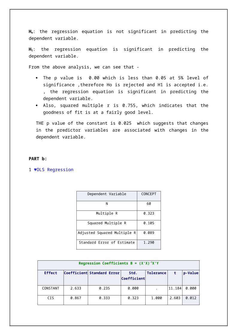
Regression Coefficients B = (X'X)-1X'Y
Effect Coefficient Standard Error Std.Coefficient
Tolerance t p-Value
CONSTANT 2.633 0.235 0.000 . 11.184 0.000
CIS 0.867 0.333 0.323 1.000 2.603 0.012
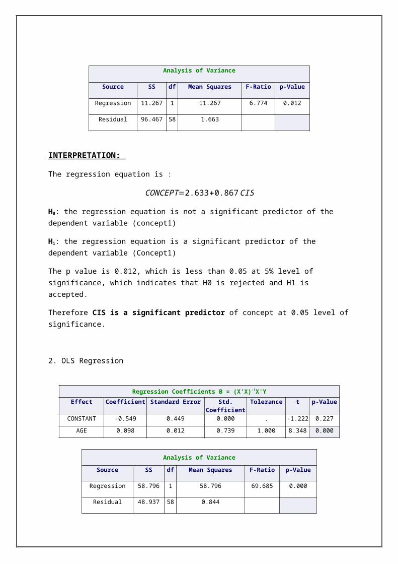
Analysis of Variance
Source SS df Mean Squares F-Ratio p-Value
Regression 11.267 1 11.267 6.774 0.012
Residual 96.467 58 1.663
INTERPRETATION:
The regression equation is :
CONCEPT=2.633+0.867CIS
H0: the regression equation is not a significant predictor of the dependent variable (concept1)
H1: the regression equation is a significant predictor of the dependent variable (Concept1)
The p value is 0.012, which is less than 0.05 at 5% level of significance, which indicates that H0 is rejected and H1 is accepted.
Therefore CIS is a significant predictor of concept at 0.05 level of significance.
2. OLS Regression
Regression Coefficients B = (X'X)-1X'YEffect Coefficient Standard Error Std.
CoefficientTolerance t p-Value
CONSTANT -0.549 0.449 0.000 . -1.222 0.227
AGE 0.098 0.012 0.739 1.000 8.348 0.000
Analysis of Variance
Source SS df Mean Squares F-Ratio p-Value
Regression 58.796 1 58.796 69.685 0.000
Residual 48.937 58 0.844
INTERPRETATION:
The regression equation is: concept=−0.549+0.098 AGE
H0: the regression equation is not a significant predictor of the dependent variable( concept1)
H1: the regression equation is a significant predictor of the dependent variable( Concept1)
The p value is 0.000 , which is less than 0.05 at 5% level of significance ,which indicates that H0 is rejected and H1 is accepted.
Therefore AGE is a significant predictor of concept at 0.05 level of signicance.
3. OLS Regression
Regression Coefficients B = (X'X)-1X'YEffect Coefficient Standard Error Std.
CoefficientTolerance t p-Value
CONSTANT 2.211 0.282 0.000 . 7.851 0.000
MARTIAL 1.253 0.341 0.435 1.000 3.679 0.001
Analysis of Variance
Source SS df Mean Squares F-Ratio p-Value
Regression 20.380 1 20.380 13.532 0.001
Residual 87.353 58 1.506
INTERPRETATION:
The regression equation is: concept=2.211+1.253MARTIAL
H0: the regression equation is not a significant predictor of the dependent variable (concept1)
H1: the regression equation is a significant predictor of the dependent variable ( Concept1)
The p value is 0.001, which is less than 0.05 at 5% level of significance , which indicates that H0 is rejected and H1 is accepted.
Therefore MARTIAL is a significant predictor of concept at 0.05 level of signicance.
4. OLS Regression

Regression Coefficients B = (X'X)-1X'Y
Effect Coefficient Standard Error Std.Coefficient
Tolerance t p-Value
CONSTANT 3.395 0.352 0.000 . 9.633 0.000
NUMCAR -0.195 0.182 -0.139 1.000 -1.073 0.288
Analysis of Variance
Source SS df Mean Squares F-Ratio p-Value
Regression 2.095 1 2.095 1.150 0.288
Residual 105.638 58 1.821
INTERPRETATION:
The regression equation is: concept=3.395−0.195 NUMCAR
H0: the regression equation is not a significant predictor of the dependent variable( concept1)
H1: the regression equation is a significant predictor of the dependent variable( Concept1)
The p value is 0.288 , which is MORE than 0.05 at 5% level of significance ,which indicates that H0 is accepted and H1 is rejected.
Therefore NUMCAR is NOT a significant predictor of concept at 0.05 level of signicance.
5. OLS Regression
Regression Coefficients B = (X'X)-1X'YEffect Coefficient Standard Error Std.
CoefficientTolerance t p-Value
CONSTANT 4.968 0.295 0.000 . 16.856 0.000
AVAGE -1.074 0.150 -0.685 1.000 -7.164 0.000
Analysis of Variance
Source SS df Mean Squares F-Ratio p-Value
Regression 50.576 1 50.576 51.321 0.000
Residual 57.158 58 0.985
INTERPRETATION:
The regression equation is: concept=4.968−1.074 AVAGE

H0: the regression equation is not a significant predictor of the dependent variable( concept1)
H1: the regression equation is a significant predictor of the dependent variable( Concept1)
The p value is 0.000 , which is less than 0.05 at 5% level of significance ,which indicates that H0 is rejected and H1 is accepted.
Therefore AVAGE is a significant predictor of concept at 0.05 level of signicance.
6. OLS Regression
Regression Coefficients B = (X'X)-1X'Y
Effect Coefficient Standard Error Std.Coefficient
Tolerance t p-Value
CONSTANT 2.136 0.166 0.000 . 12.843 0.000
NUMTRIP 0.430 0.053 0.729 1.000 8.116 0.000
Analysis of VarianceSource SS Df Mean Squares F-Ratio p-Value
Regression 57.286 1 57.286 65.863 0.000
Residual 50.447 58 0.870
INTERPRETATION:
The regression equation is: concept=2.136+0 .430NUMTRIP
H0: the regression equation is not a significant predictor of the dependent variable( concept1)
H1: the regression equation is a significant predictor of the dependent variable( Concept1)
The p value is 0.000 , which is less than 0.05 at 5% level of significance ,which indicates that H0 is rejected and H1 is accepted.
Therefore NUMTRIP is a significant predictor of concept at 0.05 level of signicance.
A SIMPLER MODEL (involving fewer predictors) can be developed. This is as follows:
Best Subset Regression:DEPENDENT VARIABLE: CONCEPT

Model No R-Sq Adjusted R-Sq Mallows' Cp MSE Variables
1 0.546 0.538 42.339 0.844 AGE
2 0.532 0.524 45.374 0.870 NUMTRIP
3 0.707 0.696 9.524 0.555 AGE, NUMTRIP
4 0.662 0.650 19.222 0.639 AVAGE, AGE
5 0.754 0.741 1.295 0.474 AVAGE, AGE, NUMTRIP
6 0.709 0.693 11.100 0.561 CIS, AGE, NUMTRIP
7 0.754 0.736 3.190 0.481 AVAGE, MARTIAL, AGE, NUMTRIP
8 0.754 0.736 3.230 0.482 AVAGE, NUMCAR, AGE, NUMTRIP
9 0.755 0.732 5.101 0.489 AVAGE, MARTIAL, NUMCAR, AGE, NUMTRIP
10 0.755 0.732 5.108 0.489 AVAGE, MARTIAL, CIS, AGE, NUMTRIP
11 0.755 0.727 7.000 0.498 NUMTRIP, AVAGE, NUMCAR, MARTIAL, AGE, CIS
Model No AIC AICC BIC Variables
1 164.044 164.473 170.327 AGE
2 165.868 166.296 172.151 NUMTRIP
3 139.824 140.551 148.201 AGE, NUMTRIP
4 148.348 149.076 156.726 AVAGE, AGE
5 131.290 132.401 141.762 AVAGE, AGE, NUMTRIP
6 141.423 142.534 151.894 CIS, AGE, NUMTRIP
7 133.172 134.756 145.738 AVAGE, MARTIAL, AGE, NUMTRIP
8 133.217 134.802 145.783 AVAGE, NUMCAR, AGE, NUMTRIP
9 135.071 137.225 149.731 AVAGE, MARTIAL, NUMCAR, AGE, NUMTRIP
10 135.078 137.232 149.739 AVAGE, MARTIAL, CIS, AGE, NUMTRIP
11 136.956 139.780 153.711 NUMTRIP, AVAGE, NUMCAR, MARTIAL, AGE, CIS
The Best Models:
Criteria Value Best Subset Model
Adjusted R-Sq 0.741 AVAGE, AGE, NUMTRIP

The Best Models:
Criteria Value Best Subset Model
AIC 131.290 AVAGE, AGE, NUMTRIP
AIC (Corrected) 132.401 AVAGE, AGE, NUMTRIP
Schwarz's BIC 141.762 AVAGE, AGE, NUMTRIP
INTERPRETATION:
From the tables above, we see that the adjusted R sq of AVAGE, AGE, NUMTRIP is highest, i.e. 0.741 which indicates that it is the simple and best subset model.The AIC value of AVAGE, AGE, NUMTRIP is 131.290, which is the lowest, hence the best subset.
So, the percentage improvement of the simpler model over the full model would be as follows: [(0.741-0.727)/ 0.727]*100= 1.9257%
QUESTION 3:

Divide the sample into 4 groups: Rushmore – Single, Rushmore – Married, Other Company – Single, and Other Company – Married. Run a single factor ANOVA to test the null hypothesis that the mean of the CONCEPT for the four groups are the same at 5% level of significance? If not which group has the highest average rating?
SOLUTION:
Analysis of VarianceEffects coding used for categorical variables in model.
The categorical values encountered during processing are
Variables Levels
GROUPS (4 levels) 1.000 2.000 3.000 4.000
Dependent Variable CONCEPT
N 60
Multiple R 0.563
Squared Multiple R 0.317
Analysis of Variance
Source Type III SS df Mean Squares F-Ratio p-Value
GROUPS 34.150 3 11.383 8.663 0.000
Error 73.583 56 1.314
INTERPRETATION:
LET US ASSUME:Ho: the mean of the CONCEPT for the four groups are the same.H1: the mean of the CONCEPT for the four groups are different. From the analysis of variance, we get to know that p value is 0.000 at 5% level of significance ,which is less than 0.05.therefore null hypothesis is rejected and alternate hypothesis is accepted. We interpret that at least one of the means is different.
Now to know which mean is different, we need to perform the pairwise comparison, PAIRWISE COMPARISON:Post Hoc Test of CONCEPT

Using least squares means.
Using model MSE of 1.314 with 56 df.
Tukey's Honestly-Significant-Difference Test
GROUPS(i) GROUPS (j) Difference p-Value 95% Confidence Interval
Lower Upper
1 2 -0.569 0.560 -1.719 0.581
1 3 0.148 0.992 -1.263 1.558
1 4 -1.727 0.001 -2.848 -0.606
2 3 0.717 0.454 -0.562 1.996
2 4 -1.158 0.011 -2.109 -0.207
3 4 -1.875 0.001 -3.128 -0.622
INTERPRETATION:
We compare the p value of all the 6 groups and select those p values whose value is less than 0.05.
From the above table, p values of group (1,4) , (2,4),( 3,4) are less than 0.05.
Amongst the group , we get to know that variable 4 (rushmore married) is common in all the groups having p value less than 0.05.
Therefore , it means that the mean of RUSHMORE MARRIED(4) is different .
QUESTION 4:
Divide the NUMCAR as follows – One and More than One. Now using the CONCEPT and the 4 groups (as developed in 3 above) run a 2 way ANOVA with the second concept as NUMCAR groups. Is there any difference between the results obtained in 3 above and this new 2 way ANOVA at 5% level of significance?
SOLUTION:

Analysis of Variance
Effects coding used for categorical variables in model.
The categorical values encountered during processing are
Variables Levels
GROUPS (4 levels) 1.000 2.000 3.000 4.000
NUMCAR1 (2 levels) 0.000 1.000
Dependent Variable CONCEPT
N 60
Multiple R 0.593
Squared Multiple R 0.351
Analysis of Variance
Source Type III SS df Mean Squares F-Ratio p-Value
GROUPS 34.538 3 11.513 8.568 0.000
NUMCAR1 2.614 1 2.614 1.945 0.169
GROUPS *NUMCAR1 2.430 3 0.810 0.603 0.616
Error 69.873 52 1.344
INTERPRETATION:
We run a two way annova with the 4 GROUPS and NUMCAR.Let us assume, Hog: the average means of CONCEPT is similar as the average means of GROUPS.H1 g: the average means of CONCEPT is different from the average means of GROUPS.
Ho n: the average means of CONCEPT is similar as the average means of NUMCARH1 n: the average means of CONCEPT is different from the average means of NUMCAR. From the p values, we can see the null hypothesis (ho g) is rejected due to its value being less than 0.05, which means that the average means of CONCEPT is different from the average means of GROUPS.

Similarly, the p value of NUMCAR is greater than 0.05, therefore we accept the null hypothesis( ho n), i.e. , the average means of CONCEPT is similar as the average means of NUMCAR.
Now to know which variable of the GROUP has a different mean, we perform a pairwise comparison of the GROUPS.
PAIRWISE COMPARISON
Post Hoc Test of CONCEPTUsing least squares means.Using model MSE of 1.344 with 52 df.
Tukey's Honestly-Significant-Difference Test
Groups I) Groups (J) Difference p-Value 95% Confidence Interval
Lower Upper
1 2 -0.615 0.529 -1.781 0.550
1 3 0.089 0.998 -1.340 1.519
1 4 -1.786 0.001 -2.922 -0.650
2 3 0.705 0.483 -0.592 2.001
2 4 -1.170 0.012 -2.134 -0.207
3 4 -1.875 0.001 -3.145 -0.605
INTERPRETATION:
We compare the p value of all the 6 groups and select those p values whose value is less than 0.05.
From the above table, p values of group (1,4) , (2,4),( 3,4) are less than 0.05.
Amongst the group , we get to know that variable 4 (Rushmore Married) is common in all the groups having p value less than 0.05.
Therefore , it means that the mean of RUSHMORE MARRIED(4) is different .
Therefore, there is no difference in the results obtained in question 3 above and this new 2 way ANOVA at 5% level of significance.
QUESTION 5:

Factor analyse the full 60x7 data matrix using principal component analysis using Varimax rotation. Apply Kaiser’s criterion (eigenvalue > 1) to extract the principal components. How will you interpret each set of rotated factor loadings?
▼Factor Analysis
Latent Roots (Eigenvalues)
1 2 3 4 5 6 7
3.413 1.065 0.913 0.663 0.432 0.353 0.161
Component Loadings
1 2
CONCEPT 0.906 -0.014
CIS 0.460 0.496
AGE 0.855 0.100
MARTIAL 0.619 0.075
NUMCAR -0.207 0.853
AVAGE -0.779 0.269
NUMTRIP 0.786 0.048
Variance Explained by Components
1 2
3.413 1.065
Percent of Total Variance Explained
1 2
48.754 15.217

Rotated Loading Matrix (VARIMAX, Gamma = 1.000000)
1 2
CONCEPT 0.904 -0.051
CIS 0.481 0.477
AGE 0.858 0.065
MARTIAL 0.621 0.049
NUMCAR -0.171 0.861
AVAGE -0.767 0.301
NUMTRIP 0.788 0.015
"Variance" Explained by Rotated Components
1 2
2.791 1.063
Percent of Total Variance Explained
1 2
39.871 15.182
INTERPRETATION:
There are two latent factors at work which explains 63.97% of the total market behaviour of the rushmore insurance.
P1=0.906CONCEPT+0.460CIS+0.855 AGE+0.619MARTIAL−0.207 NUMCAR−0.779 AVAGE+0.786 NUMTRIP
P2=−0.014CONCEPT +0.496CIS+0.100 AGE+0.075MARTIAL+0.853 NUMCAR+0.269 AVAGE+0.048NUMTRIP
FACTORS PRINCIPAL COMPONENTS
CONCEPT 1

CIS 1AGE 1
MARTIAL 1NUMCAR 1AVAGE 2
NUMTRIP 1
Nomenclature of PC1 consisting of factors- CONCEPT, CIS, AGE, MARTIAL, AVAGE, NUMTRIP is
“SELF CHARACTERISTICS”
Nomenclature of PC2 consisting of factors- NUMCAR is
“USAGE CHARACTERISTICS”
Therefore we can say that 48.754% of market would buy insurance depending on self characteristics and 15.21% of market would buy insurance depending on the car characteristics.
RECOMMENDATIONS:
1.WISDOM OF OFFERING :
From the CHI SQUARE test of association, we understood that the association between interest in the policy and the current insurance supplier is very strong and significant, which means that the policy would be acceptable by the majority of respondents.
2. TARGET MARKET:
The factors influencing the respondent to buy the insurance are:
The age of the respondents, The marital status, Average age of cars owned The number of trips taken by the car owned
Tukey's Honestly-Significant-Difference TestAGE1(i) AGE1(j) Difference p-Value 95% Confidence Interval
Lower Upper1 2 -0.932 0.022 -1.762 -0.1031 3 -1.991 0.000 -2.821 -1.1621 4 -2.883 0.000 -4.054 -1.7132 3 -1.059 0.010 -1.921 -0.1962 4 -1.951 0.000 -3.145 -0.7573 4 -0.892 0.208 -2.086 0.302
The coding of age were as follows:

20-30: 1 30-40: 2 40-50: 3 50 and above : 4
After the pairwise comparison, we can see that AGE GROUP 20-40 is the segment highly interested in the insuance policy.
Also, from the above analysis, (question 4) , we concluded that the RUSHMORE MARRIED group is the most significant group and therefore this segment can serve as the target market of the insurance company.
From the factor analysis, we saw that 84.96% of market would buy insurance depending on self characteristics and 12.948% of market would buy insurance depending on the car characteristics.
3.FURTHER RESEARCH REQUIRED:
Cluster analysis could be done to segment the market further more.