Bayesian Treed Models

by

Hugh Chipman, Edward I. George and Robert E. McCulloch 1

University of Waterloo, University of Texas at Austin and University of Chicago

February 2001

Abstract

When simple parametric models such as linear regression fail to adequately approximate a

relationship across an entire set of data, an alternative may be to consider a partition of the

data, and then use a separate simple model within each subset of the partition. Such an alterna-

tive is provided by a treed model which uses a binary tree to identify such a partition. However,

treed models go further than conventional trees (eg CART, C4.5) by �tting models rather than

a simple mean or proportion within each subset. In this paper, we propose a Bayesian approach

for �nding and �tting parametric treed models, in particular focusing on Bayesian treed regres-

sion. The potential of this approach is illustrated by a cross-validation comparison of predictive

performance with neural nets, MARS, and conventional trees on simulated and real data sets.

Keywords: binary trees, Markov chain Monte Carlo, model selection, stochastic search.

1Hugh Chipman is Associate Professor, Department of Statistics and Actuarial Science, University of Waterloo,

Waterloo, ON N2L 3G1, hachipman@uwaterloo.ca. Edward I. George holds the Ed and Molly Smith Chair in

Business Administration and is Professor of Statistics, Department of MSIS, University of Texas, Austin, TX 78712-

1175, egeorge@mail.utexas.edu, and Robert E. McCulloch is Professor of Statistics, Graduate School of Business,

University of Chicago, IL 60637, robert.mcculloch@gsb.uchicago.edu. This work was supported by NSF grant DMS

9803756, Texas ARP grant 003658690, the Natural Sciences and Engineering Research Council of Canada, the

Mathematics of Information Technology and Complex Systems (MITACS), and research funding from the Graduate

Schools of Business at the University of Chicago and the University of Texas at Austin. The authors would like to

acknowledge and thank the reviewers for their many valuable suggestions.

1 Introduction

Parametric models such as linear regression can provide useful, interpretable descriptions of simple

structure in data. However, sometimes such simple structure does not extend across an entire data

set and may instead be con�ned more locally within subsets of the data. In such cases, the simple

structure might be better described by a model that partitions the data into subsets and then uses

separate submodels for the subsets of the partition. In this paper, we explore the use of \treed

models" to describe such structure.

Basically, treed models are an elaboration of conventional tree models that use binary trees to

partition the data into \homogeneous" subsets where the response can be described by a simple

mean or proportion. Although such models can provide a useful approach to handling interactions

and nonlinearities, they do not fully exploit partitions with more substantial statistical structure

within the subsets. To overcome this limitation, treed models are constructed so that the model

structure, as opposed to the data, is homogeneous within a terminal node. This allows richer

submodels for each of the subsets of the tree-determined partition.

The main thrust of this paper is to propose and illustrate a Bayesian approach to �nding and

�tting treed models. In particular, we pay special attention to treed regressions, where linear

regression models are used to describe the variation within each of these subsets. Alexander and

Grimshaw (1996) coined the term \treed regression" to refer to a tree with simple linear regression

in each terminal node. We adopt this terminology to include treed models with multiple regressions,

and refer to our approach as Bayesian treed regression.

The idea of treed models is not new. Karali�c (1992) considered multiple regression models

in the terminal nodes, in conjunction with a greedy grow/prune algorithm. Quinlan's (1992) M5

algorithm also �ts models of this form, but linear models were added to a conventional tree as part

of the pruning stage. Torgo (1997) uses linear models, k-nearest neighbors, or kernel regressors in

terminal nodes, but also adds these to a conventional tree after growing. Chaudhuri, Huang, Loh,

and Yao (1994) consider trees with linear models (with possible polynomial terms) in the terminal

nodes. Chaudhuri, Lo, Loh, and Yang (1995) extend this idea to non-normal response models. Loh

(2001) also considers linear regressions in terminal nodes, and attempts to correct for possible bias

in selection of splits. Waterhouse, MacKay, and Robinson (1996) consider a tree-structured mixture

of experts model, in which the individual experts are linear models. Unlike the other treed models,

the predictors are not used to specify what expert is used for a particular data point; rather mixing

1

probabilities inferred from the data are used.

The Bayesian approach proposed here is substantially di�erent from this past work. These

earlier approaches are based on using some kind of greedy algorithm for tree construction, growing

a large tree and then pruning it back. In contrast, the Bayesian approach induces a posterior

distribution that can be used to guide a stochastic search towards `more promising' treed models,

thereby more fully exploring the model space. Such a Bayesian approach was successfully applied

to conventional CART trees by Chipman, George, and McCulloch (1998) (hereafter denoted CGM)

and Denison, Mallick, and Smith (1998). The Bayesian approach here elaborates this work { replac-

ing the terminal node means or class probabilities in a conventional trees with more sophisticated

models such as linear regression. The form of the terminal node models then becomes an integral

part of the stochastic search, as the posterior is based on both the tree structure and terminal

node models. The Bayesian approach also provides added exibility for submodel speci�cation.

For example, the possibility of using di�erent error variances for subset models, notably absent in

previous methods, is easily accommodated.

A key aspect of any Bayesian approach is the introduction of prior distributions on all the

unknowns, here the tree structures and terminal node models. In this paper we propose a class

of priors and recommend speci�c \default" choices from within this class. We argue that, while

no guarantees are made, these priors should lead to good results in a variety of problems and we

illustrate this in the examples. Our prior plays two important roles in our methodology. First

and foremost it provides a \penalty" to avoid over�tting in a natural, interpretable way. Secondly

shrinkage of the bottom node parameters toward reasonable values stabilizes the estimation. Be-

cause treed model classes are so large, these aspects are critically important for obtaining realistic

�ts and predictions.

In Section 2, treed models are presented in a mathematical framework, and the important

special case of treed regressions outlined and introduced via an example. Priors applicable to treed

models of any form are discussed in Section 3.1. The search for interesting models is part of the

Markov chain Monte Carlo method for estimating the posterior, discussed in Section 3.2. For

treed regressions, the particular case considered here, prior parameters are selected in Section 4, in

such a way that reasonable automatic choices of prior parameters can be made. In Section 5, two

simulated and one real dataset are used to evaluate the predictive accuracy of treed regressions,

and four competing models. We conclude in Section 6 with a discussion of directions for future

investigations.

2

2 Treed Models

2.1 The General Model

Suppose we are interested in modeling the relationship between a variable of interest Y and a set

of potential explanatory variables (a feature vector) x. A treed model is a speci�cation of the

conditional distribution of Y jx consisting of two components - a binary tree T that partitions the

x space, and a parametric model for Y that is associated with each subset of the partition.

The binary tree T is the conventional tree associated with CART (Breiman, Friedman, Olshen,

and Stone (1984)). Each interior node of the tree splits into two children, using a single predictor

variable in the splitting rule. For ordered predictors, the rule corresponds to a cutpoint. For

categorical predictors, the set of possible categories is partitioned into two sets. The tree T has

b terminal nodes with each terminal node corresponding to a region in the space of potential x

vectors. The b regions corresponding to the b terminal nodes are disjoint so that the tree partitions

the x space by assigning each value of x to one of the b terminal nodes.

The treed model then associates a parametric model for Y at each of the terminal nodes of

T . More precisely, for values x that are assigned to the ith terminal node of T , the conditional

distribution of Y jx is given by a parametric model Y jx � f(yjx; �i) with parameter �i. Letting

� = (�1; : : : ; �b), a treed model is fully speci�ed by the pair (�; T ). It may be of interest to note

that early tree formulations such as CART were essentially proposed as data analysis tools rather

than models. By elaborating the formulation as a parametric model, we set the stage for a Bayesian

analysis. By treating the training sample (y; x) as realizations from a treed model, we can then

compute the posterior distribution over (�; T ).

CGM and Denison et. al. (1998) discuss Bayesian approaches to the CART model. In those

papers, the terminal node distributions of Y , f(yjx; �), do not depend on x. For example, a

Bayesian version of a conventional regression tree is obtained by letting � = (�; �) and f(yjx; �) =

N(�; �2). The conditional distribution of Y given x is then Y jx � N(�i; �2i ) when x is assigned

to the terminal node associated with �i = (�i; �i). Such models correspond to step functions for

the expected value of Y jx, and may require large trees to approximate an underlying distribution

Y jx whose mean is continuously changing in x. By using a richer structure at the terminal nodes,

the treed models in a sense transfer structure from the tree to the terminal nodes. As a result, we

expect that smaller, and hence more interpretable, trees can be used to describe a wider variety of

distributions for Y jx.

3

Finally, we should point out that although we use the one symbol \x" for notational simplicity,

we may decide, a priori, to use one subset of the components of x in the rules de�ning the binary

tree T and another subset in the �tting the models p(yjx; �). These subsets need not be disjoint.

2.2 Treed Regression: An Example

One of the most familiar and useful parametric models is the linear model with normal error:

Y jx � N(x0�; �2). A treed regression is readily obtained by incorporating this model into our treed

model framework. Simply let �i = (�i; �i) and associate Y jx � N(x0�i; �2i ) with the terminal node

corresponding to x. We also assume that given the x values, the Y values are independent of each

other. Note that this treed regression allows both �i and �i to vary from node to node. This allows

us to exibly �t both global non-linearity and global heteroskedasticity.

In subsequent sections, we describe in detail a Bayesian approach for �nding and �tting treed

regressions to data. In particular, in Section 5.3, we illustrate the performance of our approach

on the well-known Boston Housing data, Harrison and Rubinfeld (1978). To give the reader an

immediate sense of the potential of our approach, we describe here some of what we found.

The data consist of 14 characteristics of 506 census tracts in the Boston area. The response

is the logged median value of owner occupied homes in each tract, and is listed in Table 1, along

with the 13 predictor variables. One of the treed regressions that was selected by the Bayesian

stochastic search is described by Figures 1 and 2. Details of the Bayesian formulation such as prior

choices that led to this model are discussed in Section 5.3.

Our �tted treed regression has 6 terminal nodes depicted in Figure 1. One node that is imme-

diately of interest is node 4, which has substantially larger residual standard deviation than the

other nodes. This node consists of tracts with high tax rates (137 of the regions have taxes this

high), and small distance to employment centres (105 of all tracts have this low a score, and 73 of

the tracts with tax above 469). Among the high-tax, downtown areas, there appears to be more

variation in the log median house price. Evidently, this is variation that is not readily explained by

any predictors, and the treed regression search elects to leave the data alone, rather than over�t it.

The data at each of the 6 terminal nodes of our �tted treed regression is described by a separate

regression with 14 estimated coeÆcients (including an intercept). As shown in Figure 2, the coef-

�cient of each predictor varies from terminal node to terminal node, re ecting varying sensitivity

of the response to the predictors. Note that in �tting this treed regression, we �rst standardized

all the predictors (see section 4), so that all can be compared on the same scale in Figure 2. The

4

Name Description Min Max

CRIM per capita crime rate by town 0.006 88.976

ZN proportion of residential land zoned for lots over

25,000 sq.ft.

0.000 100.000

INDUS proportion of non-retail business acres per town 0.460 27.740

CHAS Charles River dummy variable (= 1 if tract

bounds river; 0 otherwise)

0.000 1.000

NOX nitric oxides concentration (parts per 10 million) 0.385 0.871

RM average number of rooms per dwelling 3.561 8.780

AGE proportion of owner-occupied units built prior to

1940

2.900 100.000

DIS weighted distances to �ve Boston employment

centres

1.130 12.126

RAD index of accessibility to radial highways 1.000 24.000

TAX full-value property-tax rate per $10,000 187.000 711.000

PTRATIO pupil-teacher ratio by town 12.600 22.000

B 1000(Bk � 0:63)2 where Bk is the proportion of

blacks by town

0.320 396.900

LSTAT % lower status of the population 1.730 37.970

MEDV Log Median value of owner-occupied homes in

$1000's

1.609 3.912

Table 1: Variables in the Boston dataset

5

Tax: 469

Nox: 0.5100

Nox: 0.4721

Node 1 n=155, s=0.0324

Node 2 n=62, s=0.0294

Node 3 n=152, s=0.0461

Dis: 1.97

Node 4 n=73, s=0.1006

Age: 71.6

Node 5 n=12, s=0.0348

Node 6 n=52, s=0.0438

Figure 1: The tree structure of the treed regression model for the Boston data. Each node is

represented by a line of text. Non-terminal nodes indicate the name of the splitting variable, and

the cutpoint of the split. The �rst line after a nonterminal node is the child node with all values

� the split value. In terminal nodes, the number of data points in the node (n), and the residual

standard deviation (s) are given. Note that the units of split variables are on the original scale.

6

11

1 1 1 1

1

1 11

1 1

1

1

−1.

5−

1.0

−0.

50.

00.

5

Estimated coefficients by terminal node (1−6)

beta

22

2 2

2 2

2

2 2

2

2

2

22

3

3

3 33

3

3

33

3

3 3

3

34

4

4

4

4

4

4

4

4

4

44 4

4

5

5

5 5 55

5

5

5

5 5 5

5

56

6

6 6 6 66

6

66 6 6

6

6

inte

rcep

t

CR

IM

ZN

IND

US

CH

AS

NO

X

RM

AG

E

DIS

RA

D

TA

X

PT

RA

TIO

B

LST

AT

Figure 2: Regression coeÆcient estimates of the treed model for the Boston data. Estimates for

a regression in a speci�c node are linked by lines and labeled by node number. CoeÆcients for

di�erent variables may be plotted on the same scale because in the regression models coeÆcients

are scaled equally.

7

coeÆcients in node 4 for NOX and DIS are very di�erent from other nodes. Recall that this node

contains the close to downtown, high tax areas. The large negative coeÆcients mean that these

tracts are more sensitive to NOX and DIS than other tracts. Speci�cally, high pollution and larger

distance from city centers will decrease the median value of a house much more than in other tracts.

A possible explanation is that people may walk or take public transport because of their proximity

to work, and so a relatively small increase in distance could a�ect value. Other interesting patterns

include the coeÆcients for crime rate (CRIM). In nodes 1-3, which are low property tax areas,

the e�ect of crime is zero or small. In the remaining three nodes, where taxes are higher, the

coeÆcients are negative, implying that increasing crime rates decrease value. Again, some tracts

are more sensitive to this variable than others.

3 A Bayesian Approach for Treed Modeling

In a nutshell, the Bayesian approach to model uncertainty problems proceeds as follows. The

uncertainty surrounding the space of possible models is described by a prior distribution p(model).

Based on the observed data, the posterior distribution on the model space is p(model j data) /

p(data j model) p(model). Under the chosen prior, the best candidates for selection are then the

high posterior probability models. Although simple to state, the e�ective implementation of this

Bayesian approach can be delicate matter. The two crucial steps are the meaningful choice of

prior distributions, and a method for identi�cation of the high posterior models. We now describe

methods for accomplishing each of these steps for general treed model classes.

3.1 Prior Formulations for Treed Models

Since a treed model is identi�ed by (�; T ), a Bayesian analysis of the problem proceeds by specifying

a prior probability distribution p(�; T ). This is most easily accomplished by specifying a prior p(T )

on the tree space and a conditional prior p(�jT ) on the parameter space, and then combining them

via p(�; T ) = p(�jT )p(T ).

For p(T ), we recommend the speci�cation proposed in CGM for conventional trees. This prior is

implicitly de�ned by a tree-generating stochastic process that \grows" trees from a single root tree

by randomly \splitting" terminal nodes. A tree's propensity to grow under this process is controlled

by a two-parameter node splitting probability Pr(node splitsjdepth = d) = �(1 + d)�� , where the

root node has depth 0. The parameter � is a \base" probability of growing a tree by splitting a

8

1 2 3 4 5 6

050

010

0020

00

prior 1

2 4 6 8 10 12

020

060

010

0014

00

prior 2

2 4 6 8

050

010

0020

00

prior 3

2 4 6 8 10 12

050

010

0020

00

prior 4

Figure 3: Marginal prior distribution for the number of terminal nodes, under various settings of �

and �. Values for (�; �) are: upper left = (:5; 2), upper right = (:95; 1), lower left = (:5; 1), lower

right = (:5; :5).

current terminal node and � determines the rate at which the propensity to split diminishes as

the tree gets larger. For details, see CGM. Figure 3 displays the marginal prior distribution on

the number of terminal nodes (the tree size) for 4 di�erent settings of (�; �). (These �gures are

histograms of the tree sizes obtained by repeated simulation of trees from p(T )). Using such �gures

as a guide, values of (�; �) can be chosen to, for example, express the belief that reasonably small

trees should yield adequate �ts to the data. The tree prior p(T ) is completed by specifying a prior

on the splitting rules assigned to intermediate nodes. We use a prior that is uniform on available

variables at a particular node, and within a given variable, uniform on all possible splits for that

variable.

Turning to the speci�cation of p(�jT ), we note that while p(T ) above is suÆciently general for

9

all treed model problems, the speci�cation of p(�jT ) will necessarily be tailored to the particular

form of the model p(yjx; �) under consideration. This will been seen in Section 4 where we provide

a detailed discussion of prior speci�cation for the treed regression model. However, some aspects of

p(�jT ) speci�cation should be generally considered. When reasonable, an assumption of indepen-

dent and identically distributed (iid) components of � reduces the choice to that of a single density

p(�). However, even with this simpli�cation, the speci�cation of p(�) can be both diÆcult and

crucial. In particular, a key consideration is to avoid con ict between p(�jT ) and the likelihood

information from the data. On the one hand, if we make p(�) too tight (ie with very small spread

around the prior mean) the prior may be too informative and overwhelm the information in the

data corresponding to a terminal node. On the other hand, if p(�) is too di�use (spread out),

p(�jT ) will be even more so, particularly for large values of b (large trees) given our iid model for

the �i. Very spread out priors can \wash out" the likelihood in the sense of the Bartlett-Lindley

paradox, Bartlett (1957). Thus, choice of an excessively di�use prior will push the posterior of T

towards concentrating on small trees. As will be seen in Section 4, both training data information

and prior beliefs can be very useful for avoiding such pitfalls.

3.2 Markov Chain Monte Carlo Posterior Exploration

Given a set of training data, the Bayesian analysis would ideally proceed by computing the entire

posterior distribution of (�; T ). Unfortunately, in problems such as this, the size of the model space

is so large that complete calculation of the posterior is infeasible. However, posterior information

can still be obtained by using a combination of limited analytical simpli�cation together with

indirect simulation sampling from the posterior via Markov chain Monte Carlo (MCMC) methods.

In particular, the Markov chain simulation can be used as a stochastic search algorithm which

seems to be more comprehensive than traditional greedy grow/prune algorithms.

Our algorithm has the potential to be more more comprehensive in three important ways. First,

the stochastic steps help move the search past local maxima. Second, in addition to grow/prune

steps we use \swap" and \change" steps which help �nd better trees. Finally, repeated restarting of

the chain identi�es a more diverse set of trees. These ideas were �rst developed in CGM, in the con-

text of conventional trees. There, simulation studies illustrated that stochastic search, change/swap

steps and multiple restarts found better trees than a greedy search. Chipman et. al. (2001) also

showed that this MCMC algorithm can �nd a wider variety of trees than a bootstrapped greedy

grow/prune algorithm. Lutsko and Kuijpers (1994) considered a MCMC-like approach using sim-

10

ulated annealing, and also found improvements.

In its essentials, the method we use is the same as that in CGM. Our �rst step is to simplify the

problem by integrating � out of the posterior so only T remains. Given T , we index the observed

data so that (yij ; xij) is the jth observation amongst the data such that xij corresponds to the i

th

node. Let ni denote the number of observations corresponding to the ith node and let (Y;X) denote

all of the training data. Then,

p(Y jX; T ) =

Zp(Y jX;�; T )p(�jT)d�

=bY

i=1

Z niYj=1

p(yij jxij ; �i)p(�i)d�i (1)

where the second equality follows from the assumed conditional independence of the y0s given the

x0s and the modeling of the �i as iid given T . Note that in the �rst line we assume that X and �

are independent given T , so that the prior on each �i does not depend on the xij values.

We use MCMC to stochastically search for high posterior trees T by using the following

Metropolis-Hastings algorithm which simulates a Markov chain T 0; T 1; T 2; : : : with limiting dis-

tribution p(T jY;X). Starting with an initial tree T 0, iteratively simulate the transitions from T i

to T i+1 by the two steps:

1. Generate a candidate value T � with probability distribution q(T i; T �).

2. Set T i+1 = T � with probability

�(T i; T �) = min

(q(T �; T i)

q(T i; T �)

p(Y jX; T �)p(T �)

p(Y jX; T i)p(T i); 1

): (2)

Otherwise, set T i+1 = T i.

In (2), p(Y jX; T ) is obtained from (1), and q(T; T �) is the kernel which generates T � from T by

randomly choosing among four steps:

� GROW: Randomly pick a terminal node. Split it into two new ones by randomly assigning

it a splitting rule from the prior.

� PRUNE: Randomly pick a parent of two terminal nodes and turn it into a terminal node by

collapsing the nodes below it.

� CHANGE: Randomly pick an internal node, and randomly reassign it a splitting rule from

the prior.

11

� SWAP: Randomly pick a parent-child pair which are both internal nodes. Swap their splitting

rules unless the other child has the identical rule. In that case, swap the splitting rule of the

parent with that of both children.

CGM note that chains simulated by this algorithm tend to quickly gravitate towards a region

where P (T jY;X) is large, and then stabilize, moving locally in that region for a long time. Evidently,

this is a consequence of a proposal distribution which makes local moves over a sharply peaked

multimodal posterior. Some of these modes will be better than others, and it is desirable to visit

more than one. To avoid wasting time waiting for mode-to-mode moves, CGM recommend search

with multiple restarts of the algorithm, saving the most promising trees from each run.

By �tting parametric models relating y to x in each terminal node we hope to obtain good �t

with much smaller trees than in the model considered by CGM. With smaller trees the MCMC

method is better able to explore the space so that the approach is much more computationally

stable. In fact, we have found that fewer restarts and iterations are typically needed here to �nd

high posterior probability trees than in CGM. The decision of how many restarts and runs per start

will vary according to sample size, signal to noise ratio, and complexity of the data.

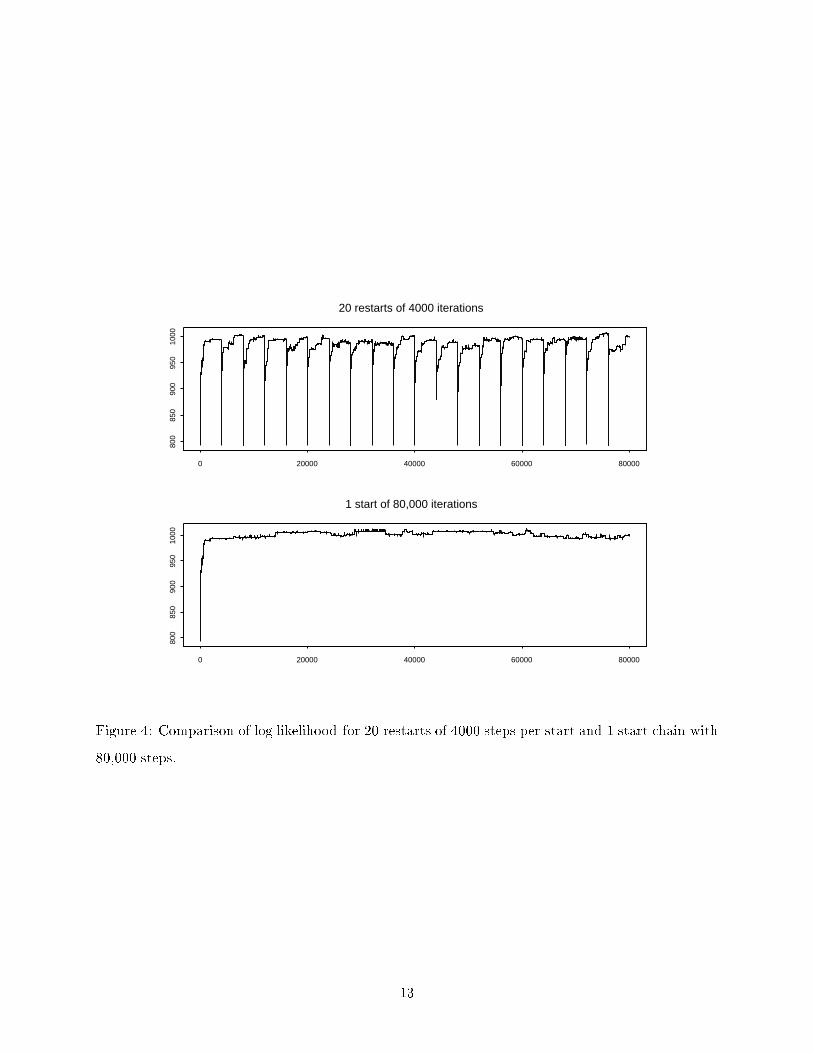
Because MCMC performance is apt to vary from problem to problem, our strategy has been to

use the data to choose the number of restarts and iterations informally. We �rst run some initial

exploratory chains to get a rough idea of how many iterations it takes the chain to get to the point

where the likelihood has stabilized and only small local moves are being made. We then repeatedly

run the chain, restarting it after this number of iterations. Figure 4 illustrates this process for

the data considered in detail in Section 5.3. The top panel displays the log integrated likelihood

(logged values of p(Y jX; T )) for the sequence of trees visited by 20 restarts of 4000 iterations. We

see that within each restarted sequence, the values typically increase dramatically at �rst and then

start to level o� suggesting small local moves. Notice that not all sequences plateau at the same

level, indicating that the algorithm may not be mixing well, and may be getting stuck in local

maxima. The lower panel shows one long run of 80,000 iterations. While additional iterations do

�nd larger values, the bulk of the gain occurs early in the run. In this example either approach

(20 short runs or one long run) would likely yield comparable results. As discussed in CGM and

Denison et. al.(1998), other strategies may be considered, and we are currently engaged in research

directed at this issue.

12

0 20000 40000 60000 80000

800

850

900

950

1000

20 restarts of 4000 iterations

0 20000 40000 60000 80000

800

850

900

950

1000

1 start of 80,000 iterations

Figure 4: Comparison of log likelihood for 20 restarts of 4000 steps per start and 1 start chain with

80,000 steps.

13

4 Speci�cation of p(�jT ) for Treed Regression

In this section we discuss particular parameter prior p(�jT ) speci�cations for the treed regression

model described in Section 2.2. Coupled with the tree prior p(T ) recommended in Section 3.1, such

p(�jT ) completes the prior speci�cation for treed regression. Alternative approaches to p(�jT )

speci�cation that may also warrant consideration are brie y discussed in Section 6.

We begin with the simplifying assumption of independent components �i = (�i; �i) of �, reduc-

ing the speci�cation problem to a choice of p(�; �) for every component (i.e. terminal node). For

this, we propose choosing the conjugate form p(�; �) = p(�j�)p(�) with:

�j� � N(��; �2A�1); �2 ���

�2�(3)

so that the integral (1) of Section 3.2 can be performed analytically (see, for example, Zellner

(1971)). This further reduces the speci�cation problem to the choice of values for the hyperparam-

eters �, �, �� and A.

Before going into the speci�cation details for these hyperparameters, we note in passing that

methods that exibly �t data typically have \parameters" that must be chosen. For example, in

�tting a neural net one must choose a decay parameter. Often these parameters are related to

penalties for model size to avoid over�tting. Models that are too large will have good training

sample �t but poor test sample predictive performance. To some extent, both the choice of our

prior on T (indexed by the two scalar parameters � and �, see Section 3.1) and the choice of the

conjugate prior are related to the issue of penalizing overly large models. Our goal is to choose

a single (or at least small) set of possible hyperparameter values such that the resulting choice of

model works reasonably well in a variety of situations.

As noted in Section 3.1, the choice of this prior is a crucial part of the method. What is

needed is a reasonably automatic way to specify a prior that is neither too tight nor too spread

out. Furthermore, if the results are very sensitive to this choice then the method will not be of

practical use. As will be seen below, our approach to hyperparameter selection makes use of a

rough combination of training data information and prior beliefs, and is similar in spirit to the

prior selection approach of Raftery, Madigan, and Hoeting (1997).

We begin by standardizing the training data by a linear transformation so that each x and y

has an average value of 0 and a range of 1. The purpose of this standardization is to make it easier

to intuitively gauge parameter values. For example, with the standardized data, 2.0 would be a

very large regression coeÆcient because a half range increase in the corresponding predictor would

14

0.0 0.2 0.4 0.6 0.8 1.0

010

000

2000

030

000

4000

0

prior for sigma

Figure 5: Prior distribution for residual variance �2, Boston Housing data.

result in a full range increase in y.

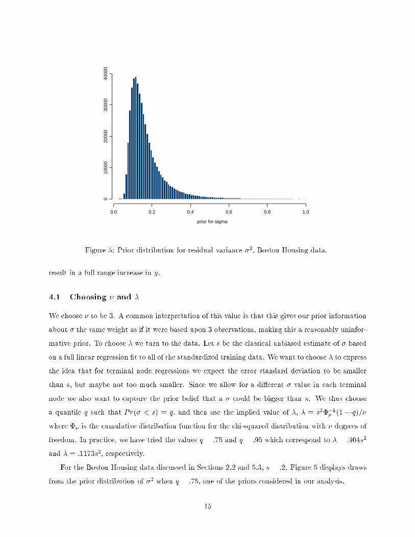
4.1 Choosing � and �

We choose � to be 3. A common interpretation of this value is that this gives our prior information

about � the same weight as if it were based upon 3 observations, making this a reasonably uninfor-

mative prior. To choose � we turn to the data. Let s be the classical unbiased estimate of � based

on a full linear regression �t to all of the standardized training data. We want to choose � to express

the idea that for terminal node regressions we expect the error standard deviation to be smaller

than s, but maybe not too much smaller. Since we allow for a di�erent � value in each terminal

node we also want to capture the prior belief that a � could be bigger than s. We thus choose

a quantile q such that Pr(� < s) = q, and then use the implied value of �, � = s2��1� (1 � q)=�

where �� is the cumulative distribution function for the chi-squared distribution with � degrees of

freedom. In practice, we have tried the values q = :75 and q = :95 which correspond to � = :404s2

and � = :1173s2, respectively.

For the Boston Housing data discussed in Sections 2.2 and 5.3, s = :2. Figure 5 displays draws

from the prior distribution of �2 when q = :75, one of the priors considered in our analysis.

15

4.2 Choosing �� and A

In the absence of prior information, we set �� = 0, the neutral choice indicating indi�erence between

positive and negative values of the components of �. A prior mean of zero on the intercept is

especially plausible because of our standardization of predictors and response to have mean 0.

Of course, given T , the average value of a variable using only those observations at a particular

terminal node may di�er from 0. To accommodate this possibility it will be important to make the

spread of the prior (de�ned by A) broad enough.

To chooseA, we �rst make the simplifying restriction thatA = aI , where I is the identity matrix.

Making A diagonal is a simplifying assumption, though the use of common diagonal element a seems

at least partly justi�ed by the standardization. We choose a, the remaining unknown, by choosing c

such that Pr(�c < � < c) = :95, and then using the relationship a = �3:182=c2 (each component of

� is marginally � t�p�=a, where t� is the t distribution with � degrees of freedom). The constant

3.18 corresponds to the 95% cuto� for a t distribution with � = 3 degrees of freedom.

How do we choose c? Given the standardization we can argue that �1 is a reasonable range

for a coeÆcient since a value of 1 indicates that all the variation in y could be explained by a

single x. However, such reasoning is clearly awed in at least two ways. First of all, given a

tree T the observations corresponding to that node are no longer standardized (although they

would have a range less than 1, and a mean between -1 and 1). Indeed, the whole point of the

model is that the coeÆcients may vary substantially from node to node. Secondly, the presence of

multicollinearity throws all such reasoning out the window. Even with standardized data, the MLE

of a coeÆcient could be arbitrarily large. However, if severe multicollinearity is present we can

usually shrink coeÆcients substantially (in this case towards 0) without appreciable damage to the

�t. In fact, such shrinkage often stabilizes calculations and even improves predictions. Given these

considerations and the realistic goal of hoping to �nd something that is \in the right ballpark" for

a variety of problems, we have tried values such as c = 1 and c = 3. Generally, smaller c values will

result in estimated coeÆcients that are shrunk towards 0, and trees with fewer terminal nodes.

Finally, the intercept perhaps warrants special consideration. If all the slopes are 0, then clearly

a range of �1 is appropriate for the intercept. If the slopes are not 0, then the intercept could be

anything (just as the slopes could be anything in the presence of multicollinearity). In the examples

in the next section, we have used the same c values for the intercept as for the slopes, but it may

be that larger c values would have been more appropriate.

16

5 Three Examples

In this section, we illustrate Bayesian treed regression and evaluate its performance on two simulated

datasets, and a single real dataset, the Boston housing data. The �rst simulated example was chosen

because we expected to do very well on it and the second simulated example was chosen because

we expected to do poorly.

Comparisons are made with the following other methods:

1. The linear regression model, using all available predictors.

2. Conventional tree models in which the prediction is a constant in each terminal node. Clark

and Pregibon's (1992) implementation in S (Becker, Chambers, and Wilks 1988), with greedy

grow/prune steps similar to CART was used.

3. Multivariate Adaptive Regression Splines (MARS) (Friedman 1991). The S implementation

described in Kooperberg, Bose, and Stone (1997) was used.

4. Neural networks, with a single layer of hidden units, and a skip layer. The S implementation

(Venables and Ripley, 1999) was used. The skip layer allows a directly connection from inputs

to output without an activation function. For the hidden units, a logistic activation function

was used, while the output unit was linear. Training was via a quasi-Newton algorithm.

Linear models and trees were chosen since they are the building blocks of our method. The piecewise

linear and locally adaptive functional form of MARS makes it a good competitor. Neural nets are

included as a black-box nonparametric method. Methods for combing models, such as bagging,

boosting, or Bayesian model averaging, were not considered. This decision is discussed in Section 6.

For each of the three data sets we used the same set of 6 di�erent prior settings. For the tree

prior, we used � = :5 and � = 2 in all examples. This is a very conservative choice in that it

puts a lot of weight on small trees (see Figure 3). For � we tried both of the choices discussed in

Section 4.1: � = :404s2 for q = :75, and � = :1173s2 for q = :95. For the coeÆcients we tried

both of the choices discussed in Section 4.2: c = 1 and c = 3 and we also tried c = 10. This give

2�3 = 6 possible priors. Based on our heuristics in Section 4.2, only the choice c = 10 is considered

potentially unreasonable. The other four priors are chosen in an attempt to cover a wide range of

reasonable beliefs. Our hope is that the results are not overly sensitive to the prior choice.

Other choices in addition to the prior must be made to use Bayesian treed models. As discussed

in Section 3.2, each Markov chain was repeatedly restarted after a predetermined number of iter-

17

ations. This number di�ered from example to example as discussed in detail therein. Note that

where we restarted the chain many times, good trees were often found in the �rst few restarts of

the chain. Longer runs were simply used to see just how good a tree can be found.

To actually make a prediction we must choose a speci�c tree from all of those visited by the

chain. The single tree with the highest integrated likelihood P (T jY;X) was chosen. Given the tree

T , the posterior expected value of the parameters in each node were used as estimates of � and �.

In every example, all the components of x were used in both the tree and the bottom node

regressions.

5.1 First simulated example

Data with two predictors and 200 observations were generated according to the model

� =

8><>: 1 + 2x1 if x2 � 0:5

0 if x2 < 0:5(4)

where the response has expected value �, x1; x2 are independent uniforms on (0,1), and independent

normal errors with mean 0 and standard deviation 0.10 were added to each observation. We expect

treed regression to do well with this data, since the functional form of the model matches the data

generation mechanism. 100 simulated datasets were generated according to this model, and each

model trained on the same datasets.

For the other methods, several algorithm parameters have to be set. To explore the e�ect of

the parameters, we identify a range of good values, and then run the procedure with several values

in this range. For example, with trees, cross validation suggests that trees with 5 or more nodes

will �t about equally well. Consequently, we considered 10, 20, 30, 40, and 50 terminal nodes.

For MARS, the generalized cross-validation penalty term (gcv) has a recommended value of 4, and

values 2,3,4,5,6 were tried. For neural nets, 3,5,8,10, and 15 hidden units plus a skip layer were

used. Weight decay values of 10�2; 10�3; 10�4; 10�5, as suggested by Venables and Ripley (1999)

were considered. This gives 5� 4 = 20 di�erent combinations of neural networks.

For the Bayesian methods, we found that after 2000 to 3000 iterations, the chain stabilized

yielded subsequent trees with similar integrated likelihoods. We thus ran the chain with 10 restarts

of 5000 iterations for each of the 6 prior settings (although far fewer iterations would have given

similar results). Each run of 50,000 total iterations took about 20 seconds (Pentium III, 500MHz).

18

Model accuracy was evaluated via the root mean squared error,

RMSE =

vuut nXi=1

(�i � bYi)2n

;

where �i is the expected value of observation Yi, given by (4). An RMSE value for each method

was obtained for each of the 100 repetitions. These are plotted in Figure 6, using boxplots to

represent the 100 values for each method. Some of the 20 neural nets are omitted from the plot, to

improve clarity. None of the neural nets omitted are among the best models found. Our method

does best, with an average RMSE ranging from 0.016 to 0.018. A 10 node tree and a neural net

with 15 nodes and decay of 10�5 are the closest competitors, with respective mean RMSE values

of 0.057 and 0.065. Although the boxplots ignore the matched nature of this experiment (ie each

method is applied to the same dataset), it is clear that our procedure wins hands down, in part

due to the discontinuous nature of the data. Note that the performance of the Bayesian procedure

is insensitive to the choice of prior.

5.2 Second simulated example

Friedman (1991) used this simulated example to illustrate MARS. n = 100 observations are gener-

ated with 10 predictors, each of which is uniform on (0,1). The expected value of Y is

� = 10 sin(�x1x2) + 20(x3 � 0:5)2 + 10x4 + 5x5 (5)

with random noise added from a standard normal distribution. The remaining �ve predictors have

no relationship with the response.

This example is considerably more diÆcult, and the sin term should prove especially challenging

to our method, as there is an abrupt changepoint with a saddlepoint at 45 degrees to either axis.

Since the splits for the tree must be aligned to the axes, this will be diÆcult to identify. The signal

to noise ratio is high, however.

In this example, preliminary runs indicated that even after a large number of iterations the

chain would still make substantial moves in the tree space. Given reasonable time limitations, we

thus opted for one long run of 500,000 iterations for each of the 6 prior settings. Each run of

500,000 took about 12.2 minutes.

The RMSE values for 50 simulations are given in Figure 7.

In this case neural networks are the most consistent performer, although MARS occasionally

gives better �ts. Our tree procedure fares surprisingly well, considering the small number of terminal

19

linea

rtr

ee 1

0tr

ee 2

0tr

ee 3

0tr

ee 4

0tr

ee 5

0m

ars

2m

ars

3m

ars

4m

ars

5m

ars

6nn

3 e

−2

nn 3

e−

3nn

3 e

−4

nn 3

e−

5nn

8 e

−2

nn 8

e−

3nn

8 e

−4

nn 8

e−

5nn

15

e−2

nn 1

5 e−

3nn

15

e−4

nn 1

5 e−

5tr

1 0

.75

tr 1

0.9

5tr

3 0

.75

tr 3

0.9

5tr

10

0.75

tr 1

0 0.

95

0.0

0.2

0.4

0.6

*

Figure 6: Boxplots representing RMSE for various models and parameter settings, �rst simulation

example. Trees are identi�ed as having 10-50 nodes, MARS by the GCV penalty parameter (2-6),

neural nets by the number of hidden units (3,8,15) and weight decay (1e-2, 1e-3,1e-4,1e-50), and

Bayesian regression tree by the prior on � (75% or 90% tail) and the prior variance on c (1,3,10).

The * represents a single MARS model with an outlying RSS of 5.91 (truncated to �t in the plotting

region).

20

linea

rtr

ee 1

0tr

ee 2

0tr

ee 3

0tr

ee 4

0tr

ee 5

0m

ars

2m

ars

3m

ars

4m

ars

5m

ars

6nn

3 e

−2

nn 3

e−

3nn

3 e

−4

nn 3

e−

5nn

8 e

−2

nn 8

e−

3nn

8 e

−4

nn 8

e−

5nn

15

e−2

nn 1

5 e−

3nn

15

e−4

nn 1

5 e−

5tr

1 0

.75

tr 1

0.9

5tr

3 0

.75

tr 3

0.9

5tr

10

0.75

tr 1

0 0.

95

01

23

4 * *

Figure 7: Boxplots representing RMSE for various models and parameter settings, second simula-

tion example. Labeling is the same as in Figure 6.

21

nodes (in the range 2-6 for various di�erent priors). The fact that greedy trees improve their �t as

the number of terminal nodes is increased suggests that choosing priors which force further growing

of the treed regression might further help prediction. This was not explored because of our stated

goal of evaluating default choices of priors. In this case, the choice of prior does seem to a�ect

the performance of treed regression. However, the choice c = 10, which was a priori deemed to be

extreme, here fares the worst.

Several methods appear to perform comparably, from the boxplot. A more accurate comparison

can be made by exploiting the fact that the models were all trained on the same datasets. By

calculating the di�erences in RMSE for each dataset, a more accurate comparison can be made.

The mean values of RMSE over the 50 simulated datasets are 1.192, 1.018, 0.983, 0.987 for treed

regression, trees, neural networks and MARS, respectively. Based on the standard errors of paired

di�erences, all di�erences seem signi�cant except those between MARS and neural networks or

trees (smallest t-statistic for any paired comparison is 5.17).

5.3 Boston Housing Results

In this section we report RMSE values for our procedure and the four other methods, as in the

simulation cases. The data consists of 506 observations, and RMSE performance is now assessed

using 10-fold cross validation. That is, the data are randomly divided into 10 roughly equal parts,

each model is trained on 9/10 of the data, and tested on the remaining 1/10. This is repeated 10

times, testing on a di�erent tenth each time. Unlike the simulated examples, the true function is

unknown, meaning that �i in RMSE is replaced by observed yi in the 1/10 test portion of the data.

To reduce variation due to any particular division of the data, the entire experiment is repeated

20 times. The 20 repetitions play a similar role to the 50 or 100 simulations in earlier examples.

Analogously, we will look at boxplots of RMSE to get a sense of performance and variation in the

performance over di�erent \datasets". Note that cross-validation is used only to assess predictive

error. The methods for hyperparameter selection described in Section 4 are still used.

Figure 4 at the end of Section 3.2 displays runs of our chain based on all 506 observations. For

each of the six prior setting we ran 20 restarts of 4000 iterations. As discussed in Section 3.2 one

long run might have done just as well. Each run of 80,000 iterations took about 13.5 minutes. The

tree reported in Section 2.2 used one of these six settings, namely the 75th percentile of �, and

c = 3.

To re ect the higher signal to noise ratio, conventional trees of size 5, 10, 15, 20, and 25 were

22

used, and in neural networks, 3, 4, 5, 6, and 7 hidden units considered. Decay penalties as before

were considered. The penalties for MARS were unchanged.

Figures 8 and 9 give boxplots of training and test error of the various methods. In the training

data, the treed regression has slightly lower error than other methods. In the test data, this is

more pronounced. Moreover, the performance of treed regression seems quite robust to the choice

of prior parameters. Except for MARS, which had some diÆculty, all the methods are close.

The success of our procedure in this example may be because treed regressions allow the vari-

ances to be di�erent across terminal nodes. This may seem counterintuitive, since one might expect

that if the variance in a terminal node is larger, the predictions will su�er. This may not be the

case. If there really is greater noise in some regions of the predictor space, a method that as-

sumes constant variance may over�t. In the test sample, such methods will underperform, while a

procedure that leaves the unexplainable variation alone may do better.

6 Discussion

The main thrust of this paper has been to propose a Bayesian approach to treed modeling and to

illustrate some of its features. However, we have only explored part of its potential here and there

are several important avenues which warrant further investigation in the future.

Because of the increasing prevalence of large data sets with many variables, it will be very

important to consider the performance of our approach on such data sets. Two key issues in this

area will be the algorithm's speed and the extent to which it mixes (ie avoids getting stuck in local

maxima). A promising feature of our approach is its ability to �nd good models quickly, as is

typical of many heuristic procedures. Nonetheless, it will be of interest to develop fast alternatives

to stochastic search for exploring the posterior. As suggested by one of the referees, a Bayesian

greedy algorithm guided by the posterior may be very e�ective, either as a starting point for

stochastic search, or as an end in itself. We also plan to explore methods for improving the mixing

of the chain.

Our proposed approach to hyperparameter speci�cations in Section 4 entails explicit user speci-

�ed choices based on basic data features such as the scale of the predictors and noise level. Hopefully

such speci�cations can be reasonably automatic with only weak subjective input. The robustness of

our procedures as the prior inputs varied in the examples of Section 5, provides some evidence that

our recommendations are reasonable. However, this is another crucial issue requiring further study.

23

linea

rtr

ee 5

tree

10

tree

15

tree

20

tree

25

mar

s 2

mar

s 3

mar

s 4

mar

s 5

mar

s 6

nn 3

e−

2nn

3 e

−3

nn 3

e−

4nn

3 e

−5

nn 5

e−

2nn

5 e

−3

nn 5

e−

4nn

5 e

−5

nn 7

e−

2nn

7 e

−3

nn 7

e−

4nn

7 e

−5

tr 1

0.7

5tr

1 0

.95

tr 3

0.7

5tr

3 0

.95

tr 1

0 0.

75tr

10

0.95

0.0

0.1

0.2

0.3

0.4

0.5

Figure 8: RMSE for training data, Boston Housing example

24

linea

rtr

ee 5

tree

10

tree

15

tree

20

tree

25

mar

s 2

mar

s 3

mar

s 4

mar

s 5

mar

s 6

nn 3

e−

2nn

3 e

−3

nn 3

e−

4nn

3 e

−5

nn 5

e−

2nn

5 e

−3

nn 5

e−

4nn

5 e

−5

nn 7

e−

2nn

7 e

−3

nn 7

e−

4nn

7 e

−5

tr 1

0.7

5tr

1 0

.95

tr 3

0.7

5tr

3 0

.95

tr 1

0 0.

75tr

10

0.95

0.0

0.1

0.2

0.3

0.4

0.5

Figure 9: RMSE for test data, Boston Housing example

25

Although much more time consuming, it may be better to use hyperparameter selection based on

the data using methods such as cross validation, MCMC sampling (Neal 1996) or empirical Bayes

(George and Foster 2000). At the very least, a comparison with such methods is needed.

Although we have focused on Bayesian model selection, our Bayesian platform can easily be used

for Bayesian model averaging. Such averaging could be obtained by posterior or likelihood weighting

of the MCMC output. One might also consider averaging only a subset of best models. Although

such treed model averages forego the interpretability features of single treed models, they will

probably provide improved predictions similar to those in Raftery, Madigan, and Hoeting (1997).

It will be of interest to investigate the extent to which such averaging o�ers improved prediction.

We suspect this will hinge on the stability of treed models (Breiman 1996). The inclusion of more

complicated models in terminal nodes may mean less instability in treed regressions, due to smaller

tree sizes. However, treed regressions may also bene�t from model averaging in situations like our

Section 5.2 example, where the functional form is not readily represented by a small to moderate

number of partitioned regression models.

Following CGM, we based model selection here on the integrated log likelihood. In fact, the

posterior distribution of trees may contain a variety of interesting and distinct trees. Methods for

making some sense of this \forest" of trees may be advantageous, o�ering the possibility of selecting

several interesting trees for either interpretation or model averaging. The extension of the ideas in

Chipman, George and McCulloch (2001) should prove fruitful in this regard.

The Bayesian approach to treed modeling provides a coherent method for combining prior in-

formation with the training data to obtain a posterior distribution that guides a stochastic search

towards promising models. The internal consistency of the Bayesian framework seems to naturally

guard against over�tting with the very rich class of treed models. The within model shrinkage

mentioned in Section 4.2 provides some stability in this regard. However, it should be possible to

obtain further improvements using shrinkage across models. This would allow parameter estimates

that do not change substantially across terminal nodes to be shrunk towards a common value, or

set to 0, if variable selection were of interest. Leblanc and Tibshirani (1998), Hastie and Pregibon

(1990), and Chipman, George and McCulloch (2000) illustrate the promise of shrinkage in con-

ventional trees models. We are hopeful that these methods will extend naturally to the current

framework.

26

References

Alexander, W. P. & Grimshaw, S. D. (1996). Treed Regression. Journal of Computational and

Graphical Statistics, 5, 156{175.

Bartlett, M. (1957). A comment on D. V. Lindley's statistical paradox. Biometrika, 44, 533-534.

Becker, R. A., Chambers, J. M, & Wilks, A. R. (1988). The New S Language: A Programming

Environment for Data Analysis and Graphics, Boca Raton, FL: Chapman & Hall/CRC.

Breiman, L., Friedman, J. Olshen, R. & Stone, C. (1984). Classi�cation and Regression Trees,

Boca Raton, FL: Chapman & Hall/CRC.

Breiman, L (1996). Bagging Predictors. Machine Learning, 26, 123{140.

Chipman, H. A., George, E. I., & McCulloch, R. E. (1998). Bayesian CART Model Search (with

discussion). Journal of the American Statistical Association, 93, 935{960.

Chipman, H., George, E. I., & McCulloch, R. E. (2000). Hierarchical Priors for Bayesian CART

Shrinkage. Statistics and Computing, 10, 17{24.

Chipman, H. A., George, E. I. and McCulloch, R. E. (2001). Managing Multiple Models, In

Jaakkola, T. & Richardson, T. (Eds.), Arti�cial Intelligence and Statistics 2001, (pp 11{18).

San Francisco, CA: Morgan Kaufmann.

Chaudhuri, P., Huang, M.-C., Loh, W.-Y., & Yao, R. (1994). Piecewise-Polynomial Regression

Trees. Statistica Sinica, 4, 143{167.

Chaudhuri, P., Lo, W.-D., Loh, W.-Y., & Yang, C.-C. (1995). Generalized Regression Trees.

Statistica Sinica, 5, 641{666.

Clark, L. A. & Pregibon, D. (1992). Tree-Based Models. In Chambers, J. M. & Hastie, T. J.

(Eds.), Statistical Models in S, Boca Raton, FL: Chapman & Hall/CRC.

Denison, D., Mallick, B. & Smith, A.F.M. (1998). A Bayesian CART Algorithm. Biometrika, 85,

363-377.

Friedman, J. H. (1991). Multivariate Adaptive Regression Splines. Annals of Statistics, 19, 1{141.

27

George, E.I. & Foster, D. P. (2000). Calibration and Empirical Bayes Variable Selection. Biometrika,

87, 731-747.

Hastie, T. & Pregibon, D. (1990). Shrinking Trees. AT&T Bell Laboratories Technical Report.

Harrison, D. & Rubinfeld, D. L. (1978). Hedonic Prices and the Demand for Clean Air. Journal

of Environmental Economic and Management, 5, 81{102.

Karali�c, A. (1992). Employing Linear Regression in Regression Tree Leaves. Proceedings of ECAI-

92 (pp. 440{441). Chichester, England: John Wiley & Sons.

Kooperberg, C. Bose, S. & Stone, C. J. (1997). Polychotomous Regression. Journal of the

American Statistical Association, 92, 117-127.

Leblanc, M. & Tibshirani, R. (1998). Monotone Shrinkage of Trees. Journal of Computational

and Graphical Statistics, 7, 417{433.

Loh, W.-Y. (2001). \Regression Trees with Unbiased Variable Selection and Interaction Detec-

tion". Unpublished manuscript, University of Wisconsin, Madison.

Lutsko, J. F. & Kuijpers, B. (1994). Simulated Annealing in the Construction of Near-Optimal

Decision Trees. In Cheesman, P. & Oldford, R. W. (Eds.), Selecting Models from Data: AI

and Statistics IV (pp. 453{462), New York, NY: Springer-Verlag.

Neal, R. (1996). Bayesian Learning for Neural Networks. Lecture Notes in Statistics No. 118,

New York, NY: Springer-Verlag.

Quinlan, J. R. (1992) Learning with Continuous Classes, in Proceedings of the 5th Australian Joint

Conference on Arti�cial Intelligence (pp. 343{348), World Scienti�c.

Raftery, A. E., Madigan, D. & Hoeting, J. A. (1997). Bayesian Model Averaging for Linear

Regression Models. Journal of the American Statistical Association, 92, 179{191.

Torgo, L. (1997). Functional Models for Regression Tree Leaves. in Proceedings of the Inter-

national Machine Learning Conference (ICML-97) (pp. 385-393). San Mateo, CA: Morgan

Kaufmann.

Venables, W. N. & Ripley, B. D. (1999). Modern Applied Statistics with S-PLUS, Third Edition.

New York, NY: Springer.

28

Waterhouse, S.R., MacKay, D.J.C., Robinson, A.J., (1996). Bayesian Methods for Mixtures of

Experts. In Touretzky, D. S., Mozer, M. C. , Hasselmo, M. E. (Eds.) Advances in Neural

Information Processing Systems 8 (pp. 351{357). Cambridge, MA: MIT Press.

Zellner. A. (1971). An Introduction to Bayesian Inference in Econometrics. New York, NY: John

Wiley & Sons.

29