bachelor of technology in electrical engineering...

1

ESTIMATION OF EXACT EQUIVALENT

PARAMETERS OF SYNCHRONOUS MACHINES

FOR POWER SYSTEM STUDIES

A Project Report Submitted in partial fulfillment of the

requirements for the degree of

Bachelor of Technology in Electrical Engineering

By

GARIMA GUPTA

( Roll No. – 10602068 )

ALOK RANJAN DHARA

( Roll No. – 10602037 )

National Institute of Technology Rourkela

Rourkela-769008, Orissa

2

NNAATTIIOONNAALL IINNSSTTIITTUUTTEE OOFF TTEECCHHNNOOLLOOGGYY,,

RROOUURRKKEELLAA

CERTIFICATE

This is to certify that the project entitled “ESTIMATION OF EXACT EQUIVALENT

PARAMETERS OF SYNCHRONOUS MACHINES FOR POWER SYSTEM

STUDIES” submitted by Ms. Garima Gupta (Roll No. 10602068) and Mr. Alok

Ranjan Dhara (Roll No. 10602037) was in partial fulfillment of the requirements for the

award of Bachelor of Technology Degree in Electrical Engineering at NIT Rourkela

is an authentic work carried out by them under my supervision and guidance.

Date: (Prof. P. C. Panda)

Dept. of Electrical Engg.

National Institute of

Technology, Rourkela

Rourkela-769008, Orissa

3

ACKNOWLEDGEMENT

We would like to thank NIT Rourkela for giving us the opportunity to use their resources

and work in such a challenging environment. .

We would like to articulate our profound gratitude and indebtedness to our project guide

Prof. Dr. P.C. Panda who has always been a constant motivation and guiding factor

throughout the project time. It has been a great pleasure for us to get an opportunity to

work under him and progress with the project.

We would also like to extend our gratitude to friends and senior students of the

department who have always encouraged and supported us in the progress of the project.

Last but not the least we would like to thank all the staff members of the Department of

Electrical Engineering who have been very cooperative with us.

Garima Gupta

(10602068)

Alok Ranjan Dhara

(10602037)

4

CONTENTS

Certificate ii

Acknowledgement iii

Contents iv

List of Figures vi

Abstract xi

1. Introduction 9

2. Physical Description of Synchronous machine 10

2.1 Physical description 11

2.2 Armature and field structure 11

3. Mathematical Description of Synchronous Machine 13

3.1 Assumptions for developing the equations 14

for synchronous machine

3.2 Basic equations of a Synchronous machine 16

3.3Stator Circuit equations 17

3.4Stator self-inductances 17

3.5Stator mutual inductances 19

3.6Mutual inductances between stator and rotor windings 19

3.67Rotor circuit equations 20

4. The dq0 Transformation 21

4.1 dq0 transformation matrix 22

4.2 Stator flux linkage in dq0 components 22

4.3 Rotor flux linkage in dq0 components 23

4.4 Stator voltage equations in dq0 components 23

4.5 Advantages of dq0 transformation 23

4.6 Per unit representation 24

5

5. Operational Parameters of Synchronous machine 25

5.1 Synchronous machine parameters 26

5.2 Operational Parameters 26

6. Model representations of Synchronous machine 31

6.1 Different models classification 32

6.2 Applications of different models 33

7. Analysis of Synchronous machine models 34

7.1 Model Representation (2.1) 35

7.1.1 Equivalent circuit 35

7.1.2 Detailed analysis of the model 36

7.1.3 Derivation for obtaining open circuit time constants 37

7.1.4 Derivation for obtaining short circuit time constants 38

7.1.5 Simulation results 40


7.2.1 Equivalent Circuit 41

7.2.2 Circuit equations 42



7.3.1 Equivalent Circuit 43

7.3.2 Circuit equations 44


8. MATLAB code 46

9. Conclusion 62

10.1 A comparative chart of parameters for different machine models 63

10.2 Discussion 63

10.3 Comparison between the three models 64

10. Bibliography 66

6

LIST OF FIGURES

Fig. 2.1 Schematic diagram of a three- phase synchronous machine 11

Fig. 3.1 Stator and rotor circuits of a synchronous machine 15

Fig. 3.2 Variation of permeance with rotor position 16

Fig. 3.3 Phase a mmf wave and its components 18

Fig. 3.4 Variation of mutual inductance between stator windings 19

Fig. 5.1 The d-axis and q-axis networks identifying terminal quantities 27

Fig. 5.2 Structure of Commonly used model 28

Fig. 7.1d-axis and q-axis equivalent circuits for Model (2.1) 35

Fig. 7.2 d-axis and q-axis equivalent circuits for Model (2.1) 37

to obtain open circuit time constants


to obtain short circuit time constants

Fig. 7.4 d-axis and q-axis equivalent circuits for Model (0.0). 41


LIST OF TABLES

Table 7.1 Manufacturer provided data 40

Table 7.2 d-axis and q-axis parameters for Model (2.1) 40



Table 10.1 Comparative chart for by three different models 63

7

ABSTRACT

Synchronous generators form the principal source of electrical energy in power system.

Many large loads are driven by synchronous motors. For stability studies of large power

systems, accurate representation of the synchronous machine is required. The

synchronous machine equations have the inductances and resistances of the stator and

rotor circuits as parameters. These are referred to as fundamental parameters or basic

parameters. While the fundamental parameters completely specify the machine electrical

characteristics, they cannot be directly determined from measured responses of the

machine. Therefore, the traditional approach to assigning machine data has been to

express them in terms of derived parameters that are related to observed behavior as

viewed from the terminals under suitable test conditions. This project is aimed at

modeling and analyzing different models of synchronous machine. Models with different

number of damper windings are analyzed and fundamental parameters of the machine are

obtained using manufacturer‟s data. Newton Raphson method is used to solve the rotor

and stator equations for the equivalent circuits of models and simulated in MATLAB. An

experimental data is used to simulate the models and results are studied. Frequency

domain analysis is performed to obtain transient time constants and compared with those

obtained from computer simulation.

8

Chapter 1

INTRODUCTION

Synchronous Machine

Theory

9

Introduction

Synchronous generators form the principal source of electrical energy in power systems.

Many large loads are driven by synchronous motors. Synchronous condensers are

sometimes used as a means of providing reactive power compensation and controlling

voltage. These devices operate on the same principle and are collectively referred to as

synchronous machines. The power system stability problem is largely one of keeping

interconnected synchronous machines in synchronism. Therefore, an understanding of

their characteristics and accurate modeling of their dynamic performance are of

fundamental importance in the study of power system stability.

The synchronous machine equations have the inductances and resistances of the

stator and rotor circuits as parameters. These are referred to as fundamental or basic

parameters and are identified by the elements of the d- and q- axis equivalent circuits.

While the fundamental parameters completely specify the machine electrical

characteristics, they cannot be directly determined from measured responses of the

machine. Therefore the traditional approach to assigning machine data has been to

express them in terms of derived parameters that are related to observed behavior as

viewed from the terminals under suitable test conditions. This project will define these

derived parameters and develop their relationships to the fundamental parameters.

10

Chapter 2

Physical Description of

Synchronous Machine

11

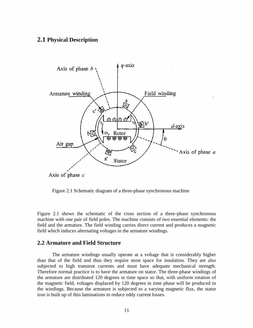
2.1 Physical Description

Figure 2.1 Schematic diagram of a three-phase synchronous machine

Figure 2.1 shows the schematic of the cross section of a three-phase synchronous

machine with one pair of field poles. The machine consists of two essential elements: the

field and the armature. The field winding carries direct current and produces a magnetic

field which induces alternating voltages in the armature windings.

2.2 Armature and Field Structure

The armature windings usually operate at a voltage that is considerably higher

than that of the field and thus they require most space for insulation. They are also

subjected to high transient currents and must have adequate mechanical strength.

Therefore normal practice is to have the armature on stator. The three-phase windings of

the armature are distributed 120 degrees in time space so that, with uniform rotation of

the magnetic field, voltages displaced by 120 degrees in time phase will be produced in

the windings. Because the armature is subjected to a varying magnetic flux, the stator

iron is built up of thin laminations to reduce eddy current losses.

12

When carrying balanced three-phase currents, the armature will produce a

magnetic field in the air gap rotating at synchronous speed. The field produced by the

direct current in the rotor winding on the other hand, revolves with the rotor. For

production of a steady torque, the fields of stator and rotor must rotate at the same speed.

Therefore, the rotor must run at precisely the synchronous speed.

The number of field poles is determined by the mechanical speed of the rotor and

electric frequency of stator currents. The synchronous speed is given by,

n = (120 f )/ pf - (1.1)

where n is the speed in rev/min, f is the frequency in Hz, and pf is the number of field

poles.

13

Chapter 3

Mathematical Description

of Synchronous Machine

14

3.1 Assumptions for developing the equations for synchronous machine

In developing equations of a synchronous machine, the following assumptions are

made:

(a) The stator windings are sinusoidally distributes along the air-gap as far as the

mutual effects with the rotor are concerned.

(b) The stator slots cause no appreciable variation of the rotor inductances with

rotor position.

(c) Magnetic hysteresis is negligible.

(d) Magnetic saturation effects are negligible.

Assumptions (a), (b), and (c) are reasonable. The principal justification comes from

the comparison of calculated performance. Assumption (d) is made for convenience

in analysis. With magnetic saturation neglected, we are required to deal with only

linear coupled circuits, making superposition applicable. However, saturation effects

are important.

Figure 3.1 shows the circuits involved in the analysis of a synchronous machine. The

stator circuits involved in the analysis of a synchronous machine. The rotor circuits

comprise field and amortisseur windings. The field winding is connected to a source

of direct current. For purpose of analysis, the currents in the amortisseur (solid rotor

and/or damper winding) may be assumed to flow in the two sets of closed circuits:

one set whose flux is in line with that of the field along the d-axis and the other set

whose flux is at right angles to the field axis or along the q-axis. The amortisseur

circuits take different forms and distinct, electrically independent circuits may not

exist. In Figure 3.1, only one amortisseur circuit is assumed in each axis.

15

a, b,c : Stator phase windings

fd: Field winding

kd : d-axis amortisseur circuit

kq : q-axis amortisseur circuit

k : 1,2,… n; n= no. of amortisseur circuits

θ : Angle by which d-axis leads the magnetic axis of phase a winding

wr: Rotor angular velocity, electrical rad/s

Figure 3.1 Stator and rotor circuits of a synchronous machine

In figure 3.1, θ is defined as the angle by which the d-axis leads the centerline of

phase a winding in the direction of rotation. Since the rotor is rotating with respect to the

stator, angle θ is continuously increasing and is related to the rotor angular velocity wr and

time t as follows:

θ = wr t - (3.1)

The electrical performance equations of a synchronous machine can be developed by

writing equations of the coupled circuits identified in Figure 3.1

16

3.2 Basic equations of a synchronous machine

The equations for the synchronous machine is developed using the generator

convention for polarities so that the positive direction of a stator winding current is

assumed to be out of the machine. The positive direction of field and amortisseur currents

is assumed to be into the machine.

In addition to the large number of circuits involved, the fact that the mutual and

self inductances of the stator circuits vary with rotor positions complicates the

synchronous machine equations. The variations in inductances are caused by the

variations in the permeances of the magnetic flux path due to non-uniform air-gap. This

is pronounced in a salient pole machine in which permances in the two axes are

significantly different. Even in a round rotor machine there are differences in the two

axes due mostly to the large number of slots associated with the field winding.

The flux produced by a stator by a stator winding follows a path through the stator

iron, across the air-gap, through the rotor iron, and back across the air-gap. The variations

in permeance of this path as a function of the rotor position can be approximated as,

- (3.2)

In the above equation, alpha is the angular distance from the d-axis along the periphery as

shown in figure 3.2.

Figure 3.2 Variation of permeance with rotor position

A double frequency variation is used produced, since the permeances of the north and

south poles are equal. Higher order even harmonics of permeance exist but are small

enough to be neglected.

17

We will use the following notations in writing the equations for the stator and rotor

circuits:

ea, eb ,ec = instantaneous stator phase to neutral voltages

ia, ib ,ic = instantaneous stator currents in phase a,b,c

ifd, ikd ,ikq = field and amortisseur currents

Rfd, Rkd ,Rkq = rotor circuit resistances

laa, lbb ,lcc = self inductance of stator windings

lab, lbc ,lca = mutual inductances between stator windings

lafd, lakd ,lakq = mutual inductances between stator and rotor windings

lffd, lkkd ,lkkq = self inductance of rotor windings

Ra = armature resistance per phase

p = differential operator d/dt

efd = field voltage

3.3 Stator Circuit Equations:

The voltage equations of the three phases are-

ea = (dΨa / dt) – ia Ra = pΨa – ia Ra …(3.3)

eb = pΨb – ib Ra …(3.4)

ec = pΨc – ic Ra …(3.5)

The flux linkage in the phase a winding at any instant is given by-

Ψa = -laa ia – lab ib –lac ifd + lakd ikd + lakq ikq …(3.6)

Similar expressions apply to flux linkages of windings b and c. The units used are

webers, henrys and amperes. The negative sign associated with the stator wonding

currents is due to their assumed direction.

3.4 Stator Self-inductances:

The self-inductance laa is equal to the ratio of flux linking phase a winding to the

current ia, with currents in all other circuits equal to zero. The inductance is directly

proportional to the permeance, which as indicated earlier has a second harmonic

variation. The inductance laa will be a maximum for θ = 0 degree, a minimum for θ = 90

degrees, a maximum again for θ= 180 degrees and so on.

Neglecting space harmonics, the mmf of phase a has a sinusoidal distribution in

space with its peak centred on the phase a axis. The peak amplitude of the mmf wave is

equal to Naia, where Na is the effective turns per phase. As shown in figure 3.3, this can

be resolved into two other sinusoidally distributed mmf‟s, one centred on the d-axis and

other on the q-axis.

18

The peak values of the two component waves are-

peak MMFad = Na ia cosθ …(3.7)

peak MMFaq = Na ia cos(θ+90) = -Na ia sinθ …(3.8)

The reason for resolving the mmf into the d-axis and q-axis components is that each acts

on specific air-gap geometry of defined configurations. Air-gap per pole along the two

axes are-

Фgad = (Na ia cosθ) Pd …(3.9)

Фgaq = (-Na ia sinθ) Pq …(3.10)

Figure 3.3 Phase a mmf wave and its components

The self inductance lga of phase a due to air-gap flux is-

lgaa = (Na фgoa)/ia

= Na2 { (Pd+Pq)/2 + (Pd-Pq)/2 cos2θ}

= Lg0 + Laa2cos2θ …(3.11)

The total self-inductance laa is given by adding to the above the leakage inductance Lal

which represents the leakage flux not crossing the air-gap:

laa = Lal + Lgaa

= Lal + Lg0 + Laa2 cos2θ

= Laa0 + Laa2 cos2θ …(3.12)

Since the windings of phases b and c are identical to that of phase a and are displaced

from it by 120 degrees and 240 degrees respectively, we have

lbb = Laa0 + Laa2 cos2(θ-120)

lcc = Laa0 + Laa2 cos2(θ+120) ...(3.13)

19

3.5 Stator Mutual Inductance:

The mutual inductances between any two stator windings also exhibits a second

harmonic variation because of the rotor shape. It is always negative, and has the greatest

absolute value when the north and south poles are equidistant from the centres of the two

windings concerned. For example, lab has maximium absolute value when θ = -30

degrees or θ = 150 degrees.

Thus the mutual inductances phase a and b, b and c, c and a are given as:

Lab = Lba = -Lab0 + Lab2 cos(2θ-120) …(3.14)

= -Lab0 - Lab2 cos(2θ+120)

Lbc = Lcb = -Lab0 - Lab2 cos(2θ+120) …(3.15)

Lca = Lac = -Lab0 - Lab2 cos(2θ+120) …(3.16)

The variation of mutual inductance between phases a and b as a function of θ is

illustrated in figure 3.4.

Figure 3.4 Variation of mutual inductance between stator windings

3.6 Mutual inductance between stator and rotor windings:

With the variations in air-gap due to stator slots neglected, the rotor circuits see a

constant permeance. Therefore, the situation in this case is not one of variation of

permeance; instead, the variation in the mutual inductance is due to the relative motion

between the windings themselves.When a stator winding is lined up with a rotor winding,

the flux linking the two windings is maximum and the mutual inductance is maximum.

When the two windings are displaced by 90 degrees, no flux links the two circuits and the

mutual inductance is zero.

20

With the sinusoidal distribution of mmf and flux waves,

lafd = Lafd cosθ

lakd = Lakd cosθ …(3.17)

lakq = Lakq cos(θ+90)

= -Lakq sinθ

For considering the mutual inductance between phase b winding and the rotor circuits, θ

is replaced by θ-120; for phase c winding θ is replaced by (θ+120).

Using the expressions for all the inductances that appear in stator voltage equations, we

have:

Ψa = - ia [ Laa0 + Laa2 cos2θ] + ib [ Lab0 + Laa2 cos(2θ+60)

+ ic [ Lab0 + Laa2 cos(2θ-30)] + ifd Lafd Cosθ …(3.18)

+ ikd Lakd cosθ – ikq Lakq sinθ

Similarly,

Ψb = - ia [ Lab0 + Laa2 cos(2θ+60)] - ib [ Laa0 + Laa2 cos2(θ-120)

+ ic [ Lab0 + Laa2 cos(2θ-180)] + ifd Lafd Cos(θ-120) …(3.19)

+ ikd Lakd cos(θ-120) – ikq Lakq sin(θ-120)

and

Ψc = - ia [ Lab0 + Laa2 cos(2θ-60)] + ib [ Lab0 + Laa2 cos2(θ-180) …(3.20)

- ic [ Laa0 + Laa2 cos2(θ+120)] + ifd Lafd Cos(θ+120)

+ ikd Lakd cos(θ+120) – ikq Lakq sin(θ+120)

3.7 Rotor circuit equations:

The rotor circuit voltage equations are:

efd = pΨfd + Rfd ifd …(3.21)

0 = pΨkd + Rkd ikd …(3.22)

0 = pΨkq + Rkq ikq …(3.23)

The rotor circuit flux linkages may be expresses as follows:

Ψfd = Lffd ifd + Lfkd ikd – Lafd [ iacosθ + ibcos(θ-120) + iccos(θ+120)]

Ψkd = Lfkd ifd + Lkkd ikd – Lakd [ iacosθ + ibcos(θ-120) + iccos(θ+120)] …(3.24)

Ψfq = Lkkq ikq + Lakq[ iasinθ + ibsin(θ-120) + iccos(θ+120)]

The rotor circuits see constant permeance because of the cylindrical structure of the

stator. Therefore, the self-inductances of rotor circuits and mutual inductances between

each other do not vary with rotor positions. Only the rotor to stator mutual inductances

vary periodically with θ.

21

Chapter 4

The dq0 Transformation

22

4.1 The dq0 Transformation:

The transformation from the abc phase variables to the dq0 variables can be

written in the following matrix form:

The inverse transformation is given by:

4.2 Stator flux linkages in dq0 components:

Transforming the flux linkages and currents into dq0 components and with

suitable reduction of terms involving trigonometric terms, we obtain the following

expressions:

..(4.1)

..(4.2) ..(4.3)

Defining the following new inductances:

..(4.4)

..(4.5) ..(4.6)

23

The flux linkage equation become

..(4.7)

..(4.8) ..(4.9)

The dq0 components of stator flux linkages are seen to be related to the components of

stator and rotor currents through constant inductances.

4.3 Rotor flux linkages in dq0 components:

..(4.10)

..(4.11)

..(4.12)

Again, all inductances are seen to be constant.

4.4 Stator voltage equations in dq0 components:

By applying dq0 transformation, following stator voltage equations are obtained:

..(4.13)

..(4.14)

..(4.15)

The angle θ is the angle between axis of phase a and d-axis. The term (p θ) in the above

equations represents angular velocity of the rotor.

4.5 Advantages of dq0 transformation:

The dq0 transformation may be viewed as a means of referring the stator

quantities to the rotor side.

The analysis of synchronous machine equations in terms of dq0 variables

considerably simpler than in terms of phase quantities for the following reasons:

The dynamic performance equations have constant inductances.

For balanced conditions, zero sequence quantities disappear.

For balanced steady-state operation, the stator quantities have constant values.

The parameters associated with d- and q-axis may be directly measured from terminal

tests.

24

4.6 Per unit representation:

In power system analysis, it is usually convenient to use a per unit system to

normalize system variables.

In the case of a synchronous machine, the per-unit system may be used to remove

arbitrary constants and simplify mathematical equations so that they may be expressed in

terms of equivalent circuits.

Per unit stator voltage equations:

..(4.16)

Per unit rotor voltage equations:

..(4.17)

For power system stability analysis, the machine equations are normally solved with all

quantities expressed in per unit.

25

Chapter 5

Operational parameters of

Synchronous machine

26

5.1 Synchronous Machine Parameters:

The synchronous machine equations developed in Chapter 3 have the inductances

and resistances of the stator and rotor circuits as parameters. These are referred to as

fundamental or basic parameters and are identified by the elements of the d- and q-axis

equivalent circuits. While the fundamental parameters completely specify the machine

electrical characteristics, they cannot be directly determined from the measured responses

of the machine. Therefore, the traditional approach to assigning machine data has been to

express them in terms of derived parameters that are related to observed behaviour as

viewed from the terminals under suitable test conditions.

5.2 Operational Parameters:

A convenient method of identifying the machine electrical characteristics is in

terms of operational parameters relating the armature and field terminal quantities.

Referring to Figure 4.1, the relationship between the incremental values of terminal

quantities may be expressed in the operational form as follows:

…(5.1)

…(5.2)

Figure 5.1 The d- and q-axis networks identifying terminals quantities

where,

G(s) is the stator to field transfer function

Ld(s) is the d-axis operational inductance

Lq(s) is the q-axis operational inductance

Equations 5.1 and 5.2 are true for any number of rotor circuits. With the equations in

operational form, the rotor can be considered as a distributed parameter system. The

operational parameters can be determined either from design calculations or more readily

from frequency response measurements.

27

When a finite number of rotor circuits are assumed, the operational parameters can be

expressed as a ratio of polynomial in s. The orders of the numerator and denominator

polynomials of Ld(s) and Lq(s) are equal to the number of rotor circuits assumed in the

respective axes, and G(s) has the same denominator as Ld(s), but a different numerator of

order one less than the denominator..

We will develop here the expressions for the operational parameters of the model

represented by the equivalent circuits shown in Figure 5.1. This model structure is

generally considered adequate for stability studies and is widely used in large scale

stability programs. The rotor characterstics are represented by the field winding and a

damper winding in the d-axis and the two damper windings in the q-axis. The mutual

inductances Lfd and Lad are assumed to be equal; this makes all mutual inductances in

the d-axis equal.

Figure 5.1 Structure of commonly used model

With equal mutual inductances, flux linkages for the d-axis in the operational

form can be written as:

The operational forms for rotor voltages are:

… 5.3

… 5.4

… 5.5

… 5.6

… 5.7

28

Our objective is to express the d-axis equations in the form of equations 5.1 and this can

be achieved by eliminating the rotor currents in terms of the terminal quantities efd and id.

Accordingly the solution of above two equations gives:

Where

Given that

… 5.8

… 5.9

… 5.10

… 5.11

… 5.12

29

substitution of equations 5.10 and 5.11 in the incremental form of equation 5.3 then gives

the relationship between d-axis quantities in the desired form:

The expressions for the d-axis operational parameters are given by:

where,

Equations 5.13 and 5.14 can be expressed in the factored form:

… 5.13

…5.14

… 5.5

… 5.15

… 5.16

… 5.17

30

The expression for the q-axis operational inductance may be written by inspection and

recognizing the similarities between d- and q- axis equivalent circuits. In the factored

form, it is given by:

The time constants associated with the expressions for Ld(s), Lq(s) and G(s) in the

factored form represent important machine parameters.

… 5.18

31

Chapter 6

Models of Synchronous

machine

32

6.1 Different Models of synchronous machines:

Depending upon the number of rotor windings on d-axis and q-axis and degree of

complexity following models are suggested:

1. Classical model ( Model 0.0)

2. Field circuit only (Model 1.0)

3. Field circuit with one equivalent damper on q-axis (Model 1.1)

4. Field circuit with one equivalent damper on d-axis –

(a) Model 2.1 (one damper on q-axis)

(b) Model 2.2 (two damper on q-axis)

5. Field circuit with two equivalent damper circuits on d-axis –

(a) Model 3.2 (with two damper on q-axis)

(b) Model 3.3 (with three dampers on q-axis)

It is to be noted that in the classification of the machine models, the first number

indicates the number of winding on the d-axis while the second number indicates the

number of windings on the q axis.(Alternatively the number represent the number of state

variables considered in the d axis and q axis).Thus, the classical model which neglects

damper winding circuits and field flux decay, ignores all sate variable for the rotor coil

and is termed (0.0)

6.2 Applications of different models:

Model (2.2) is widely used in the literature. Model (3.3) is claimed to be the most

detailed model applicable to turbogenerator, while models (2.1) and (1.1) are widely used

for hydro generators. It is to be noted that while higher order models provide better

result for such applications, they also require an exact determination of parameters.

With constraints on data availability and for study of large systems, it may be adequate to

use model (1.1) if the data is correctly determined.

33

In the project, Model (0.0), Model(2.1) and Model(2.2) have been analysed

mathematically and simulated to obtain machine‟s fundamental parameters.

34

Chapter 7

Analysis of Models for

Synchronous machine

35

7.1 Model (2.1) :

The standard representation of a Synchronous machine is done by using

Model(2.1) which includes field circuit and an equivalent damper winding on d-axis and

a damper winding on q-axis.

Following assumptions are being made during analysis of the model :

Main field flux decay is considered.

An equivalent damper winding included in both q – axis and d-axis each.

Speed is assumed to be constant.

Saturation is neglected.

7.1.1 Equivalent circuits

Equivalent circuits representing the complete characteristics of the synchronous

machines for direct axis and qudrature axis is shown in Fig-1 and Fig-2 respectively

below-

Fig-7.1 d-axis and q-axis equivalent circuits for model (2.1)

In the d-axis equivalent circuit, there is a field winding and a damper winding along with

a field source. In the case of q-axis, there is no field winding and the amortisseurs

represent the overall effect of the damper windings and eddy current paths.

36

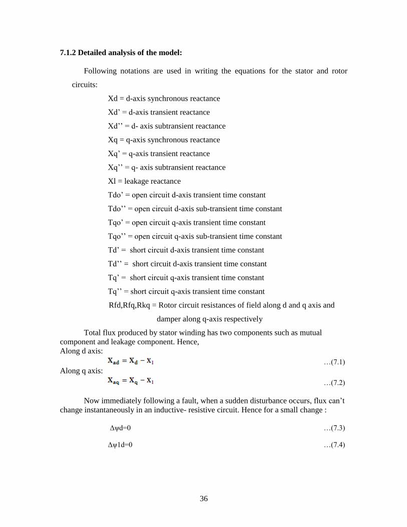
7.1.2 Detailed analysis of the model:

Following notations are used in writing the equations for the stator and rotor

circuits:

Xd = d-axis synchronous reactance

Xd‟ = d-axis transient reactance

Xd‟‟ = d- axis subtransient reactance

Xq = q-axis synchronous reactance

Xq‟ = q-axis transient reactance

Xq‟‟ = q- axis subtransient reactance

Xl = leakage reactance

Tdo‟ = open circuit d-axis transient time constant

Tdo‟‟ = open circuit d-axis sub-transient time constant

Tqo‟ = open circuit q-axis transient time constant

Tqo‟‟ = open circuit q-axis sub-transient time constant

Td‟ = short circuit d-axis transient time constant

Td‟‟ = short circuit d-axis transient time constant

Tq‟ = short circuit q-axis transient time constant

Tq‟‟ = short circuit q-axis transient time constant

Rfd,Rfq,Rkq = Rotor circuit resistances of field along d and q axis and

damper along q-axis respectively

Total flux produced by stator winding has two components such as mutual

component and leakage component. Hence,

Along d axis:

…(7.1)

Along q axis:

…(7.2)

Now immediately following a fault, when a sudden disturbance occurs, flux can‟t

change instantaneously in an inductive- resistive circuit. Hence for a small change :

Δψd=0 …(7.3)

Δψ1d=0 …(7.4)

37

Thus equivalent circuit is reduced to a open circuit consisting of three parallel branches

and corresponding equation for d-axis is:

…(7.5)

Similarly for q axis equivalent equation can be written as –

…(7.6)

7.1.3 Derivation for obtaining open circuit time constants:

The relationship of open circuit time constants can be found by open circuiting

the AB branch of the circuit (from fig. shown below). During open circuit condition,

current through this branch is zero.

Thus, admittance = Δid(s)/Δed(s) = 0

Figure 7.2d-axis and q-axis equivalent circuits for model (2.1)

to obtain open circuit time constants

Thus the equations for transient and sub-transient case along d-axis and q-axis are:

…(7.7)

…(7.8)

38

…(7.9)

..(7.10)

7.1.4 Derivation for Short circuit time constants :

Equivalent circuit diagram is short circuited to obtain the relations .Here only

additional term Xl will be introduced which is obvious from the figure shown below:

Figure 7.3 d-axis equivalent circuit for model (2.1)

to obtain short circuit time constants

The equations for transient and sub-transient conditions for short circuit situation along d-

axis and q-axis are:

..(7.11)

..(7.12)

..(7.13)

..(7.14)

Now from operational analysis of inductance ,we know that-

..(7.15)

39

For sub-transient condition, when „s‟tends to zero, sub-transient reactance along d-axis is

obtained as:

..(7.16)

Similarly, Transient reactance along d-axis is obtained as

..(7.17)

Thus ..(7.18)

Similarly following relation can be obtained:

..(7.19)

To find the parameters involved in the equations Newton- raphson method has been

applied where initial values are taken considering following equations-

..(7.20)

..(7.21)

..(7.22)

..(7.23)

..(7.24)

..(7.25)

..(7.26)

..(7.27)

..(7.28)

..(7.29)

..(7.30)

40

..(7.31)

..(7.32)

..(7.33)

These equations are being solved using NEWTON RAPHSON method and simulated in

MATLAB using a set of manufacturer‟s data, taken from an IEEE Transaction on Power

Apparatus and Systems, Vol. PAS-96, no.5. “First benchmark model for computer

simulation of sub synchronous resonance.”

7.1.5 Simulation Result:

The equations were simulated using manufacturer‟s data given in Table 6.1 and

fundamental parameters were obtained shown in Table 6.2

Table 7.1 Manufacturer provided data

Table 7.2 d-axis and q-axis parameters for model(2.1)

Xa

d

(pu

)

Xa

q

(pu

)

Xfd

(pu)

Xfq

(pu)

Xkd

(pu)

X1q

(pu)

Rfd

(pu)

Rfq

(pu

)

Rkd

(pu)

R1

q

(pu

)

Td‟

(s)

Td‟‟

(s)

Tq‟

(s)

Tq‟‟

(s)

1.6

6

1.5

8

0.039

9

0.104

5

0.005

7

0.245

0

0.395

3

1.9

8

1.39

8

6.8

6

0.406

0

0.025

6

0.113

3

0.043

9

Xd

(pu)

Xq

(pu)

Xd‟

(pu)

Xq‟

(pu)

Xd‟‟

(pu)

Xq‟‟

(pu)

Tdo‟

(s)

Tqo‟

(s)

Tdo”

(s)

Tqo”

(s)

Xl

(pu)

1.79 1.71 0.169 0.228 0.135 0.2 4.3 0.85 0.032 0.05 0.13

41

7.2 Model(0.0):

This is the simplest model of the machine representation, also called as “Classical

Model”. The model has only field circuit on d-axis with no damper windings on either

axis.

Following are the assumptions used during mathematical analysis of the model:

Transformer voltages in the stator equations are neglected

Speed is assumed constant

Effect damper windings are neglected

Saturation is not simulated

Main flux linkages are assumed to be constant

Transient saliency is neglected, that is approximating

7.2.1 Equivalent circuit:

The circuit diagram for model (0.0) is obtained from the flux model analysis and the

circuit is shown below for both d-axis and q-axis axis:


42

7.2.2: Circuit Equations:

Following equations can be derived from equivalent circuits using flux model

analysis as done for model (2.1) :

..(7.34)

..(7.35)

..(7.36)

..(7.37)

..(7.38)

..(7.39)

..(7.40)

..(7.41)

..(7.42)

..(7.43)


Above equations were simulated using the same machine data provided by

manufacturer for model(2.1) and following results were obtained as shown in Table 6.3:


Xad

(pu)

Xaq

(pu)

Xfd

(pu)

Xfq

(pu)

Rfd

(pu)

Rfq

(pu)

Td‟

(s)

Td‟‟

(s)

Tq‟

(s)

Tq‟‟

(s)

1.66 1.58 0.0399 0.1045 0.3953 1.9817 0.4060 0.0256 0.1133 0.0439

43

7.3 Model (2.2):

This is a representation intended to maintain a balance by using two windings

(one field, one equivalent damper)on d-axis and two equivalent dampers on q-axis.

Following assumptions have been used for analysis of the model:

Main field flux decay is considered.

Two equivalent damper winding included in q – axis.

One equivalent damper winding included in d– axis.

Speed is assumed constant.

Saturation is neglected.

7.3.1 Equivalent circuit:

The circuit diagram for both d-axis and q- axis has been shown below :


44

7.3.2 Circuit Equations:

As developed in previous models the relationship between various time constants

and transient parameter can be found out from equivalent circuits. The circuit equations

are shown below:

..(7.44)

..(7.45)

..(7.46)

..(7.47)

..(7.48)

..(7.49)

..(7.50)

..(7.51)

..(7.52)

..(7.53)

..(7.54)

..(7.55)

..(7.56)

45

..(7.57)

..(7.58)

..(7.59)


The above equations were simulated using NEWTON RAPHSON method in

MATLAB using the same machine data provided by manufacturer as done for previous

models .Following fundamental parameters were obtained as shown in Table 6.4:


Xad

(pu)

Xaq

(pu)

Xfd

(pu)

Xfq

(pu)

Xkd

(pu)

X1q

(pu)

X2q

(pu)

Rfd

(pu)

Rfq

(pu)

Rkd

(pu)

R1q

(pu)

R2q

(pu)

1.66 1.58 0.0399 0.1045 0.0057 0.1045 0.2450 0.3953 1.9817 1.3980 3.4896 5.9114

Td‟

(s)

Td‟‟

(s)

Tq‟

(s)

Tq‟‟

(s)

0.4060 0.0256 0.1133 0.0439

46

Chapter 8

MATLAB Simulation for

the Synchronous machine

Models

47

8.1 MAIN FILE

% MAIN FILE clear all; close all; clc B=zeros(10,1); J=zeros(10,10); I=zeros(10,10); resm=zeros(10,6); resm1=zeros(10,6); resd=zeros(10,6); resd1=zeros(10,6); disp('BTECH FINAL YEAR PROJECT') disp('========================') disp('Enter intial values :PARA METERS IN DATASHEET ') % y1=input('Xd : '); % y2=input('Xq : '); % y3=input('Xd1 : '); % y4=input('Xq1 : '); % y5=input('Xd2 : '); % y6=input('Xq2 : '); % y7=input('Tdo1 : '); % y8=input('Tqo1 : '); % y9=input('Tdo2 : '); % y10=input('Tqo2 : '); % y11=input('Xl :'); y1=1.79; y2=1.71; y3=0.169; y4=0.228; y5=0.135; y6=0.2; y7=4.3; y8=0.85; y9=0.032; y10=0.05; y11=0.13; disp('=====================================================================') disp('FOR MODEL1 ....NO DAMPER ATALL... ') disp('=====================================================================') disp('=====================================================================') disp('INITIALIZATION OF PARAMETERS TO B ESTIMATED..ENTER INITIAL VALUE... ') disp('=====================================================================') % x1=input('Xad : '); % x2=input('Xaq : '); % x3=input('Xfd : '); % x4=input('Xfq : '); % x5=input('Xkd : '); % x6=input('Xkq : ');

48

% x7=input('Rfd : '); % x8=input('Rfq : '); % x9=input('Rkd : '); % x10=input('Rkq : '); % x11=input('Td1 : '); % x12=input('Td2 : '); % x13=input('Tq1 : '); % x14=input('Tq2 : '); x1=1; x2=1; x3=0.01; x4=0.1; x5=0.001; x6=0.1; x7=0.001; x8=0.001; x9=0.001; x10=0.01; x11=0.01; x12=0.01; x13=0.1; x14=0.01; k=1; DX =ones(14,1); ecc=0.0001; disp('=====================WAIT ITERATION GOING ON================') for a=1:1:10 k=k+1; for i=1:1:10 d=1;j=1; B(i)=0- lfun1(x1,x2,x3,x4,x7,x8,x11,x12,x13,x14,y1,y2,y3,y4,y5,y6,y7,y8,y9,y10,y11,i,j,d); j=2; for d=1:1:10 J(i,d)=lfun1(x1,x2,x3,x4,x7,x8,x11,x12,x13,x14,y1,y2,y3,y4,y5,y6,y7,y8,y9,y10,y11,i,j,d); end end det(J); I=inv(J); DX=I*B; disp(a) %Updation of variables x1= x1+DX(1); x2= x2+DX(2); x3= x3+DX(3); x4= x4+DX(4); x7= x7+DX(5); x8= x8+DX(6); x11= x11+DX(7); x12= x12+DX(8); x13= x13+DX(9);x14= x14+DX(10); resd(a,1)=a; resd1(a,1)=a; resd(a,2)=DX(1); resd(a,3)=DX(2); resd(a,4)=DX(3); resd(a,5)=DX(4); resd(a,6)=DX(5); resd1(a,2)=DX(6); resd1(a,3)=DX(7); resd1(a,4)=DX(8); resd1(a,5)=DX(9); resd1(a,6)=DX(10); m1=x1;m2=x2;m3=x3;m4=x4;m7=x7; m8=x8; m11=x11;m12=x12;m13=x13;m14=x14;

49

resm(a,1)=a; resm(a,2)=m1; resm(a,3)=m2;resm(a,4)=m3; resm(a,5)=m4; resm(a,6)=m7*377; resm1(a,1)=a; resm1(a,2)=m8*377;resm1(a,3)=m11; resm1(a,4)=m12;resm1(a,5)=m13;resm1(a,6)=m14; end disp('ESTIMATED PARAMETERS AND RESIDUAL VALUES ARE') disp('=============================================') disp(' ITERNO Xad Xaq Xfd Xfq Rfd '); disp(' ====== === === === === === '); disp(resm); disp(' ITERNO Rfq Td1 Td2 Tq1 Tq2 '); disp(' ====== === === === === === '); disp(resm1); disp('=====================================================================') disp(' RESIDUE MATRIX'); disp('=====================================================================') disp(' ITERNO Xad Xaq Xfd Xfq Rfd '); disp(' ====== === === === === === '); disp(resd); disp(' ITERNO Rfq Td1 Td2 Tq1 Tq2 '); disp(' ====== === === === === === '); disp(resd1); disp('========================================================================') disp('=====================================================================') disp('FOR MODEL2 ....1 DAMPER IN D AXIS AND 1 IN Q AXIS... ') disp('=====================================================================') disp('=====================================================================') disp('INITIALIZATION OF PARAMETERS TO B ESTIMATED..ENTER INITIAL VALUE... ') disp('=====================================================================') B=zeros(14,1); J=zeros(14,14); I=zeros(14,14); resm=zeros(10,8); resm1=zeros(10,8); resd=zeros(10,8); resd1=zeros(10,8); k=1; DX =ones(14,1); ecc=0.0001; disp('=====================WAIT ITERATION GOING ON================') for a=1:1:10 k=k+1; for i=1:1:14 d=1;j=1; B(i)=0-lfun2(x1,x2,x3,x4,x5,x6,x7,x8,x9,x10,x11,x12,x13,x14,y1,y2,y3,y4,y5,y6,y7,y8,y9,y10,y11,i,j,d); j=2;

50

for d=1:1:14 J(i,d)=lfun2(x1,x2,x3,x4,x5,x6,x7,x8,x9,x10,x11,x12,x13,x14,y1,y2,y3,y4,y5,y6,y7,y8,y9,y10,y11,i,j,d); end end det(J); I=inv(J); DX=I*B; disp(a) %Updation of variables x1= x1+DX(1); x2= x2+DX(2); x3= x3+DX(3); x4= x4+DX(4); x5= x5+DX(5); x6= x6+DX(6); x7= x7+DX(7); x8= x8+DX(8); x9= x9+DX(9); x10= x10+DX(10); x11= x11+DX(11); x12= x12+DX(12); x13= x13+DX(13); x14= x14+DX(14); resd(a,1)=a; resd1(a,1)=a; resd(a,2)=DX(1); resd(a,3)=DX(2); resd(a,4)=DX(3); resd(a,5)=DX(4); resd(a,6)=DX(5); resd(a,7)=DX(6); resd(a,8)=DX(7); resd1(a,2)=DX(8); resd1(a,3)=DX(9); resd1(a,4)=DX(10); resd1(a,5)=DX(11); resd1(a,6)=DX(12); resd1(a,7)=DX(13); resd1(a,8)=DX(14); m1=x1; m2=x2; m3=x3; m4=x4; m5=x5; m6=x6; m7=x7; m8=x8; m9=x9; m10=x10; m11=x11; m12=x12; m13=x13; m14=x14; resm(a,1)=a; resm(a,2)=m1; resm(a,3)=m2; resm(a,4)=m3; resm(a,5)=m4; resm(a,6)=m5; resm(a,7)=m6; resm(a,8)=m7*377; resm1(a,1)=a; resm1(a,2)=m8*377; resm1(a,3)=m9*377; resm1(a,4)=m10*377; resm1(a,5)=m11; resm1(a,6)=m12; resm1(a,7)=m13; resm1(a,8)=m14; end

51

disp('ESTIMATED PARAMETERS AND RESIDUAL VALUES ARE') disp('=============================================') disp(' ITERNO Xad Xaq Xfd Xfq Xkd Xkq Rfd '); disp(' ====== === === === === === === === '); disp(resm); disp(' ITERNO Rfq Rkd Rkq Td1 Td2 Tq1 Tq2 '); disp(' ====== === === === === === === === '); disp(resm1); disp('========================================================================================') disp(' RESIDUE MATRIX'); disp('========================================================================================') disp(' ITERNO Xad Xaq DXfd Xfq Xkd Xkq Rfd '); disp(' ====== === === === === === === === '); disp(resd); disp(' ITERNO Rfq Rkd Rkq Td1 Td2 Tq1 Tq2 '); disp(' ====== === === === === === === === '); disp(resd1); disp('=====================================================================') disp('FOR MODEL3 ....1 DAMPER IN D AXIS AND 2 IN Q AXIS... ') disp('=====================================================================') disp('=====================================================================') disp('INITIALIZATION OF PARAMETERS TO B ESTIMATED..ENTER INITIAL VALUE... ') disp('=====================================================================') B=zeros(16,1); J=zeros(16,14); I=zeros(16,14); resm=zeros(7,9); resm1=zeros(7,9); resd=zeros(7,9); resd1=zeros(7,9); y1=1.79; y2=1.71; y3=0.169; y4=0.228; y5=0.135; y6=0.2; y7=4.3; y8=0.85; y9=0.032; y10=0.05; y11=0.13; x1=1; x2=1; x3=0.01; x4=0.1; x5=0.001; x6=0.2; x7=0.001; x8=0.001; x9=0.001;

52

x10=0.02; x11=0.01; x12=0.01; x13=0.1; x14=0.01; x15=0.2; x16=0.02; % x1=input('Xad : '); % x2=input('Xaq : '); % x3=input('Xfd : '); % x4=input('Xfq : '); % x5=input('Xkd : '); % x6=input('X1q : '); % x15=input('X2q : '); % x7=input('Rfd : '); % x8=input('Rfq : '); % x9=input('Rkd : '); % x10=input('R1q : '); % x16=input('R2q : '); % x11=input('Td1 : '); % x12=input('Td2 : '); % x13=input('Tq1 : '); % x14=input('Tq2 : '); k=1; DX =ones(16,1); ecc=0.0001; disp('=====================WAIT ITERATION GOING ON================') for a=1:1:7 k=k+1; for i=1:1:16 d=1;j=1; B(i)=0-lfun4(x1,x2,x3,x4,x5,x6,x7,x8,x9,x10,x11,x12,x13,x14,x15,x16,y1,y2,y3,y4,y5,y6,y7,y8,y9,y10,y11,i,j,d); j=2; for d=1:1:16 J(i,d)=lfun4(x1,x2,x3,x4,x5,x6,x7,x8,x9,x10,x11,x12,x13,x14,x15,x16,y1,y2,y3,y4,y5,y6,y7,y8,y9,y10,y11,i,j,d); end end det(J); I=inv(J); DX=I*B; disp(a) %Updation of variables x1= x1+DX(1); x2= x2+DX(2); x3= x3+DX(3); x4= x4+DX(4); x5= x5+DX(5); x6= x6+DX(6); x7= x7+DX(7); x8= x8+DX(8); x9= x9+DX(9);

53

x10= x10+DX(10); x11= x11+DX(11); x12= x12+DX(12); x13= x13+DX(13); x14= x14+DX(14); x15= x15+DX(15); x16= x16+DX(16); resd(a,1)=a; resd1(a,1)=a; resd(a,2)=DX(1); resd(a,3)=DX(2); resd(a,4)=DX(3); resd(a,5)=DX(4); resd(a,6)=DX(5); resd(a,7)=DX(6); resd(a,8)=DX(15); resd(a,9)=DX(7); resd1(a,2)=DX(8); resd1(a,3)=DX(9); resd1(a,4)=DX(10); resd1(a,5)=DX(16); resd1(a,6)=DX(11); resd1(a,7)=DX(12); resd1(a,8)=DX(13); resd1(a,9)=DX(14); m1=x1;m2=x2; m3=x3;m4=x4;m5=x5;m6=x6;m7=x7;m8=x8;m9=x9; m10=x10;m11=x11;m12=x12; m13=x13;m14=x14;m15=x15;m16=x16; resm(a,1)=a; resm(a,2)=m1; resm(a,3)=m2; resm(a,4)=m3; resm(a,5)=m4; resm(a,6)=m5; resm(a,7)=m6; resm(a,8)=m15; resm(a,9)=m7*377; resm1(a,1)=a; resm1(a,2)=m8*377; resm1(a,3)=m9*377; resm1(a,4)=m10*377; resm1(a,5)=m16*377; resm1(a,6)=m11; resm1(a,7)=m12; resm1(a,8)=m13; resm1(a,9)=m14; end disp('ESTIMATED PARAMETERS AND RESIDUAL VALUES ARE') disp('=============================================') disp(' ITERNO Xad Xaq Xfd Xfq Xkd X1q X2q Rfd '); disp(' ====== === === === === === === === ==== '); disp(resm); disp(' ITERNO Rfq Rkd R1q R2q Td1 Td2 Tq1 Tq2 '); disp(' ====== === === === === === === === === '); disp(resm1);

54

disp('========================================================================================') disp(' RESIDUE MATRIX'); disp('========================================================================================') disp(' ITERNO Xad Xaq Xfd Xfq Xkd X1q X2q Rfd '); disp(' ====== === === === === === === === ==== '); disp(resd); disp(' ITERNO Rfq Rkd R1q R2q Td1 Td2 Tq1 Tq2 '); disp(' ====== === === === === === === === === '); disp(resd1); disp('========================================================================================') disp(' ********THANKING YOU******** ') disp('========================================================================================')

55

FUNCTION CODE FOR MODEL(0.0) :

Function f1=lfun1(x1,x2,x3,x4,x7,x8,x11,x12,x13,x14,y1,y2,y3,y4,y5,y6,y7,y8,y9,y10,y11,i,j,d); syms z1; syms z2; syms z3; syms z4; syms z7; syms z8; syms z11; syms z12; syms z13; syms z14; if i==1 g=y1-y11-z1; end if i==2 g=y2-y11-z2; end if i==3 g=(1/(y3-y11))-(1/z1)-(1/z3); end if i==4 g=(1/(y4-y11))-(1/z2)-(1/z4); end if i==5 g=((z3+z1)/(377*y7)) -z7; end if i==6 g=((z4+z2)/(377*y8))-z8; end if i==7 g=(y3*y7)/y1 - z11; end if i==8 g=(y4*y8)/y2 - z13; end if i==9 g=(y5*y9)/y3 - z12; end if i==10

56

g=(y6*y10)/y4 - z14; end if(j==1) f2=subs(g,{z1,z2,z3,z4,z7,z8,z11,z12,z13,z14},{x1,x2,x3,x4,x7,x8,x11,x12,x13,x14}); f1=double(f2); end if(j==2) if d==1 der=diff(g,z1); end if d==2 der=diff(g,z2); end if d==3 der=diff(g,z3); end if d==4 der=diff(g,z4); end if d==5 der=diff(g,z7); end if d==6 der=diff(g,z8); end if d==7 der=diff(g,z11); end if d==8 der=diff(g,z12); end if d==9 der=diff(g,z13); end if d==10 der=diff(g,z14); end f2=subs(der,{z1,z2,z3,z4,z7,z8,z11,z12,z13,z14},{x1,x2,x3,x4,x7,x8,x11,x12,x13,x14}); f1=double(f2); end end

57

FUNCTION CODE FOR MODEL(2.1) :

function f1=lfun2(x1,x2,x3,x4,x5,x6,x7,x8,x9,x10,x11,x12,x13,x14,y1,y2,y3,y4,y5,y6,y7,y8,y9,y10,y11,i,j,d); syms z1; syms z2; syms z3; syms z4; syms z5; syms z6; syms z7; syms z8; syms z9; syms z10; syms z11; syms z12; syms z13; syms z14; if i==1 g=y1-y11-z1; end if i==2 g=y2-y11-z2; end if i==3 g=(1/(y3-y11))-(1/z1)-(1/z3); end if i==4 g=(1/(y4-y11))-(1/z2)-(1/z4); end if i==5 g=(1/(y5-y11))-(1/(y3-y11))-(1/z5); end if i==6 g=(1/(y6-y11))-(1/(y4-y11))-(1/z6); end if i==7 g=((z3+z1)/(377*y7)) -z7; end if i==8 g=((z4+z2)/(377*y8))-z8; end if i==9 g=((z5*z1 + z5*z3 + z1*z3)/((377*y9)*(z1+z3))) - z9; end if i==10 g=((z6*z2 + z6*z4 + z2*z4)/((377*y10)*(z2+z4))) - z10; end if i==11 g=(y3*y7)/y1 - z11; end if i==12 g=(y4*y8)/y2 - z13; end

58

if i==13 g=(y5*y9)/y3 - z12; end if i==14 g=(y6*y10)/y4 - z14; end if(j==1) f2=subs(g,{z1,z2,z3,z4,z5,z6,z7,z8,z9,z10,z11,z12,z13,z14},{x1,x2,x3,x4,x5,x6,x7,x8,x9,x10,x11,x12,x13,x14}); f1=double(f2); end if(j==2) if d==1 der=diff(g,z1); end if d==2 der=diff(g,z2); end if d==3 der=diff(g,z3); end if d==4 der=diff(g,z4); end if d==5 der=diff(g,z5); end if d==6 der=diff(g,z6); end if d==7 der=diff(g,z7); end if d==8 der=diff(g,z8); end if d==9 der=diff(g,z9); end if d==10 der=diff(g,z10); end if d==11 der=diff(g,z11); end if d==12 der=diff(g,z12); end if d==13 der=diff(g,z13); end if d==14 der=diff(g,z14);

59

end f2=subs(der,{z1,z2,z3,z4,z5,z6,z7,z8,z9,z10,z11,z12,z13,z14},{x1,x2,x3,x4,x5,x6,x7,x8,x9,x10,x11,x12,x13,x14}); f1=double(f2); end end

FUNCTION CODE FOR MODEL(2.2):

function f1=lfun4(x1,x2,x3,x4,x5,x6,x7,x8,x9,x10,x11,x12,x13,x14,x15,x16,y1,y2,y3,y4,y5,y6,y7,y8,y9,y10,y11,i,j,d); syms z1; syms z2; syms z3; syms z4; syms z5; syms z6; syms z7; syms z8; syms z9; syms z10; syms z11; syms z12; syms z13; syms z14; syms z15; syms z16; if i==1 g=y1-y11-z1; end if i==2 g=y2-y11-z2; end if i==3 g=(1/(y3-y11))-(1/z1)-(1/z3); end if i==4 g=(1/(y4-y11))-(1/z2)-(1/z4); end if i==5 g=(1/(y5-y11))-(1/(y3-y11))-(1/z5); end if i==6 g=y11+(1/((1/z2)+(1/z6)))-y4; % g=(1/(y6-y11))-(1/(y4-y11))-(1/z6)-(1/z15); end if i==7 g=((z3+z1)/(377*y7)) -z7; end if i==8 g=((z4+z2)/(377*y8))-z8; end if i==9

60

g=((z5*z1 + z5*z3 + z1*z3)/((377*y9)*(z1+z3))) - z9; end if i==10 g=(1/(377*y10))*(z6+(z15*z2*z4/(z15*z2+z15*z4+z2*z4)))-z10; end if i==11 g=(y3*y7)/y1 - z11; end if i==12 g=(y4*y8)/y2 - z13; end if i==13 g=(y5*y9)/y3 - z12; end if i==14 g=(y6*y10)/y4 - z14; end if i==15 g=y11+(1/((1/z2)+(1/z6)+(1/z15)))-y6; % g=y11+(1/((1/x2)+(1/x6)+(1/x15)+(1/x4)))-y5; end if i==16 g=((z15+(z6*z2*z4/(z6*z2+z6*z4+z2*z4)))/(377*y10))-z16; end if(j==1) f2=subs(g,{z1,z2,z3,z4,z5,z6,z7,z8,z9,z10,z11,z12,z13,z14,z15,z16},{x1,x2,x3,x4,x5,x6,x7,x8,x9,x10,x11,x12,x13,x14,x15,x16}); f1=double(f2); end if(j==2) if d==1 der=diff(g,z1); end if d==2 der=diff(g,z2); end if d==3 der=diff(g,z3); end if d==4 der=diff(g,z4); end if d==5 der=diff(g,z5); end if d==6 der=diff(g,z6); end if d==7 der=diff(g,z7); end if d==8 der=diff(g,z8);

61

end if d==9 der=diff(g,z9); end if d==10 der=diff(g,z10); end if d==11 der=diff(g,z11); end if d==12 der=diff(g,z12); end if d==13 der=diff(g,z13); end if d==14 der=diff(g,z14); end if d==15 der=diff(g,z15); end if d==16 der=diff(g,z16); end f2=subs(der,{z1,z2,z3,z4,z5,z6,z7,z8,z9,z10,z11,z12,z13,z14,z15,z16},{x1,x2,x3,x4,x5,x6,x7,x8,x9,x10,x11,x12,x13,x14,x15,x16}); f1=double(f2); end end

62

Chapter 9

Conclusion

63

10.1 A Comparative Study of Fundamental Parameters for different

Models of Synchronous Machine:

Table 10.1 Comparative chart for fundamental parameters of same synchronous machine represented by

three different models

`Sl. No.

Parameters Model(0.0) Model(2.1) Model(2.2)

1. Xad

1.66 1.66 1.66

2. Xaq

1.58 1.58 1.58

3. Xfd

0.0399 0.0399 0.0399

4. Xfq

0.1045 0.1045 0.1045

5.

Xkd - 0.0057 0.0057

6.

X1q - 0.2450 0.1045

7.

X2q - - 0.2450

8.

Rfd 0.3953 0.3953 0.3953

9.

Rfq 1.9817 1.9817 1.9817

10.

Rkd - 1.3980 1.3980

11.

R1q - 6.8600 3.4896

12.

R2q - - 5.9114

13.

Td1 0.4060 0.4060 0.4060

14.

Td2 0.0256 0.0256 0.0256

15.

Tq1 0.1133 0.1133 0.1133

16. Tq2 0.0439 0.0439 0.0439

64

10.2 Discussion: Stability analysis is one of the most important tasks in power system operations and

planning. Synchronous generators play a very important role in this way. A valid model

for synchronous generators is essential for a reliable analysis of stability and dynamic

performance. Almost three quarters of a century after the first publications in modeling

synchronous generators, this subject is still a challenging and attractive research topic.

Two axis equivalent circuits are commonly used to represent the behavior of synchronous

machines. The direct determination of circuit parameters from design data is very

difficult due to intricate geometry and nonlinear constituent parts of machines. So several

tests have been developed which indirectly obtain the parameter values of equivalent

circuits.

10.3 Comparison among different models:

Synchronous machine models of various degrees of complexity have been developed

from the fundamental parameters.The comparison of machine models is useful in the

evaluation of the transient performance of multimachine power systems. Synchronous-

machine models of various degrees of complexity which are developed from the

fundamental machine equations show different responses. They can be used to simulate

the transient behavior of a simple multimachine power system under both non-pole-

slipping and pole-slipping conditions. The comparisons made between predicted and

actual responses can show the degree of accuracy which may be expected for the various

models employed.

Model (2.2) is widely used in the literature. Model (3.3) is claimed to be the most

detailed model applicable to turbogenerator, while models (2.1) and (1.1) are widely used

for hydro generators. It is to be noted that while higher order models provide better result

for such applications, they also require an exact determination of parameters.With

constraints on data availability and for study of large systems, it may be adequate to use

model (1.1) if the data is correctly determined.

Models in which sub transient phenomena are simulated, but where some transformer

voltages in the stator equations, together with sub transient saliency, are neglected,

65

provide a model which is adequate and economical in computing demands for system

disturbances including those in which the machine may momentarily fall from

synchronism. Model (2.2) can fulfill these requirements in all but specialized studies of

an exacting nature, with certain simplification like Model (2.2) becomes more

economical in computational requirements.

66

REFERENCES

[1] Kundur Prabha,Power System Stability and Control, Tata McGraw-Hill Publishing

Company Limited,2007.

[2] Wadhwa, C.L., Electrical Power Systems, New Delhi, New Age International

publishers, 2005.

[3] IEEE Subsynchronous Resonance Task Force of the Dynamic System Performance

Working Group Power System Engineering Committee, “ First Benchmark Model For

Computer Simulation of Sunsynchronous Resonanace”,Vol. PAS-96, no. 5,

September/October 1977.

[4] Yao-nan Yu, H.A.M. Moussa, “Experimantal Details of Exact Equivalent Circuit

Parameters of Synchronous Machines”, IEEE Trans. On Power Apparatus and Systems,

Vol. PAS-90, Nov./ Dec. 1971.

[5] M.R.Aghamohammadi, M.Pourgholi, “ Experience with SSFR Test for

Synchronous Generator Model Identification Using Hook-Jeeves Optimization Method”,

international Journal of Systems Applications, Engineering & Development, Issue 3,

Volume2, 2008.

[6] Bernard Adkins, The General Theory of Electrical Machines, London, Chapman &

Hall Ltd., 1957, pp. 101-124, pp. 145-151.

[7] IEEE Standard Procedures for Obtaining Synchronous Machine Parameters by

Standstill Frequency Response Testing (Supplement to ANSI/IEEE Std 115-1983)

67

[8] H. Bora Karayaka, Ali Keyhani, Fellow, IEEE, Gerald Thomas Heydt, Fellow, IEEE,

Baj L. Agrawal, Fellow, IEEE, and Douglas A. Selin, Senior Member, IEEE,

“Synchronous Generator Model Identification and Parameter Estimation From

Operating Data”

[9] R.H.Park , “Two-Reaction Theory of Synchronous Machine”, NAPS, UNIVERSITY

of Waterloo, Canada, October 23-24, 2000.

[10] Clifton Ellis1, Harson Nouri2, Rade Ciric3 and Bogdan Miedzinsky4, (1) University

of the West of England, Bristol BS16 1QY, UK, (2) Science and Technological

development of Autonomous Province of Vojvodina, Novi Sad, Serbia, (4) Wroclaw

University of Technology, Wroclaw, Poland, “ Overview of the Development,

Simplification and Numerical Analysis of Synchronous Machine Models for Stability

Studies”.

[11] Comparisons of synchronous-machine models in the study of the transient behaviour

ofelectrical power systems by T. J. Hammons, B.Sc, Ph.D., A.C.G.I., D.I.C.,

Sen.Mem.I.E.E.E., C.Eng., M.I.Mech.E., M.I.E.E.,and D. J. Winning, B.Sc, Ph.D.

bachelor of technology in electrical engineering...

Documents