back to the future: using historic data to improve ......back to the future: using historic data to...

Back to the future: using historic data to improve pavement material price projections

Omar Swei

Suzanne Greene

Jeremy Gregory

Randolph Kirchain

August 2013

cshub.mit.edu

Pavement Roughness and Fuel Consumption August 2013

1

TABLE OF CONTENTS

EXECUTIVE SUMMARY .............................................................................................................. 2

1 INTRODUCTION ..................................................................................................................... 4

2 BACKGROUND ON FORECASTING MODELS ................................................................... 5 2.1 FORECASTING FUTURE COSTS FOR INFRASTRUCTURE PROJECTS .......................................... 6

3 CSHUB MATERIALS PRICE FORECASTING MODEL METHODOLOGY .......................... 7

4 ASPHALT AND CONCRETE PRICE FORECAST RESULTS ............................................ 10

5 LIMITATIONS OF MODEL AND SUGGESTIONS FOR FUTURE WORK .......................... 11

6 CONCLUSION ..................................................................................................................... 12

7 REFERENCES ..................................................................................................................... 13

8 APPENDIX A ....................................................................................................................... 15

ACKNOWLEDGMENTS This research was carried out by the CSHub@MIT with sponsorship provided by the Portland Cement Association (PCA) and the Ready Mixed Concrete (RMC) Research & Education Foundation .


2

EXECUTIVE SUMMARY Problem

Federal and state budgets for road construction and maintenance continue to drop while our infrastructure is in constant need of improvement. This conflict highlights the need to carefully consider both present and future costs in order to use our limited funding resources effectively. However, predicting lifetime costs for long-term road projects is a challenge. Cost estimates for road projects frequently underestimate initial construction costs as well as future spending, creating problems for budget-strapped agencies (US General Accounting Office 1997; Flyvbjerg, Skamris et al. 2003; Odeck 2003; Kaliba, Muya et al. 2008).

Approach

Existing life cycle cost analysis (LCCA) models typically employ the rate of inflation for the entire economy to estimate the cost of the materials that will be used for future road maintenace. The assumption that future costs will grow with inflation, and implicitally, at the same rate, undermines the ability to compare design alternatives, such as different materials (e.g. asphalt and concrete), amounts of labor, and construction equipment using LCCA. Therefore, it is important to project not only the average growth of costs, but the growth of specific inputs within a comparative LCCA model. The CSHub has developed price projection models that allow for the forecast of one of those inputs, the future price of paving materials, by using historic data.

The process has four main steps:

1) Gather data on the historical price trends of asphalt, concrete, and their constituents.

Constituents include typical asphalt and concrete materials such as crushed stone, sand, gravel, and oil.

2) Determine whether pavement constituents exhibit similar trends to asphalt or concrete.

Only co-integrated constituents, those whose price rises and falls similar to pavement or concrete, are considered in this model.

3) Project the future price of pavement constituents and materials.

Co-integrated constituent costs are projected into the future, then bundled to create a cost projection for concrete and asphalt that quantifies uncertainty (i.e., a future cost might be $100 +/- $10).

4) Validate price projections through backcasting.


3

Backcasting (also known as out-of-sample forecasting) involves comparing the accuracy of a projection to a known future. To test the validity of the model constructed in this paper, price projections are created set-back in time and compared to what actually occurred (e.g., a price projection is made in 1970 and the predicted price in the year 2000 is compared to the actual price in that year).

Findings

Price projections for concrete and asphalt are included below; dotted lines show the 5th and 95th percentile values of the projection, representing the underlying uncertainty. Initial outcomes from the forecasting models are in line with or outperform results from existing modeling mechanisms.

Concrete Asphalt

Key Points: • Cost estimates for road projects can underestimate future expenses, putting a strain

on limited budgets.

• The CSHub developed a method to project future material costs using historic data while considering uncertainty.

• According to initial results, the CSHub models are as accurate or better than existing models.


4

1 INTRODUCTION It’s no secret that the infrastructure of the United States is in dire straits. In the 2013 Report Card for America’s Infrastructure, released every four years by the American Society of Civil Engineers, US roadways received a paltry “D” (American Society of Civil Engineers 2013). Raising this score would be no small feat -- the Federal Highway Administration (FHWA) estimates that an investment of $170 billion per year would be required to bring a significant improvement to our roadways. While President Obama continues to lobby for increased public and private investment in infrastructure (Baker and Schwartz 2013), the fact remains that funding for road repair is limited at best. One reason for this is the decline in both state and federal fuel tax revenue (Reed and Rall 2011). Fuel taxes make up the majority of federal and state highway construction and maintenance funding. Federal tax rates have not changed since 1996, and state tax rates have remained largely steady over the last few decades (Schwartz 2013). Because most states’ fuel tax rates are not tied to inflation, the value of revenues lowers each year. What revenues are collected are affected by increases in inflation, decreasing the purchase power of limited funds. Adding to that, in this recession economy, the number of miles Americans drive each year has leveled off since 2007 (Federal Highway Administration 2013). Further, an increase in fuel-efficient vehicles has reduced fuel consumption nationwide, which takes a further bite out of tax revenues. Now more than ever, the US must be strategic while spending this limited road funding. Roads are long-term investments, with preliminary decisions regarding budget and design often coming months or years before a project begins and maintenance continuing for decades after (Gransberg and Rierner 2009). Estimating future costs is a challenge, as shown in a 2008 survey of highway officials, leading to an overemphasis on initial costs rather than lifetime costs (Rangaraju, Amirkhanian et al. 2008). In fact, a 2003 study showed that 90% of bid estimates are incorrect, with, on average, a 20% escalation in final cost compared the initial estimate (Flyvbjerg, Skamris et al. 2003) -- a trend echoed by several other publications (US General Accounting Office 1997; Odeck 2003; Kaliba, Muya et al. 2008).

Figure 1. New York Times graphic depicting falling gas tax revenues (Baker and Schwartz 2013)


5

In these tight financial times, there is room for improvement. Life cycle cost analysis (LCCA) is a commonly-used technique to understand lifetime costs, however projecting future costs accurately remains a challenge. This report will discuss methods developed by MIT’s Concrete Sustainability Hub (CSHub) to improve the accuracy of cost projections for infrastructure materials, methods that have the potential for integration into existing LCCA methods. The CSHub forecasting techniques account for uncertainty, providing stakeholders with a better understanding of the risk involved in long-term investments.

2 BACKGROUND ON FORECASTING MODELS

Models are employed throughout our society to predict future conditions; however, reliable forecasting models can sometimes seem like a Holy Grail. But, as the statistician George Box once noted, “all models are wrong, but some are useful” (Box and Draper 1987). Regardless, models are often incorporated into popular culture and news. For example, Nate Silver used a model to correctly predict 2012 US presidential election results in all 50 states. Silver’s model, which predicted Obama as the winner with 90% certainty, frustrated mainstream media, who’s models inaccurately suggested a nail-bitingly close election (Ball 2013). While there is no such thing as a perfect forecast, models can be useful for making an educated guess about future outcomes, particularly when supporting data is available. Forecasting models can be grouped into two main categories: deterministic and probabilistic.

The majority of models are deterministic, relying on past behavior or trends to construct a single-point forecast of the future. For example, the US Energy Information Agency (EIA) uses its Petroleum Market Model to project future oil prices based on production trends, the results of which ripple throughout the global economy (Office of Energy Analysis 2012). Their deterministic model provides a prediction for a point in the future, such as the price of oil in 2020. A deterministic model’s results can fall short due to the lack of accounting for uncertainty -- many are ill-equipped to handle random events such as earthquakes or political instability.

Probabilistic projections also use past behavior to predict the future, but consider the uncertainty within the projections. A probabilistic result may state: in 2020, the price is most likely to go up by 5%, but there is a 10% chance that it could go up by 10% or more and a 10% chance that the price could drop. For example, hurricane prediction models are used to warn

Figure 2. Hurricane Isaac projected path (NOAA)


6

those in the path of a hurricane to evacuate to higher ground. NOAA uses its wealth of past data on weather conditions to provide a suite of potential hurricane paths (National Hurricane Center 2009). The familiar hurricane forecast, such as the prediction of Hurricane Isaac’s path shown Figure 2, includes the trademark “cone of uncertainty” highlighting areas that could be affected by the storm with color indicating the relative likelihood of those outcomes.

The most common forecasting models used in an LCCA assume future prices for all commodities will grow with the rate of inflation, ignoring past trends or historic data. Inflation refers to the overall upward movement of the price of goods and services in an economy; the rate of inflation is measured based on one or more economic indices, such as the commonly used Consumer Price Index (CPI) (2013). The CPI deduces the rate of inflation based on the average change in the prices paid for a representative set of goods and services. This is the simplest option and requires no data, thus making it an attractive choice. In practice, however, price trends are not necessarily tied to inflation, creating potential inaccuracies in projections. This is especially true for pavement materials, which will be discussed in more detail below. This preference to assume future prices grow with inflation can partly be attributed to the difficulty of projecting future conditions for such extended time-horizons, and so it is paramount to test whether such projections actually outperform this assumption.

2.1 Forecasting Future Costs for Infrastructure Projects

For long-range projects like roads, it’s often necessary to provide a budget for future costs associated with maintenance and rehabilitation. Estimating future material prices is a particular modeling challenge. Most LCCA studies rely on the “no change in real prices” model, assuming the cost of goods, such as a paving material, will grow at a rate similar to general inflation. However, in reality, inflation is often a poor predictor of the price of a specific material. For example, Figure 3 plots the cost of concrete and asphalt alongside the rate of inflation over time, demonstrating the variability within the materials’ costs over time – unsteady trends particularly for asphalt are not predicted by inflation. This illustrates the traditional assumption of forecasting construction costs such as the Construction Cost Index (CCI), a commonly used index that uses a weighted measure composed of material, labor, construction equipment, and other cost inputs, to predict future costs. These methods are often inadequate for an LCCA as different inputs grow at different rates. Therefore, for decisions involving alternatives with multiple inputs (such as materials choices), it is important to forecast not just the average growth of construction costs as a whole, but the growth of a specific activity, as Hwang et al accomplished by forecasting different construction related materials (Hwang, Park et al. 2012).

The CSHub proposes a life cycle costing approach that independently models the expected cost of the materials that are typically included in road designs. The model follows a probabilistic approach, providing a mechanism for understanding uncertainty and risk. Accounting for uncertainty becomes particularly important when considering the long analysis period, 30-50 years for most road projects. The model has the potential to improve future cost estimates by LCCA, improving its reliability and credibility. Accurate and transparent results


7

provide a platform for improved comparison between two potential road designs, allowing stakeholders to choose more economically-competitive projects while in the design phase. While this model is specific to pavement materials, it has the potential for other applications.

3 CSHUB MATERIALS PRICE FORECASTING MODEL METHODOLOGY

The CSHub model operates under the same assumption that most forecasting models follow: past behavior is the best available predictor of future behavior. There is limited economic data for concrete or asphalt pavements themselves, but there is significant data for the key material inputs, referred to as constituents, of concrete and asphalt. The constituents considered for concrete and asphalt are shown in Figure 4. Focusing on a set of key constituents enabled the CSHub to build a model for the key ingredients independently, improving the quality of the final results. The method has four main steps, which are briefly described below and can be

Figure 3. The cost of cost of concrete and asphalt compared with the Consumer Price Index (CPI)

Figure 4. The constituents of asphalt and concrete pavements considered in this study

0

50

100

150

200

250

2003 2006 2009

Nor

mal

ized

Pric

e In

dex

Year

Paving Asphalt (CAGR=6.1%)

Ready Mix Concrete (CAGR=3.4%)

CPI (CAGR=2.5%)

Asphalt

Crushed Stone

Oil

Sand & Gravel

Concrete

Crushed Stone

Cement

Sand & Gravel


8

reviewed in more detail (Swei, Gregory et al. 2013; Swei, Gregory et al. 2013), and the underlying equations are in Appendix A.

Step One: Gather data on the historical price trends of asphalt, concrete, and their constituents. The Bureau of Labor Statistics’ Producer Price Index has provided monthly prices for asphalt and concrete since 1984 (2013). Recent oil price data were taken from the Brent Crude (One Financial Markets 2013). Individual material prices are available from the early 1900’s from the United States Geological Survey’s (USGS) Mineral Statistics (Kelly and Matos 2013). British Petroleum has collected data on oil prices as early as 1861. Figure 5 shows back data for a selection of materials. Note: All time-series are deflated with the Consumer Price Index (CPI) and normalized into a price index of 100 with 1916 as the base year.

Step Two: Determine whether pavement constituents exhibit similar trends to asphalt or concrete.

Does the price of asphalt rise and fall similarly to the price of crushed stone? CSHub researchers use statistical analyses to determine the extent to which pavement material prices are related, or co-integrated, as demonstrated by Figure 6. Only those constituents that are co-integrated can be used within this model. Prices of each of the asphalt constituents were found to be co-integrated with asphalt, whereas only the prices for crushed stone and cement were found to correlate with the price of concrete.

Figure 5. Historic data for several asphalt and concrete pavement constituents

0

100

200

300

400

500

1870 1920 1970

Nor

mal

ized

Pri

ce

Year

Oil

Cement

Sand and Gravel


9

Step Three: Project the future price of pavement constituents and materials.

In this step, the price of pavement constituents found to be co-integrated with asphalt and cement are projected into the future, as shown in Figure 7 (deterministic forecast – no uncertainty). The constituent price projections used in this step are based on standard, widely-used models. A minimum of 50 years of data was used to make the constituent projections. In order to maintain realistic projections, the future price of oil was capped at 2.5 times the 2010 price, consistent with the EIA’s “high” price scenario (Conti 2011). The standard projections for individual constituents are then combined to make probabilistic forecasts for concrete and asphalt.

Figure 7. Deterministic projections for asphalt and concrete constituents

0

100

200

300

2010 2015 2020 2025 2030 2035

Rea

l Pric

e In

dex

Year

Sand & Gravel

Crushed Stone Cement

Oil

Figure 6. An example of two materials demonstrating co-integration

0

5

10

15 Price

Time

Material A Material B


10

Step Four: Validate price projections through backcasting. In order to understand how accurate the future price projections are, the probabilistic price model is applied to a commodity for a date in the past, creating projections that can be verified by actual data. For example, a projection for the price of crushed stone can be made beginning in, say, 1980, then the projection results can be compared to the actual data. This process can be repeated numerous times, creating a suite of projections, as shown in Figure 8. This process is known as backcasting, and can be used to understand and quantify the performance of different models. Then, the model projections are compared with the standard no change models. Backcasting results, although limited, demonstrated that the CSHub model performed at least better than existing models.

4 ASPHALT AND CONCRETE PRICE FORECAST RESULTS

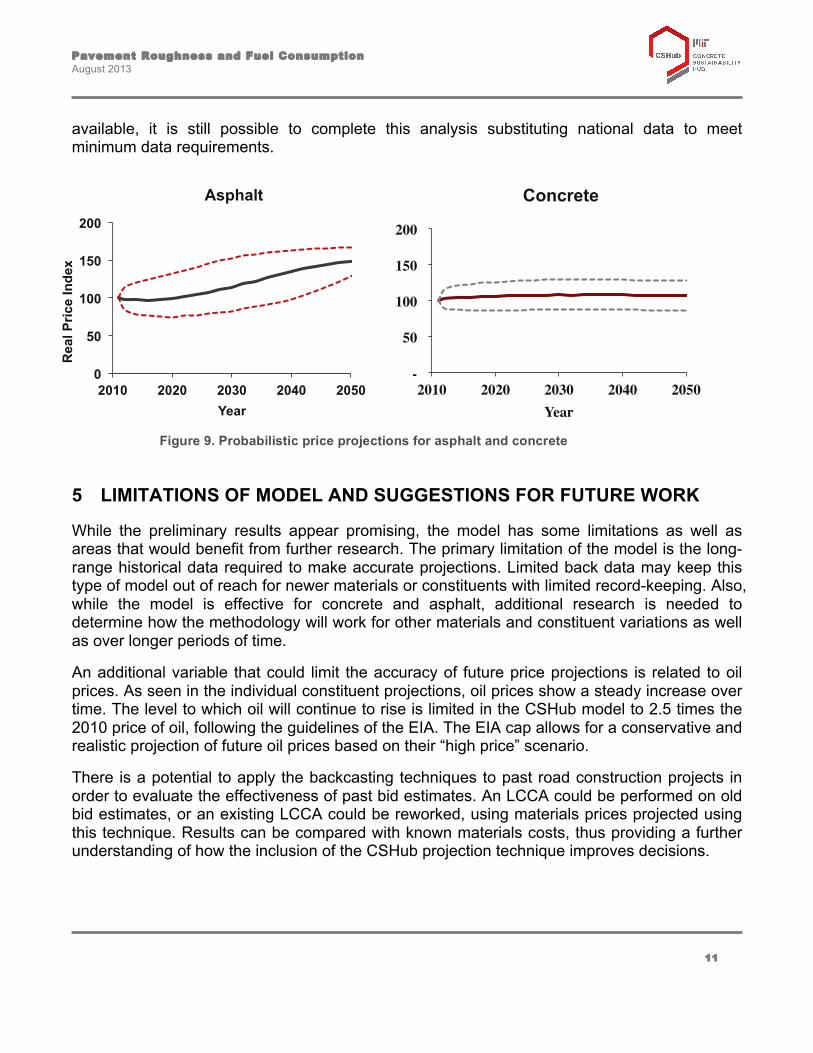
Using the method described above, the price of concrete and asphalt are probabilistically simulated between 2010 and 2050, as shown in Figure 9. The dotted lines surrounding the trendline represent the uncertainty around the projection, at the 5th and 95th percentile, similar to the Cone of Uncertainty used for hurricanes.

Initial model results for the pavement constituents are overall positive when compared to existing modeling mechanisms. When employing 35 years of historical data, the CSHub model was found to outperform the current, “no change in real price” model in most, but not all, constituent price projections. When 60 years of historical data is used to make constituent projections, the CSHub model was found to outperform other existing models. The exact amount of historical data required will depend on the specific materials in the analysis and the available historical data for creating the forecast. In the case where limited state or local data is

Figure 8. Price projections are validated by backcasting from past dates

50

70

90

110

130

1900 1920 1940 1960 1980 2000

Rea

l Pri

ce o

f C

emen

t (1

998’

$)

Year

Cement

Backcasting Projections


11

available, it is still possible to complete this analysis substituting national data to meet minimum data requirements.

5 LIMITATIONS OF MODEL AND SUGGESTIONS FOR FUTURE WORK

While the preliminary results appear promising, the model has some limitations as well as areas that would benefit from further research. The primary limitation of the model is the long-range historical data required to make accurate projections. Limited back data may keep this type of model out of reach for newer materials or constituents with limited record-keeping. Also, while the model is effective for concrete and asphalt, additional research is needed to determine how the methodology will work for other materials and constituent variations as well as over longer periods of time.

An additional variable that could limit the accuracy of future price projections is related to oil prices. As seen in the individual constituent projections, oil prices show a steady increase over time. The level to which oil will continue to rise is limited in the CSHub model to 2.5 times the 2010 price of oil, following the guidelines of the EIA. The EIA cap allows for a conservative and realistic projection of future oil prices based on their “high price” scenario.

There is a potential to apply the backcasting techniques to past road construction projects in order to evaluate the effectiveness of past bid estimates. An LCCA could be performed on old bid estimates, or an existing LCCA could be reworked, using materials prices projected using this technique. Results can be compared with known materials costs, thus providing a further understanding of how the inclusion of the CSHub projection technique improves decisions.

0

50

100

150

200

2010 2020 2030 2040 2050

Rea

l Pric

e In

dex

Year

Asphalt

-

50

100

150

200

2010 2020 2030 2040 2050 Year

Concrete

Figure 9. Probabilistic price projections for asphalt and concrete


12

6 CONCLUSION

As federal and state budgets continue to tighten, the ability to effectively estimate future materials’ prices is more important than ever. For road construction projects, estimates for initial construction costs are commonly created up to a year before the project is constructed. LCCA is often used to estimate decade’s worth of future costs, but the projections of materials’ prices frequently fall short, leading to potentially costly overruns. As such, the present and future costs of road construction projects are often resting on a series of unsure estimations.

The CSHub’s model demonstrates a potential to improve future cost projections as compared to the widely-used “no-change” models and allow for its implementation in practice. The model provides an effective way to probabilistically estimate the future price of a material, concrete and asphalt in this case, based on the fluctuation in the historic prices of the material’s constituents. In order to provide an effective projection, it appears that a minimum of 60 years of historical data for pavement constituents or paving materials is required. This level of constituent data is widely available at the national level, which states can use to relate national prices to their unique situations. This represents a significant limitation of the model in terms of its application to other materials; not all materials will have this level of back data available.

A price projection model that considers uncertainty will help governments to make sound choices in the design phase of a roadway project, lowering the risk of unpredicted project costs in the future. Understanding future materials prices can help officials to make strategic choices in light of limited budgets. For example, a township with many roads to maintain may choose to spend more today to create a lower-maintenance road in order to lessen long-term maintenance costs. Similarly, a government with a limited budget and a road that must be built may choose a road design with a lower upfront cost even if the maintenance costs are higher. With more accurate material price forecasts, officials can weigh the risks and benefits associated with each option and make informed decisions about the future. As budgets shrink and deficits grow, improving decisions for the future is certainly in all of our best interest.


13

7 REFERENCES (2013). "Overview of BLS Statistics on Inflation and Prices." Retrieved May 28, 2013, from http://www.bls.gov/bls/inflation.htm. (2013). Producer Price Indexes. B. o. L. Statistics. Washington, DC. American Society of Civil Engineers (2013). Report Card for America's Infrastructure. Baker, P. and J. Schwartz (2013). Obama Pushes Plan to Build Roads and Bridges. New York Times. New York. Ball, J. (2013). Nate Silver: ‘Prediction is a really important tool, it’s not a game’. The Guardian. London, UK. Box, G. and N. Draper (1987). Empirical Model-Building and Response Surfaces, Wiley. BP (2012). Statistical Review of Energy Prices, British Petroleum. Chatfield, C. (2003). The Analysis of Time Series: An Introduction, Chapman and Hall/CRC. Cheung, Y.-W. and K. S. Lai (1995). "Lag Order and Critical Values of the Augmented Dickey-Fuller Test." Journal of Business and Economic Statistics 13(3): 277-280. Conti, J. J. (2011). Annual Energy Lookout 2011 with Projections to 2035. U. E. I. Administration. Washington, DC. Elder, J. and P. E. Kennedy (2001). "Testing for Unit Roots: What Should Students Be Taught?" Journal of Economic Education 32(2): 137-146. Federal Highway Administration (2013). Annual Vehicle Miles Traveled in the U.S. Washington, DC. Flyvbjerg, B., M. Skamris, et al. (2003). "How common and how large are cost overruns in transport infrastructure projects?" Transport Reviews 23(1): 71-88. Froot, K. A. and K. Rogoff (1994). "Perspectives on PPP and Long-Run Real Exchange Rates." NBER Working Paper Series(4952).

Gransberg, D. D. and C. Rierner (2009). "Impacts of Inaccurate Engineer's Estimated Quantities on Unit Price Contracts." Journal of Construction Engineering and Management 135(11).

Hwang, S., M. Park, et al. (2012). "Automated Time-Series Cost Forecasting System for Construction Materials." Journal of Construction Engineering and Management 138(11): 1259-1269. Kaliba, C., M. Muya, et al. (2008). "Cost escalation and schedule delays in road construction projects in Zambia." International Journal of Project Management 27: 522-531. Kelly, T. and G. Matos (2013). Historical Statistics for Mineral and Material Commodities in the United States. U. G. Survey. Washington, DC.


14

Killian, L. (2001). "Impulse Response Analysis in Vector Autoregressions with Unknown Lag Order." Journal of Forecasting 20(3): 161-179. Leybourne, S. J. and P. Newbold (1999). "The Behavious of Dickey-Fuller and Phillips-Perron Tests Under the Alternative Hypothesis." Econometrics Journal 2: 92-106. Liew, V. K. S. (2004). Which Lag Length Selection Criteria Should We Employ? Economic Bulletin, Venus Khim−Sen Liew. 3: 1-9. National Hurricane Center (2009). Technical Summary of National Hurrican Center Track and Intensity Models. N. O. a. A. Administration. Washington, DC. Odeck, J. (2003). "Cost overruns in road construction -- what are their sizes and determinants?" Transport Policy(11): 43-53. Office of Energy Analysis (2012). Petroleum Market Model of the National Energy Modeling System: Model Documentation 2012. U. E. I. Administration. Washington, DC. One Financial Markets. (2013). "UK Brent Oil." Retrieved May 7, 2013, from http://www.onefinancialmarkets.com/market-library/uk-brent-oil. Perron, P. (1988). "Trends and Random Walks in Macroeconomic Time Series - Further Evidence From a New Approach." Journal of Economic Dynamics and Control 12(2): 297-332. Pindyck, R. S. (1999). "The Long-Run Evolution of Energy Prices." The Energy Journal 20(2): 1-27. Ramberg, D. J. (2010). The Relationship Between Crude Oil and Natural Gas Spot Prices and its Stability Over TIme. Master of Science, Massachusetts Institute of Technology. Rangaraju, P., S. Amirkhanian, et al. (2008). Life Cycle Cost Analysis for Pavement Type Selection. South Carolina, Clemson Univeristy. Reed, J. and J. Rall (2011). Dropping revenue from the fuel tax poses a dilemma for how to pay for maintaining and improving roads and bridges. Washington, DC, National Conference of State Legislation. Schwartz, J. (2013). Governments Look for New Ways to Pay for Roads and Bridges. New York Times. New York City. Swei, O., J. Gregory, et al. (2013). "Backcasting of Construction Related Materials: Testing the Validity of Projecting Future Material Prices over Extended Time Horizons." Submitted to Journal of Construction Engineering and Management. Swei, O., J. Gregory, et al. (2013). "Developing Paving Material Price Projection Models for Incorporation in Life Cycle Cost Analysis." Submitted to Journal of Construction Engineering and Management US General Accounting Office (1997). Transportation Infrastructure: Managing the Costs of Large-Dollar Highway Projects. Washington, DC. Xiarchos, I. M. (2006). Three Essays in Environmental Markets: Dynamic Behavior, Market Interactions, Policy Implications. Doctoral Thesis, University of West Virginia.


15

APPENDIX A

This section provides a more technical description of the methods used within this technique. A full description of the technique is available from (Swei, Gregory et al. 2013; Swei, Gregory et al. 2013).

Step One: Gather data on the historical price trends of asphalt, concrete, and their constituents. In conducting any econometric analysis, it is important to understand if the data exhibits stationary or non-stationary characteristics, as time-series can only be “cointegrated” if they follow the same underlying process. By deciding a time-series is non-stationary, it implies the average value shifts over time, whereas stationary indicates the time-series tends to shift randomly around a single mean value (Chatfield 2003).

One method to assess if a time-series is stationary or non-stationary is to test if a unit-root exists. A unit-root represents an autoregressive process, which will be expanded upon briefly, whose autoregressive coefficient equals one. If a time-series does, in fact, have a unit root, it suggests that the data exhibits autocorrelation (i.e. exhibits a trend) and can be classified as non-stationary (Ramberg 2010). To test the order of integration for a non-stationary time-series, a unit root test can be conducted for each difference of the time-series until it exhibits no unit-roots and can therefore be classified as stationary. As an example, if a time-series must be differenced twice until it is stationary, it can be said that the data is integrated to the second order. Two of the more common tests are the Augmented Dickey-Fuller and Phillips-Perron tests (Leybourne and Newbold 1999). For this research, the Augmented Dickey-Fuller (ADF) test is used to test if the relevant data sets are stationary or not.

The Augmented Dickey-Fuller Test

The basis of the ADF test is an ARIMA (p, d, q) model, where p is the number of autoregressive terms, d is the number of non-seasonal differences, and q is the number of moving average terms. More generally, a time-series, P, is defined by:


16

P! 1− α!

!

!!!

L! (1− L)!

= C+ ε! 1− β!

!

!!!

L!

7.1.1.1.1 (1)

where Pt and εt is the price and error terms in year t, α and 𝛽 represent the coefficients of the autoregressive and moving average terms, C is a constant drift term, and L is the lag operator, meaning:

P!L! = P!!! (2)

ε!L! = ε!!! 7.1.1.1.2 (3)

The ADF tests the null hypothesis of a non-stationary, autoregressive process with a trend against a stationary, autoregressive model that is constant over time. In other words, an ARIMA (p, 1, 0) is the null-hypothesis, and is compared to an ARIMA (p+1, 0, 0) process (Cheung and Lai 1995). The regression equation of the ADF test is as follows:

∆P! = C+ λt+ δP!!! + θ!∆P!!! + ε!

!!!

!!!

7.1.1.1.3 (4)

where ΔPt is the first difference operator, C is a constant, θ is the deterministic time trend, δ is the stochastic time trend, and ε represents the white noise of the process. For the given regression equation, there are three types of ADF tests that may be conducted, as will be expanded upon. For simplification, if we assume there is only one auto-regressive term:

ΔP! = δP!!! + λt+ C+ ε! 7.1.1.1.4 (5)

If γ is equal to zero the process is non-stationary. That is, the time-series growth is independent upon its price level in year t-1, and will grow at some rate (αt + C) with some error term to account for the uncertainty, acting as the equivalent of a random walk. On the other hand, if γ is less than zero, future growth is dependent upon the current position of the process. This implies if the position in year t is high, it is likely growth in year t-1 will turn downward, consistent with what one would expect if a process exhibits mean-reversion.


17

The ADF test will test the null-hypothesis of γ being equal to zero (i.e. unit-root). If one cannot reject the null hypothesis of γ equaling zero, the process is non-stationary, and therefore one will have to “difference” the time-series to make it stationary.

Testing Issues

One underlying issue with the ADF test is that three separate tests can be conducted, where the first two tests are simply the third test with α and/or 𝛽 set equal to zero:

1) Unit-root test with no constants: ΔP! = δP!!! + ε! 2) Unit-root test with drift: ΔP! = δP!!! + C+ ε! 3) Unit-root test with drift and a deterministic time trend: ΔP! = δP!!! + λt+ C+ ε!

Selecting which test to conduct is not necessarily intuitive and can have tremendous implications on test results. Several papers have attempted to address this issue, and so this paper has adopted one of them to increase the likelihood of the correct process being selected (Elder and Kennedy 2001):

• Conduct a t-test for case 3: ΔP! = δP!!! + λt+ β+ ε! o If the presence of a unit-root (δ=0) cannot be rejected, it becomes obvious a unit-

root exists. § If this is the case, it is almost certain that α=0, as studies have shown it is

nearly impossible for a time-series to have a unit-root and have α not equal 0 (Perron 1988).

o If the presence of a unit-root (δ=0) is rejected, it implies the time-series is stationary. This is highly likely in this case given that, as will be discussed briefly, unit-root tests can lack power in detecting if a process is stationary.

§ To understand if there is a deterministic time-trend or not, a unit-root test can subsequently be conducted imposing the constraints in case 2

• f this null hypothesis of a unit-root is also rejected when the constraint of λ=0 is imposed, we can say the time-series is stationary with a drift.

It should be emphasized again that the above description only includes one autoregressive term. The number of autoregressive terms that should actually be included will typically be selected by using some form of a best-fit metric such as the Akaike Information Criterion (AIC) or Bayesian Information Criterion (BIC) (Liew 2004).

Underlying Weakness of the ADF test


18

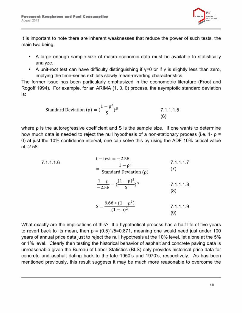
It is important to note there are inherent weaknesses that reduce the power of such tests, the main two being:

• A large enough sample-size of macro-economic data must be available to statistically analyze.

• A unit-root test can have difficulty distinguishing if γ=0 or if γ is slightly less than zero, implying the time-series exhibits slowly mean-reverting characteristics.

The former issue has been particularly emphasized in the econometric literature (Froot and Rogoff 1994). For example, for an ARIMA (1, 0, 0) process, the asymptotic standard deviation is:

Standard Deviation ρ = (

1− ρ!

S ).! 7.1.1.1.5 (6)

where ρ is the autoregressive coefficient and S is the sample size. If one wants to determine how much data is needed to reject the null hypothesis of a non-stationary process (i.e. 1- ρ = 0) at just the 10% confidence interval, one can solve this by using the ADF 10% critical value of -2.58:

7.1.1.1.6 t− test = −2.58

= 1− ρ!

Standard Deviation (ρ) 7.1.1.1.7 (7)

1− ρ−2.58 = (

1− ρ !

S ).! 7.1.1.1.8 (8)

S =

6.66 ∗ (1− ρ!)(1− ρ)! 7.1.1.1.9

(9)

What exactly are the implications of this? If a hypothetical process has a half-life of five years to revert back to its mean, then ρ = (0.5)1/5=0.871, meaning one would need just under 100 years of annual price data just to reject the null hypothesis at the 10% level, let alone at the 5% or 1% level. Clearly then testing the historical behavior of asphalt and concrete paving data is unreasonable given the Bureau of Labor Statistics (BLS) only provides historical price data for concrete and asphalt dating back to the late 1950’s and 1970’s, respectively. As has been mentioned previously, this result suggests it may be much more reasonable to overcome the


19

sample size issue by analyzing the behavior of the constituents, given that this data has been tracked as early as 1870.

In the case, which is likely, that the ADF test cannot detect a stationary process, an alternative testing procedure could be to estimate the parameters of a stationary, first-order auto-regressive process ARIMA (1, 0, 0) to understand if a time-series is stationary or not:

P! = ρP!!! + µμ+ ε 7.1.1.1.10 (10)

Since a stationary process is by definition mean-reverting, it is equivalent to an Ornstein-Uhlenbeck process which reverts to a constant mean, based upon the following stochastic differential equation:

dP! = K(µμ− P!)dt+ σdtW! 7.1.1.1.11 (11)

where K is the speed of mean-reversion, µ is the mean value the process tends to revert to, σ represents the volatility, and Wt is the Brownian motion, or unexplained variation, of the process. The discretized form of the above process is:

P! − P!!! = K(µμ− P!!!)+ σN(0,1) 7.1.1.1.12 (12)

Moving terms around leads to the following:

P! = 1− K P!!! + Kµμ+ σN(0,1) 7.1.1.1.13 (13)

Therefore, if one estimates the parameters of an ARIMA (1, 0, 0) process, the rate of mean-reversion is simply 1-ρ, meaning that if ρ is nearly one, the time-series exhibits nearly no reversion to a mean. It is important to consider that it is possible for the rate of reversion for certain commodities to take up to a decade or more to occur (Pindyck 1999).


20

Step Two: Determine whether pavement constituents exhibit similar trends to asphalt or concrete.

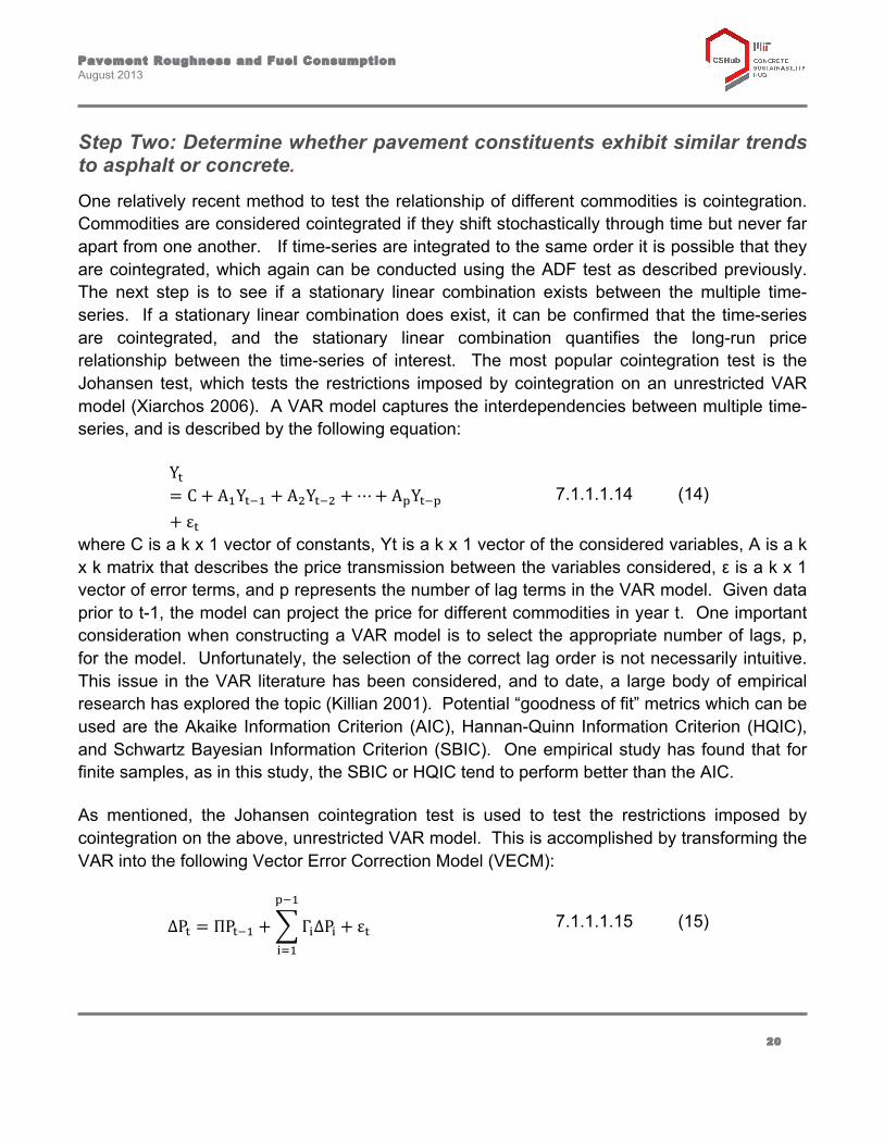
One relatively recent method to test the relationship of different commodities is cointegration. Commodities are considered cointegrated if they shift stochastically through time but never far apart from one another. If time-series are integrated to the same order it is possible that they are cointegrated, which again can be conducted using the ADF test as described previously. The next step is to see if a stationary linear combination exists between the multiple time-series. If a stationary linear combination does exist, it can be confirmed that the time-series are cointegrated, and the stationary linear combination quantifies the long-run price relationship between the time-series of interest. The most popular cointegration test is the Johansen test, which tests the restrictions imposed by cointegration on an unrestricted VAR model (Xiarchos 2006). A VAR model captures the interdependencies between multiple time-series, and is described by the following equation:

Y!= C+ A!Y!!! + A!Y!!! +⋯+ A!Y!!!+ ε!

7.1.1.1.14 (14)

where C is a k x 1 vector of constants, Yt is a k x 1 vector of the considered variables, A is a k x k matrix that describes the price transmission between the variables considered, ε is a k x 1 vector of error terms, and p represents the number of lag terms in the VAR model. Given data prior to t-1, the model can project the price for different commodities in year t. One important consideration when constructing a VAR model is to select the appropriate number of lags, p, for the model. Unfortunately, the selection of the correct lag order is not necessarily intuitive. This issue in the VAR literature has been considered, and to date, a large body of empirical research has explored the topic (Killian 2001). Potential “goodness of fit” metrics which can be used are the Akaike Information Criterion (AIC), Hannan-Quinn Information Criterion (HQIC), and Schwartz Bayesian Information Criterion (SBIC). One empirical study has found that for finite samples, as in this study, the SBIC or HQIC tend to perform better than the AIC.

As mentioned, the Johansen cointegration test is used to test the restrictions imposed by cointegration on the above, unrestricted VAR model. This is accomplished by transforming the VAR into the following Vector Error Correction Model (VECM):

∆P! = ΠP!!! + Γ!∆P! + ε!

!!!

!!!

7.1.1.1.15 (15)


21

Π = A! − I!

!

!!!

and Γ! = A!

!

!!!!!

7.1.1.1.16 (16)

where I is the identity matrix while all other terms remain the same as in the VAR model. If the coefficient matrix, Π, reduces in rank order, r, than it can be said that there are r cointegration relationships amongst the variables of interest. From the VECM, a stationary linear combination of the variables that are cointegrated can be derived. This linear combination describes the long-run price equilibrium between, in this case, constituents and paving materials, and can be used in forecasting future prices of paving materials in the absence of significant historical data for paving commodities.

Step Three: Project the future price of pavement constituents and materials.

Depending upon the characterization of historical data for the time-series of interest, multiple forecasting techniques are available. For this research, if a time-series exhibits “stationary” characteristics, as previously described, the time-series is assumed to follow an ARIMA (1, 0, 0) process. Although this analysis could further study the number of lags to incorporate through a best-fit measure, only one lag is incorporated (Liew 2004). This is both simpler and reasonable given that the proposed application for this work is for projecting prices decades, not years, into the future, which should reduce the implication of only selecting one lag.

In the case, however, a process has historically behaved non-stationary, a Geometric Brownian Motion (GBM) model is selected, which is one possible model to represent this behavior. This acts as a random walk, but with an additional drift term which allows the process to account for the directionality of the time-series, and is described by the following discretized equation:

P! = P!!!e!!!!!

! 7.1.1.1.17 (17)

where Pt is the price in year t, µ and σ represent the logarithmic growth rate and standard deviation (volatility measure), and Wt is standard Brownian Motion, and serves to act as a random walk. Parameters can be estimated by transforming the dataset into logarithmic form and calculating the sample’s differenced average and standard deviation.

A unique input for the price of construction commodities is oil, which plays a particularly important role in the price of paving materials, as bitumen is a by-product of crude oil production. Therefore, a more advanced forecasting model has been constructed in order to account for its unique price behavior.


22

Forecasting Oil – A Unique Forecasting Model

As shown in Figure 2, the detrended historical price for oil has exhibited two characteristics, as discussed by Pindyck (Pindyck 1999). First, the real price of oil over the past 130 years has tended to exhibit mean reversion to a continually shifting mean, which represents the continually shifting marginal cost for oil production. This reversion has taken the form of a quadratic function, which intuitively makes sense; initial oil production became cheaper as technology improved, but as supply, demand, and cost to extract have increased over time, so too has the marginal cost. Second, the time it takes for the price of oil to revert back to its marginal cost can take up to a decade. Due to its monopoly type nature, the price of oil has experienced short-run prices that are extremely volatile and do not match expected competitive prices. Eventually those prices do revert back to competitive levels, and given that pavement rehabilitations occur decades into the future, this time to reversion should not be an issue given the intended application of this research.

Figure 2 Detrended real-price of crude oil over time (BP 2012)

Based upon these characteristics, an appropriate model as discussed by Pindyck is a Ornstein-Uhlenbeck mean-reverting process, as was shown previously (Pindyck 1999). If the process reverts back a mean-value that shifts over time in a quadratic fashion, it equates to the following:

0

0.5

1

1.5

2

2.5

1870 1890 1910 1930 1950 1970 1990 2010

Log

of

Rea

l Pri

ce (

2011

$'s

)

Year


23

C = αt! + βt+ µμ− P! 7.1.1.1.18 (18)

dP! = KCdt+ ε! 7.1.1.1.19 (19)

where K is the speed of mean-reversion, C is the quadratic ally shifting mean-value the process tends to revert to, and εt represents the unexplained noise of the process Pindyck builds upon this general model by considering a multivariate case that allows for fluctuations in both level and slope. These fluctuations in level and slope represent unobservable states in the data set, which is reasonable considering drivers of price such as demand and supply are unobservable, and are represented by each of them being their own Ornstein-Uhlenbeck processes:

dP! = (KC+ λ!Y+λ!Zt)dt+ σdtW! 7.1.1.1.20 (20)

where in addition to the previous terms, Y and Z are themselves their own, Ornstein-Uhlenbeck process, such that:

dY = δ!Ydt+ ε! 7.1.1.1.21 (22)

dZ = δ!Zdt+ ε! 7.1.1.1.22 (23)

Combining all terms in the discretized case leads to the following solution:

P!= C! + C!t+ C!t! + C!P!!! + θ!,! + tθ!,!+ ε!"

(24)

θ!,! = C!θ!,!!! + ε!" 7.1.1.1.23 (25)

θ!,! = C!θ!,!!! + ε!" 7.1.1.1.24 (26)

Step Four: Validate price projections through backcasting. The scope of this analysis only includes a limited number of simple models with low resource and time requirements in order to conduct this analysis for the hundreds of samples analyzed.


24

This presents an opportunity for future work to use more complex models to quantify the value they could potentially add to increasing precision. Nevertheless, it would be promising if it could be shown that one can better project the future relative to a no-change model with even just a few simple models. If a sample exhibits “stationary” characteristics, the aforementioned Ornstein-Uhlenbeck mean-reverting model will be used. In the case, however, a process exhibits non-stationary characteristics, a Geometric Brownian Motion (GBM) model is selected. This acts as a random walk, but with a drift term included as well, as shown in following stochastic differential equation: dP_t=µP_t dt+σP_t dW_t (7) where Pt is the stochastic process, µ and σ represent the logarithmic growth rate and standard deviation (volatility measure), and Wt is standard Brownian Motion, and serves to act as a random walk. Ignoring the uncertainty, the discretized form of the process is: P_t=P_(t-1) e^(µ+1/2 σ^2 ) (8) Parameters can be estimated by calculating the average logarithmic growth rate (i.e. ln Pt – ln Pt-1). The last model this research has considered is a real-price growth factor model (i.e. real inflation rate), but the results are not presented given the GBM is the more prevalent of the two types of simple models. It should also be noted that for all models, the error terms have been omitted since this research is focused upon the accuracy of the forecast and not whether the future price fell within a specified confidence interval.

back to the future: using historic data to improve ......back to the future: using historic data to...

Documents