FERMILAB-PUB-14-289-A

Prepared for submission to JCAP

Background model systematics for theFermi GeV excess

Francesca Calore,a Ilias Cholisb and Christoph Wenigera

aGRAPPA, University of Amsterdam, Science Park 904, 1090 GL Amsterdam, NetherlandsbFermi National Accelerator Laboratory, Center for Particle Astrophysics, Batavia, IL 60510,USA

E-mail: f.calore@uva.nl, cholis@fnal.gov, c.weniger@uva.nl

Abstract. The possible gamma-ray excess in the inner Galaxy and the Galactic center (GC)suggested by Fermi -LAT observations has triggered a large number of studies. It has beeninterpreted as a variety of different phenomena such as a signal from WIMP dark matterannihilation, gamma-ray emission from a population of millisecond pulsars, or emission fromcosmic rays injected in a sequence of burst-like events or continuously at the GC. We presentthe first comprehensive study of model systematics coming from the Galactic diffuse emissionin the inner part of our Galaxy and their impact on the inferred properties of the excessemission at Galactic latitudes 2 < |b| < 20 and 300 MeV to 500 GeV. We study boththeoretical and empirical model systematics, which we deduce from a large range of Galacticdiffuse emission models and a principal component analysis of residuals in numerous testregions along the Galactic plane. We show that the hypothesis of an extended sphericalexcess emission with a uniform energy spectrum is compatible with the Fermi -LAT data inour region of interest at 95% CL. Assuming that this excess is the extended counterpart of theone seen in the inner few degrees of the Galaxy, we derive a lower limit of 10.0 (95% CL) onits extension away from the GC. We show that, in light of the large correlated uncertaintiesthat affect the subtraction of the Galactic diffuse emission in the relevant regions, the energyspectrum of the excess is equally compatible with both a simple broken power-law of breakenergy Ebreak = 2.1 ± 0.2 GeV, and with spectra predicted by the self-annihilation of darkmatter, implying in the case of bb final states a dark matter mass of mχ = 49+6.4

−5.4 GeV.

arX

iv:1

409.

0042

v1 [

astr

o-ph

.CO

] 2

9 A

ug 2

014

Contents

1 Introduction 2

2 Data analysis 42.1 Data selection 42.2 Statistical framework 52.3 Adopted templates 7

3 Galactic diffuse emission models 93.1 Building GDE models with Galprop 103.2 The explored parameter space 133.3 Discussion about the template approach 16

4 Non-parametric analysis of the Galactic center excess 204.1 Theoretical model systematics 204.2 Empirical model systematics 25

4.2.1 Analysis of test regions along the Galactic disk 264.2.2 The covariance matrix of empirical model systematics 274.2.3 Other systematics and the GCE spectrum 28

4.3 The morphology from ten sky segments 29

5 Parametric fits to the Galactic center excess 315.1 Spectral fits with correlated errors 345.2 Dark Matter models 345.3 Astrophysical models 36

6 Discussions 386.1 Astrophysical interpretations 386.2 A signal from dark matter annihilation? 416.3 The energy spectrum at sub-GeV energies 42

7 Conclusions 43

A Description of Galactic diffuse models 46

B Further properties of the Galactic center excess 51B.1 Characterization of the morphology 51B.2 Correlation with Fermi bubbles 52

C Systematic uncertainties 54C.1 An analytical model for the empirical model uncertainty 54C.2 Various method uncertainties 55

D Miscellaneous 56

– 1 –

1 Introduction

The study of Galactic cosmic rays (CRs) and gamma-ray physics has been a very activefield in the last few decades with the launch of PAMELA [1, 2], AMS-02 [3] aboard theInternational Space Station (ISS) and, in particular, of the Large Area Telescope (LAT)aboard the Gamma-Ray Space Telescope (Fermi) [4]. The latter has produced the mostdetailed maps of the gamma-ray sky ever, in a wide energy range and with good energy andangular resolution [5]. The interaction of Galactic CRs with the interstellar medium (ISM)results in the diffuse emission from the Milky Way, which is the brightest source of gammarays seen with the Fermi -LAT. Thus, the Fermi -LAT data provide an important handle forunderstanding the origin and the propagation of CRs in our Galaxy. This is complementedby measurements in microwaves [6, 7], X-rays [8], lower energy [9] and higher energy gammarays [10–12], and neutrinos [13].

More specifically, focused studies of known Galactic sources in gamma rays by both theFermi -LAT and Atmospheric Cherenkov Telescopes (ACTs), together with measurements inX-rays, microwaves and now neutrinos, have helped us in studying and modeling the sourceproperties and the primary CRs composition injected [14–22] by for example supernova rem-nants (SNRs) and pulsars. Moreover, the analysis of gamma-ray data has led to the discoveryof the Fermi bubbles [23, 24], which are believed to be the inverse Compton scattering (ICS)counterpart [23] of the WMAP haze [25, 26], recently observed also with Planck [27].

In addition, the unprecedented energy and angular resolution of Fermi -LAT, combinedwith an energy range of more than three orders of magnitude (30 MeV to 500 GeV) and thelarge field of view, have led to a revolution in the measurement of the gamma-ray propertiesfor specific classes of objects such as active Galactic nuclei [28, 29], star-forming galaxies [30–32] and millisecond pulsars (MSPs) [33–35]. For the latter class of objects very few detectionsand even fewer spectral measurements had been made at gamma-ray energies. Those sameproperties of the LAT instrument have also facilitated an unprecedented measurement of theisotropic gamma-ray background (IGRB) [36, 37] and, for the first time, of its power-spectrum[38]. These measurements have improved our understanding of extragalactic astrophysicalobjects [32, 37, 39–41] and ultra-high-energy CRs [42–44].

A wide range of cosmological and astrophysical observations have shown that about 85%of the matter content in the Universe is non-baryonic, dark and cold [45]. The currently lead-ing candidates for this dark matter (DM) are Weakly Interacting Massive Particles (WIMPs),which appear in a large number of scenarios of beyond-the-Standard Model physics [46–48].The ‘freeze-out mechanism’ that sets their abundance in the early Universe provides clearpredictions for the self-annihilation rate of these particles today. Their annihilation productscould contribute to the cosmic- and gamma-ray fluxes observed at Earth with rates that aretantalizingly close to the sensitivity of current experiments.

Recently, a number of groups searching for DM signals have analyzed the gamma-rayemission from the inner few degrees around the Galactic center (GC), and either claimed [49–56] or refuted [57] the existence of an extended diffuse and spherical emission componenton top of the standard astrophysical backgrounds. It was found that the excess emissionis compatible with a radial volume emissivity profile ∝ r−Γ, with Γ in the range 2.2 [52] to2.4 [53], and with r denoting the Galacto-centric distance. Furthermore, it was demonstratedthat the excess features an energy spectrum that peaks at a few GeV and is broadly consistent

– 2 –

with a signal from DM annihilation, although other source spectra (a log-parabola or a power-law with exponential cutoff) can be accommodated by the data, see e.g. refs. [50, 53, 54].

However, the modeling of the Galactic diffuse emission (GDE) is very uncertain in theinner few hundred pc of the GC (150 pc projected distance corresponds to about 1), andis strongly affected by systematics related to point source subtraction and the modeling ofdiffuse backgrounds [54, 57, 58]. Complementary observations, like local measurements ofCRs, are not able to set strong constraints on the CR propagation properties or gas densitiesin that region. Moreover, the magnetic field intensity can be only indirectly constrained bythe synchrotron emission at microwaves (or the dispersion measures) for given assumptionson high (low) energy electrons. Indeed, given the high density of astrophysical objects andCRs at the GC, and the unprecedented sensitivity of Fermi -LAT, it seems far from surprisingthat residuals were found above the astrophysical emission that had been anticipated [58, 59].

If the observed GC excess is indeed caused by the annihilation of DM particles (whichis a very exciting but also exotic possibility), it should visibly extend tens of degrees aboveand below the GC [60, 61]. The solid confirmation of an excess emission with the samespectral properties as observed in the inner few degrees around the GC is hence a necessary(though not sufficient) criterion for the interpretation of the excess at the GC in terms ofDM annihilation, and as such of utmost importance. The first claim that such an extensionto high latitudes, up to tens of degrees, is indeed observed in the Fermi -LAT data (mostnotably in the Fermi bubble regions [24], which happen to have a good signal-to-noise forDM signals), was put forward in ref. [62], and reproduced in refs. [55, 63]. Nonetheless, alsothis high latitude region is extremely difficult to analyze, mainly because of the dominantbackground represented by gamma rays originating from the interactions of CRs with theISM and photon fields.

Besides its status as a “compelling case for annihilating DM” [55], the GC excess emis-sion has also been interpreted in terms of various astrophysical processes. Firstly, the excessgamma-ray emission could originate from a population of gamma-ray MSPs associated withthe central stellar cluster and not yet detected by the Fermi -LAT [54, 64–66] (as already sug-gested in ref. [67] years ago using EGRET data). Recently, several arguments disfavor theMSPs hypothesis, suggesting that only up to 5–10% of the observed emission can originatefrom MSPs [68–70].

Another possible explanation of the GC excess relies on the interactions of CRs with gas,for example non-thermal bremsstrahlung from a population of electrons scattering off neutralmolecular clouds in the inner 2 [71], or interactions between the gas and protons acceleratedby the super-massive black hole sitting at the GC [72]. In general, those mechanisms wouldlead to an excess emission correlated with the gas distribution itself. In particular, the formerprocess could not only explain part of the GeV excess emission in the Galactic ridge region,but also the excess at TeV energies as seen by HESS [73, 74]. However, in both cases anextended signal up to a few kpc is excluded, unless a large amount of unidentified sphericallydistributed gas is present at the GC. It has also been suggested that burst-like events duringan active past of our Galaxy may represent a viable mechanism for producing gamma raysin the inner Galaxy with the observed spectrum and morphology. Hadronic [75] or leptonic[76] scenarios might explain some of the observed excess features at high latitudes.

In this paper, we will reanalyze the Fermi -LAT gamma-ray data at high Galactic lat-itudes. We will consider a Region Of Interest (ROI) at Galactic latitudes 2 ≤ |b| ≤ 20

– 3 –

and Galactic longitudes |`| < 20, which we refer to as the inner Galaxy throughout. Thisregion avoids the inner 2 degrees of the Galactic disk, which is the region of the sky thatis most contaminated with strong gamma-ray point sources and large uncertainties in thediffuse emission.

The aims of this paper are the following: i) to robustly confirm the existence of an ex-tended excess emission in the inner Galaxy on top of the standard astrophysical background,henceforth the Galactic center excess (GCE); ii) to characterize its spectral and morpho-logical properties and its status as the extended counterpart of the excess seen at the GC;and iii) to investigate in a comprehensive manner the systematic uncertainties related to themodeling of diffuse backgrounds. To this end, we study theoretical model systematics, whichare related to variations in the different possible models for the GDE, and empirical modelsystematics, which we estimate by an analysis of residuals from a large number of test regionsalong the Galactic disk.

We adopt template-based multi-linear regression techniques to fit the Fermi -LAT datain our ROI. To this end, we model the GDE from the Milky Way based on physical modelsfor the production and propagation of CRs in the Galaxy. By means of the Galprop code, webuild a large set of GDE models with the aim of spanning the full range of possible physicalconditions that affect the gamma-ray emission coming from direction of the inner Galaxy.Each background model is then tested against Fermi -LAT data during the fitting procedure.

Two criteria guide our search for GDE models for the inner Galaxy: a) a good statisticalfit, i.e. small TS values, where TS ≡ −2 lnL throughout; and b) self-consistency, i.e. agree-ment between the predicted and measured levels of the individual GDE components (this isnot guaranteed in a template fit, where spectra can vary arbitrarily).

The paper is organized as follows: In section 2 we discuss the data reduction, thestatistical methods and the modeling of some of the backgrounds. Section 3 is dedicatedto a detailed explanation about how we model the main components of the Galactic diffuseemission. In section 4 we then present the results on the spectrum and morphology of theexcess emission, and estimate theoretical and empirical model systematics. We performparametric fits to the data in section 5, and leave our discussion to section 6. Finally, insection 7 we state our conclusions.

2 Data analysis

In this work, we study gamma rays collected by the Fermi -LAT from the inner Galaxy withtemplate-based multi-linear regression techniques, see e.g. ref. [23, 24]. The main differencewith respect to previous studies is an extensive treatment and discussion of systematics re-lated to the modeling of the GDE, and an incorporation of these uncertainties in the finalspectral and morphological fits to the GCE. In addition, we introduce a few technical im-provements, including a weighted adaptive masking of point sources, the proper treatment ofthe point-spread-function (PSF) of Fermi -LAT, and the non-logarithmic binning of energieswhich facilitates flux measurements at high energies.

2.1 Data selection

In our analysis, we use 284 weeks of reprocessed Fermi -LAT data (starting from 4 Aug2008) with energies between 300 MeV and 500 GeV.1 We apply the standard zenith-angle

1See http://fermi.gsfc.nasa.gov.

– 4 –

cut θ < 100 in order to avoid contamination from the Earth limb, and the recommendedgtmktime cut (DATA QUAL>0) && (LAT CONFIG==1). To maximize the available number ofphotons at high energies we use front- and back-converted P7REP CLEAN events.2 The ini-tial event selection and the calculation of exposure maps is done using the standard Fermi

ScienceTools v9r32p5 with the instrument response functions (IRFS) P7REP CLEAN V15.We use the healpix projection for the spatial binning of data [78]. The healpix grid is a

hierarchical equal-area iso-latitude pixelization of the sphere, and it is well suited for full-skyanalyses of astronomical data. In our work, we adopt the resolution parameter nsize = 256,which corresponds to a pixel size of 1.598 × 10−5 sr (roughly 0.23 edge length for squarepixels). All mask definitions in this paper refer to the pixel center as defined in the healpix

grid, leading to ± ∼ 0.1 variations at the mask edges.

As noted above, the baseline ROI of this work, which we refer to as inner Galaxy, isdefined as

|`| ≤ 20 and 2 ≤ |b| ≤ 20 , (2.1)

where ` and b are the Galactic longitude and latitude, respectively. As discussed above, thelower latitude cut is applied to reduce contamination with diffuse and point source emissionfrom the Galactic disk. The overall region is kept small (compared to previous analyses [55,62]) in order to avoid biasing our analysis results by potential mis-modeling of the diffuseemission in regions of the sky that are irrelevant for the GCE. However, we will use a numberof additional ROIs for validation tests as well as for estimates of model systematics.

In contrast to previous studies, we use energy bins that increase in logarithmic sizewith energy. This will partially counterbalance the reduced photon statistics that usuallycomplicate the analysis at energies above 10 GeV. To this end, we define energy bins suchthat for a given photon flux with a spectral index of Γ, each bin contains an equal number ofexpected events. For a given energy range E0 ≡ Emin to Emax, and a given number of binsnbins, we find that the boundaries of these energy bins can be recursively determined by

Ej+1 =

(E1−Γj − E1−Γ

min − E1−Γmax

nbins

) 11−Γ

, with j = 0, 1, . . . , nbins . (2.2)

In the present analysis, we use nbins = 20 bins in the range 500 MeV to 500 GeV andadopt the value Γ = 1.45, which is harder than the actual spectrum. This is a compromisebetween a loss in statistics at high energies on the one hand, and unreasonably wide energybins on the other hand. Furthermore, we add four linearly spaced energy bins between 300and 500 MeV.

2.2 Statistical framework

We use the maximum likelihood technique for parameter inference and confidence intervalestimation. To this end, we adopt a weighted Poisson likelihood function for the photondata [79],

− 2 lnL = 2∑i,j

wi,j(µi,j − ki,j lnµi,j) + χ2ext , (2.3)

2We leave an analysis based on a subset of events with better angular resolution at sub-GeV energies forfuture work [77].

– 5 –

where µi,j and ki,j are, respectively, the expected and observed number of photons in the ith

energy bin and jth pixel, and χ2ext allows for external constraints on the model parameters.

The definition of the point source (PSC) mask weights wi,j ∈ [0, 1], as well as of the externalconstraints χ2

ext, will be discussed below.

The expected number of photons is given by the sum of different space- and sometimesenergy-dependent templates that represent: i) the GDE (tying π0 and bremsstrahlung com-ponents together, cf. section 3 for details), ii) the Fermi bubbles, iii) the IGRB, iv) theemission from the detected PSCs in the Fermi -LAT Second Source catalogue (2FGL) [80],and v) a spherically symmetric profile, centered at the GC that accounts for the GCE excessemission (cf. section 2.3). We leave the normalization of each model component free to floatin each energy bin. The total model is defined by

µi,j =∑k

θi,kµ(k)i,j , (2.4)

where θi,k is the normalization of component k in energy bin i, and µ(k)i,j is the predicted

number of events of component k when θi,k = 1.External constraints will be adopted both for the IGRB and for the Fermi bubbles,

which we leave free to float in our analysis, but which can be more efficiently determined inregions outside of our ROI. The constraints are assumed to be Gaussian, such that χ2

ext is ofthe form

χ2ext =

∑i,k

(φi,k − φi,k

∆φi,k

)2

, (2.5)

where φi,k denotes the predicted flux of component k in energy bin i, and φi,k and ∆φi,k arethe externally supplied mean and standard deviation (see section 2.3).

We obtain the best-fit model parameters by minimizing −2 lnL with respect to all pa-rameters, using the minimizer Minuit.3 For the template analysis, we derive error bars fromthe covariance matrix of −2 lnL, and checked that our results remain essentially unchangedwhen using the more accurate (but much more time-consuming) minos algorithm in Minuit.Note that we allow negative values of θi,k in our fits, which improves the stability of Minuitwithout affecting our conclusions.

The finite angular resolution of the LAT is incorporated by following the prescriptiondescribed in ref. [58]. Using healpix, we decompose the skymap into spherical harmonics, re-weight the moments according to the decomposition of the Fermi -LAT PSF (taking the GCas reference position), and then transform them back to sky coordinates. This method is usedfor all diffuse emission components, except the GCE templates (which remains non-smoothedfor simplicity), and the PSC templates (which we instead smooth using the more accurategtmodel from the Fermi ScienceTools). We found that our results are not significantlyaffected by the details of the smoothing (more specifically, neglecting smoothing of the diffusecomponents entirely or smoothing them instead with a fixed-width Gaussian with 2 FWHMinduces changes in the spectra at the % level).

In order to minimize the impact of known point sources on our analysis, we use a ‘soft’PSC mask, with values that can range from zero to one. In practice, this mask acts as an

3See http://seal.web.cern.ch/seal/MathLibs/Minuit2/html/.

– 6 –

energy-dependent re-weighting of the exposure and the associated count numbers in differentregions of the sky. The corresponding reweighting factor, wi,j , enters eq. (2.3) as a simpleprefactor that multiplies the likelihood contributions from individual pixels. In the Gaussianlimit, this corresponds to increasing statistical errors by a factor w−1

i,j .The weights are defined as follows. We infer the expected number of photons from

PSCs, µPSCi,j , in different pixels and energy bins by creating a model map that contains all

point sources of the 2FGL [80], fixing their fluxes to the best-fit parameters of the catalogue.We compare these numbers with the expected number of background events from the GDE(including only the π0, ICS and Bremsstrahlung components at their nominal normalization),µBGi,j . For definiteness, we take the model P.4 The weights are defined by

wi,j =1(

µPSCi,j

fPSC µBGi,j

)αPSC

+ 1

, (2.6)

where fPSC denotes the threshold of the fraction of point source contamination above whicha pixel is masked, and αPSC parameterizes the smoothness of the transition between w = 0and w = 1. As default values, we select αPSC = 5 and fPSC = 0.1. We discuss the systematicsrelated to our choices concerning the PSC mask definition in section 4.1.

We emphasize that we apply the PSC mask only when performing fits and calculatinglikelihood values. The calculation of fluxes integrated over our ROI, as shown in variousfigures throughout the paper, remains unaffected by the PSC mask, in order to simplifycomparison with other work. Furthermore, as described below, we include as a defaulttemplate in all analysis steps the PSC flux derived from all of the 2FGL point sources with anormalization that is fixed to one. By construction, the 2FGL sources do not affect the fitsto the data, but they contribute to the overall flux in our ROI and indicate where PSC arerelevant and where not.

2.3 Adopted templates

The PSC template is derived from the 2FGL [80], as described above. The GDE templateswill be extensively discussed in section 3. We describe here briefly the remaining spatialtemplates that we use in our analysis and highlight their main characteristics.

Fermi bubbles. In our main analysis, we model the emission of the Fermi bubbles asflat within the region defined in ref. [24]. We will discuss the impact of a possible latitudedependence of the Fermi bubbles emission in appendix B.2.

As mentioned in section 2.2, when performing fits in our main ROI, which is relativelysmall and does not include the whole Fermi bubbles template, we introduce an additionalexternal constraint on the bubbles flux implemented as in eq. (2.5). Mean and standarddeviations are taken from measurements in ref. [81], where the errors incorporate systematicsrelated to the uncertainties in the GDE.5

4We refer to appendix A for the definition of model parameters. It represents the reference model ofref. [58].

5During the final stages of our work, the first Fermi bubbles analysis by the Fermi-LAT Collaboration hasbeen released [83]. Data above 10 in latitude have been analyzed and the spectrum and morphology of theFermi bubbles have been derived. Since we do use preliminary results of this analysis to constrain the bubblesspectrum, we do not expect a large variation of our results due to the imposed bubbles spectral shape.

– 7 –

Name Notes Ref.

PSC Spectra fixed to 2FGL [80]Fermi bubbles Flat emission — Spectrum constrained [24, 81]

IGRB Constant emission — Spectrum constrained [37]GCE Generalized NFW profile with inner slope γ –

Ackermann+ GDE models (×13) (π0 + Bremss) + ICS [58]Additional GDE models (×47) (π0 + Bremss) + ICS This work

Table 1. Different templates and models used throughout the analysis. We construct the models inthe bottom row by using the Galprop v54 code [82]. As indicated, in our template analysis we tieboth the bremsstrahlung and π0 components together, “π0+Bremss”, and vary them simultaneouslyby a common factor. Furthermore, we will split the GCE (ICS) templates in 10 (9) different segmentsduring the morphology analysis in section 4.3.

IGRB. Fits within our main ROI do not well constrain the very subdominant IGRB emis-sion. We hence constrain this component – similarly to what we do for the Fermi bubbles– by introducing additional terms in the likelihood function, with mean values and standarddeviations (which include statistical errors and systematical errors from the GDE and othersources) as given in ref. [37].

GCE template. Throughout most of our analysis (except for the morphology studies insections 4 and 5 and appendix. B), we will parametrize the volume emissivity of the GCE interms of the spherically symmetric6 generalized NFW profile, as given by

ρ(r) = ρs(r/rs)

−γ

(1 + r/rs)3−γ , (2.7)

squared. This is clearly motivated by the DM annihilation interpretation of the GCE. Wewill use the common normalization ρ(r) = 0.4 GeV/cm3 at the position of the Sun and ascale radius of rs = 20 kpc to ease of comparison with previous results in the literature. Ifnot stated otherwise, we will furthermore adopt the value γ = 1.2, which is compatible withprevious (see e.g. refs. [55, 62]) and our own findings below.

In general, the gamma-ray flux ( GeV−1 cm−2 s−1 sr−1) from self-conjugate DM particles,χ, annihilating in the Galactic DM halo is given by

dN

dE=〈σv〉

8πm2χ

dNγ

dE

∫l.o.s.ds ρ2(r(s, ψ)) , (2.8)

wheremχ is the DM mass, 〈σv〉 the velocity averaged total annihilation cross-section, dNγ/dEthe averaged energy spectrum of photons produced per annihilation, and ρ(r) the radial DMenergy density distribution as function of the Galacto-centric distance r. The coordinates ≥ 0 runs along the line-of-sight and is related to the distance from the GC by r(s, ψ) =√

(r − s cosψ)2 + (s sinψ)2, where ψ is the angular distance from the GC and r = 8.5 kpcdenotes the distance between Sun and GC.

6Although the DM profile is generally assumed to be spherically symmetric, N-body simulations predictsome degree of tri-axiality of the halos in their inner part, see for example ref. [84] for a recent discussion. Inthis case, an elongation of the DM associated emission would be expected towards a specific direction. Wediscuss the elongation of the measured excess in appendix B.

– 8 –

3 Galactic diffuse emission models

The observed gamma rays with energies above 100 MeV typically originate from CRs thatpropagate in the Galaxy. Firstly, CR nuclei produce via inelastic nucleon-nucleon collisionswith the interstellar gas neutral mesons (mainly π0s), which subsequently decay to gamma-raypairs [82, 85, 86]. This is typically, and throughout this work, referred to as the π0 Galacticdiffuse component. Secondly, CR electrons interact with the interstellar gas, giving rise tobremsstrahlung emission [87–89], which can be a significant diffuse gamma-ray componentbelow a few GeV in the gas-rich regions of our Galaxy. Finally, CR electrons up-scatterlow-energy photons via ICS into the gamma-ray energy regime [89, 90]. ICS, bremsstrahlungand π0 constitute the three components of the GDE. Various ingredients enter the evaluationof these three GDE components, which we will discuss in the remainder of this section.

Firstly, the exact distribution of the CR sources is very important. This is especiallytrue for electrons because they lose energy quickly, such that their distribution in the Galaxy– at higher energies – is strongly correlated to their initial injection (i.e. acceleration andproduction) region.7 In addition, the assumptions on the diffusion scale height of the Galaxy,the diffusion coefficient8 D(= 1

2λc) and its dependence on CR rigidity (which together set thetime scale nuclei of a given rigidity stay in the Galaxy before escaping to the intergalacticmedium) can strongly affect the diffuse components. The large scale assumptions aboutdiffusion, convection and re-acceleration can strongly impact – and are thus constrained by –the CR spectra [91–93] that we measure locally. The same applies for the large scale (angularand spatial) gamma-ray spectra [58, 94, 95], which, in turn, impact any indirect DM search,either in antiprotons [96–98], positrons [99] or gamma-rays [100].

Furthermore, the exact assumptions on the gas distribution in the inner Galaxy, whichis the target of CRs responsible for the π0 and the bremsstrahlung emission, affect in a directmanner the gamma-ray observations. The main constituent of the interstellar gas is theatomic hydrogen (HI) traced by its 21 cm line emission [101, 102], while the other importantcomponent of the ISM gas is the molecular hydrogen (H2), which is traced indirectly by the2.6 mm line emission from CO [103]. Additionally, since CR electrons of energies O(1) GeVand above suffer from fast energy losses due to synchrotron and ICS, the exact assumptionson the magnetic field distribution and the interstellar radiation field (ISRF) in the region ofinterest is of vital importance. In this context, magnetic fields, which have a random and anordered component at every position of the Galaxy, can affect both the synchrotron electronslosses, which are important above few GeV in energy, and the way CRs diffuse especiallyin regions with strong ordered magnetic fields (see ref. [104] for an example on the impactmagnetic fields can have on causing anisotropic diffusion of CRs and its impact on potentialgamma-ray signals from DM). The ISRF assumptions matter for a second reason, namely thefact that those photons are the target of CR electrons that up-scatter them to the observedgamma-ray energy regime.

Emission directly correlated with the GC or the inner Galaxy comes only from the inner1–2 kpc of the Galaxy where the CRs propagation conditions can be very different from thoselocally. For example, one may need to consider the impact of potentially strong convectivewinds that could exist in that region and could be associated to the Fermi bubbles. Moreover,

7CR electrons are of different origin: They are diffusive shock accelerated ISM electrons at SNRs, secon-daries from inelastic pp and pHe collisions (predominantly), and electrons produced in pulsars magnetospheresand further accelerated at the termination shock of Pulsar Wind Nebulae (PWNe).

8Assuming that CRs diffuse isotropically in the Galaxy, λ is the diffusion length.

– 9 –

CR diffusive re-acceleration may be different in that part of the Galaxy compared to the localenvironment. In fact, the propagation conditions in the inner Galaxy can have only a verymild effect on the local CR spectra, which instead depend much more on the assumptionsregarding, for example, the spiral arms (see for instance ref. [105]), and are hence only weaklyconstraint.

In the following subsection we describe how the GDE can be modeled starting from thefundamental ingredients of production and propagation of CRs in the Galaxy. By using theGalprop code and varying the physical parameters at stake, we build a set of GDE modelsin order to explore physical scenarios for such a gamma-ray background. We discuss theparameter ranges that are considered and the main assumptions of this approach. Finally,we will discuss typical template variations that different assumptions on the GDE componentscan lead to.

3.1 Building GDE models with Galprop

In our analysis, we make use of the Galprop v54 code [106–108] to produce gamma-raytemplates for the GDE at various energies. Additionally we download the healpix GDEπ0, bremsstrahlung and ICS component maps from some of the models of ref. [58], whichwere also produced with Galprop v54. We refer for further details to ref. [58]. We willbriefly summarize the properties of the adopted GDE models here, and provide more detailsin appendix A.

CR sources are assumed to be distributed with a rotational symmetry on the disk, withvarying radial dependence. Their distribution can either follow the distribution of SNRs,pulsars, OB stars (see ref. [58]) or combinations of them. The primary CR electrons, protonsand nuclei are then injected into the interstellar medium with a power-law dN/dEkin = E−αkin ,which can vary between species and with kinetic energy (per electron or nucleon) Ekin.9 Forthe Galactic gasses, as we described, there are two major neutral hydrogen components HIand H2 and a subdominant contribution of ionized hydrogen HII. These are all modeled asseparate components, with H2 suffering from the fact that a conversion from CO to H2 hasto be performed (see refs. [103, 107]).10

Diffusion of CRs in the Galaxy is assumed to be homogeneous and isotropic within acylindrical volume of r ≤ rD and |z| ≤ zD, where z and r parametrize the position alongthe longitudinal and polar axes. It is described by a scalar diffusion coefficient depending onrigidity R as

D(R) ≡ Dxx(R) = D0

(R

4GV

)δ, (3.1)

where D0 is the diffusion coefficient at 4 GV and δ is the diffusion index with values between0.3–0.6.11 Diffusive re-acceleration in turn is connected to spatial diffusion through a simplerelation

Dpp(R) =4

3δ(2− δ)(4− δ)(2 + δ)

R2v2A

Dxx(R), (3.2)

9We include all species up to Carbon stable isotopes (Iron for the models of ref. [58]) and take the CRprotons and heavier CR nuclei to have the same injection indices.

10For the GDE models that we built ourselves, we use the conversion factor XCO profile from ref. [109],while the models from ref. [58] come with their own XCO profiles. Given that most of the H2 emission closeto the inner Galaxy is actually masked by our low latitude cut |b| > 2, the precise radial dependence of XCOis of little relevance here.

11δ can vary with rigidity but for our work we keep it fixed to 1/3.

– 10 –

ICS, 1 GeV, ModA

-6.3 -4.52

π0, 1 GeV, ModA

-6.3 -4.52

Bremsstrahlung, 1 GeV, ModA

-6.3 -4.52

Figure 1. Predicted emission for the GDE components of model A. From left to right: ICS, π0, andbremsstrahlung. The fluxes are shown in the 40 × 40 sky-region, centered at the GC and maskingout |b| < 2. The corresponding units are log10(GeV−1 cm−2 s−1 sr−1).

with vA being the Alfven speed.Convection is considered to be taking place perpendicularly away from the Galactic

disk, with the convection velocity being zero on the disk but having a gradient dv/dz. TheGalactic magnetic field responsible for synchrotron losses of CR electrons is assumed to havea cylindrical symmetry with the parametrization

B(r, z) = B0 e(r−r)/rc e−|z|/zc , (3.3)

where B0 is the local magnetic field and rc and zc are the radial and longitudinal extension,respectively (r is 8.5 kpc).

Finally, the ISRF is built from the contribution of many stellar components and includesthe effects of absorption and re-emission from dust grains (see ref. [107] for further detailsand ref. [110] for a description on how it is constructed). Within the code the ISRF is dividedinto three basic components, related to the direct emission from stars, dust grains and CMB.The user is free to vary the normalization of each of these components.

In figure 1, we show the typical morphology of the three different diffuse emissioncomponents at 1 GeV from a model, model A, which has parameters that are defined intable 2. We will refer to model A as our reference model for further discussions, since as wewill see below it well describes the gamma-ray data and spectra in the inner Galaxy. Theleft panel of figure 1 refers to the ICS emission, which is smooth and depends mainly on theelectron distribution and the properties of the B-field and the ISRF. On the other hand, π0

(middle) and bremsstrahlung (right) morphologies trace directly the distribution of the gasand depend mainly on the proton and electron CR densities, as well as on the properties ofCR diffusion, re-acceleration and convection.

The observed emission as shown in figure 1 receives contributions from all distances alongthe line-of-sight. However, whether the overall emission is dominated by locally producedgamma rays (within a few kpc), or by gamma rays from the GC, is a strong function of theGalactic latitude. This is illustrated in figure 2, where we show the fractional contributionsto the GDE components as function of the line-of-sight for a typical GDE model.12 We find

12To generate this figure, we used our own modified version of Galprop 54.1.984 where the line-of-sightintegration can be restricted. We adopted a simple GDE model defined by the galdef file 54 01.

– 11 –

10−2

10−1

3.0%, 0.7%, 7.5% 3.1%

π0, Bremss, ICS total

from GC: ℓ = 0, b = 10

π0

Bremss

ICS

10−2

10−1

5.3%, 1.2%, 10.0% 5.2% ℓ = 0, b = 4

10−2

10−1

100

101

Emissivity 38.7%, 19.8%, 17.2% 35.6% ℓ = 0, b = 0

10−2

10−1

12.3%, 3.2%, 11.4% 11.0% ℓ = 0, b = −4

0 2 4 6 8 10 12 14 16

Line-of-sight distance [kpc]

10−2

10−1

9.5%, 2.5%, 7.7% 8.2% ℓ = 0, b = −10

Figure 2. Typical differential volume emissivity dN/dV/dt/dE (in arbitrary units) of the three GDEcomponents along the line-of-sight at five different Galactic latitudes, zero Galactic longitude, andgamma-ray energies of 2.6 GeV. The numbers show the fraction of π0, bremsstrahlung, ICS and totalemission that comes from the distance range 7.5–9.5 kpc (with the GC being at 8.5 kpc). At latitudesabove |b| ≥ 4, less than about 11% of the total GDE comes from this central region. Note that thereduced amount of local gas in the southern hemisphere leads at negative latitudes to larger relativecontributions from the Galactic center.

that in the case of our baseline ROI, less than 14% (and for |b| ≥ 4 less than 11%) of theGDE actually comes from regions close to the GC. The main challenge in extracting theGCE in the inner Galaxy is hence to characterize the uncertainties and properties of the localgamma ray emissivity.

We close this subsection with a discussion of our model A, which we adopt as a referencemodel throughout. We tuned model A to be “self-consistent” in the sense that, after the fitto the data that we will perform below, the measured and predicted normalizations of theGDE template components agree with high accuracy (see introduction, and see section 4below). The purpose of this model is to constitute a proof-of-principle that shows that sucha self-consistent model is indeed possible with physically not unreasonable parameters.

However, we note that there are significant degeneracies between the physical assump-

– 12 –

Name zD D0 vA dv/dz Source αe(αp) Ne(Np) B-field ISRF

A 4 5.0 32.7 50 SNR 2.43(2.47) 2.03(5.8) 090050020 1.36,1.36,1.0B 4 28.0 31.0 0 SNR 2.43(2.39) 1.00(4.9) 105050015 1.4,1.4,1.0C 4 5.0 32.7 0 SNR 2.43(2.39) 0.40(4.9) 250100020 1.0,1.0,1.0D 4 5.2 32.7 0 SNR 2.43(2.39) 0.40(4.9) 050100020 0.5,0.5,1.0E 4 2.0 32.7 0 SNR 2.43(2.39) 0.40(4.9) 050100020 1.0,1.0,1.0

Table 2. The properties of GDE models A–E. Here, zD is in kpc, while rD is taken to be 20 kpc. D0

is in units of 1028 cm2 s−1, vA is in km s−1 and dv/dz in km s−1 kpc−1. The CR electron and protonnormalizations are Ne(Np) in units 10−9 cm−2 sr−1 s−1 MeV−1 and refer to the differential flux atEkin of 34.5 and 100 GeV. αe and αp are the electron and proton injection indices above rigiditiesof 2.18 and 11.3 GV, respectively (and are respectively equal to 1.6 and 1.89 below these rigidities).For the gas assumptions we take, TS = 150 K and an E(B-V) magnitude cut of 5 (see discussion insection 3.2). For model A the magnetic field “090050020” denotes in eq. (3.3) B0 = 9.0 µG, rc = 5kpc and zc = 2 kpc (similarly for the other models). Finally, the three numbers in the “ISRF” columnrefer to the multiplication factors of the “optical”, “IR” and CMB components of the ISRF modelused in Galprop v54 webrun.

tions that can have a similar impact on the resulting diffuse gamma-ray spectra. For instance,a harder ICS spectrum could be the result of a harder injection spectrum for the CR elec-trons, a lower energy loss rate (due to a reduced B-field), a different rigidity dependence ofthe CR diffusion or a different distribution in the energy density of the ISRF. Thus, we canhave different combinations of physical properties leading to self-consistent models.

Our model A adopts a CR electron normalization that is significantly higher (by a factorof 5) than the typical dNe/dE '0.4×10−9 cm−2 sr−1 s−1 MeV−1 at ∼30 GeV that is requiredto fit the local CR lepton data. In particular, for the ICS emission at GeV scale gamma-rayenergies, the responsible CR electrons have typically energies ∼50 GeV or higher. At theseenergies, the CR electron fluxes are dominated by the contribution of sources within ∼ 1kpcfrom the Sun’s position and are not very sensitive to higher normalizations in the electronflux at few kpc distances. Thus, a higher CR electrons normalization along the line-of-sightand towards the GC is quite well possible. Such a higher flux may be due to some youngor middle aged pulsars that lie along that direction, either in the spiral arms or in the innerpart of the Galaxy. We note that both the adopted B-field and ISRF have relatively highenergy densities. Given the uncertainties along the line-of-sight toward the GC, they are stillviable. In fact model A suggests a B-field with an amplitude of 50µG at the GC, which is inagreement with the lower limit of ref. [111]. All the other assumptions of model A are veryconventional ones.

3.2 The explored parameter space

Different assumptions on the source distribution, gas distribution, diffusion, re-acceleration,convection, magnetic field distribution and the ISRF in the inner part of the Galaxy (andalong its relevant line-of-sight) will lead to different GDE models. The assumptions on allthese factors and their associated uncertainties need to be taken into consideration in anystudy of gamma rays from the inner Galaxy.

To conservatively estimate the impact of these uncertainties on the extraction of theGCE, we systematically explore a large range of model parameters that go beyond whatis imposed by CRs measurements, allowing even for extreme scenarios. We are interestedin testing uncertainties pertaining to the CR source distribution and injection index, gas

– 13 –

distribution, diffusion scale height and coefficient, re-acceleration, convection and energylosses for the CR electrons. As we will discuss in section 3.3, the uncertainties in the ICS arepotentially the most important ones in the search of diffuse excess emission towards the GC.For that reason, we change both the ISRF energy density and the Galactic magnetic fieldamplitude and profile in a large range. In the present work, we present 60 different GDEmodels to bracket the uncertainties related to what we discussed above.

Our starting point are the 128 GDE models from ref. [58], which were created usingGalprop v54 to probe different distributions in sources, diffusion scale heights and radii,and different assumptions on the Galactic gasses. CR sources distribution are assumed tofollow: i) the SNRs distribution of ref. [112] (we will denote it as just “SNR”), ii) the pulsardistribution of ref. [113] (“PlsL” option), or iii) the one of ref. [114] (“PlsY ” option) and iv)the distribution of OB stars as described in ref. [115] (“OB” option). For the diffusion scaleheights and radii, ref. [58] considers values of 4 ≤ zD ≤ 10 kpc and rD being either equal to 20or 30 kpc. Gasses were associated to assumptions on the spin temperature TS that correctsthe opacity of the 21 cm line of the HI gas: a more conventional assumption of TS = 150 Kand a more extreme one with TS = 105 K. In addition, dust can be taken as an alternativetracer of neutral hydrogen (HI & H2) and allow to model out some of the GDE residualsfrom π0 and bremsstrahlung as was first done using EGRET data by ref. [116].13 We referthe reader to ref. [58] for further details. In ref. [58] each of these 128 models was fitted to the21-month full-sky Fermi -LAT data as well as the most relevant local CR measurements. Wenote that the models from ref. [58] were however not optimized for an inner Galaxy study,but provide physical examples that give a good overall fit to gamma-ray and CR data.

In order to avoid redundancies, and since we are interested in exploring more extremepropagation scenarios as described above, we use only 13 of the models from ref. [58] thatprobe the different choices in sources, rD, zD and gas (see appendix A for further details).Having added more of these models in the analysis would have not changed our generalresults (see also ref. [56] for a discussion on all the 128 models of ref. [58]).

In addition to our selection of 13 models from ref. [58], we generate our own modelsspecifically for this study, using Galprop v54 (webrun version). Those models explore re-maining uncertainties, mainly related to the diffusion coefficient, re-acceleration, convection,ISRF and B-field distributions. For the diffusion coefficient described in eq. (3.1), a con-ventional value for D0 in the range of 5–10×1028 cm2 s−1 (at 4GV) is used to fit the CRdata and the large scale gamma-ray data. As we discussed earlier, we probe significantlylarger ranges for the physical assumptions (which could well be realized in the inner 2 kpcof the Galaxy without affecting much the CR data). Thus for D0 we take a range between2–60×1028 cm2 s−1. For the re-acceleration, typical values coming from studying CRs are inthe range of 10–30 km s−1 for the Alfven speed, while we consider in this work values between0 and 100 km s−1. For the gradient of convection velocity dv/dz, we allow values between0 and 500 km s−1 kpc−1, with CR antiprotons and large scale gamma-ray data not showingany preference for values of dv/dz > 50 km s−1 kpc−1 for the Galactic disk [94, 96]. Thestandard assumption for the ISRF model factors, is “1.0, 1.0, 1.0”, see text in section 3.3.We allow the “optical” and “IR” factors to span between 0.5–1.5 as our extreme options,given the level of complexity of these models. Finally, the magnetic field is known to have a

13In ref. [58], two different magnitude cuts (2 or 5) were used on the E(B-V) reddening maps of ref. [117]when fitting to that (dust) map a linear combination of the HI 21 cm line map and the CO line map, which isdirectly related to the H2 map for a homogeneous conversion factor between the two gasses (XCO =const.).

– 14 –

local value in the (generous) range of 3–10 µG with its rc and zc scaling distances providingonly a very rough description (see ref. [118] for a discussion on the Galactic magnetic fielddistribution and uncertainties). Typical Galprop assumptions include B0 = 5 µG, rc = 10kpc and zc = 2 kpc as described in eq. (3.3). Yet, the magnetic field close to the GC isexpected to have values as large as 50 µG [111]. We take combinations of B0, rc and zcthat allow values for the magnetic field at the GC as low as 5.8 µG and as high as 117 µGwith 5 ≤ rc ≤ 10 kpc and 1 ≤ zc ≤ 2 kpc. Also, we include the possibility of a significantlyhigher/lower CR electron population than what is measured locally.

We summarize the parameter ranges as follows:

• geometry of the diffusion zone: 4 ≤ zD ≤ 10 kpc and rD = 20 or 30 kpc;

• source distributions: SNR, pulsars, OB stars;

• diffusion coefficient at 4 GV: D0 = 2− 60× 1028 cm2 s−1;

• Alfven speed: vA = 0− 100 km s−1;

• gradient of convection velocity: dv/dz = 0 – 500 km s−1 kpc−1;

• ISRF model factors (for optical and infrared emission): 0.5 – 1.5;

• B-field parameters: 5 ≤ rc ≤ 10 kpc, 1 ≤ zc ≤ 2 kpc, and 5.8 ≤ B(r = 0, z = 0) ≤ 117µG.

It is evident that some (and in fact many) of our extreme models would be completelyruled out by CR data and large scale diffuse gamma-ray data (or even microwave data),if those options would describe the general Galactic properties. We include them with theattitude of testing whether the GCE properties are significantly affected by extreme Galacticdiffuse model assumptions.

Limitations of our approach. When constructing the 60 GDE models for the estimateof theoretical model uncertainties, we deliberately made a few simplifying assumptions thatwe will summarize in the following. This will be a useful starting point for future attempts toexplain the GCE in terms of standard astrophysical processes. However, the possible impactof those limitations will be partially bracketed by the study of empirical model uncertaintiesalong the Galactic disk that we will present in section 4.2.

Galprop in its standard implementation solves the propagation equation on a two di-mensional spatial grid (assuming cylindrical symmetry), which is prohibitive to the modelingof structures like the spiral arms and their impact on the source distribution and CR propa-gation. Any radial (and in the last two cases also longitudinal) dependence in the descriptionof convection, re-acceleration or diffusion is absent from our GDE models. Diffusion is takento be isotropic which can only be a rough approximation given the fact that there are largescale magnetic fields in our Galaxy.14 We summarize the main limitations as follows:

14An example of a modification of the Galprop code to account for inhomogeneous and anisotropic diffusionof CRs due to the presence of large scale ordered magnetic fields can be seen in ref. [104]. The anisotropicdiffusion of CRs strongly depends on the assumptions made about the ordered and turbulent componentsof the Galactic magnetic field. Without including rotation measures and also microwave data to probe thesynchrotron total and polarized intensity, we can not constrain those B-field components just from gamma-rayobservations. We let such questions for future work.

– 15 –

(π0 - N ·Bremss.)/(π0), 1 GeV, ModA

-0.15 0.15

π0+Bremss., (1 - N ·30 GeV)/(1 GeV), ModA

-0.05 0.05

ICS, (1 - N ·30 GeV)/(1 GeV), ModA

-0.15 0.15

Figure 3. Variations in the template morphologies within our baseline ROI, eq. (2.1). Left panel :Ratio of the π0 map - N ·Bremss map over the π0 map at 1 GeV for model A. The factor N is fitted tominimize the sum of absolute residuals (we find N = 1.25). The relative residuals exceed 5% (10%)in 30% (0.36%) of the pixels. The differential ratio map in combination with the fact that at 1 GeVthe two diffuse components are comparable makes it necessary to model the π0 and bremsstrahlungemissions independently. Central panel : Ratio of the π0+Bremss map at 1 GeV - N ·(π0+Bremssmap) at 30 GeV over the π0+Bremss map at 1 GeV. The relative residuals never exceed a few %.Thus the π0+Bremss map is morphologically the same in the energy range of interest and within thewindow of interest (at the % level accuracy). Right panel : Ratio of the ICS map at 1 GeV - N ·ICSmap at 30 GeV over the ICS map at 1 GeV. The relative residuals exceed 5% (10%) close to the disk,in about 18% (5.6%) of the pixels. Thus there is an energy dependence of the ICS morphology thatcan lead to over/under subtracting the ICS emission at different energies if not taken into account.

• assumption of homogeneity and isotropy of CR diffusion, eq. (3.1);

• assumption of homogeneity of CR re-acceleration, described through a scalar quantity,eq. (3.2);

• lack of radial dependence of CR convection;

• assumption of radial symmetry of CR source distribution in the Galactic disk, not fullyaccounting for the spiral arms;

• assuming a steady state solution for the CRs, excluding transient phenomena;

• same spatial distribution of hadronic and leptonic CR sources;

• lack of a physical model for the Fermi bubbles.

All these limitations will become important for future refined analyses of the GCE, butare beyond the scope of the present work.

3.3 Discussion about the template approach

Before presenting our main results, we will illustrate and quantify the limitations of themonolithic energy-independent templates for the individual GDE components that were usedin previous template-regression analyses. We will also show the impact of variations of theastrophysical conditions (the relevant reference models are summarized in table 2).

Typically template analyses model both the π0 and the bremsstrahlung emission with asingle template assuming that their morphological differences are not significant. In figure 3

– 16 –

π0+Bremss.,1GeV, (ModA-N ·ModB)/(ModA)

-0.05 0.05

ICS, 1 GeV, (ModA - N ·ModC)/(ModA)

-0.15 0.15

ICS, 1 GeV, (ModA - N ·ModD)/(ModA)

-0.15 0.15

Figure 4. We show in the left panel the impact of faster CR diffusion on the π0+Bremss map at1 GeV. The differential ratio map does not exceed the few % level after including a normalizationfreedom on the combined π0+Bremss map. In the central and right panels we show the impact ofdifferent Galactic magnetic field and ISRF conditions on the ICS map. The differential ratio mapsat 1 GeV exceed the 5%(10%) level in 79%(47%) of the pixels when comparing model A and C,and 32%(4.4%) of the pixels when comparing models A and D. Disk-like, spherical and bubble-likemorphologies can emerge in the differential ratio map, making it necessary to track down the exactphysical assumptions towards the GC.

100 101 102

E [GeV]

10−7

10−6

10−5

10−4

10−3

E2dN/dE[G

eVcm

−2s−

1sr

−1]

ICS ModA

π0 + Bremss ModA

ICS ModE

π0 + Bremss ModE

ICS ModD

π0 + Bremss ModD

ICS ModC

π0 + Bremss ModC

ICS ModB

π0 + Bremss ModB

Figure 5. Illustration of the predicted emission for the GDE components π0+Bremss (dashed lines)and ICS (dotted lines) from five different models averaged over our baseline ROI.

left, we show that such an assumption has limitations. We take the π0 and the bremsstrahlungmaps at 1 GeV from the predictions of model A, and fit the bremsstrahlung map to the π0 onewithin the shown region by minimizing the residual template |π0-N ·Bremss| (summing overall pixels). These two diffuse emission maps have generically a similar averaged brightnessat 1 GeV in that region of the sky (indeed, we find in the specific case N = 1.25 from thefit). We then plot the ratio of the (π0-N ·Bremss)/π0 maps at 1 GeV. As can be seen, in

– 17 –

100 101 102

E [GeV]

10−7

10−6

10−5

10−4E

2dN/dE[G

eVcm

−2s−

1sr

−1]

P6V11 Data

ICS

π0 + Bremss

100 101 102

E [GeV]

10−7

10−6

10−5

10−4

E2dN/dE[G

eVcm

−2s−

1sr

−1]

ICS

Bremss.

π0

π0 + Bremss

Figure 6. Left panel: Decomposition of the P6V11 background model into its contributions fromICS and π0+Bremss. The plot was generated by fitting simultaneously the ICS and π0+Bremsscomponents of the model P to P6V11 (see text for details). It does not vary much when other diffusemodels are used instead. The extremely hard ICS emission at energies > 10 GeV is an intrinsicproperty of the P6V11, which affects any analysis that employs it as GDE template. Right panel:For comparison we show the actual spectra predicted by model P for ICS, π0 and bremsstrahlungemission. Fluxes are displayed in the 40 × 40 ROI, |b| > 2.

30% of the ROI, the pixels deviate from zero by more than 5%. Thus the disagreementbetween the π0 and the bremsstrahlung emission morphologies at 1 GeV can easily exceed5% toward the inner Galaxy.15 This makes necessary to model the π0 and the bremsstrahlungemissions independently. Therefore, for each considered GDE model, we build separately π0

and the bremsstrahlung emission templates. However, as mentioned above, due to the largedegeneracies between both components we tie them together to a single π0+Bremss templateand rescale them simultaneously in our template fit.

Given that the bremsstrahlung emission has generically a softer spectrum than the π0,one can understand that the π0+Bremss template will change with energy. We show theimpact of that in figure 3 middle plot, where we compare the π0+Bremss map at 1 GeVwith the one at 30 GeV by producing the (π0+Bremss(1GeV) - N · π0+Bremss(30GeV))/π0+Bremss(1GeV) map. The change in the morphology is very smooth and at the few %level. For consistency we include the energy dependence of the individual and the combinedemission maps. However, the ICS template does change significantly faster with energy from1 to 30 GeV (see right panel of figure 3). This is related to the fact that CR electrons aresolely responsible of the ICS emission, losing their energy much faster than the CR protonsresponsible for the π0 emission. In about 18%(5.6%) of the pixels in the ROI shown we findrelative absolute residuals above 5% (10%). Thus there is a sizeable energy dependence ofthe ICS morphology that can lead to over/under subtracting the ICS emission at different

15While both the π0 and bremsstrahlung emission maps correlate with the same gasses, the fact that CRelectrons lose their energy much faster than CR protons as they propagate away from the sources makes thebremsstrahlung maps brighter towards the disk at the GeV energies.

– 18 –

energies if not taken into account.

As discussed above, in the present work we are interested in extremal templates for theGDE emission, because we want to bracket the uncertainties in extracting properties of theGCE. Additionally, as stated earlier, the physical conditions in the inner Galaxy can be quitedifferent from what they are locally, and we have fewer data to probe them than we do toprobe the local or the large scale averaged conditions.

In figure 4 left we compare the π0+Bremss maps from models A and B. Their maindifference is that model B assumes significantly faster diffusion of CRs (factor of 5 in thediffusion coefficient, see appendix A). The ratio of (Mod A -N ·Mod B)/Mod A at 1 GeVremains below 5% (in absolute value) in all pixels, which shows that after allowing for a freetemplate normalization, this effect remains rather small.

In the case of the ICS templates (shown in the central and right panels of figure 4) theassumptions on the physical conditions, in particular the B-field and the ISRF distributions,can have a size-able impact. We find, again at 1 GeV, absolute residuals in the differentialratio maps (Mod A -N ·Mod C)/Mod A and (Mod A -N ·Mod D)/Mod A that exceed 5%(10%) in 79%(47%) and 32%(4.4%) of the pixels. This can be rather relevant for the GCEextraction, since the ICS component is the one that is closest in morphology to the adoptedGCE template. In fact, in these differential ratio maps, disk-like, spherical and bubble-likemorphologies can potentially emerge, suggesting that the precise modeling of ICS emissionis of high importance for extracting information about the GCE.

Besides the morphology, also the spectral energy distribution of the different componentsvaries significantly from one model to another. To illustrate this point, we show in figure 5the energy spectra of the combined π0+Bremss component and the ICS component for fivedifferent GDE models, averaged over our baseline ROI, eq. (2.1). Models B (E) adopts asignificantly faster (slower) CRs diffusion, while models C and D refer to different assumptionson the ISRF and the B-field distribution in the inner Galaxy. As can be seen in figure 5, thesemodels predict very different π0, bremsstrahlung and ICS spectra. However, the details ofthe spectra are not of relevance for the final results of this work, since we allow a bin-by-binrefitting of the normalization of the individual components, which, after the fit, leads to onlysmall variations in the overall flux of the template components. Nevertheless, differences inthe spectra are relevant for the self-consistency check.

A simple model for the GDE that has been widely used in the literature is the P6V11

model by the LAT Collaboration. This model was developed for background subtraction inthe study of point sources, and introduces systematics into any analysis of the gamma-raydiffuse emission that are basically unknown.

Since the P6V11 Galactic diffuse model has just one free parameter (its total normal-ization), the relative contributions from ICS, π0 and bremsstrahlung are fixed. We show adecomposition of this model into its main components (π0+Bremss and ICS) in figure 6 (leftpanel). To obtain this plot, we perform a full-sky (|b| > 2) fit of the π0+Bremss and ICScomponents of the model P to the P6V11 model. The expected fluxes from the model in theregion of interest are shown in the right panel of figure 6. We checked that our results do notchange qualitatively when using the π0+Bremss and ICS of other diffuse models, and canhence be considered as robust. The plot shows that the P6V11 features an extremely hardICS component at energies above 10 GeV, which in a template regression analysis can easily

– 19 –

lead to over-subtraction of other diffuse components in the data.16 It is easily conceivablethat this property of the P6V11 contributes to the softening of the GCE emission above 10GeV that was found e.g. in refs. [55, 62], but is absent in our analysis.

The reason for this hard ICS component at high energies is not obvious. It could poten-tially be related to neglecting the contribution from the Fermi bubbles during its construc-tion, which, in turn, could have been partially absorbed into the ICS component. Whateverthe exact reason for this hard ICS spectrum is, it shows that the P6V11 is not self-consistentin the above sense.

4 Non-parametric analysis of the Galactic center excess

In this section we present our main results from the template-based multi-linear regressionanalysis, and describe in detail how we estimate the various model systematics for the GCE.Parametric fits to the spectrum and morphology of the GCE are kept for section 5.

In subsection 4.1 we discuss the theoretical model systematics of the GCE spectrum thatwe infer from a set of 60 GDE models. In subsection 4.2 we estimate and discuss the empiricalmodel systematics by analyzing Fermi -LAT data in 22 test regions along the Galactic disk.In subsection 4.3 we finally present a study of the GCE in different segments of our baselineROI, which provides a handle for a later study of the morphology and extension of the GCE.

4.1 Theoretical model systematics

In figure 7 we show the main result of this subsection: the energy spectrum of the GCE thatwe find when adopting any of our GDE models. The individual diffuse components thatcontribute to the fit were discussed above and are summarized in table 1. They include aset of 60 GDE models that span a rather large range of physical conditions. As describedabove, the normalization of each emission component is left free to float in each energy bin,but additional external constraints are applied to the IGRB and Fermi bubbles templates.

We use our set of 60 GDE models to bracket the theoretical uncertainties that affectthe extraction of the GCE. It is remarkable that the GCE emission spectrum is rather stable.At energies above 1 GeV, the overall flux varies by less than a factor of 2–3, and features inall cases a pronounced peak at energies around 1–3 GeV. At higher energies, the spectrumappears to be well described by a power-law with a spectral slope of∼ −2.7 (but see discussionin section 5). At lower energies we observe a pronounced rise in the energy spectrum witha spectral index that is significantly harder than ∼ 2 for all of the GDE models, though theexact form of the spectrum is rather dependent on the adopted GDE model.

In figure 7, we also highlight the spectra that we obtain for the GDE model F, whichyields formally the best fit, and for the GDE model A, which we used above in section 3as reference model (cf. parameters in table 5). These spectra are shown together with theirstatistical errors, which are – except at the highest energies – smaller than the width of thetheoretical model systematics band.

In figure 8, we show the energy spectra of the different diffuse and PSC componentsfor model A and model F, averaged over the baseline ROI and compared to the data. Sincethe normalization of all components is left free to float, independently in each energy bin,it is not guaranteed that the individual measured spectra actually correspond to a physical

16This peculiarity of the P6V11 is also contained in the Fermi documentation at http://fermi.gsfc.nasa.gov/ssc/data/P6V11/access/lat/ring_for_FSSC_final4.pdf.

– 20 –

100 101 102

E [GeV]

10−8

10−7

10−6

10−5

E2dN/dE

[GeV

cm−

2s−

1sr

−1]

ModF

ModA

Figure 7. Plain GCE energy spectrum as extracted from our baseline ROI, assuming a generalizedNFW profile with an inner slope γ = 1.2, for all of the 60 GDE models (yellow lines). We highlightthe model that provides the best overall fit to the data (model F, green points) and our referencemodel from the discussion in section 3 (model A, red points), together with ±1σ statistical errors.For all 60 GDE models, we find a pronounced excess that peaks at around 1–3 GeV, and follows afalling power-law at higher energies.

100 101 102

E [GeV]

10−8

10−7

10−6

10−5

10−4

E2dN/dE[G

eVcm

−2s−

1sr

−1]

Data

Bubbles

GCE

Isotropic

ICS

PSCs

π0+Bremss

100 101 102

E [GeV]

10−8

10−7

10−6

10−5

10−4

E2dN/dE[G

eVcm

−2s−

1sr

−1]

Data

Bubbles

GCE

Isotropic

ICS

PSCs

π0+Bremss

Figure 8. Energy spectra of different components (dotted lines) from a template fit to the data (blackpoints), compared to the predicted GDE model fluxes (solid lines). The reference model A is shownin the left panel, while the GDE model that provides the best-fit to the data, model F, is shown inthe right panel.

– 21 –

model. However, as already discussed above, we find that for model A (which was specificallyconstructed for that purpose) the predicted and the measured energy spectra of the GDEcomponents agree very well at the level of 5–10%.17 This serves as a proof-of-principle thatthe results obtained from the template fit can actually correspond to a physical GDE model.For model F, which yields the best-fit, the fitted GDE fluxes deviate somewhat from thepredicted ones, but are still close to what we found for model A. Below, we will use model Aand F as reference scenarios.18

In figure 9, we show the latitude (top left panel) and longitude (remaining panels)profiles of the individual diffuse and PSC components, and their sum compared to the actuallymeasured fluxes for model A. Data and model are in general in very good agreement. Weremind that, although the contributions from point sources are shown in these plots forcompleteness, the corresponding regions are actually masked during the fit. However, wefind that even in the re-added masked regions the agreement between model and data isreasonably good, except for regions that contain very bright sources.

One of the most striking, but also most critical aspect of the GCE spectrum is the steeprise at sub-GeV energies. It is instructive to see how the predictions at low energies wouldchange in absence of such a rise. To this end, we show in the bottom left panel of figure 9the GCE template and total emission for a GCE spectrum that is extrapolated down fromits value at 2 GeV with a spectral slope of -2. In that case, the longitudinal profile of thegamma-ray emission would be significantly enhanced close to the GC, which is not observed.Note that we selected for this plot the latitude range at which this effect is best visible byeye. In the right bottom panel of figure 9, we show for completeness the flux that would bepredicted in absence of a GCE emission at energies around 3 GeV.

In figure 10, we show exemplary count and residual maps for model A. The left panelof each row shows a map of photon counts in our baseline ROI adopting also the PSC maskas described in section 2.2. The other panels show the total residuals (data - model counts)when the emission associated with all templates is subtracted from data (central panel) orwhen all templates but the GCE template are subtracted (right panel). The comparisonof the residuals with and without GCE template gives a rough but useful idea about theintensity of the emission associated with the GCE template and its spatial extension.

In general, we find correlated residuals that are well above the level expected fromPoisson noise: about 10% at E < 1 GeV and about 25% for E ∼ 3 GeV (including the GCEcontribution). The emission associated with the GC excess is, after other components aresubtracted, the most pronounced large-scale excess in our ROI (and, as a matter of fact, inthe entire Galactic plane with |`| ≤ 70). However, we will discuss in the next subsectionthat excesses of similar size are observed in other regions along the Galactic disk, and we willcharacterize their properties and implications for the interpretation of the GCE.

The residual plots in figure 10 illustrates that it is hard to construct an a priori modelof the GDE that is in agreement with the observations at the level of Poisson noise. In fact,for our best-fit GDE model F, the reduced χ2 in the energy range from 500 MeV to 3.31

17We checked that this is also true when applying the latitude cut |b| ≥ 5 instead and repeating the fits.18As can be seen in figure 8, the spectrum of the IGRB (in the left panel) and the Fermi bubbles (in the

right panel) is sometimes overly suppressed at energies below 1 GeV, which suggests an over-subtraction ofthe GDE. We checked that this possible over-subtraction has only minor impact on our results and decidedto keep these energy ranges in our analysis, see discussion in subsection 4.2.

– 22 –

−20 −15 −10 −5 0 5 10 15 20

b [deg]

0.0

0.2

0.4

0.6

0.8

1.0

1.2Countden

sity

[sr−

1]

×106

2.12-3.32 GeV

−2.0 < ℓ < 2.0GCE

PSCs

π0+Bremss

ICS

Isotropic

Bubbles

Sum

−20−15−10−505101520

ℓ [deg]

0.0

0.5

1.0

1.5

2.0

2.5

3.0

3.5

Countden

sity

[sr−

1]

×106

2.12-3.32 GeV

2.0 < |b| < 5.0GCE

PSCs

π0+Bremss

ICS

Isotropic

Bubbles

Sum

−20−15−10−505101520

ℓ [deg]

0

1

2

3

4

5

Countden

sity

[sr−

1]

×106

0.30-0.45 GeV

4.0 < |b| < 6.0

−20−15−10−505101520

ℓ [deg]

0

1

2

3

4

5

6

7

8Countden

sity

[sr−

1]

×105

2.12-3.32 GeV

4.0 < |b| < 6.0

Figure 9. Top panels: Latitude (left) and longitude (right) dependence of the different componentsin narrow spatial strips, at energies around 3 GeV, for model A. Bottom panels: Same as top rightpanel, but further away from the Galactic disk in the latitude range of 4 < |b| < 6, at energiesaround 400 MeV (left) and 3 GeV (right). Furthermore, in the bottom left panel, the light pink lineillustrates the situation of a GCE spectrum that is softer than the one that we find in our templatefits. For comparison, we show here the case where the GCE component flux would follow a simplepower-law with spectral index 2.0 at energies below 2 GeV, keeping the normalization fixed to theone measured at 2 GeV. The summed spectrum clearly overshoots the data in the inner few degrees.Finally, in the bottom right panel, the gray densly dotted line shows in addition the sum of fluxes whenthe GCE component is neglected.

GeV19 is around χ2/dof ' 295000/267000 ' 1.10. Although this value is close to one, thanksto the large number of degrees of freedom the corresponding p-value is utterly small and

19At higher energies the low number of photons prohibits a simple goodness-of-fit analysis.

– 23 –

Counts, 0.557 - 0.917 GeV

0 63.1

Residuals (Counts - Model)

-7.62 7.62

Residuals, GCE templ. readded

-7.62 7.62

Counts, 2.12 - 3.32 GeV

0 14.1

Residuals (Counts - Model)

-3.84 3.84

Residuals, GCE templ. readded

-3.84 3.84

Counts, 12.4 - 99.3 GeV

0 2.13

Residuals (Counts - Model)

-0.824 0.824

Residuals, GCE templ. readded

-0.824 0.824

Figure 10. Left panels: Count maps at various energies (from top to bottom), with the disk cut|b| > 2 and PSC mask applied. Central panels: Residuals after subtracting our self-consistent GDEmodel A. Right panels: Residuals after subtracting our self-consistent GDE model, but re-adding theGCE template associated to the model. A Gaussian smoothing with σ = 0.4 is applied to all plots.

around 10−300. Given the high quality and statistics of Fermi -LAT data, and the still ratherrudimentary treatment of the GDE, this is hardly surprising.

In any case, the comparison of TS values remains an important tool for selecting GDE

– 24 –

−80−60−40−20020406080ℓ [deg]

−1.0

−0.5

0.0

0.5

1.0

1.5E

2dN/dE[G

eVcm

−2s−

1sr−1

]1e−6

GIXMMMMLLNNLFFFFFSGIV

GIV

GIVSFFFFFFS

GXXXIV

GXIX

0.32 GeV

0.53 GeV

1.0 GeV

2.4 GeV

10 GeV

Figure 11. Flux absorbed by the GCE template when moving it, as well as the ROI, along theGalactic disk in steps of ∆` = ±5, for five different reference energies. The colored dots indicate theflux for the GDE model that gives locally the best-fit (these models are listed in the bottom of theplot), whereas the gray dots indicate the fluxes for all other models. The excess observed at the GCis – at around 1–3 GeV – clearly the largest in the considered region, although other excesses exist aswell (see text for a discussion). Regions with |`| & 20 (indicated by the vertical dotted lines) will beused as test regions for estimates of the empirical model uncertainties of the adopted GDE models.

models that provide gradual improvements when fitting the data. However, the extremelysmall p-values that one obtains when fitting the data suggest that it is mandatory to studythe typical uncertainties of the GDE modeling in light of the data before drawing strongconclusions from purely statistical fits. This is what we will do in the next subsection.

4.2 Empirical model systematics

The modeling of the GDE in the present analysis is entirely based on the numerical codeGalprop. The agreement between the GDE modeling and actual data in the inner Galaxyis quite satisfactory, with typical residuals that are significantly smaller than the GCE (seefigures 9 and 10). However, in order to increase the confidence in these results and to studythe robustness of the inferred GCE spectrum, we will estimate typical residuals above theGalprop predicted GDE by analyzing the diffuse emission from the Galactic disk, away fromthe GC, in a systematic way.

– 25 –

As discussed above, a significant part of observed the gamma-ray emission towards theinner Galaxy is actually produced locally, with typical distances of a few kpc along the line-of-sight (cf. figure 2). At first approximation one can hence expect that the accuracy of GDEmodeling, at least at the |b| > 2 latitudes we are interested in, is of a similar level alongthe entire inner part of the Galactic disk, including the region close to the GC. We will hereconsider variations in the longitude range |`| < 90, and use them to estimate the modelsystematics at the GC.

4.2.1 Analysis of test regions along the Galactic disk

We consider a number of ROIs along the Galactic disk, away from the GC, and measurehow much of the observed gamma-ray emission is absorbed in the transposed GCE templatecentered in that ROI. Namely, we consider gamma-ray data in the region |`| ≤ 90 and|b| ≤ 20, in 29 overlapping ROIs defined by −20+k ·5 ≤ ` ≤ 20+k ·5 and 2 ≤ |b| ≤ 20,with k = −14,−13, . . . , 14. The GCE emission template moves along and is centered at` = k · 5. For all of our 60 GDE models and all of the ROIs we perform a template analysisas above for the GC.

The excess emission that we find along the Galactic disk is summarized in figure 11 in arather compact way. For all 60 GDE models we show as gray dots the flux that is absorbedby the (transposed) GCE template, as function of the template center in longitude steps of∆` = ±5, for five different reference energy bins centered at 0.32, 0.53, 1.0, 2.4, and 10GeV. For each longitude step, we determine the locally best-fit-model in that ROI. We thenhighlight by colored points the fluxes measured for that model at each of the five differentenergies. This allows to read off a rudimentary estimate of the excess spectrum in each regionof the Galactic disk.

As can be seen in figure 11, we clearly reproduce the pronounced excess at the GC(` = 0), with a peak in the spectrum at energies around 2.4 GeV (see the trend of thecolored points at ` = 0). At these energies, the GC excess is the most pronounced excessin the entire test region. However, at Galactic longitudes around ` ∼ ±25, we observeresiduals with almost identical size. Further away from the GC, at |`| ≥ 40, residuals aremostly consistent with zero, though sometimes biased towards negative values.

The excesses along the Galactic disk might be on first sight discouraging, since theyshow that uncertainties of the GDE as we model it in the present analysis are almost ofthe same magnitude as the GCE itself. This brings up the question whether any reliableconclusions about the morphology, spectrum and distinctiveness of the GCE can be drawnat all.

From figure 11 we find a number of differences between the GCE and the excess emissionaway from the GC at ` ∼ ±25. The most notable one is that the emission at GC has adifferent spectrum, with a peak at energies around 2 GeV, which is not present in any of theregions away from the GC. Furthermore, the GCE is strongly peaked at the GC, and fallsoff rapidly as function of longitude, whereas the excesses away from the GC have a smootherdependence on `. Already this suggests that the GCE and excesses away from the GC are ofdifferent physical origin.

At least one of the excesses away from the GC, at ` ∼ 25, appears to be associatedwith a known structure, the Aquila Rift region, which is a molecular cloud complex that iswell identified in CO [119], and has an enhanced star formation rate [120]. With a distancefrom the Sun of a few hundred pc [121], it is the closest molecular complex towards the inner

– 26 –

100 101 102

E [GeV]

−0.4

−0.2

0.0

0.2

0.4

0.6

0.8

1.0E

2dN/dE

[GeV

cm−2

s−1sr−1

]1e−6

MeanStandard deviationData

100 101 102

E [GeV]

−1

0

1

2

3

4

E2dN

/dE

[GeV

cm−

2s−

1sr

−1]

×10−7

PC 1, data

PC 1, model

PC 2, data

PC 2, model

PC 3, data

PC 3, model

1σ stat.

Figure 12. Left panel: Residuals absorbed by the transposed GCE template in 22 test regionsalong the Galactic disk (green points), as shown in figure 11 by the colored dots; the yellow boxesindicate the mean and standard deviation. Right panel: Decomposition of the covariance matrix ofthe residuals in principal components. We only show the three components with the largest standarddeviation (solid lines), and compare them to the statistical errors from the GCE fit at the GC (bluearea). The dashed lines show model predictions from a four parameter analytical model. It providesa good fit and traces the observed variations back to uncertainties in the normalization and slope ofthe π0 and ICS components (see appendix. C.1 for details about the model).

Galactic region. Indeed, the observed excess spectrum appears to be a featureless power-lawwith a spectral index of very roughly 2.3, compatible with the typical expectations for starforming regions [32]. More generally, longitudes around ` ∼ ±25 (with a projected distanceof at least 3.6 kpc from the GC) coincide with the molecular ring with a high projected starformation along the line-of-sight [122].

We tried to account for the observed excesses by allowing additional variations in the HIand H2 maps or subsets thereof, however without much success. The Fermi team encounteredsimilar problems and used ad hoc templates to account for the excess emission in models forthe GDE.20 In the present work, we will simply accept these excesses along the Galactic diskas model uncertainties of state-of-the-art GDE models, and incorporate them in our analysisbelow.

4.2.2 The covariance matrix of empirical model systematics

We will make use of the observed residuals in figure 11 as an estimate for empirical modelsystematics along the Galactic disk. To this end, we show in the left panel of figure 12 theflux that is absorbed by the transposed GCE templates in different energy bins. Each dotrepresents one of the 22 test ROIs in the longitude range 20 ≤ |`| ≤ 70. We also indicatethe mean values, which remain close to zero, and the standard deviations.

20See P7V6 discussion, http://fermi.gsfc.nasa.gov/ssc/data/access/lat/Model_details/Pass7_

galactic.html.

– 27 –

The observed variations along the disk are correlated in energy. We quantify this byanalyzing the covariance matrix of the fluctuations, which is given by

Σij,mod =

⟨dN

dEi

dN

dEj

⟩−⟨dN

dEi

⟩⟨dN

dEj

⟩, (4.1)

where the average runs over the 22 test ROIs, and dN/dEi denotes the GCE-like residualflux in energy bin i as shown in the left panel of figure 12.

We analyse the properties of this covariance matrix in terms of its principal components.These are simply the eigenvectors of this matrix, normalized to the corresponding variance.The three principal components with the largest standard deviation are shown in figure 12,compared with the ±1σ statistical error of the GCE at the GC. We find that only the firstprincipal component is at almost all energies significantly larger than the statistical errors.It follows very roughly a power-law with a spectra slope of 2.2, which is reminiscent of ICSemission.

The origin of the observed empirical model systematics can be understand in terms ofa simple analytical model that we discuss in appendix C.1. It takes as four parameters onlythe uncertainties in the normalization and slope of the π0+Bremss and ICS components.Fitting these four parameters to the three largest principal components of the covariancematrix gives rise to a modeled covariance matrix with principal components as shown bythe dashed lines in the right panel of figure 12. The agreement is rather satisfactory, exceptat the very lowest energies below 600 MeV where the modeled first principal componentovershoots slightly the observed one. We hence conclude that the empirically derived modelsystematics can be understood in terms of variations in the normalization and spectral slopesof the primary diffuse background components.

Below, we will use the empirical covariance matrix when performing fits to the GCEspectrum instead of the analytical model. However, in order to avoid a double-counting ofstatistical errors, we will truncate the principal components that enter the empirical covari-ance matrix and restrict them to the first three. We will refer to this truncated matrix asΣtruncij,mod.

4.2.3 Other systematics and the GCE spectrum

Before showing the GCE spectrum with empirical model uncertainties, we summarize furthersystematics that enter our analysis in figure 13. Namely, we display the impact on the fluxabsorbed in the GCE template when a) decreasing the width of the PSF by a reference factorof 0.8, b) including PSF smoothing also for the GCE template, c) changing the definitionof the PSC mask by varying fmask as indicated or using model E instead of model P forthe PSC mask definition, d) fixing the flux of the IGRB and the Fermi bubbles to theirexternal constraints rather then leaving them free to vary, and e) using a different GDEmodel to define the PSC mask. At energies above 1 GeV, all of these variations are wellbelow the statistical error and negligible. However, we take the variations below 1 GeVinto account by modeling them as dN/dEres = 6 × 10−8 GeV−1 cm−2 s−1 sr−1 (E/1 GeV)−3.We include this uncertainty in the final fit twice: once as uncorrelated error and once asfully correlated errors with a free normalization. This gives rise to a covariance matrixΣij, res = dN/dEres

i dN/dEresj + δijdN/dE

resi dN/dEres

i .

Finally, figure 14 shows, as one of the main result of this subsection, the spectrum ofthe GC excess emission for model F (cf. figure 7), together with statistical errors and the

– 28 –

100 101 102

E [GeV]

−1.0

−0.5

0.0

0.5

1.0

1.5

2.0

2.5

3.0

3.5

E2dN/dE

[GeV

cm−

2s−

1sr

−1]

×10−7

θPSF × 0.8

PSF for DM

fmask = 0.05

fmask = 0.2

iso&bub fix

SM alt.

total syst.

1σ stat.

Figure 13. Summary of different analysis systematics. The impact of choices made in the PSC maskdefinition is shown by the solid black and gray lines (for variations in fmask), and by the dotted darkred line (for adopting an alternative GDE model in the mask definition). We also show the impactof smoothing the GCE template with the Fermi -LAT PSF (blue dotted line), fixing the isotropic andbubbles normalization to their external constraints (green solid line), rescaling the Fermi -LAT PSFby a factor close to one (red dotted line). The light blue region) represents the statistical errors.Results are shown for the reference model A, but should be rather similar for other GDE models.The thin dotted line shows our estimate for the overall analysis systematics, which at energies below1 GeV clearly exceed the statistical errors of the GCE. See text for details on the implementation inspectral fits.

(diagonal part of the) empirical model systematics as inferred above (note that we omit thesub-dominant method uncertainties Σij, res in this plot). Statistical and systematic errors areshown at ±1σ. For comparison, we overlaid the envelope of the GCE spectra associated withthe 60 GDE models as shown of figure 7, to indicate the theoretical model systematics. Wefind that empirical and theoretical systematics are roughly of the same order in the consideredenergy range and ROI.

4.3 The morphology from ten sky segments

We will now set the stage for an investigation of the morphology of the GCE in section 5below. We are interested in studying a) the symmetry of the excess emission around the GC,and, more importantly, b) how far from the disk the GCE extends. To this end, we splitthe GCE template in ten segments and repeat the analysis of the previous two subsections.Furthermore, we allow additional freedom in the ICS templates, as we explain below. Wepresent additional morphological studies of the GCE, which mostly reconfirm findings fromprevious works, in appendix B.

We divide the GCE template within our main ROI, see eq. (2.1), into ten GCE segmentsas shown in figure 15 and defined in table 3. Each of the ten segments is zero outside of itsboundaries, and equals the standard GCE template (generalized NFW with γ = 1.2) insideits boundaries. The normalization of each of the ten templates is allowed to float freely in

– 29 –

100 101 102

E [GeV]

10−8

10−7

10−6

10−5

E2dN/dE

[GeV

cm−

2s−

1sr

−1]

60 GDE modelsGC excess spectrum withstat. and corr. syst. errors

Figure 14. Spectrum of the GCE emission for model F (black dots) together with statistical andsystematical (yellow boxes, cf. figure 12) errors. We also show the envelope of the GCE spectrum forall 60 GDE models (blue dashed line, cf. figure 7).

−20−15−10−505101520ℓ [deg]

−20

−15

−10

−5

0

5

10

15

20

b[deg] I

II

III

IV

V

VI

VII VIII

XIX

Figure 15. Geometry of the ten GCEsegments used in our morphology anal-ysis, see table 3.

#ROI Definition ΩROI [sr]

I, II√`2 + b2 < 5, ±b > |`| 6.0× 10−3

III, IV 5 <√`2 + b2 < 10, ±b > |`| 1.78× 10−2

V, VI 10 <√`2 + b2 < 15, ±b > |`| 2.93× 10−2

VII, VIII 5 <√`2 + b2 < 15, ±` > |b| 3.54× 10−2

IX 15 <√`2 + b2 < 20 1.51× 10−1

X 20 <√`2 + b2 1.01× 10−1

Table 3. Definition of the ten GCE segments that areshown in figure 15, as function of Galactic latitude b andlongitude `, together with their angular size ΩROI.

the fit. The definition of the segments aims at studying the symmetries of the GCE aroundthe GC: Allowing regions in the North (I, III, and V) and South (II, IV, and VI) hemisphere,as well as in the West (VII) and East (VIII) ones, to vary independently, we can test thespectrum absorbed by the GCE template in the different regions of the sky. Moreover, withthe same segments, we can investigate its the extension in latitude.

To facilitate the study of morphological properties of the excess, we furthermore allowadditional latitudinal variations in the ICS components of the individual GDE models. Wesplit our ICS component into nine ICS segments, corresponding to 9 latitude strips withboundaries at |b| = 2.0, 2.6, 3.3, 4.3, 5.6, 7.2, 9.3, 12.0, 15.5 and 20. We then allowthe normalization of the ICS strips to vary independently, though we keep the normalization

– 30 –

of strips that are symmetric under b → −b bound to the same value; this gives nine freeparameters for the ICS emission.21 The advantage of these additional degrees of freedomis that they allow to mitigate the effects of over- or under-subtraction of data at differentlatitudes. The GCE component has a significant correlation with the ICS emission. Anunbiased treatment of the ICS is hence important. Physically, these variability makes sensesince it accounts in a simple but efficient way for uncertainties in the CR electron densityand the ISRF at different latitudes along the line-of-sight. Practically, it reduces the scatterbetween the 60 GDE models and removes outliers, without much affecting results for thebest-fit models.

With the above setup, namely ten GCE segments and nine ICS templates plus allremaining components from table 1, we analyze the Fermi -LAT data within our main ROIas well as the test regions along the Galactic disk for all of our 60 GDE models (for the testregions we actually use only one combined ICS template for efficiency, which might lead to aslight overestimation of the empirical model systematics). In analogy to what we did above,we estimate the variance in each of the ten GCE template segments from fits in ROIs thatare centered at 20 ≤ |`| ≤ 70 and b = 0.

The results for the extracted GCE template fluxes are shown in figure 16. The errorbars correspond to the model that yields the best TS value (which is still model F), butwe also indicate the envelope from all models, as well as the model systematics that wefound from the Galactic disk analysis (cf. figure 14). In the regions I–IV, the GC excess isclearly visible with a peak at energies around 1–3 GeV, and with a drop at energies aboveand below. Similar excesses are observed in the other template segments, with spectra thatsuggest compatibility with what is observed in I–IV. Such a compatibility of spectra of thedifferent segmented templates indicates that there is no clear asymmetry with respect to theGC—neither in the North vs South hemispheres, nor in the West vs East hemispheres. Wepresent a quantitative discussion about the actual extension of the excess to higher latitudesand the compatibility of spectra in the different sky regions in section 5.

We end with a few words about the covariance matrix of empirical model uncertaintiesthat we find for the segmented GCE template. We analyze the principal components of thismatrix for each of the ten segments independently. In general, we find that the observedfluctuations are significantly larger than the ones that would be predicted from the analyt-ical model in appendix C.1 when using the same model parameters that we found in theprevious subsection for the single GCE template. This suggests that there are, not surpris-ingly, variations in the backgrounds of the individual GCE segments that average out whenconsidering the single GCE template. We take these additional variations automatically intoaccount in the subsequent analysis by making use of the (truncated) covariance matrix in ourspectral and morphological fits. However, we will neglect here possible segment-to-segmentcorrelations.

5 Parametric fits to the Galactic center excess

Equipped with information about the GCE spectrum and morphology, and with estimatesfor the theoretical and empirical model uncertainties, we perform in this section a number of

21We note that the spectral shape of the GC excess, as well as the envelope discussed in section 4.1 andshown in figure 7, remains basically the same when applying this additional degrees of freedom in these fits.See further discussion in appendix B.

– 31 –

−0.2

0.0

0.2

0.4

0.6

0.8

1.0

1.2

×10−5

I

×10−5

II

−1

0

1

2

3

4

E2dN

dE

[GeV

/(c

m2ssr

)]

×10−6

III

×10−6

IV

−0.5

0.0

0.5

1.0

1.5

×10−6

V

×10−6

VI

−1.0

−0.5

0.0

0.5

1.0

1.5

2.0

2.5

3.0

E2dN

dE

[GeV

/(c

m2ssr

)]

×10−6

VII

×10−6

VIII

100 101 102

E [GeV]

−1.0

−0.5

0.0

0.5

1.0

1.5×10−6

IX

100 101 102

E [GeV]

×10−6

X

Figure 16. Same as figure 14, but from a fit with the segmented GCE template as illustrated infigure 15. We show results for GDE model F (black dots), as well as the envelope for all 60 GDEmodels (blue dotted lines) and the systematic errors that we derived from fits in 22 test regions alongthe Galactic disk (yellow boxes, in analogy to figure 12). See figure 28 below for the spectra of allcomponents.

– 32 –

100 101 102

E [GeV]

10−8

10−7

10−6

10−5

E2dN/dE

[GeV

cm−

2s−

1sr

−1]

broken PL

PL with exp. cutoff

DM bb

DM τ+τ−

GC excess spectrum withstat. and corr. syst. errors

Figure 17. Spectrum of the GCE emission, together with statistical and systematical errors, formodel F (cf. figure 14). We show fits to the GCE with various spectral models. We emphasize thatthe shown systematic errors are correlated, and that the spectral models actually do provide a goodfit to the data in most cases. We show the best-fit model parameters, along with indicators for thefit quality, in table 4 (cf. figures 18 and 20). See text for details on the fitting procedure.

parametric fits to the data.In the previous section, we found that theoretical and empirical model uncertainties

affect the GCE spectrum at a similar level (see figure 14). However, theoretical modeluncertainties in the way we discussed them here are difficult to interpret in a purely statisticalsense, since the TS values that we find for fits with our 60 GDE models differ typically by> O(100) values (see appendix A), and even our best-fit model for the GDE gives formallya poor fit to the data. This is a generic problem of modeling the GDE [58], as we discussedat the end of section 4.1. On the other hand, the empirical model uncertainties are simpleto interpret statistically and give by construction a realistic account for typical systematicsof state-of-the-art GDE modeling.

We will hence adopt the following strategy : We will use the GCE spectrum and associ-ated statistical errors from model F only, which gives formally the best-fit to the Fermi -LATdata in our ROI. In fits to the GCE spectrum we then only consider the empirical modelsystematics, and neglect the theoretical ones. Given the small scatter for the GCE spec-trum that we find for different GDE models, this is well justified. We checked explicitly thatusing different GDE model as starting point in the spectral fits would not alter our resultssignificantly (see appendix C.2). Hence, we consider our approach as statistically sound andsufficiently robust to derive meaningful results.

We will introduce general aspects of fits with correlated errors in subsection 5.1, andthen test the most common interpretations of the GCE emission in terms of a number of DMand astrophysical toy models in subsection 5.2 and 5.3.

– 33 –

5.1 Spectral fits with correlated errors

For spectral fits to the extracted GCE spectra (as they are shown in figures 14 and 16), wemake use of a χ2 function with a non-diagonal covariance matrix. This allows to take intoaccount the correlated empirical model systematics that we derived in the previous section.22

The χ2 function is given by

χ2 =∑ij

(dN

dEi(θ)− dN

dEi

)Σ−1ij

(dN

dEj(θ)− dN

dEj

), (5.1)

with the covariance matrix

Σij = (σstat.i )2δij + Σtrunc

ij,mod + Σij, res . (5.2)

Here, dN/dEi (dN/dEi) denotes the measured (predicted) GCE flux in the ith energy bin,θ the model parameters, σstat.

i the corresponding statistical error, Σtruncij,mod the truncated

(24×24) covariance matrix accounting for empirical model systematics, and Σij, res the resid-ual systematics at sub-GeV energies that we discussed in subsection 4.2.3. For fits to thesegmented GCE template fluxes, the corresponding (240 × 240) correlation matrix is takento be block diagonal in the different GCE segments (we neglect segment-to-segment correla-tions), and we set Σij, res = 0, as it is not very relevant for morphology fits.

Like above, all fits are performed using the minimizer Minuit. For the two-dimensionalcontour plots, we define the one, two and three sigma contours (which we show in the plots ifnot otherwise stated) at ∆χ2 = 2.3, 6.2 and, 11.8, and derive them with the minos algorithm.Note that we will neglect the effects of the finite energy resolution of Fermi -LAT, which isbelow 15% in the energy range of interest, but could be easily incorporated.

5.2 Dark Matter models

The most exciting interpretation of the GCE is that it is caused by the annihilation ofDM particles, and indeed all of the previous studies analyzing Fermi -LAT data focus onthis possibility [49–55, 57]. Instead of presenting fits to a large number of DM annihilationspectra, we will here simply concentrate on the most common cases discussed in the literature.We concentrate on the hadronic annihilation channels bb and cc and on pure τ+τ− leptonfinal states. The gamma-ray yields are taken from DarkSUSY 5.1.1 [123].

In the left panel of figure 18 we show the constraints in the 〈σv〉-vs-mχ plane that weobtain from a fit to the GCE spectrum in figure 14. Correlated model systematics are takeninto account as discussed above. We find that both bb and cc provide rather good fits to thedata, with p-values around 0.4–0.5 (see table 4). For τ+τ− final states, the p-value is with0.065 significantly lower, though it remains marginally compatible with the data at 95% CL.We find that in the canonical case of bb final states, DM masses around mχ = 49+6.4

−5.4 GeV are

favored by the data, and an annihilation cross-section of 〈σv〉 = 1.76+0.28−0.27 × 10−26 cm3 s−1.23

In the right panel of figure 18 we show how the cross-section 〈σv〉 depends on the slopeγ of the adopted NFW profile, for the case of annihilation into bb final states with the DM

22It is worth pointing out that summing systematic and statistical errors in quadrature, which is commonpractice in the DM-phenomenology literature, does not lead to the weakest (or ‘most conservative’) constraintson model parameters in almost all of the cases.

23We remind that we adopt a local DM density of ρ = 0.4 GeV cm−3.

– 34 –

101 102

mχ [GeV]

10−27

10−26

10−25〈σ

v〉

[cm

3s−

1]

bb

τ+τ−

Hooper & Slatyer 2013

Huang+ 2013

Daylan+ 2014

Abazaijan+ 2014

Gordon+ 2014

0.9 1.0 1.1 1.2 1.3 1.4 1.5γ

0.5

1.0

1.5

2.0

2.5

3.0

3.5

4.0

〈σv〉

[cm

3s−

1]

×10−26

χχ → bb

mχ = 49GeV

Figure 18. Left panel: Constraints on the 〈σv〉-vs-mχ plane for three different DM annihilationchannels, from a fit to the spectrum shown in figure 14 (cf. table 4). Colored points (squares) refer tobest-fit values from previous Inner Galaxy (Galactic center) analyses (see discussion in section 6.2).Right panel: Constraints on the 〈σv〉-vs-γ plane, based on the fits with the ten GCE segments.

10 20 30 40 50 60 70 80 90 100

mχ [GeV]

0.0

0.2

0.4

0.6

0.8

1.0

〈σv〉

[cm

3s−

1]

×10−25

95% CL

I (0.89)

II (0.15)

III (0.15)

IV (0.90)

V (0.20)

VI (0.64)

VII (0.55)

VIII (0.04)

IX (0.19)

X (0.31)

Figure 19. Constraints on the 〈σv〉-vs-mχ plane at 95% CL, individually for the GCE templatesegments shown in figure 15, for the channel χχ→ bb. The cross indicates the best-fit value from a fitto all regions simultaneously (mχ ' 46.6 GeV, 〈σv〉 ' 1.60× 10−26 cm3 s−1). Note that we assume aNFW profile with an inner slope of γ = 1.28. The individual p-values are shown in the figure legend;the combined p-value is 0.11.

mass fixed at 49 GeV. This plot is based on the fluxes from the segmented GCE template,see figure 16. As expected, the cross-section is strongly correlated with the profile slope. We

– 35 –

find best-fit values of γ = 1.28+0.8−0.7 and 〈σv〉 = 1.65+0.5

−0.4 × 10−26 cm3 s−1.Note that in the case of γ = 1.2, we obtain actually a somewhat larger cross-section

than in the left panel, though still marginally consistent within one sigma. By using differentvalues of γ in the template analysis that lead to figure 14, we checked that the γ-dependenceof the cross-section shown in the left panel of figure 18 is practically identical to the oneshown in the right panel.

The constraints on the cross-section that we show in the right panel of figure 18 are, fora fixed value of γ, somewhat tighter than in the left panel. This is likely related to the neglectof segment-to-segment correlations when determining the empirical model systematics, whichthen tend to average out in fits to the spectrum. This is a caveat of spectral fits based on thesegmented GCE templates. For that reason, we recommend using the spectral constraintsderived from the non-segmented GCE template instead, as shown in figure 14 and used inthe left panel of figure 18.

In figure 19, we show constraints at 95% CL on the 〈σv〉-vs-mχ plane that are obtainedfrom fits to the spectra from the individual GCE segments shown in figure 16. We considerfor definiteness only the case of annihilation bb final states, and assume our contracted NFWprofile with an inner slope of γ = 1.28, which gives the best fit in this case. Again, wefully take into account the empirical model systematics as discussed above. We find that theresulting constraints on the GCE spectrum that we derive from the individual GCE segmentsare in mutual good agreement to within 95% CL. There is no obvious bias for the GCE inthe north/south or east/west direction, though at higher latitudes the preferred DM massesare slightly higher.

The constraints in figure 19 are also in good agreement with the central value that weobtain from a fit in all of the ten segments simultaneously (assuming γ = 1.28; note thatthis is different from a fit using a single GCE template), which yields mχ ' 46.6 GeV and〈σv〉 ' 1.60×10−26 cm3 s−1. We show the corresponding p-values in the figure label. For thehypothesis of a single uniform excess spectrum (again using a bb spectrum with mχ and 〈σv〉as the two fitting parameters, keeping γ = 1.28 fixed) we obtain a combined p-value of 0.11.

We find that the hypothesis of a spherically symmetric excess emission with a uniformenergy spectrum is compatible with the Fermi-LAT data from the inner Galaxy to within 95%CL.

Obviously, this is not a proof that the emission absorbed by the GCE template indifferent parts of our ROI is caused by the same physical mechanism, but the result is rathersuggestive. We will below proceed under the assumption that the entire GCE emission isgenerated by a single extended source with uniform spectrum, and explore the consequencesof this hypothesis.

5.3 Astrophysical models

We start this subsection with a simple broken power-law fit to the GCE spectrum. Thisspectrum is so generic that it is capable of approximately describing a large number ofscenarios, and it is given by

dN

dE= ζ

(E

Ebreak

)−αwith α =

α1 if E < Ebreak

α2 if E ≥ Ebreak, (5.3)

where 0 > α1 > α2 denote respectively the spectral indices above and below the break energyEbreak, and ζ is a normalization parameter.

– 36 –

Spectrum Parameters χ2/dof p-value

broken PL α1 = 1.42+0.22−0.31, α2 = 2.63+0.13

−0.095, Ebreak = 2.06+0.23−0.17 GeV 1.06 0.47

DM χχ→ bb 〈σv〉 = 1.76+0.28−0.27 × 10−26 cm3 s−1, mχ = 49+6.4

−5.4 GeV 1.08 0.43

DM χχ→ cc 〈σv〉 = 1.25+0.2−0.18 × 10−26 cm3 s−1, mχ = 38.2+4.6

−3.9 GeV 1.07 0.44

PL with exp. cutoff Ecut = 2.53+1.1−0.77 GeV, α = 0.945+0.36

−0.5 1.37 0.16

DM χχ→ τ+τ− 〈σv〉 = 0.337+0.047−0.048 × 10−26 cm3 s−1, mχ = 9.96+1.1

−0.91 GeV 1.52 0.065

Table 4. Results of spectral fits to the GCE emission as shown in figure 14, together with ±1σerrors (which include statistical as well as model uncertainties, see text). We also show the reducedχ2, and the corresponding p-value. The best-fit is given by a broken power-law, though annihilationinto bb final states is completely compatible with the observed spectrum as well. We find that evenannihilation into τ+τ− cannot be excluded with 95% CL significance.

In the left panel of figure 20, we show constraints on the broken PL spectrum in theα1-vs-α2 plane, obtained from a fit to the data shown in figure 14. The break position isleft free to vary in the fit. As best-fit parameters for the slopes we find α1 = 1.42+0.22

−0.31 and

α2 = 2.63+0.13−0.10 (cf. table 4); the position of the break is given by Ecut = 2.06+0.23

−0.17 GeV. Wefind that a simple broken PL provides already a very good fit to the data, with a p-valueof 0.47. This is marginally smaller than the p-values that we found for the DM annihilationspectra.

Another generic and simple spectrum is a power-law with an exponential cutoff, as givenby

dN

dE= ζ

(E

1 GeV

)−αe−E/Ecut . (5.4)

Here, α is the spectral index, Ecut denotes the cutoff energy, and ζ is a normalization param-eter. Constraints on the α-vs-Ecut plane that we found from a fit to the GCE spectrum infigure 14 are shown in the right panel of figure 20. In this figure, we also indicate the pointin the parameter space that corresponds to the stacked spectrum of MSPs that was derivedfrom a reanalysis of the Fermi -LAT data in ref. [35]. We find that the best-fit is obtainedfor a cutoff energy of Ecut = 2.53+0.11

−0.77 and a spectral index of α = 0.945+0.36−0.5 . However, the

p-value for this fit is with 0.16 relatively poor. Again, the best-fit parameters are summarizedin table 4.

Finally, we explore the morphology of the GCE with a simple parametric model. As aspatial template, we consider a generic spherically symmetric volume emissivity with a radialdependence given by

q ∝ r−Γe−r/Rcut , (5.5)

where r denotes the Galacto-centric distance. In contrast to the generalized NFW profile,it features a well-defined spatial cutoff at the Galacto-centric distance Rcut, which makes itpossible to quantify the spatial extent of the GCE emission in the sky (note that the spatialindex Γ ≈ 2γ at distances close to the GC).

We perform a fit to the GCE fluxes as shown in figure 16, assuming as fiducial spectrumthe bb spectrum from table 4 with fixed mass and free normalization (the precise form ofthe spectrum does not matter much). We find that the template can fit the data as wellas the NFW profile (which is not a surprise given that we allow Γ and Rcut freely to vary).

– 37 –

Constraints on the parameters in the Γ-vs-Rcut plane are shown in the left panel of figure21. We find, for a freely varying Γ, as lower limit on the spatial extend of the excessRcut > 1.1 kpc at 95% CL. This corresponds to an angular distance of about 7.4 from theGC. The constraint on Γ is for large values of Rcut about Γ ∼ 2.2–2.9 (95% CL), which iscompatible with what we found for the generalized NFW profile.

In the right panel of figure 21, we show constraints on the GCE intensity-vs-Γ plane,leaving Rcut free to vary. The intensity of the GCE emission is here determined at an energyof 2 GeV and at an angular distance of ψ = 5 from the GC. We find that ψ = 5 is a rathergood pivot point for the determination of the signal brightness in the adopted inner GalaxyROI, since the flux at this point is largely independent of the profile slope Γ.

It is instructive to compare the flux in the right panel of figure 21 to an extrapolationof the GeV excess emission that is seen in the inner few degrees of the Galactic center. Weadopt here results from refs. [54, 65], which analyzed gamma-ray emission from the inner7 × 7, and found profile slopes in the range Γ ≈ 2γ = 2.2–2.4. Taking their best-fit valuesfor bb final states, we calculate what flux would be expected 5 away from the GC at 2 GeV,and indicate these values in figure 21. We also show how this flux would approximately varywhen different values of Γ are adopted (we require here that the flux in the 7 × 7 regionremains constant). We conclude that for values of roughly Γ ∼ 2.3–2.6 the excess emissionin the inner Galaxy can indeed be interpreted as the high-latitude counterpart of the GeVexcess seen in the inner few degrees.

Finally, as shown in the right panel of figure 21, a profile slope Γ = 2.2 is aboutthe smallest value for which one can interpret the GCE in the inner Galaxy as extendedcounterpart of the GeV excess that is seen in the inner few degrees of the Galaxy. For thisvalue of Γ, we obtain a stronger lower limit on the extent of the GCE, namely Rcut > 1.48 kpcat 95% CL. The corresponding angular distance from the GC is ψ = 10.0.

6 Discussions

6.1 Astrophysical interpretations

In what follows we briefly discuss the astrophysical interpretations that have been put forwardin light of the results of section 5.3. Astrophysical processes that might explain the GCexcess fall in two main categories: The emission from an unresolved population of sourcesconcentrated at the GC and diffuse emission related to the interaction of CRs with the ISMand radiation fields in the extreme environment of the GC.

As for the emission from an unresolved point source population, MSPs has been forquite some time promising candidates for the explanation of the anomalous excess. Indeed,the gamma-ray MSPs source spectrum is measured to be compatible with a power-law withexponential cutoff usually at Ecut ∼ 2−3 GeV, thus suggesting a compatibility with the GCEspectrum. Recently, the best-fit (stacked) spectrum of the 61 MSPs detected by Fermi -LATin 5.6 years has been parametrized by Ecut = 3.78+0.15

−0.08 GeV and α = 1.57+0.02−0.01 [35]. Those

parameter values lie inside our 99% CL contour of fig. 20, where the red cross representsthe best fit result of ref. [35]. In section 5.3, we find that a power-law with exponentialcutoff prefers a cutoff energy of Ecut = 2.53+1.1

−0.77 GeV and a slope of α = 0.945+0.36−0.5 . Our

spectral parameters are in agreement with previous results from analyses of the inner fewdegrees (7 × 7 around the GC) of the Galaxy. Ref. [54] found Ecut = 1.65± 0.20 GeV and

– 38 –

1.5 2.0 2.5 3.0 3.5 4.0

α2

0.0

0.5

1.0

1.5

2.0

2.5

3.0α1

dNdE∝E −α1,2 for E ≶ Ebr=2.1±0.2 GeV

100 101

Ecut [GeV]

−1.5

−1.0

−0.5

0.0

0.5

1.0

1.5

2.0

2.5

α

dNdE

∝ E −αe−E/Ecut

Figure 20. Left panel: Constraints on the two spectral indices of a broken power-law, where we leavethe break position free to float, from a fit to the spectrum in figure 14. Right panel: Constraints on apower-law with exponential cutoff. For comparison we also show the values corresponding to observedMSPs from ref. [35], where red point shows the best-fit value from a fit to a stacked MSP spectrum.We emphasize that, although the spectrum appears to be marginally compatible, the normalizationof the observed GCE is too high by a factor of ' 20− 30 [68, 70] to be explained by MSPs.

α = 0.45±0.21 (full model), while the values Ecut = 3+2−1 GeV and α = 1.4±0.3 were derived

in ref. [53] with the main difference being different methods for background and point sourcemodeling.

In our analysis, the power-law with an exponential cutoff performs less well than thebb, cc spectra or the broken power-law, as shown in table 4. Most interestingly, this is notso much due to the steep rise in the spectrum at low energies as is visible in figure 17, butto the sizable amount of excess emission at high energies above 10 GeV, which is difficultto accommodate with a power-law with an exponential cutoff. A sub-exponential cutoff (asindicated from stacked MSP spectra in ref. [35]) would here certainly help to improve thequality of the fit.

Additionally, it has been shown that the spatial distribution of MSPs is not easily ableto account for the spatial extension of the GCE [68, 69]. Indeed, observed gamma-ray MSPsare well described by a disk-like distribution. In that case, predictions of the unresolvedflux originating from MSPs generally estimate that this population might contribute up to5%–10% of the excess emission in both GC and inner Galactic regions (see refs. [68, 69]).

The MSPs spatial profile has to steeply increase towards the center like approximately∝ r−2.5 to be compatible with the morphology of the GCE. Hence, a population associatedwith the bulge is required (and to certain extent expected), yet a bulge component can notexplain the extension of the signal up to ∼ 15 [68]. To derive the spatial distributionof bulge MSPs, one can use low-mass X-ray binaries (LMXB) that are believed to be MSPprogenitors as proxies. Measurements of the INTErnational Gamma-Ray Astrophysics Labo-ratory (INTEGRAL) suggest that the LMXB profile in the centre of the Milky Way could besteeper than ∝ r−2. One measure is available for LMXB in M31 [124]. Using that, ref. [125]

– 39 –

1.4 1.6 1.8 2.0 2.2 2.4 2.6 2.8 3.0

Γ

0

1

2

3

4

5R

cut

[kpc]

ǫ ∝ r−Γe−r/Rcut

1.4 1.6 1.8 2.0 2.2 2.4 2.6 2.8 3.0

Γ

0.2

0.4

0.6

0.8

1.0

1.2

1.4

dN/dE

[GeV

−1cm

−2s−

1sr

−1]

×10−6

ψ = 5, 2 GeV

GC 7 × 7 (G+13)

GC 7 × 7 (A+14)

Figure 21. Left panel: Constraints on the morphology of the GCE, assuming a spherically symmetricemission profile with a radial dependence that follows a power-law with index Γ and exponential cutoffat radius Rcut as indicated in the panel. A bb spectrum with mχ = 49 GeV is adopted as energy (resultsare similar for other spectra). Right panel: Confidence contours for the flux of the GCE at 5 fromthe GC, and at an energy of 2 GeV, as function of the radial slope Γ (we assume a bb spectrum withmχ = 49 GeV, Rcut is left free to float in the fit). The red lines show an extrapolation to higherlatitudes of the flux from the inner 7 × 7 of the Galaxy ,as determined in ref. [54] (dotted line)and ref. [65] (dashed line), with the dots being the actually measured values, and the lines being theexpected scaling as function of Γ (see text for details).

claimed that MSPs may account for the emission in the inner 2 about the GC. Yet, mak-ing a connection between observed MSPs and LMXBs at globular clusters and with brightLMXBs observations towards the GC [70] found that only ∼ 5% of the excess emission canbe accounted for by MSPs laying at the inner 5 (' 0.8 kpc).

In conclusion, our current knowledge of MSPs makes it questionable whether they arethe main source of the GCE. Nonetheless, the excess emission may still be interpreted interms of an unresolved diffuse emission from a yet unidentified source population. Thosewould be concentrated at the GC, without obvious members sitting close to us, which wouldhelp derive information on their spectra, spatial distribution, luminosity function or multi-wavelength properties.

Non-equilibrium processes involving burst-like events during an active past of our GChave been explored as well, see refs. [75, 76]. Although they deserve a careful study in light ofthe data, we will only mention them briefly at this point. In the case of one or more protonbursts injected from a few kilo-years up to a few mega-years ago [75], the induced morphologywould be in general more disk-like than the GCE, trace the gas distribution and extend upfrom few degrees to tens of degrees depending on the age of the event. On the other hand, theinjection of an additional electron population with total energy ∼ 1053 erg on the timescaleof few mega-years ago [76] is expected to lead to a more symmetric emission around the GCbecause the ICS traces the smooth radiation field distribution, but no attempts of performingtemplate fits based on this scenario have been made yet. In this case, the induced spectrumwould need to reproduce, depending in the initial conditions and properties of the event, our

– 40 –

measured broken power-law spectrum (with α1 ∼ 1.42, α2 ∼ 2.63, Ebreak ∼ 2.06 GeV asquoted in table 4).

6.2 A signal from dark matter annihilation?

As demonstrated in section 5.2, the spectrum and morphology of the GCE are compatiblewith a signal from WIMP DM annihilation in the halo of the Milky Way. Fits with typicalannihilation spectra are found to give good p-values, despite the fact that, at first sight, thepeaked DM spectra do not appear to be a good representation of the data shown e.g. infigure 17. This is due to the strong correlations of the empirical model systematics in energy,which to some degree allow a further subtraction of ICS-like and π0-like background spectra.When performing fits to the data this results especially at low and high energies, where theGCE flux is already small, in an additional suppression of the GCE spectrum, leading to amore pronounced peak at 1–3 GeV.

The results quoted in table 4 prefer annihilation into quarks (bb, cc), while heavy leptonicfinal states are almost excluded at 95% CL. For a generalized NFW DM spatial distributionwith slope γ=1.2 and the representative case of annihilation into bb, our fits prefer a DMmass in the range mχ = 43.6–55.4 GeV and a velocity-averaged annihilation cross-sectionof 〈σv〉 = 1.76+0.28

−0.27 × 10−26 cm3 s−1. Compared to findings in the previous literature, ourresults are in general in good agreement, although we find typically somewhat larger massesand cross-sections. We will present a more detailed comparison in the following. In figure 18(left panel), we display the points corresponding to the best-fit results from previous workswe compare with. Notice that the 〈σv〉 values have been opportunely rescaled for a faircomparison.24

The first paper about the inner Galaxy found values mχ ∼ 50 GeV and 〈σv〉 ∼ 0.8 ×10−26 cm3s−1, [62], which fall largely outside our 99% CL contour. The results of the follow-up work in ref. [63] at latitudes 10 < |b| < 20 suggest a somewhat larger value for theWIMP mass mχ ∼ 61.8 GeV and cross-section 〈σv〉 ∼ 3.1×10−26 cm3s−1 (for e.g. bb), whichlies slightly outside our 99% CL contour. The most recent analysis of the inner Galaxy waspresented in ref. [55], and pointed towards a DM mass mχ ∼ 35 GeV (lower than our best-fitvalue) and cross-section 〈σv〉 ∼ 1.24 × 10−26 cm3s−1 (for bb), that agree with our results at95% CL. Compared to this most recent analysis, there are a number of differences in theanalysis set up. Ref. [55] uses e.g. the Fermi -LAT model P6V11 as their baseline GDE modelto subtract diffuse backgrounds, which likely absorbs more ICS emission than any of ourGDE models. Moreover, ref. [55] performs a full-sky fit, while we concentrate on a smallerregion. In general, we find that with respect to previous results from the inner Galaxy ourspectral fits do not show a strong trend and are broadly consistent.

24To fairly compare previous findings with our results, we firstly rescale the DM profiles used in the previousliterature. In particular, the generalised NWF profile can be reparametrized as:

ρ(r) = ρ

(r

r

)−γ ((1 + r/rs)

(1 + r/rs)

)3−γ, (6.1)

In the limit of small radii, we rescale the cross-sections in the literature such to match our parameters choicefor ρ, r, rs. We then further rescale the cross-sections in order to take into account the different mass andγ best-fit values found in the work we are comparing with. To this end, we derive the corresponding 〈σv〉-vs-γcontours with our fitting procedure (for mχ fixed). In the text, we quote the final rescaled cross-section wecompare with in the 〈σv〉-vs-mχ plane of figure 18.

– 41 –

There is a number of analyses concentrating on studying the GCE in the inner fewdegrees of the Galaxy. Comparing our results with the results of the analyses of the GC is aquantitative way to test the consistency of the excesses observed at the GC and in the innerGalaxy in light of the DM interpretation. In ref. [54], the preferred mass and cross-sectionvalues for bb annihilation are found to be mχ ∼ 40 GeV and 〈σv〉 ∼ 1.62×10−26 cm3 s−1, foran inner slope of the generalized NFW profile of γ = 1.1. We find that this results is in wellin agreement with our analysis, lying inside the 95% CL contour. Instead, the results fromref. [65], mχ ∼ 34.1 GeV and 〈σv〉 ∼ 1.56 × 10−26 cm3 s−1 (where γ = 1.2), agree with ourfindings at 99% CL. Lastly, we show in the right panel of figure 21 an extrapolation of theGeV excess emission measured in the inner 7 × 7 of the Galaxy to higher latitudes, basedon the results from refs. [54, 65] (see discussion above). For profile slopes of γ ≈ 1.15–1.3 weindeed find good agreement between these and our results from the inner Galaxy.

We briefly mention the constraints on DM annihilation that come from other targetsand messengers (see ref. [126] for a recent discussion in context of the GCE). Some of theseconstraints are already in mild tension with or show mild support for the DM interpretationof the GCE, and in the near future these probes will further help to support or exclude thispossibility.

For gamma rays, the most robust limits on DM self-annihilation in hadronic final states(including also τ+τ−) come currently from observations of dwarf spheroidal galaxies [127–129], and probe DM annihilation down to the thermal cross-section for masses less thanabout 10 GeV (for bb final states). Interestingly, the most recent combined analysis of 15dwarfs might already indicate first signs for a DM signal compatible with the GCE (at thelevel of 2.3σ) [127]. Antiprotons provide also a strong probe for DM [97, 130, 131], thoughuncertainties in the propagation assumptions remain relevant [96]. For the most commonCR propagation scenarios they are already in mild tension with the DM interpretation of theGCE [98, 126]. For leptonic two-body final states the strongest limits come from a spectralanalysis of the positron fraction measured by AMS-02 [132, 133], which excludes a thermalrate for χχ→ e+e− (χχ→ µ+µ−) up to DM masses of mDM ' 200 GeV (100 GeV), so thatthis channel can only play a very subdominant role in models explaining the GCE [126]. Lim-its from radio observations of the GC are in some tension with the GCE DM interpretation,unless the DM profile at the GC is somewhat cored out [126], or strong convective windsor ICS energy losses are important [134]. Finally, limits from observations of the cosmicmicrowave background constrain leptonic models for DM annihilation [135–139], though notat a level that is relevant for the GCE right now.

6.3 The energy spectrum at sub-GeV energies

Results below 1 GeV are potentially subject to large systematics related to the relativelylarge PSF of Fermi -LAT at those low energies. At the same time, the low-energy part of theGCE spectrum is of utmost importance when aiming at a discrimination of DM signals fromastrophysical processes, see ref. [55]. Indeed, in the prototypical case of bb final states, DMspectra are predicted to follow a rising power-law with a spectral index of roughly ∼ 1.5 andwith a prounced cutoff at energies above ∼ 0.05mχ. The observation of such a spectrumwith high accuracy would be a strong support for a DM interpretation of the GCE.

We think our results below 1 GeV are reliable for a number of reasons. As describedin section 4.2.3, we estimated the impact of a number of analysis choices that we makethroughout our analysis. These include details about the point source mask, the treatment

– 42 –

of the Fermi -LAT PSF, and the impact of fixed IGRB and Fermi bubble contributions.As shown in figure 13. Some of these effects indeed start to dominate over the statisticalerror at energies below 1 GeV. We account for these uncertainties by additional terms in thecovariance matrix for the spectral fits. In appendix C.2 we furthermore show that our resultsdo not change much when neglecting these above systematics in the fit, or when insteadrestricting the fits to ranges above 600 MeV. Lastly, the absence of a stronger logitudinalvariation at latitudes 4 ≤ |b| ≤ 6 as shown in the lower left panel of figure 9 is a visibleindicator for the GCE spectrum featuring a spectral index harder than ∼ 2 at energies below2 GeV.

Our analysis supports a rise at energies below 1 GeV, with a spectral index harder than∼ 2 as can be seen e.g. in the bottom left panel of figure 9. Moreover, figure 16 suggeststhat such a low-energy trend extends up to 5–10 in latitude and higher. In the case of thebroken power-law fit, the low-energy slope is α1 = 1.42+0.22

−0.31, while in case of the power-law

with exponential cutoff we obtain α = 0.945+0.36−0.5 , with the harder value being related to the

GCE excess emission above 10 GeV. As discussed above, the spectrum from bb is perfectlyconsistent with the data.

7 Conclusions

During the last few years the presence of a gamma-ray excess at GeV energies and towardsthe GC has been suggested by a sequence of studies performed using Fermi -LAT gamma-ray data [49, 50, 53–57, 65, 125, 140]. Given the sphericity of the excess, its amplitudeand the fact that it is centered within ∼ 0.05 of the GC [55], a large number of follow-upstudies have been interpreted this excess as a signal from DM self-annihilation. Additionally,less exotic possibilities, such as populations of dim point sources or diffuse emission fromrecently injected CRs, have also been proposed. Important ingredients for understanding thecharacteristics and the origin of this excess are first its morphology, namely its extension toGalactic latitudes above the inner few degrees, and second its energy spectrum.

Any description of the excess emission necessitates the adoption of several assumptionson all of the relevant Galactic diffuse and point-souce backgrounds. One of the major lim-itations of previous high latitude analyses is the lack of a thorough study of backgroundmodel systematics, which often causes overly constraining and sometimes biased results. Asan example, previous analyses often adopted the P6V11 model, which provides a predictionfor only the total Galactic diffuse emission (π0 + bremsstrahlung + ICS). We demonstratedthat the P6V11 model features an extremely hard ICS emission at energies above 10 GeV(figure 6), which – when used in a template analysis – easily over-subtracts components inregions relevant for DM searches, potentially leading to pronounced drops in the spectrumat energies around 10 GeV, as e.g. found in refs. [55, 62].

In this paper, we reanalyzed the Fermi -LAT data in the inner Galaxy. More specifically,we concentrated on high Galactic latitudes |b| ≥ 2 in a Galacto-centric box of 40 × 40.Given the often large variations in the predicted spectra and morphologies of the Galacticdiffuse emission components (figures 3, 5 and 4), we modeled the three contributions π0,bremsstrahlung and ICS as separate templates. To probe the associated uncertainties inthe Galactic diffuse emission, we used existing models in the literature [58] as well as ourown models. The latter account for even extreme variations in the CR source distributionand injection, the gas distribution, the diffusion of CRs, convection and re-acceleration, the

– 43 –

interstellar radiation field distribution and the distribution and amplitude of the Galacticmagnetic field. Equipped with these templates, and additional templates for the Fermibubbles, the IGRB and known point sources, we performed a multi-linear regression analysisof the Fermi -LAT data in 24 energy bins from 300 MeV to 500 GeV. We repeated thatanalysis in several test regions along the Galactic disk. Our main results can be summarizedas follows.

• We confirmed the existence of a diffuse Galacto-centric excess emission (“Galactic centerexcess”) in the inner Galaxy, above the modeled astrophysical backgrounds. We showedthat the spectral properties are remarkably stable against theoretical model systematics,which we bracketed by exploring a large range of Galactic diffuse emission models(figure 7). The excess emission shows a clear peak at 1–3 GeV, which rises steeply atlower energies, and follows a power-law with slope ∼ −2.7 above.

• We found residuals above the modeled astrophysical backgrounds in various test regionsalong the Galactic plane, which are of almost the same size as the Galactic center excess(figure 11). By means of a principal component analysis we traced these residuals backto non-uniform variations in the normalizations and spectral indices of the primaryGalactic diffuse emission components (figure 12). We folded these uncertainties backinto the analysis of the Galactic center excess as an estimate for the empirical modelsystematics (figure 14).

• In order to explore the morphology of the excess emission, we split the adopted Galacticcenter excess template in ten segments (figure 15), and repeated the above estimateof theoretical and empirical model systematics individually for each of them, findingconsistent results (figure 16).

• We showed that the hypothesis of a spherically symmetric and spectrally uniform excessemission is compatible with the data from the inner Galaxy at 95% CL (right panelof figure 18). Under that hypothesis, and assuming a radial profile of the volumeemissivity with a floating index Γ and an exponential cutoff Rcut, we found a robustlower limit on the radial extension of the excess of Rcut > 1.1 kpc at 95% CL. Thiscorresponds to an angular distance from the GC of 7.4 (left panel of figure 21). For aradial index of Γ = 2.2, which is compatible with previous results from the inner fewdegrees of the Galaxy (right panel of figure 21), we obtained an even stronger limit ofRcut > 1.48 kpc at 95% CL, which corresponds to an angular distance of 10.0.

• We do not confirm previous results that indicated that the Galactic center excessspectrum would drop to zero at E & 10 GeV energies (figure 14). However, whenwe included the existing large model systematics as correlated errors into the spectralfits, we found that the excess spectrum is well described both by a broken power lawwith spectral indices α1 = 1.42+0.22

−0.31 and α2 = 2.63+0.13−0.10 and break energy Ebreak =

2.06+0.23−0.17 GeV (figure 20), and by the gamma-ray spectrum produced by DM particles

annihilating into bb final states. In the latter case, we obtained as best-fit values〈σv〉 = 1.76+0.28

−0.27 cm3 s−1 and mχ = 49+6.4−5.4 GeV (figure 18). In both cases, the p-values

of the spectral fit are close to 0.5 (table 4).

Although we find that the hypothesis of a spherical and spectrally uniform excess emis-sion is in good agreement with the data, this does not exclude a more complicated mor-phology, a spatial dependence of the energy spectrum, or simultaneous contributions from

– 44 –

different physical mechanisms. The results shown in figure 19 suggest that an excess emissionthat becomes harder towards higher latitudes could easily be accommodated by the data.This would be relevant for explanations of the Galactic center excess in terms of the ICSemission (see section 6.1) from leptonic burst-like events.

Our results concerning the DM interpretation of the Galactic center excess are in reason-able agreement (at 95% CL) with most of the previous results from the inner Galaxy [55, 62]and Galactic center [65] analyses, however they are in slight tension (at 99% CL) with someresult from the inner few degrees around the GC [54] (see section 6.2). Concerning theinterpretation in terms of MSPs, the typically expected power-law with exponential cut-off spectrum is slightly disfavoured by the data, with a p-value of 0.16 (see discussion insection 6.1). Additionally, the magnitude of the excess emission and its extension up to lat-itudes of ∼ 15 make the potential contribution of an unresolved MSP population towardsthe Galactic center even less significant than the quoted 5–10% upper limits discussed inrefs. [68–70].

As mentioned above, we find that when we folded the strongly correlated residuals thatare present along the Galactic disk back onto the GC, spectral fits in the inner Galaxy do notsignificantly discriminate between broken power-laws and DM related spectra for the Galacticcenter excess. Reducing these empirical model systematics, by improving our understandingof the residuals along the disk, is an important first step towards more reliable Galactic diffuseemission models for the inner Galaxy and a benchmark for future work, which might finallylead to a more precise determination of the Galactic center excess spectrum and morphologyat high latitudes.

Acknowledgments. We thank Markus Ackermann, Luca Baldini, Sam McDermott, Dou-glas Finkbeiner, Dan Hooper, Tim Linden, Luigi Tibaldi, Tracy Slatyer, Meng Su, PieroUllio and Neal Weiner for useful discussions. We thank Mark Lovell for the careful reading ofthe manuscript. This work makes use of SciPy [141], PyFITS25, PyMinuit26, IPython [142]and HEALPix [78]. This work has been supported by the US Department of Energy. F.C.acknowledges support from the European Research Council through the ERC starting grantWIMPs Kairos, P.I. G. Bertone.

25http://www.stsci.edu/resources/software_hardware/pyfits26http://code.google.com/p/pyminuit

– 45 –

A Description of Galactic diffuse models

In this appendix we give in tables 5 and 6 all the parameters for the 60 Galactic diffusemodels that we use to probe the range of uncertainties under the physical assumptions thatcould be relevant in the identification of the GC “GeV excess”.

The CR sources, as described in section 3.2, can have different radial distributions. Weinclude this possibility by using the four source distributions (“SNR”, “PlsL”, “PlsY ” and“OB”) modeled from ref. [58]. The CR electron and proton injection spectra are assumedto be power-laws with indices αe and αp above rigidity breaks Re0 and Rp0 respectively. Therigidity breaks are chosen to be in the narrow ranges of 2.18< Re0 <3.05 GV and 11.3<Rp0 <11.7 GV. Below the rigidity breaks, CR electrons and protons are injected with power-laws of αlowE

e =1.6 and 1.89< αlowEp <1.96. These injection spectra are normalized (Ne and

Np) at 34.5 and 100 GeV kinetic energies. For the diffusion scale heights and radii we usemodels from ref. [58], which considers ranges of 4 ≤ zD ≤ 10 kpc and for 20 ≤ rD ≤ 30kpc. For the gasses, our spin temperature TS choices are 150 K and 105 K, and E(B-V)magnitude cuts of 2 or 5 [58]. In addition, in converting the observed CO map to a H2 mapfor our own GDE models, we used the conversion factor XCO profile of ref. [109]. Given thatthe 13 models from ref. [58] were compared to the full-sky data and thus could also probethe XCO profile, each of these models has its own XCO factor that we take as it is. TheXCO profile assumptions can have some impact on the overall GDE models, but given thatthey affect only the molecular hydrogen gas component, which is highly non-spherical andvery concentrated towards the disk, they cannot compensate in any way for a sphericallysymmetric excess. For the 13 models that we used from ref. [58] and the re-naming of themsee tables 5 and 7.

Using the webrun version of Galprop v54, we build GDE models that test the remain-ing uncertainties, i.e diffusion coefficient (for zD = 4 kpc, rD = 20 kpc), re-acceleration,convection, ISRF and B-field distributions. For the diffusion coefficient described in eq. 3.1,we vary the value of D0 in the range of 2–60×1028 cm2 s−1. For the diffusive re-accelerationdescribed in eq. 3.2, we vary the value of the Alfven speed within 0 and 100 km s−1. For thegradient of convection velocity dv/dz, we assume values between 0 and 500 km s−1 kpc−1.The Galactic magnetic field is described in eq. 3.3. In the “B-field” column, the first threeout of the nine digits refer to the B0 × 10 value in µG (thus 090 is B0 = 9 µG), the nextthree to the rc× 10 in kpc and the last three to zc× 10 in kpc. We take combinations of B0,rc and zc that result in 5.8 ≤ B(r = 0, z = 0) ≤ 117 µG, with the large range scaling of theB-field to be 5 ≤ rc ≤ 10 kpc and 1 ≤ zc ≤ 2 kpc. Finally, the ISRF model in the Galprop

webrun has three multiplication factors, for the “optical”, “IR” and CMB components. Wetake the “optical” and “IR” factors to have values between 0.5–1.5 as our extreme options.

In figure 22, we show for all our 60 models the ratio of TS(model)/TSmin, where TSmin

refers to the TS of model F (which gives the best-fit to the data at all energies). Weshow that ratio for four different energy ranges that span the entire energy interval that weanalyze. There are clear patterns in that ratio vs model, which are associated to the fact thatGDE models with consecutive names may differ only by a specific subset of assumptions27.As for the quality of the fit, our results depend at different levels on the various physicalassumptions. More specifically:

• The results depend slightly on the assumptions regarding the CR source distribution,with the OB-star distribution being the least preferred.

27The six models that are referred in the main text were chosen for simplicity to have names between A-F.

– 46 –

Name zD D0 vA dv/dz Source αe(αp) Ne(Np) B-field ISRF

A 4 5.0 32.7 50 SNR 2.43(2.47) 2.00(5.8) 090050020 1.36,1.36,1.0B 4 28.0 31.0 0 SNR 2.43(2.39) 1.00(4.9) 105050015 1.4,1.4,1.0C 4 5.0 32.7 0 SNR 2.43(2.39) 0.40(4.9) 250100020 1.0,1.0,1.0D 4 5.2 32.7 0 SNR 2.43(2.39) 0.40(4.9) 050100020 0.5,0.5,1.0E 4 2.0 32.7 0 SNR 2.43(2.39) 0.40(4.9) 050100020 1.0,1.0,1.0F 6 8.3 32.7 0 PlsL 2.42(2.39) 0.49(4.8) 050100020 1.0,1.0,1.0G 6 7.9 35.4 0 PlsL 2.42(2.39) 0.49(4.8) 050100020 1.0,1.0,1.0H 6 7.4 33.0 0 PlsL 2.42(2.39) 0.49(4.8) 050100020 1.0,1.0,1.0I 6 8.8 39.6 0 PlsL 2.42(2.39) 0.49(4.8) 050100020 1.0,1.0,1.0J 10 10.3 32.2 0 PlsL 2.44(2.39) 0.49(4.8) 050100020 1.0,1.0,1.0

K 10 9.0 28.6 0 OB 2..47(2.40) 0.53(5.1) 050100020 1.0,1.0,1.0L 10 10.1 31.6 0 PlsY 2.45(2.39) 0.50(5.0) 050100020 1.0,1.0,1.0M 10 9.8 30.8 0 SNR 2.46(2.39) 0.50(4.9) 050100020 1.0,1.0,1.0N 8 8.5 30.9 0 SNR 2.45(2.39) 0.50(4.9) 050100020 1.0,1.0,1.0O 6 7.1 31.9 0 SNR 2.44(2.39) 0.50(4.9) 050100020 1.0,1.0,1.0P 4 5.2 32.7 0 SNR 2.43(2.39) 0.49(4.9) 050100020 1.0,1.0,1.0Q 10 10.0 29.1 0 OB 2.46(2.39) 0.48(4.9) 050100020 1.0,1.0,1.0R 10 10.6 31.1 0 PlsL 2.44(2.39) 0.49(4.8) 050100020 1.0,1.0,1.0S 4 5.2 32.7 0 SNR 2.43(2.39) 0.40(4.9) 050100020 1.0,1.0,1.0T 4 8.0 32.7 0 SNR 2.43(2.39) 0.40(4.9) 050100020 1.0,1.0,1.0

U 4 12.0 32.7 0 SNR 2.43(2.39) 0.40(4.9) 050100020 1.0,1.0,1.0V 4 20.0 32.7 0 SNR 2.43(2.39) 0.40(4.9) 050100020 1.0,1.0,1.0W 4 40.0 32.7 0 SNR 2.43(2.39) 0.40(4.9) 050100020 1.0,1.0,1.0X 4 60.0 32.7 0 SNR 2.43(2.39) 0.40(4.9) 050100020 1.0,1.0,1.0Y 4 4.0 32.7 0 SNR 2.43(2.39) 0.40(4.9) 050100020 1.0,1.0,1.0Z 4 3.0 32.7 0 SNR 2.43(2.39) 0.40(4.9) 050100020 1.0,1.0,1.0GI 4 5.0 32.7 50 SNR 2.43(2.39) 0.40(4.9) 050100020 1.0,1.0,1.0GII 4 5.0 32.7 100 SNR 2.43(2.39) 0.40(4.9) 050100020 1.0,1.0,1.0GIII 4 5.0 32.7 200 SNR 2.43(2.39) 0.40(4.9) 050100020 1.0,1.0,1.0GIV 4 5.0 32.7 500 SNR 2.43(2.39) 0.40(4.9) 050100020 1.0,1.0,1.0

GV 4 5.0 32.7 0 SNR 2.43(2.39) 0.40(4.9) 025100020 1.0,1.0,1.0GVI 4 5.0 32.7 0 SNR 2.43(2.39) 0.40(4.9) 100100020 1.0,1.0,1.0GVII 4 5.0 32.7 0 SNR 2.43(2.39) 0.40(4.9) 500100020 1.0,1.0,1.0GVIII 4 5.0 0.0 0 SNR 2.43(2.39) 0.40(4.9) 050100020 1.0,1.0,1.0GIX 4 5.0 16.0 0 SNR 2.43(2.39) 0.40(4.9) 050100020 1.0,1.0,1.0GX 4 5.0 50.0 0 SNR 2.43(2.39) 0.40(4.9) 050100020 1.0,1.0,1.0GXI 4 5.0 100.0 0 SNR 2.43(2.39) 0.40(4.9) 050100020 1.0,1.0,1.0GXII 4 5.2 32.7 0 SNR 2.43(2.39) 0.40(4.9) 050100020 0.8,0.8,1.0GXIII 4 5.2 32.7 0 SNR 2.43(2.39) 0.40(4.9) 050100020 1.2,1.2,1.0GXIV 4 5.2 32.7 0 SNR 2.43(2.39) 0.40(4.9) 050100020 1.5,1.5,1.0

Table 5. Parameters of the 60 Galactic diffuse models. zD is in kpc, D0 is in units of ×1028cm3s−1,vA in km s−1, dv/dz in km s−1 kpc−1, Ne(Np) is in units of ×10−9 in cm−2 sr−1 s−1 MeV−1 at Ekin

of 34.5 (100) GeV. αe(αp) is the electron (proton) injection index above rigidity of 2.18 (11.3) GV.All models assume rD = 20 kpc apart from models “Q” and “R”, for which we take rD = 30 kpc. Inaddition, all models have a spin temperature TS =150 K apart from “F” and “I” that have TS = 105

K. Finally, all models have a magnitude cut in the E(B-V) of 5 apart from models “G” and “I” whichhave a magnitude cut of 2.

• The results depend significantly on the gas distribution, not favoring a magnitude cutof 2 in E(B-V) map.

• The diffusion scale heights of ∼4 kpc and diffusion coefficients D0 close to the relevant

– 47 –

Name zD D0 vA dv/dz Source αe(p) Ne(p) B-field ISRF

GXV 4 5.8 33.0 0 SNR 2.43(2.39) 3.20(4.9) 140060020 1.2,1.2,1.0GXVI 4 5.8 33.0 0 SNR 2.43(2.39) 3.20(4.9) 105050020 1.2,1.2,1.0GXVII 4 5.8 33.0 0 SNR 2.43(2.39) 3.20(4.9) 170070020 1.2,1.2,1.0GXVIII 4 5.8 33.0 0 SNR 2.43(2.39) 3.20(4.9) 105050030 1.2,1.2,1.0GXIX 4 5.8 33.0 0 SNR 2.43(2.39) 3.20(4.9) 105050015 1.2,1.2,1.0GXX 4 5.8 33.0 0 SNR 2.43(2.39) 3.20(4.9) 105050010 1.2,1.2,1.0GXXI 4 10.0 33.0 0 SNR 2.43(2.39) 2.00(4.9) 105050015 1.2,1.2,1.0GXXII 4 20.0 31.0 0 SNR 2.43(2.39) 1.00(4.9) 105050015 1.4,1.4,1.0GXXIII 4 28.0 25.0 0 SNR 2.59(2.39) 1.20(3.4) 105050015 1.3,1.3,1.0GXXIV 4 28.0 100.0 0 SNR 2.59(2.39) 1.20(3.4) 105050015 1.3,1.3,1.0

GXXV 4 28.0 25.0 200 SNR 2.59(2.39) 1.20(3.4) 105050015 1.3,1.3,1.0GXXVI 4 2.0 25.0 0 SNR 2.59(2.39) 1.20(3.4) 105050015 1.3,1.3,1.0GXXVII 4 28.0 25.0 0 SNR 2.59(2.39) 1.20(3.4) 105050015 0.5,0.5,1.0GXXVIII 4 28.0 25.0 0 SNR 2.59(2.39) 1.20(3.4) 210050015 1.3,1.3,1.0GXXIX 4 5.0 32.7 50 SNR 2.43(2.39) 2.0(4.9) 050100020 0.8,0.8,1.0GXXX 4 5.0 32.7 50 SNR 2.43(2.39) 2.0(4.9) 060070020 1.0,1.0,1.0GXXXI 4 5.0 32.7 50 SNR 2.43(2.39) 2.0(4.9) 090050020 1.0,1.0,1.0GXXXII 4 5.0 32.7 50 SNR 2.43(2.39) 2.0(4.9) 090050020 1.36,1.36,1.0GXXXIII 4 5.0 50.0 50 SNR 2.43(2.39) 2.0(4.9) 090050020 1.36,1.36,1.0GXXXIV 4 5.0 80.0 50 SNR 2..43(2.39) 2.0(4.7) 090050020 1.36,1.36,1.0

Table 6. Continuing Table 5. zD is in kpc, D0 is in units of ×1028cm3s−1, vA in km s−1, dv/dz inkm s−1 kpc−1, Ne(Np) in units of ×10−9 in cm−2 sr−1 s−1 MeV−1 at Ekin of 34.5 (100) GeV. αe(αp)is the injection index above rigidity of 2.18 (11.3) GV. All models shown in this table have rD = 20kpc, TS = 150 K and a E(B-V) magnitude cut of 5.

Name in this paper Name in [58]

F SLZ6R20T 100000C5G SLZ6R20T 150C2H SLZ6R20T 150C5I SLZ6R20T 100000C2J SLZ10R20T 150C5K SOZ10R20T 150C5L SYZ10R20T 150C5

Name in this paper Name in [58]

M SSZ10R20T 150C5N SSZ8R20T 150C5O SSZ6R20T 150C5P SSZ4R20T 150C5Q SOZ10R30T 150C5R SLZ10R30T 150C5

Table 7. The 13 models that we used from ref. [58].

standard assumptions ∼ 5 × 1028 cm2 s−1 are preferred with values of much slowerdiffusion than that clearly disfavored.

• The TS ratio is insensitive to assumptions on convection with a very weak preferencetowards non zero values for dv/dz

• High values for the Alfven speed give very poor TS ratio (and as a result ∆TS).

• ISRF model assumptions have a small impact on the TS ratio.

• A preference towards values of ∼50–100 µG in the amplitude of the B-field at the GCand with larger values for parameters rc and zc is observed.

Yet, we remind that these results come only from the study of the reference ROI: 2 ≤ |b| ≤20 and |l| ≤ 20 and other constraints would need to be taken into account, together with

– 48 –

0 10 20 30 40 50 60

Model number (A – GXXXIV)

1.00

1.01

1.02

1.03

1.04

1.05

1.06

TS/TS

min

0.3–500 GeV (2.20× 105)

0.3–1.05 GeV (3.20× 105)

1.05–500 GeV (2.95× 105)

0.5–3.31 GeV (5.39× 105)

Figure 22. TS values of various GDE models used in this analysis, in different energy ranges,divided by the smallest TS value in that energy range (and indicated in the legend in parenthesis).The ordering is the same as in tables 5 and 6. Model F performs well in all energy ranges, and is usedas a baseline best-fit model throughout this paper.

the fact that there are choices on the set of assumptions that lead to almost degenerateresults.

Finally, in figure 23 we show the variation of the TS in function of the energy for modelA and F when compared to the P6V11 diffuse model. The resulting ∆TS indicate that modelA performs better than P6V11 at all energies above 1 GeV, while model F performs betterthan P6V11 in the entire energy range of interest.

– 49 –

100 101 102

E[GeV]

−200

−150

−100

−50

0

50

100

∆T

S

ModA-P6V11

ModF-P6V11

Figure 23. ∆TS value as function of energy, comparing model A and model F with the often adoptedP6V11. At energies above 1 GeV, both of our models perform significantly better than P6V11 .

– 50 –

−20−15−10−505101520ℓ [deg]

10-7

10-6

10-5

Flux[arb

.norm]

Model ABest fit model

−20−15−10−505101520ℓ [deg]

10-7

10-6

10-5

Flux[arb

.norm]

Model ABest fit model

Figure 24. Left panel: Spread of latitude profile of ICS component for the 60 GDE models. The redline indicates the best-fit GDE model F. The blue line indicates the self-consistent GDE model A.Right panel: Same as left panel, but when allowing the ICS component at different latitudes to floatfreely (ICS slicing).

B Further properties of the Galactic center excess

B.1 Characterization of the morphology

We here further characterize the properties of the emission associated with the GCE template.We have seen in section 4.3 that introducing the ICS slicing helps in the determination ofthe morphology of the excess emission, that is expected to be much more susceptible tovariations in the morphology of the GDE components. For all the results presented belowthe ICS slicing is applied. These additional degrees of freedom are indeed highly important indetermining the profile slope. Nevertheless, we point out that this new freedom does not spoilthe physical properties of the ICS emission associated to the GDE model. Figure 24 indeedconfirms that allowing the ICS slices’ normalizations to vary freely shrinks the dispersion dueto the different GDE models but does not corrupt the latitude dependence of the ICS totalflux. In figure 24 we show the measured latitude profile of the ICS component of all 60 GDEmodels without (left panel) and with (right panel) the slicing of the ICS component applied.

In order to investigate whether the GC excess is centered at the GC, we perform fitswith a GCE template displaced along Galactic longitudes, with a displacement parameter∆`. The left panel of figure 25 shows the variation of the TS when moving the centre of theGCE template along ` for all of the 60 GDE models at 2 GeV in function of the displacement∆`. All 60 models indicate that the best value of the displacement parameter ∆` is about 0,meaning that a GCE template centered at the GC (or slightly shifted at ` = 1) is preferred.In the same panel the TS variation for different energies of the self-consistent GDE modelis shown. At low energies the excess is centered at about the GC, while at high energies themorphology changes and the preferred displacement moves to ` ∼ 4. This general behaviorholds for all analyzed models. Nevertheless, although the position with the minimum TSvalue moves to the west, the observed flux within the systematic uncertainties is consistentwith being maximal at the GC at all energies.

In order study the fall-off behavior the of the GC excess emission, we examine how the

– 51 –

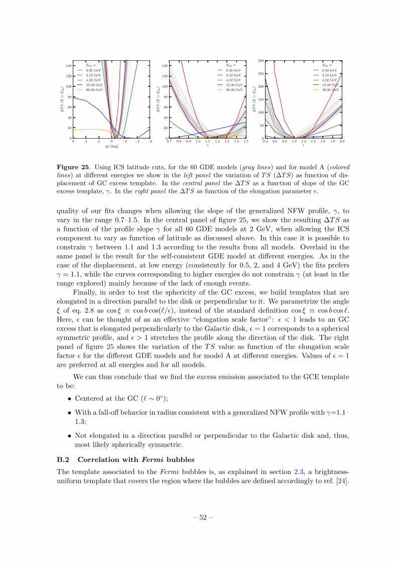
−6−4−20246

∆` [deg]

0

20

40

60

80

100

120

140

∆TS

(E>E

th)

Eth =

0.50 GeV

2.12 GeV

4.32 GeV

12.40 GeV

39.36 GeV

0.7 0.8 0.9 1.0 1.1 1.2 1.3 1.4 1.5γ

0

20

40

60

80

100

120

140

∆TS

(E>E

th)

Eth =

0.50 GeV

2.12 GeV

4.32 GeV

12.40 GeV

39.36 GeV

0.4 0.6 0.8 1.0 1.2 1.4 1.6 1.8 2.0ε

0

50

100

150

200

250

300

∆TS

(E>E

th)

Eth =

0.50 GeV

2.12 GeV

4.32 GeV

12.40 GeV

39.36 GeV

Figure 25. Using ICS latitude cuts, for the 60 GDE models (gray lines) and for model A (coloredlines) at different energies we show in the left panel the variation of TS (∆TS) as function of dis-placement of GC excess template. In the central panel the ∆TS as a function of slope of the GCexcess template, γ. In the right panel the ∆TS as function of the elongation parameter ε.

quality of our fits changes when allowing the slope of the generalized NFW profile, γ, tovary in the range 0.7–1.5. In the central panel of figure 25, we show the resulting ∆TS asa function of the profile slope γ for all 60 GDE models at 2 GeV, when allowing the ICScomponent to vary as function of latitude as discussed above. In this case it is possible toconstrain γ between 1.1 and 1.3 according to the results from all models. Overlaid in thesame panel is the result for the self-consistent GDE model at different energies. As in thecase of the displacement, at low energy (consistently for 0.5, 2, and 4 GeV) the fits prefersγ = 1.1, while the curves corresponding to higher energies do not constrain γ (at least in therange explored) mainly because of the lack of enough events.

Finally, in order to test the sphericity of the GC excess, we build templates that areelongated in a direction parallel to the disk or perpendicular to it. We parametrize the angleξ of eq. 2.8 as cos ξ ≡ cos b cos(`/ε), instead of the standard definition cos ξ ≡ cos b cos `.Here, ε can be thought of as an effective “elongation scale factor”: ε < 1 leads to an GCexcess that is elongated perpendicularly to the Galactic disk, ε = 1 corresponds to a sphericalsymmetric profile, and ε > 1 stretches the profile along the direction of the disk. The rightpanel of figure 25 shows the variation of the TS value as function of the elongation scalefactor ε for the different GDE models and for model A at different energies. Values of ε = 1are preferred at all energies and for all models.

We can thus conclude that we find the excess emission associated to the GCE templateto be:

• Centered at the GC (` ∼ 0);

• With a fall-off behavior in radius consistent with a generalized NFW profile with γ=1.1–1.3;

• Not elongated in a direction parallel or perpendicular to the Galactic disk and, thus,most likely spherically symmetric.

B.2 Correlation with Fermi bubbles

The template associated to the Fermi bubbles is, as explained in section 2.3, a brightness-uniform template that covers the region where the bubbles are defined accordingly to ref. [24].

– 52 –

Extended bubble template (60 × 60)

100 101 102

E [GeV]

10-8

10-7

10-6

10-5

E2dN/dE[G

eVcm

−2s−

1sr]

β =0.0

β =0.1

β =0.5

β =1.5

β =2.5

Extended Bubbles

Std Bubbles

Figure 26. Left panel: Extended (shaded area) and standard (blue line, from ref. [24]) Fermi bubblestemplates used in this work. The red square indicates our ROI. Right panel: Spectrum of GC excesswhen a latitude-dependent bubbles template is included in the fit (results are given for model A).

Latest studies of the Fermi bubbles reanalyzed this region and the emission associated to it[83]. The LAT Collaboration analysis cuts the disk at |b| > 10. Nevertheless, it is likelythat the region of the bubbles extends down to the GC, also in the light of the possibleastrophysical processes that have been attempted to explain this yet unknown emission,e.g. emission of a jet from the central black hole, wind from SN explosion close to the GC, 1st

or 2nd order Fermi acceleration of CR electrons [143–147]. Therefore we consider also a newdefinition of the Fermi bubbles edges28, that extends the bubbles down to the GC. This newregion is displayed in figure 26, left panel, together with the contour of the bubbles region asdefined in ref. [24]. The spectrum associated with the GCE template when the “extended”bubbles template is adopted is displayed in figure 26 (right panel). The new bubbles templateis consistent with the “standard” one – i.e. used as standard working hypothesis – at lowenergies, E ≤ 5 GeV, while it differs at high energies of about 30% at 100 GeV.

We then investigate the possibility that part of the emission absorbed by the GCEtemplate, in particular the high energy end of the spectrum in figure 14, might be corre-lated spatially with the Fermi bubbles. To this end, we adopt an additional template forthe bubbles (built from the new extended bubbles template and in addition to this one),allowing its intensity to be dependent on the latitude ∝ |b|−β, with β < 1 or β > 1. Theemission absorbed by the GCE template when adding a latitude dependent template for theFermi bubbles is shown in figure 26 for different values of the index β. By comparing theTS values of the different templates, it emerges that the fit prefers a template with a verymild latitude dependence, β = 0.1, as well as β = 0 and the extended bubbles template.The standard template adopted in the analysis is only slightly worse than the best-fit one(∆TS = 32), while β ≥ 0.5 is highly disfavored by the fit (∆TS ≥ O(100)). This means thatthe GCE template does not lose too much power when using the latitude-dependent bub-bles template, thus confirming the robustness of our results derived under the assumption ofuniform-brightness template.

28Meng Su, Private Communication.

– 53 –

C Systematic uncertainties

C.1 An analytical model for the empirical model uncertainty

In subsection 4.2 we estimated the model uncertainties from a fit to 22 test regions alongthe Galactic disk. The resulting fluctuations where shown in figure 12 in terms of mean andstandard deviation (left panel), as well decomposed into their principal components (rightpanel). As can be seen from this plot, the first three principal components are sizeableand larger than or comparable to the statistical error, and appear to have a relatively welldefined functional dependence on energy. We will show here that this functional dependenceis actually expected as the result of uncertainties in the normalization and slope of the mainbackground components ICS and π0+Bremss, and can be well fitted with a simple model.

We will start by assuming that the true background flux associated with component kin a given ROI is related to the measured background flux as determined by our templateanalysis by

dN truek

dE= (1 + αk)

(E

Eref

)γk dNk

dE, (C.1)

where, αk and γk are parameters that account for small corrections in the normalization andslope of the flux. These two parameters are unknown, but assumed to be normal distributedwith mean zero and standard deviation ∆αk and ∆γk.

29

We further assume that any mis-modeling of the background will be absorbed by theGCE template, hence

dN trueGCE

dE=

(1−

∑k

(αk − γk ln

E

Eref

))dNGCE

dE, (C.2)

where we neglect second and higher order terms in αk and γk. If only a fraction of mis-modeling is absorbed by the GCE template, this can be accounted for by a rescaling of ∆αkand ∆γk.

The above uncertainty in the GCE spectrum corresponds to a correlation matrix withthe simple form

Σij,mod '∑k

(∆α2

k + ∆γ2k ln

EiEref

lnEjEref

)dNk

dEi

dNk

dEj. (C.3)

This is true as long as the background variations can be modeled as a multivariate normaldistribution, which requires here roughly ∆αk . 0.3 and ∆γk . 0.1, which we will find to bethe case in the present situation.

The background fluxes are derived from the data in our baseline ROI. We will onlytake into account the dominant π0+Bremss and ICS components, and parametrize themanalytically in the simple approximate form

dNπ0+B

dE= 1.0× 10−5 x−2

√x1.2 + x−0.4

GeV−1 cm−2 s−1 sr−1 (C.4)

29Since the errors that we will discuss are typically very small, a more precise modeling of these uncertaintiesin terms of a e.g. log-normal distribution is not of relevance here.

– 54 –

20 30 40 50 60 70 80 90

mχ [GeV]

0.5

1.0

1.5

2.0

2.5

3.0

3.5

4.0

4.5〈σ

v〉

[cm

3s−

1]

×10−26

standard result, model F

w/o method systematics

modeled model systematics

standard result, 60 GDE models

100 101

Ecut [GeV]

−2.0

−1.5

−1.0

−0.5

0.0

0.5

1.0

1.5

2.0

2.5

Spec

tralin

dex

,γ

standard result, model F

E > 600MeV

E < 10GeV

standard result, 60 GDE models

Figure 27. Left panel: Like left panel of figure 18 for bb final states (black contours, based onmodel F), but showing in addition the effect of modeling the background model systematics (lightpink contour), of neglecting the method systematics (light blue contour), and the ±1σ errors that oneobtains for all of the 60 GDE (gray crosses). Right panel: Like right panel of figure 20, but showingin addition the results in the case of restricted energy ranges in the fit (light blue and red curves; only68% CL contours for clarity), and using the 60 GDE models instead (gray crosses).

anddNICS

dE= 4.0× 10−6x−2.3 GeV−1 cm−2 s−1 sr−1 , (C.5)

where x ≡ E/1 GeV. This parametrization is sufficiently accurate for the present purpose.As pivot point for the variations we adopt Eref = 3 GeV, which is again not critical.

We then perform a simple χ2 fit to the three principal components shown in figure 12,giving equal weight to every energy bin and all three components. As a result, we find thebest-fit values ∆απ0+B ' 0.031, ∆γπ0+B . 10−4, ∆αICS ' 0.025 and ∆γICS ' 0.0093. Thecorresponding model predictions are again shown in figure 12, and provide overall a gooddescription of the observed fluctuations.

Taking the above results at face value and referring to fluxes averaged over our baselineROI as e.g. shown in figure 8, the impact of typical mis-modelling of the ICS or π0+Bremsscomponents as observed along the Galactic plane is expected to affect the GCE spectrumonly at the level of a few percent of the background components. Yet, since the backgroundare one order of magnitude stronger, this effect can be still sizeable. In fact, it constitutesone of the major uncertainties when discussing spectral and morphological properties of theGCE excess.

C.2 Various method uncertainties

In figure 27 we show how our results are affected by the most critical analysis choices. In theleft panel, we show a fit to the flux in figure 14 with a bb spectrum. We compare the resultsthat we find for our baseline analysis choices with the results obtained when neglecting the

– 55 –

method uncertainty (cf. figure 13), or when adopting one of the other 59 GDE scenarios tomodel the backgrounds. We find that our results are largely consistent; outliers correspondto GDE models which give a particularly bad TS value.

In the right panel, we show how the fit of a power-law with exponential cutoff is affectedby various analysis choices (cf. figure 20). We show the contours that we obtain whenexcluding data below 600 MeV or above 10 GeV (only 68% CL contours for clarity), as wellas the results obtained when using one of the other 59 GDE models. Again, our resultsremain consistent. Note that excluding data above 10 GeV has the effect of lowering thevalue of the spectral index γ. This can be understood by realizing that the power-law likebehaviour of the GCE (see figure 14) at energies above 10 GeV prefers a larger subtractionof a smooth background (encoded in the correlated model uncertainties, see appendix. C.1)when fitted with an exponential cutoff. This subtraction necessarily affects the flux below 1GeV and makes the spectrum harder.

D Miscellaneous

In figure 28, we show the spectra of the individual background components, as observedin each of the ten segments, for all 60 GDE models. We observe only small variations inthe main GDE components, with the largest variations at low energies in the subdominantFermi bubbles and the isotropic emissions. For reference, we also show the GC excessspectrum for one of the GDE models (model F); the envelope for all other models is shownin figure 16.

– 56 –

10−8

10−7

10−6

10−5

10−4

I II

10−8

10−7

10−6

10−5

10−4

E2dN/dE

[GeV/cm

ssr

]

III IV

10−8

10−7

10−6

10−5

10−4

V VI

10−8

10−7

10−6

10−5

10−4

E2dN/dE

[GeV/cm

ssr

]

VII VIII

100 101 102

E [GeV]

10−8

10−7

10−6

10−5

10−4

IX

100 101 102

E [GeV]

X

Figure 28. Energy spectra of the different background components (π0+Bremss, ICS, the isotropic,bubbles, PSCs) in the template fit, for all 60 GDE models, averaged over the segments shown infigure 15. The color coding is the same as in figure 8. The black points show the results for the GCexcess for model F, as in figure 16.

– 57 –

References

[1] PAMELA Collaboration, S. Orsi, PAMELA: A payload for antimatter matter explorationand light nuclei astrophysics, Nucl. Instrum. Meth. A580 (2007) 880–883.

[2] PAMELA Collaboration, P. Carlson, PAMELA science, Int. J. Mod. Phys. A20 (2005)6731–6734.

[3] www.ams02.org.

[4] N. Gehrels and P. Michelson, GLAST: the next-generation high energy gamma-ray astronomymission, Astroparticle Physics 11 (June, 1999) 277–282.

[5] R. Rando and f. t. F. L. Collaboration, Post-launch performance of the Fermi Large AreaTelescope, arXiv:0907.0626.

[6] WMAP Collaboration, C. Bennett et. al., Nine-Year Wilkinson Microwave Anisotropy Probe(WMAP) Observations: Final Maps and Results, Astrophys.J.Suppl. 208 (2013) 20,[arXiv:1212.5225].

[7] Planck Collaboration Collaboration, J. Tauber et. al., The Scientific programme of Planck,astro-ph/0604069.

[8] K. A. Eriksen, J. P. Hughes, C. Badenes, R. Fesen, P. Ghavamian, et. al., Evidence ForParticle Acceleration to the Knee of the Cosmic Ray Spectrum in Tycho’s SupernovaRemnant, arXiv:1101.1454.

[9] C. Winkler, T.-L. Courvoisier, G. Di Cocco, N. Gehrels, A. Gimenez, et. al., The INTEGRALmission, Astron.Astrophys. 411 (2003) L1–L6.

[10] MAGIC Collaboration Collaboration, J. Albert et. al., Observation of gamma-rays fromthe galactic center with the magic telescope, Astrophys.J. 638 (2006) L101–L104,[astro-ph/0512469].

[11] H.E.S.S. Collaboration Collaboration, F. Aharonian et. al., A New population of very highenergy gamma-ray sources in the Milky Way, Science 307 (2005) 1938–1942,[astro-ph/0504380].

[12] VERITAS Collaboration Collaboration, V. Acciari et. al., Observation of Extended VHEEmission from the Supernova Remnant IC 443 with VERITAS, Astrophys.J. 698 (2009)L133–L137, [arXiv:0905.3291].

[13] IceCube Collaboration Collaboration, M. Aartsen et. al., Observation of High-EnergyAstrophysical Neutrinos in Three Years of IceCube Data, arXiv:1405.5303.

[14] Q. Yuan, S. Liu, Z. Fan, X. Bi, and C. L. Fryer, Modeling the Multi-Wavelength Emission ofShell-Type Supernova Remnant RX J1713.7-3946, Astrophys.J. 735 (2011) 120,[arXiv:1011.0145].

[15] T. Tanaka, A. Allafort, J. Ballet, S. Funk, F. Giordano, et. al., Gamma-Ray Observations ofthe Supernova Remnant RX J0852.0-4622 with the Fermi LAT, Astrophys.J. 740 (2011) L51,[arXiv:1109.4658].

[16] D. Castro, P. Slane, D. C. Ellison, and D. J. Patnaude, Fermi-LAT Observations and ABroadband Study of Supernova Remnant CTB 109, Astrophys.J. 756 (2012) 88,[arXiv:1207.1432].

[17] E. Berezhko, L. Ksenofontov, and H. Voelk, Nonthermal emission of supernova remnant SN1006 revisited: theoretical model and the H.E.S.S. results, Astrophys.J. 759 (2012) 12,[arXiv:1209.2789].

[18] D. Castro, P. Slane, A. Carlton, and E. Figueroa-Feliciano, Fermi-LAT Observations ofSupernova Remnants Interacting with Molecular Clouds: W41, MSH 17-39, and G337.7-0.1,

– 58 –

Astrophys.J. 774 (2013) 36, [arXiv:1305.3623].

[19] L. Saha, T. Ergin, P. Majumdar, M. Bozkurt, and E. Ercan, Origin of gamma-ray emission inthe shell of Cassiopeia A, arXiv:1401.5626.

[20] M. Cardillo, M. Tavani, A. Giuliani, S. Yoshiike, H. Sano, et. al., The Supernova RemnantW44: confirmations and challenges for cosmic-ray acceleration, arXiv:1403.1250.

[21] T. Fukuda, S. Yoshiike, H. Sano, K. Torii, H. Yamamoto, et. al., Interstellar protons in theTeV γ-ray SNR HESS J1731-347: Possible evidence for the coexistence of hadronic andleptonic γ-rays, Astrophys.J. 788 (2014) 94, [arXiv:1405.2599].

[22] The H. E. S. S. Collaboration, Fermi-LAT Collaboration Collaboration,A. Abramowski et. al., Probing the gamma-ray emission from HESS J1834-087 usingH.E.S.S. and Fermi LAT observations, arXiv:1407.0862.

[23] G. Dobler, D. P. Finkbeiner, I. Cholis, T. R. Slatyer, and N. Weiner, The Fermi Haze: AGamma-Ray Counterpart to the Microwave Haze, Astrophys.J. 717 (2010) 825–842,[arXiv:0910.4583].

[24] M. Su, T. R. Slatyer, and D. P. Finkbeiner, Giant Gamma-ray Bubbles from Fermi-LAT: AGNActivity or Bipolar Galactic Wind?, Astrophys. J. 724 (2010) 1044–1082, [arXiv:1005.5480].

[25] D. P. Finkbeiner, Microwave ism emission observed by wmap, Astrophys.J. 614 (2004)186–193, [astro-ph/0311547].

[26] G. Dobler and D. P. Finkbeiner, Extended Anomalous Foreground Emission in the WMAP3-Year Data, Astrophys.J. 680 (2008) 1222–1234, [arXiv:0712.1038].

[27] Planck Collaboration Collaboration, P. Ade et. al., Planck Intermediate Results. IX.Detection of the Galactic haze with Planck, arXiv:1208.5483.

[28] Fermi-LAT Collaboration Collaboration, The Fermi-LAT high-latitude Survey: SourceCount Distributions and the Origin of the Extragalactic Diffuse Background, Astrophys.J. 720(2010) 435–453, [arXiv:1003.0895].

[29] M. Ajello, R. Romani, D. Gasparrini, M. Shaw, J. Bolmer, et. al., The Cosmic Evolution ofFermi BL Lacertae Objects, Astrophys.J. 780 (2014) 73, [arXiv:1310.0006].

[30] Fermi LAT Collaboration Collaboration, A. Abdo, Detection of Gamma-Ray Emissionfrom the Starburst Galaxies M82 and NGC 253 with the Large Area Telescope on Fermi,Astrophys.J. 709 (2010) L152–L157, [arXiv:0911.5327].

[31] B. C. Lacki, T. A. Thompson, E. Quataert, A. Loeb, and E. Waxman, On The GeV and TeVDetections of the Starburst Galaxies M82 and NGC 253, Astrophys.J. 734 (2011) 107,[arXiv:1003.3257].

[32] Fermi LAT Collaboration Collaboration, M. Ackermann et. al., GeV Observations ofStar-forming Galaxies with Fermi LAT, Astrophys.J. 755 (2012) 164, [arXiv:1206.1346].

[33] Fermi LAT collaboration Collaboration, A. Abdo et. al., The First Fermi Large AreaTelescope Catalog of Gamma-ray Pulsars, Astrophys.J.Suppl. 187 (2010) 460–494,[arXiv:0910.1608].

[34] The Fermi-LAT collaboration Collaboration, A. Abdo et. al., The Second Fermi LargeArea Telescope Catalog of Gamma-ray Pulsars, Astrophys.J.Suppl. 208 (2013) 17,[arXiv:1305.4385].

[35] I. Cholis, D. Hooper, and T. Linden, A New Determination of the Spectra and LuminosityFunction of Gamma-Ray Millisecond Pulsars, arXiv:1407.5583.

[36] Fermi-LAT collaboration Collaboration, A. Abdo et. al., The Spectrum of the IsotropicDiffuse Gamma-Ray Emission Derived From First-Year Fermi Large Area Telescope Data,Phys.Rev.Lett. 104 (2010) 101101, [arXiv:1002.3603].

– 59 –

[37] M. Ackermann, Intensity and origin of the extragalactic gamma-ray background, 2012.

[38] Fermi LAT Collaboration Collaboration, M. Ackermann et. al., Anisotropies in the diffusegamma-ray background measured by the Fermi LAT, Phys.Rev. D85 (2012) 083007,[arXiv:1202.2856].

[39] A. Cuoco, E. Komatsu, and J. Siegal-Gaskins, Joint anisotropy and source count constraintson the contribution of blazars to the diffuse gamma-ray background, Phys.Rev. D86 (2012)063004, [arXiv:1202.5309].

[40] F. W. Stecker and T. M. Venters, Components of the Extragalactic Gamma Ray Background,Astrophys.J. 736 (2011) 40, [arXiv:1012.3678].

[41] R. Makiya, T. Totani, and M. Kobayashi, Contribution from Star-Forming Galaxies to theCosmic Gamma-Ray Background Radiation, Astrophys.J. 728 (2011) 158, [arXiv:1005.1390].

[42] V. Berezinsky, A. Gazizov, M. Kachelriess, and S. Ostapchenko, Restricting UHECRs andcosmogenic neutrinos with Fermi-LAT, Phys.Lett. B695 (2011) 13–18, [arXiv:1003.1496].

[43] M. Ahlers, L. Anchordoqui, M. Gonzalez-Garcia, F. Halzen, and S. Sarkar, GZK Neutrinosafter the Fermi-LAT Diffuse Photon Flux Measurement, Astropart.Phys. 34 (2010) 106–115,[arXiv:1005.2620].

[44] K. Murase, J. F. Beacom, and H. Takami, Gamma-Ray and Neutrino Backgrounds as Probesof the High-Energy Universe: Hints of Cascades, General Constraints, and Implications forTeV Searches, JCAP 1208 (2012) 030, [arXiv:1205.5755].

[45] Planck Collaboration Collaboration, P. Ade et. al., Planck 2013 results. XVI. Cosmologicalparameters, Astron.Astrophys. (2014) [arXiv:1303.5076].

[46] G. Jungman, M. Kamionkowski, and K. Griest, Supersymmetric dark matter, Phys.Rept. 267(1996) 195–373, [hep-ph/9506380].

[47] G. Bertone, D. Hooper, and J. Silk, Particle dark matter: Evidence, candidates andconstraints, Phys.Rept. 405 (2005) 279–390, [hep-ph/0404175].

[48] L. Bergstrom, Dark Matter Evidence, Particle Physics Candidates and Detection Methods,Annalen Phys. 524 (2012) 479–496, [arXiv:1205.4882].

[49] L. Goodenough and D. Hooper, Possible Evidence For Dark Matter Annihilation In TheInner Milky Way From The Fermi Gamma Ray Space Telescope, arXiv:0910.2998.

[50] D. Hooper and L. Goodenough, Dark Matter Annihilation in The Galactic Center As Seen bythe Fermi Gamma Ray Space Telescope, Phys.Lett. B697 (2011) 412–428, [arXiv:1010.2752].

[51] D. Hooper and T. Linden, On The Origin Of The Gamma Rays From The Galactic Center,Phys.Rev. D84 (2011) 123005, [arXiv:1110.0006].

[52] K. N. Abazajian and M. Kaplinghat, Detection of a Gamma-Ray Source in the GalacticCenter Consistent with Extended Emission from Dark Matter Annihilation and ConcentratedAstrophysical Emission, Phys.Rev. D86 (2012) 083511, [arXiv:1207.6047].

[53] O. Macias and C. Gordon, The Contribution of Cosmic Rays Interacting With MolecularClouds to the Galactic Center Gamma-Ray Excess, Phys.Rev. D89 (2014) 063515,[arXiv:1312.6671].

[54] K. N. Abazajian, N. Canac, S. Horiuchi, and M. Kaplinghat, Astrophysical and Dark MatterInterpretations of Extended Gamma Ray Emission from the Galactic Center,arXiv:1402.4090.

[55] T. Daylan, D. P. Finkbeiner, D. Hooper, T. Linden, S. K. N. Portillo, et. al., TheCharacterization of the Gamma-Ray Signal from the Central Milky Way: A Compelling Casefor Annihilating Dark Matter, arXiv:1402.6703.

– 60 –

[56] B. Zhou, Y.-F. Liang, X. Huang, X. Li, Y.-Z. Fan, et. al., GeV excess in the Milky Way:Depending on Diffuse Galactic gamma ray Emission template?, arXiv:1406.6948.

[57] A. Boyarsky, D. Malyshev, and O. Ruchayskiy, A comment on the emission from the GalacticCenter as seen by the Fermi telescope, Phys.Lett. B705 (2011) 165–169, [arXiv:1012.5839].

[58] Fermi-LAT Collaboration Collaboration, Fermi-LAT Observations of the DiffuseGamma-Ray Emission: Implications for Cosmic Rays and the Interstellar Medium,Astrophys.J. 750 (2012) 3, [arXiv:1202.4039].

[59] A. W. Strong, I. V. Moskalenko, and O. Reimer, Diffuse galactic continuum gamma rays. AModel compatible with EGRET data and cosmic-ray measurements, Astrophys.J. 613 (2004)962–976, [astro-ph/0406254].

[60] P. D. Serpico and G. Zaharijas, Optimal angular window for observing Dark Matterannihilation from the Galactic Center region: the case of γ− ray lines, Astropart.Phys. 29(2008) 380–385, [arXiv:0802.3245].

[61] E. Nezri, J. Lavalle, and R. Teyssier, Indirect dark matter searches: towards a consistenttop-bottom approach for studying the gamma-ray signals and associated backgrounds,Phys.Rev. D86 (2012) 063524, [arXiv:1204.4121].

[62] D. Hooper and T. R. Slatyer, Two Emission Mechanisms in the Fermi Bubbles: A PossibleSignal of Annihilating Dark Matter, Phys.Dark Univ. 2 (2013) 118–138, [arXiv:1302.6589].

[63] W.-C. Huang, A. Urbano, and W. Xue, Fermi Bubbles under Dark Matter Scrutiny. Part I:Astrophysical Analysis, arXiv:1307.6862.

[64] K. N. Abazajian, The Consistency of Fermi-LAT Observations of the Galactic Center with aMillisecond Pulsar Population in the Central Stellar Cluster, JCAP 1103 (2011) 010,[arXiv:1011.4275].

[65] C. Gordon and O. Macias, Dark Matter and Pulsar Model Constraints from Galactic CenterFermi-LAT Gamma Ray Observations, Phys.Rev. D88 (2013) 083521, [arXiv:1306.5725].

[66] Q. Yuan and B. Zhang, Millisecond pulsar interpretation of the Galactic center gamma-rayexcess, arXiv:1404.2318.

[67] W. Wang, Z. Jiang, and K. Cheng, Contribution to diffuse gamma-rays in the Galactic Centerregion from unresolved millisecond pulsars, Mon.Not.Roy.Astron.Soc. 358 (2005) 263–269,[astro-ph/0501245].

[68] D. Hooper, I. Cholis, T. Linden, J. Siegal-Gaskins, and T. Slatyer, Millisecond pulsars CannotAccount for the Inner Galaxy’s GeV Excess, Phys.Rev. D88 (2013) 083009,[arXiv:1305.0830].

[69] F. Calore, M. Di Mauro, and F. Donato, Diffuse gamma-ray emission from galacticMillisecond Pulsars, arXiv:1406.2706.

[70] I. Cholis, D. Hooper, and T. Linden, Challenges in Explaining the Galactic CenterGamma-Ray Excess with Millisecond Pulsars, arXiv:1407.5625.

[71] F. Yusef-Zadeh, J. W. Hewitt, M. Wardle, V. Tatischeff, D. A. Roberts, W. Cotton,H. Uchiyama, M. Nobukawa, T. G. Tsuru, C. Heinke, and M. Royster, Interacting CosmicRays with Molecular Clouds: A Bremsstrahlung Origin of Diffuse High-energy Emission fromthe Inner 2deg×1deg of the Galactic Center, Astrophys.J. 762 (Jan., 2013) 33,[arXiv:1206.6882].

[72] T. Linden, E. Lovegrove, and S. Profumo, The Morphology of Hadronic Emission Models forthe Gamma-Ray Source at the Galactic Center, Astrophys.J. 753 (2012) 41,[arXiv:1203.3539].

[73] H.E.S.S. Collaboration Collaboration, F. Aharonian et. al., Discovery of very-high-energy

– 61 –

gamma-rays from the galactic centre ridge, Nature 439 (2006) 695–698, [astro-ph/0603021].

[74] F. Yusef-Zadeh, J. Hewitt, M. Wardle, V. Tatischeff, D. Roberts, et. al., Interacting CosmicRays with Molecular Clouds: A Bremsstrahlung Origin of Diffuse High Energy Emission fromthe Inner 2deg by 1deg of the Galactic Center, Astrophys.J. 762 (2013) 33,[arXiv:1206.6882].

[75] E. Carlson and S. Profumo, Cosmic Ray Protons in the Inner Galaxy and the Galactic CenterGamma-Ray Excess, arXiv:1405.7685.

[76] J. Petrovic, P. D. Serpico, and G. Zaharijas, Galactic Center gamma-ray ”excess” from anactive past of the Galactic Centre?, arXiv:1405.7928.

[77] S. K. N. Portillo and D. P. Finkbeiner, Sharper Fermi LAT Images: instrument responsefunctions for an improved event selection, arXiv:1406.0507.

[78] K. Gorski, E. Hivon, A. Banday, B. Wandelt, F. Hansen, et. al., HEALPix - A Framework forhigh resolution discretization, and fast analysis of data distributed on the sphere, Astrophys.J.622 (2005) 759–771, [astro-ph/0409513].

[79] W. Cash, Parameter estimation in astronomy through application of the likelihood ratio,Astrophys.J. 228 (1979) 939–947.

[80] Fermi LAT Collaboration, A. A. Abdo et. al., Fermi Large Area Telescope Second SourceCatalog, arXiv:1108.1435.

[81] A. Franckowiak and M. D., Spectrum of the fermi bubbles, 2013.

[82] A. W. Strong, I. V. Moskalenko, and O. Reimer, Diffuse continuum gamma-rays from thegalaxy, Astrophys.J. 537 (2000) 763–784, [astro-ph/9811296].

[83] Fermi-LAT Collaboration Collaboration, The Spectrum and Morphology of the FermiBubbles, arXiv:1407.7905.

[84] C. Vera-Ciro, L. V. Sales, A. Helmi, and J. F. Navarro, The shape of dark matter subhalos inthe Aquarius simulations, arXiv:1402.0903.

[85] T. Kamae, N. Karlsson, T. Mizuno, T. Abe, and T. Koi, Parameterization of gamma, e+-and neutrino spectra produced by p p interaction in astronomical environment, Astrophys. J.647 (2006) 692–708, [astro-ph/0605581].

[86] S. R. Kelner, F. A. Aharonian, and V. V. Bugayov, Energy spectra of gamma-rays, electronsand neutrinos produced at proton proton interactions in the very high energy regime, Phys.Rev. D74 (2006) 034018, [astro-ph/0606058].

[87] H. Koch and J. Motz, Bremsstrahlung Cross-Section Formulas and Related Data,Rev.Mod.Phys. 31 (1959) 920–955.

[88] R. J. Gould, High-Energy Bremsstrahlung in Collisions of Electrons with One- andTwo-Electron Atoms, Physical Review 185 (Sept., 1969) 72–79.

[89] G. Blumenthal and R. Gould, Bremsstrahlung, synchrotron radiation, and compton scatteringof high-energy electrons traversing dilute gases, Rev.Mod.Phys. 42 (1970) 237–270.

[90] F. C. Jones, Calculated Spectrum of Inverse-Compton-Scattered Photons, Phys.Rev. 167(1968) 1159–1169.

[91] R. Trotta, G. Johannesson, I. Moskalenko, T. Porter, R. R. de Austri, et. al., Constraints oncosmic-ray propagation models from a global Bayesian analysis, Astrophys.J. 729 (2011) 106,[arXiv:1011.0037].

[92] C. Evoli, D. Gaggero, D. Grasso, and L. Maccione, Cosmic-Ray Nuclei, Antiprotons andGamma-rays in the Galaxy: a New Diffusion Model, JCAP 0810 (2008) 018,[arXiv:0807.4730].

– 62 –

[93] I. Cholis and D. Hooper, Constraining the origin of the rising cosmic ray positron fractionwith the boron-to-carbon ratio, Phys.Rev. D89 (2014), no. 4 043013, [arXiv:1312.2952].

[94] I. Cholis, M. Tavakoli, C. Evoli, L. Maccione, and P. Ullio, Diffuse Galactic Gamma Rays atintermediate and high latitudes. I. Constraints on the ISM properties, JCAP 1205 (2012) 004,[arXiv:1106.5073].

[95] A. Hryczuk, I. Cholis, R. Iengo, M. Tavakoli, and P. Ullio, Indirect Detection Analysis: WinoDark Matter Case Study, arXiv:1401.6212.

[96] C. Evoli, I. Cholis, D. Grasso, L. Maccione, and P. Ullio, Antiprotons from dark matterannihilation in the Galaxy: astrophysical uncertainties, Phys.Rev. D85 (2012) 123511,[arXiv:1108.0664].

[97] M. Cirelli and G. Giesen, Antiprotons from Dark Matter: Current constraints and futuresensitivities, JCAP 1304 (2013) 015, [arXiv:1301.7079].

[98] M. Cirelli, D. Gaggero, G. Giesen, M. Taoso, and A. Urbano, Antiproton constraints on theGeV gamma-ray excess: a comprehensive analysis, arXiv:1407.2173.

[99] I. Cholis and D. Hooper, Dark Matter and Pulsar Origins of the Rising Cosmic Ray PositronFraction in Light of New Data From AMS, Phys.Rev. D88 (2013) 023013, [arXiv:1304.1840].

[100] M. Tavakoli, I. Cholis, C. Evoli, and P. Ullio, Constraints on dark matter annihilations fromdiffuse gamma-ray emission in the Galaxy, JCAP 1401 (2014) 017, [arXiv:1308.4135].

[101] H. Nakanishi and Y. Sofue, Three-dimensional distribution of the ISM in the Milky WayGalaxy: 1. The HI disk, Publ.Astron.Soc.Jap. 55 (2003) 191, [astro-ph/0304338].

[102] M. Tavakoli, Three Dimensional Distribution of Atomic Hydrogen in the Milky Way,arXiv:1207.6150.

[103] M. Pohl, P. Englmaier, and N. Bissantz, 3D Distribution of Molecular Gas in the BarredMilky Way, Astrophys.J. 677 (2008) 283–291, [arXiv:0712.4264].

[104] G. Dobler, I. Cholis, and N. Weiner, The Fermi Gamma-Ray Haze from Dark MatterAnnihilations and Anisotropic Diffusion, Astrophys.J. 741 (2011) 25, [arXiv:1102.5095].

[105] D. Gaggero, L. Maccione, G. Di Bernardo, C. Evoli, and D. Grasso, Three-Dimensional Modelof Cosmic-Ray Lepton Propagation Reproduces Data from the Alpha Magnetic Spectrometer onthe International Space Station, Phys.Rev.Lett. 111 (2013), no. 2 021102, [arXiv:1304.6718].

[106] A. W. Strong, I. V. Moskalenko, and V. S. Ptuskin, Cosmic-ray propagation and interactionsin the Galaxy, Ann.Rev.Nucl.Part.Sci. 57 (2007) 285–327, [astro-ph/0701517].

[107] http://galprop.stanford.edu/.

[108] A. W. Strong, I. V. Moskalenko, T. A. Porter, n. J ohannesso, E. Orlando, D. W. Digel, andA. E. Vladimirov, Galprop version 54: Explanatory supplement, 2011.

[109] A. Strong, I. Moskalenko, O. Reimer, S. Digel, and R. Diehl, The distribution of cosmic-raysources in the galaxy, gamma-rays, and the gradient in the co-to-h2 relation,Astron.Astrophys. 422 (2004) L47–L50, [astro-ph/0405275].

[110] T. A. Porter, I. V. Moskalenko, A. W. Strong, E. Orlando, and L. Bouchet, Inverse ComptonOrigin of the Hard X-Ray and Soft Gamma-Ray Emission from the Galactic Ridge,Astrophys.J. 682 (2008) 400–407, [arXiv:0804.1774].

[111] R. M. Crocker, D. Jones, F. Melia, J. Ott, and R. J. Protheroe, A lower limit of 50 microgaussfor the magnetic field near the Galactic Centre, Nature 468 (2010) 65, [arXiv:1001.1275].

[112] G. L. Case and D. Bhattacharya, A new sigma-d relation and its application to the galacticsupernova remnant distribution, Astrophys.J. 504 (1998) 761, [astro-ph/9807162].

[113] D. Lorimer, A. Faulkner, A. Lyne, R. Manchester, M. Kramer, et. al., The Parkes multibeam

– 63 –

pulsar survey: VI. Discovery and timing of 142 pulsars and a Galactic population analysis,Mon.Not.Roy.Astron.Soc. 372 (2006) 777–800, [astro-ph/0607640].

[114] I. Yusifov and I. Kucuk, Revisiting the radial distribution of pulsars in the galaxy,Astron.Astrophys. 422 (2004) 545–553, [astro-ph/0405559].

[115] L. Bronfman, S. Casassus, J. May, and L. Nyman, The radial distribution of ob star formationin the galaxy, astro-ph/0006104.

[116] I. A. Grenier, J.-M. Casandjian, and R. Terrier, Unveiling Extensive Clouds of Dark Gas inthe Solar Neighborhood, Science 307 (Feb., 2005) 1292–1295.

[117] D. J. Schlegel, D. P. Finkbeiner, and M. Davis, Maps of dust IR emission for use in estimationof reddening and CMBR foregrounds, Astrophys.J. 500 (1998) 525, [astro-ph/9710327].

[118] R. Jansson, G. R. Farrar, A. H. Waelkens, and T. A. Ensslin, Constraining models of the largescale Galactic magnetic field with WMAP5 polarization data and extragalactic RotationMeasure sources, JCAP 0907 (2009) 021, [arXiv:0905.2228].

[119] T. Dame, D. Hartmann, and P. Thaddeus, The Milky Way in molecular clouds: A Newcomplete co survey, Astrophys.J. 547 (2001) 792–813, [astro-ph/0009217].

[120] S. Levshakov, C. Henkel, D. Reimers, M. Wang, R. Mao, et. al., Star-forming regions of theAquila rift cloud complex. I. NH3 tracers of dense molecular cores, Astron.Astrophys. 553(2013) A58, [arXiv:1303.2052].

[121] J. Knude, 2mass/Hipparcos Extinctions and Distances in the Serpens - Aquila Region.IV.Error Propagation. Individual stars and mean values, arXiv:1103.0455.

[122] T. P. Robitaille and B. A. Whitney, The present-day star formation rate of the Milky-Waydetermined from Spitzer detected young stellar objects, Astrophys.J. 710 (2010) L11–L15,[arXiv:1001.3672].

[123] P. Gondolo, J. Edsjo, P. Ullio, L. Bergstrom, M. Schelke, et. al., DarkSUSY: Computingsupersymmetric dark matter properties numerically, JCAP 0407 (2004) 008,[astro-ph/0406204].

[124] R. Voss and M. Gilfanov, A study of the population of LMXBs in the bulge of M31,Astron.Astrophys. (2006) [astro-ph/0610649].

[125] K. N. Abazajian and M. Kaplinghat, Detection of a gamma-ray source in the Galactic Centerconsistent with extended emission from dark matter annihilation and concentratedastrophysical emission, Phys.Rev. D 86 (Oct., 2012) 083511, [arXiv:1207.6047].

[126] T. Bringmann, M. Vollmann, and C. Weniger, Updated cosmic-ray and radio constraints onlight dark matter: Implications for the GeV gamma-ray excess at the Galactic center,arXiv:1406.6027.

[127] Fermi-LAT Collaboration Collaboration, M. Ackermann et. al., Dark Matter Constraintsfrom Observations of 25 Milky Way Satellite Galaxies with the Fermi Large Area Telescope,Phys.Rev. D89 (2014) 042001, [arXiv:1310.0828].

[128] I. Cholis and P. Salucci, Extracting limits on Dark Matter annihilation from gamma-rayobservations towards dwarf spheroidal galaxies, Phys.Rev. D86 (2012) 023528,[arXiv:1203.2954].

[129] A. Geringer-Sameth and S. M. Koushiappas, Exclusion of canonical WIMPs by the jointanalysis of Milky Way dwarfs with Fermi, Phys.Rev.Lett. 107 (2011) 241303,[arXiv:1108.2914].

[130] F. Donato, D. Maurin, P. Brun, T. Delahaye, and P. Salati, Constraints on WIMP DarkMatter from the High Energy PAMELA p/p data, Phys. Rev. Lett. 102 (2009) 071301,[arXiv:0810.5292].

– 64 –

[131] I. Cholis, New Constraints from PAMELA anti-proton data on Annihilating and DecayingDark Matter, JCAP 1109 (2011) 007, [arXiv:1007.1160].

[132] L. Bergstrom, T. Bringmann, I. Cholis, D. Hooper, and C. Weniger, New limits on darkmatter annihilation from AMS cosmic ray positron data, Phys.Rev.Lett. 111 (2013) 171101,[arXiv:1306.3983].

[133] A. Ibarra, A. S. Lamperstorfer, and J. Silk, Dark matter annihilations and decays after theAMS-02 positron measurements, Phys.Rev. D89 (2014) 063539, [arXiv:1309.2570].

[134] I. Cholis, D. Hooper, and T. Linden, A Critical Reevaluation of Radio Constraints onAnnihilating Dark Matter, arXiv:1408.6224.

[135] S. Galli, F. Iocco, G. Bertone, and A. Melchiorri, CMB constraints on Dark Matter modelswith large annihilation cross-section, Phys.Rev. D80 (2009) 023505, [arXiv:0905.0003].

[136] T. R. Slatyer, N. Padmanabhan, and D. P. Finkbeiner, CMB Constraints on WIMPAnnihilation: Energy Absorption During the Recombination Epoch, Phys.Rev. D80 (2009)043526, [arXiv:0906.1197].

[137] S. Galli, F. Iocco, G. Bertone, and A. Melchiorri, Updated CMB constraints on Dark Matterannihilation cross-sections, Phys.Rev. D84 (2011) 027302, [arXiv:1106.1528].

[138] C. Evoli, S. Pandolfi, and A. Ferrara, CMB constraints on light dark matter candidates,arXiv:1210.6845.

[139] L. Lopez-Honorez, O. Mena, S. Palomares-Ruiz, and A. C. Vincent, Constraints on darkmatter annihilation from CMB observationsbefore Planck, JCAP 1307 (2013) 046,[arXiv:1303.5094].

[140] D. Hooper and T. Linden, Origin of the gamma rays from the Galactic Center, Phys.Rev. D84 (Dec., 2011) 123005, [arXiv:1110.0006].

[141] E. Jones, T. Oliphant, P. Peterson, et. al., SciPy: Open source scientific tools for Python,2001.

[142] F. Perez and B. E. Granger, IPython: a System for Interactive Scientific Computing, Comput.Sci. Eng. 9 (2007), no. 3 21–29.

[143] F. Guo and W. G. Mathews, The Fermi Bubbles. I. Possible Evidence for Recent AGN JetActivity in the Galaxy, Astrophys.J. 756 (2012) 181, [arXiv:1103.0055].

[144] F. Guo, W. G. Mathews, G. Dobler, and S. P. Oh, The Fermi Bubbles II: The Potential Rolesof Viscosity and Cosmic Ray Diffusion in Jet Models, Astrophys.J. 756 (2012) 182,[arXiv:1110.0834].

[145] R. M. Crocker and F. Aharonian, The Fermi Bubbles: Giant, Multi-Billion-Year-OldReservoirs of Galactic Center Cosmic Rays, Phys.Rev.Lett. 106 (2011) 101102,[arXiv:1008.2658].

[146] K. Cheng, D. Chernyshov, V. Dogiel, C.-M. Ko, and W.-H. Ip, Origin of the Fermi Bubble,Astrophys.J. 731 (2011) L17, [arXiv:1103.1002].

[147] P. Mertsch and S. Sarkar, Fermi gamma-ray ‘bubbles’ from stochastic acceleration of electrons,Phys.Rev.Lett. 107 (2011) 091101, [arXiv:1104.3585].

– 65 –