backpropagation in multilayer perceptronscis.poly.edu/~mleung/cs6673/s09/backpropagation.pdf · the...
TRANSCRIPT

POLYTECHNIC UNIVERSITYDepartment of Computer and Information Science
Backpropagation in MultilayerPerceptrons
K. Ming Leung
Abstract: A training algorithm for multilayer percep-trons known as backpropagation is discussed.
Directory• Table of Contents• Begin Article
Copyright c© 2008 [email protected] Revision Date: March 3, 2008
Table of Contents
1. Introduction
2. Multilayer Perceptron
3. Backpropagation Algorithm
4. Variations of the Basic Backpropagation Algorithm4.1. Modified Target Values4.2. Other Transfer Functions4.3. Momentum4.4. Batch Updating4.5. Variable Learning Rates4.6. Adaptive Slope
5. Multilayer NN as Universal Approximations
Section 1: Introduction 3
1. Introduction
Single-layer networks are capable of solving only linearly separableclassification problems. Researches were aware of this limitation andhave proposed multilayer networks to overcome this. However theywere not able to generalize their training algorithms to these multi-layer networks until the thesis work of Werbos in 1974. Unfortunatelythis work was not known to the neural network community until afterit was rediscovered independently by a number of people in the middle1980s. The training algorithm, now known as backpropagation (BP),is a generalization of the Delta (or LMS) rule for single layer percep-tron to include differentiable transfer function in multilayer networks.BP is currently the most widely used NN.
2. Multilayer Perceptron
We want to consider a rather general NN consisting of L layers (ofcourse not counting the input layer). Let us consider an arbitrarylayer, say `, which has N` neurons X(`)
1 , X(`)2 , . . . , X(`)
N`, each with a
transfer function f (`). Notice that the transfer function may be dif-Toc JJ II J I Back J Doc Doc I
Section 2: Multilayer Perceptron 4
ferent from layer to layer. As in the extended Delta rule, the transferfunction may be given by any differentiable function, but does notneed to be linear. These neurons receive signals from the neurons inthe preceding layer, `− 1. For example, neuron X(`)
j receives a signal
from X(`−1)i with a weight factor w(`)
ij . Therefore we have an N`−1
by N` weight matrix, W(`), whose elements are given by W(`)ij , for
i = 1, 2, . . . , N`−1 and j = 1, 2, . . . , N`. Neuron X(`)j also has a bias
given by b(`)j , and its activation is a(`)j .
To simplify the notation, we will use n(`)j (= yin,j) to denote the
net input into neuron X(`)j . It is given by
n(`)j =
N`−1∑i=1
a(`−1)i w
(`)ij + b
(`)j , j = 1, 2, . . . , N`.
Toc JJ II J I Back J Doc Doc I

Section 2: Multilayer Perceptron 5
X(0)1
X(0)N0
X(1)1
X(1)N1
X(�−1)1
X(�−1)i
X(�−1)N�−1
X(�)1
X(�)j
X(�)N�
X(L−1)1
X(L−1)NL−1
X(L)1
X(L)NL
W(�)ij
a(0)1
a(0)N0
a(L)1
a(L)NL
Figure 1: A general multilayer feedforward neural network.
Toc JJ II J I Back J Doc Doc I
Section 2: Multilayer Perceptron 6
Thus the activation of neuron X(`)j is
a(`)j = f (`)(n(`)
j ) = f (`)(N`−1∑i=1
a(`−1)i w
(`)ij + b
(`)j ).
We can consider the zeroth layer as the input layer. If an inputvector x has N components, then N0 = N and neurons in the inputlayer have activations a(0)
i = xi, i = 1, 2, . . . , N0.Layer L of the network is the output layer. Assuming that the
output vector y has M components, then we must have NL = M .These components are given by yj = a
(L)j , j = 1, 2, . . . ,M .
For any given input vector, the above equations can be used tofind the activation for each neuron for any given set of weights andbiases. In particular the network output vector y can be found. Theremaining question is how to train the network to find a set of weightsand biases in order for it to perform a certain task.
Toc JJ II J I Back J Doc Doc I
Section 3: Backpropagation Algorithm 7
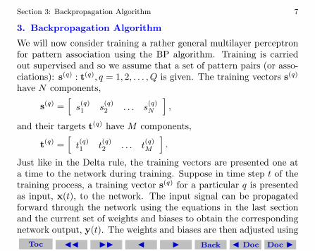
3. Backpropagation Algorithm
We will now consider training a rather general multilayer perceptronfor pattern association using the BP algorithm. Training is carriedout supervised and so we assume that a set of pattern pairs (or asso-ciations): s(q) : t(q), q = 1, 2, . . . , Q is given. The training vectors s(q)
have N components,
s(q) =[s(q)1 s
(q)2 . . . s
(q)N
],
and their targets t(q) have M components,
t(q) =[t(q)1 t
(q)2 . . . t
(q)M
].
Just like in the Delta rule, the training vectors are presented one ata time to the network during training. Suppose in time step t of thetraining process, a training vector s(q) for a particular q is presentedas input, x(t), to the network. The input signal can be propagatedforward through the network using the equations in the last sectionand the current set of weights and biases to obtain the correspondingnetwork output, y(t). The weights and biases are then adjusted using
Toc JJ II J I Back J Doc Doc I

Section 3: Backpropagation Algorithm 8
the steepest descent algorithm to minimize the square of the error forthis training vector:
E = ‖y(t)− t(t)‖2,where t(t) = t(q) is the corresponding target vector for the chosentraining vector s(q).
This square error E is a function of all the weights and biases ofthe entire network since y(t) depends on them. We need to find theset of updating rule for them based on the steepest descent algorithm:
w(`)ij (t+ 1) = w
(`)ij (t)− α ∂E
∂w(`)ij (t)
b(`)j (t+ 1) = b
(`)j (t)− α ∂E
∂b(`)j (t)
,
where α(> 0) is the learning rate.To compute these partial derivatives, we need to understand how
E depends on the weights and biases. First E depends explicitly onthe network output y(t) (the activations of the last layer, a(L)), which
Toc JJ II J I Back J Doc Doc I

Section 3: Backpropagation Algorithm 9
then depends on the net input into the L−th layer, n(L). In turn n(L)
is given by the activations of the preceding layer and the weights andbiases of layer L. The explicit relation is: for brevity, the dependenceon step t is omitted
E = ‖y − t(t)‖2 = ‖a(L) − t(t)‖2 = ‖f (L)(n(L))− t(t)‖2
=
∥∥∥∥∥∥f (L)
NL−1∑i=1
a(L−1)i w
(L)ij + b
(L)j
− t(t)
∥∥∥∥∥∥2
.
It is then easy to compute the partial derivatives of E with respect tothe elements of W(L) and b(L) using the chain rule for differentiation.We have
∂E
∂w(L)ij
=NL∑n=1
∂E
∂n(L)n
∂n(L)n
∂w(L)ij
.
Notice the sum is needed in the above equation for correct applicationof the chain rule. We now define the sensitivity vector for a general
Toc JJ II J I Back J Doc Doc I
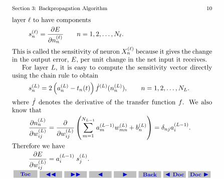
Section 3: Backpropagation Algorithm 10
layer ` to have components
s(`)n =∂E
∂n(`)n
n = 1, 2, . . . , N`.
This is called the sensitivity of neuron X(`)n because it gives the change
in the output error, E, per unit change in the net input it receives.For layer L, it is easy to compute the sensitivity vector directly
using the chain rule to obtain
s(L)n = 2
(a(L)n − tn(t)
)f (L)(n(L)
n ), n = 1, 2, . . . , NL.
where f denotes the derivative of the transfer function f . We alsoknow that
∂n(L)n
∂w(L)ij
=∂
∂w(L)ij
NL−1∑m=1
a(L−1)m w(L)
mn + b(L)n
= δnja(L−1)i .
Therefore we have∂E
∂w(L)ij
= a(L−1)i s
(L)j .
Toc JJ II J I Back J Doc Doc I
Section 3: Backpropagation Algorithm 11
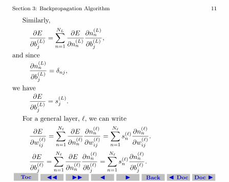
Similarly,
∂E
∂b(L)j
=NL∑n=1
∂E
∂n(L)n
∂n(L)n
∂b(L)j
,
and since
∂n(L)n
∂b(L)j
= δnj ,
we have∂E
∂b(L)j
= s(L)j .
For a general layer, `, we can write
∂E
∂w(`)ij
=N∑n=1
∂E
∂n(`)n
∂n(`)n
∂w(`)ij
=N∑n=1
s(`)n∂n
(`)n
∂w(`)ij
.
∂E
∂b(`)j
=N∑n=1
∂E
∂n(`)n
∂n(`)n
∂b(`)j
=N∑n=1
s(`)n∂n
(`)n
∂b(`)j
.
Toc JJ II J I Back J Doc Doc I
Section 3: Backpropagation Algorithm 12
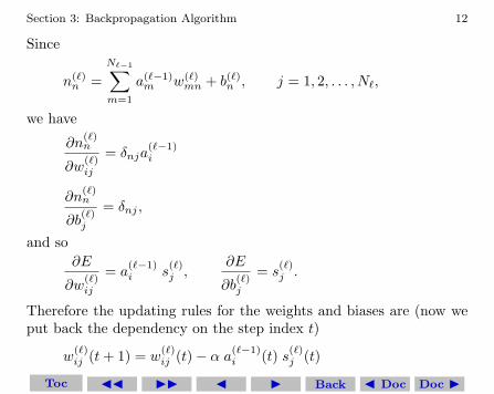
Since
n(`)n =
N`−1∑m=1
a(`−1)m w(`)
mn + b(`)n , j = 1, 2, . . . , N`,
we have
∂n(`)n
∂w(`)ij
= δnja(`−1)i
∂n(`)n
∂b(`)j
= δnj ,
and so∂E
∂w(`)ij
= a(`−1)i s
(`)j ,
∂E
∂b(`)j
= s(`)j .
Therefore the updating rules for the weights and biases are (now weput back the dependency on the step index t)
w(`)ij (t+ 1) = w
(`)ij (t)− α a(`−1)
i (t) s(`)j (t)
Toc JJ II J I Back J Doc Doc I
Section 3: Backpropagation Algorithm 13
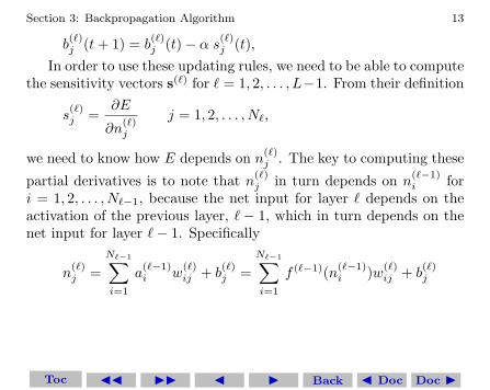
b(`)j (t+ 1) = b
(`)j (t)− α s(`)j (t),
In order to use these updating rules, we need to be able to computethe sensitivity vectors s(`) for ` = 1, 2, . . . , L−1. From their definition
s(`)j =
∂E
∂n(`)j
j = 1, 2, . . . , N`,
we need to know how E depends on n(`)j . The key to computing these
partial derivatives is to note that n(`)j in turn depends on n
(`−1)i for
i = 1, 2, . . . , N`−1, because the net input for layer ` depends on theactivation of the previous layer, ` − 1, which in turn depends on thenet input for layer `− 1. Specifically
n(`)j =
N`−1∑i=1
a(`−1)i w
(`)ij + b
(`)j =
N`−1∑i=1
f (`−1)(n(`−1)i )w(`)
ij + b(`)j
Toc JJ II J I Back J Doc Doc I
Section 3: Backpropagation Algorithm 14
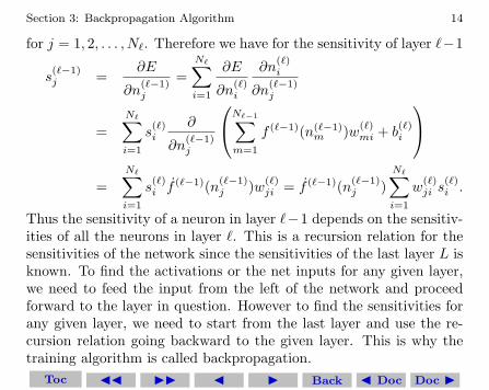
for j = 1, 2, . . . , N`. Therefore we have for the sensitivity of layer `−1
s(`−1)j =
∂E
∂n(`−1)j
=N∑i=1
∂E
∂n(`)i
∂n(`)i
∂n(`−1)j
=N∑i=1
s(`)i
∂
∂n(`−1)j
N`−1∑m=1
f (`−1)(n(`−1)m )w(`)
mi + b(`)i
=
N∑i=1
s(`)i f (`−1)(n(`−1)
j )w(`)ji = f (`−1)(n(`−1)
j )N∑i=1
w(`)ji s
(`)i .
Thus the sensitivity of a neuron in layer `−1 depends on the sensitiv-ities of all the neurons in layer `. This is a recursion relation for thesensitivities of the network since the sensitivities of the last layer L isknown. To find the activations or the net inputs for any given layer,we need to feed the input from the left of the network and proceedforward to the layer in question. However to find the sensitivities forany given layer, we need to start from the last layer and use the re-cursion relation going backward to the given layer. This is why thetraining algorithm is called backpropagation.
Toc JJ II J I Back J Doc Doc I

Section 3: Backpropagation Algorithm 15
In summary, the backpropagation algorithm for training a multi-layer perceptron is
Toc JJ II J I Back J Doc Doc I

Section 3: Backpropagation Algorithm 16
1. Set α. Initialize weights and biases.
2. For step t = 1, 2, . . ., repeat steps a-e until convergence.a Set a(0) = x(t) randomly picked from training set.b For ` = 1, 2, . . . , L, compute
n(`) = a(`−1)W(`) + b(`) a(`) = f (`)(n(`)).
c Compute for n = 1, 2, . . . , NL
s(L)n = 2
(a(L)n − tn(t)
)f (L)(n(L)
n ).
d For ` = L− 1, . . . , 2, 1 and j = 1, 2, . . . , N`, compute
s(`)j = f (`)(n(`)
j )N`+1∑i=1
w(`+1)ji s
(`+1)i .
e For ` = 1, 2, . . . , L, update
w(`)ij (t+ 1) = w
(`)ij (t)− α a(`−1)
i (t) s(`)j (t),
b(`)j (t+ 1) = b
(`)j (t)− α s(`)j (t).
Toc JJ II J I Back J Doc Doc I
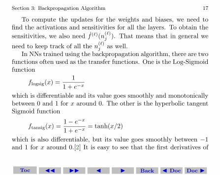
Section 3: Backpropagation Algorithm 17
To compute the updates for the weights and biases, we need tofind the activations and sensitivities for all the layers. To obtain thesensitivities, we also need f (`)(n(`)
j ). That means that in general we
need to keep track of all the n(`)j as well.
In NNs trained using the backpropagation algorithm, there are twofunctions often used as the transfer functions. One is the Log-Sigmoidfunction
flogsig(x) =1
1 + e−x
which is differentiable and its value goes smoothly and monotonicallybetween 0 and 1 for x around 0. The other is the hyperbolic tangentSigmoid function
ftansig(x) =1− e−x1 + e−x
= tanh(x/2)
which is also differentiable, but its value goes smoothly between −1and 1 for x around 0.[2] It is easy to see that the first derivatives of
Toc JJ II J I Back J Doc Doc I
Section 4: Variations of the Basic Backpropagation Algorithm 18
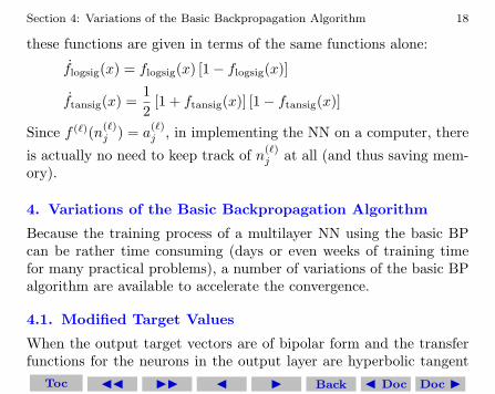
these functions are given in terms of the same functions alone:
flogsig(x) = flogsig(x) [1− flogsig(x)]
ftansig(x) =12
[1 + ftansig(x)] [1− ftansig(x)]
Since f (`)(n(`)j ) = a
(`)j , in implementing the NN on a computer, there
is actually no need to keep track of n(`)j at all (and thus saving mem-
ory).
4. Variations of the Basic Backpropagation Algorithm
Because the training process of a multilayer NN using the basic BPcan be rather time consuming (days or even weeks of training timefor many practical problems), a number of variations of the basic BPalgorithm are available to accelerate the convergence.
4.1. Modified Target Values
When the output target vectors are of bipolar form and the transferfunctions for the neurons in the output layer are hyperbolic tangent
Toc JJ II J I Back J Doc Doc I

Section 4: Variations of the Basic Backpropagation Algorithm 19
Sigmoid functions, since the required output values of ±1 occur atthe asymptotes of the transfer functions, those values can never bereached. The inputs into these neurons need to have extremely largemagnitudes. However this happens only when the weights eventu-ally take on extremely large magnitudes also. Thus the convergenceare typically very slow. The same is true if binary vectors are usedtogether with the binary Sigmoid function.
One easy way out is to consider the net to have learned a particulartraining vector if the computed output values are within a specifiedtolerance of some modified desired values. Good modified values forthe hyperbolic tangent Sigmoid function is ±0.8. Use of modifiedvalues too close to 0 may actually prolong the convergence.
4.2. Other Transfer Functions
The arctangent function is sometimes used as transfer function inBP. It approaches its asymptotic values (saturates) more slowly thanthe hyperbolic tangent Sigmoid function. Scaled so that the function
Toc JJ II J I Back J Doc Doc I
Section 4: Variations of the Basic Backpropagation Algorithm 20
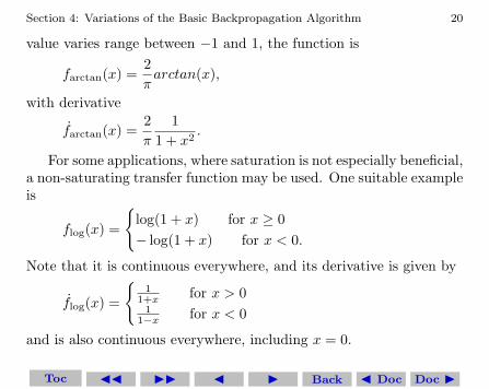
value varies range between −1 and 1, the function is
farctan(x) =2πarctan(x),
with derivative
farctan(x) =2π
11 + x2
.
For some applications, where saturation is not especially beneficial,a non-saturating transfer function may be used. One suitable exampleis
flog(x) =
{log(1 + x) for x ≥ 0− log(1 + x) for x < 0.
Note that it is continuous everywhere, and its derivative is given by
flog(x) =
{1
1+x for x > 01
1−x for x < 0
and is also continuous everywhere, including x = 0.
Toc JJ II J I Back J Doc Doc I

Section 4: Variations of the Basic Backpropagation Algorithm 21
Radial basis functions are also used as transfer functions in BP.These functions have non-negative responses that are localized aroundparticular input values. A common example is the Gaussian function,
fgaussian(x) = exp(−x2)
which is localized around x = 0. Its derivative is
fgaussian(x) = −2x exp(−x2) = −2xfgaussian(x).
4.3. Momentum
Convergence is sometimes faster if a momentum term is added to theweight update formulas. In the simplest form of BP with momentum,the momentum term is proportional to the change in the weights inthe previous step:
∆w(`)ij (t+ 1) = α a
(`−1)i (t) s(`)j (t) + µ∆w(`)
ij (t),
where the momentum parameter µ lies in the range (0 1). Thereforeupdates of the weights proceed in a combination of the current gra-dient direction and that of the previous gradient. Momentum allows
Toc JJ II J I Back J Doc Doc I
Section 4: Variations of the Basic Backpropagation Algorithm 22
the net to make reasonably large weight adjustments as long as thecorrections are in the same general direction for several successive in-put patterns. It also prevents a large response to the error from anyone single training pattern.
4.4. Batch Updating
In some cases it is advantageous to accumulate the weight correctionterms for several patterns (or even an entire epoch if there are not toomany patterns) and make a single weight adjustment for each weightrather than updating the weights after each pattern is presented. Thisprocedure has a smoothing effect on the correction terms somewhatsimilar to the use of momentum.
4.5. Variable Learning Rates
Just like the original Delta rule for a single layer NN, the use ofvariable learning rates may accelerate the convergence. Each weightmay even have its own learning rate. The learning rates may varyadaptively with time as training progress.
Toc JJ II J I Back J Doc Doc I

Section 4: Variations of the Basic Backpropagation Algorithm 23
4.6. Adaptive Slope
An adjustable parameter can be introduced into the transfer func-tion to control the slope of the function. For example instead of thehyperbolic tangent Sigmoid function
ftansig(x) =1− e−x1 + e−x
= tanh(x/2)
we can use the hyperbolic tangent Sigmoid function
ftansig(x) =1− e−σx1 + e−σx
= tanh(σx/2),
where σ(> 0) controls the magnitude of the slope. The larger σ is,the larger is the derivative of the transfer function. Each neuron canhave its own transfer function with a different slope parameter.
Updating formulas for the weights, biases, and slope parameterscan be derived. Although the net input into neuron X(`)
j is still given
Toc JJ II J I Back J Doc Doc I

Section 4: Variations of the Basic Backpropagation Algorithm 24
by
n(`)j =
N`−1∑i=1
a(`−1)i w
(`)ij + b
(`)j , j = 1, 2, . . . , N`,
its activation is now given by
a(`)j = f (`)(σ(`)
j n(`)j ) = f (`)
σ(`)j
N`−1∑i=1
a(`−1)i w
(`)ij + b
(`)j
,
where σ(`)j is the slope parameter for neuron X
(`)j .
The sensitivities for neurons in the output layer are given by
s(L)n = 2
(a(L)n − tn(t)
)f (L)(σ(L)
n n(L)n ), n = 1, 2, . . . , NL.
The sensitivities of all the other layers can then be obtained from thefollowing recursion relation
s(`−1)j = f (`−1)(n(`−1)
j )N∑i=1
w(`)ji s
(`)i σ
(`)i .
Toc JJ II J I Back J Doc Doc I
Section 5: Multilayer NN as Universal Approximations 25
The updating rules for the weights, biases, and slope parametersare given by
∆w(`)ij (t) = −α a(`−1)
i (t) s(`)j (t) σ(`)j (t)
∆b(`)j (t) = −α s(`)j (t) σ(`)j (t),
∆σ(`)j (t) = −α ∂E
∂σ(`)j (t)
= α s(`)j (t) n
(`)j (t).
The slope parameters are typically initialized to 1 unless one hassome ideas of what their proper values are supposed to be. The useof adjustable slopes usually improves the convergence, however at theexpense of slightly more complicated computation per step.
5. Multilayer NN as Universal Approximations
One use of a NN is to approximate a continuous mapping. It can beshown that a feedforward NN with an input layer, a hidden layer, andan output layer can represent any continuous function exactly. Thisis known as the Kolmogorov mapping NN existence theorem.
Toc JJ II J I Back J Doc Doc I

Section 5: Multilayer NN as Universal Approximations 26
With the use of appropriate transfer functions and a sufficientlylarge number of hidden layers, a NN can approximate both a functionand its derivative. This is useful for applications such as a robotlearning smooth movements.
Toc JJ II J I Back J Doc Doc I

Section 5: Multilayer NN as Universal Approximations 27
References
[1] See Chapter 6 in Laurene Fausett, ”Fundamentals of Neural Net-works - Architectures, Algorithms, and Applications”, PrenticeHall, 1994.
[2] The hyperbolic tangent Sigmoid function may be good for inputvectors that have continuous real-values, and the target vectorshave components in the range [−1 1]. We can easily change thisrange to any other finite interval, such as [a b], by defining a newtransfer function
g(x) = γflogsig(x) + η
which is related to flogsig via a linear transformation. Since wewant g = a when flogsig = −1, therefore we have −γ+ η = a. Alsowe want g = b when flogsig = 1 , therefore we have γ + η = b.Solving for a and b gives
η =a+ b
2, γ =
b− a2
.
Toc JJ II J I Back J Doc Doc I

Section 5: Multilayer NN as Universal Approximations 28
Therefore
g(x) =12
((b− a)flogsig(x) + a+ b) .
17
Toc JJ II J I Back J Doc Doc I