MEASUREMENT ERRORS AND BACKTESTING METHODS

Group 2

Value-at-Risk (VaR) is a risk model which predicts the loss that an investment portfolio may experience over a period of time.

  In order to evaluate the quality of the

VAR estimates, the models should always be backtested with appropriate methods.

Backtesting

A technique used to compare the predicted losses from VaR with the actual losses realised at the end of the period of time. 

This identifies instances where VaR has been underestimated, meaning a portfolio has experienced a loss greater or than the original VaR estimate.

The results of the Back Testing can be used to refine the models used for the VaR predictions, making them more accurate and reducing the risk of unexpected losses.

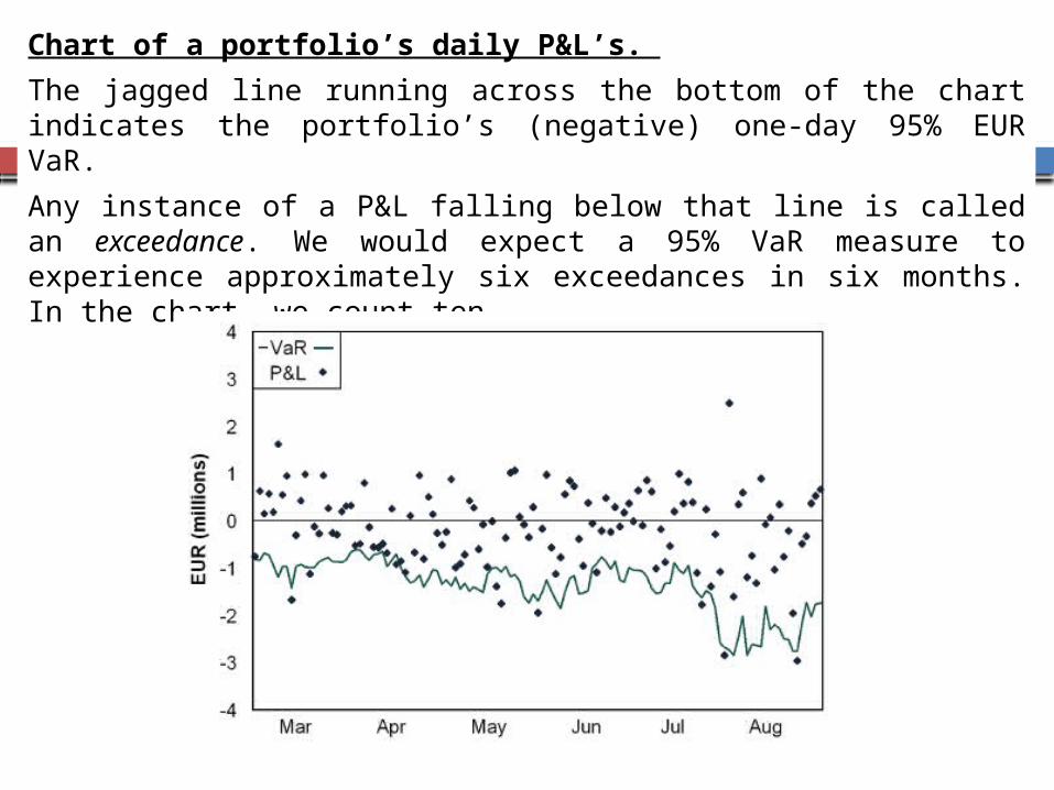
Chart of a portfolio’s daily P&L’s.

The jagged line running across the bottom of the chart indicates the portfolio’s (negative) one-day 95% EUR VaR.

Any instance of a P&L falling below that line is called an exceedance. We would expect a 95% VaR measure to experience approximately six exceedances in six months. In the chart, we count ten.

Key Points of Back Testing Value-at-Risk

1. The following minimum standards apply to calculating capital charge within a model measuring market risk;

2. Data sets should be updated at least once every 3 months

3. VaR must be calculated on a daily basis

4. 99th percentile, one-tailed confidence interval is to be used

5. A 10 day movement in prices should be used as the instant price shock

6. 1 year is classified as a minimum period for “historical” observations

For example, if the confidence level used for calculating daily VaR is 99%, we expect an exception to occur once in every 100 days on average.

In the backtesting process, we could statistically examine whether the frequency of exceptions over some specified time interval is in line with the selected confidence level.

Research to date has focused on VaR measures used by banks. Published backtesting methodologies mostly fall into three categories: Coverage tests – assess whether the frequency

of exceedances is consistent with the quantile of loss a VaR measure is intended to reflect.

Distribution tests – are goodness-of-fit tests applied to the overall loss distributions forecast by complete VaR measures.

Independence tests – assess whether results appear to be independent from one period to the next.

In this respect, an accurate VaR model needs to satisfy the so-called Unconditional Coverage Property.

Unconditional Coverage – refers to the fact that the fraction of overshootings obtained should be in line with the confidence level of VaR.

Failure of unconditional coverage means that the calculated VaR does not measure the risk accurately.

Unconditional Coverage

Denoting the number of exceptions as x and the total number of observations as T:

We may define the failure rate as x/T. In an ideal situation, this rate would reflect the

selected confidence level. For instance, if a confidence level of 99 % is used,

we have a null hypothesis that the frequency of tail losses is equal to p = (1-c) = 1-0.99 = 1%.

Assuming that the model is accurate, the observed failure rate x/T should act as an unbiased measure of p, and thus converge to 1% as sample size is increased.

Each trading outcome either produces a VaR violation exception or not. This sequence of ‘successes and failures’ is commonly known as Bernoulli trial.

The number of exceptions, x ,follows a binomial probability distribution:

By utilizing this binomial distribution we can examine the accuracy of the VaR model.

However, when conducting a statistical backtest that either accepts or rejects a null hypothesis (of the model being ‘good’), there is a tradeoff between two types of errors.

Type I errors occur when we reject the model which is correct, while Type II errors occur when we fail to reject (that is incorrectly accept) the wrong model.

It is clear that in risk management, it can be much more costly to incur in type II errors, and therefore we should impose a high threshold in order to accept the validity of any risk model.

Type I error (rejecting a correct model) probability of committing is 10.8%It describes an accurate model, where p=1%

Type II error (accepting an inaccurate model) probability of committing is 12.8% It describes an inaccurate model where p=3%

Independence Property

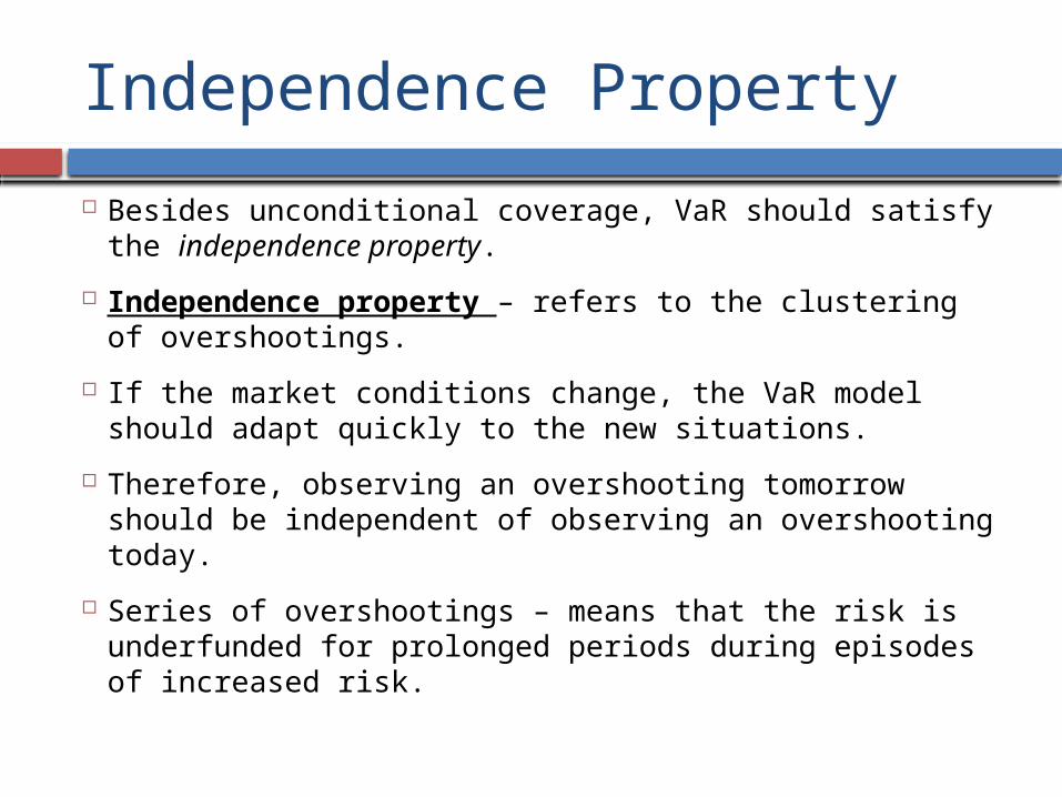
Besides unconditional coverage, VaR should satisfy the independence property.

Independence property – refers to the clustering of overshootings.

If the market conditions change, the VaR model should adapt quickly to the new situations.

Therefore, observing an overshooting tomorrow should be independent of observing an overshooting today.

Series of overshootings – means that the risk is underfunded for prolonged periods during episodes of increased risk.

Independence Property

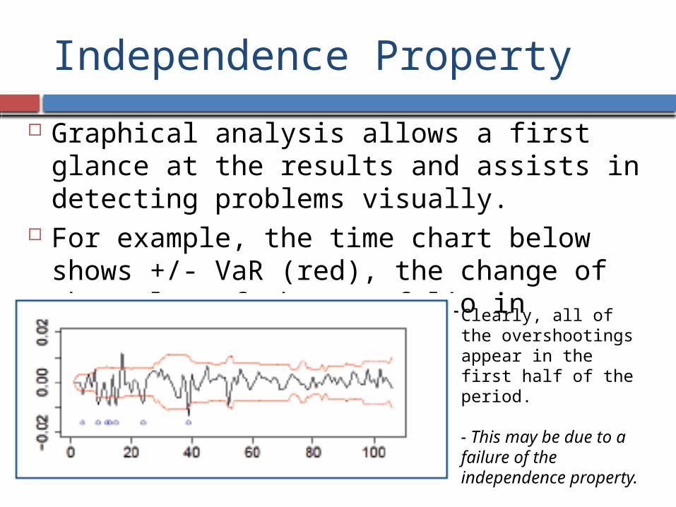
Graphical analysis allows a first glance at the results and assists in detecting problems visually.

For example, the time chart below shows +/- VaR (red), the change of the value of the portfolio in percent (black), and the overshootings (blue).

Clearly, all of the overshootings appear in the first half of the period.

- This may be due to a failure of the independence property.

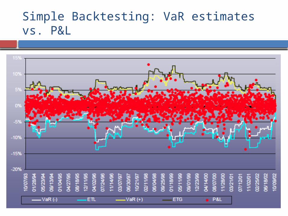
Simple Backtesting: VaR estimates vs. P&L

The simplest backtest consist of counting the number of exceptions (losses larger than estimated VaR) for a given period and comparing to the expected number for the chosen confidence interval.

A more rigorous way to perform the backtesting analysis is to determine the accuracy of the model predicting both the frequency and the size of expected losses.

Backtesting Expected Tail Loss (ETL) or Expected Tail Gain (ETG) numbers can provide an indication of how well the model captures the size of the expected loss (gain) beyond VaR, and therefore can enhance the quality of the backtesting procedure.

Backtesting

- Statistical testing that consist of checking whether actual trading losses are in line with the VAR forecastsIn its simplest form, the backtesting procedure consists of calculating the number or percentage of times that the actual portfolio returns fall outside the VaR estimate, and comparing that number to the confidence level used.

The Basel back-testing framework consists in recording daily exception of the 99% VAR over the last year

Even though capital requirements are based on 10 days VAR, back testing uses a daily interval, which entails more observations

On average, one would expect 1% of 250 or 2.5 instances of exceptions over the last year

Too many exceptions indicate that either the model is understating VAR the Bank is unlucky How to decide ? Statistical inference

On average, the number should be about 2.5 Higher number could happen either because of

Bad Luck or because of a wrong risk model However, it is unlikely that this outcome is due

solely to bad luck

Visualizing VAR : Example

A 1-day VAR of $10mm using a probability of 5% means that there is a 5% chance that the portfolio could lose more than $10mm in the next trading day.

5%

1.645 Std Dev

Possible Profit/Loss-10MM

Test of Frequency of Tail Losses or Kupiec Test

Kupiec’s (1995) test attempts to determine whether the observed frequency of exceptions is consistent with the frequency of expected exceptions according to the VaR model and chosen confidence interval. Under the null hypothesis that the model is “correct”, the number of exceptions follows a binomial distribution.

The probability 1 of experiencing x or more exceptions if the model is correct is given by:

Where x is the number of exceptions, p is the probability of an exception for a given confidence level, and n is the number of trials.

If the estimated probability is above the desired “null” significance level (usually 5% -10%), we accept the model.

If the estimated probability is below the significance level, we reject the model and conclude that it is not correct. We can conduct this test for loss and gain exceptions to determine how well the model predicts the frequency of losses and gains beyond VaR numbers.

Christoffersen’s Independence Test A likelihood ratio test that looks for unusually frequent consecutive exceedances. However, it isn’t defined when there are no

consecutive exceedances at all. In some cases it may be reasonable to simply

accept the null hypothesis when there are no consecutive exceedances. But, not always.

For example, if you backtest a one-day 99% VaR measure with 1,000 days of data, there should be about 10 instances of consecutive exceedances. If there are none, it might be inappropriate to accept the null hypothesis.

Basel Committee “Traffic Light” approach

Market-risk capital multiplier, k is suggested by the Basel Committee in the Capital Accord, which is used to compensate for the possible unreliability of the bank’s VaR calculator.

The exceptions in 250 days is assumed to follow a Bernoulli distribution

The need for VAR model accuracy

If the VAR is systematically “too low”, the model is underestimating the risk and you tend to have too many occasions where the loss in the portfolio exceeds the VAR. This can lead to an increase in the “multiplier” for the capital calculation.

If the VAR is systematically “too high”, the model is over estimating the risk and your regulatory capital charge will be too high

Obtaining Good Historical Data

Poor Data– Even actively traded markets can have “noisy” historical data– Less actively traded markets can pose a significant challenge to finding clean historical data – Historical data can be misleading if a market is maturing over that period

Missing Data– It may be difficult to find historical data in relatively new (e.g., U.K. Asset Backeds) or inactive markets (e.g., inverse I.O.s)

Asynchronous Data– The data for risk factors that are traded against each other (e.g., Mortgages and Treasuries, Futures and Cash Securities, etc.) must reflect simultaneous closes.

Quantitative Standards

Each bank must meet, on a daily basis, a capital requirement expressed as the higher of

(i) its previous day’s value-at-risk number measured according to the parameters specified in this section and

(ii) an average of the daily value-at-risk measures on each of the preceding sixty business days, multiplied by a multiplication factor

multiplication factor will be set by supervisory authorities on the basis of their assessment of the quality of the banks risk management system, subject to an absolute minimum of 3.

Banks using models will also be subject to a capital charge to cover specific risk (as defined under the standardised approach for market risk) of interest rate related instruments and equity securities

Quantitative Standards

“Value-at-risk”must be computed on a daily basis In calculating the value-at-risk, a 99th percentile, one-tailed confidence

interval is to be used “Holding period” will be ten trading days “Effective” historical observation period must be at least one year Banks should update their data sets no less frequently than once every three

months and should also reassess them whenever market prices are subject to material changes

No particular type of model is prescribed – should captures all the material risks run by the bank