backward mapping: exploring questions of … backward mapping: exploring questions of representation...
TRANSCRIPT

1
Backward Mapping: Exploring Questions of Representation via Spatial Analysis of Historical Congressional Districts
Michael H. Crespin [email protected]
M.V. (Trey) Hood III
Department of Political Science The University of Georgia
104 Baldwin Hall Athens, GA 30602
During the time of the founding, the Federalists and Anti-Federalists debated how a republic would function in a large country such as the United States. The Federalists argued democracy would thrive in a large nation while the Anti-Federalists felt it would suffer. Using a newly created dataset of historic congressional district boundary files and results from the 1828-1844 Presidential elections we can now evaluate hypotheses from the competing theories. Our results show some support for both camps. In support of the Anti-Federalists, members who represent districts far from Washington D.C. show increased levels of deviation from district preferences. In contrast, representatives from large districts are closer to district preferences, an idea put forth by the Federalists.
Paper prepared for presentation at the History of Congress Conference, Washington, DC May 30 – June 1, 2008.

2
Introduction
An important feature of our democratic system of government is the idea that individuals
living in legally defined geographic areas will elect representatives to serve their interests in the
federal government. The concept of geographical representation in a large country such as the
United States was one item of debate between the Federalist and Anti-Federalist founding
fathers. Briefly, James Madison in Federalist 10 made the case that a large republic will help to
guard the government from factions while the Anti-Federalists argued that a small republic will
function better than a large one (Storing 1981:16). As students of legislative politics, we strive
to understand how members of Congress behave once elected and how well their behavior
matches up with the preferences of constituents. In this paper, we will begin to study the
influence of geography, broadly defined, on congressional representation during a time when our
political system and national infrastructure were still developing. We will first introduce a new
dataset of historical congressional districts that we created using geographic information systems
(GIS). We can then test hypotheses drawn from the competing theories of the Federalists and
Anti-Federalists about geography and representation by examining how issues such as district
size, distance from the capital city and choices of electoral systems influence member-district
ideological congruence following the Presidential elections of 1828-1844.
Although other scholars have studied geographic aspects of districting such as
apportionment (see Erikson 1972, Tufte 1973, Cox and Katz 2002) or compactness (Niemi et al.
1990), and most of these focused on relatively modern times.1 Arguably, one reason for the lack
of attention to historical eras is the scarcity of appropriate data to answer meaningful questions.
Although census data are available from 1790 through the current day, the census bureau kept
records at the county, not the district level. The census takers use the county as the unit of 1 For exceptions, see Engstrom 2005, 2006 and Altman 1998.
3
analysis because the United States does not require congressional districts to match up with pre-
existing state political boundaries.
To make better use of historical census data, we created a dataset that will match up
counties to congressional districts beginning with the initial set of district boundaries created for
the first Congress in 1788. This will allow us and others to take advantage of historical census
data as well as presidential election returns when trying to study representation. In addition, and
where we hope to make our main contribution, we are digitizing the district boundary files so
they are readable by GIS programs such as ArcMap. Once the boundary files are in electronic
form, we can more easily study how certain aspects of district geography can influence members
of Congress. For example, was the Anti-Federalist argument correct that a member of Congress
serving a small district will represent his constituents “better” compared to a member elected
from a large district? We can also test the hypothesis that members who represent districts that
are far from the capital city may show lower levels of ideological congruence with the district.
Before commercial aviation and even railways became feasible, travel and communication with
constituents far from the seat of government was slow. As such we might expect “better”
representation from some representatives compared to others. Since districts and the size of the
country were not constant over time, the historical nature of this project will provide for an
interesting set of quasi-experiments.
Geography and Representation
The Federalist Anti-Federalist Debate
Now that congressional scholars (Bianco, Spence, and Wilkerson 1996, Carson and
Engstrom 2005) have found evidence of an electoral connection as early as 1816, it seems
4
reasonable to study the factors that can influence how well a member is able to vote their
district’s preferences in the legislature. We feel geography should have an especially strong
influence on representation when travel times were long and information costs were high.
According to Storing (1981) the size of our new Republic was a key item of debate
between the two largest factions during and after the drafting of the constitution. The Anti-
Federalists, based upon historical evidence, argued that “free, republican governments could
extend only over a relatively small territory with a homogeneous population.”2 One problem,
among many offered by this faction, associated with governing a large territory has to do with
the placement of the capital city. Although the exact location of the new United States capital
was still up for debate, it would have to be close geographically speaking to some states and far
from others. The Anti-Federalists worried that geographic distance would also lead to
representative distance. According to the “Federal Farmer”:
The representation cannot be equal, or the situation of the people proper for one government only — if the extreme parts of the society cannot be represented as fully as the central — It is apparently impracticable that this should be the case in this extensive country — it would be impossible to collect a representation of the parts of the country five, six, and seven hundred miles from the seat of government.3
Although members were elected from parts of the country far from the capital, the Anti-
Federalists argued that they may not represent their district as well as members from near-by
states. In an era well before the advent of the Tuesday-Thursday Club, we can safely speculate
that travels back and forth to the district were probably infrequent occurrences. Further, news or
instructions from “back home” probably took some time before it reached a representative in
New York, Philadelphia or Washington D.C., depending on the location of the U.S. Capital.
Using our newly created dataset we can now measure the distance between a member’s district
2 Storing 1981:15. 3 Federal Farmer No. 2.

5
and the capital. If the Anti-Federalists argument is correct, then as the distance between a district
and the capital increases, the ideological congruence between member voting behavior and
district preferences will decrease. This will enable us to test one item of debate between these
two groups.
In addition to the distance between districts and the seat of government, the Anti-
Federalists feared that representation may be difficult in large districts because aristocrats and
not the “common” man will win elections. Anti-Federalist Melancton Smith warned that
representatives “should be a true picture of the people…and be disposed to seek their true
interests,” (cf Storing 1981:17). One solution put forth by this side was to have a legislature
large enough (meaning districts small enough) where the middling classes would be represented.
In contrast, the Federalists saw large districts as a virtue because candidates will need to
form a wide base of support instead of a narrow one to win election over a vast area. Large
districts, they argued, would also cut down on corruption. The Federalists thought that under a
small government, demagogues would easily win elections but a man of “ability and virtue”
would be more likely to win in a larger district made up of several counties. During the early
time of our Republic, the variation in district size, both geographically and in terms of
population, was quite large so we will also test the competing hypotheses related to
representation and district size. If the Federalists were correct, then we should see more
ideological congruence in larger districts. The opposite will hold if the Anti-Federalist argument
is sound.
Although not explicit in the debate between these two groups, there are other reasons
why district size could influence ideological congruence based on the member’s (or
constituent’s) ability to gather information. It might be the case that constituents living in
6
districts that are far from the capital, or reside in a rural area will have trouble learning what their
representative is doing. This would give a member the ability to “shirk” from the voters’
preferences without being punished. Further, when there are many constituents in a district, it
could be harder for a member to measure preferences since there are more voters to canvas.
Finally, if are voters are spread out over a large geographic area, then it may be difficult for a
member to gauge district opinion. In contrast, when population density is high, a member should
have an easier time representing district opinion.
Electoral Systems
During the early years of the Republic, there was also variation in the types of election
methods states used to select representative. Instead of using single member districts, several
states used at-large districting schemes. For example, during the 21st Congress, five states
(Connecticut, Georgia, New Hampshire, New Jersey and Rhode Island) with a total of 27
members elected multiple representatives using a state-wide vote. Two states, (New York and
Pennsylvania) had a few districts where multiple members, 20 all together, were elected to serve
the same district. The remaining 133 members in for that congress represented single-member
districts.
We expect that members from at-large districts should deviate more from their district
median compared to single member districts for two reasons. First, it is possible for different
members in at-large district to form different winning coalitions the same way senators can be
elected from two parties to serve the same state (Fiorina 1992, Brunell and Grofman 1998). Our
expectations regarding multi-member districts are not as clear. In some ways, these districts are
like small at-large districts so members can also form different election constituencies.
However, because these districts are relatively smaller, it may be easier to determine the district
7
ideal point or cue off of the other members serving the same district. Below, we will discuss the
creation of the geographic variables and then provide results from a test of the Federalist and
Anti-Federalist expectations.
Mapping Historical Congressional Districts
In order to create the dataset used in this and future projects, we relied on two key
sources of information to help us match up counties with congressional districts. First, Parsons,
Beach and Hermann (1978) United States Congressional Districts 1788-1841 and Parsons,
Beach, and Dubin (1986) United States Congressional Districts and Data, 1843-1883 provided
us with a paper map for each state’s congressional districts and their underlying county
boundaries. Second, Carville et al.’s (1999) Historical United States County Boundary Files
1790 - 1999 served as the base layer for each of the GIS maps.
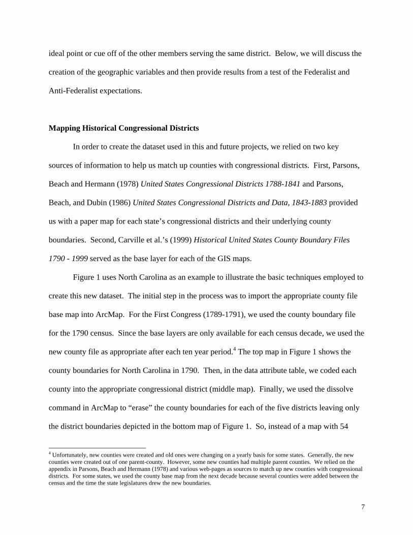
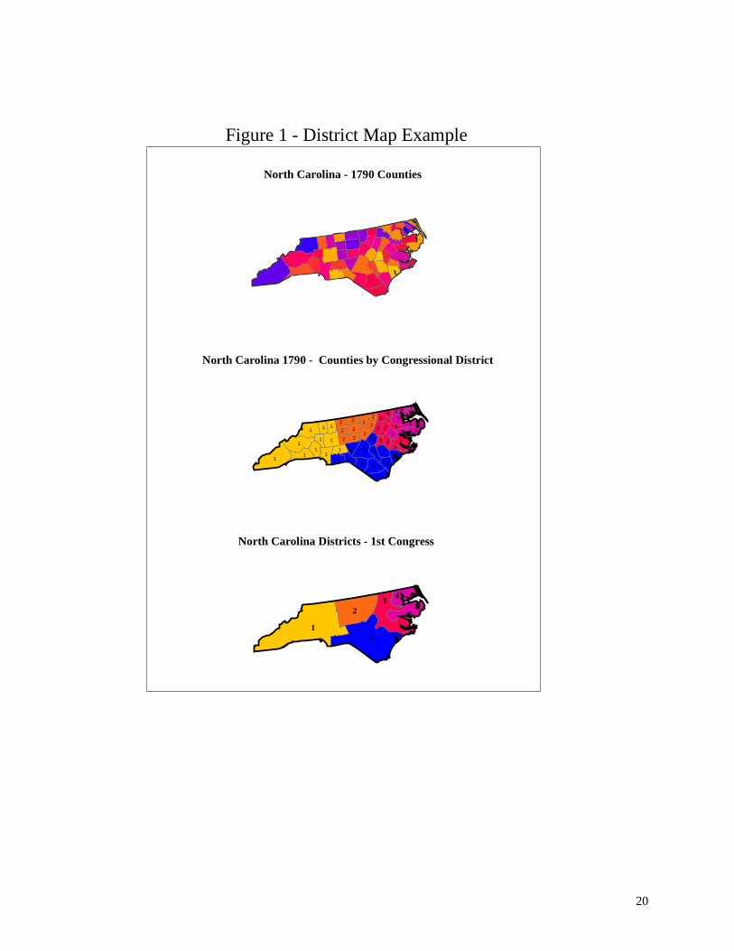
Figure 1 uses North Carolina as an example to illustrate the basic techniques employed to
create this new dataset. The initial step in the process was to import the appropriate county file
base map into ArcMap. For the First Congress (1789-1791), we used the county boundary file
for the 1790 census. Since the base layers are only available for each census decade, we used the
new county file as appropriate after each ten year period.4 The top map in Figure 1 shows the
county boundaries for North Carolina in 1790. Then, in the data attribute table, we coded each
county into the appropriate congressional district (middle map). Finally, we used the dissolve
command in ArcMap to “erase” the county boundaries for each of the five districts leaving only
the district boundaries depicted in the bottom map of Figure 1. So, instead of a map with 54
4 Unfortunately, new counties were created and old ones were changing on a yearly basis for some states. Generally, the new counties were created out of one parent-county. However, some new counties had multiple parent counties. We relied on the appendix in Parsons, Beach and Hermann (1978) and various web-pages as sources to match up new counties with congressional districts. For some states, we used the county base map from the next decade because several counties were added between the census and the time the state legislatures drew the new boundaries.
8
county polygons, we have a new map with five district polygons. Once we formed the new
boundary files for each state, we merged them all together to create a map for each Congress.
We can also take advantage of other features in the GIS program to make the maps more
useful. Since our base layer uses county FIPS as identifiers, we can merge in census and other
data collected at the county level and aggregate it up to the district level. We have also
calculated the area and perimeter of each district so various measures of compactness can be
created. The program also allows us to measure distance between a point in the district and
anywhere else on the map. Finally, we can also designate certain points of interest such as the
various placements of the U.S. Capital.
Generally, the maps are quite similar during each apportionment decade, but occasionally
states would redistrict between census periods or organized state boundaries would change. For
example, New York redistricted between the 5th (1797-1799) and the 6th (1797-1799) Congresses
during the same apportionment period and then drew new boundaries again for the 8th Congress
(1803-1805) after the census of 1800 when it gained 7 additional representatives.5 A careful look
at Figures 2 and 3 indicate that Kentucky was considered part of Virginia during the 1st
Congress. As we move further along in the analysis most of the Indian Lands in the Southeast
disappear and Maine breaks away from Massachusetts.
States were also experimenting with electoral systems at this time so the maps could also
change as election methods changed.6 As displayed in Figure 2, we can see that during the 1st
Congress, three different systems were in place. Massachusetts (which included current state of
Maine), Rhode Island, New York, Delaware, Virginia (which included West Virginia and
5 For more on historical redistricting, see Engstrom (2006). 6 To determine the type of electoral system the state used, we relied on Parson, Beach and Herman (1978) as well as Dubin (1998). If there was a discrepancy between the two sources, we went with the information from Dubin as it is more up to date.

9
Kentucky), North Carolina, and South Carolina all elected their representatives using the now
traditional single-member districts. Other states such as New Hampshire, Connecticut, New
Jersey and Pennsylvania were electing there members at-large from a statewide vote. The
remaining two states, Maryland and Georgia, used a mixed system and selected representatives
from a statewide vote but the members had to be residents of the specific districts designated by
state law.7
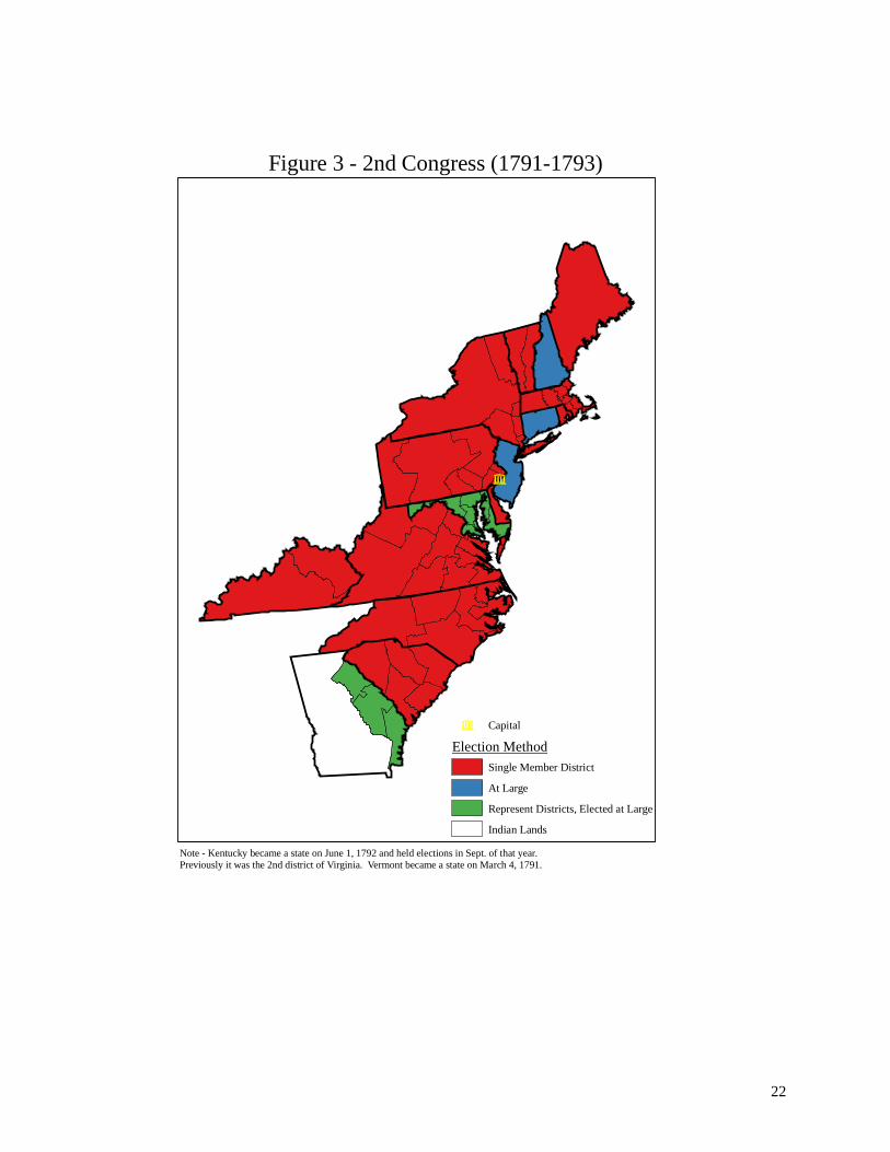
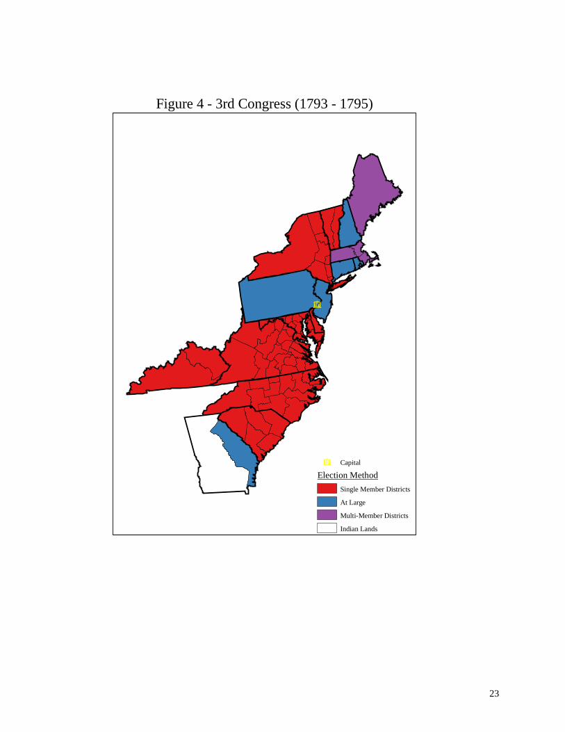
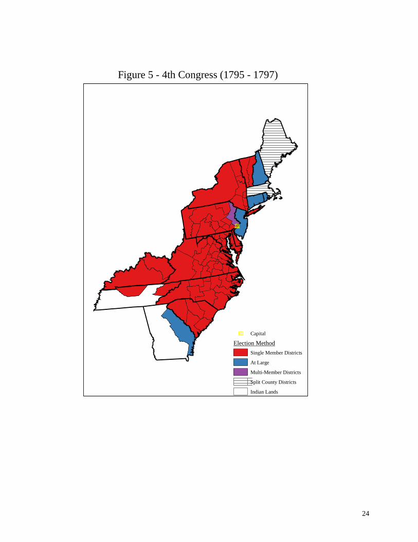
While some states were quite consistent in their methods for electing representatives,
others routinely switched back and forth (see Figures 2 through 5). Pennsylvania, for example,
used an at-large method for the 1st Congress, single member districts for the 2nd (1791-1793), at-
large for the 3rd (1793-1795), and then a mixed system for the 4th (1795-1797). In the mixed
system, 11 of the 12 districts were single member, except for the 4th district which elected two
members. Other states such as Massachusetts and New York occasionally used this type of
electoral system for some districts. Because of the variations in electoral systems, the sporadic
intra-decade redistricting and new states entering the union, we will eventually create a map for
each Congress.
Testing a Spatial Model of Legislator Responsiveness
Data and Measures
To test the influence of geography on representation, we need a variable that can capture
this arguably abstract concept. As our theory suggests, we expect that a member’s voting
behavior in Congress will deviate from their district median depending on factors related to their
district. As such we need to compare measures at both the member and district levels.
7 See Dubin 1998:3 notes 1and 2 for a more detailed description of Georgia and Maryland’s electoral systems.
10
As a proxy for constituency-level preferences, we elected to employ the Democratic
candidate’s share of the two-party presidential vote in each congressional district for Presidential
elections between 1828 and 1844.8 We started with the 1828 election because it was the first
election contested between two parties with a sufficient number of states using a popular vote to
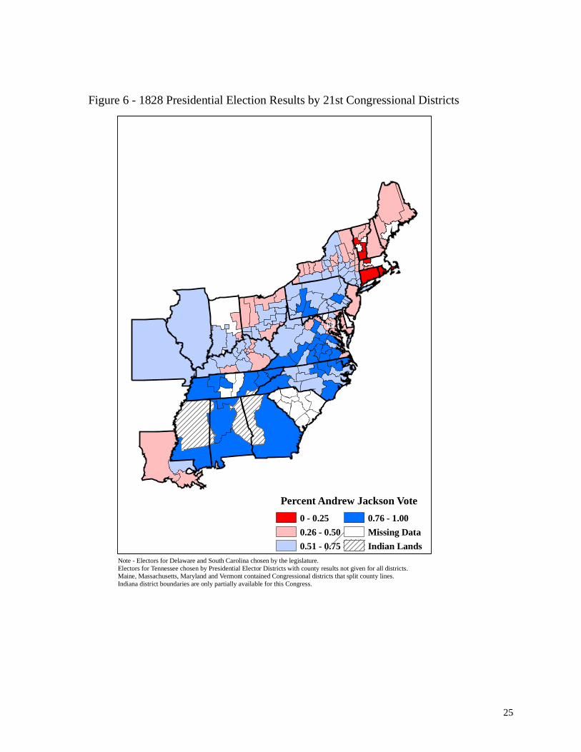
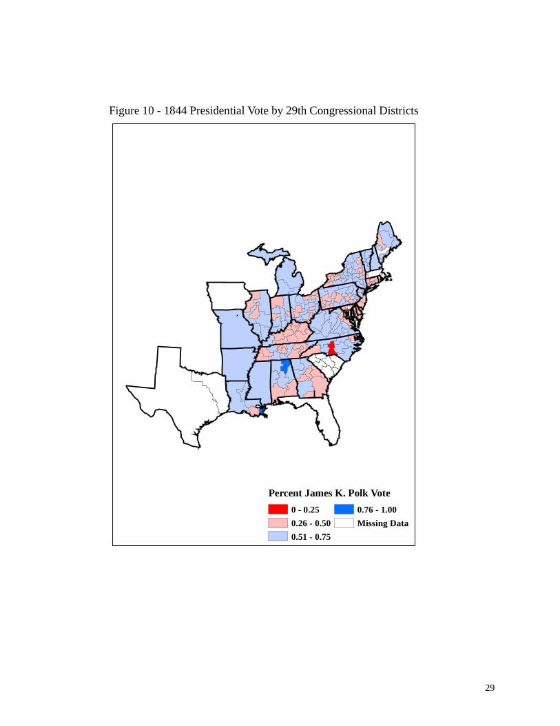
elect presidential electors.9 See Figure 6-10 below for a mapping of the returns at the district
level for the each Presidential election from 1828-1844. These figures, we argue, give us a more
detailed and perhaps meaningful look at presidential election results compared to state level
returns. For example, Figure 6 shows us clear victories for Adams in New England and Jackson
in the Deep South (excluding Louisiana) but mixed results in states like Ohio, New York and
Kentucky. Figures 7 and 8 demonstrate that the Whigs were able to make inroads in some areas
between the 1832 and 1836 elections.
Since this is historical data, election returns do not exist for each and every county. For
example, for the 1828 election, Dubin (2002) lists returns for just over 82% of the counties in
place by the election. In two states that year, Delaware and South Carolina, the electors were
chosen by the state legislature so they were not included in the analysis. For the remaining 22
states, we had at least some county level returns that we could aggregate up to the district level.10
In our analysis below, we excluded most districts in Maine and Massachusetts as well as a
handful of districts where the district boundaries crossed county borders and we could not
disaggregate the county level returns to the sub-county level.11 We have acquired more detailed
maps of most of these districts so in the future, we will include these districts by using lower 8 The advantage of employing district presidential vote is that it provides a more direct measure of the partisan or general ideological predisposition of each congressional district separate from the popularity of the incumbent representing the district (Ansolabehere, Snyder, and Stewart 2000, 2001; Jacobson 2000). 9 We hope to eventually include the 1848, 52 and 56 elections. After this point the two-party system breaks down. 10 Although some states used special districts to select electors, returns were still given at the county level. 11 Initially Maine and Massachusetts elected members from districts based on counties, however, starting with the 4th Congress, most districts no longer followed county boundaries. A preliminary investigation indicates that there was a split within the majority party between rural and urban interests and this lead to the unique districting scheme.

11
level geographic units such as parish or ward data to correctly split the larger county files. We
were also forced to eliminate Indiana from our study in 1828 because the map of the
congressional districts in Parsons, Beach and Hermann (1978:223) appears to be a duplicate of
the map for the 1830 apportionment decade so we are unable to put many of the northern
counties into the correct districts.12 Although there were some problems, we feel we have
enough data to move forward with our analysis.
Next, we measure member’s voting behavior using the standard first dimension DW-
NOMINATE score (Poole and Rosenthal 1997, 2007) for the Congress immediately following
each Presidential election. DW-NOMINATE scores theoretically range from -1 to 1 with
negative scores corresponding to more liberal voting behavior. In order to examine if a
relationship exists between presidential vote in the district (our measure of district preference)
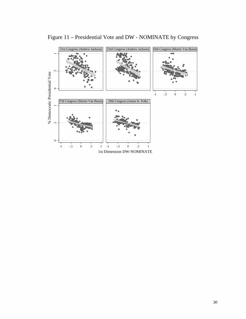
and a member’s voting behavior while in government during this early time period, Figure 11
displays a series of scatterplots between the two measures for each Presidential election congress
pair. We also ran a series of regressions with a member’s nominate score as the dependent
variable and percent Democratic vote share as the independent variable. We found that as the
vote for the Democratic candidate in the district increases, the member’s voting behavior
becomes significantly more liberal. We also plotted each of the regression lines in Figure 10.
Based on a visual examination of the scatterplots and the significant regression results, we feel
we can make a valid claim that presidential vote in the district is providing at least some weight
in terms of a member’s voting behavior in the House.
12 The map given for the 21st Congress depicts seven congressional districts even though Indiana only had three representatives at the time. We are in the process of contacting state archives to get better information so we can include accurate mappings of these states. However, our results are similar if we include these states in our analysis based on the information that we currently possess.
12
Because we need to measure how far a member deviates from his district’s preferences,
and presidential vote and DW-NOMINATE are on two different scales, a simple difference is
probably not the correct was to create our dependent variable for our models. Instead, for each
Congress, we first created z-scores for both measures and then calculated the absolute difference
between the two z-scores. As this new variable gets bigger, a member is further away from his
district median.13 This measure serves as the dependent variable in both of our regressions.
In the regression results below, we have several independent variables that capture
concepts in the debates surrounding the size of the republic and representation. The first three
variables, population, district area, and population density are proxies for district size. Prior to
the “one person, one vote ruling” in Wesberry v. Sanders, there was quite a lot of variation in the
number of constituents in congressional districts within and across states (Engstrom 2005). For
example during the 21st Congress, New York’s 15th district has 35,870 constituents while the
neighboring 14th had 71,326 residents. Both of these are “up-state” districts so these differences
are not necessarily a function of an urban-rural divide. We can also measure district size simply
in terms of geographic area. Here, we measure area in square miles. If the Federalists were
correct, then members who represent more populous and/or larger districts should deviate less
from district preferences and the sign on the coefficient will be negative. If the Anti-Federalists
were correct, then the opposite should hold. To create the next variable, population density, we
calculated the ratio of the total population to the size of the district measured in square miles.
We expect that members who represent a densely populated district should be closer to the
district median so as density increases, our dependent variable should decrease.
13 We must, of course, be careful in presenting marginal effects since our dependent variable lacks meaningful units of measurement.

13
The third and final variable in our first regression is a measure of the total logged
distance between a member’s district and the capital. In the model below, we take the natural
log of the number of miles between the geographic centroid of each district and Washington
D.C. 14 The Anti-Federalists argue that as a member gets further away from district, his ability to
represent the district decreases. Therefore, as distance between the district and the capital
increases, so should the differences between a member’s voting behavior and our measure of
district preferences.15
Findings
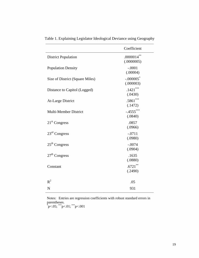
The results of the regression model outlined are in Table 1. The distance from the district
to the capital is positively and significantly related to increased levels of ideological deviance
between the member and their constituents suggesting that the Anti-Federalist argument has
merit. In an age where both communication and transportation were relatively slow, it may well
be that constituents further removed from Washington, geographically speaking, may have had a
more difficult time tracking representative behavior at the capitol. This information asymmetry
created by distance may have allowed representatives a greater amount of voting leeway.
<Table 1 about here>
In addition to violating the one person, one vote standard, malapportioned districts might
also produce differential effects related to representation. As the federal courts have refused to
allow any deviance in regard to population counts for congressional districts within states since
the early 1960’s, examining the linkage between constituent preferences and legislator behavior
can only be studied in the historical realm. Legislators representing districts that contained
14 This is “as the crow flies distance.” Ideally we would have a measure that takes into account both land and water routes but those data are unavailable at this time. We also forced the centriod to reside inside the district. 15 The Federalists do not seem to make an explicit counter argument about distance from the capital.
14
comparatively higher population counts were less likely to deviate from their constituents’
preferences. This analysis indicates that the presence of malapportioned districts might produce
substantive differences in terms of congressional representation but not necessarily in a negative
manner. Likewise, the size of the district represented in terms of square miles is also negatively
and significantly related to legislator deviance. Both of these findings are consistent with the
Federalist notion that more sizable districts, both in terms of geography and population, should
produce better representational outcomes. Surprising, population density, thought to be a proxy
for urbanization, is not a statistically significant predictor of the degree to which a legislator may
diverge from the preferences of constituents.
Finally, we also include dummy variables to identify those states using an at-large
election system to select their House members as well as those members within a state
representing a multi-member district. Compared to members representing a single-member
district, legislators elected at-large display a higher degree of ideological divergence from their
constituents. Conversely, being elected from a multi-member district actually results in a lower
deviance score compared with members representing single-member districts. Apparently, the
behavior of these members may be somewhat constrained by virtue of the fact that other
legislators are dependent upon the exact same electoral base and any large deviance in district
preferences can easily be reported by a member’s district colleague or colleagues. We should
also note the model explains only 5% of the variance in the ideological deviance measure, an
indication that other factors, outside geography, certainly play a role in legislator responsiveness.
The results presented in Table 1 indicate that spatial indicators have a direct effect on the
relationship between legislators’ voting patterns in Congress and preferences of their
constituents. In order to more fully flesh out the tentative relationship found to exist based on
15
these elections, a more stringent set of control variables should be utilized along with the
addition of more temporal observations (presidential elections). We would expect to find that as
technology improves that can enhance communication between representatives and their
constituents, the effects of geography should dissipate.
Discussion
Recently, political scientists have begun to use Geographic Information Systems (GIS) to
study political phenomenon. Through these studies we have learned about interstate conflict
(Berry and Baybeck 2005), electoral competition (Crespin 2005) and turnout (Darmofal 2006).
However, these studies have either been tied to a particular time-period (i.e. the modern era) or a
specific geographic context (i.e. the county). In regard to congressional studies in particular,
much of the empirical literature in this area focuses on the post World War II-era as data are not
readily available from earlier historical time-periods for analysis.
The data created in this project allowed us to directly test parts of the key competing
theories between the first two political parties in the newly created country. Our results suggest
that the Anti-Federalist fear that districts far from the capital will receive “poor” representation
has some empirical backing. On the contrary, their arguments against representative democracy
in large districts do not stand up to empirical tests. In fact, the results back the Federalists notion
that representation is better in larger districts.
The overall goal of this project is to create a dataset suitable for spatial analyses of
congressional districts. In addition to literally mapping districts in an electronic format, we also
plan to match additional political and demographic data to these districts, making historical
empirical analyses a possibility. Only by taking these steps will congressional researchers be

16
able to evaluate theories developed at the time of the founding or compare theories developed in
the post-World War II time period with previous historical periods. In addition, some questions,
such as the one briefly analyzed in this manuscript relating to malapportionment and
representation can only be analyzed in an historical setup.

17
References Altman, Micah. 1998. “Traditional Districting Principles: Judicial Myths vs. Reality.” Social
Science History 22: 159-200.
Ansolabehere, Stephen, James M. Snyder, Jr., and Charles Stewart, III. 2000. “Old Voters, New Voters, and the Personal Vote: Using Redistricting to Measure the Incumbency Advantage.” American Journal of Political Science 44 (January): 17-34.
Ansolabehere, Stephen, James M. Snyder, Jr., and Charles Stewart, III. 2001. “Candidate Positioning in U.S. House Elections.” American Journal of Political Science 45 (January): 136-159.
Berry, William, and Brady Baybeck. 2005. “Using Geographic Information Systems to Study Interstate Competition.” American Political Science Review, 99:505-19.
Bianco, William T., David B. Spence, and John D. Wilkerson. 1996. “The Electoral Connection in the Early Congress: The Case of the Compensation Act of 1816.” American Journal of Political Science 40: (February):145–71.
Brunell, Thomas L.. and Bernard Grofman. 1998. “Explaining divided U.S. Senate delegations. 1988-1996: A realignment approach.” American Political Science Review 92:391-411.
Carson, Jamie L. and Erik Engtstrom. 2005. “Assessing the Electoral Connection: Evidence from the Early United States,” American Journal of Political Science 49(4): 746–757
Cho, Wendy K. 2003. “Contagion Effects and Ethnic Contribution Networks.” American Journal of Political Science 47(2): 368-87.
Cox, Gary W. and Jonathan N. Katz. 2002. Elbridge Gerry’s Salamander: The Electoral Consequences of the Reapportionment Revolution. New York: Cambridge University Press.
Crespin, Michael H. 2005. “Using Geographic Information Systems to Measure District Change, 2000-02,” Political Analysis 13(3): 253-260.
Darmofal, David. 2006. “The Political Geography of Macro-Level Turnout in American Political Development.” Political Geography 25(2): 123-150.
Dubin, Michael J. 1998. United States Congressional Elections, 1788-1997: The Official Results. Jefferson, North Carolina: McFarland & Company.
Dubin, Michael J. 2002. United States Presidential Elections, 1788-1860: The Official
Results by County and State. Jefferson, North Carolina: McFarland & Company.
18
Earle, Carville, Changyong Cao, John Heppen, and Samuel Otterstrom. 1999. The Historical
United States County Boundary Files 1790 - 1999 on CD-ROM. Geoscience Publications. Louisiana State University.
Engstrom, Erik. 2006. “Stacking the States, Stacking the House: The Partisan Consequences of
Redistricting in the 19th Century.” American Political Science Review 100:419-427. Engstrom, Erik. 2005. “The Partisan Impact of Malapportionment on the 19th Century and Early
20th Century House of Representatives.” Paper presented at the Midwestern Political Science Association Annual Meeting, Chicago. IL.
Erikson, Robert S. 1972. “Malapportionment, Gerrymandering, and Party Fortunes.” The
American Political Science Review 66: 1234-1245.
Fiorina, Morris P. 1992. Divided Government. New York: Macmillan. Gimpel, James G., Frances E. Lee and Joshua Kaminski. 2006. “The Political
Geography of Campaign Contributions in American Politics,” The Journal of Politics 68(3): 626-639.
Jacobson, Gary C. 2000. “Party Polarization in National Politics: The Electoral Connection.” In Polarized Politics: Congress and the President in a Partisan Era. Jon R. Bond and Richard Fleisher, editors. Washington, DC: CQ Press, 9-30.
Niemi, Richard G., Bernard Grofman, Carl Carlucci, and Thomas Hofeller. 1990. “Measuring Compactness and the Role of a Compactness Standard in a Test for Partisan and Racial Gerrymandering,” The Journal of Politics, 52(4): 1155-1181.
Parsons, Stanly B., William W. Beach and Dan Hermann. 1978. United States Congressional Districts 1788-1841, Westport, CT: Greenwood Press:.
Parsons, Stanley B., William W. Beach and, Michael J. Dubin. 1986. United States
Congressional Districts and Data, 1843-1883. New York : Greenwood Press. . Poole, Keith T. and Howard Rosenthal. 1997. Congress: A Political-Economic History of Roll Call Voting. New York: Oxford University Press. Poole, Keith T. and Howard Rosenthal. 2007. Ideology and Congress. New Brunswick, N.J.: Transaction Publishers. Storing, Herbert J. 1981. What the Anti-Federalists were for. Chicago, IL: University of
Chicago. Tufte, Edward R. 1973. “The Relationship between Seats and Votes in Two-Party Systems.”
The American Political Science Review 67:540-554.
19
Table 1. Explaining Legislator Ideological Deviance using Geography
Coefficient
District Population .0000014** (.0000005)
Population Density -.0001
(.00004)
Size of District (Square Miles) -.000005* (.000003)
Distance to Capitol (Logged) .1421*** (.0430)
At-Large District .5861*** (.1472)
Multi-Member District -.4555*** (.0840)
21st Congress .0857 (.0966)
23rd Congress -.0711 (.0980)
25th Congress -.0074 (.0904)
27th Congress .1635 (.0880)
Constant .6721**
(.2490)
R2 .05
N 931
Notes: Entries are regression coefficients with robust standard errors in parentheses. *p<.05; ***p<.01; ***p<.001
20
Figure 1 - District Map Example
15
23 4
1
1
1
5
5
1
1
3
11
5
2 4
5
1 5
55
2
5
11
4
5
555
2
2
3
1
34
2
322
3
22
3
24
3
4
3 4
3
44 444
4
4 4
4
North Carolina - 1790 Counties
North Carolina 1790 - Counties by Congressional District
North Carolina Districts - 1st Congress

21
ñ
ñ Capital
Election MethodSingle Member District
At Large
Represent Districts, Elected at Large
Indian Lands
Figure 2 - 1st Congress (1789 - 1791)
22
ñ
Figure 3 - 2nd Congress (1791-1793)
Note - Kentucky became a state on June 1, 1792 and held elections in Sept. of that year.Previously it was the 2nd district of Virginia. Vermont became a state on March 4, 1791.
ñ Capital
Election MethodSingle Member District
At Large
Represent Districts, Elected at Large
Indian Lands
23
ñ
Figure 4 - 3rd Congress (1793 - 1795)
ñ Capital
Election MethodSingle Member Districts
At Large
Multi-Member Districts
Indian Lands
24
ñ
ñ Capital
Election MethodSingle Member Districts
At Large
Multi-Member Districts
Split County Districts
Indian Lands
Figure 5 - 4th Congress (1795 - 1797)
25
ñ
Figure 6 - 1828 Presidential Election Results by 21st Congressional Districts
Percent Andrew Jackson Vote0 - 0.250.26 - 0.500.51 - 0.75
0.76 - 1.00Missing DataIndian Lands
Note - Electors for Delaware and South Carolina chosen by the legislature. Electors for Tennessee chosen by Presidential Elector Districts with county results not given for all districts. Maine, Massachusetts, Maryland and Vermont contained Congressional districts that split county lines. Indiana district boundaries are only partially available for this Congress.

26
ñ
Percent Andrew Jackson Vote0 - 0.250.26 - 0.500.51 - 0.75
0.76 - 1.00Missing DataIndian Lands
Figure 7 - 1832 Presidential Vote by 23rd Congressional Districts

27
ñ
Percent Martin Van Buren Vote
0 - 0.250.26 - 0.500.51 - 0.75
0.76 - 1.00Missing DataIndian Land
Figure 8 - 1836 Presidential Vote by 25th Congressional Districts

28
ñ
Percent Martin Van Buren Vote
0.23 - 0.250.26 - 0.500.51 - 0.75
0.76 - 1.00Missing DataIndian Lands
Figure 9 - 1840 Presidential Vote by 27th Congressional Districts
29
ñ
Percent James K. Polk Vote0 - 0.250.26 - 0.500.51 - 0.75
0.76 - 1.00Missing Data
Figure 10 - 1844 Presidential Vote by 29th Congressional Districts
30
Figure 11 – Presidential Vote and DW - NOMINATE by Congress
0.5
10
.51
-1 -.5 0 .5 1
-1 -.5 0 .5 1 -1 -.5 0 .5 1
21st Congress (Andrew Jackson) 23rd Congress (Andrew Jackson) 25th Congress (Martin Van Buren)
27th Congress (Martin Van Buren) 29th Congress (James K. Polk)
% D
emoc
ratic
Pre
side
ntia
l Vot
e
1st Dimension DW-NOMINATE