backward modeling of thermal convection: a new numerical approach applied to plume reconstruction...
TRANSCRIPT

Backward modeling of thermal convection: a new numerical approach
applied to plume reconstruction
Evgeniy Tantserev Collaborators: Marcus Beuchert and Yuri Podladchikov

OverviewOverview
Introduction Introduction Thermal convection problemThermal convection problem Forward and Backward Heat Conduction Problem Forward and Backward Heat Conduction Problem Pseudo-parabolic approach to solve BHCPPseudo-parabolic approach to solve BHCP Forward and backward modeling of thermal Forward and backward modeling of thermal
convection problem for high Rayleigh numberconvection problem for high Rayleigh number Forward and backward modeling of thermal Forward and backward modeling of thermal
convection problem for low Rayleigh number: convection problem for low Rayleigh number: different techniquesdifferent techniques
ConclusionsConclusions

Geological Geological pastpast is reconstructed using is reconstructed using presentpresent day day observations. It is an observations. It is an inverseinverse problem known to be problem known to be ill- ill- posedposed..
Numerous new modeling directions became feasible due to Numerous new modeling directions became feasible due to the growth of computer power. Most of these new modeling the growth of computer power. Most of these new modeling attempts are “attempts are “forwardforward” in time because they deal with ” in time because they deal with irreversibleirreversible processes. processes.
However, However, geological structuresgeological structures often formed by often formed by instabilitiesinstabilities. . Instabilities are often Instabilities are often easiereasier to simulate to simulate inverse (reverse) in inverse (reverse) in timetime..
Practical Practical numericalnumerical recipes and recipes and mathematicalmathematical understanding of understanding of time “inversion”time “inversion” of instabilitiesof instabilities is in great is in great and urgent need in the geodynamics.and urgent need in the geodynamics.
”Approach your problem from the right end and begin with answers. Then one day, perhaps you will find the final question.”
From ”The Hermit Clad in Crane Feathers” in the Chinese Maze Murders, by R. Van Gulik
IntroductionIntroduction

Well-posed problem
Existence Uniqueness Stability
Ill-posed problem
Non-existence Non-uniqueness Non-stability
For the well-posedness should be all three conditions
For the ill-posedness enough the existence of one condition
IntroductionIntroduction

IntroductionIntroduction
Mantle plumes are among the most spectacular features of mass and heat transport from the mantle to the Earth’s surface. Forward modeling requires starting from generic initial temperature distributions in the mantle and follows the evolution of arising mantle plumes
Temperature

Thermal convection problemThermal convection problem
3
0
,ig ThRa
λ is a non-dimensional activation parameter
The thermal convection of mantle plumes is mainly driven by two processes:
advection and thermal diffusion.
Initial profile of the temperature: steady- state distribution with initial perturbation with added noise of maximum amplitude 1 %.
* * *( ) TT e
* * 0,iiv
* * * * * * * * * * ,ij i jj j j i iP T v v RaT
**2 * * *
*,i
i i
TT v T
t
As boundary conditions on the top we put temperature T=-0.5 and on the bottom T=0.5. And we have periodic boundary conditions on the sides.

2
f2
f
f
( , ) for x in (0,1) - 1d size of our object, t in (0,t ) our time.
(0, ) 0 for t in (0,t ),
(1, ) 0 for t in (0,t ),
( ,0) sin( ) for x in (0,1).
T Tx t
t xT t
T t
T x x
2
T(x,0) sin( x)
T(x,t) sin( x)exp(- ).t
boundary conditions
initial distribution of temperature
The forward problem is to find the final final distribution of temperaturedistribution of temperature (for time tf ) for given heat conduction law, boundary conditions and initial distribution of temperature .
Forward Heat conduction – well-posed problemForward Heat conduction – well-posed problem

(0,1).in for x )(),(
),t(0,in for t 0),1(
),t(0,in for t 0),0(
our time. )t(0,in t object,our of size 1d - (0,1)in for x ),(
f
f
f2
2
xgtxT
tT
tTx
Ttx
t
T
f
boundary conditions
The Final distribution of temperature
The inverse problem is to find the initial distribution of temperature (for time t0) for given heat conduction law, boundary conditions and final distribution of
temperature
Initial distribution of temperature, which we need to obtain!
Final distribution of temperature which we know from experimental data
Backward Heat conduction – ill-posed problem

Initial distribution of temperature, which we need to obtain
Final distribution of temperature which we know from experimental data
The pseudo-parabolic reversibilityThe pseudo-parabolic reversibilitymethodmethod
Regularized BHCP – well-posed problem
2
2( , , ) = 0
T
t
x
Tx y t T
t

1.Heat diffusion and viscous flow problem – FEM using Galerkin method
2.Advection problem - method of backward characteristics
Forward modeling of plumes

Reverse modeling for this case was done, using the same code as for forward but with negative time steps.
This problem is relatively stable because for high Ra number we have domination of advection process over the diffusion process
Reverse modeling of thermal convection problem for high Rayleigh number

Forward problem
TRM is highly unstable for this case due to increasing influence of diffusion term
1.Time Reverse Method change sign of the time-step from positive to negative one and use the same code
Forward and Backward modeling of thermal convection for low Rayleigh number

2. Using Tichonov RegularizationWe use TRM but every 3rd time step we change sign of time step from negative to positive one and solving forward heat diffusion problem we regularize the solution of thermo-convective problem
Forward and Backward modeling of thermal convection for low Rayleigh number

PPB approach let us to evaluate temperature distribution for a longer backward time
3. Pseudo-parabolic approach (PPB) with regularized parameter ε = 10^-2
Forward and Backward modeling of thermal convection for low Rayleigh number

1.Time Reverse method
2. Using Tichonov’s Regularization
3. Pseudo-parabolic approach with regularized parameter e = 10^-2
Forw
ard
and B
ackw
ard
modelin
g fo
r low
Rayle
igh n
um
ber
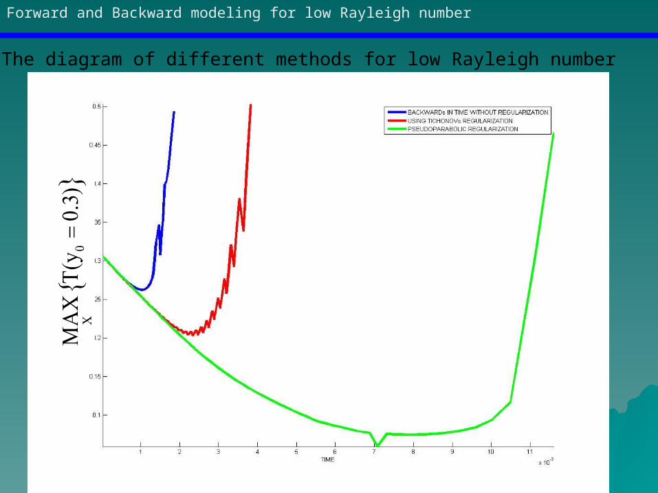
The diagram of different methods for low Rayleigh number
Forward and Backward modeling for low Rayleigh number

ConclusionsConclusions For high Ra number (in our case 9*10^6) backward For high Ra number (in our case 9*10^6) backward
modeling of mantle plumes is relatively stable.modeling of mantle plumes is relatively stable. For low Ra number(2*10^5) we need to apply additional For low Ra number(2*10^5) we need to apply additional
techniques to model backward process techniques to model backward process Time reverse method for this case of Rayleigh number is Time reverse method for this case of Rayleigh number is
highly unstable, method based on Tichonov’s regularization highly unstable, method based on Tichonov’s regularization is more stable and pseudo-parabolic method is the most is more stable and pseudo-parabolic method is the most stable in time reverse restoration of the temperature profilestable in time reverse restoration of the temperature profile
PPB approach is perspective method for restoration of PPB approach is perspective method for restoration of temperature profile of mantle plumes temperature profile of mantle plumes

Thank you for your attention!
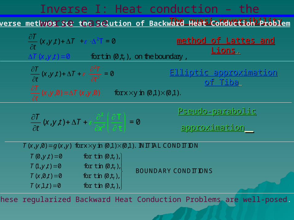
The quasi-reversibility The quasi-reversibility method of Lattes and Lionsmethod of Lattes and Lions..2
f
( , , ) + = 0
for t in (0,t ), on the
T
( , , bounda ) ry ,0 T x y
Tx y
t
t Tt
2
2( , , ) = 0
T
t
x
Tx y t T
t
2
2
( , ,0
( , , ) = 0
for x y in () ( , 0,1) (,0) 0,1).
T
tTx y T
Tx y t T
y
t
xt
Elliptic approximation of TibaElliptic approximation of Tiba
Pseudo-parabolic approximationPseudo-parabolic approximation
f
f
f
f
(0, , ) 0 for t in (0,t ),
(1, , ) 0 for t in (0,t ),BOUNDARY CONDITIONS
( ,0, ) 0 for t in (0,t ),
( ,1, ) 0 for t in (0,t ),
T y t
T y t
T x t
T x t
( , ,0) ( , ) for x y in (0,1) (0,1). INITIAL CONDITIONT x y g x y
Reverse methods for the solution of Backward Heat Conduction Problem
These regularized Backward Heat Conduction Problems are well-posed.
Inverse I: Heat conduction – the worse case

Applications of the reversibility’s methods to the solution of Backward Heat Conduction Problem
| ||| || max 0.25
| |an
an
T TT T
T
analytical solutions for three regularized BHCP,
analytical solution for original BHCP
ianT
T
The diagrams show which method works better for analytical solutions for different frequencies and regularized parameters, that is differences between analytical solution regularized problem and original
problem in the norm smaller fixed constant for longest time.
Inverse I: Heat conduction – the worse case