bài 3-tt dsp
DESCRIPTION
Bài 3-TT DSPTRANSCRIPT

Name : Vo Phong Phu - 10117050
Laboratory Exercise 3
DISCRETE-TIME SIGNALS: FREQUENCY-DOMAIN REPRESENTATIONS
3.1 DISCRETE-TIME FOURIER TRANSFORM
Project 3.1 DTFT Computation
A copy of Program P3_1 is given below:
% Program P3_1
% Evaluation of the DTFT
clf;
% Compute the frequency samples of the DTFT
w = -4*pi:8*pi/511:4*pi;
num = [2 1];den = [1 -0.6];
h = freqz(num, den, w);
% Plot the DTFT
subplot(2,1,1)
plot(w/pi,real(h));grid
title('Real part of H(e^{j\omega})')
xlabel('\omega /\pi');
ylabel('Amplitude');
subplot(2,1,2)
plot(w/pi,imag(h));grid
title('Imaginary part of H(e^{j\omega})')
xlabel('\omega /\pi');
ylabel('Amplitude');
pause
subplot(2,1,1)
plot(w/pi,abs(h));grid
title('Magnitude Spectrum |H(e^{j\omega})|')
xlabel('\omega /\pi');
ylabel('Amplitude');
subplot(2,1,2)
plot(w/pi,angle(h));grid
title('Phase Spectrum arg[H(e^{j\omega})]')
xlabel('\omega /\pi');
ylabel('Phase in radians');
Answers:
Q3.1 The expression of the DTFT being evaluated in Program P3_1 is
H(jw)=
2+e− jw
1−0 . 6e− jw
The function of the pause command is used to wait for user response by press any keys.
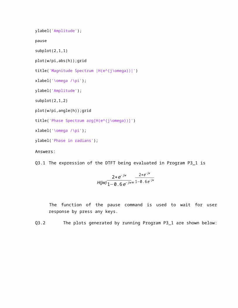
Q3.2 The plots generated by running Program P3_1 are shown below:
-4 -3 -2 -1 0 1 2 3 40
2
4
6
8Real part of H(ej)
/
Am
plitu
de
-4 -3 -2 -1 0 1 2 3 4-4
-2
0
2
4Imaginary part of H(ej)
/
Am
plitu
de

-4 -3 -2 -1 0 1 2 3 40
2
4
6
8Magnitude Spectrum |H(ej)|
/
Am
plitu
de
-4 -3 -2 -1 0 1 2 3 4-2
-1
0
1
2Phase Spectrum arg[H(ej)]
/
Phase in r
adia
ns
The DTFT is a continuous function of .
Its period is 2π.
The types of symmetries exhibited by the four plots are as follows:
• The real part is 2 π periodic and EVEN SYMMETRIC.
• The imaginary part is 2π periodic and ODD SYMMETRIC.
• The magnitude is 2 π periodic and EVEN SYMMETRIC.
• The phase is 2 π periodic and ODD SYMMETRIC.
Q3.3 The required modifications to Program P3_1 to evaluate the given DTFT of Q3.3 are given below:
clf;
clc;
% Compute the frequency samples of the DTFT
w = 0:pi/511:pi;
num = [0.7 -0.5 0.3 1];
den = [1 0.3 -0.5 0.7];
h = freqz(num, den, w);
% Plot the DTFT
subplot(2,1,1)

plot(w/pi,real(h));grid
title('Real part of H(e^{j\omega})')
xlabel('\omega /\pi');
ylabel('Amplitude');
subplot(2,1,2)
plot(w/pi,imag(h));grid
title('Imaginary part of H(e^{j\omega})')
xlabel('\omega /\pi');
ylabel('Amplitude');
pause
subplot(2,1,1)
plot(w/pi,abs(h));grid
title('Magnitude Spectrum |H(e^{j\omega})|')
xlabel('\omega /\pi');
ylabel('Amplitude');
subplot(2,1,2)
plot(w/pi,angle(h));grid
title('Phase Spectrum arg[H(e^{j\omega})]')
xlabel('\omega /\pi');
ylabel('Phase in radians');
The plots generated by running the modified Program P3_1 are shown below:
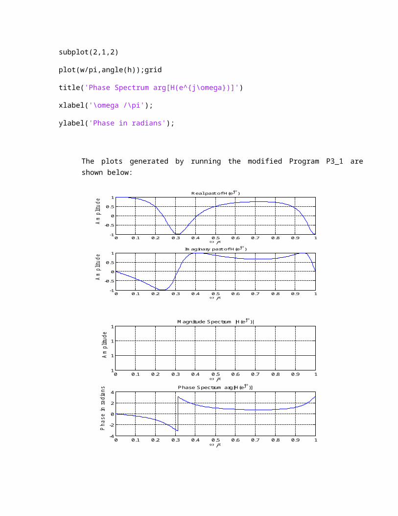
0 0.1 0.2 0.3 0.4 0.5 0.6 0.7 0.8 0.9 1-1
-0.5
0
0.5
1Real part of H(ej)
/A
mplitu
de
0 0.1 0.2 0.3 0.4 0.5 0.6 0.7 0.8 0.9 1-1
-0.5
0
0.5
1Imaginary part of H(ej)
/
Am
plitu
de
0 0.1 0.2 0.3 0.4 0.5 0.6 0.7 0.8 0.9 11
1
1
1Magnitude Spectrum |H(ej)|
/
Am
plitu
de
0 0.1 0.2 0.3 0.4 0.5 0.6 0.7 0.8 0.9 1-4
-2
0
2
4Phase Spectrum arg[H(ej)]
/
Phase in r
adia
ns
The DTFT is a continuous function of .
Its period is 2π.
The jump in the phase spectrum is caused by the angle command. It give the angle lie between ±π.
The phase spectrum evaluated with the jump removed by the command unwrap is as given below:
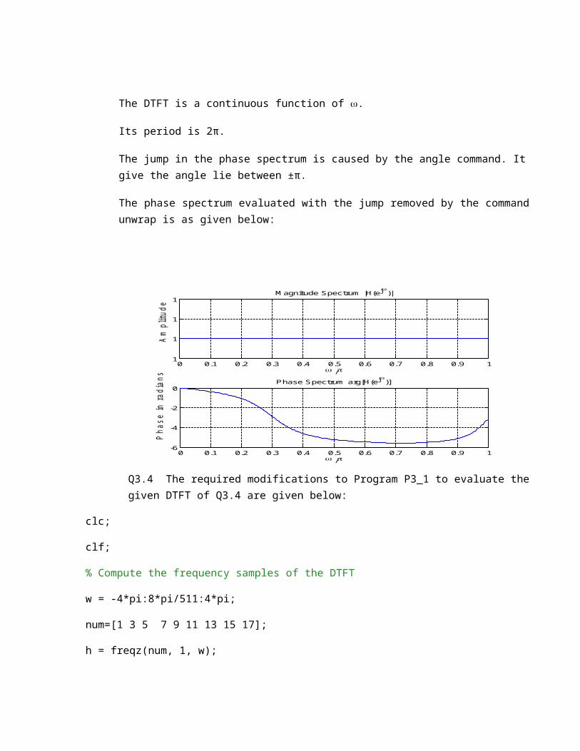
0 0.1 0.2 0.3 0.4 0.5 0.6 0.7 0.8 0.9 11
1
1
1Magnitude Spectrum |H(ej)|
/
Am
plitu
de
0 0.1 0.2 0.3 0.4 0.5 0.6 0.7 0.8 0.9 1-6
-4
-2
0Phase Spectrum arg[H(ej)]
/
Phase in r
adia
ns
Q3.4 The required modifications to Program P3_1 to evaluate the given DTFT of Q3.4 are given below:
clc;
clf;
% Compute the frequency samples of the DTFT
w = -4*pi:8*pi/511:4*pi;
num=[1 3 5 7 9 11 13 15 17];
h = freqz(num, 1, w);
% Plot the DTFT
subplot(2,1,1)
plot(w/pi,real(h));grid
title('Real part of H(e^{j\omega})')
xlabel('\omega /\pi');
ylabel('Amplitude');
subplot(2,1,2)
plot(w/pi,imag(h));grid
title('Imaginary part of H(e^{j\omega})')
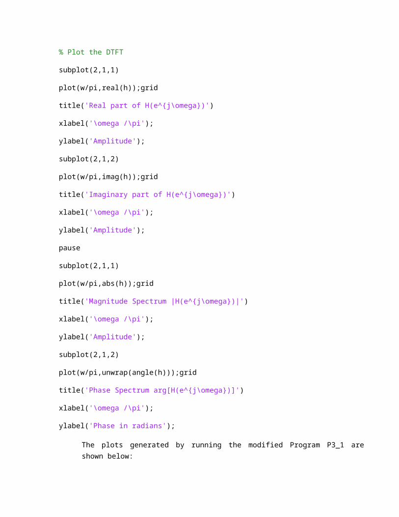
xlabel('\omega /\pi');
ylabel('Amplitude');
pause
subplot(2,1,1)
plot(w/pi,abs(h));grid
title('Magnitude Spectrum |H(e^{j\omega})|')
xlabel('\omega /\pi');
ylabel('Amplitude');
subplot(2,1,2)
plot(w/pi,unwrap(angle(h)));grid
title('Phase Spectrum arg[H(e^{j\omega})]')
xlabel('\omega /\pi');
ylabel('Phase in radians');
The plots generated by running the modified Program P3_1 are shown below:
-4 -3 -2 -1 0 1 2 3 4-50
0
50
100Real part of H(ej)
/
Am
plitu
de
-4 -3 -2 -1 0 1 2 3 4-100
-50
0
50
100Imaginary part of H(ej)
/
Am
plitu
de

-4 -3 -2 -1 0 1 2 3 40
50
100Magnitude Spectrum |H(ej)|
/
Am
plitude
-4 -3 -2 -1 0 1 2 3 4-4
-2
0
2
4Phase Spectrum arg[H(ej)]
/
Phase in radia
ns
The DTFT is a continuous function of .
Its period is 2π.
The jump in the phase spectrum is caused by the same reason in Q3.3.
Q3.5 The required modifications to Program P3_1 to plot the phase in degrees are indicated below:
subplot(2,1,2)
plot(w/pi*180,angle(h)*180/pi);grid
title('Phase Spectrum arg[H(e^{j\omega})]')
xlabel('Degrees');
ylabel('Phase in degrees');
We get observation :
-4 -3 -2 -1 0 1 2 3 40
2
4
6
8Magnitude Spectrum |H(ej)|
/
Am
plitu
de
-800 -600 -400 -200 0 200 400 600 800-100
-50
0
50
100Phase Spectrum arg[H(ej)]
Degrees
Phase in d
egre
es
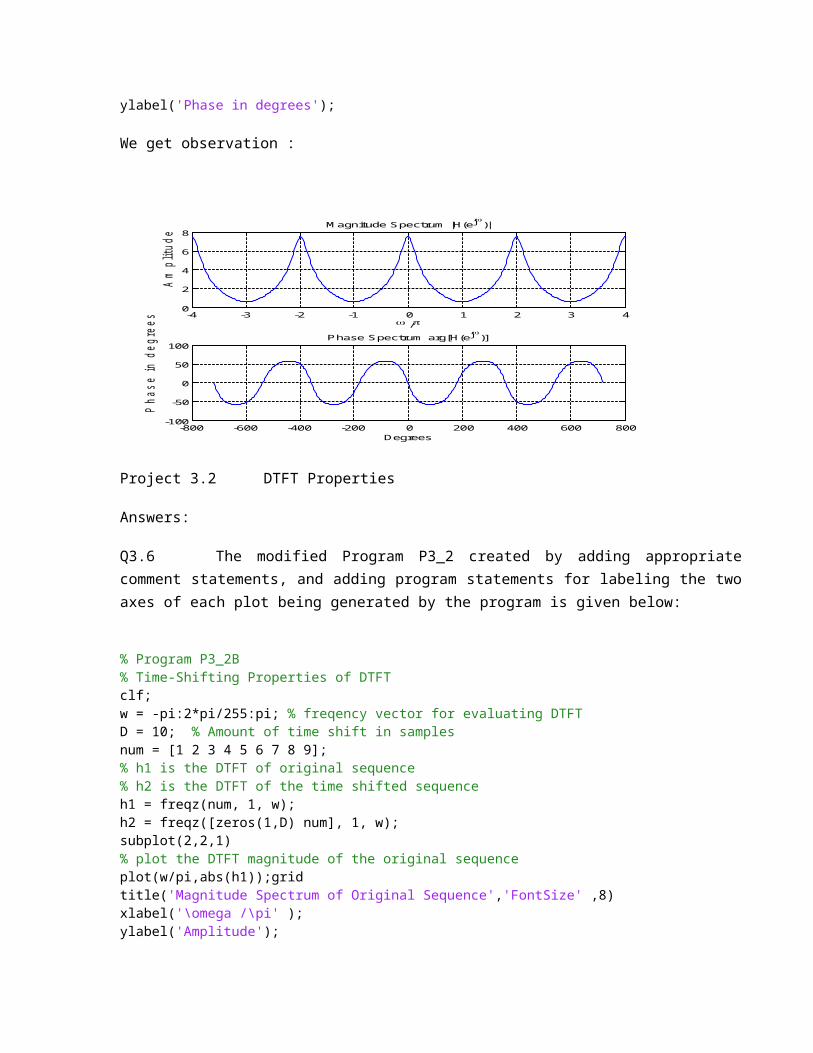
Project 3.2 DTFT Properties
Answers:
Q3.6 The modified Program P3_2 created by adding appropriate comment statements, and adding program statements for labeling the two axes of each plot being generated by the program is given below:
% Program P3_2B % Time-Shifting Properties of DTFT clf; w = -pi:2*pi/255:pi; % freqency vector for evaluating DTFT D = 10; % Amount of time shift in samples num = [1 2 3 4 5 6 7 8 9]; % h1 is the DTFT of original sequence % h2 is the DTFT of the time shifted sequence h1 = freqz(num, 1, w); h2 = freqz([zeros(1,D) num], 1, w); subplot(2,2,1) % plot the DTFT magnitude of the original sequence plot(w/pi,abs(h1));grid title('Magnitude Spectrum of Original Sequence','FontSize' ,8) xlabel('\omega /\pi' ); ylabel('Amplitude'); % plot the DTFT magnitude of the shifted sequence subplot(2,2,2) plot(w/pi,abs(h2));grid title('Magnitude Spectrum of Time-Shifted Sequence' ,'FontSize' ,8) xlabel('\omega /\pi' ); ylabel('Amplitude'); % plot the DTFT phase of the original sequence subplot(2,2,3) plot(w/pi,angle(h1));grid title('Phase Spectrum of Original Sequence','FontSize' ,8) xlabel('\omega /\pi' ); ylabel('Phase in radians' ); % plot the DTFT phase of the shifted sequence subplot(2,2,4) plot(w/pi,angle(h2));grid title('Phase Spectrum of Time-Shifted Sequence','FontSize' ,8) xlabel('\omega /\pi' ); ylabel('Phase in radians' );
The parameter controlling the amount of time-shift is D
Q3.7 The plots generated by running the modified program are given below:

-1 -0.5 0 0.5 10
20
40
60Magnitude Spectrum of Original Sequence
-1 -0.5 0 0.5 10
20
40
60Magnitude Spectrum of Time-Shifted Sequence
-1 -0.5 0 0.5 1-4
-2
0
2
4Phase Spectrum of Original Sequence
-1 -0.5 0 0.5 1-4
-2
0
2
4Phase Spectrum of Time-Shifted Sequence
From these plots we make the following observations:
The magnitude spectrum is not changed.
Shift in time-domain is shrink in frequency-domain. The phase changes rapidly.
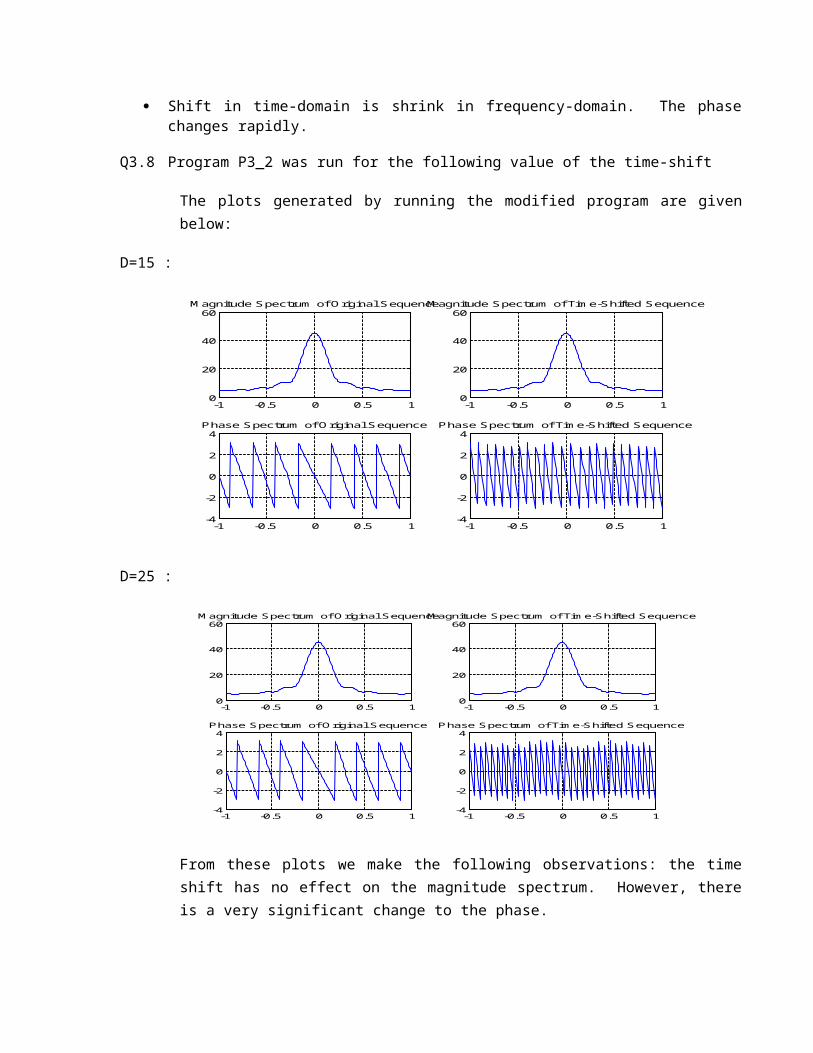
Q3.8 Program P3_2 was run for the following value of the time-shift
The plots generated by running the modified program are given below:
D=15 :
-1 -0.5 0 0.5 10
20
40
60Magnitude Spectrum of Original Sequence
-1 -0.5 0 0.5 10
20
40
60Magnitude Spectrum of Time-Shifted Sequence
-1 -0.5 0 0.5 1-4
-2
0
2
4Phase Spectrum of Original Sequence
-1 -0.5 0 0.5 1-4
-2
0
2
4Phase Spectrum of Time-Shifted Sequence
D=25 :
-1 -0.5 0 0.5 10
20
40
60Magnitude Spectrum of Original Sequence
-1 -0.5 0 0.5 10
20
40
60Magnitude Spectrum of Time-Shifted Sequence
-1 -0.5 0 0.5 1-4
-2
0
2
4Phase Spectrum of Original Sequence
-1 -0.5 0 0.5 1-4
-2
0
2
4Phase Spectrum of Time-Shifted Sequence
From these plots we make the following observations: the time shift has no effect on the magnitude spectrum. However, there is a very significant change to the phase.
The higher delay-time is, the higher shrink is. The phase changes more rapidly.
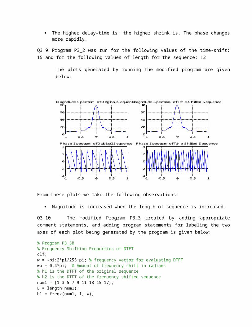
Q3.9 Program P3_2 was run for the following values of the time-shift: 15 and for the following values of length for the sequence: 12
The plots generated by running the modified program are given below:
-1 -0.5 0 0.5 10
20
40
60
80Magnitude Spectrum of Original Sequence
-1 -0.5 0 0.5 10
20
40
60
80Magnitude Spectrum of Time-Shifted Sequence
-1 -0.5 0 0.5 1-4
-2
0
2
4Phase Spectrum of Original Sequence
-1 -0.5 0 0.5 1-4
-2
0
2
4Phase Spectrum of Time-Shifted Sequence
From these plots we make the following observations:
Magnitude is increased when the length of sequence is increased.
Q3.10 The modified Program P3_3 created by adding appropriate comment statements, and adding program statements for labeling the two axes of each plot being generated by the program is given below:
% Program P3_3B % Frequency-Shifting Properties of DTFT clf; w = -pi:2*pi/255:pi; % frequency vector for evaluating DTFT wo = 0.4*pi; % Amount of frequency shift in radians % h1 is the DTFT of the original sequence % h2 is the DTFT of the frequency shifted sequence num1 = [1 3 5 7 9 11 13 15 17]; L = length(num1); h1 = freqz(num1, 1, w); n = 0:L-1; num2 = exp(wo*i*n).*num1; h2 = freqz(num2, 1, w); % plot the DTFT magnitude of the original sequence subplot(2,2,1) plot(w/pi,abs(h1));grid title('Magnitude Spectrum of Original Sequence','FontSize' ,8) xlabel('\omega /\pi' ); ylabel('Amplitude'); % plot the DTFT magnitude of the freq shifted sequence subplot(2,2,2) plot(w/pi,abs(h2));grid title('Magnitude Spectrum of Frequency-Shifted Sequence' ,'FontSize' ,8) xlabel('\omega /\pi' ); ylabel('Amplitude'); % plot the DTFT phase of the original sequence subplot(2,2,3) plot(w/pi,angle(h1));grid title('Phase Spectrum of Original Sequence','FontSize' ,8) xlabel('\omega /\pi' ); ylabel('Phase in radians' ); % plot the DTFT phase of the shifted sequence subplot(2,2,4) plot(w/pi,angle(h2));grid title('Phase Spectrum of Frequency-Shifted Sequence','FontSize' ,8) xlabel('\omega /\pi' ); ylabel('Phase in radians' );
The parameter controlling the amount of frequency-shift is “wo”.
Q3.11 The plots generated by running the modified program are given below:
-1 -0.5 0 0.5 10
50
100Magnitude Spectrum of Original Sequence
-1 -0.5 0 0.5 10
50
100Magnitude Spectrum of Frequency-Shifted Sequence
-1 -0.5 0 0.5 1-4
-2
0
2
4Phase Spectrum of Original Sequence
-1 -0.5 0 0.5 1-4
-2
0
2
4Phase Spectrum of Frequency-Shifted Sequence
From these plots we make the following observations:
Magnitude spectrum of frequency shifted sequence and phase spectrum are shifted to the right, but the altitude is no changed. The shift range is 0.4π.
Due to the property
ejw0 n x [n ]↔X (e
j (w−w0 ))
Q3.12 Program P3_3 was run for the following value of the frequency-shift : -0.6*pi.
The plots generated by running the modified program are given below:
-1 -0.5 0 0.5 10
50
100Magnitude Spectrum of Original Sequence
/
Am
plitu
de
-1 -0.5 0 0.5 10
50
100Magnitude Spectrum of Frequency-Shifted Sequence
/
Am
plitu
de
-1 -0.5 0 0.5 1-4
-2
0
2
4Phase Spectrum of Original Sequence
/
Phase in r
adia
ns
-1 -0.5 0 0.5 1-4
-2
0
2
4Phase Spectrum of Frequency-Shif ted Sequence
/
Phase in r
adia
ns
From these plots we make the following observations: when wo is increased the magnitude spectrum is shifted more and more to the left.
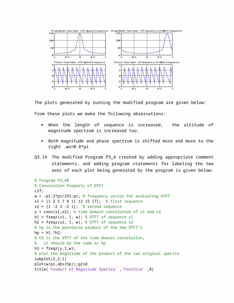
Q3.13 Program P3_3 was run for the following values of the frequency-shift: 0.8*pi and for the following values of length for the sequence: 12

-1 -0.5 0 0.5 10
50
100
150Magnitude Spectrum of Original Sequence
-1 -0.5 0 0.5 10
50
100
150Magnitude Spectrum of Frequency-Shifted Sequence
-1 -0.5 0 0.5 1-4
-2
0
2
4Phase Spectrum of Original Sequence
-1 -0.5 0 0.5 1-4
-2
0
2
4Phase Spectrum of Frequency-Shifted Sequence
The plots generated by running the modified program are given below:
From these plots we make the following observations:
When the length of sequence is increased, the altitude of magnitude spectrum is increased too.
Both magnitude and phase spectrum is shifted more and more to the right .wo=0.8*pi
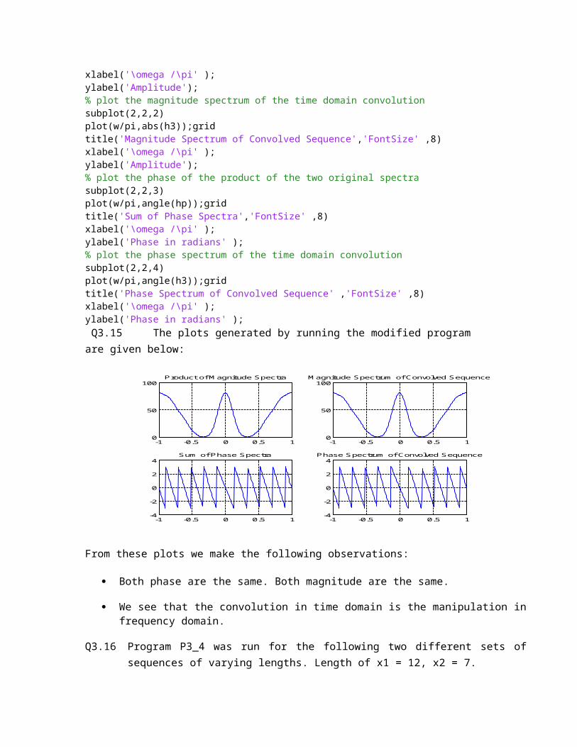
Q3.14 The modified Program P3_4 created by adding appropriate comment statements, and adding program statements for labeling the two axes of each plot being generated by the program is given below:
% Program P3_4B % Convolution Property of DTFT clf; w = -pi:2*pi/255:pi; % frequency vector for evaluating DTFT x1 = [1 3 5 7 9 11 13 15 17]; % first sequence x2 = [1 -2 3 -2 1]; % second sequence y = conv(x1,x2); % time domain convolution of x1 and x2 h1 = freqz(x1, 1, w); % DTFT of sequence x1 h2 = freqz(x2, 1, w); % DTFT of sequence x2 % hp is the pointwise product of the two DTFT's hp = h1.*h2; % h3 is the DTFT of the time domain convolution; % it should be the same as hp h3 = freqz(y,1,w); % plot the magnitude of the product of the two original spectra subplot(2,2,1) plot(w/pi,abs(hp));grid title('Product of Magnitude Spectra' ,'FontSize' ,8) xlabel('\omega /\pi' ); ylabel('Amplitude'); % plot the magnitude spectrum of the time domain convolution subplot(2,2,2) plot(w/pi,abs(h3));grid title('Magnitude Spectrum of Convolved Sequence','FontSize' ,8) xlabel('\omega /\pi' ); ylabel('Amplitude');
% plot the phase of the product of the two original spectrasubplot(2,2,3) plot(w/pi,angle(hp));grid title('Sum of Phase Spectra','FontSize' ,8) xlabel('\omega /\pi' ); ylabel('Phase in radians' ); % plot the phase spectrum of the time domain convolution subplot(2,2,4) plot(w/pi,angle(h3));grid title('Phase Spectrum of Convolved Sequence' ,'FontSize' ,8) xlabel('\omega /\pi' ); ylabel('Phase in radians' ); Q3.15 The plots generated by running the modified program are given below:
-1 -0.5 0 0.5 10
50
100Product of Magnitude Spectra
-1 -0.5 0 0.5 10
50
100Magnitude Spectrum of Convolved Sequence
-1 -0.5 0 0.5 1-4
-2
0
2
4Sum of Phase Spectra
-1 -0.5 0 0.5 1-4
-2
0
2
4Phase Spectrum of Convolved Sequence
From these plots we make the following observations:
Both phase are the same. Both magnitude are the same.
We see that the convolution in time domain is the manipulation in frequency domain.
Q3.16 Program P3_4 was run for the following two different sets of sequences of varying lengths. Length of x1 = 12, x2 = 7.
x1 = [1 3 5 7 9 11 13 15 17 19 21 23 ];
x2 = [1 -2 3 -2 1 3 4];
-1 -0.5 0 0.5 10
500
1000
1500Product of Magnitude Spectra
-1 -0.5 0 0.5 10
500
1000
1500Magnitude Spectrum of Convolved Sequence
-1 -0.5 0 0.5 1-4
-2
0
2
4Sum of Phase Spectra
-1 -0.5 0 0.5 1-4
-2
0
2
4Phase Spectrum of Convolved Sequence
The plots generated by running the modified program are given below:
When the length changes, the properties discovered in Q3.16 doesn’t change. Both phase are the same. Both magnitude are the same.
Q3.17 The modified Program P3_5 created by adding appropriate comment statements, and adding program statements for labeling the two axes of each plot being generated by the program is given below:
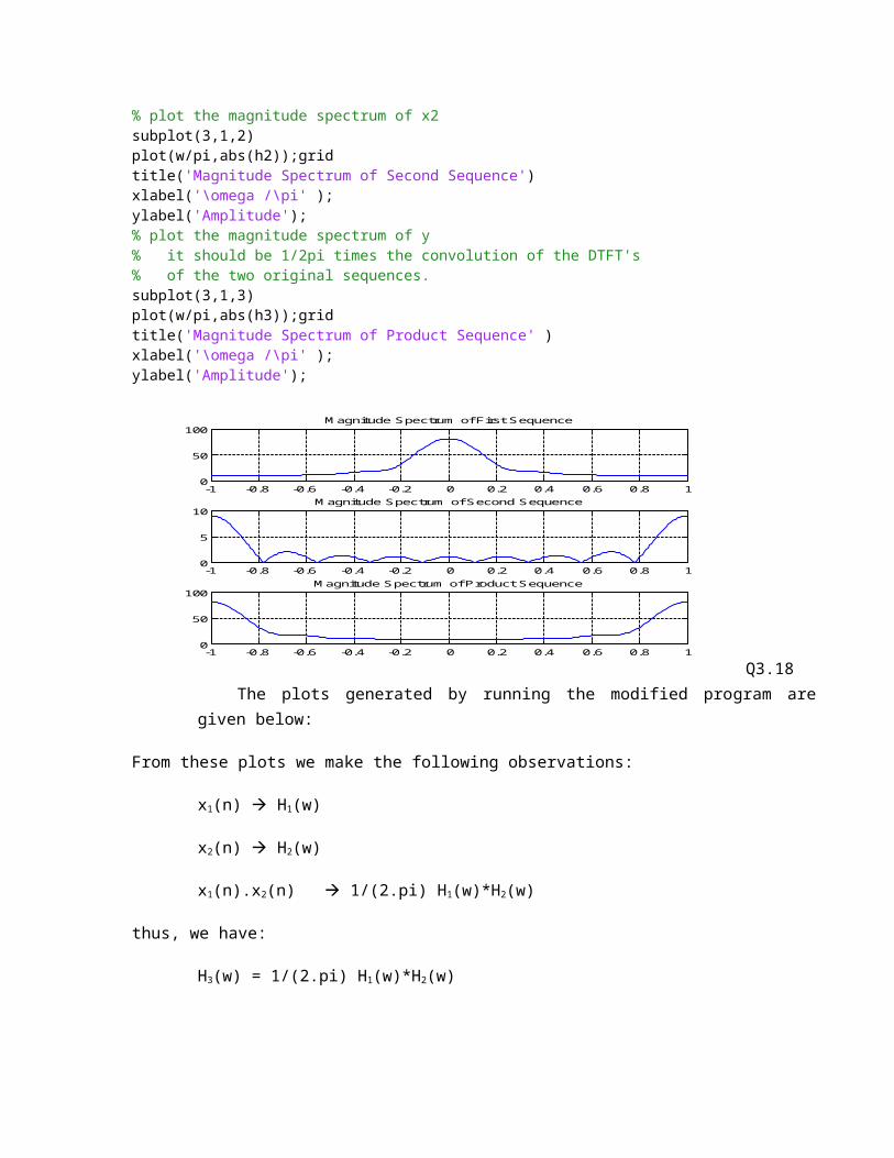
% Program P3_5B % Modulation Property of DTFT clf; w = -pi:2*pi/255:pi; % freqency vector for evaluating DTFT x1 = [1 3 5 7 9 11 13 15 17]; % first sequence x2 = [1 -1 1 -1 1 -1 1 -1 1]; % second sequence % y is the time domain pointwise product of x1 and x2 y = x1.*x2; h1 = freqz(x1, 1, w); % DTFT of sequence x1 h2 = freqz(x2, 1, w); % DTFT of sequence x2 h3 = freqz(y,1,w); % DTFT of sequence y % plot the magnitude spectrum of x1 subplot(3,1,1) plot(w/pi,abs(h1));grid title('Magnitude Spectrum of First Sequence' ) xlabel('\omega /\pi' ); ylabel('Amplitude'); % plot the magnitude spectrum of x2 subplot(3,1,2) plot(w/pi,abs(h2));grid title('Magnitude Spectrum of Second Sequence') xlabel('\omega /\pi' ); ylabel('Amplitude'); % plot the magnitude spectrum of y % it should be 1/2pi times the convolution of the DTFT's % of the two original sequences. subplot(3,1,3) plot(w/pi,abs(h3));grid title('Magnitude Spectrum of Product Sequence' )

xlabel('\omega /\pi' ); ylabel('Amplitude');
-1 -0.8 -0.6 -0.4 -0.2 0 0.2 0.4 0.6 0.8 10
50
100Magnitude Spectrum of First Sequence
-1 -0.8 -0.6 -0.4 -0.2 0 0.2 0.4 0.6 0.8 10
5
10Magnitude Spectrum of Second Sequence
-1 -0.8 -0.6 -0.4 -0.2 0 0.2 0.4 0.6 0.8 10
50
100Magnitude Spectrum of Product Sequence
Q3.18 The plots generated by running the modified program are given below:
From these plots we make the following observations:
x1(n) H1(w)
x2(n) H2(w)
x1(n).x2(n) 1/(2.pi) H1(w)*H2(w)
thus, we have:
H3(w) = 1/(2.pi) H1(w)*H2(w)
Q3.19 Program P3_5 was run for the following two different sets of sequences of varying lengths:
x1 = [1 3 5 7 9 11 13 15 17 19 21 23 25]
x2 = [1 -1 1 -1 1 -1 1 -1 1 -1 1 -1 1]
The plots generated by running the modified program are given below:
-1 -0.8 -0.6 -0.4 -0.2 0 0.2 0.4 0.6 0.8 10
100
200Magnitude Spectrum of First Sequence
-1 -0.8 -0.6 -0.4 -0.2 0 0.2 0.4 0.6 0.8 10
10
20Magnitude Spectrum of Second Sequence
-1 -0.8 -0.6 -0.4 -0.2 0 0.2 0.4 0.6 0.8 10
100
200Magnitude Spectrum of Product Sequence
From these plots we make the following observations: When the length changes, modulation property dosen’t change.
Q3.20 The modified Program P3_6 created by adding appropriate comment statements, and adding program statements for labeling the two axes of each plot being generated by the program is given below:
% Program P3_6
% Program P3_6B % Time Reversal Property of DTFT clf; w = -pi:2*pi/255:pi; % freqency vector for evaluating DTFT % original ramp sequence % note: num is nonzero for 0 <= n <= 3. num = [1 2 3 4]; L = length(num)-1; h1 = freqz(num, 1, w); % DTFT of original ramp sequence h2 = freqz(fliplr(num), 1, w); h3 = exp(w*L*i).*h2; % plot the magnitude spectrum of the original ramp sequence subplot(2,2,1) plot(w/pi,abs(h1));grid title('Magnitude Spectrum of Original Sequence','FontSize' ,8) xlabel('\omega /\pi' ); ylabel('Amplitude'); % plot the magnitude spectrum of the time reversed ramp sequence subplot(2,2,2) plot(w/pi,abs(h3));grid title('Magnitude Spectrum of Time-Reversed Sequence','FontSize' ,8) xlabel('\omega /\pi' ); ylabel('Amplitude'); % plot the phase spectrum of the original ramp sequence subplot(2,2,3) plot(w/pi,angle(h1));grid title('Phase Spectrum of Original Sequence','FontSize' ,8) xlabel('\omega /\pi' ); ylabel('Phase in radians' );

% plot the phase spectrum of the time reversed ramp sequence subplot(2,2,4) plot(w/pi,angle(h3));grid title('Phase Spectrum of Time-Reversed Sequence','FontSize' ,8) xlabel('\omega /\pi' ); ylabel('Phase in radians' );
The program implements the time-reversal operation as follows :
A new sequence is formed by using fliplr this new sequence contains the samples of the original ramp sequence in time reversed order
h2 = freqz(fliplr(num), 1, w);
h3 = exp(w*L*i).*h2;
Q3.21 The plots generated by running the modified program are given below:
-1 -0.5 0 0.5 12
4
6
8
10Magnitude Spectrum of Original Sequence
w
A
-1 -0.5 0 0.5 12
4
6
8
10Magnitude Spectrum of Time-Reversed Sequence
w
A
-1 -0.5 0 0.5 1-4
-2
0
2
4Phase Spectrum of Original Sequence
w
Phase
-1 -0.5 0 0.5 1-4
-2
0
2
4Phase Spectrum of Time-Reversed Sequence
w
Phase
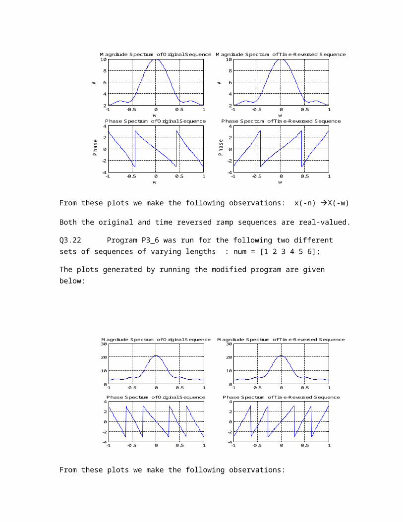
From these plots we make the following observations: x(-n) X(-w)
Both the original and time reversed ramp sequences are real-valued.
Q3.22 Program P3_6 was run for the following two different sets of sequences of varying lengths : num = [1 2 3 4 5 6];
The plots generated by running the modified program are given below:

-1 -0.5 0 0.5 10
10
20
30Magnitude Spectrum of Original Sequence
-1 -0.5 0 0.5 10
10
20
30Magnitude Spectrum of Time-Reversed Sequence
-1 -0.5 0 0.5 1-4
-2
0
2
4Phase Spectrum of Original Sequence
-1 -0.5 0 0.5 1-4
-2
0
2
4Phase Spectrum of Time-Reversed Sequence
From these plots we make the following observations:
Both the original and time reversed ramp sequences are real-valued.
3.2 DISCRETE FOURIER TRANSFORM
Project 3.3 DFT and IDFT Computations
Answers:
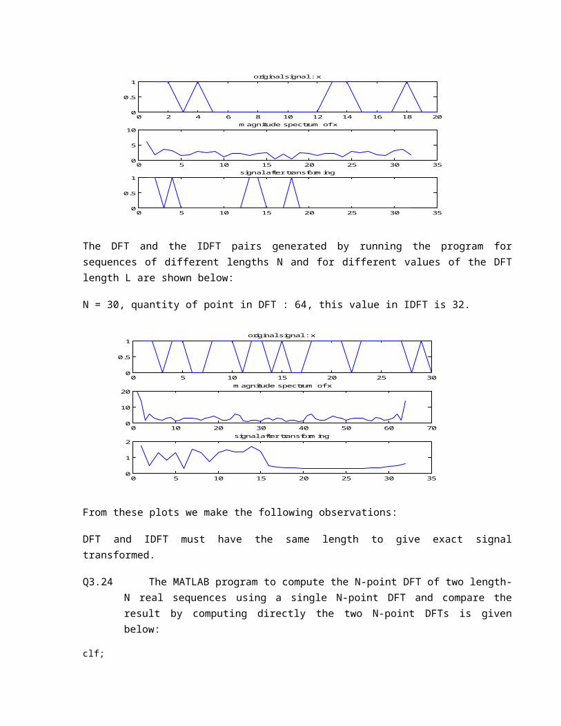
Q3.23 The MATLAB program to compute and plot the L-point DFT X[k] of a length-N sequence x[n] with L N and then to compute and plot the IDFT of X[k] is given below:
clf;
clc;
N=20;
x=randint(1,N);
subplot(3,1,1)
plot(x);
title('original signal : x');
y=fft(x,32);
subplot(3,1,2)
plot(abs(y));
title(' magnitude spectrum of x');
ix=ifft(y,32);
subplot(3,1,3)
plot(abs(ix));
title('signal after transforming')
Figure
0 2 4 6 8 10 12 14 16 18 200
0.5
1original signal : x
0 5 10 15 20 25 30 350
5
10 magnitude spectrum of x
0 5 10 15 20 25 30 350
0.5
1signal after transforming
The DFT and the IDFT pairs generated by running the program for sequences of different lengths N and for different values of the DFT length L are shown below:
N = 30, quantity of point in DFT : 64, this value in IDFT is 32.
0 5 10 15 20 25 300
0.5
1original signal : x
0 10 20 30 40 50 60 700
10
20 magnitude spectrum of x
0 5 10 15 20 25 30 350
1
2signal after transforming
From these plots we make the following observations:
DFT and IDFT must have the same length to give exact signal transformed.

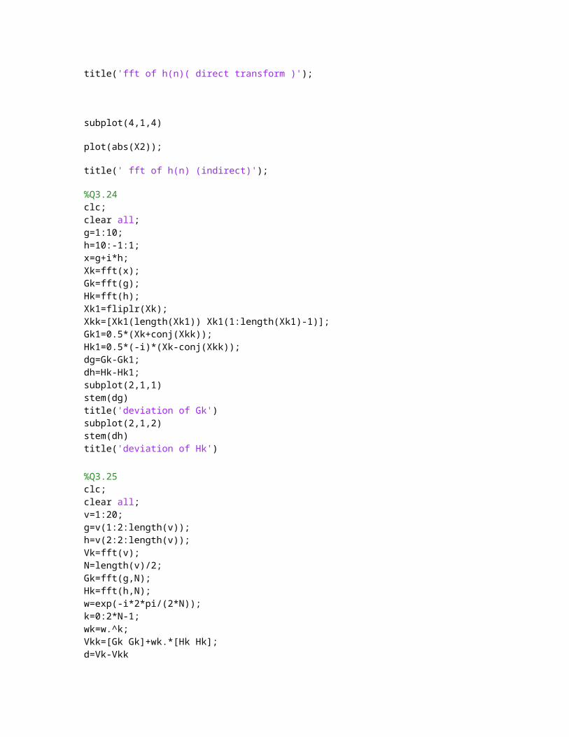
Q3.24 The MATLAB program to compute the N-point DFT of two length-N real sequences using a single N-point DFT and compare the result by computing directly the two N-point DFTs is given below:
clf;
clc;
N=30;
x1=randint(1,N);
x2=randint(1,N);
x=x1+i*x2;
X=fft(x,64);
dX1=fft(x1,64);
dX2=fft(x2,64);
Xcon=conj(X);
Xconf=[Xcon(1) fliplr(X(2:length(Xcon)))];
X1=0.5*(X + Xconf);
X2=(0.5/i)*(X - Xconf);
subplot(4,1,1)
plot(abs(dX1));
title('fft of g(n)( direct transform )');
subplot(4,1,2)
plot(abs(X1));
title(' fft of g(n) (indirect)');
subplot(4,1,3)
plot(abs(dX2));
title('fft of h(n)( direct transform )');
subplot(4,1,4)
plot(abs(X2));
title(' fft of h(n) (indirect)');
%Q3.24clc;clear all;g=1:10;h=10:-1:1;x=g+i*h;Xk=fft(x);Gk=fft(g);Hk=fft(h);Xk1=fliplr(Xk);Xkk=[Xk1(length(Xk1)) Xk1(1:length(Xk1)-1)];Gk1=0.5*(Xk+conj(Xkk));Hk1=0.5*(-i)*(Xk-conj(Xkk));dg=Gk-Gk1;dh=Hk-Hk1;subplot(2,1,1)stem(dg)title('deviation of Gk')subplot(2,1,2)stem(dh)title('deviation of Hk')
%Q3.25clc;clear all;v=1:20;g=v(1:2:length(v));h=v(2:2:length(v));Vk=fft(v);N=length(v)/2;Gk=fft(g,N);Hk=fft(h,N);w=exp(-i*2*pi/(2*N));k=0:2*N-1;wk=w.^k;Vkk=[Gk Gk]+wk.*[Hk Hk];d=Vk-Vkksubplot(3,1,1)stem(Vkk)title('2N-point DFT')subplot(3,1,2)stem(Vk)title('N-point DFT')subplot(3,1,3)stem(d)title('deviation')

The DFTs generated by running the program for sequences of different lengths N are shown below:
0 10 20 30 40 50 60 700
10
20fft of g(n)( direct transform )
0 10 20 30 40 50 60 700
10
20 fft of g(n) (indirect)
0 10 20 30 40 50 60 700
10
20fft of h(n)( direct transform )
0 10 20 30 40 50 60 700
10
20 fft of h(n) (indirect)
From these plots we make the following observations: between direct and indirect the transform is nearly the same.
Project 3.4 DFT Properties
Answers:
Q3.26 The purpose of the command rem in the function circshift is used to give us the remainder of division.
Q3.27 The function circshift operates as follows :
Array will be shifted in circular by M samples.
Q3.28 The purpose of the operator ~= in the function circonv is used to compare two objects. This is the binary relational NOT EQUAL operator.
Q3.29 The function circonv operates as follows:
This function computate convolution in circle.
Q3.30 The modified Program P3_7 created by adding appropriate comment statements, and adding program statements for labeling each plot being generated by the program is given below:
% Program P3_7B % Illustration of Circular Shift of a Sequence clf; % initialize shift amount M M = 6; % initialize sequence a to be shifted a = [0 1 2 3 4 5 6 7 8 9]; b = circshift(a,M); % perform the circular shift L = length(a)-1; % plot the original sequence a and the circularly shifted sequence b n = 0:L; subplot(2,1,1); stem(n,a);axis([0,L,min(a),max(a)]); title('Original Sequence'); xlabel('time index n'); ylabel('a[n]'); subplot(2,1,2); stem(n,b);axis([0,L,min(a),max(a)]); title(['Sequence Obtained by Circularly Shifting by ',num2str(M),' Samples' ]); xlabel('time index n'); ylabel('b[n]');
The parameter determining the amount of time-shifting is M.
If the amount of time-shift is greater than the sequence length then M = rem(M,length(x));
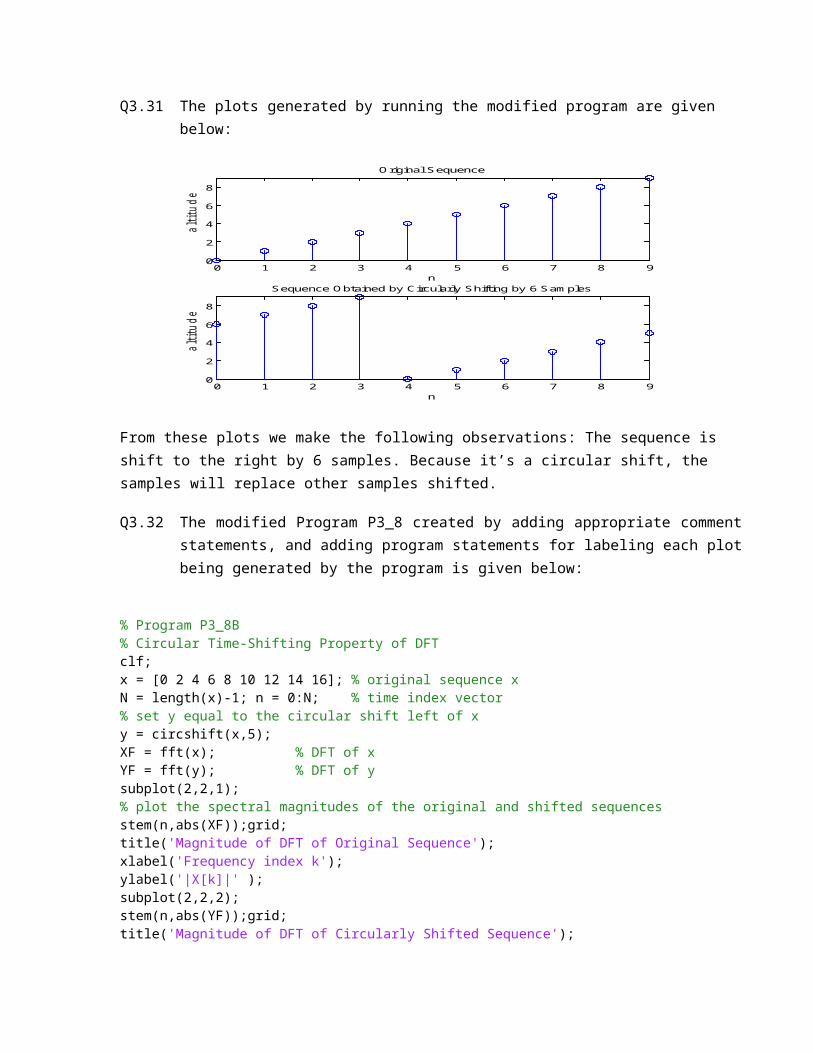
Q3.31 The plots generated by running the modified program are given below:
0 1 2 3 4 5 6 7 8 90
2
4
6
8
Original Sequence
n
altitude
0 1 2 3 4 5 6 7 8 90
2
4
6
8
Sequence Obtained by Circularly Shifting by 6 Samples
n
altitude
From these plots we make the following observations: The sequence is shift to the right by 6 samples. Because it’s a circular shift, the samples will replace other samples shifted.
Q3.32 The modified Program P3_8 created by adding appropriate comment statements, and adding program statements for labeling each plot being generated by the program is given below:

% Program P3_8B % Circular Time-Shifting Property of DFT clf; x = [0 2 4 6 8 10 12 14 16]; % original sequence x N = length(x)-1; n = 0:N; % time index vector % set y equal to the circular shift left of x y = circshift(x,5); XF = fft(x); % DFT of x YF = fft(y); % DFT of y subplot(2,2,1); % plot the spectral magnitudes of the original and shifted sequences stem(n,abs(XF));grid; title('Magnitude of DFT of Original Sequence'); xlabel('Frequency index k'); ylabel('|X[k]|' ); subplot(2,2,2); stem(n,abs(YF));grid; title('Magnitude of DFT of Circularly Shifted Sequence'); xlabel('Frequency index k'); ylabel('|Y[k]|' ); % plot the spectral phases of the original and shifted sequences subplot(2,2,3); stem(n,angle(XF));grid; title('Phase of DFT of Original Sequence' ); xlabel('Frequency index k'); ylabel('arg(X[k])'); subplot(2,2,4); stem(n,angle(YF));grid; title('Phase of DFT of Circularly Shifted Sequence' ); xlabel('Frequency index k'); ylabel('arg(Y[k])');
The amount of time-shift is 5
Q3.33 The plots generated by running the modified program are given below:
0 2 4 6 80
20
40
60
80Magnitude of DFT of Original Sequence
0 2 4 6 80
20
40
60
80Magnitude of DFT of Circularly Shifted Sequence
0 2 4 6 8-4
-2
0
2
4Phase of DFT of Original Sequence
0 2 4 6 8-4
-2
0
2
4Phase of DFT of Circularly Shifted Sequence

From these plots we make the following observations:
The altitude is not changed when sequence is shifted.
The phase is changed with rule:
x(n) X(k)
x(n-n0) X(k).exp (-j2πkn0/N)
Q3.34 The plots generated by running the modified program for the following two different amounts of time-shifts, with the amount of shift indicated, are shown below:
When time-shift = 7, we have
0 2 4 6 80
20
40
60
80Magnitude of DFT of Original Sequence
Altitude (
V)
w 0 2 4 6 8
0
20
40
60
80Magnitude of DFT of Circularly Shifted Sequence
Altitude (
V)
w
0 2 4 6 8-4
-2
0
2
4Phase of DFT of Original Sequence
Phase
w 0 2 4 6 8
-4
-2
0
2
4Phase of DFT of Circularly Shifted Sequence
Phase
w
when time-shift = 10 , we have
0 2 4 6 80
20
40
60
80Magnitude of DFT of Original Sequence
Altitude (
V)
w 0 2 4 6 8
0
20
40
60
80Magnitude of DFT of Circularly Shifted Sequence
Altitude (
V)
w
0 2 4 6 8-4
-2
0
2
4Phase of DFT of Original Sequence
Phase
w 0 2 4 6 8
-4
-2
0
2
4Phase of DFT of Circularly Shifted Sequence
Phase
w
From these plots we make the following observations: When time-shift is changed, we observe that only the phase of shifted sequence is changed.
Q3.35 The plots generated by running the modified program for the following two different sequences of different lengths, with the lengths indicated, are shown below:
When :
x = [0 2 4 6 8 10 12 14 16 18 20 22];
0 5 10 150
50
100
150Magnitude of DFT of Original Sequence
Altitude (
V)
w 0 5 10 15
0
50
100
150Magnitude of DFT of Circularly Shifted Sequence
Altitude (
V)
w
0 5 10 15-4
-2
0
2
4Phase of DFT of Original Sequence
Phase
w 0 5 10 15
-4
-2
0
2
4Phase of DFT of Circularly Shifted Sequence
Phase
w
When:
x = [0 2 4 6 8 10 12 14 16 18 20 22 24 26 28 16];
From these plots we make the following observations:
0 5 10 150
100
200
300Magnitude of DFT of Original Sequence
Altitude (
V)
w 0 5 10 15
0
100
200
300Magnitude of DFT of Circularly Shifted Sequence
Altitude (
V)
w
0 5 10 15-4
-2
0
2
4Phase of DFT of Original Sequence
Phase
w 0 5 10 15
-4
-2
0
2
4Phase of DFT of Circularly Shifted Sequence
Phase
w

When the length of sequence changes, the magnitude changes but the original sequence and the shifted signal are the same.
The phase changes.
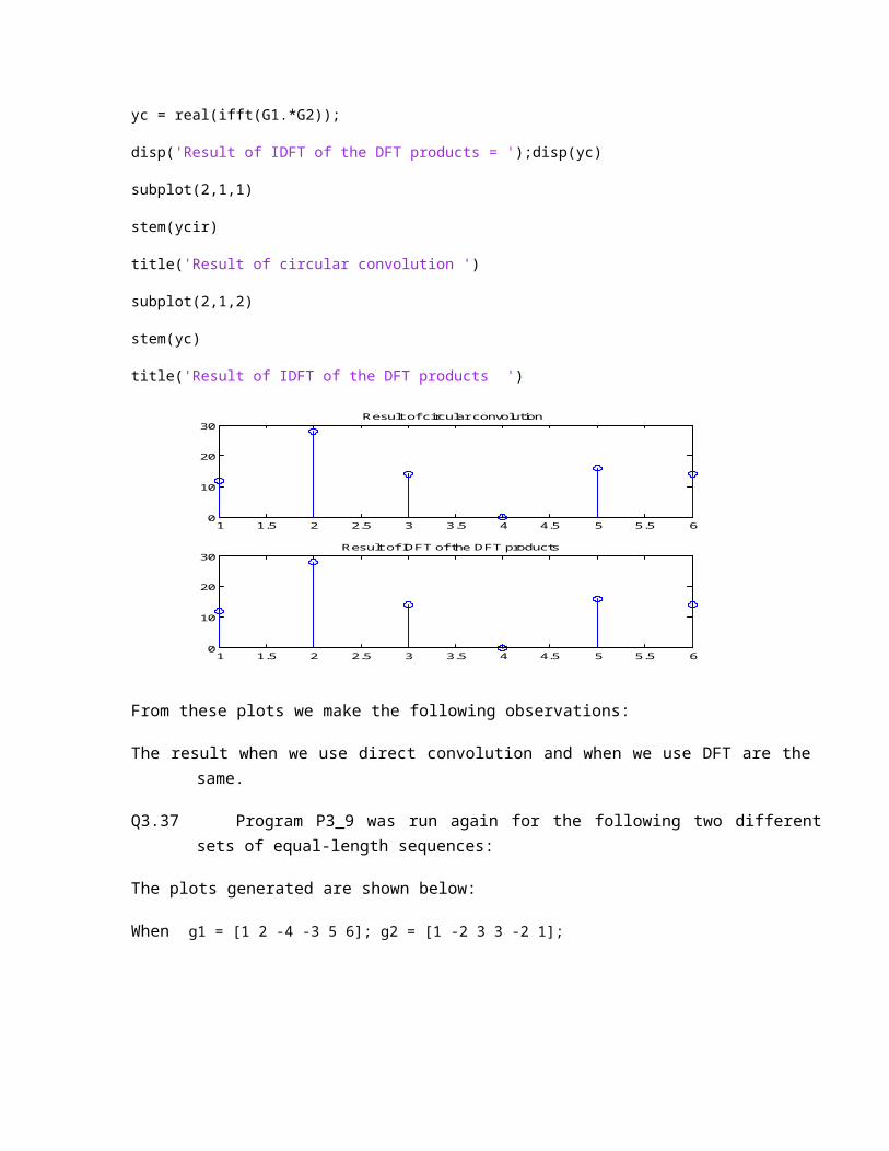
Q3.36 A copy of Program P3_9 is given below along with the plots generated by running this program:
% Program P3_9
% Circular Convolution Property of DFT
g1 = [1 2 3 4 5 6]; g2 = [1 -2 3 3 -2 1];
ycir = Circonv(g1,g2);
disp('Result of circular convolution = ');disp(ycir)
G1 = fft(g1); G2 = fft(g2);
yc = real(ifft(G1.*G2));
disp('Result of IDFT of the DFT products = ');disp(yc)
Result of circular convolution =
12 28 14 0 16 14
Result of IDFT of the DFT products =
12 28 14 0 16 14
the modified P3_9 to show figure is:
% q3.36
% Circular Convolution Property of DFT
g1 = [1 2 3 4 5 6]; g2 = [1 -2 3 3 -2 1];
ycir = Circonv(g1,g2);
disp('Result of circular convolution = ');disp(ycir)
G1 = fft(g1); G2 = fft(g2);
yc = real(ifft(G1.*G2));
disp('Result of IDFT of the DFT products = ');disp(yc)
subplot(2,1,1)

stem(ycir)
title('Result of circular convolution ')
subplot(2,1,2)
stem(yc)
title('Result of IDFT of the DFT products ')
1 1.5 2 2.5 3 3.5 4 4.5 5 5.5 60
10
20
30Result of circular convolution
1 1.5 2 2.5 3 3.5 4 4.5 5 5.5 60
10
20
30Result of IDFT of the DFT products
From these plots we make the following observations:
The result when we use direct convolution and when we use DFT are the same.
Q3.37 Program P3_9 was run again for the following two different sets of equal-length sequences:
The plots generated are shown below:
When g1 = [1 2 -4 -3 5 6]; g2 = [1 -2 3 3 -2 1];
1 1.5 2 2.5 3 3.5 4 4.5 5 5.5 6-40
-20
0
20
40Result of circular convolution
1 1.5 2 2.5 3 3.5 4 4.5 5 5.5 6-40
-20
0
20
40Result of IDFT of the DFT products

When g1 = [1 2 -4 -3 5 6 3]; g2 = [1 -2 3 3 -2 1 4];
1 2 3 4 5 6 7-20
0
20
40Result of circular convolution
1 2 3 4 5 6 7-20
0
20
40Result of IDFT of the DFT products
From these plots we make the following observations:
Although the elements of sequence get different value or different length, the result when we change method are the same.
Q3.38 A copy of Program P3_10 is given below along with the plots generated by running this program:
% Program P3_10
% Linear Convolution via Circular Convolution
g1 = [1 2 3 4 5];g2 = [2 2 0 1 1];
g1e = [g1 zeros(1,length(g2)-1)];
g2e = [g2 zeros(1,length(g1)-1)];
ylin = circonv(g1e,g2e);
disp('Linear convolution via circular convolution = ');disp(ylin);
y = conv(g1, g2);
disp('Direct linear convolution = ');disp(y)
The modified program

% Modified Program P3_10 to show figure
% Linear Convolution via Circular Convolution
g1 = [1 2 3 4 5];g2 = [2 2 0 1 1];
g1e = [g1 zeros(1,length(g2)-1)];
g2e = [g2 zeros(1,length(g1)-1)];
ylin = circonv(g1e,g2e);
disp('Linear convolution via circular convolution = ');disp(ylin);
y = conv(g1, g2);
disp('Direct linear convolution = ');disp(y)
subplot(2,1,1)
stem(ylin)
title('Circular convolution')
subplot(2,1,2)
stem(y)
title('Linear convolution')
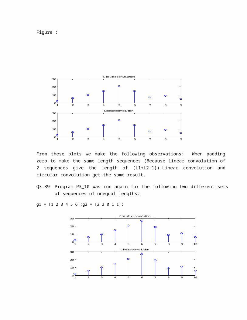
Figure :
1 2 3 4 5 6 7 8 90
10
20
30Circular convolution
1 2 3 4 5 6 7 8 90
10
20
30Linear convolution
From these plots we make the following observations: When padding zero to make the same length sequences (Because linear convolution of 2 sequences give the length of (L1+L2-1)).Linear convolution and circular convolution get the same result.
Q3.39 Program P3_10 was run again for the following two different sets of sequences of unequal lengths:
g1 = [1 2 3 4 5 6];g2 = [2 2 0 1 1];
1 2 3 4 5 6 7 8 9 100
10
20
30Circular convolution
1 2 3 4 5 6 7 8 9 100
10
20
30Linear convolution
g1 = [1 2 3 4 5 6];g2 = [2 2 0 1 1 7 8];
0 2 4 6 8 10 120
50
100Circular convolution
0 2 4 6 8 10 120
50
100Linear convolution
From these plots we make the following observations: When length of sequences are different, the convolution is the same.
Q3.40 The MATLAB program to develop the linear convolution of two sequences via the DFT of each is given below:
% Linear Convolution via the DFT
g1 = [1 2 3 4 5];g2 = [2 2 0 1 1];

y = conv(g1, g2);
g1e = [g1 zeros(1,length(g2)-1)];
g2e = [g2 zeros(1,length(g1)-1)];
G1 = fft(g1e); G2 = fft(g2e);
yc = real(ifft(G1.*G2));
subplot(2,1,1)
stem(y)
title('Sequence (Direct linear convolution)')
subplot(2,1,2)
stem(yc)
title(' Sequence (Using DFT)')
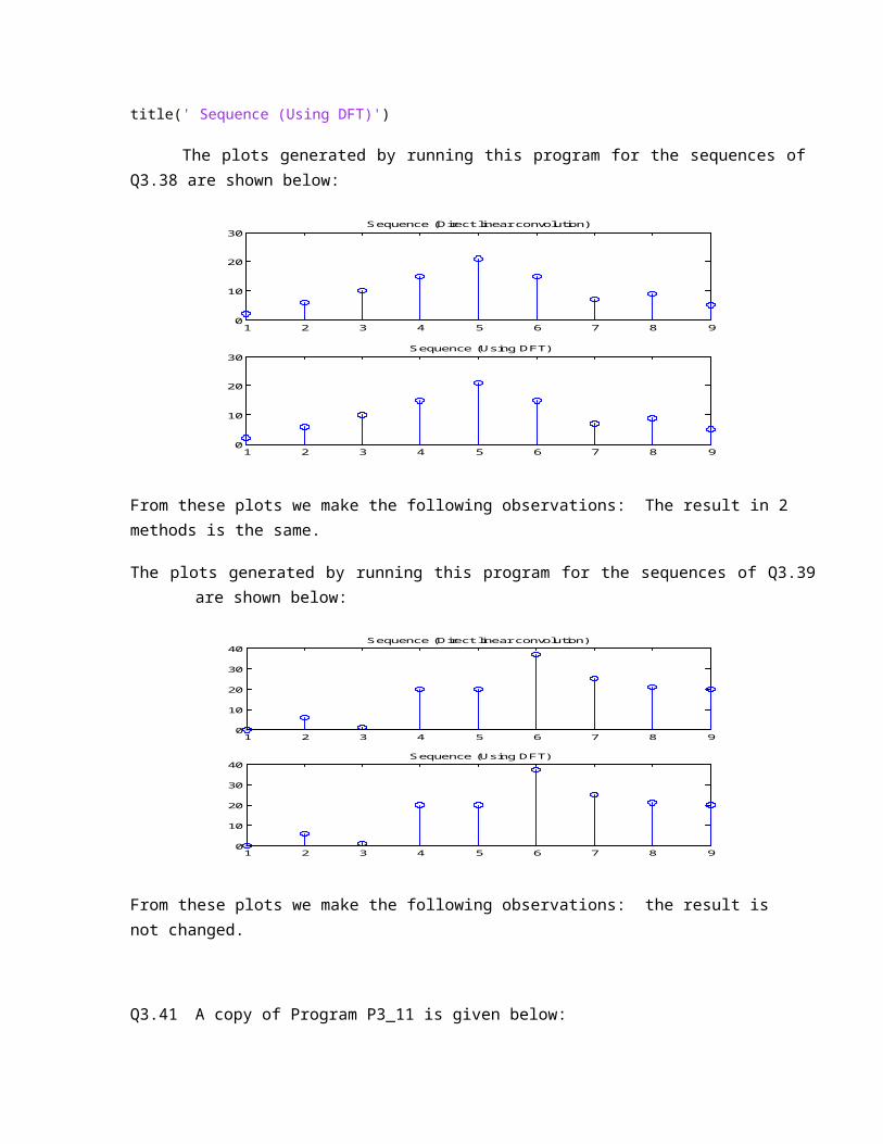
The plots generated by running this program for the sequences of Q3.38 are shown below:
1 2 3 4 5 6 7 8 90
10
20
30Sequence (Direct linear convolution)
1 2 3 4 5 6 7 8 90
10
20
30 Sequence (Using DFT)
From these plots we make the following observations: The result in 2 methods is the same.
The plots generated by running this program for the sequences of Q3.39 are shown below:

1 2 3 4 5 6 7 8 90
10
20
30
40Sequence (Direct linear convolution)
1 2 3 4 5 6 7 8 90
10
20
30
40 Sequence (Using DFT)
From these plots we make the following observations: the result is not changed.
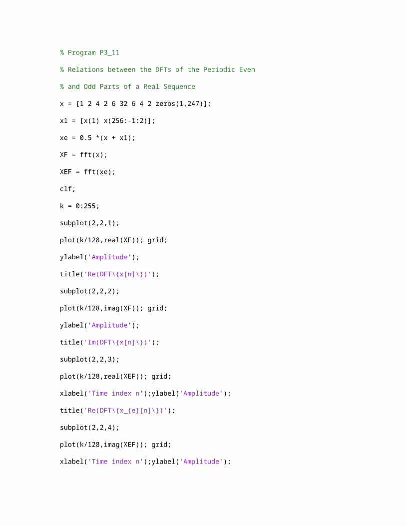
Q3.41 A copy of Program P3_11 is given below:
% Program P3_11
% Relations between the DFTs of the Periodic Even
% and Odd Parts of a Real Sequence
x = [1 2 4 2 6 32 6 4 2 zeros(1,247)];
x1 = [x(1) x(256:-1:2)];
xe = 0.5 *(x + x1);
XF = fft(x);
XEF = fft(xe);
clf;
k = 0:255;
subplot(2,2,1);
plot(k/128,real(XF)); grid;
ylabel('Amplitude');
title('Re(DFT\{x[n]\})');
subplot(2,2,2);
plot(k/128,imag(XF)); grid;
ylabel('Amplitude');
title('Im(DFT\{x[n]\})');
subplot(2,2,3);
plot(k/128,real(XEF)); grid;
xlabel('Time index n');ylabel('Amplitude');
title('Re(DFT\{x_{e}[n]\})');
subplot(2,2,4);
plot(k/128,imag(XEF)); grid;
xlabel('Time index n');ylabel('Amplitude');
title('Im(DFT\{x_{e}[n]\})');
The relation between the sequence x1[n] and x[n] is x1[n] = x[-n].
Q3.42 The plots generated by running Program P3_11 are given below:
0 0.5 1 1.5 2-50
0
50
100
Am
plitu
de
Re(DFT{x[n]})
0 0.5 1 1.5 2-100
-50
0
50
100
Am
plitu
de
Im(DFT{x[n]})
0 0.5 1 1.5 2-50
0
50
100
Time index n
Am
plitu
de
Re(DFT{xe[n]})
0 0.5 1 1.5 2
-0.5
0
0.5
x 10-14
Time index n
Am
plitu
de
Im(DFT{xe[n]})
The imaginary part of XEF is equal to zero. This result can be explained as follows:
xe(n) = ½(x(n) + x(-n))
If X(k) is the N-point DFT of x(n), the N-point DFT of xe(n) is the real part of X(k), so Re(DFT(xe(n))) is the same of Re(DFT(x(n))).
Q3.43 The required modifications to Program P3_11 to verify the relation between the DFT of the periodic odd part and the imaginary part of XEF are given below along with the plots generated by running this program:

% Relations between the DFTs of the Periodic Odd part
% and the imaginary part of XEF
x = [1 2 4 2 6 32 6 4 2 zeros(1,247)];
x1 = [x(1) x(256:-1:2)];
xe = 0.5 *(x + x1);
xo = 0.5 *(x - x1);
XEF = fft(xe);
XOF = fft(xo);
clf;
k = 0:255;
subplot(2,2,1);
plot(k/128,real(XOF)); grid;
ylabel('Amplitude');
title('Re(DFT\{x_{o}[n]\})');
subplot(2,2,2);
plot(k/128,imag(XOF)); grid;
ylabel('Amplitude');
title('Im(DFT\{x_{o}[n]\})');
subplot(2,2,3);
plot(k/128,real(XEF)); grid;
xlabel('Time index n');ylabel('Amplitude');
title('Re(DFT\{x_{e}[n]\})');
subplot(2,2,4);
plot(k/128,imag(XEF)); grid;
xlabel('Time index n');ylabel('Amplitude');
title('Im(DFT\{x_{e}[n]\})');
0 0.5 1 1.5 2
-0.5
0
0.5
x 10-14
Am
plitu
de
Re(DFT{xo[n]})
0 0.5 1 1.5 2-100
-50
0
50
100
Am
plitu
de
Im(DFT{xo[n]})
0 0.5 1 1.5 2-50
0
50
100
Time index n
Am
plitu
de
Re(DFT{xe[n]})
0 0.5 1 1.5 2
-0.5
0
0.5
x 10-14
Time index n
Am
plitu
de
Im(DFT{xe[n]})
From these plots we make the following observations:
xo(n) = ½(x(n) - x(-n))
N-points DFT of xo(n) is the imaginary part of x(n). The imaginar part of XOF is unequal to zero, whereas the imaginary part of XEF is nearly zero.
Q3.44 A copy of Program P3_12 is given below:
% Program P3_12
% Parseval's Relation
x = [(1:128) (128:-1:1)];
XF = fft(x);
a = sum(x.*x)
b = round(sum(abs(XF).^2)/256)
The values for a and b we get by running this program are
a = 1414528
b = 1414528
Q3.45 The required modifications to Program P3_11 are given below:
% Modified Program P3_12
% Parseval's Relation
clc;
x = [(1:128) (128:-1:1)];
XF = fft(x);
a = sum(x.*x)
absXF=XF.*conj(XF);
b = round(sum(absXF)/256)
We have the same result as in Q3.44.
3.3 z-TRANSFORM
Project 3.5 Analysis of z-Transforms
Answers:
Q3.46 The frequency response of the z-transform obtained using Program P3_1 is plotted below:
With the the z-transform:
G( z )=2+5 z−1+9 z−2+5 z−3+3 z−4
5+45 z−1+2 z−2+z−3+z−4
Code
% q346
% Evaluation of the z-transform
clf;
w = -4*pi:8*pi/511:4*pi;
num = [2 5 9 5 3];den = [5 45 2 1 1];
h = freqz(num, den, w);
subplot(2,1,1)
plot(w/pi,abs(h));grid
title('Magnitude Spectrum')
xlabel('\omega /\pi');
ylabel('Amplitude');

subplot(2,1,2)
plot(w/pi,angle(h));grid
title('Phase Spectrum')
xlabel('\omega /\pi');
ylabel('Phase in radians')
-4 -3 -2 -1 0 1 2 3 40
0.2
0.4
0.6
0.8Magnitude Spectrum
/
Am
plitude
-4 -3 -2 -1 0 1 2 3 4-4
-2
0
2
4Phase Spectrum
/
Phase in
radia
ns
Q3.47 The MATLAB program to compute and display the poles and zeros, to compute and display the factored form, and to generate the pole-zero plot of a rational z-transform is given below:
clc;
w = -4*pi:8*pi/511:4*pi;
num = [2 5 9 5 3];den = [5 45 2 1 1];%q3.47
zplane(num,den)
[z,p,k]=tf2zp(num,den);
disp('zeros')
disp(z);
disp('poles')
disp(p);

-9 -8 -7 -6 -5 -4 -3 -2 -1 0 1
-4
-3
-2
-1
0
1
2
3
4
Real Part
Imagin
ary
Part
zeros
-1.0000 + 1.4142i
-1.0000 - 1.4142i
-0.2500 + 0.6614i
-0.2500 - 0.6614i
poles
-8.9576
-0.2718
0.1147 + 0.2627i
0.1147 - 0.2627i
Q3.48 From the pole-zero plot generated in Question Q3.47, the number of regions of convergence (ROC) of G(z) are 4 regions. First, it’s |z| > 8.9576. Second, it’s |z| < 0.2718. Third, it ‘s 0.2718<|z|<0.2866 (magnitude of pole inside the unit circle). The last one is 0.2866<|z|<8.9576.
From the pole-zero plot it can be seen that the DTFT converge with 0.2866<|z|<8.9576.
Q3.49 The MATLAB program to compute and display the rational z-transform from its zeros, poles and gain constant is given below:
clc;
z=[0.3 ;2.5 ;-0.2+i*0.4 ;-0.2-i*0.4];
p=[0.5 ;-0.75 ;0.6+i*0.7 ;0.6-i*0.7];
k=3.9;
[num,den]=zp2tf(z,p,k);
disp('numerator:')
disp(num)
disp('denominator:')
disp(den)
disp('gain : ')
disp(k)
The rational form of a z-transform with the given poles, zeros, and gain:
With
numerator:3.9000 -9.3600 -16.8870 44.4132 -11.5830
denominator:1.0000 -0.9500 -12.5650 -2.5225 4.4587
gain : 3.9000
We have the rational form G(z) = 3.9.
3. 9−9 .36 z−1−16 . 887 z−2+44 .41 z−3−11.58 z−4
1−0 .95 z−1−12.57 z−2−2.52 z−3−4 . 4587 z−4
Project 3.6 Inverse z-Transform
Answers:
Q3.50 The MATLAB program to compute the first L samples of the inverse of a rational z-transform is given below:
clc;
num=[2,5,9,5,3];den=[5,45,2,1,1];
L=50
[g,t]=impz(num,den,L);

stem(t,g);
xlabel('Discrete Time');
ylabel('Amplitude');
grid;
The plot of the first 50 samples of the inverse of G(z) of Q3.46 obtained using this program is sketched below:
0 5 10 15 20 25 30 35 40 45 50-16
-14
-12
-10
-8
-6
-4
-2
0
2x 10
45
Discrete Time
Am
plitu
de
Q3.51 The MATLAB program to determine the partial-fraction expansion of a rational z-transform is given below:
clc;
num=[2,5,9,5,3];den=[5,45,2,1,1];
[r,p,k]=residuez(num,den);
disp('residue')
disp(r)
disp('pole')
disp(p)
disp('direct term')
disp(k)

The partial-fraction expansion of G(z) of Q3.46 obtained using this program is shown below:
residue
0.3109
-1.0254 - 0.3547i
-1.0254 + 0.3547i
-0.8601
pole
-8.9576
0.1147 + 0.2627i
0.1147 - 0.2627i
-0.2718
direct item
3
We have
G(z)= 3+
0 .31
1+8 .9576 z−1+
−1. 03−0 .35 j
1−(0 . 11+0 . 26 j )z−1+
−1 .03+0 .35 j
1−(0 . 11−0 .26 j)z−1+
−0. 86
1+0 .27 z−1