Bail, Jail, and Pretrial Misconduct:The Influence of Prosecutors

Aurelie Ouss∗and Megan Stevenson†‡

June 2021

Abstract

Courts routinely use low cash bail as a financial incentive to ensure that releaseddefendants appear in court and abstain from crime. This can create burdens for de-fendants with little empirical evidence on its efficacy. We exploit a prosecutor-drivenreform that led to a sharp reduction in low cash bail and pretrial supervision, with noeffect on pretrial detention, to test whether such incentive mechanisms succeed at theirintended purpose. We find no evidence that financial collateral has a deterrent effecton failure-to-appear or pretrial crime. This paper also contributes to the literature onthe role of prosecutors in criminal justice reform. We show that discretionary reformsdilute impacts and can lead to racial disparities in implementation.

∗University of Pennsylvania, aouss@sas.upenn.edu†University of Virginia School of Law, mstevenson@law.virginia.edu‡Many thanks to the various individuals who provided help in this research, including David Abrams,

Iwan Barankay, Jennifer Doleac, Oren Gur, Paul Heaton, Michael Hollander, Mark Houldin, Jacob Kaplan,Jens Ludwig, John MacDonald, Alex Malek, Alex Tabarrok, Bryan McCannon, Arnaud Philippe, JohnRappaport, Lyandra Retacco, Liam Riley, Ariel Shapell, Nyssa Tayler, and Benjamin Waxman. This researchwas supported by the Quattrone Center for the Fair Administration of Justice

2

Financial penalties are used in various areas of criminal justice, with the goal of

deterring misconduct.1 One iconic example is the requirement that defendants pay

cash bail to secure pretrial release. However, in recent years, hundreds of jurisdictions

across the United States have begun the process of reforming their bail system. Bail

reform is motivated by concerns about inadvertent detention for those who cannot

afford to pay. But cash bail is not supposed to be a de facto detention order; rather,

it’s a collateral system that is designed to incentivize released defendants to appear in

court and refrain from crime. In fact, the modal defendant is able to secure release by

paying bail or agreeing to supervisory conditions (Reaves, 2013). This is particularly

true among the type of defendants most affected by reform, who tend to be facing less

serious charges and often have low bail even absent the reform. The elimination of low-

level bail is expected to provide benefit to defendants, since it reduces monetary and

time burdens. But getting rid of financial incentives could have adverse consequences

in terms of appearance rates and crime. There is little empirical work exploring these

dynamics.

In this paper we provide new evidence on the impacts of bail reform and the ef-

ficacy of low-level bail conditions. We do so by evaluating a prosecutor-led reform

in Philadelphia. On February 21st, 2018, Philadelphia’s newly-elected ‘progressive-

prosecutor’ declared that his office would no longer seek monetary bail for defendants

charged with a long list of eligible offenses. Nicknamed the ‘No-Cash-Bail’ policy, this

reform applied to nearly 2/3 of all cases filed in the city of Philadelphia, including

both misdemeanors and nonviolent felonies. To evaluate the impacts of this policy, we

use web-scraped court data and a difference-in-differences design with defendants who

were ineligible for the No-Cash-Bail policy as a control group.

Philadelphia’s No-Cash-Bail policy, like most bail reform initiatives, is discretionary.

That is, the bail magistrates still have full discretion to set monetary bail if they choose,

but the prosecutor’s office no longer requests it for eligible categories. A first question,

then, is whether such discretionary reform even has an impact. Bail magistrates are

often assumed to be minimizing misconduct risk, subject to costs of incarceration

(Kleinberg et al., 2018; Arnold et al., 2018). In our context, there are no changes to

any of the key inputs to the bail decision: the defendants’ risk profile or the direct

costs of crime or incarceration. Nonetheless, we find that the No-Cash-Bail policy led

to a sharp 22% (11 percentage point) increase in the likelihood of being released on

recognizance (ROR, or release without monetary or supervisory conditions). We argue

that this is due to the role that prosecutors play in setting social norms within criminal

justice.

1Fines are generally found to be effective, for example in improving driving behaviors (Luca, 2015; Bar-Ilan and Sacerdote, 2004; Goncalves and Mello, 2017a) or to reduce collusive pricing (Block et al., 1981).

3

Despite the large increase in ROR, the No-Cash-Bail policy had no impact on pre-

trial detention rates. This may seem surprising, but, evaluating substitution patterns,

we find that most of those who received ROR as a result of the reform would have

otherwise been released after paying low monetary bail (a deposit of $500 or less),

or agreeing to the conditions of pretrial supervision or unsecured bail (in which the

defendant does not need to pay for release but owes money to the court should she fail

to appear). There was no effect on larger bail amounts, which are more likely to lead

to pretrial detention.

Since the No-Cash-Bail policy changed conditions of release without affecting the

overall release rate, it provides an ideal opportunity to test the deterrent effects of

monetary and supervisory conditions among this group of low-level offenders. Mone-

tary bail is designed as a financial incentive that should act as a deterrent by raising

the cost of failing to appear in court (Becker, 1968). Its role in detaining people has

received much attention in the literature, but intentionally setting unaffordable mone-

tary bail is controversial and potentially unconstitutional (Starger and Bullock, 2018;

Mayson, 2020). Our setting allows us to evaluate the central claim that justifies the

use of monetary bail and pretrial supervision: that such conditions incentivize better

behavior among those who are released.

We find no evidence that this is the case. Our point estimates are close to zero and

allow us to reject even small increases in failure to appear and pretrial crime at the

5% level. Subgroup analysis allows us to isolate impacts of cash bail as distinct from

pretrial supervision; we find no evidence that financial incentives increase compliance.

We leverage an instrumental variables difference-in-differences approach to directly test

the impact of ROR on FTA and crime. Our results suggest that monetary bail is not

necessary to prevent misconduct for the large majority of those evaluated.

This poses a puzzle: monetary bail and pretrial supervision are widely used under

the theory that such conditions incentivize court appearance and deter crime. Yet

Philadelphia was able to substantially liberalize the conditions of pretrial release with

no detectable adverse consequences. One possible explanation is that, at least for

eligible offenses before the reform, magistrates were setting unnecessarily restrictive

conditions of release due to asymmetric penalties in errors: the visibility and salience of

‘type II errors’ (being too lenient towards someone who reoffends) is much greater than

that of ‘type I errors’ (being too harsh on someone who would not have reoffended). In

the absence of interventions that raise the cost of being harsh, magistrates will tend to

set bail higher than is necessary to ensure good conduct. This creates low-hanging fruit

in bail reform: a pool of defendants for whom monetary and supervisory conditions

can be eliminated without adverse consequences.

How big is this pool? Would a more comprehensive bail reform lead to greater

4

adverse consequences? To provide suggestive evidence on this, we exploit a second

natural experiment in Philadelphia: the fact that bail magistrates are quasi-randomly

assigned to magistrates with varying initial levels of leniency and varying responsiveness

to reform. If magistrates assign ROR based on crime- or FTA-risk, defendants on the

margin of receiving ROR from a lenient magistrate will be higher risk than the marginal

defendant for a strict magistrate. We find that even originally-lenient magistrates were

able to increase ROR rates by 10 percentage points without adverse consequences.

Our results suggest that Philadelphia may not have exhausted the pool of defendants

receiving unnecessarily restrictive conditions of release, and that other jurisdictions

with strict bail practices may be able to substantially liberalize conditions of pretrial

release also.

We then evaluate whether there is differential leniency by race in the implemen-

tation of the reform. To do so, we adapt a method from the instrumental variables

literature that allows us to compare characteristics of those selected to benefit from

the reform against the pool of potential beneficiaries. We find that magistrates dis-

proportionately select white defendants as beneficiaries of the reform, relative to the

composition of the eligible group. Magistrates did not select beneficiaries based on

FTA risk at all, implying that discretion in implementation cannot be credited for the

fact that the No-Cash-Bail reform did not increase failures to appear.

This paper contributes to several literatures. To begin, we provide some of the

first evidence on the impacts of the current bail reform movement.2 More specifically,

we provide one of the first evaluations of the empirical claim used to justify the use

of monetary bail: that it deters failure-to-appear in court for released defendants.3

We find no evidence that monetary or supervisory conditions have a deterrent effect

on misconduct among those evaluated, which goes against the traditional economic

models of crime involvement (Becker, 1968). We consider several explanations. First,

some defendants may simply comply because they were instructed to do so by the

court; no further incentives are necessary. Second, for defendants who require addi-

tional incentives, sufficient incentive may already be in existence. Failing to appear

in court is a crime; it results in a bench warrant and can be used to justify holding

someone without bail (or on unaffordable bail) in the future. Cash bail might provide

2Stevenson (2018a) finds that a risk assessment based bail reform in Kentucky led to a slight increase inmisconduct.

3Closest to our work are Myers (1981) and Helland and Tabarrok (2004). The first paper uses regressionanalysis to look at the correlation between bond amount and FTA in New York in 1971, and finds thatincreasing bail bond reduces FTA. The second paper uses propensity score matching, and the authors findthat felony defendants released with surety bonds are less likely to miss court appearances than similar de-fendants released on recognizance. The different results across these studies could be explained by variationsin the sample, the different roles played by bail bondsman in different jurisdictions, or by methodologicalapproach. Other studies that evaluate the combined incapacitative (due to pretrial detention) and deterrenteffect of monetary bail include Abrams and Rohlfs (2011) and Gupta et al. (2016).

5

little marginal deterrence on top of the criminal justice penalties. Finally, some in-

stances of nonappearance may not be the result of intentional choice. Many arrestees

struggle with substance abuse, mental health, and extreme poverty. If they fail to

appear in court it may be due to challenges with time management. A recent study

shows that sending reminders leads to a large reduction in FTA, suggesting that at-

tention constraints may be a substantial contributor to nonappearance (Fishbane et

al., 2020). Regardless of the explanation, our results call into question the widespread

use of bail for low-level defendants. It imposes burdens without detectable benefit and

raises potential constitutional issues around excessive bail and due process (Wiseman,

2014; Funk, 2019).4 Beyond bail reform, our paper contributes to a nascent literature

studying possible collateral consequences of criminal justice reform that aim to reduce

the scale of criminal justice. For example, Rose (2021) studies more lenient responses

to parole violations; Agan et al. (2021) investigate the scaling back of misdemeanor

prosecution; and Feigenberg and Miller (2020) explore changes in automobile stops.

All find that these policies can reduce racial disparities, and / or improve longer-term

defendant outcomes, which consistent with our main findings.

Our research also contributes to a broader literature on discretion in criminal justice.

This topic has received much attention as a contrast to rule-based decision-making,

such as the use of sentencing guidelines or algorithmic risk assessments. Scholars

have pointed out some of the weaknesses of discretion, such as the fact that human

beings may be poor at evaluating risk (Kleinberg et al., 2018) or make racially biased

prediction errors (Arnold et al., 2018). Others have countered that human decision-

makers can provide a bulwark against inadvertent consequences of a rule-based decision

system (Stevenson and Doleac, 2019). Our results mostly highlight the downside of

discretion in reform. We find that discretion can dilute reform’s impacts, and lead

to racial disparity in the allocation of its benefits. Furthermore, we find no evidence

that discretion ameliorated the adverse consequences of bail reform. Even though the

legal rationale for bail is that it is supposed to induce appearance, magistrates do not

appear to be taking failure-to-appear risk very much into account in the bail setting

decision.

Lastly, we provide new evidence about the influence of prosecutors. The nascent

literature has thus far supported claims about outsized prosecutorial power, showing

they are influential in both the high rates of incarceration and in racial disparities in

sentencing (Rehavi and Starr, 2014; Pfaff, 2017; Arora, 2018; Krumholz, 2019; Sloan,

4The Supreme Court held that “bail set at a figure higher than an amount reasonably calculated to fulfillthis purpose [assuring the presence of the accused in court] is ‘excessive’ under the Eighth Amendment.”Stack v. Boyle, 342 U.S. 1. While this has typically been interpreted as applying to high levels of cash bail,our results suggest that low levels of cash bail could also be excessive, since we find that they don’t improvecourt attendance, compared to no bail at all.

6

2019; Tuttle, 2019). This literature focuses on parts of the criminal justice system

that prosecutors have direct control over, such as charging decisions. Our work shows

that prosecutors can also be influential in areas where they have no direct control,

such as bail. Such influence may stem from the norm-setting role of prosecutors in

the courtroom. This is an additional channel of influence by which the progressive

prosecutor movement might lead to more systemic change.

The remainder of the paper is organized as follows. In Section I we discuss back-

ground on bail reform, the natural experiment in Philadelphia, our data, and our

empirical strategy. Section II presents the results of our empirical analysis and Section

III concludes.

I. Empirical setting

A. Background on bail reform

The traditional goal of monetary bail is to ensure that those who are released from

jail show up in court for their appointed dates (Funk, 2019). Monetary bail acts as

collateral; if the defendant fails to appear in court, the bail amount will be forfeited.

Although recent economics literature has modeled bail-setting as synonymous with the

decision to detain or release,5 the use of monetary bail as a de facto detention order is

highly controversial, and potentially even unconstitutional (Starger and Bullock, 2018;

Mayson, 2020). In fact, the legal phrase ‘right to bail’ is historically understood as a

right to release (Schnacke et al., 2010). Nonetheless, monetary bail can often result in

pretrial detention, sometimes intentionally, and sometimes inadvertently.

Pretrial release with monetary collateral is extremely common, despite the lack of

evidence about whether financial conditions are necessary to reduce pretrial miscon-

duct. The best available national statistics show that, among felony defendants in large

urban counties, 33.7% were held on cash bail, 38.2% were released on cash bail, and

only 14% were released on recognizance (Reaves, 2013). Among felony defendants with

monetary bail set, 43% had bail less than $10,000 and 28% had bail less than $5000

(Reaves, 2013). Misdemeanors, however, constitute the large majority (∼80%) of cases

filed. While there are no nationally representative statistics on bail for misdemeanors,

Mayson and Stevenson (2020) analyze data across eight diverse jurisdictions and find

that 40% to 90% of misdemeanor defendants were required to post monetary bond.

Among those with monetary bail, the large majority had bail less than $5000.

In recent years, hundreds of jurisdictions are engaging in bail reform (PJI, 2020).

Reform is motivated primarily by concerns about equity and efficiency in pretrial de-

5E.g. Arnold et al. (2018); Kleinberg et al. (2018); Hull (2017)

7

tention. Since monetary bail conditions release on ability-to-pay, poor individuals are

disproportionately likely to await trial in jail even if they pose a low risk of nonap-

pearance or crime. Given correlations between race and wealth in the United States,

and evidence for racial disparities in many parts of the criminal justice, this concern is

especially relevant for minority defendants.

While bail reform initiatives vary, there are several consistent themes. First, reform

initiatives aim to eliminate or reduce the use of monetary bail. While this is not

the only goal sought by reformers, it has been a centerpiece of the recent movement.

Second, reform is often limited to relatively low level offenses such as misdemeanors and

nonviolent felonies.6 This is in part because the state wants to preserve the ability to

detain those charged with more serious offenses and the ability to deny bail entirely can

be limited by law. Third, most reform initiatives are discretionary, meaning that some

body within the jurisdiction declares a presumption of nonmonetary release but leaves

the final decision up to the bail magistrate.7 Discretionary reform can come from the

legislature, from the courts, or, as is increasingly common, from prosecutorial policy.

A commitment to no longer request cash bail for many offense categories has been a

staple of the recent ‘progressive-prosecutor’ movement (Bazelon, 2019). For instance,

on the first day in office, recently elected Los Angeles District Attorney instructed his

prosecutors to no longer request monetary bail for misdemeanors and low-level felonies.

Similar policies have been announced by prosecutors in Philadelphia, San Francisco,

Austin, Chicago, Fairfax, Boston and a variety of cities both small and large.

B. The pretrial process in Philadelphia

Anyone who is arrested in Philadelphia gets brought to a nearby police station, where

they are booked and placed in a holding cell.8 The police officer will then send the

report associated with the arrest to the district attorney’s office, where a prosecutor

reviews the case and determines what charges to file. Once charges have been filed,

the defendant is interviewed by a pretrial services officer. The pretrial services offi-

cer makes a recommendation for the bail amount, taking into account the defendant’s

charges, criminal history and life circumstances. Their recommendation is not bind-

ing and bail decisions often differ from what was recommended (Shubik-Richards and

6For instance, reform in New York City was limited to misdemeanors and nonviolent felonies; HarrisCounty, Texas, eliminated cash bail for misdemeanors; Kentucky presumes release without cash bail for lowrisk individuals charged with misdemeanors or nonviolent felonies; and so forth.

7This is in contrast to policies that directly change the scope of discretion, like mandatory sentencingguidelines (Kuziemko, 2013; Yang, 2015). Unlike in these situations, bail magistrates’ choice set is neitherexpanded or restricted.

8In 85% of cases, the arrest happens within the two calendar dates after the alleged offense, so in mostcases, arrest and offense dates are close to the same.

8

Stemen, 2010). After the pretrial interview, the defendant is ready for the bail hear-

ing. This takes place over videoconference: the defendant remains in the holding cell

and communicates via video with the presiding magistrate. Representatives of both

the District Attorney’s office (referred to in this paper as the DA rep) and the public

defender’s office are in the courthouse with the magistrate. While the representatives

can make suggestions for the appropriate bail amount, the final decision is made by

the magistrate, who is an employee of the judiciary. The DA rep is advised on how

much bail to request by line prosecutors who work in the charging unit at the district

attorney’s office. Neither the magistrate nor the DA rep are, in general, attorneys.

Both specialize in bail hearings, and they are not involved in later phases of the case’s

processing.

The bail hearing typically lasts only a minute or two, during which the magis-

trate reads the charges, schedules the next court date, determines eligibility for public

defense, and decides the conditions of release. These conditions include:

• ROR (Release on own recognizance): The defendant is released solely on their

promise to return to court.

• Supervised release: The defendant is released with supervisory conditions, such

as drug testing, weekly meetings with the pretrial supervision officer, restrictions

on travel, restrictions on who they can interact with, and so forth. Monetary bail

is not required.

• Unsecured monetary bail: The defendant does not need to post any money for

release, but if they do not show up to their court date, they owe the court their

bail amount.

• Secured monetary bail: The defendant must pay a deposit (10% of the bail

amount) to be released. If they don’t show up in court they forfeit the deposit

and owe the court the remaining bail amount.

• Bail denied: The defendant is ordered to be detained pretrial. (Used rarely in

Philadelphia.)

For defendants with secured monetary bail, if the person fails to pay the deposit

within 4-8 hours of the bail hearing, they will be transported to the local jail. They will

remain there until the disposition of the case unless they can procure the bail deposit

or obtain a bail reduction.

Professional bail bondsmen are allowed in Philadelphia, but they are less common

than in other jurisdictions. This is partly because Philadelphia has a deposit system:

the defendant is released if they can pay 10% of the total bail amount. If they com-

ply with all release conditions 70% of the deposit will be returned when the case is

9

disposed.9

C. The Philadelphia No-Cash-Bail reform

On November 7th, 2017, Larry Krasner was elected to the position of Philadelphia’s

district attorney (DA). He was the first criminal defense lawyer to be elected to that

position, and he ran on a platform that included goals like lowering punishments for less

serious crimes and reducing the use of pretrial detention.10 However, and importantly

for our research design, the exact timing of different reforms was not announced ahead

of time.

On February 21st, 2018, DA Krasner announced that his office would stop seeking

monetary bail if the lead charge was among a set of 25 low-level offenses. These offenses

include both felonies and misdemeanors, and span from very low-level offenses to more

severe offenses, such as burglaries with no person present. They also include several

drug charges, such as possession with an intent to deliver.11 The goal of this reform

was to reduce pretrial detention and to avoid incarcerating defendants because they

could not afford low bail amounts. Concretely, this meant that the DA’s office would

instruct their representatives at the bail hearing to ask that defendants with these lead

charges be released on their own recognizance, or to not object if ROR was requested

by the defendant’s legal representative.

There was only one other reform to pretrial practices around that time. 12 On

Feb. 15th, the DA’s office announced a change in charging practices for marijuana

possession, retail theft and prostitution. Appendix Figure A.1 shows that after that

date, the number of charges filed for these offenses dropped. We remove them from our

analyses. No other concurrent changes affected the prosecution of low-level offenses,

or pretrial detention.13

D. Data and descriptive statistics

Our primary data source consists of court dockets web-scraped from the Pennsylva-

nia Unified Judicial System. It is structured to include one observation per criminal

9This has recently been revised, and a compliant defendant will now receive their full bail deposit back.10His agenda can be found here: https://krasnerforda.com/platform/11A list of the most common eligible and ineligible offense categories can be found in Appendix Table A1.12While DA Krasner hired a number of new prosecutors, and fired some old ones, there were no changes

to the group in charge of pretrial processes (charging and bail) until after the end of our sample window –summer 2018.

13Over the last several years, Philadelphia has introduced several other changes to their pretrial system,such as early bail review, in which a judge reviews bail for cases in which a defendant is unable to pay, and apilot project of providing pre-bail-hearing public defense to some defendants. However, these changes wereimplemented more than a year before the policy evaluated in this paper and should not affect our analysis,which focuses on a time window of 6 months before and 5 months after the No-Cash-Bail policy.

10

case, and includes all criminal cases filed in Philadelphia from 2007 through April

2019. While we use the entirety of the court data to build criminal history and recidi-

vism variables, our analysis focuses on cases whose initial bail hearing occurred in the

six months before or the five months after the No-Cash-Bail reform. After dropping

marijuana possession, prostitution, and retail theft cases,14 duplicate cases (i.e. a de-

fendant is brought for multiple cases on the same day),15 and cases where covariates

are missing,16 our sample contains 22,589 observations.

The dockets include information on the defendant (first and last name, date of

birth, gender, race, ZIP Code, and a unique court identifier), the charges (date of

arrest, offense type), the bail hearing (date and time of the bail hearing, bail magistrate

name, bail type and amount), whether and at what date and time bail was posted,

and notes pertaining to each court appearance (including whether the defendant failed

to appear). Using this data, we define several other main variables. First, we define

‘eligible cases’ as cases that are eligible for the No-Cash-Bail policy; in other words,

cases for which the lead charge at the time of the bail hearing appears on the list of

25 offenses for which the DA’s office would no longer request cash bail .17 ‘Ineligible

cases’ are cases whose lead charge does not appear in that list of 25 offenses. Following

previous literature, in our main specifications, we consider a person to be detained

pretrial if they spend at least three nights in jail (Dobbie et al., 2018; Stevenson,

2018b).18 We generate a dummy for ‘recidivism’ which is equal to one if a person with

the same unique court identifier is charged with a new offense within six months of the

bail hearing.19 Our FTA variable is equal to one if the defendant fails to appear for

at least one court date associated with this case. We define variables for prior FTA

and prior charges by searching the data for prior instances with the same defendant

identifier. For consistency across cases, and since our data begins in 2007, we limit our

time window for priors to nine years before the bail hearing.

Table 1 presents descriptive statistics for cases filed in the six months before the No-

Cash-Bail reform was announced on February 21st, shown separately for eligible and

ineligible cases. First, note that a large portion – roughly 60% of the sample – is eligible

14Marijuana possession, retail theft and prostitution cases constitute ∼10% of pre-reform caseload.158.5% of cases are multiples; we omit these due to difficulties in defining the bail type for a defendant

with multiple types of bail. Our results are very similar if we include duplicate cases.16About 7% of cases are missing some covariates; most often information about past offenses17The one offense category where our definition of eligibility might be somewhat overinclusive is possession

with intent to deliver (PWID). For drug types other than marijuana, there are a variety of circumstantialfactors that may make a case ineligible. We are able to account for one of these factors – recent prior PWIDarrests – but not others. 8% of ineligible cases are in this category. We conduct a variety of tests to ensurethat our results are robust to dropping PWID cases. These are described in Section III.D.

18Most defendants who fail to pay bail within the first three days remain detained until the disposition ofthe case.

19At six months, 61% of cases have been resolved; at 10 months, 80% of cases are resolved. We conductrobustness tests in which our recidivism and FTA measures are defined over varying time windows.

11

for the reform.20 Second, note that the reform targeted a group of defendants that were

already being treated more leniently in the initial bail hearing, compared to defendants

with ineligible cases. Half of eligible cases already received ROR before the reform,

compared to only 7% of ineligible cases. Only about 17% of eligible cases led to at least

three nights in jail compared to almost half of ineligible cases. This leniency is likely

due to differences in the severity of the case. Even though a substantial portion (45%)

of eligible cases carry felony charges, the charges tend to be less serious and defendants

have fewer prior charges. Third, note that the FTA and recidivism rates are higher

for eligible cases than ineligible cases. This could be because defendants charged with

ineligible offenses are more likely to be detained and thus are mechanically prevented

from accruing new charges or failing to appear in court. It also could be because eligible

defendants are less likely to have monetary or supervisory conditions to incentivize good

behavior. Lastly, note that the average poverty rate within defendants’ zipcode is 25%,

and 75% of eligible defendants had a public defender, which means that they were found

indigent by pretrial services. This suggests high levels of resource constraints.

E. Empirical strategy

Before moving to formal analyses, Figure 1 presents some raw graphical evidence of

how the No-Cash-Bail policy seems to have affected eligible cases. Clockwise from the

top left corner the subfigures show time trends in ROR, pretrial detention, recidivism

and FTA. 21 There was a sharp increase in ROR right after the reform, but neither

jail, FTA, or recidivism changed much. At first glance this seems surprising, given that

theory would predict that a large increase in ROR would affect all three outcomes. Our

choice of research design is partially motivated by this figure. We considered both a

discontinuity-in-time design as well as difference-in-differences, but select the latter

because it is higher powered and would make it less likely for us to falsely reject the

null. Also, by including ineligible cases as a control, we can account for time varying

trends that affect both groups equally, such as seasonal effects.22

Our primary specification is shown in Equation 1, where i indicates case, Post indi-

cates that the initial bail hearing occurred after the No-Cash-Bail reform, and Eligible

indicates that the case is eligible for the reform. Unless specified otherwise, covariates

X include defendant race, age at arrest, gender, prior FTAs, prior convictions, types of

20Including the case types omitted because of a concurrent change in charging practice (marijuana posses-sion, prostitution, and retail theft ), approximately 67% of all cases filed in Philadelphia before the reformwould have been eligible for the No-Cash-Bail policy.

21Appendix Figure A.2 presents the same raw evidence for ineligible cases22As a robustness check, we also include regression discontinuity in time estimates, discussed further in

Section III.B.

12

offense,23 grade of offense, whether the defendant was represented by a public defender,

the bail magistrate, day of the week, and magistrate work-shift. The main coefficient

of interest is δ.

Yi = α+ βPosti + δPosti ∗ Eligiblei + λEligiblei + θXi + εi (1)

Our identifying assumption is that trends in outcomes between eligible and ineligible

cases would have remained parallel had it not been for the No-Cash-Bail policy. We

discuss challenges to this assumption and provide some initial evidence in support of

this assumption here.

As discussed previously, there were no concurrent policy changes that could compli-

cate analysis on our sample. However, it’s possible that police and/or line prosecutors

responded endogenously to the reform. For instance, police might deprioritize arrests

for eligible offenses, or prosecutors may up-charge defendants to make them ineligible

for the reform. This would be independently interesting, but would also be a threat to

our research design, as it would result in a change in case composition.

Appendix Figure A.3 shows a time trend in the number of eligible and ineligible

cases filed. The trend remains roughly parallel with no divergence at the time of the

No-Cash-Bail reform. This provides some initial evidence that there were no concurrent

changes in behavior that would confound our analysis.

We provide a series of more formal tests in Appendix Table A2 and A3. In Columns

1 of Appendix Table A2, we test for changes in arrest patterns.24 We find no evidence of

differential patterns in arrests for eligible compared to ineligible offenses. In Columns 2-

4, we test for changes in prosecutorial charging behavior. We focus on three outcomes:

(1) declinations, or the decision to not file charges; (2) upcharging, which we define

as a prosecutor charging a case as ineligible, when the police description would have

put it in the eligible category; (3) downcharging, which we define as the converse – a

prosecutor charging a case as eligible when the police description puts it in the ineligible

category. Here again, we don’t see any change in charging prosecutors’ decisions: they

did not appear to be trying to ‘game the system’ by upcharging, downcharging, or

declining any more frequently as a result of the No-Cash-Bail reform. Lastly, Column

5 tests for changes in the number of cases filed. Again, we see no change.

Appendix Table A3 and Appendix Figure A.4 tests for changes in observable case

characteristics: charges per case (which can be a proxy for case severity), probability

23Offenses have been aggregated to the 23 most common offenses and a catch-all category for the remainingoffenses. Standard errors are clustered at the offense level, though our conclusions are unchanged if we donot cluster standard errors, as shown in appendix Table A6.

24For Columns 1-4 of this table, the data comes from arrest records, which, importantly, includes whatthe police thought the offense to be and how the charging prosecutor assessed the case – i.e. if they declinedto prosecute that case, and if not, what charge they would seek.

13

of having a prior, gender, and whether a defendant is black. For all of these analyses,

we fail to reject the null, and the coefficients are small relative to the mean.

II. The impact of a prosecutor-led bail reform

A. Bail and pretrial detention

We begin by evaluating whether the No-Cash-Bail policy affected bail. Given that

the prosecutor’s role in bail is merely advisory, it’s unclear whether magistrates will

change practices as a result of the district attorney’s decree. Bail magistrates are, by

law, supposed to set the least restrictive bail conditions that would ensure compliance.

Bail amounts are thought to be determined by a trade-off between the costs of both

misconduct and incarceration (Arnold et al., 2018; Kleinberg et al., 2018). Prosecutorial

policy does not affect any of these key inputs to the bail-setting decision. Furthermore,

bail magistrates work for a separate government agency (the judiciary) and are not

directly accountable to the district attorney. Despite all this, we find that magistrates

do respond to the prosecutor-led reform.

The first two columns of Table 2 show difference-in-differences estimates of δ (as

described in Equation 1) with ROR as the outcome. The odd column does not include

controls; the even column does – a consistent pattern across many of the tables. We

estimate that the No-Cash-Bail policy led to an 11 percentage point (22% relative to the

pre-reform mean for eligible cases) relative increase in the likelihood that defendants

will be released on their own recognizance.25 The coefficient is stable to the inclusion

of covariates, again mitigating concerns about changes in arrest or charging practices

that would have led to a change in case composition at the time of the reform.

Why would a change in prosecutorial preferences affect the behavior of bail mag-

istrates? Note that bail requests did not provide more information about defendant

riskiness – if anything, since the new policy applied to whole offense categories regard-

less of a particular person’s characteristics, bail magistrates are getting less information

from the DA representatives about each individual after the policy change. One po-

tential explanation has to do with social norms. Magistrates plausibly want to make

decisions that seem just to their peers, as well as the people who they represent. Even

if a bail reform policy is non-enforceable, it may still influence norms, thus changing

what it means to ‘do justice’ well. An elected district attorney is a representative of the

people, whose job is to administer justice in the name of the community. If a district

attorney says that requiring cash bail for most misdemeanors and nonviolent felonies is

unjust, this could be seen as both signal that a change in norms has already occurred,

25Appendix Table A4 shows the β and λ coefficients from equation 1.

14

and a validation of that change. For the magistrate, deviating from community norms

can result in challenges during reappointment, disapproval from peers and community

members, and other types of soft costs.

Figure 2 presents event-study style coefficient plots in support of the difference-

in-differences estimation. In each graph, the dummy for eligibility is interacted with

lead/lag dummy variables that each correspond to one month of bail hearings: six

before and five after the policy. Specifically, we estimate the following equation:

Yi =α+

6∑g=2

δ−gMonth−g ∗ Eligiblei +

4∑g=0

δgMonthg ∗ Eligiblei+

4∑g=−6,g 6=−1

βgMonthg + λEligiblei + θXi + εi

(2)

Month−g ∗ Eligiblei equals 1 if a case was an eligible offense and had its initial

bail hearing g months before Feb. 21st (lags) and Monthg ∗Eligiblei equals 1 if a case

was an eligible offense and will have its initial bail hearing in g months after Feb. 21st

(leads). The dummy for the month prior to the reform is left out as the comparison

category. Figure 2 plots the δ coefficients. For instance, the coefficients plotted at

-2 in the graphs refer to cases where the bail hearing occurred between one and two

months prior to the reform; the coefficients plotted at 1 refer to bail hearings one to

two months after the reform. We see that trends in ROR are approximately parallel

before the reform for eligible cases. This helps support a central assumption of the

difference-in-differences analysis: that trends in outcomes for eligible/ineligible cases

would have remained parallel in the absence of reform. The increase in ROR comes

immediately after the reform and remains high throughout the time period analyzed.

These results are robust to variations in variable definition, sample, and specifica-

tion. We present robustness tests in Columns 1-4 of Appendix Table A5. We vary our

definition of ROR so that it equals one if the defendant ever receives ROR during the

pretrial period, as opposed to whether they receive ROR at the initial bail hearing.

We then limit the sample to 12 weeks before and after the reform; conduct doughnut

difference-in-differences regression in which we drop the week just before, the week of,

and the week after the reform; and collapse the data to the weekly level for eligible and

ineligible cases and conduct the difference-in-differences estimate on the aggregated

sample. The estimates remain largely unchanged.

We then move to evaluating the impact on pretrial detention. Despite the sizable

change in ROR, there is no statistically detectable differential impact on the likelihood

of being detained pretrial. As seen in Columns 3 and 4 of Table 2, the point estimates

15

are small, stable to the inclusion of covariates, and correspond with a 0.72 percentage

point increase in the pretrial detention rate. We can reject a decline of 1.9 percentage

points or more at the 5% level.26 Nor is there any visibly detectable change in the

event-study graphical analysis – detention rates for eligible/ineligible defendants are

parallel and unchanged both before and after the reform (see Figure 2).27 Despite the

hopes of reformers, this discretionary policy did not lead to a meaningful decrease in

the pretrial detention rate.

At first glance, this seems inconsistent with prior claims that a sizable number of

defendants are detained pretrial due to an inability to pay monetary bail. However,

a closer look at the substitution patterns in bail can help explain why the increase in

ROR did not translate into an increase in release. The No-Cash-Bail policy brought

about an 11 percentage point relative increase in ROR, the least restrictive type of bail.

Concordantly, other bail types declined by a net of 11 percentage points. We examine

how the No-Cash-Bail policy affected four bail categories: supervised release without

monetary conditions, unsecured bail, secured bail of $5,000 or less and secured bail over

$5,000. (As a reminder, a defendant with secured bail of $5,000 would only need to pay

$500 to be released, but they will owe the full $5,000 if they fail to appear in court.)

Table 3 shows difference-in-differences estimates of the impact that the No-Cash-Bail

policy had on these types of bail. We see that there was about a four percentage point

decline in both supervised release and low monetary (secured) bail. Unsecured bail

declined by a little over two percentage points. Conversely, we see little evidence of a

decline in higher bail amounts: the point estimate is about -0.7 percentage points and

is not statistically significant. Most of those who received ROR as a result of the reform

would otherwise have been able to secure their release by either paying a $500-or-less

deposit, accepting the supervisory conditions, or agreeing to the unsecured bail.28

The fact that the change in prosecutorial policy did not affect detention rates is

noteworthy, given that lowering pretrial detention rates is a primary goal of bail reform.

We expect that this is likely because 1) the policy change targeted a group of defendants

that already had relatively high rates of release and 2) discretion in implementation

meant that only a subset of eligible defendants actually benefited from the reform.

26For many of the outcomes measured, our hypotheses are naturally one-sided. In this instance, we areinterested in whether the No-Cash-Bail policy led to a decrease in pretrial detention rates. We use a one-sidedtest to provide boundaries on what size effects are inconsistent with our data.

27Our results are not driven by the choice of our definition of being in jail pretrial as having spent at least3 nights in jail: as shown in Appendix Table 2, the results are similar if we vary the definition to havingspent at least 1 to 7 nights in jail.

28Even relatively low bail amounts can result in pretrial detention, if defendants are too poor to pay(Stevenson, 2018b). One interpretation of our results is that magistrates are able to identify which defendantscan afford low monetary bail, and intentionally offer ROR only to those who would otherwise have beenable to pay for release. However, given the relatively small changes in secured monetary bail, it would bepremature to infer this from our data.

16

Given that many other bail reform initiatives also target low-level cases and allow

judges discretion to continue to set monetary bail, results in Philadelphia provide a

cautionary tale about the extent to which bail reform will affect the jail population.

However, even if the No-Cash-Bail policy did not affect pretrial detention, it still led

to changes that are likely to be meaningful to a defendant’s life. Court debt and pretrial

supervision can contribute to net-widening in the reach of criminal justice: seemingly

minor criminal justice interventions can lead to large burdens for individuals, and in

particular for minority men (Rios, 2011; Martin et al., 2018). Several hundred dollars

in secured bail deposits is a large sum for an indigent population. Unsecured bail poses

no upfront costs but entails a threatening overhang on the defendant’s life. Should she

fail to appear in court due to difficulty in understanding when/where she was supposed

to appear, accidental oversight in the midst of a chaotic life, inability to get time off

of work, or any one of a plethora of reasons, unsecured bail results in court debt.

Pretrial supervision requires time-consuming check-ins with pretrial services as well

as restrictions on liberty, such as curfews or orders to remain within the jurisdiction.

Eliminating the burdens of these conditions has benefit to the defendant. What remains

to be seen is whether it has costs in terms of nonappearance or crime.

B. Pretrial misconduct

A concern with reducing the use of monetary bail and supervisory conditions is that

misconduct will increase. This could be due to several reasons. If reducing monetary

bail means that more defendants are released pretrial, this could result in a mechan-

ical increase in FTA and recidivism simply because more defendants are out on the

streets. Since the No-Cash-Bail reform did not affect the pretrial detention rate, this

mechanism is not relevant to our context. However, reducing monetary bail and super-

visory conditions could increase misconduct among released defendants if the prospect

of monetary penalties act as a deterrent, or if supervision improves compliance. This

is what classic economic theory would predict, and the reason why cash bail exists

(Becker, 1968).

On the other hand, there are also reasons to think that monetary bail and supervi-

sion could lead to a slight increase in misconduct. For instance, the payment of bail and

the time burdens of pretrial supervision could have a destabilizing effect on the lives of

indigent defendants. In other contexts, researchers have found that the imposition of

minor fines can lead to disproportionate financial distress (Harris, 2016; Mello, 2018).

Alternatively, the imposition of monetary bail or pretrial supervision without giving

the defendant a chance to explain him or herself may feel coercive or unfair (Nagin and

Telep, 2017).29 This could foster the expectation that the court process will be sim-

29Defendants are discouraged from speaking during the bail hearing as they have not yet had a chance to

17

ilarly unfair, thereby decreasing compliance.30 While commentators have focused on

the concern that bail reform will increase misconduct, competing hypotheses suggest

that this is an empirical question. We provide new evidence here.

Table 4 presents the difference-in-differences estimates with FTA and recidivism

as the outcomes (δ from Equation 1).31 We find no statistically detectable impact of

the No-Cash-Bail policy on the likelihood of failing to appear in court, or of receiving

new charges within six months after the bail hearing for eligible relative to ineligible

offenses. We can reject, at the 5% level, anything larger than a 0.009 percentage point

increase in FTA.32 We can reject any increase in pretrial rearrest.33 These results

are supported by our graphical event-study analysis, which is presented in the bottom

two graphs of Figure 2. Trends in FTA and recidivism remain roughly parallel and

unchanged both before and after the reform. In Appendix Table A9, we vary the time-

windows for FTA and recidivism. There again, we find very small and insignificant

coefficients.34

As seen in Table 3, the No-Cash-Bail policy led to a decrease in supervision as well

as in cash bail. If supervision has no effect, or has an opposite-signed effect to cash

bail, an analysis that jointly measures the impact of both could be misleading. We use

several strategies to better isolate the impact of cash bail. First, we conduct subgroup

analysis on groups which experienced differential shocks. Table 5 breaks out eligible

offenses into those that, prior to the reform, were less/more likely to get supervised

release.35 For offense categories shown in Panel A, the No-Cash-Bail reform led to

a large decrease in the use of cash bail, but no detectable change in the likelihood

of pretrial supervision. For offense categories shown in Panel B, the policy led to a

large decline in the use of pretrial supervision and a small decline in the use of cash

bail. The estimates shown in Panel A provide more direct evidence that cash bail does

speak to counsel about their case.30The defendant may also see monetary bail as a ‘price’ that has been set for failing to appear. As discussed

in the literature on fines as prices (Gneezy and Rustichini, 2000), the defendant may now feel that they havepermission to skip the court appearance as long as they’re willing to pay the price in terms of forfeited bail.

31Again, Appendix Table A4 shows the β and λ coefficients from equation 1.32Columns 5-8 of Appendix Table A5 present a series of robustness tests, similar to those presented in

section III.A., which yield very similar results.33Our inquiry is motivated by concerns that bail reform will have adverse consequences. Consistent with

this inquiry, we use a one-sided test to identify the magnitude of increase that can be rejected.34In Appendix Table A8, we present regression discontinuity in time estimates for eligible offenses, following

Calonico et al. (2014). We use time as the running variable – approach whose merits and limits relative tomore classic version of running variables have been discussed by Hausman and Rapson (2018). Our resultsare similar with this approach – we find no detectable effect of the No Cash Bail reform on court compliance.The slight difference in point estimates could be driven by seasonality in recidivism and failures to appearin court, since the “pre” period is from September to February, and the “post” period is February to July,and spring and summer have higher misconduct.

35Pretrial supervision is not equally used for all offenses – it is somewhat common (around 11% of casesget supervised release) for drug and property crimes, but not for other types of offenses (less than 2%).

18

not improve court compliance.36 The point estimates on misconduct remain small,

mostly negative, and mostly statistically insignificant. We provide more evidence on

the impact of cash bail separate from pretrial supervision in Subsection C.

Thus far we have shown that the No-Cash-Bail policy led to a sharp increase in the

ROR rate with no evidence of an effect on the likelihood of being detained pretrial.

This provides an opportunity to directly test the impact that ROR has on defendant

misconduct among released defendants – a topic on which there is little empirical re-

search, in spite of the prevalence of defendants released with monetary or supervisory

conditions. To do so, we use an instrumental variables difference-in-differences ap-

proach to provide new evidence on this question.37 Specifically, we use the differential

impact that the No-Cash-Bail policy had on eligible defendants as an instrument for

ROR. Note that most of the identifying assumptions for the IV method are the same

as those for difference-in-differences. The exclusion restriction requires our instrument

to potentially affect pretrial misconduct only through changes in pretrial conditions of

release. It could be violated in particular if there were contemporaneous policy changes

that would have affected the treatment and control group; and/or if the policy changes

had affected other things than conditions of pretrial release. However, we have already

explained that there were no other policy changes at the charging level over our study

period; and we demonstrated that the No-Cash-Bail policy did not appear to influence

arrest or charging practices and that there were no other confounding events at that

time.

The additional assumptions necessary for an IV specification are that the No-Cash-

Bail policy did not affect misconduct through channels other than bail. In Table 2, we

show that the policy did not affect pretrial detention rates, which is one of the most

obvious potential violations of the exclusion restriction. Furthermore, bail hearings

are very short (a few minutes long), yielding few opportunities for magistrate behavior

to affect misconduct through channels other than bail. Theoretically, awareness of

the policy could have an effect on defendant behavior by fostering greater trust in the

criminal justice system. We cannot rule this out, but if this indirect channel existed, we

expect it to have a relatively small impact compared to the more direct incentive effects.

Furthermore, it arguably would have similar effects across treatment and control group.

Our first and second stage equations are listed below, where Yi is FTA or recidivism

of defendant i and all other variables are as described previously.

RORi = α+ δPosti ∗ Eligiblei + β1Posti + λ1Eligiblei + θ1Xi + εi (3)

36Again, these results are not driven by our modeling choices. In Panel B of Appendix Table A8, wepresent regression discontinuity in time estimates for eligible offenses that experienced the largest change incash bail. Our results are very similar.

37In the crime context, this approach has for example been used by Draca et al. (2011).

19

Yi = α2 + γRORi + β2Posti + λ2Eligiblei + θ2Xi + ψi (4)

Note that the IV estimates could be recovered by dividing the difference-in-differences

for misconduct by those for ROR; but there are two advantages to computing them

directly. First, this allows us to compute confidence intervals. Second, we are able to

leverage differences across bail magistrates to increase the precision of our estimates.

Our second IV estimates use an alternative specification that exploits the fact that mag-

istrates respond differently to the reform, a phenomenon that is discussed in more detail

in the next section. This adds some power to our estimates. We use LASSO regression

to identify which magistrates have a meaningfully different response to the No-Cash-

Bail reform. We find that only Magistrate 1’s response differs meaningfully from the

others.38 The modified specification thus adds Posti ∗Eligiblei ∗Magistrate 1i in the

instruments and Magistrate 1i, Posti ∗Magistrate 1i, and Eligiblei ∗Magistrate 1i

as controls in both stages. For this strategy to be valid, we must make a partial mono-

tonicity assumption (Mogstad et al., 2019) – that is, we assume that people are more

likely to get ROR if Posti ∗ Eligiblei = 1 or if Posti ∗ Eligiblei ∗Magistrate 1i = 1.

Results are shown in Table 6. Columns 1 and 2 show the first instrumental variables

results, identifying the local average treatment effect for compliers in our analysis. The

point estimates are negative. At the 5% level, we find that ROR leads to at most a

9 percentage point increase in FTA and does not increase recidivism. Columns 3 and

4 show the instrumental variables results which allow for heterogeneous magistrate

response. In this specification, at the 5% level, we show that ROR leads to at most a 3.9

percentage point increase in FTA and a 3.2 percentage point increase in recidivism.39

Again, this method is capturing the joint effect of pretrial supervision and cash bail.

To better isolate the impacts of cash bail versus ROR, we rerun our IV specifications

solely on the subsample of defendants who saw a large change in cash bail but no

change in pretrial supervision, as described in Panel A of Table 5. Results are shown

in Panel B of Table 6. Across specifications, our point estimates are negative. At the

5% level, we are able to reject the hypothesis that the elimination of cash bail leads to

more than a one or two percentage point increase in FTA or recidivism.

Our estimates are most consistent with the claim that monetary bail leads to an

increase in misconduct, which could be due to the destabilizing effects of monetary

involvement, or to the ‘distrust effect’ of the bail process. However, the standard

errors don’t allow us to say this definitively. We can state, with more confidence, that

38We discuss and justify this approach further in section III.C.39Evaluating the relative change with a binary outcome is problematic as the mean outcome approaches

0 or 1, since a simple reframing of the outcome as its inverse (1-X instead of X) can flip the interpretationfrom a large relative effect to a small one.

20

monetary and supervisory conditions were not necessary to ensure appearance for the

large majority of those evaluated. This is important, because ensuring appearance is

the primary justification for the use of monetary bail.

So, why doesn’t cash bail appear to deter misconduct among those evaluated? One

possible reason is that the amount of monetary penalty was not large enough to deter

defendants. That is, it could be the case that higher bail amounts deter FTA but

monetary penalties under $5,000 do not. We find this not fully convincing given the

indigence of defendants in Philadelphia. Among eligible defendants in the pre-period,

50% of defendants lived in a zip code where the median income is less than $30,000,

and 75% were poor enough to qualify for a public defender. The mean bail amount

for eligible defendants in the pre-period with secured monetary bail under $5,000 was

$3,750; and $4,900 for eligible defendants in the pre-period who got unsecured monetary

bail. Even if this is not the amount that defendants have to post to avoid pretrial

detention, this is the amount that defendants would be liable for if they fail to appear

in court. Thousands of dollars of bail – and hundreds of dollars in the bail deposit –

are likely a meaningful sum for these individuals (Harris et al., 2010).

Another possibility could be that defendants don’t think that this court debt would

be collected, and thus discount it. However, there have been moments in recent history

when Philadelphia hired debt collection agencies to aggressively pursue court debt,

creating threats, hassle, and damage to credit.40 Failure to pay court debt can also

result in criminal penalties, including incarceration.41

Note that the most policy-relevant question is whether low monetary bail provides

meaningful marginal incentive on top of other criminal justice penalties that exist.

FTA is a crime – not just in Philadelphia, but in most jurisdictions. A person who

fails to appear in court receives a bench warrant and, if convicted of this crime, may

be punished with fines or even incarceration. Our results suggest that these threats

provide sufficient incentive, at least for the type of person who might respond to cash

bail. Crime policy focused on incentives and deterrence only work for defendants who

are aware of and paying attention to the consequences of their choices. This may not be

the case for all defendants, many of whom are young and may lack skills in managing

time and attention. Consistent with this theory, Fishbane et al. (2020) find that simple

interventions like increasing the salience of the court date on a citation and sending text

message reminders decreased failures-to-appear by 13% and 21%, respectively. Taken

together, these results suggest that interventions that marginally increase incentives

40See for example https://www.marketplace.org/2012/12/20/philadelphia-collects-court-debt-decades-later. Note that ultimately, advocates had success in getting FTA related debt forgiveness in 2015.https://clsphila.org/employment/bail-forfeiture/

41News reports from other jurisdictions may also have created fear and uncertainty, such as the debatesin Florida about whether it was necessary to pay off all court debt before a felony on the criminal recordcould be cleared – which has consequences on many aspects of a defendant’s lives.

21

may not be as effective as interventions targeting inattention. Criminal justice policy

could gain in efficiency by identifying the causes of misconduct, rather than assuming

that it was the result of deliberate choice.

C. Generalizability

Even after the reform, 40% of eligible defendants were still being assigned monetary

or supervisory conditions. Could these individuals be released without adverse con-

sequences? While not definitive, we can provide suggestive evidence by exploiting

a second natural experiment in Philadelphia. Defendants in Philadelphia are quasi-

randomly assigned to magistrates who vary both in their pre-reform ROR rates and in

their response to the No-Cash-Bail policy. Evaluating impacts across these heteroge-

neous magistrates provides a thought experiment in which we can speculatively infer

what treatment effects would be like under a variety of different conditions.

This analysis is motivated by the idea that, ceteris paribus, magistrates are more

likely to be lenient with those who have a low misconduct potential in the absence

of restrictive conditions. As leniency expands, those with low misconduct potential

are selected first, and the average misconduct potential of the pool of defendants still

being assigned monetary or supervisory conditions rises. If this characterization is

correct, then an expansion of ROR among previously-lenient magistrates should lead

to greater misconduct than an expansion of ROR among previously-strict magistrates,

simply because magistrates who are already lenient are more likely to have exhausted

the pool of defendants with a low misconduct potential. However, if magistrates don’t

select primarily based on misconduct potential – either because they are following other

objectives or because misconduct potential is hard to predict – then the effects of an

increase in ROR should be similar across lenient and strict magistrates.42

The question of whether, or to what degree, magistrates are selecting defendants

for ROR based on their misconduct potential (or, more precisely, their potential for

misconduct in the absence of monetary or supervisory conditions) is central to questions

about generalizability. If treatment effects are correlated with treatment assignment,

as they would be if magistrates select defendants for ROR because they know there

would not be adverse consequences of doing so, then the local average treatment effects

we identify would not be broadly representative. Furthermore, the lack of adverse

consequences from Philadelphia?s No-Cash-Bail reform could be attributed in part to

the fact that it was discretionary. Thus, evaluating effects of an expansion in ROR by

magistrates who vary in their initial level of leniency can provide suggestive evidence

about the extent to which the estimates identified in our main IV specifications differ

from the average treatment effect for eligible defendants. It thus provides suggestive

42In spirit, this is similar to the ‘associative test’ proposed by Gelbach (2021).

22

evidence about the effects of more comprehensive bail reform, as well as bail reform in

other jurisdictions.

We exploit the fact that cases are randomly assigned to bail magistrates, conditional

on the shift at which a that magistrate is working – a feature described in Stevenson

(2018b) and in Dobbie et al. (2018). We confirm that this is the case in our setting

as well.43 Table 7 divides the sample into cases with bail set by each of six quasi-

randomly assigned magistrates, and uses the difference-in-differences strategy to test

impact by magistrate. Panels A-F show magistrate-specific results for ROR, pretrial

detention, cash bail, pretrial supervision, FTA and recidivism, respectively. Magis-

trates are ranked across columns by use of ROR before the No-Cash-Bail policy, from

lowest to highest usage.

First, an important descriptive fact. Magistrates vary greatly in their use of ROR.

The strictest magistrate only granted ROR to 32% of cases before the reform, while

the most lenient magistrate granted it to 62%. If ROR led to increased misconduct, we

would expect to see higher average FTA and recidivism rates among the more lenient

magistrates. We see no such thing. There is no clear association between ROR and

misconduct rates (shown in the bottom row of each panel) across bail magistrates.

Second, note that even originally-lenient magistrates were able to increase ROR

without detectable adverse consequences. If the originally-lenient magistrates were

able to increase leniency without adverse consequences, this suggests that the pool of

defendants that were receiving unnecessarily restrictive bail has not yet been exhausted.

At a minimum, this suggests that stricter magistrates could increase ROR rates to the

post-reform level of the lenient magistrates without increasing FTA/recidivism. Mag-

istrate 1, for example, increased ROR rates by 30 percentage points with no evidence

of adverse consequences.

In particular, note that Magistrates 5 and 6, the two most lenient magistrates before

the reform, reduced their use of cash bail by 11 and 6 percentage points (respectively),

but did not increase supervision rates. Similar to the sub-setting exercise shown in

Table 5, this provides leverage to evaluate the impacts of cash bail separate from

pretrial supervision. Consistent with our previous analysis, neither magistrate saw any

detectable increase in FTA or recidivism.

More generally, the magistrate-level analysis discussed in this section suggests that

there is not a strong correlation between treatment effects (the impact of ROR on

misconduct) and the likelihood of receiving treatment (the likelihood of being granted

ROR). This suggests that the local average treatment effect of bail (as identified by

our IV) may not be substantially different from the average treatment effect. This

43We regress case and defendant characteristics on bail magistrates dummies (omitting one bail magis-trates), whilst controlling for day of the week, shift, and quarter – which we include in our analyses. As shownin Appendix Table A10, we find that case characteristics are very similar across these six bail magistrates.

23

also suggests that discretion in implementation is unlikely to be credited for the fact

that bail reform did not lead to an increase in FTA or recidivism. Magistrates do not

appear to be leveraging private information to grant leniency only to those that don’t

require restrictive bail conditions to ensure compliance.

The magistrate-level analysis is not perfect. Our discussion above focuses on the

point estimates, but standard errors are large enough to preclude firm conclusions.

Nonetheless, we consider it generally supportive of the argument that many defendants

in Philadelphia are still receiving unnecessarily restrictive bail. For other jurisdictions

with low ROR rates, of which there are plenty (Mayson and Stevenson, 2020), there

may also be a large pool of defendants that could be granted ROR without increasing

FTA/crime.

The main objective of this sub-section is to understand how our results may gen-

eralize, leveraging quasi-random assignment of cases to magistrates who differ in their

practices. But this analysis also raises a theoretical question: why do bail magistrates

appear to be assigning unnecessarily restrictive conditions to so many defendants? We

expect that this is due, in part, to asymmetric penalties in errors. A type II error is

when a magistrate is too lenient, and as a result the defendant commits crime or fails

to appear in court. This type of error is visible to the community and has negative

consequences for the magistrate’s reputation and career. Such errors are particularly

salient when the defendant goes on to commit a serious crime, but are still relevant

for more minor types of misconduct. A type I error occurs when a magistrate sets

monetary bail or pretrial supervision when none is necessary to ensure compliance.

This type of error is costly for the defendant, but it is invisible – it’s impossible to say

whether a particular defendant would have appeared to all court dates and refrained

from reoffending if they had been released on recognizance. This asymmetry is some-

times referred to as the ‘Willie-Horton effect’, based on a high profile politicized case

from the 1980s.44 The implication is that magistrates will tend to err on the side of

setting bail too high. This could lead to ‘low-hanging fruit’ in bail reform. In other

words, asymmetric penalties for errors means that many defendants receive bail that is

more restrictive than necessary to ensure compliance. One could eliminate restrictive

bail conditions for this group with little adverse consequences.

Our analysis in this section has mostly focused on questions of generalizability

within the sample of Philadelphia defendants. Can our results speak to bail reform in

other jurisdictions? While we can’t answer this definitively, we don’t see any reason

why Philadelphia is unique. In terms of bail setting practices, there are not huge

44Willie Horton was a prisoner who was allowed to go home on a weekend leave program in 1987. Heabsconded from this program and brutally raped a woman. His story was used extensively in political attackads against presidential candidate Michael Dukakis, who had supported furlough programs as helping withrehabilitation.

24

differences between Philadelphia and the national average. Before the No-Cash-Bail

policy, 79% of felony defendants in Philadelphia had secured monetary bail and 40%

of these were detained until disposition. Nationally, 69% of felony defendants had

monetary bail set, and 40% of these were detained until case disposition (Reaves,

2013).45 Philadelphia’s reform initiative (discretionary reform targeted at low-level

offenses) is also similar to many initiatives across the country, as are basic pretrial

practices. FTA is a crime in most, if not all, jurisdictions. The criminal justice penalties

in place to deter FTA (most notably, an arrest warrant being issued for failing to appear

in court) may already provide sufficient deterrence for those that respond to incentives.

Similarly, the asymmetric incentives faced by magistrates are likely to be seen across

many jurisdictions, suggesting that in the absence of public pressure towards leniency,

magistrates may have been setting unnecessarily restrictive conditions.46

D. Differential leniency: racial disparities in implemen-

tation

In theory, discretionary reform allows decision-makers to take advantage of private

information and allocate the benefits of reform to those for whom the misconduct po-

tential is lowest. However, discretion may also lead to human biases in the allocation of

benefits. Racial biases are of particular concern, given the massive racial disparities in

bail, pretrial detention, and criminal justice more broadly (Ayres and Waldfogel, 1994;

Arnold et al., 2018). In this section, we compare the characteristics of defendants se-

lected to benefit from the reform to characteristics of the pool of potential beneficiaries

– those who would have benefitted from the policy had its application been mandatory

instead of discretionary. Our goal is to shed light on how magistrates select defendants

for enhanced leniency in a discretionary reform.

In order to determine the type of defendants selected for leniency as a result of the

No-Cash-Bail reform, we need to account for the pool of people who could potentially

benefit from the policy. Heterogeneous treatment effects analysis – a common approach

in program evaluation – is not appropriate in our context, since it ignores base rates

in the pool of eligible defendants. To illustrate this, consider the following example.

45Classification practices could explain why rates in Philadelphia are slightly higher. Pennsylvania classifiesoffenses as misdemeanors if the sentence is less than five years; in most jurisdictions, misdemeanors onlyhave sentences up to one year. Misdemeanor bail-setting figures are not available nationally.

46We provide one additional analysis related to generalizability questions in Appendix Table A11. Thistable subsets the eligible cases to include only people charged with a felony. (As a reminder, about 43% ofeligible offenses and 69% of ineligible offenses are felonies.) Relative to ineligible cases, ROR rates doubled,(+17 percentage points), we find no decrease in pretrial detention, and no evidence of an increase pretrialmisconduct. This suggests that even among more serious offenses, pretrial conditions of release did not affectmisconduct.

25

Imagine the data consists of 100 white defendants and 100 black defendants who are

eligible for the reform. Before the reform, 90 white defendants received ROR and 10

black defendants received ROR. Both groups saw a 10 percentage point increase in

ROR as a result of the reform. A heterogeneous treatment effects analysis would say

that both groups benefited equally, and that black defendants experienced a greater

percent change in ROR relative to their pre-reform rates. However, white defendants

were disproportionately selected for the benefit. That is because the pool of eligible

defendants – those who were not already receiving ROR before the reform – was dis-

proportionately (9/10) black. If defendants were selected for ROR out of the pool of

eligible defendants in a manner that is orthogonal to race, there would have been, in

expectation, 18 black defendants and 2 white defendants chosen. In other words, a se-

lection mechanism that was uncorrelated with race would lead to highly heterogeneous

treatment effects for Black defendants.

To identify what types of defendants benefited from the reform, we adapt a method

from the instrumental variables literature: complier analysis. In this context, ‘compli-

ers’ are those who received ROR solely because of the reform. In contrast, ‘never-takers’

(referred to here as ‘never-ROR’) are defendants who were eligible for the reform, but

who did not receive increased leniency as a result of it. We use this language to be

consistent with the IV literature, but we want to ward off a potential confusion: the

active agents here are the bail magistrates, not the defendants. We call a group of

defendants ‘compliers’ not because they chose to comply with the reform, but rather

because magistrates complied with the reform in granting ROR to this group. The

pool of defendants who could potentially benefit from the reform (those whose cases

were eligible and who were not already receiving ROR before the reform) consist of

compliers and the never-ROR group (‘potential beneficiaries’, henceforth).

We use the methodology developed by Jager et al. (2019), which extends complier

analysis methods (Imbens and Rubin, 1997; Abadie, 2003) to the context of difference-

in-differences. In this method, the characteristics of the never-ROR group are estimated

using eligible defendants who did not receive ROR after the reform. The characteris-

tics of compliers are derived by examining differences between eligible defendants who

received ROR after the reform and eligible defendants who received ROR before the

reform, with adjustments based on the parallel trends assumption. This method is

described in more detail in Appendix A.

Note that we are taking a slightly different approach from most applications of this

method. Usually, complier analysis is used to determine how different the LATE is from

the ATE. We use it to evaluate the differential impacts of a discretionary policy. When

a decision-maker has discretion to comply or not-comply with the policy, complier

analysis provides a useful tool to evaluate which type of person the decision-maker will

26

choose to be lenient with. This provides insight both into the decision-making process

and the differential impacts of a policy.

Table 8 presents a comparison of characteristics of the beneficiaries of the reform

(compliers) against the pool of potential beneficiaries. Column 1 shows average char-

acteristics of beneficiaries, Column 2 shows the average characteristics of potential

beneficiaries, and Column 3 shows the ratio of Columns 1 and 2. This ratio captures

the disproportionate under- or over-representation of the characteristic among benefi-

ciaries. In this last column, we include bootstrapped standard errors, based on 1000

replications. In the first three rows, we evaluate whether magistrates disproportion-

ately select people of certain races/ethnicities for benefit. We find evidence that they

do. While the pool of potential beneficiaries is 53% black, only 37% of those who

benefited from the No-Cash-Bail policy were black. In contrast, Hispanics are slightly

overrepresented among beneficiaries, and white defendants are substantially overrepre-

sented. 32% of beneficiaries are white, compared to only 21% of potential beneficiaries.

Note however that the standard errors are large, and we cannot reject equality of these

ratios across groups, so this analysis is suggestive.

In the fourth row, we evaluate whether magistrates are disproportionately selecting

people from wealthier neighborhoods. We find that beneficiaries tend to come from

ZIP Codes with slightly higher poverty rates, although the difference is not very large.

In the last two rows, we consider whether magistrates are disproportionately se-

lecting people with low predicted recidivism or FTA rates. To do so, we generate two

separate risk assessments by taking the fitted values of regressions from recidivism and

FTA (respectively) on case and defendant characteristics.47 Race is not included as

a predictor. We find that magistrates are selecting individuals with a slightly lower

recidivism risk to be beneficiaries of the reform. Interestingly, the same does not hold

true for FTA risk – the predicted FTA rates are identical.

In the previous section, we showed that magistrates may not be selecting individuals

for ROR based on the likelihood that ROR would lead to misconduct. The analysis

presented here is slightly different – we evaluate whether magistrates are selecting

individuals for ROR based on their likelihood of misconduct, not the likelihood that

ROR would increase misconduct. When it comes to FTA risk, however, both analyses

tell a similar story: magistrates do not prioritize FTA risk in setting bail. This casts one

of the potential benefits of discretionary reform in doubt, particularly, the claim that

discretion enabled more efficient criminal justice reform by leveraging individualized

47Predictors include whether the defendant was charged with a felony, age at time of arrest, gender, priorcharges, prior FTAs, day and time of the bail hearing, magistrate fix effects, whether the defendant had apublic defender, and the current charge. To avoid mechanical incapacitation effects, our training data setexcludes defendants who were detained pretrial. In our primary model this is defined as detained at leastthree days; results are similar if this is defined as detained until case disposition.

27

information about FTA risk. If magistrates pay little attention to FTA risk when

setting bail, it seems unlikely that they can be credited with selecting only those

individuals for whom ROR is not necessary to ensure appearance.

Evidence on the extent to which magistrates select based on FTA or crime risk also

illuminates the racial disparities in selection. Such disparities cannot be explained by

differences in FTA risk across races, since magistrates do not appear to select based on

FTA risk at all. Magistrates do seem to be selecting beneficiaries based on recidivism

risk, so the racial disparities in leniency could be because of assumptions the magistrate

makes about recidivism risk. A third possibility is that magistrates are racially biased

in their willingness to grant leniency. A few recent papers provide other examples

in which discretion to ‘give someone a break’ is utilized differently for recipients of

different races. Goncalves and Mello (2017b) show that police officers under-report

the extent to which white drivers were speeding in order to reduce their fine, but were

less likely to offer that same courtesy to black drivers. Chen and Philippe (2017) show

that white judges sentence more leniently if the sentencing date falls on the defendant’s

birthday, but only for white defendants.48

III. Conclusion

We provide new evidence on discretionary bail reform by evaluating the impacts of

the No-Cash-Bail policy in Philadelphia. This setting provides a unique opportunity

to evaluate the main justification for the use of monetary bail: that it helps ensure

appearance and prevent crime among released defendants. We find no evidence to

support this, and can reject even small increases in FTA and rearrest. Prior to the

reform, magistrates appear to have been setting unnecessarily restrictive conditions

of release. This could be due to asymmetric penalties in errors: the consequences

of setting bail too low are salient and costly from the perspective of the magistrate,

whereas the consequences setting bail too high are less noticed.

Our paper makes several contributions to existing literature. First, we provide new

insight about financial penalties: as a marginal incentive on top of other penalties,

48We provide one robustness test for the complier analysis, in which we drop defendants charged withpossession with intent to deliver (PWID). Eligibility for PWID cases is measured imperfectly, since a varietyof characteristics not fully captured in our data can make a PWID case ineligible for the reform. Thus,the results shown in Table 8 might be due to classification error rather than discretionary choices. In otherwords, perhaps some black defendants did not benefit because they were not eligible, not because they werenot selected. Appendix Table A12 shows our complier analysis for non-PWID cases. Even in the samplewhere classification error is unlikely, we still see substantial race differences. The fraction of black defendantsin the compliers category is one quarter that of the pool of potential beneficiaries. In this sample, thereis again no difference in FTA risk, and only small differences in crime risks across the two groups. Thislends support to the racial bias in leniency hypothesis. (Note that our main results on ROR, jail, FTA andrecidivism remain unchanged when we drop PWID cases, as shown in Appendix Table A13.)

28

they may not serve as an effective deterrent. Second, our paper shows that prosecutors

can influence practices they have no direct control over. This suggests that prose-

cutors can wield soft influence as norm-setters: an additional channel through which

the progressive prosecutor movement may lead to systemic change. Third, our paper

provides evidence on the role of discretion in criminal justice. Magistrate discretion

did not appear to ameliorate adverse consequences of bail reform, at least in terms of

FTA. It did, however, reduce the impacts of reform and lead to racial disparity in im-

plementation. Lastly, our results provide practical information relevant to the current

bail reform movement. It mitigates concerns about moving away from cash bail, and

raises questions about current practices. If nonappearance in court has more to do

with inattention than deliberate choice, then interventions targeted towards the root

of the problem – such as court reminders – will be more effective than those that tar-

get incentives (Fishbane et al., 2020). Careful attention to the motivation of different

actors can help in the design of effective policy.

References

Abadie, Alberto, “Semiparametric instrumental variable estimation of treatmentresponse models,” Journal of econometrics, 2003, 113 (2), 231–263.

Abrams, David S. and Chris Rohlfs, “Optimal Bail and the Value of Freedom:Evidence from the Philadelphia Bail Experiment,” Economic Inquiry, 2011, 49 (3),750–770.

Agan, Amanda Y, Jennifer L Doleac, and Anna Harvey, “Misdemeanor Pros-ecution,” Technical Report, National Bureau of Economic Research 2021.

Arnold, David, Will Dobbie, and Crystal S Yang, “Racial bias in bail decisions,”The Quarterly Journal of Economics, 2018, 133 (4), 1885–1932.

Arora, Ashna, “Too Tough on Crime? The Impact of Prosecutor Politics on Incar-ceration,” Working Paper December 2018.

Ayres, Ian and Joel Waldfogel, “A Market Test for Race Discrimination in BailSetting,” Stanford Law Review, May 1994, 46, 987–1047.

Bar-Ilan, Avner and Bruce Sacerdote, “The response of criminals and noncrimi-nals to fines,” The Journal of Law and Economics, 2004, 47 (1), 1–17.

Bazelon, Emily, Charged, Random House, 2019.

Becker, Gary, “Crime and punishment: an economic approach,” Journal of PoliticalEconomy, 1968, 75 (2), 169–217.

29

Block, Michael Kent, Frederick Carl Nold, and Joseph Gregory Sidak, “Thedeterrent effect of antitrust enforcement,” Journal of Political Economy, 1981, 89(3), 429–445.

Calonico, Sebastian, Matias D. Cattaneo, and Rocio Titiunik, “Robust Non-parametric Confidence Intervals for Regression-Discontinuity Designs,” Economet-rica, 2014, 82 (6), 2295–2326.

Chen, Daniel L and Arnaud Philippe, “Clash of Norms: Judicial Leniency onDefendant Birthdays.,” Technical Report 2017.

Dobbie, Will, Jacob Goldin, and Crystal S. Yang, “The Effects of Pre-TrialDetention on Conviction, Future Crime, and Employment: Evidence from RandomlyAssigned Judges,” American Economic Review, 2018 2018, 108 (2), 201–240.

Draca, Mirko, Stephen Machin, and Robert Witt, “Panic on the streets of Lon-don: Police, crime, and the July 2005 terror attacks,” American Economic Review,2011, 101 (5), 2157–81.

Feigenberg, Benjamin and Conrad Miller, “Racial disparities in motor vehiclesearches cannot be justified by efficiency,” Technical Report, National Bureau ofEconomic Research 2020.

Fishbane, Alissa, Aurelie Ouss, and Anuj K Shah, “Behavioral nudges reducefailure to appear for court,” Science, 2020, 370 (6517).

Funk, Kellen, “The Present Crisis in American Bail,” Yale Law Journal Form, April2019.

Gelbach, Jonah, “Testing Economic Models of Discrimination in Criminal Justice,”Working Paper, February 2021.

Gneezy, Uri and Aldo Rustichini, “A Fine is a Price,” The Journal of LegalStudies, 2000, 29 (1), 1–17.

Goncalves, Felipe and Steven Mello, “Does the punishment fit the crime? speed-ing fines and recidivism,” Speeding Fines and Recidivism (October 27, 2017), 2017.

and , “A Few Bad Apples?: Racial Bias in Policing,” Technical Report 2017.

Gupta, Arpit, Christopher Hansman, and Ethan Frenchman, “The HeavyCosts of High Bail: Evidence from Judge Randomization,” The Journal of LegalStudies, 2016, 45 (2), 471–505.

Harris, Alexes, A pound of flesh: Monetary sanctions as punishment for the poor,Russell Sage Foundation, 2016.

, Heather Evans, and Katherine Beckett, “Drawing Blood from Stones: LegalDebt and Social Inequality in the Contemporary United States,” American Journalof Sociology, 2010, 115 (6), 1753–1799.

30

Hausman, Catherine and David S Rapson, “Regression discontinuity in time:Considerations for empirical applications,” Annual Review of Resource Economics,2018, 10, 533–552.

Helland, Eric and Alexander Tabarrok, “The fugitive: Evidence on public versusprivate law enforcement from bail jumping.,” Journal of Law and Economics, 2004,47 (1).

Hull, Peter, “Examiner Designs and First Stage F-Statistics: A Caution,” March2017.

Imbens, Guido W and Donald B Rubin, “Estimating outcome distributions forcompliers in instrumental variables models,” The Review of Economic Studies, 1997,64 (4), 555–574.

Jager, Simon, Benjamin Schoefer, and Josef Zweimuller, “Marginal jobs andjob surplus: a test of the efficiency of separations,” Technical Report, NationalBureau of Economic Research 2019.

Kleinberg, Jon, Himabindu Lakkaraju, Jure Leskovec, Jens Ludwig, andSendhil Mullainathan, “Human Decisions and Machine Predictions,” The Quar-terly Journal of Economics, 2018, 133 (1), 237–293.

Krumholz, Sam, “The Effect of District Attorneys on Local Criminal Justice Out-comes,” Working Paper 2019.

Kuziemko, Ilyana, “How should inmates be released from prison? An assessment ofparole versus fixed-sentence regimes,” The Quarterly Journal of Economics, 2013,128 (1), 371–424.

Luca, Dara Lee, “Do traffic tickets reduce motor vehicle accidents? Evidence froma natural experiment,” Journal of Policy Analysis and Management, 2015, 34 (1),85–106.

Martin, Karin D., Bryan L. Sykes, Sarah Shannon, Frank Edwards, andAlexes Harris, “Monetary Sanctions: Legal Financial Obligations in US Systemsof Justice,” Annual Review of Criminology, 2018, 1 (1), 471–495.

Mayson, Sandra G., “Detention by Any Other Name,” Duke Law Review, 2020, 69.

and Megan T. Stevenson, “Misdemeanors by the Numbers,” Boston CollegeLaw Review, 2020, 61.

Mello, Steven, “Speed Trap or Poverty Trap? Fines, Fees, and Financial Wellbeing,”Technical Report 2018.

Mogstad, Magne, Alexander Torgovitsky, and Christopher R Walters, TheCausal Interpretation of Two-Stage Least Squares with Multiple Instrumental Vari-ables, National Bureau of Economic Research, 2019.

Myers, Samuel L Jr, “The economics of bail jumping,” The Journal of Legal Studies,1981, 10 (2), 381–396.

31

Nagin, Daniel S and Cody W Telep, “Procedural justice and legal compliance,”Annual Review of Law and Social Science, 2017, 13, 5–28.

Pfaff, John, Locked In: The True Causes of Mass Incarceration-and How to AchieveReal Reform, Basic Books, 2017.

PJI, “What’s Happening in Pretrial Justice?,” Technical Report, Pretrial Justice In-stitute February 2020.

Reaves, Brian A., “Felony Defendants in Large Urban Counties, 2009,” TechnicalReport, Bureau of Justice Statistics Special Report December 2013.

Rehavi, M. Marit and Sonja B. Starr, “Racial Disparity in Federal CriminalSentences,” Journal of Political Economy, 2014, 122 (6), 1320–1354.

Rios, Victor M, Punished: Policing the lives of Black and Latino boys, NYU Press,2011.

Rose, Evan K, “Who gets a second chance? effectiveness and equity in supervision ofcriminal offenders,” The Quarterly Journal of Economics, 2021, 136 (2), 1199–1253.

Schnacke, Timothy R., Michael R. Jones, and Claire M. B. Brooker, “TheHistory of Bail and PreTrial release,” Technical Report, Pretrial Justice InstituteSeptember 2010.

Shubik-Richards, Claire and Don Stemen, “Philadelphia’s Crowded, Costly Jails:The Search for Safe Solutions,” Technical Report, Pew Charitable Trusts Philadel-phia Research Inititiative May 2010.

Sloan, Carly-Will, “Racial Bias by Prosecutors: Evidence from Random Assign-ment,” Working Paper 2019.

Starger, Colin and Michael Bullock, “Legitimacy, Authority, and the Right toAffordable Bail,” William & Mary Bill of Rights Journal, 2018, 26.

Stevenson, Megan, “Assessing Risk Assessment in Action,” Minnesota Law Review,2018, 103.

Stevenson, Megan T, “Distortion of Justice: How the Inability to Pay Bail AffectsCase Outcomes,” The Journal of Law, Economics, and Organization, 2018, 34 (4),511–542.

Stevenson, Megan T. and Jennifer Doleac, “Algorithmic Risk Assessment in theHands of Humans,” IZA discussion paper, 2019.

Tuttle, Cody, “Racial Disparities in Federal Sentencing: Evidence from Drug Manda-tory Minimums,” Working Paper 2019.

Wiseman, Samuel R., “Pretrial Detention and the Right to be Monitored,” YaleLaw Journal, 2014, 123 (5).

Yang, Crystal S, “Free at last? Judicial discretion and racial disparities in federalsentencing,” The Journal of Legal Studies, 2015, 44 (1), 75–111.

32

Figures and tables

Figure 1: Time trend in ROR, pretrial detention, FTA and recidivism for eligible cases

Note: Each dot represents the mean value in a two-week time period. The vertical line represents the Feb.22 date of the No-Cash-Bail policy. The lines are quadratic fits, before and after Feb. 22. ROR (released onown recognizance) means that a defendant is released with no monetary or supervisory conditions. Pretrialdetention is defined as spending at least 3 nights in jail immediately after their initial bail hearing. FTAmeans failure to appear in court. Recidivism (new criminal charges) is measured within 6 months after one’sinitial court hearing. Data source: court dockets from the Pennsylvania Unified Judicial System.

33

Figure 2: Difference-in-differences estimates with leads and lags for how the No-Cash-Bail policyaffected ROR, jail time, FTA and recidivism

Note: This figure plots the difference-in-difference coefficients obtained from estimating a single equationwith monthly leads and lags (Equation 2), with the 95% confidence interval of the coefficient estimate. Thetreatment group is eligible cases and the control group is ineligible cases. The vertical dashed line indicatesthe month prior to Feb. 22. That month is left out as the comparison category. ROR (released on ownrecognizance) means that a defendant is released with no monetary or supervisory conditions. Pretrialdetention is defined as spending at least 3 nights in jail immediately after their initial bail hearing. FTAmeans failure to appear in court. Recidivism (new criminal charges) is measured within 6 months after one’sinitial court hearing. Data source: court dockets from the Pennsylvania Unified Judicial System.

34

Table 1: Descriptive statistics for cases before the No-Cash-Bail policy

Eligible cases Ineligible casesDefendant characteristicsAge 34.41 32.76Male 0.84 0.83Black 0.48 0.67Hispanic 0.22 0.16White 0.29 0.16Median household income in zip code 37847 35401Percent below poverty in zip code 26.46 26.49Public defender 0.75 0.68Felony 0.45 0.70Has a prior FTA 0.18 0.13Has a past conviction 0.57 0.53Has a past felony conviction 0.27 0.39Pre-trial conditionsROR 0.51 0.08Supervised release 0.06 0.01Unsecured monetary 0.07 0.07Secured bail up to 5000 0.16 0.27Secured bail over 5000 0.20 0.56Denied bail 0.00 0.01Jail (3+ nights) 0.17 0.46MisconductFTA 0.25 0.10Recidivism 0.17 0.11Observations 7468 4281

This table presents descriptive statistics for cases filed during the six months before the No-Cash-Bail policy.ROR (released on own recognizance) means that a defendant is released with no monetary or supervisoryconditions. FTA means failure to appear in court. Recidivism (new criminal charges) is measured within 6months after one’s initial court hearing. All variables are dummies except age and median household income.Data source: court dockets from the Pennsylvania Unified Judicial System.

35

Table 2: Difference-in-difference estimates of the effect of No-Cash-Bail policy on ROR and jail

ROR Jail

(1) (2) (3) (4)Eligible*Post 02/21 0.12∗∗∗ 0.11∗∗∗ 0.0079 0.0072

(0.028) (0.021) (0.021) (0.016)

Controls No Yes No YesMean Dep. Var. 0.505 0.505 0.169 0.169N 22589 22589 22589 22589

Note: This table presents estimates of δ in Equation 1. Eligible offenses are the treatment group, andineligible offenses are the control group. Odd columns don’t include controls; even columns do. Controls arefor offense statute and class, age, gender, day of week, shift, presence and number of past offenses and pastFTAs, and initial bail commissioner. ROR means released on own recognizance. Jail refers to being detainedpretrial for at least 3 nights after the bail hearing. “Mean Dep. Var.” is the mean of the dependent variablefor eligible cases before the No-Cash-Bail policy. Data source: court dockets from the Pennsylvania UnifiedJudicial System. ∗ p < 0.05, ∗∗ p < 0.01, ∗∗∗ p < 0.001. Standard errors, clustered at the offense level, arein parentheses.

Table 3: Difference-in-difference estimates of the effects of the No-Cash-Bail policy on initial bailtype

Supervisedrelease

UnsecuredMonetary

SecuredUnder 5,000

SecuredOver 5,000

(1) (2) (3) (4)Eligible*Post 02/21 -0.041∗ -0.021∗ -0.046∗ -0.0070

(0.019) (0.0077) (0.019) (0.024)

Controls Yes Yes Yes YesMean Dep. Var. 0.061 0.069 0.164 0.200N 22589 22589 22589 22589

Note: This table presents estimates of δ in Equation 1. Eligible offenses are the treatment group, andineligible offenses are the control group. Secured bail requires the payment of a deposit before release;unsecured bail does not. Controls are for offense statute and class, age, gender, day of week, shift, presenceand number of past offenses and past FTAs, and initial bail commissioner. ‘Mean Dep. Var.’ is the meanof the dependent variable for eligible cases before the No-Cash-Bail policy. Data source: court dockets fromthe Pennsylvania Unified Judicial System. ∗ p < 0.05, ∗∗ p < 0.01, ∗∗∗ p < 0.001. Standard errors, clusteredat the offense level, are in parentheses.

36

Table 4: Difference-in-difference estimates of the effect of No-Cash-Bail policy on FTA and recidi-vism

FTA Recidivism

(1) (2) (3) (4)Eligible*Post 02/21 -0.0076 -0.0084 -0.017 -0.019

(0.011) (0.011) (0.012) (0.011)

Controls No Yes No YesMean Dep. Var. 0.247 0.247 0.171 0.171N 22589 22589 22589 22589

Note: This table presents estimates of δ in Equation 1. Eligible offenses are the treatment group, andineligible offenses are the control group. Odd columns don’t include controls; even columns do. Controlsare for offense statute and class, age, gender, day of week, shift, presence and number of past offenses andpast FTAs, and initial bail commissioner. FTA means failure to appear in court. Recidivism (new criminalcharges) is measured within 6 months after one’s initial court hearing. ‘Mean Dep. Var.’ is the mean of thedependent variable for eligible cases before the No-Cash-Bail policy. Data source: court dockets from thePennsylvania Unified Judicial System. ∗ p < 0.05, ∗∗ p < 0.01, ∗∗∗ p < 0.001. Standard errors, clustered atthe offense level, are in parentheses.

37

Table 5: Breaking out the effects of cash bail and supervised release

ROR JailSupervised

release Cash FTA Recidivism(1) (2) (3) (4) (5) (6)

Panel A: Cash bailEligible*Post 02/21 0.12∗∗∗ -0.0085 -0.0039 -0.11∗∗∗ -0.023∗ -0.016

(0.027) (0.019) (0.0038) (0.026) (0.0094) (0.0091)

Mean Dep. Var. 0.287 0.271 0.018 0.695 0.202 0.149N 16116 16116 16116 16116 16116 16116Panel B:Supervised release

Eligible*Post 02/21 0.10∗∗∗ 0.027 -0.087∗∗∗ -0.014 0.0088 -0.024(0.025) (0.017) (0.011) (0.029) (0.012) (0.020)

Mean Dep. Var. 0.760 0.049 0.113 0.127 0.300 0.197N 14817 14817 14817 14817 14817 14817Controls Yes Yes Yes Yes Yes Yes

Note: This table presents difference-in-differences estimates of δ in Equation 1. In both Panels A andB, ineligible offenses are the control group. In Panel A, the treatment group is eligible offenses that mostoften get cash before the No-Cash-Bail reform and rarely get pretrial supervision (crimes other than drug orproperty). In Panel B the treatment group is eligible offenses that are more likely to get pretrial supervisionand less likely to get cash bail before the No-Cash-Bail reform (drug and property crimes). Controls arefor offense statute and class, age, gender, day of week, shift, presence and number of past offenses andpast FTAs, and initial bail commissioner. FTA means failure to appear in court. Recidivism (new criminalcharges) is measured within 6 months after one’s initial court hearing. ‘Mean Dep. Var.’ is the mean of thedependent variable for eligible cases within each panel before the No-Cash-Bail policy. Data source: courtdockets from the Pennsylvania Unified Judicial System. ∗ p < 0.05, ∗∗ p < 0.01, ∗∗∗ p < 0.001. Standarderrors, clustered at the offense level, are in parentheses.

38

Table 6: IV estimates of the effects of ROR on FTA and recidivism

IV Magistrate IV

(1) (2) (3) (4)FTA Recidivism FTA Recidivism

Panel A: Full sampleROR -0.073 -0.17 -0.099 -0.11

(0.100) (0.094) (0.084) (0.088)Upper bound 0.091 -0.014 .039 0.032

Mean Dep. Var. 0.247 0.171 0.247 0.171N 22589 22589 22589 22589First-stage F-stat 27.4 20.7Panel B: Cash BailROR -0.19 -0.13 -0.20 -0.13

(0.11) (0.070) (0.11) (0.076)Upper bound 0.016 0.0054 0.013 0.020

Mean Dep. Var. 0.202 0.149 0.202 0.149N 16116 16116 16116 16116First-stage F-stat 65.5 43.5Controls Yes Yes Yes Yes

Note: This table presents IV estimates in which we use Posti ∗ Eligiblei as an instrument for the changein ROR (release on recognizance). In Columns 3 and 4 we also include interactions of Posti ∗Eligiblei witha dummy for having one’s case examined by Magistrate 1, who had by far the biggest change in ROR, asshown in Table 7. Panel A presents results for the full sample. In Panel B, we subset eligible offenses toonly include offenses that are most likely to have had cash bail (and not pretrial supervision) before theNo-Cash-Bail reform, as defined in Table 5. Controls are for offense statute and class, age, gender, dayof week, shift, presence and number of past offenses and past FTAs, and initial bail commissioner. FTAmeans failure to appear in court. Recidivism (new criminal charges) is measured within 6 months after one’sinitial court hearing. ‘Mean Dep. Var.’ is the mean of the dependent variable for eligible cases before theNo-Cash-Bail policy. Data source: court dockets from the Pennsylvania Unified Judicial System. ∗ p < 0.05,∗∗ p < 0.01, ∗∗∗ p < 0.001.

39

Table 7: Difference-in-difference estimates of the effect of No-Cash-Bail policy, by bail magistrate

Bail magistrate

1 2 3 4 5 6Panel A: ROREligible*Post 02/21 0.30∗∗∗ 0.020 0.085∗∗∗ 0.12∗∗∗ 0.11∗∗∗ 0.064∗∗

(0.023) (0.020) (0.020) (0.023) (0.023) (0.022)

Mean Dep. Var. 0.324 0.445 0.490 0.543 0.599 0.621Panel B: JailEligible*Post 02/21 -0.044 0.044 0.0030 0.012 0.0057 -0.0081

(0.028) (0.026) (0.025) (0.023) (0.026) (0.026)

Mean Dep. Var. 0.200 0.171 0.159 0.175 0.154 0.155Panel C: CashEligible*Post 02/21 -0.15∗∗∗ -0.020 -0.039∗ -0.070∗∗ -0.11∗∗∗ -0.064∗∗

(0.022) (0.020) (0.016) (0.022) (0.023) (0.022)

Mean Dep. Var. 0.516 0.555 0.416 0.359 0.396 0.379Panel D: SupervisionEligible*Post 02/21 -0.15∗∗∗ - -0.046∗∗∗ -0.053∗∗∗ -0.0041 -

(0.015) - (0.014) (0.014) (0.0027) -

Mean Dep. Var. 0.160 0.000 0.094 0.098 0.004 0.000Panel E: FTAEligible*Post 02/21 -0.036 -0.026 0.00070 0.019 -0.013 -0.037

(0.025) (0.023) (0.023) (0.021) (0.023) (0.024)

Mean Dep. Var. 0.171 0.185 0.176 0.160 0.159 0.194Panel F: RecidivismEligible*Post 02/21 -0.0085 0.0077 0.036 -0.072∗∗ -0.037 -0.071∗∗

(0.026) (0.025) (0.024) (0.023) (0.025) (0.026)

Mean Dep. Var. 0.165 0.170 0.154 0.189 0.180 0.172Controls Yes Yes Yes Yes Yes YesN 3187 3922 3586 3449 3287 4096

Note: This table presents estimates of δ in Equation 1, separately for each of the six bail magistrateswho saw more than 100 cases in 2017. Eligible cases are the treatment group, and ineligible cases are thecontrol group. Each panel presents a different outcome, specified at the top of that panel. ROR (released onown recognizance) means that a defendant is released with no monetary or supervisory conditions. Pretrialdetention is defined as spending at least 3 nights in jail immediately after their initial bail hearing. Cash isgiving a defendant cash bail as a condition of release – either secured or unsecured. Supervision is giving adefendant pretrial supervision. FTA means failure to appear in court. Recidivism (new criminal charges) ismeasured within 6 months after one’s initial court hearing. Controls are for offense statute and class, age,gender, day of week, shift, presence and number of past offenses and past FTAs, and initial bail commissioner.“Mean Dep. Var.” is the mean of the dependent variable for eligible cases before the No-Cash-Bail policy.Data source: court dockets from the Pennsylvania Unified Judicial System. ∗ p < 0.05, ∗∗ p < 0.01, ∗∗∗

p < 0.001. Standard errors, clustered at the offense level, are in parentheses.

40

Table 8: Comparing the characteristics of beneficiaries and of potential beneficiaries of the No-Cash-Bail reform

Potential Ratio:Beneficiaries beneficiaries beneficiaries /(compliers) (compliers + potential

never-ROR) beneficiaries(1) (2) (3)

Black 0.37 0.53 0.69(0.28)

Hispanic 0.28 0.25 1.09(0.40)

White 0.32 0.21 1.57(0.51)

Percent below poverty 0.23 0.27 0.85(0.13)

Predicted recidivism 0.15 0.19 0.76(0.09)

Predicted FTA 0.27 0.27 0.99(0.07)

Note: This table presents the average characteristics of compliers, who are the beneficiaries of the No-Cash-Bail policy, to that of all potential beneficiaries of the No-Cash-Bail policy, which to say compliers ofnever-ROR. Calculations follow the methodology outlined in appendix A. In Column 3, we report standarderrors (in parentheses) based on 1000 bootstrap replications.

41

For Online Publication

A Determining complier characteristics

We present a brief overview of our estimation procedures to determine complier char-acteristics, which is based off the approach developed in Jager et al. (2019).

Notations. R ∈ {0, 1} indicates whether a defendant got ROR or not. T ∈ {t1, t0}indicates whether the offense if eligible or not; and P ∈ {p1, p0} indicates whetherthe case is in the post period (i.e. after the No-Cash-Bail reform) or not. Z ∈ {0, 1}indicates whether a defendant could potentially benefit from the No-Cash-Bail reform,which depends on whether that defendant’s offense is eligible, and whether his case isheard after the No-Cash-Bail reform. Z = 1 for (t1, p1), and Z = 0 for (t1, p0), (t0, p1)and (t0, p0). R0 and R1 denote the potential values of R for Z = 0 and Z = 1.

• Compliers have potential outcomes R0 = 0, R1 = 1

• Never-ROR have potential outcomes R0 = 0, R1 = 0

• Always-ROR have potential outcomes R0 = 1, R1 = 1

Overview. We are interested in comparing the characteristics of compliers to thecharacteristics of never-ROR, to understand towards what kinds of defendants criminaljustice actors are willing apply greater leniency, and for whom they are not. Theestimation procedure has two steps:

1. Estimate the proportion of compliers, never-ROR, and always-ROR among eligi-ble cases in the post-period.

2. Estimate the average of variables of interest among compliers and never-RORamong eligible cases in the post-period.

Step 1: Estimating the proportion of each group The figure below illustrates howwe define the shares of always-ROR, never-ROR and compliers.

42

The first part of the figure shows the ROR rates for ineligible cases, before andafter the No-Cash-Bail reform. The darker part of the bar shows the difference in RORbetween the Pre and the Post period for ineligible cases.

The second part of the figure shows the ROR rates for eligible cases, before andafter the No-Cash-Bail reform. The darker part of the bar reports the difference inROR between the Pre and the Post period for ineligible cases.

The share of always-ROR is made up of defendants who get ROR among eligiblecases in the Pre periods; adjusted for the difference between the Pre / Post period of in-eligible cases. This captures our parallel trends assumption for difference-in-differences:in the absence of the No-Cash-Bail reform, we assume that eligible cases would haveexperienced the same change in ROR as ineligible cases. The remaining RORs foreligible cases in the Post period are for compliers. Lastly, never-RORs are the kinds ofdefendants who did not get ROR even when they have eligible offenses and are in thepost-period.

Formally, we can derive the proportion of compliers, always-ROR and never-RORby using the following difference-in-differences equation:

Ri = α+ βPi + δPi ∗ Ti + λTi + εi

• Compliers have potential outcomes R0 = 0, R1 = 1. Their proportion, πc, is δ.

• Always-RORs have potential outcomes R0 = 1, R1 = 1. Their proportion, πa, isα+ β + λ.

• Never-RORs have potential outcomes R0 = 0, R1 = 0. Their proportion, πn, is1− α− β − δ − λ.

Step 2: Estimating average characteristics within each groupNow that we know what portion of eligible defendants in the post-period are in

each group, we can estimate their average characteristics in the post-treatment period.For the never-ROR group, this is straightforward: it is the average characteristics ofeligible defendants who did not get ROR in the post-period. (By monotonicity, weassume that eligible defendants who did not receive ROR in the post-treatment periodwould also not have received ROR in the pre-treatment period.)

E[x|p1, t1, R1 = 0, R0 = 0] = E[x|p1, t1, R1 = 0]

For the always-ROR group, we identified the average characteristics of eligible de-fendants who did get ROR in the pre-treatment period, adjusting for time trends incharacteristics using Pre/Post changes in the ineligible group, and again relying on themonotonicity assumption. This adjustment (the second term below) derives from theparallel trends assumption.

E[x|p1, t1, R0 = 1] = E[x|p0, t1, R0 = 1] + (E[x|p1, t0, R0 = 1]− E[x|p0, t0, R0 = 1])

.This gives us all the ingredients we need to estimate average characteristics of

compliers. We know that eligible defendants who received ROR in the post-periodare a mix of compliers and always-ROR. From Step 1, we know what portion of these

43

defendants are compliers, and what portion are always-ROR. Simple algebra yields theaverage characteristics of compliers.

The average characteristics of defendants for who get ROR if Z = 1 can be decom-posed as follows:

E[x|p, t, R1 = 1] =E[x|p, t, R1 = 1, R0 = 1] ∗ P (R0 = 1|p, t, R1 = 1)

+ E[x|p, t, R1 = 1, R0 = 0] ∗ P (R0 = 0|p, t, R1 = 1)

Rearranging terms to isolate the average characteristics of compliers:

E[x|p, t, R1 = 1, R0 = 0] =1

P (R0 = 1|p, t, R1 = 1)E[x|p, t, R1 = 1]

− P (R0 = 0|p, t, R1 = 1)

P (R0 = 1|p, t, R1 = 1)E[x|p, t, R0 = 1, R1 = 1]

By monotonicity, E[x|p, t, R0 = 1, R1 = 1] = E[x|p, t, R0 = 1] and so

E[x|p, t, R1 = 1, R0 = 0] =1

P (R0 = 1|p, t, R1 = 1)E[x|p, t, R1 = 1]

− P (R0 = 0|p, t, R1 = 1)

P (R0 = 1|p, t, R1 = 1)E[x|p, t, R0 = 1]

Using Bayes rule, this can be re-expressed in terms of the shares of always-ROR,πa, and compliers, πc:

E[x|p, t, R1 = 1, R0 = 0] =πc + πaπc

E[x|p, t, R1 = 1]− πaπcE[x|p, t, R0 = 1]

Empirically, we can calculate this for p = 1 and t = 1. The values E[x|p1, t1, R1 = 1]and E[x|p1, t1, R0 = 1] can be derived with observational data:

E[x|p1, t1, R1 = 1] = E[x|p1, t1, R = 1, Z = 1]

And the average characteristics of always-ROR in the post-treatment period, E[x|p1, t1, R0 =1], was defined above.

44

B Additional figures and tables

Figure A.1: Changes in the weekly number of cannabis, prostitution and shoplifting cases afterthe Feb. 15th announcement not to prosecute these kinds of cases anymore. For all of our analyses,we drop these cases.

These figures document a decline in the number of cases filed for shoplifting, prostitution and marijuanaoffenses that occurred due to changes in prosecutorial policy around the same time as the No-Cash-Bailreform. We drop these cases from our analysis. Data source: court dockets from the Pennsylvania UnifiedJudicial System.

45

Figure A.2: Time trend in ROR, pretrial detention, FTA and recidivism for ineligible cases

Note: Each dot represents the mean value in a two-week time period. The vertical line represents the Feb.22 date of the No-Cash-Bail policy. The lines are quadratic fits, before and after Feb. 22. ROR (released onown recognizance) means that a defendant is released with no monetary or supervisory conditions. Pretrialdetention is defined as spending at least 3 nights in jail immediately after their initial bail hearing. FTAmeans failure to appear in court. Recidivism (new criminal charges) is measured within 6 months after one’sinitial court hearing. Data source: court dockets from the Pennsylvania Unified Judicial System.

46

Figure A.3: Trends in the weekly number of eligible and ineligible cases s

This figure presents trends in the weekly number of cases filed that were eligible for the No-Cash-Bail reformas well as those that were ineligible. The vertical line represents the Feb. 22 date of the No-Cash-Bail policy.Data source: court dockets from the Pennsylvania Unified Judicial System.

47

Figure A.4: Balance check: Difference-in-differences estimates with leads and lags for how theNo-Cash-Bail policy affected case composition

Note: This figure plots the difference-in-difference coefficients obtained from estimating a single equationwith monthly leads and lags (Equation 2), with the 95% confidence interval of the coefficient estimate. Thetreatment group is eligible offenses and the control group is ineligible offenses. The vertical dashed lineindicates the month prior to Feb. 22. That month is left out as the comparison category. Data source: courtdockets from the Pennsylvania Unified Judicial System.

48

Table A1: Offense category frequency for eligible and ineligible cases

Panel A: Eligible CasesPossession with intent to deliver (PWID) 0.28Drug purchase 0.20Drug possession 0.18DUI 0.15Theft 0.06Burglary 0.04Receiving stolen property 0.03Other 0.03Observations 7468

Panel B: Ineligible CasesAggravated assault 0.20Firearm violation 0.12Robbery 0.10Simple assault 0.09Possession with intent to deliver (PWID) 0.09Possession of weapon 0.06Domestic violence 0.05Other 0.17Observations 4281

Note: This table shows the most frequent offense categories for eligible and ineligible cases. While PWID ingeneral are eligible offenses, PWID cases for which the defendant had a PWID in the past 6 months are noteligible. Data source: court dockets from the Pennsylvania Unified Judicial System.

Table A2: Legal actors’ responses to the No Cash Bail Policy: arrests and charging

#arrests

%declined

%upcharged

%downcharged

#cases

(1) (2) (3) (4) (5)Eligible*Post 02/21 -15.2 0.011 0.0059 0.012 -10.8

(16.1) (0.0070) (0.0050) (0.0063) (14.1)Mean Dep. Var. 358 0.015 0.129 0.052 298N 94 26926 26926 26926 94

Note: In Columns 1-4, we use Philadelphia arrest data. In Columns 3 and 4, a case is considered as“upcharged” if the police classified it as an ineligible offense and it was initially charged as an ineligibleoffense, and “downcharged” if a case brought in as an ineligible offense is charged as an eligible offense. InColumns 2-4, we use difference-in-difference estimates. In Columns 1 and 5, the data is collapsed to theweekly level, and estimations include quadratic time trends. ‘Mean Dep. Var.’ is the mean of the dependentvariable for eligible cases before the No-Cash-Bail policy. Data source: court dockets from the PennsylvaniaUnified Judicial System. ∗ p < 0.05, ∗∗ p < 0.01, ∗∗∗ p < 0.001. Standard errors are in parentheses; they areclustered at the offense level in Columns 2-5.

49

Table A3: Testing for changes in case composition at time of reform

Chargesper case

HasPrior Male Black

(1) (2) (3) (4)Eligible*Post 02/21 -0.058 0.0054 0.020 0.0078

(0.047) (0.016) (0.011) (0.015)

Mean Dep. Var. 2.456 0.574 0.839 0.478N 22589 22589 22589 22589

Note: This table presents estimates of δ in Equation 1. Eligible offenses are the treatment group, andineligible offenses are the control group. The outcomes are number of charges per case (Column 1), adummy equal to 1 for having a prior (Column 2), for being male (Column 3) or for being Black (Column 4).‘Mean Dep. Var.’ is the mean of the dependent variable for eligible cases before the No-Cash-Bail policy.Data source: court dockets from the Pennsylvania Unified Judicial System. ∗ p < 0.05, ∗∗ p < 0.01, ∗∗∗

p < 0.001. Standard errors, clustered at the offense level, are in parentheses.

Table A4: Difference-in-difference estimates of the effect of No-Cash-Bail policy on ROR, jail,FTA and Recidivism, showing coefficients on Post and Eligible Offenses

ROR Jail FTA Recidivism(1) (2) (3) (4)

Eligible*Post 02/21 0.11∗∗∗ 0.0072 -0.0084 -0.019(0.021) (0.016) (0.011) (0.011)

Post 02/21 0.034 -0.045∗∗ 0.021 0.029∗∗∗

(0.019) (0.015) (0.014) (0.0076)

Eligible Offense 0.070 -0.080 0.0091 -0.031(0.086) (0.089) (0.057) (0.030)

Controls Yes Yes Yes YesMean Dep. Var. 0.505 0.169 0.247 0.171N 22589 22589 22589 22589

Note: This table presents estimates of δ, β and λ in Equation 1. Eligible offenses are the treatment group, andineligible offenses are the control group. Controls are for offense statute and class, age, gender, day of week,shift, presence and number of past offenses and past FTAs, and initial bail commissioner. ROR (released onown recognizance) means that a defendant is released with no monetary or supervisory conditions. Pretrialdetention is defined as spending at least 3 nights in jail immediately after their initial bail hearing. FTAmeans failure to appear in court. Recidivism (new criminal charges) is measured within 6 months after one’sinitial court hearing. “Mean Dep. Var.” is the mean of the dependent variable for eligible cases before theNo-Cash-Bail policy. Data source: court dockets from the Pennsylvania Unified Judicial System. ∗ p < 0.05,∗∗ p < 0.01, ∗∗∗ p < 0.001. Standard errors, clustered at the offense level, are in parentheses.

50

Tab

leA

5:

Rob

ust

nes

sch

ecks

RO

RF

TA

Eve

r12

wee

ks

Don

ut

Wee

kly

Tot

al12

wee

ks

Don

ut

Wee

kly

(1)

(2)

(3)

(4)

(5)

(6)

(7)

(8)

Eligi

ble

*Pos

t02

/21

0.11∗∗∗

0.11∗∗∗

0.11∗∗∗

0.12∗∗∗

-0.0

20-0

.025∗

-0.0

067

-0.0

049

(0.0

20)

(0.0

22)

(0.0

19)

(0.0

17)

(0.0

18)

(0.0

12)

(0.0

12)

(0.0

10)

Con

trol

sY

esY

esY

esY

esY

esY

esY

esY

esM

ean

Dep

.V

ar.

0.51

20.

515

0.50

50.

510

0.33

00.

253

0.24

60.

249

N22

175

1068

020

736

9622

175

1068

020

736

96

Not

e:T

his

tab

lep

rese

nts

esti

mat

esofδ

inE

qu

ati

on

1.

Eli

gib

leoff

ense

sare

the

trea

tmen

tgro

up

,an

din

elig

ible

off

ense

sare

the

contr

ol

gro

up

.C

olu

mn

s1-

4p

rese

nt

rob

ust

nes

ste

sts

for

RO

R,

an

dC

olu

mn

s5-8

pre

sent

rob

ust

nes

ste

sts

for

FT

A.

InC

olu

mn

1,E

ver

RO

Ris

ad

um

my

equ

al

to1

ifa

per

son

gets

anR

OR

atan

yp

oint

du

rin

gth

ep

retr

ial

per

iod,

inst

ead

of

just

the

init

ial

bail

hea

rin

g.

InC

olu

mn

5,

tota

lF

TA

isth

eto

tal

nu

mb

erof

FT

Ain

cid

ents

,in

stea

dof

the

like

lih

ood

ofh

avin

gan

FT

A.

Colu

mn

s2

an

d6

lim

itou

rsa

mp

leto

12

wee

ks

bef

ore

an

daft

erF

eb.

21.

Colu

mn

s3

an

d7

excl

ud

eth

ew

eek

ofth

ep

olic

y,an

dth

ew

eeks

just

bef

ore

an

daft

er.

Colu

mn

s4

an

d8

are

coll

ap

sed

toon

eob

serv

ati

on

per

wee

k.

Contr

ols

are

for

offen

sest

atu

tean

dcl

ass,

age,

gen

der

,d

ayof

wee

k,

shif

t,p

rese

nce

an

dnu

mb

erof

past

off

ense

san

dp

ast

FT

As,

an

din

itia

lb

ail

com

mis

sion

er.

RO

Rm

ean

sre

leas

edon

own

reco

gniz

ance

.F

TA

isfa

ilu

reto

ap

pea

rin

cou

rt.

‘Mea

nD

ep.

Var.

’is

the

mea

nof

the

dep

end

ent

vari

ab

lefo

rel

igib

leca

ses

bef

ore

the

No-

Cas

h-B

ail

pol

icy.

Dat

aso

urc

e:co

urt

dock

ets

from

the

Pen

nsy

lvan

iaU

nifi

edJu

dic

ial

Syst

em.∗p<

0.05,∗∗p<

0.0

1,∗∗∗p<

0.001.

Sta

nd

ard

erro

rs,

clu

ster

edat

the

offen

sele

vel,

are

inp

are

nth

eses

.

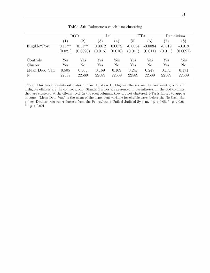
51

Table A6: Robustness checks: no clustering

ROR Jail FTA Recidivism(1) (2) (3) (4) (5) (6) (7) (8)

Eligible*Post 0.11∗∗∗ 0.11∗∗∗ 0.0072 0.0072 -0.0084 -0.0084 -0.019 -0.019(0.021) (0.0090) (0.016) (0.010) (0.011) (0.011) (0.011) (0.0097)

Controls Yes Yes Yes Yes Yes Yes Yes YesCluster Yes No Yes No Yes No Yes NoMean Dep. Var. 0.505 0.505 0.169 0.169 0.247 0.247 0.171 0.171N 22589 22589 22589 22589 22589 22589 22589 22589

Note: This table presents estimates of δ in Equation 1. Eligible offenses are the treatment group, andineligible offenses are the control group. Standard errors are presented in parentheses. In the odd columns,they are clustered at the offense level; in the even columns, they are not clustered. FTA is failure to appearin court. ‘Mean Dep. Var.’ is the mean of the dependent variable for eligible cases before the No-Cash-Bailpolicy. Data source: court dockets from the Pennsylvania Unified Judicial System. ∗ p < 0.05, ∗∗ p < 0.01,∗∗∗ p < 0.001.

52

Table A7: Difference-in-difference estimates of the effect of No-Cash-Bail policy on jail: differentlengths of jail time

Spent at least x nights in jail, with x equal to...1 2 3 4 5 6 7

Eligible*Post 02/21 0.0049 0.0070 0.0074 0.013 0.014 0.015 0.013(0.017) (0.017) (0.016) (0.015) (0.016) (0.016) (0.016)

Controls Yes Yes Yes Yes Yes Yes YesMean Dep. Var. 0.190 0.175 0.169 0.164 0.159 0.157 0.155N 22589 22589 22589 22589 22589 22589 22589

Note: This table presents estimates of δ in Equation 1. Eligible offenses are the treatment group, andineligible offenses are the control group. The outcome in each column is being detained pretrial for at least xnights after the bail hearing – Column 1 is at least 1 night, Column 2 is at least 2 nights, and so on. Controlsare for offense statute and class, age, gender, day of week, shift, presence and number of past offenses andpast FTAs, and initial bail commissioner. “Mean Dep. Var.” is the mean of the dependent variable foreligible cases before the No-Cash-Bail policy. Data source: court dockets from the Pennsylvania UnifiedJudicial System. ∗ p < 0.05, ∗∗ p < 0.01, ∗∗∗ p < 0.001. Standard errors, clustered at the offense level, arein parentheses.

53

Table A8: Regression discontinuity in time estimates of the No-Cash-Bail policy, for eligibleoffenses

(1) (2) (3) (4)ROR Jail (3+ nights) FTA Recidivism

Panel A: Full samplePost 02/21 0.104∗∗∗ -0.0356 0.0102 0.0394

(0.0282) (0.0204) (0.0268) (0.0227)Mean Dep. Var. 0.531 0.154 0.255 0.160Effective RD observations 3475 4437 4730 4633Bandwidth for estimation 41 52 57 56Bandwidth for bias 61 78 86 84Panel B: Cash BailPost 02/21 0.152∗∗ -0.0428 -0.0327 0.0239

(0.0494) (0.0339) (0.0365) (0.0271)Pre-reform mean 0.349 0.239 0.202 0.141Effective RD observations 1810 2678 2375 3150Bandwidth for estimation 38 58 50 68Bandwidth for bias 57 87 82 103

Note: This table presents regression discontinuity in time estimates of the effect of the No-Cash-Bail policy,for eligible offenses, following Calonico et al. (2014). Panel A presents results for the full sample. In PanelB, we subset eligible offenses to only include offenses that are most likely to have had cash bail (and notpretrial supervision) before the No-Cash-Bail reform, as defined in Table 5. ‘Mean Dep. Var.’ is the meanof the dependent variable for eligible cases before the No-Cash-Bail policy. Data source: court dockets fromthe Pennsylvania Unified Judicial System. ∗ p < 0.05, ∗∗ p < 0.01, ∗∗∗ p < 0.001.

54

Table A9: Robustness for difference-in-difference estimates of the effect of No-Cash-Bail policyon FTA and recidivism: different time windows

FTA within... Recidivism within...

1 month 3 months 10 months 1 month 3 months 10 months(1) (2) (3) (4) (5) (6)

Eligible*Post 02/21 0.0057 0.0029 -0.0041 -0.0026 -0.0081 -0.025∗

(0.0056) (0.0064) (0.010) (0.0049) (0.0081) (0.0093)

Controls Yes Yes Yes Yes Yes YesMean Dep. Var. 0.035 0.085 0.157 0.046 0.108 0.235N 22589 22589 20524 22589 22589 20524

Note: This table presents estimates of δ in Equation 1. Eligible offenses are the treatment group, andineligible offenses are the control group. The outcome in Columns 1-3 is FTA and in Columns 4-6 isrecidivism. They are defined as having missed one’s court date or failed to appear in court within 1 month(Columns 1 and 4), 3 months (Columns 2 and 5) or 10 months (Columns 3 and 6) within one’s initial courthearing. In Columns 3 and 6, we limit our sample to defendants for whom we observe outcomes for at least10 months after their initial court hearing. Controls are for offense statute and class, age, gender, day ofweek, shift, presence and number of past offenses and past FTAs, and initial bail commissioner. “MeanDep. Var.” is the mean of the dependent variable for eligible cases before the No-Cash-Bail policy. Datasource: court dockets from the Pennsylvania Unified Judicial System. ∗ p < 0.05, ∗∗ p < 0.01, ∗∗∗ p < 0.001.Standard errors, clustered at the offense level, are in parentheses.

55

Table A10: Testing balance in judge case characteristics

(1) (2) (3) (4) (5) (6)Felony Black Age Male Past FTA Past charges

Judge 1 0.0014 -0.023 -0.34 -0.0046 -0.0034 0.0083(0.0042) (0.012) (0.31) (0.013) (0.012) (0.013)

Judge 2 0.0075 0.0014 0.083 -0.0061 -0.0055 0.0032(0.0067) (0.011) (0.27) (0.0081) (0.0076) (0.011)

Judge 3 0.0042 -0.0022 -0.033 0.014 0.019∗ 0.014(0.0033) (0.0074) (0.26) (0.010) (0.0089) (0.010)

Judge 4 -0.0015 -0.0087 -0.21 -0.0040 -0.00100 0.012(0.0012) (0.011) (0.33) (0.0098) (0.0089) (0.0079)

Judge 5 0.0070 -0.0041 -0.18 0.0052 -0.0048 -0.00059(0.0049) (0.0088) (0.29) (0.0068) (0.0099) (0.0093)

Mean Dep. Var. 0.532 0.559 34.061 0.834 0.160 0.558N 21527 21527 21527 21527 21527 21527

Note: This table tests whether cases are quasi-randomly assigned to bail magistrates. To do so, we regressobservable case characteristics on dummies for bail magistrates, while controlling for day of the week, shift,quarter in the year, and offense. We drop cases that are not examined by judges who see at least 100 casesa year. “Mean Dep. Var.” is the mean of the dependent variable for eligible cases before the No-Cash-Bailpolicy. Data source: court dockets from the Pennsylvania Unified Judicial System. ∗ p < 0.05, ∗∗ p < 0.01,∗∗∗ p < 0.001. Standard errors, clustered at the offense level, are in parentheses.

56

Table A11: Difference-in-difference estimates of the effect of No-Cash-Bail policy on ROR, jail,FTA and Recidivism, keeping only felony cases

ROR Jail FTA Recidivism(1) (2) (3) (4)

Eligible*Post 02/21 0.17∗∗∗ -0.020 -0.010 -0.017(0.019) (0.020) (0.0086) (0.0090)

Controls Yes Yes Yes YesMean Dep. Var. 0.172 0.322 0.182 0.184N 12038 12038 12038 12038

Note: This table presents estimates of δ in Equation 1, keeping only felony cases. Eligible offenses are thetreatment group, and ineligible offenses are the control group. ROR (released on own recognizance) meansthat a defendant is released with no monetary or supervisory conditions. Pretrial detention is defined asspending at least 3 nights in jail immediately after their initial bail hearing. FTA means failure to appearin court. Recidivism (new criminal charges) is measured within 6 months after one’s initial court hearing.Controls are for offense statute and class, age, gender, day of week, shift, presence and number of pastoffenses and past FTAs, and initial bail commissioner. “Mean Dep. Var.” is the mean of the dependentvariable for eligible cases before the No-Cash-Bail policy. Data source: court dockets from the PennsylvaniaUnified Judicial System. ∗ p < 0.05, ∗∗ p < 0.01, ∗∗∗ p < 0.001. Standard errors, clustered at the offenselevel, are in parentheses.

57

Table A12: Comparing the characteristics of beneficiaries and of potential beneficiaries of theNo-Cash-Bail reform for cases other than PWID

Potential Ratio:Beneficiaries beneficiaries beneficiaries /(compliers) (compliers + potential

never-ROR) beneficiaries(1) (2) (3)

Black 0.11 0.43 0.26(0.71)

Hispanic 0.35 0.22 1.62(1.61)

White 0.50 0.34 1.49(0.49)

Percent below poverty 0.23 0.24 0.95(0.19)

Predicted recidivism 0.14 0.16 0.86(0.14)

Predicted FTA 0.28 0.27 1.06(0.10)

Note: This table presents the average characteristics of compliers, who are the beneficiaries of the No-Cash-Bail policy, to that of all potential beneficiaries of the No-Cash-Bail policy, which to say compliers ofnever-ROR. Calculations follow the methodology outlined in appendix A. We drop PWID (possession withintent to deliver) cases, whose classification into “eligible” and “ineligible” cases may be more ambiguous,since it depends on prior drug cases whose characteristics we do not fully observe in our data. Note that ourmain results are unchanged when we drop PWID cases (Table A11) In Column 3, we report standard errors(in parentheses) based on 1000 bootstrap replications.

58

Table A13: Difference-in-difference estimates of the effect of No-Cash-Bail policy on ROR, jail,FTA and Recidivism, dropping PWID cases

ROR Jail FTA Recidivism(1) (2) (3) (4)

Eligible*Post 02/21 0.099∗∗∗ 0.013 -0.014 -0.017(0.021) (0.016) (0.011) (0.015)

Controls Yes Yes Yes YesMean Dep. Var. 0.684 0.084 0.194 0.156N 17952 17952 17952 17952

Note: This table presents estimates of δ in Equation 1, dropping PWID (possession with intent to deliver)cases. Eligible offenses are the treatment group, and ineligible offenses are the control group. ROR (releasedon own recognizance) means that a defendant is released with no monetary or supervisory conditions. Pretrialdetention is defined as spending at least 3 nights in jail immediately after their initial bail hearing. FTAmeans failure to appear in court. Recidivism (new criminal charges) is measured within 6 months after one’sinitial court hearing. Controls are for offense statute and class, age, gender, day of week, shift, presence andnumber of past offenses and past FTAs, and initial bail commissioner. “Mean Dep. Var.” is the mean of thedependent variable for eligible cases before the No-Cash-Bail policy. Data source: court dockets from thePennsylvania Unified Judicial System. ∗ p < 0.05, ∗∗ p < 0.01, ∗∗∗ p < 0.001. Standard errors, clustered atthe offense level, are in parentheses.