bajd comp - eckner
TRANSCRIPT

Computational Techniques for basic Affine
Models of Portfolio Credit Risk
Andreas Eckner∗
First version: August 2007Current version: August 2009
Forthcoming in Journal of Computational Finance
Abstract
This paper presents computational techniques that make a certain class of fullydynamic intensity-based models for portfolio credit risk, along the lines of Duffieand Garleanu (2001) and Mortensen (2006), just as computationally tractable asthe Gaussian copula model. For this model, we improve the fit to tranche spreadsby a factor of around three, by allowing for a more flexible correlation structure,and by accounting for market frictions due to bid-offer spreads. The resultingmodel can be used to hedge a wide range of risks in the credit market, such as therisk of changes in correlations, volatilities, or idiosyncratic default risk.
Keywords: credit risk, correlated default, structured credit derivatives, affinejump diffusion, intensity-based model, CDO pricing
∗Department of Statistics, Stanford University. Comments are welcome at [email protected] source code of the implementation is available at http://www.eckner.com/research.html. Iwould like to thank Xiaowei Ding, Peter Feldhutter, Kay Giesecke, Tze Leung Lai, Allan Mortensenand George Papanicolaou for helpful comments and remarks, and especially Darrell Duffie for frequentdiscussions. I am grateful to Citi, Markit and Morgan Stanley for providing historical credit index andtranche spreads, and Markit for providing historical CDS spread data.

1 Introduction
We present computational techniques that make a fully dynamic, doubly stochastic,intensity-based model1 for the joint behavior of corporate default times, along the linesof Duffie and Garleanu (2001) and Mortensen (2006), just as tractable as the staticGaussian copula model (Li (2000)). Both model implementations have the recursivecalculation of the conditional (on the common factor) portfolio loss distribution, using analgorithm due to Andersen, Sidenius, and Basu (2003), as the computational bottleneck.2
In our implementation of this intensity-based model, the “ASB”-algorithm accounts for65% of the total computing time when pricing credit tranches. A modified version ofthe algorithm that avoids calculating the probability of extremely unlikely events, stillaccounts for 38% of the total computing time. Credit tranches can be priced in lessthan one second on a single-processor workstation,3 while calibration of the model for asingle day takes only a few minutes, given the fitted parameters from the previous day.
A second emphasis of this paper is to improve upon the model fit in Mortensen (2006)by a factor of around three, by allowing for a more flexible correlation structure, andby accounting for market frictions due to bid-offer spreads. We also show that a richclass of recovery rate scenarios can be incorporated into the model in a computationallytractable manner. The resulting model can be used to hedge a wide range of risks in thecredit market, such as the risk of changes in spread volatilities, or idiosyncratic defaultrisk - effects that cannot be considered in the inherently static copula model.
A tractable dynamic model for portfolio credit risk should be of interest to a varietyof researchers and practitioners. Although the Gaussian copula model is an industrystandard, its theoretical foundations such as implied default and credit spread dynamicsare often quite unrealistic. Tranches of CDOs usually cannot be priced consistently usinga single correlation parameter, which has given rise to the base correlation framework,even though it does not guarantee arbitrage-free prices. For these reasons, variousauthors have considered extensions such as the Clayton, Student-t, double-t, or Marshall-Olkin copulas. See Burtschell, Gregory, and Laurent (2005) for a comparative analysis.Nevertheless, current models of this type cannot capture the dynamics of credit spreadsand are therefore unsuitable analyzing certain risk dimensions (such as mark-to-marketrisk and collateral agreements4) and for pricing securities whose payout depends on credit
1Standard references on intensity-based models, sometimes called reduced-form models, include Jar-row and Turnbull (1995), Lando (1998), and Duffie and Singleton (1999).
2Jackson, Kreinin, and Ma (2007) found this algorithm to be preferable to Fourier based convolutionmethods, as long as the portfolio contains only a couple of hundred issuers. From talking with prac-titioners we learned that the recursive Andersen-Sidenius-Basu step currently is indeed the preferredmethod for the one-factor Gaussian copula model.
3This computing time applies to a hybrid C/Matlab model implementation on a computer with1.86Ghz Intel R© Celeron R© processor with 1GB of RAM. A pure C implementation would likely be twoto three times faster.
4Incorrect assessment of the later type of risk triggered a liquidity crisis at American In-
2

spread dynamics (such as options on CDS indices). On the other hand, these featurescan be incorporated in a natural way into an intensity-based framework of credit risk.Due to the rapid growth of the market for credit derivatives over the past decade,intensity-based models of credit risk are currently an active area of research. See forexample Duffie and Garleanu (2001), Giesecke and Goldberg (2005), Errais, Giesecke,and Goldberg (2006), Joshi and Stacey (2006), Mortensen (2006), Papageorgiou andSircar (2008), and Longstaff and Rajan (2008).
In our analysis we rely heavily on the doubly stochastic assumption for default inten-sities, so that correlation of default intensities is the only mechanism by which correlationof default times can arise. While computationally convenient, it is important to keep inmind that this framework rules out some important other channels of default correlation,such as unobservable risk-factors (frailty) and contagion. See, for example, Das, Duffie,Kapadia, and Saita (2007), Duffie, Eckner, Horel, and Saita (2009), and Ding, Giesecke,and Tomecek (2008). However, for alternative bottom-up specifications that relax thedoubly-stochastic assumption, computational tractability may an issue. As opposed toa bottom up model as ours, where the primitives are the intensity processes of the indi-vidual firms, top-down models directly specify the portfolio loss process in terms of anintensity process. Such models more easily allow the relaxation of the doubly stochasticassumption while retaining computational tractability. However, additional non-trivialsteps are required to calibrate the single names in the portfolio.
The rest of the paper is organized as follows. The remainder of this Section describessome of the most common credit derivatives and the data sources used for our analysis.Section 2 introduces the model for risk-neutral default times, while Section 3 presentsvarious computational techniques. Section 4 present the pricing of credit derivatives inthis setup and the model calibration algorithm. Section 5 examines the model fit at afixed point in time and discusses hedging of credit tranches. Section 6 concludes andsuggests possible model extensions.
1.1 Credit Derivative Contracts
A credit derivative is a contract whose payoff is linked to the creditworthiness of one ormore obligations. This section summarizes the features of the three most common typesfor corporate credit risk.
Credit Default Swaps. By far the most common credit derivative is the creditdefault swap (CDS). It is an agreement between a protection buyer and a protectionseller, whereby the buyer pays a periodic fee in return for a contingent payment by theseller upon a credit event, such as bankruptcy or “failure to pay”, of a reference entity.
ternational Group in September 2008 with subsequent rescue by the Federal Reserve. Seehttp://www.federalreserve.gov/newsevents/press/other/20080916a.htm for details.
3

The contingent payment usually replicates the loss incurred by a creditor of the referenceentity in the event of its default. See, for example, Duffie (1999).
Credit Indices. A credit index contract allows an investor to either buy or sellprotection on a basket of reference entities, and therefore closely resembles a portfo-lio of CDS contracts. For example, the CDX.NA.IG (for CDS index, North America,Investment Grade) contract provides equally-weighted default protection on 125 NorthAmerican investment-grade rated issuers. For a more detailed description see the ’CreditDerivatives Handbook’ (2006) by Merrill Lynch.
Credit Tranches. A credit tranche allows an investor to gain a specified exposureto the credit risk of the underlying portfolio, while in return receiving periodic couponpayments. Losses due to credit events in the underlying portfolio are allocated first tothe lowest tranche, known as the equity tranche, and then to successively prioritizedtranches. The risk of a tranche is determined by the attachment point of the tranche,which defines the point at which losses in the underlying portfolio begin to reduce thetranche notional, and the detachment point, which defines the point at which losses inthe underlying portfolio reduce the tranche notional to zero. The buyer of protectionmakes coupon payments on the notional amount of the remaining size of the tranche,which is the initial tranche size less losses due to defaults. This structure is illustratedin Table 1 for the CDX.NA.IG index.
Tranche Attachment Point Detachment Point Quote ConventionEquity 0% 3% 500 bps running + upfrontJunior Mezzanine 3% 7% all runningMezzanine 7% 10% all runningSenior Mezzanine 10% 15% all runningSenior 15% 30% all runningSuper Senior 30% 100% all running
Table 1: Tranche structure of the CDX.NA.IG index, which has 125 equally weighted North-American
investment-grade issuers in the underlying portfolio.
The coupon payments for these three contracts are typically made quarterly, on the20th of March, June, September, and December, unless this date is a holiday, in whichcase the payment is made on the next business day. If a contract is entered in betweentwo such dates, the buyer of protection receives from the seller of protection the accruedpremium since the last coupon date.
4

1.2 Data Sources
Citi and Morgan Stanley provided 5, 7, and 10-year CDX.NA.IG index and tranche bid-and ask-spreads. Markit provided 5, 7, and 10-year CDX.NA.IG tranche mid-marketspreads, and 1, 5, 7, and 10-year CDS mid-market spreads for the CDX.NA.IG members.
We used 3-month, 6-month, 9-month, 1-year, 2-year, ..., 10-year US LIBOR swaprates to estimate the discount function Bt (T ) at each point in time t. Specifically, forthese standard maturities we used swap rates from the Bloomberg system, while fornon-standard maturities we used cubic-spline interpolation of implied forward rates todetermine the spot rate. Swap rates are widely regarded as the best measure of fundingcosts for banks - the biggest participant in the market for synthetic credit derivatives -over various time horizons.
2 Model Setup
This section describes a model for the joint distribution of various obligor default timesunder a risk-neutral probability measure. To this end, we fix a filtered probability space(Ω,F , (Ft) ,P) satisfying the usual conditions.5 Up to purely technical conditions,6 theabsence of arbitrage implies the existence of an equivalent martingale measure Q, suchthat the price at time t of a security paying an amount Z at a stopping time τ > t isgiven by
Vt = EQt
(e−
∫ τ
trsdsZ
),
where r is the short-term interest rate and EQt denotes expectation under Q, conditional
on all available information up to time t.Under the equivalent martingale measure Q, for each individual firm i, a default time
τ i is modeled using Cox processes, also known as doubly stochastic Poisson processes.See for example Lando (1998) and Duffie and Singleton (2003). Specifically, the defaultintensity of obligor i is a non-negative real-valued progressively measurable stochasticprocess, which will be defined below. Conditional on the intensity path λit : t ≥ 0, thedefault time τ i is taken to be the first jump time of an inhomogeneous Poisson processwith intensity λi. In particular, the default times of any set of firms are conditionallyindependent given the intensity paths, so that correlation of default intensities is theonly mechanism by which correlation of default times can arise.
For t > s, risk-neutral survival probabilities can be calculated via
Q (τ i > t | Fs) = EQs (Q (τ i > t | λit : t ≥ 0 ∪ Fs)) = 1τ i>sE
Qs
(e−
∫ t
sλiudu
), (1)
5For a precise mathematical definition not offered here, see Karatzas and Shreve (2004), and Protter(2005).
6See Harrison and Kreps (1979), Harrison and Pliska (1981), and Delbaen and Schachermayer (1999).
5

where the expectation is taken over the distribution of possible intensity paths. Thelarge and flexible class of affine processes allows one to calculate (1) either explicitly ornumerically quite efficiently. See Duffie, Pan, and Singleton (2000).
Due to their computational tractability, we use basic Affine Jump Diffusions (AJD)as the building block for the default intensity model. Specifically, we call a stochasticprocess Z a basic AJD under Q if
dZt = κ(θ − Zt) dt+ σ√Zt dBt + dJt, Z0 ≥ 0, (2)
where under Q, (Bt)t≥0 is a standard Brownian motion, and (Jt)t≥0 is an independentcompound Poisson process with constant jump intensity l and exponentially distributedjumps with mean µ. For the process to be well defined, we require that κθ ≥ 0 andµ ≥ 0. Note that (2) is a special case of more general affine processes, see for exampleDuffie, Filipovic, and Schachermayer (2003).
Basic AJDs are especially attractive for modeling default times, since both the mo-ment generating function
m (q) = EQ(eq
∫ t
0Zsds), q ∈ R, (3)
and the characteristic function
ϕ (u) = EQ(eiu
∫ t
0Zsds), u ∈ R, (4)
are known in closed-from, see Appendix A for details. In particular, if Z is the defaultintensity of a certain obligor, setting q = −1 in (3) allows one to explicitly calculate theobligor’s survival probability (1). In addition, the characteristic function (4) allows oneto calculate the density of an integrated basic AJD
Zt ≡∫ t
0
Zsds
by Fourier inversion, as discussed in Section 3.2 below.
2.1 Risk-Neutral Default Intensities
We now make precise the multivariate model of default times. The risk-neutral defaultintensity of obligor i is
λit = Xit + aiYt, (5)
with idiosyncratic component Xi and systematic component Y . As in Duffie andGarleanu (2001) and Mortensen (2006), under Q, X1, . . . , Xm and Y are independentbasic AJDs, with
dXit = κi(θi −Xit)dt+ σi
√Xit dB
(i)t + dJ
(i)t (6)
dYt = κY (θY − Yt)dt+ σY
√Yt dB
(Y )t + dJ
(Y )t . (7)
6

Here, J (Y ) and J (i) have jump intensities lY and li, and jump size means µY and µi, re-spectively. Hence, jumps can either be firm-specific or market-wide. Duffie and Garleanu(2001) and Mortensen (2006) found the latter type of jumps in default intensities to becrucial for explaining the spreads of senior CDO tranches, which are heavily exposedto tail risk events. Schneider, Sogner, and Veza (2009) examined the time series of 282credit default swap spreads and found evidence for mainly positive jumps in defaultintensities.
2.1.1 Parameter Restrictions
This section discusses restrictions on the parameters in (6) and (7) that (i) make themodel identifiable and (ii) reduce, for parsimony, the number of free parameters. Wealso point out the differences between our model setup and those of Duffie and Garleanu(2001) and Mortensen (2006). For a discussion about the suitability of such restrictionssee Feldhutter (2007).
Model Identifiability. The restriction
1
m
m∑
i=1
ai = 1
is imposed to ensure identifiability of the model.7
Parsimony. Our model specification is relatively general with 5m+5 default intensityparameters and m + 1 initial factor values. Since we are especially interested in theeconomic interpretation of the parameters, we favor a parsimonious model which isnevertheless flexible enough to closely fit tranches spreads. First, we take the commonfactor loading ai of each obligor i to be equal to the obligor’s 5-year CDS spread dividedby the average 5-year CDS spread of the current credit index members, that is
ai =ccdsi,t,M
Avgi(ccdsi,t,M
) , (8)
7If all factor loadings ai are replaced by cai for some positive constant c, then replacing the param-eters (Y0, κY , θY , σY , lY , µY ) with (Y0/c, κY , θY /c, σY /
√c, lY , µY /c) leaves the dynamics of aiY (and
therefore also the joint dynamics of λi) unchanged.
7

where ccdsi,t,M denotes the 5-year CDS spread at time t for the ith reference entity. More-over, we impose the parameter constraints
κi = κY ≡ κ, (9)
σi =√aiσY ≡ √
aiσ, (10)
µi = aiµY ≡ aiµ, (11)
ω1 =lY
li + lY, (12)
ω2 =aiθY
aiθY + θi, (13)
which reduces the number of free parameters to just seven. Feldhutter (2007) examines towhat extent (8)-(13) are empirically supported by CDS data for firms in the CDX.NA.IGindex, and finds these assumptions in general to be fairly reasonable.
The constraints (8)-(13) imply that λi is a basic AJD, which is not generally thecase for the sum of two basic AJDs, see Duffie and Garleanu (2001), Proposition 1.Specifically,
dλit = κ ((θi + aiθY )− λit) dt+√aiσ√λit dB
(i)t + dJ
(i)t ,
or in short-hand
λi = bAJD(λi,0, κ, θi + aiθY ,√aiσY , li + lY , µi) =
= bAJD(λi,0, κ, θi, σi, l, µi),
where θi = θi + aiθY and l = li + lY .It is easy to show that θY = ω2Avg(θi) ≡ ω2θAvg and that θi = aiθAvg for each i,
so that we can characterize the joint risk-neutral model of default times with the sevenparameters
Θ =κ, θAvg, σ, l, µ, ω1, ω2
,
and the m + 1 initial factor values. Even though the above constraints greatly reducethe number of free parameters, a model without these constraints would be just ascomputationally tractable, since the computational techniques described below do notmake use of (8)-(13).
Remark 1 The model setup in this section is slightly more general than that of Mortensen(2006), which in turn is a generalization of Duffie and Garleanu (2001), who examineda homogenous portfolio so that in particular all factor loadings ai are equal to one.Mortensen (2006) imposed
ω1 = ω2 =Y0
Y0 + Avg (Xi0),
so that the jump-correlation structure and mean-reversion levels are determined by theinitial values of the m+ 1 factors.
8

3 Computational Techniques
This section describes computational techniques for pricing credit derivatives in thebasic AJD framework of Section 2. Apart from Section 3.1 and 3.2, the techniques areapplicable to other credit derivative pricing models as well. The modified Andersen-Sidenius-Basu algorithm, for example, allows one to compute the conditional portfolioloss distribution for any factor model, no matter whether dynamic or static, wheredefault times are conditionally independent given the common factors. Similarly, themodel for stochastic and serially correlated recovery rates applies to any model whererecovery rates are independent of default times.
3.1 Survival Probabilities
In the affine two-factor model of Section 2.1,
Q (τ i > t | Fs) = 1τ i>sEQs
[e−
∫ t
sXi,udu
]EQ
s
[e−ai
∫ t
sYudu
]. (14)
The expectations on the right-hand side can be calculated explicitly by evaluating themoment generating function (3) at q = −1.
3.2 Common Factor Distribution
Mortensen (2006) derived a system of ODEs, whose solution yields the characteristicfunction (4). Appendix A.2 shows that this characteristic function is actually known inclosed-form. The distribution of the integrated common factor
Ys,t ≡∫ t
s
Yu du
can therefore be efficiently calculated by Fourier inversion, which was done by carryingout the following steps:
1. Evaluate the characteristic function of Ys,t on an unequally spaced grid of length1024 with mesh size smallest for grid points close to 0, for example by using anequally-spaced grid on a logarithmic scale.
2. Fit a complex-valued cubic spline to the output from step 1, and evaluate the cubicspline on an equally spaced grid with 218 points.
3. Apply the Fast Fourier Transform (FFT) to the output from step 2 to obtain the
density of Ys,t evaluated on an equally-spaced grid.
See Cerny (2004) for a general introduction to the FFT, and Carr and Madan (1999),Section 4 for details regarding the spacing of input and output points.
9

3.3 Conditional Distribution of Defaults
By construction, conditional on the integrated common factor Ys,t, defaults in the timeinterval (s, t] occur independently. At time s, the conditional distribution Ps,t of thenumber of defaults in the portfolio up to time t can therefore be computed using therecursive algorithm of Andersen, Sidenius, and Basu (2003) (ASB in the following).Specifically, let
qi(Ys,t) = Qs
(s < τ i ≤ t | Ys,t
)= 1τ i>s
(1−EQ
s
[e−
∫ t
sXi,udu
]e−aiYs,t
)(15)
denote the conditional default probability of the ith issuer, and P(n)s,t (k | Ys,t) denote the
conditional probability that k of the first n credits in the portfolio default between timess and t. The following recursive updating scheme allows one to calculate the distributionof the number of defaults in the portfolio conditional on Ys,t:
P(0)s,t (k | Ys,t) = 1k=0, (16)
P(n+1)s,t (k | Ys,t) = qn+1(Ys,t)P
(n)s,t (k − 1 | Ys,t) + (1− qn+1(Ys,t))P
(n)s,t (k | Ys,t),
for 0 ≤ k ≤ n and 0 ≤ n < m.
Modified ASB-Algorithm The algorithm (16) can be modified so as to considerablyincrease its speed. Specifically, we restrict the ASB-algorithm to values of k, such thatPs,t(k | Ys,t) > ε for some small number ε, for example 10−10. Otherwise, the algorithmspends a large amount of time computing the probability of events that are extremelyunlikely to occur, and therefore have a negligible impact on credit tranche spreads.8
To this end, for a given value of the integrated common factor Ys,t, let
d(Ys,t) = d(Ys,t, s, t) =
m∑
i=1
qi(Ys,t)
denote the conditional (on the integrated common factor) expected number of defaultsin the portfolio during the time interval (s, t]. Under certain conditions, the Poisson
approximation (see for example Durrett (2005), Theorem 6.1) implies that Ps,t(k | Ys,t)is close to a Poisson distribution with parameter d(Ys,t) so that
Ps,t(k | Ys,t) ≈d(Ys,t)
ke−d(Ys,t)k
k!.
8A trivial but significant speed-up can also be achieved by replacing exp(−aiYs,t) in (15) with its
Taylor series approximation for small values of aiYs,t.
10

Hence, we restrict the ASB-algorithm in (16) to values k ≤ K (ε), where
K (ε) = min
K :
d(Ys,t)le−d(Ys,t)l
l!< ε for l ≥ K
, (17)
which leads to significant computational savings, since the conditional expected numberof defaults d(Ys,t) is usually quite small, so that K (ε) is small too.9
3.4 Unconditional Distribution of Defaults
Recall that the output of the Fourier inversion steps is the density of Ys,t evaluated onan equally spaced grid (yi = i∆y : 0 ≤ i < N), where ∆y is the spacing of the grid, andN the number of points used in the FFT. The unconditional probability Ps,t (k) of k
defaults in the portfolio can therefore be obtained by integration of Ps,t(k | Ys,t) over thedistribution of Ys,t:
Ps,t (k) =
∫Ps,t(k | Ys,t) dQ(Ys,t) ≈ (18)
≈N∑
i=1
Ps,t(k | yi)fYs,t(yi)∆y ≡ Ps,t (k)
Since the integrand in (18) is quite costly to evaluate, this computation is extremelytime-consuming for large values of N . Nevertheless, this calculation can be done quiteefficiently by exploiting the smoothness of the probability Ps,t(k | Ys,t) in Ys,t.
To this end, let FYs,tdenote the cumulative distribution function of Ys,t. For some
number N2 ≪ N , calculate the quantiles
γi = F−1
Ys,t
(i
N2
), 0 ≤ i ≤ N2.
With this notation, (18) can be written as a sum of integrals
Ps,t (k) =
N2∑
i=1
∫ γi
γi−1
Ps,t(k | Yt)dQs(Ys,t). (19)
The integrals in (19) can be evaluated, for example, by Gauss-Legendre integration, and
we denote the resulting approximation of the distribution Ps,t by Ps,t.10
9We found using a boundary value of K = 8+ d(Ys,t) + 8
√d(Ys,t) to work just as well, but faster to
calculate than (17). The functional form of this expression is motivated by that fact that the mean andstandard deviation of a Poisson random variable with parameter λ are equal to λ and
√λ, respectively.
10Alternatively, one could use an adaptive quadrature method. However, since the distribution of Ys,t
tends to be highly skewed with very narrow peak and since the integrand in (18) is costly to evaluate,we found it advantageous to aid the numerical quadrature procedure by breaking down the integrationrange into sub-intervals based on the quantiles of the distribution of Ys,t.
11

We found using N2 = 250 and Gauss-Legendre integration with five support pointsto be very fast and accurate for calculating the unconditional distribution Ps,t of thenumber of defaults. For the fitted models of Section 5.1, the approximation error fromthe numerical integration was found to satisfy
∥∥∥Ps,t − Ps,t
∥∥∥TV
=1
2
m∑
k=0
∣∣∣Ps,t (k)− Ps,t (k)∣∣∣ < 10−7
for a time horizon t − s equal to five years, where ‖·‖TV denotes the total variationnorm.11
3.5 Multiple Horizons
This sections discusses an interpolation method for efficiently calculating the uncondi-tional distribution of the number of defaults Ps,t for multiple time horizons t. Since theloss distribution Ps,t varies smoothly in t, it is only necessary to calculate this distribu-tion on a sparse grid of time horizons T = t0, t1, . . . , tl. As hinted by Mortensen(2006), interpolation techniques can then be used to evaluate Ps,t at non-grid points.
To this end, assume Ps,t is already known for t ∈ T and that we want to computePs,t for a time horizon t with t /∈ T . For each k with 0 ≤ k ≤ m, let wt (k) denote thecubic spline interpolation of the data
(tj, Ps,tj (k)
): 0 ≤ j ≤ l
evaluated at t. Then
Ps,t (k) =wt (k)∑mn=0wt (n)
, 0 ≤ k ≤ m, (20)
can serve as an estimate of the distribution Ps,t of the number of defaults in the timeinterval (s, t].
For the fitted model of Section 5.1, an analysis of the approximation error as afunction of the grid spacing in T showed that the approximation (20) is extremelyaccurate up to a yearly spacing. Even a coarse two-year spacing resulted in a relativepricing error of less than 0.2% for each single tranche. To summarize, interpolatingthe distribution of the number of defaults Ps,t over t can speed up the pricing of credittranches by a factor of at least four.
3.6 Recovery Rates and Portfolio Loss Distribution
A large portion of tranche pricing models in the literature, such as the Gaussian Copulamodel, implicitly assume deterministic recovery rates. However, a couple of empiricalfeatures of recovery rates should be considered:
11For the CDX tranches on this particular date, the approximation error resulted in a relative pricingerror of less than 0.05% for each single tranche.
12

1. Stochastic recovery rates: Moody’s (2000) reports a large cross-sectional dispersionof defaulted debt recovery for senior unsecured bonds (often taken as the referenceentities for credit default swaps) of US corporations between 1970 and 1998. The25th, 50th and 75th percentile of recovery rates were roughly 30%, 50% and 65%,respectively. For 1989 to 1995, Altman and Kishore (1996) found recoveries forsenior unsecured debt were on average 47% with a sample standard deviation of27%.
2. Correlation of recovery rates with macroeconomic conditions: Moody’s (2000), andAltman, Bray, Resti, and Sironi (2005) find that recovery rates behave counter-cyclical, that is, recovery rates tend to be low when corporate default rates arehigh, and vice versa. In particular, recovery rates are positively serially correlated.
The remainder of this section shows how to incorporate stochastic and serially cor-related recovery rates into the basic AJD framework of Section 2.1. To retain com-putational tractability, recovery rates are however still assumed to be independent ofmacroeconomic conditions, so that property one is fully, and property two partiallyincorporated into the model. To this end, let
Ls,t (x) = Qs
(1
m
m∑
i=1
(1− Ri) 1s<τ i≤t ≤ x
)(21)
denote the cumulative fractional portfolio loss distribution between times s and t, wherex ∈ [0, 1]. Here Ri denotes the recovery rate of the ith firm, whose probabilistic proper-ties will be defined shortly.
If, under Q, recovery rates and default times are independent, then (21) can bewritten as
Ls,t (x) =m∑
k=0
Ps,t (k)Gk (x) , (22)
where for each k, Gk is the cumulative portfolio loss distribution conditional on k de-faults, which does not depend on the time points s and t. Thus, one can incorporate arich class of recovery rate scenarios, not only into the basic AJD framework of Section2.1, but into any model of portfolio credit risk that allows for the decomposition (22).
Example 1 The case of deterministic recovery rates equal to 40%, a common industry
13

practice for senior unsecured corporate debt,12 corresponds to the choice
Gk (x) = 1 km(1−0.4)≤x.
Example 2 Stochastic recovery rates can be incorporated, for example, by fitting G1 tohistorical data and taking
Gk (x) = (G1 ∗Gk−1) (x)
for k ≥ 2, where ’∗’ denotes the convolution operator for random variables . Section 5.1examines the model fit for the particularly simple choice
G1 (x) =2
31x=0.45 +
1
31x=0.9, (23)
which matches the first two moments of historical recovery rates.
Appendix C discusses a choice for the conditional loss distributions Gk that corre-sponds to stochastic and serially correlated recovery rates.
4 Pricing and Model Calibration
This section discusses the pricing of various credit derivatives and the model calibrationto market prices.
4.1 Pricing
For the purpose of pricing credit risky securities, we adopt the widely used assumption:
Assumption 1 Under the risk-neutral probability measure Q,
(i) Default intensities and interest rates are independent.
(ii) Recovery rates are independent of default intensities.
12As elaborated by Duffie and Singleton (1997), and Duffie and Singleton (1999) it is in generaldifficult to separately identify risk-neutral recovery rates and default intensities. Even in cases in whichone has multi-horizon data available, as in Pan and Singleton (2008), recovery rate estimates seem to besensitive to the chosen model. Even though Pan and Singleton (2008) focus on sovereign CDS contracts,they show that this assumption is quite innocuous as long as the unknown true expected recovery rateis not close to 100%.
14

The first assumption has been found to be fairly innocuous, for example, Brigo andAlfonsi (2004) find no significant correlation between default intensities and interestrates, although Feldhutter and Lando (2004) and Driessen (2005) find a slightly positivecorrelation. However, in light of the 2007-2008 credit crunch, this conclusion mighthave to be revised. Nevertheless, for CDOs during this credit crisis, interest rate riskhas been dwarfed by credit spread and default risk. Regarding the second assumption,Altman, Bray, Resti, and Sironi (2005) and Moody’s (2000) find that recovery rates tendto behave counter-cyclical, at least under the physical probability measure.
The general procedure for pricing credit derivatives is setting the value of the fixedleg (the market value of the payments made by the buyer of protection) equal to thevalue of the protection leg (the market value of the payments made by the seller ofprotection) and to solve for the fair credit spread.
4.1.1 CDS and Credit Index Pricing
It is well known (see Appendix B.1 for details) that under Assumption 1 it is onlynecessary to calculate the conditional survival probabilities (14) for the set of futurecoupon payment dates tl : 1 ≤ l ≤ n, in order to price a CDS contract. Similarly,knowledge of these survival probabilities for all companies in a portfolio is sufficient forpricing the corresponding credit index contract. Hence, in the basic AJD framework ofSection 2.1, model-implied CDS and credit index spreads can be calculated explicitly.
4.1.2 Tranche Pricing
For a given point in time t, let
N trj,t =
(Aj − Aj
)−[max
(Ls,t −Aj , 0
)−max
(Ls,t − Aj, 0
)]
denote the remaining notional size of tranche j, where Aj and Aj denote the trancheattachment and detachment point, respectively. As shown in Appendix B.3, calculat-ing the market value of the fixed and protection leg of a tranche j requires calculat-ing the expected tranche size EQ
s (Ntrj,tl
) for the set of future coupon payments dates,tl : 1 ≤ l ≤ n. We therefore never need to calculate the portfolio loss distribution(22), but can directly compute the expected tranche size as
EQs (N
trj,tl
) = N
[(Aj −Aj)−
m∑
k=0
Ps,tl (k) Ij (k)
], (24)
where
Ij (k) =
∫ 1
Aj
min(x− Aj, Aj −Aj
)dGk (x) (25)
is the risk-neutral expected loss for tranche j conditional on k defaults. The integralsin (25) need to be computed only once, and can then be stored for later use.
15

4.2 Computing Times
In summary, in the basic AJD framework of Section 2.1, model-implied CDS, creditindex, and credit tranche spreads can be calculated explicitly, or at least quite efficiently,using various computational techniques. Table 2 lists the computing times for somecommonly used operations. In particular, it shows that the modified ASB step takes upabout 38% of the total computing time when pricing credit tranches, while the originalversion of the ASB algorithm would have accounted for more than 65%. The overallcomputational tractability of the basic AJD model is therefore on the same order ofmagnitude as that of the static Gaussian copula model, which, in its currently preferredimplementation, also relies on the recursive ASB step (16).
Task Environment % of TimeEvaluating the characteristic function (4) C 7.5%Cubic spline interpolation of characteristic function C & Matlab 24.1%FFT Matlab 16.5%Modified ASB-algorithm C 38.3%Other Matlab 13.5%
Table 2: Percentage of time spent on various operations when calculating tranche spreads in the
basic AJD framework of Section 2. This breakdown of computing times applies to a hybrid C/Matlab
model implementation on a computer with 1.86Ghz Intel R© Celeron R© processor with 1GB of RAM.
Computing times exclude internal Matlab overhead, which was less than 25%.
4.3 Market Frictions
When pricing credit derivatives one must account for various market frictions, as wellas for certain trading conventions in this market.
First, credit indices and credit tranches recognize only bankruptcy and “failure topay” as credit events, whereas CDS contracts usually also include certain forms of re-structuring. For the latter credit event type, the cheapest-to-deliver option for a buyerof protection via a CDS can potentially be quite valuable, as was the case for the Con-seco debt restructuring in 2000.13 For an extensive dataset of CDS quotes between 2000and 2005, Berndt, Jarrow, and Kang (2007) report a 2.35% median contribution of themodified-restructuring premium to total 5-year CDS spreads.
Second, index arbitrage traders are the medium by which the level of a CDS indexis kept in line with so-called intrinsics, which is the fair index level implied by indi-vidual CDS spreads. Whenever intrinsics differ from the current index level, traderscan profitably buy protection via the index and sell protection via the underlying CDS
13SEC filing available at www.secinfo.com/dRx61.5Yk.1.htm
16

contracts, or vice versa. Although there are currently plans underway to automate andcentralize CDS trading, the data used in this analysis covers a time period during whichtrading a large portfolio credit default swaps was a labor-intensive process, normallytaking several hours to complete. An index arbitrage trader therefore faces significantexecution risk, especially during periods of time when the index-CDS basis is volatile.Because of this risk and the cost of paying the bid-offer spread when trading individualcredit default swaps, index arbitrage traders only become active when the index leveldiffers by at least a couple of basis points from the intrinsics. As a consequence, theindex-CDS basis and index-tranche basis are generally non-zero and time-varying.
To account for these effects, we relate the fixed legs V cds,Fixedi of the underlying CDS
contracts to the fixed leg V idx,Fixed of a credit index at time t via
m∑
i=1
V cds,Fixedi (t) = V idx,Fixed (t)
(1 + bcds,idx (t)
), (26)
where bcds,idx (t) is the multiplicative index-CDS basis. Similarly, we relate the tranchefixed legs to the index fixed leg via
J∑
j=1
V tr,Fixedj (t) = V idx,Fixed (t)
(1 + btr,idx (t)
), (27)
where btr,idx (t) is the multiplicative index-tranche basis.14 From (26) and (27) it followsthat the index-CDS and index-tranche basis, when measured in basis points, are givenby cidxt,Mb
cds,idx and cidxt,Mbcds,idx, respectively, where cidxt is the index coupon at time t.
4.4 Model Calibration
This section links model-implied and mid-market CDS, credit index, and credit tranchespreads. To this end, let ctrj,t,M (S) for S ∈ MI,MK denote the spread at time t of thejth tranche with maturity M (usually 5, 7 or 10 years) as implied by the model (MI),or as reported by Markit (MK). Similarly, let ccdsi,t,M (MK) denote the spread at time tof the ith CDS with maturity M , as reported by Markit. Finally, let cidxt,M (C) be theM−year index spread at time t as reported by Citi.
We use a fitting criterion of the form15
C (Θ) = ωtrRMSEtr (Θ,M)2 + ωcdsRMSEcds (Θ,M)2 + (28)
ωidxRMSEidx (Θ,M)2 ,
14The summation on the right-hand side of (27) includes the super senior (30-100%) tranche.15Such a fitting criterion arises naturally in a likelihood framework with noisy observations. See
Eckner (2007) for details.
17

with weights ωtr, ωcds and ωidx. Here, RMSEtrt is the relative root mean square tranche
pricing error at time t, defined by
RMSEtrt (Θ,M) =
√√√√ 1
J
1
|M|
J∑
j=1
∑
M∈M
(ctrj,t,M (MI)− ctrj,t,M (MK)
ctrj,t,M (MK)
)2
, (29)
RMSEcdst is the relative root mean square CDS pricing error at time t,
RMSEcdst (Θ,M) =
√√√√ 1
m
1
|M|
m∑
i=1
∑
M∈M
(ccdsi,t,M (MI)− ccdsi,t,M (MK)
ccdsi,t,M (MK)
)2
, (30)
and RMSEidxt is the relative root mean square credit index pricing error at time t,
RMSEidxt (Θ,M) =
√√√√ 1
|M|∑
M∈M
(cidxt,M (MI)− cidxt,M (C)
cidxt,M (C)
)2
. (31)
The following algorithm was used for minimizing (28), that is, for fitting the basicAJD model of Section 2.1 to market-observed CDS, credit index, and credit tranchespreads:
Algorithm 1
1. For fixed parameter vector Θ and initial systematic intensity Y0, individual CDSspreads are calibrated by varying the initial intensities λi0 for 1 ≤ i ≤ m subject tothe constraint λi0 ≥ aiY0, and minimizing the fitting criterion (30).
2. Set bcds,idx = btr,idx = 0 and determine the model implied CDS, index and tranchespreads. Solve for the index-CDS basis bcds,idx in (26), and for the index-tranchebasis btr,idx in (27). At each revision of bcds,idx, Step 1 is repeated.
3. Vary the parameter vector Θ and the initial systematic intensity Y0 to minimizethe criterion function (28). At each revision of Θ or Y0, Step 1 and 2 are repeated.
Step 3 was implemented by fitting each parameter separately and iterating over theset of parameters. Convergence typically occurred after 20 to 30 iterations.
5 Results
This section examines the fit of the model to tranche spreads of the CDX.NA.IG index ata fixed point in time, namely December 5, 2005, to facilitate comparison with Mortensen(2006). Since the emphasis of this paper are computational techniques, we focus onlyon a single point in time. See Eckner (2007) for a time series analysis of tranche spreadsand the evolution of calibrated parameters and fitting errors over time.
18

5.1 5 year Maturity
We start by examining the simultaneous model fit to 5-year CDS, credit index, andcredit tranche spreads, using
C(Θ) = RMSEtrt (Θ, 5) + 5× RMSEcds
t (Θ, 5) + 5× RMSEidxt (Θ, 5)
as the fitting criterion.16 Table 3 shows the model fit of Mortensen (2006) and of themodel from Section 2 with deterministic recovery rates (see Example 1). For brevity wedenote this model as bAJD. Models denoted by bAJD+ and bAJD++ additionally incor-porate stochastic recovery rates (see Example 2), and stochastic and serially correlatedrecovery rates (see Appendix C), respectively.
Tranche Bloomberg Mort Markit Citi MS bAJD bAJD+ bAJD++
0% - 3% 41.1% 43.2% 40.7% 40.8% 41.1% 40.2% 39.8% 40.2%3% - 7% 117.5 125.9 111.9 112.5 113.5 121.7 128.6 122.17% - 10% 32.9 30.6 31.3 31.3 31.0 28.5 28.0 30.010% - 15% 15.8 21.3 13.5 13.5 14.5 14.6 14.8 14.415% - 30% 7.0 8.8 7.4 7.5 7.3 7.2 7.2 7.2
RMSEtr(Θ, 5) - 0.200 - - - 0.069 0.093 0.062
RMSEcds(Θ, 5) - - - - - 0.000 0.000 0.000
RMSEidx(Θ, 5) - - - - - 0.000 0.000 0.000
Table 3: Comparison of the fit to tranche spreads on December 5, 2005, by different models. Here,
Mort is the model by Mortensen (2006), which was fitted to prices from the Bloomberg system, while
bAJD is the model from Section 2.1 with deterministic recovery rates and was fitted to data provided by
Markit. Models bAJD+ and bAJD++ in addition incorporate stochastic recovery rates, and stochastic
and serially correlated recovery rates, respectively.
Table 3 shows considerable dispersion in tranche mid-market prices across the dataproviders Bloomberg, Markit, Citi and Morgan Stanley, probably reflecting the typicaldifficulty of price discovery in an over-the-counter market. Regarding the model fit,in general all models seem to give a reasonable fit to market-observed tranche spreadson December 5, 2005, except for the junior mezzanine (3-7%) tranche. This patternis not unique to stochastic intensity models, but also tends to show up with otherpricing models in use. Conversations with practitioners suggest that this effect mightbe due to supply-demand imbalances. At that time, investment banks bought a lotof bespoke mezzanine protection from clients, and hedged the resulting short positionusing standardized credit tranches, which led to downward pressure on the spread ofthis tranche.
16Since the super senior (30-100%) tranche was not actively traded in the period of investigation, itis excluded from our analysis.
19

The bottom three rows in Table 3 shows the root mean square tranche pricing errors(29)-(31). We see that the more flexible correlation structure of the model from Section2 makes it possible to improve the fit of Mortensen (2006) by a factor of around three interms of RMSE. We also see that for this particular date, the model with deterministicrecovery rates (bAJD) is able to more closely fit market-observed tranche spreads thanthe model with stochastic recovery rates (bAJD+), even though the latter model bettermatches the historical behavior of recovery rates and was therefore a priori expected togive a better fit. Stochastic recovery rates introduce additional tail risk into the model,which causes the model-implied spread of the 3-7% tranche to increase since its lowerattachment point already lies above the expected portfolio loss amount over a five-yeartime horizon. This effect reduces the ability of model with stochastic recovery rates tofit the relatively low spread of the junior mezzanine tranche, and therefore increases theroot mean square pricing error.
Finally, even though the model with stochastic and serially correlated recovery rates(bAJD++) best fits tranche spreads in terms of the root mean square tranche pricingerror (29), the fitted recovery rate dynamics are not realistic. The transition probabilitiesρ1, . . . , ρm in (50) were allowed to vary freely in [0, 1], and ended up taking on the values0 and 1 most of the time. The purpose of this model is merely to illustrate the size ofthe potential fitting improvement, by switching from deterministic recovery rates to amore flexible class of recovery rate scenarios.
5.2 All Maturities
We next examine the model, when simultaneously fit to 5, 7 and 10-year CDS, creditindex, and tranche spreads, when using the basic AJD model with deterministic recoveryrates, and using
C (Θ) = RMSEtrt (Θ, 5, 7, 10) + 5× RMSEcds
t (Θ, 5, 7, 10)+5× RMSEidx
t (Θ, 5, 7, 10)
as the fitting criterion. Table 4 shows that this model captures the term-structure of 5,7 and 10-year tranche spreads rather well, again except for the junior mezzanine (3-7%)tranche. The tranche-RMSE is 0.083, and senior tranche spreads are fit almost perfectlyfor all available maturities. With a RMSE of 0.046, the term-structure of CDS spreadsis fit well. The same holds true for the fit to credit index spreads, with an RMSE of0.003.
5.3 Parameter Estimates
Table 5 reports the fitted parameters for the basic AJD model with deterministic,stochastic, and stochastic and serially correlated recovery rates. The first three rows
20

Tranche Mkt 5yr Model 5yr Mkt 7yr Model 7yr Mkt 10yr Model 10yr0% - 3% 40.7% 40.0% 54.8% 53.4% 61% 58.8%3% - 7% 111.9 123.2 270.5 312.3 647 6667% - 10% 31.3 27.6 53.5 55.6 129 13810% - 15% 13.5 15.6 29.8 29.6 65 5415% - 30% 7.4 7.4 11.6 11.3 23 24Index 49 48.9 58 58.3 71 70.8
RMSEtr(Θ, 5, 7, 10) 0.083
RMSEcds(Θ, 5, 7, 10) 0.046
RMSEidx(Θ, 5, 7, 10) 0.003
Table 4: Model fit of the basic AJD model with deterministic recovery rates to 5, 7 and 10-year
tranche spreads on December 5, 2005.
show the fitted parameters when using only 5-year tranche spreads. As expected, theestimates are somewhat unstable and depend on the assumed recovery rate dynamics.For example, the effect of an increase in the diffusive drift κY θY of the systematic fac-tor can be approximately offset by a decrease in the “jump drift” lY µY , so that theparameters cannot be accurately identified with 5-year data alone.
k kθAvg × 104 σ l lµ× 104 ω1 ω2 Y0 × 104 bcds,idx btr,idx
bAJD(5) 0.045 0.22 0.103 0.010 30.3 0.22 0.05 12.7 0.031 0.137bAJD+(5) 0.058 0.29 0.104 0.010 30.2 0.23 0.05 12.0 0.031 0.135bAJD++(5) 0.087 0.24 0.105 0.010 29.8 0.24 0.05 12.6 0.031 0.139bAJD(5,7,10) -0.214 1.07 0.068 0.007 21.7 0.36 0.28 5.2 0.024 0.083bAJD+(5,7,10) -0.214 1.07 0.068 0.007 21.7 0.36 0.28 4.9 0.024 0.076bAJD++(5,7,10) -0.214 1.07 0.068 0.007 21.7 0.36 0.28 5.0 0.024 0.070
Table 5: Fitted model parameters for December 5, 2005. bAJD is the model from Section 2.1 with
deterministic recovery rates, while models bAJD+ and bAJD++ in addition incorporate stochastic
recovery rates, and stochastic and serially correlated recovery rates, respectively. The numbers in
parenthesis following the model name indicate the tranche maturities to which the model was fitted.
In contrast, when fitting the whole term-structure of tranche spreads, risk-neutralparameter estimates are stable, as can be seen from the last three rows of Table 5. Wetherefore concentrate on interpreting these model parameters. First of all, we see thatdefault intensities are explosive, i.e. have negative risk-neutral mean-reversion rates.The parameter σ = 0.068 implies a proportional default intensity volatility of 96% peryear for a firm with common factor loading equal to one and initial default intensityof 50 basis points. With l = 0.007, jumps in default intensities are relatively rare,with an average of slightly less than one jump per year in a portfolio of 125 companies.The risk-neutral expected jump size is large, at around 3000 basis points. In view of
21

the accounting scandals of 2001-2002, and the 2007-2008 credit crisis, these risk-neutralparameters do not seem to be excessive. With ω1 = 0.36, about a third of the jumps areeconomy-wide events, while two thirds of the jumps are events that affect only a singlecompany. With
ω2 =θY
θAvg
= 0.28 >Y0
Avg (λi0)= 0.14,
investors take a more pessimistic view about the future evolution of the systematic factorthan about the idiosyncratic factors. In other words, the ratio of Y to individual defaultintensities exhibits an upward-sloping term-structure. A value of bcds,idx = 0.024 impliesan index-CDS basis of less than two basis points for all maturities, while btr,idx = 0.083implies an index-tranche basis of 4-6 basis points for all maturities.
5.4 Hedging
This section examines the calculation of various hedging ratios, which is important forthe usefulness of a model in practice. For example, a financial institution who entersa credit derivative contract with a client, usually wants to limit its exposure to varioustypes risks.
5.4.1 Traditional Deltas
We start by examining the problem of using a credit index contract to hedge a credittranche against market-wide changes in credit conditions. To this end, we fix a pointin time t and credit index maturity M for the remainder of this section. To shortennotation, let Idx(Θ) = cidxt,M (Θ) denote the model-implied credit index spread, Trj (Θ) =ctrj,t,M (Θ) the model-implied spread of the jth tranche, and CDSi (Θ) = ccdsi,t,M (Θ) themodel-implied CDS spread of the ith issuer in the CDX portfolio.
A priori, it is not clear how to define hedging ratios in the basic AJD frameworkof Section 2.1, because there are multiple sources of risk in the model. For estimatingthe effect of a uniform, market-wide increase in credit spreads, we consider a family ofmodels parameterized by a fixed common scaling of all risk-neutral intensity processesby the same positive constant ε. We define the index delta ∆idx
j (t), which measuresthe price sensitivity of the jth tranche with respect to the credit index for market-widechanges in credit conditions, as
∆idxj (t) =
∂Trj (Θ)
∂ε
∣∣ε=1
/∂Idx (Θ)
∂ε
∣∣ε=1
. (32)
The derivatives can be calculated numerically.
22

Similarly, consider a family of models parameterized, for a given firm i, by a positivescaling εi of the ith firm’s risk-neutral intensity process λi. We define the single-namedelta ∆
(i)j (t), measuring the price sensitivity of the jth tranche with respect to changes
in the credit quality of the ith name, as
∆(i)j (t) =
∂Trj (t, T,Θ)
∂εi
∣∣εi=1
/∂CDSi (t, T,Θ)
∂εi
∣∣εi=1
. (33)
For December 5, 2005, Table 6 provides 5-year tranche deltas ∆idxj (t) with respect
to the index for the fitted basic AJD models from Section 5.1. The table also provides,for comparison, deltas implied by the Gaussian copula model, which are obtained by“bumping” CDS spreads. The deltas of the models are quite similar, so that the ∆-based hedging performances of these models will be comparable.17
0% - 3% 3% - 7% 7% - 10% 10% - 15% 15% - 30%∆j,copula 18.5 5.5 1.5 0.8 0.4∆idx
j,bAJD 22.9 6.9 1.1 0.4 0.2
∆idxj,bAJD+
23.0 6.8 1.0 0.4 0.3
∆idxj,bAJD++
22.9 6.9 1.0 0.4 0.3
Table 6: Five-year tranche deltas with respect to the underlying credit index as implied by (i) the cop-
ula model and (ii) the fitted basic AJD models bAJD(5, 7, 10), bAJD+(5, 7, 10) and bAJD++(5, 7, 10)
from Section 5.1. Data are for the 5-year CDX.NA.IG index on December 5, 2005.
Table 7 reports the single-name deltas (33) for the first couple of firms in theCDX.NA.IG portfolio on December 5, 2005. Comparing the deltas across companies, wesee that credit spread changes of the most risky names in the portfolio have a relativelylarger impact on the equity tranche, whereas credit spread changes of low-risk nameshave a relatively larger impact on the senior tranches. To understand this effect, it ishelpful to consider the likely ordering of defaults in the presence of a systematic risk fac-tor; the default of an already risky credit will most likely be an idiosyncratic event andtherefore mostly affect the equity tranche, while the default of a currently high-qualityname will more likely be a systematic event – in which many companies default over ashort period of time – and therefore more likely affect the senior tranches too.
17Repeating the calculation of deltas for the first day of each month between September 2004 andNovember 2006 gave similar hedging ratios.
23

Single-name Tranche Delta × 125Company 5yr CDS 0% - 3% 3% - 7% 7% - 10% 10% - 15% 15% - 30%Alcoa Inc. 28 20.8 6.3 1.1 0.4 0.4Albertsons Inc. 306 24.3 5.3 0.5 0.1 0.0ACE Ltd 28 20.8 6.3 1.1 0.4 0.4Amern Elec Pwr Co Inc 40 21.8 6.4 1.1 0.4 0.4Aetna Inc. 23 20.3 6.2 1.1 0.5 0.4Amern Intl Gp Inc 19 19.9 6.1 1.1 0.5 0.4
Table 7: Five-year tranche deltas with respect to individual credits in the underlying portfolio as
implied by the fitted bAJD(5,7,10) model from Section 5.1. Data are for the first six companies of the
5-year CDX.NA.IG index on December 5, 2005.
5.4.2 Higher-Order Risks
“Higher-order” risks in the credit markets include, for example, changes in correlations,volatilities, or idiosyncratic default risk.18 For the basic AJD model, deltas with respectto these risks can be computed in a manner analogous to (32). Such effects cannot beconsidered in the inherently static copula model. As an example, Table 8 shows thetranche deltas
∆Xi
j (t) =∂Trj (Θ)
∂Xi0
/∂Idx (Θ)
∂Xi0
with respect to changes in the initial value of the idiosyncratic default risk factor Xi offirm i. This factor captures, for example, the risk of a leveraged buy-out, the outcomeof a clinical trial, or the unexpected resignation of the firm’s CEO, all of which areunlikely to affect other companies in a material way. Table 8 shows that, as expected,idiosyncratic shocks to a firm’s credit quality affect mainly the equity tranche and havehardly any effect on senior tranche spreads. Moreover, the delta of a firm with a highcredit spread tends to be smaller than the delta of a firm with low credit spread; if acompany is likely to default during the next couple of years, an idiosyncratic shock toits default intensity has a relatively smaller impact, since the firm cannot default morethan once.
6 Conclusion
We presented computational techniques that enhance the applicability of a multivari-ate intensity-based model of corporate defaults, along the lines of Duffie and Garleanu(2001) and Mortensen (2006), for pricing of structured credit derivatives. We showed
18Due to the doubly stochastic assumption, certain risk sources, such as contagion, cannot be capturedin this framework, even though it would be desirable in light of the 2007-2008 financial crisis.
24

Idiosyncratic Tranche Delta × 125Company 5yr CDS 0% - 3% 3% - 7% 7% - 10% 10% - 15% 15% - 30%Alcoa Inc. 28 26.6 6.2 0.3 0.1 0.0Albertsons Inc. 306 25.8 4.7 0.2 0.0 0.0ACE Ltd 28 26.6 6.2 0.3 0.1 0.0Amern Elec Pwr Co Inc 40 26.6 6.1 0.3 0.1 0.0Aetna Inc. 23 26.5 6.2 0.3 0.1 0.0Amern Intl Gp Inc 19 26.5 6.2 0.3 0.1 0.0
Table 8: Five-year tranche deltas with respect to the initial values Xi0 of the idiosyncratic risk factors
Xi as implied by the fitted bAJD(5, 7, 10) model from Section 5.1. Data are for the first six companies
of the 5-year CDX.NA.IG index on December 5, 2005.
that the computational tractability of such a model is similar to that of the Gaussiancopula model, since both model implementations have the recursive calculation of theconditional portfolio loss distribution via the Andersen-Sidenius-Basu algorithm as thecomputational bottleneck.
We improved upon the model fit in Mortensen (2006) by a factor of around three, byallowing for a more flexible correlation structure, and by accounting for market frictionsdue to bid-offer spreads. We showed that a rich class of recovery rate scenarios canbe incorporated into the model in a computationally tractable manner. The resultingmodel can be used to hedge a wide range of risks in the credit market, such as the riskof changes in correlations, volatilities, or idiosyncratic default risk - not all of which canbe considered in the inherently static copula model.
We hope that our work spurs additional research in the area of bottom-up models forportfolio credit risk, which are required for consistently pricing credit derivatives that ei-ther fully or partially share each other’s underlying portfolio, such as bespoke CDOs. Forexample, more than one common factor could be incorporate into the basic AJD modelto capture the correlation structure at the sectoral level. In this case, survival probabil-ities would still be known in closed-form, but calculating the portfolio loss distributionvia (18) would require multi-dimensional numerical integration which is computationallymore burdensome. For securities with long time horizons, the assumption of constantvolatility is often fairly innocuous due to the central limit theorem. However, for thepricing of short-dated securities, like options on credit indices and tranches, having amodel that incorporates stochastic volatility and jumps in volatility would be desirable.Since evaluating the characteristic function (4) of an integrated AJD accounts for lessthan 8% of the total computing time in our implementation, more elaborate affine pro-cesses (supporting stochastic volatility, time-varying jump intensities, multiple factors)could be used as the factors driving default intensities, even if such an extension requiresthe ODEs in (36) to be solved numerically. Although we have examined stochastic andserially correlated recovery rates, it would be desirable to also incorporate countercyclical
25

recovery rates, which are empirically well-documented and potentially quite importantfor pricing of credit derivatives that are heavily exposed to tail risk.
26

Appendices
A Basic Affine Jump Diffusions
This section lists a couple of useful properties about basic Affine Jump Diffusions. Itbuilds on Duffie, Pan, and Singleton (2000), Duffie and Garleanu (2001), and AppendixA of Duffie and Singleton (2003). For a more general treatment of affine processes seeDuffie, Filipovic, and Schachermayer (2003).
A stochastic process X on a filtered probability space (Ω,F , (Ft) ,P) is called a basicAJD, or short-hand X =bAJD(x0, κ, θ, σ, l, µ), if its dynamics are of the form
dXt = κ (θ −Xt) dt+ σ√Xt dBt + dJt, X0 = x0, (34)
where B is a standard Brownian motion, and J is an independent compound Poissonprocess with jump intensity l and exponentially distributed jumps with mean µ. Themoment generating function of the jump size distribution ν is
ψ (c) =
∫
R
eczdν (z) =1
1− cµ,
for c ∈ C and Re(c) < 1/µ.
A.1 Moment Generating Function
Let X be a basic AJD with dynamics given by (34). From Proposition 1 in Duffie, Pan,and Singleton (2000) it follows that for t > 0 and q ∈ R
E(eq
∫ t
0Xsds
)= eα(t)+β(t)X0 , (35)
where α (·) and β (·) solve the pair of Riccati ordinary differential equations
α′ (t) = −κθβ (t)− l (ψ (β (t))− 1)
β ′ (t) = κβ (t)− 12σ2β (t)2 − q,
(36)
with boundary conditions α (0) = β (0) = 0.Duffie and Garleanu (2001) give an explicit solution for α and β for a slightly more
general transform than (35). In our case, their formula simplifies to
α (t) = −2κθ
σ2log
(c1 + d1e
−γt
c1 + d1
)+κθ
c1t+ (37)
+l
(d1/c1 − d2/c2
−γd2
)log
(c2 + d2e
−γt
c2 + d2
)+ l
1− c2c2
t
β (t) =1− e−γt
c1 + d1e−γt,
27

where
γ =√κ2 − 2σ2q
c1 = (κ+ γ) / (2q)c2 = 1− µ/c1d1 = (−κ+ γ) / (2q)d2 = (d1 + µ) /c1
(38)
Hence, the moment generating function of an integrated basic AJD,
Xt ≡∫ t
0
Xs ds, (39)
is known in closed-form.
A.2 Characteristic Function
Again let X be a basic AJD with dynamics given by (34). Setting q = iu for u ∈ R in(35) gives an explicit formula for the characteristic function of the integrated AJD (39).Although Duffie and Garleanu (2001) originally solved (36) and arrived at (37) only forreal-valued q, the derivation can be repeated for the complex-valued version of (36). Inthis case, we interpret γ in (38) as
γ =∣∣γ2∣∣1/2 exp
(i arg
(γ2)/2)
where for any z ∈ C, arg (z) is defined such that z = |z| exp (i arg (z)) with −π <arg (z) ≤ π. Moreover, we take log (z) = log (|z|) + i arg (z), although any other branchof the complex logarithm would work as well, since the logarithm of γ shows up only inthe exponent of (35). See Lord and Kahl (2006) for a discussion on evaluating transformsof the form (35) with complex-valued exponent.
B Pricing
This section gives a detailed description of the CDS, credit index and tranche pricingmechanics, not just for the basic AJD framework of Section 2, but for any model ofportfolio credit risk for which Assumption 1 holds. The pricing formulas are similar tothe ones in Berndt, Douglas, Duffie, Ferguson, and Schranz (2005), Mortensen (2006),and Errais, Giesecke, and Goldberg (2006), but include a more detailed treatment ofday counting conventions and accrual payments.
28

B.1 CDS Pricing
For a fixed point in time t, consider a credit default swap written on a reference entity i,with maturity M , and notional amount Ni. Let c
cdsi,t,M denote the CDS spread at time t,
and tl : 1 ≤ l ≤ n the set of coupon payment dates. The market value of the paymentsmade by the buyer of protection (commonly called the fixed leg) equals
V cds,Fixedi (t) = EQ
t
∑
l:tl>t
e−∫ tlt rsds1τ i>tlNic
cdsi,t,M
(tl − tl−1)
360
(40)
−Niccdsi,t,M
t−max (tl : tl ≤ t)
360,
using an Actual/360 day-count convention, where τ i is the default time of company iand where the risk-neutral expectation is taken conditional on all available informationup to time t. The second term in (40) reflects the accrued premium between the mostrecent coupon payment date and the time of entering the CDS contract.
The market value of the payments made by the seller of protection (commonly calledthe protection leg) equals
V cds,Proti (t) = EQ
t
(e−
∫ τit rsds1τ i≤tnWτ i
), (41)
where
Wτ i = Ni (1− Ri)−Niccdsi,t,M (τ i −max (tl : tl ≤ τ i)) (42)
is the payment made in case of default at time τ i, and Ri denotes the possibly randomrecovery rate. The second term in (42) reflects the accrued premium at the time ofdefault.
Under Assumption 1, the market value of the fixed leg (40) can be approximated as
V cds,Fixedi (t) ≈ Nic
cdsi,t,M
∑
l:tl>t
Bt (tl)(tl − tl−1)
360Qt (τ i > tl) (43)
−Niccdsi,t,M
t−max (tl : tl ≤ t)
360,
where Bt (T ) is the discount function at time t for a unit payoff at maturity T ≥ t,and where Qt (A) denotes the risk-neutral probability of an event A, conditional on allavailable information up to time t.
Using the approximation that defaults occur half-way in between coupon paymentdates, the market value of the protection leg (41) can be approximated as
29

V cds,Proti (t) ≈ Ni
∑
l:tl>t
Bt
(max(tl−1, t) + tl
2
)Qt (τ i ∈ (max(tl−1, t), tl] ) (44)
×[(1−EQ (Ri)
)−ccdsi,t,M
2
(tl −max(tl−1, t))
360
],
where we used that, under Assumption 1, the recovery rate Ri is Q−independent of allother random variables in the model, so that due to the tower property, Ri can withoutloss of generality be treated as a constant and equal to its risk-neutral expectation.
The fair CDS spread is obtained by setting (43) equal to (44) and solving for ccdsi,t,m.As shown in Section 3, the quantities Qt (τ i > tl) and therefore also
Qt (τ i ∈ (tl−1, tl]) = Qt (τ i > tl−1)−Qt (τ i > tl)
are known in closed-form in the basic AJD framework of Section 2. Model-implied CDSspreads are therefore also known in closed-form.
B.2 Index Pricing
For a fixed point in time t, consider a credit index contract with maturity M , indexspread cidxt,M , and with m companies in the underlying portfolio. By market convention,the remaining notional size of the index contract at a time s ≥ t equals
N idxs =
m∑
i=1
Ni1τ i>s, (45)
where Ni is the notional exposure of the index to company i in the underlying portfolio.Under Assumption 1, the market value of the fixed-leg can be approximated as
V idx,Fixed (t) ≈ cidxt,M
∑
l:tl>t
Bt (tl)(tl − tl−1)
360EQ
t
(N idx
tl
)(46)
−Ncidxt,M
t−max (tl : tl ≤ t)
360,
where the second term reflects the accrued premium between the most recent couponpayment date and the time of entering the index contract.
Using the approximation that defaults occur half-way in between coupon paymentdates, the market value of the payments made by the protection leg can be approximated
30

as
V idx,Prot (t) ≈∑
l:tl>t
Bt
(max(tl−1, t) + tl
2
)EQ
t
(N idx
tl−N idx
max(tl−1,t)
)(47)
×[(1− EQ (Ri)
)−cidxt,M
2
(tl −max(tl−1, t))
360
],
where the second term in the brackets reflects the expected accrual payment at the timeof default.
The fair index spread is obtained by setting (46) equal to (47) and solving for cidxt,M .Since the quantities Qt (τ i > tl) and therefore also Qt (τ i ∈ (tl−1, tl]) and
EQt
(N idx
tl
)=
m∑
i=1
NiQt (τ i > tl)
are known in closed-form in the basic AJD framework of Section 2, model-implied indexspreads are also known in closed-form.
B.3 Tranche Pricing
For a fixed point in time t, consider a credit tranche with maturity M , tranche spreadctrj,t,M , and lower and upper attachment point Aj and Aj, respectively. For the purposeof determining the cash flows of a tranche, the market has adopted a slightly differentdefinition of the portfolio notional than (45) for credit indices, namely for s ≥ t,
N trs =
(m∑
i=1
Ni
)− Ltr
s ,
where
Ltrs =
m∑
i=1
Ni (1−Ri)1τ i≤s
denotes the portfolio loss amount up to time s. The notional size of tranche j at time sis defined as
N trj,s = N
(Aj −Aj
)−[max
(Ltrs − AjN, 0
)−max
(Ltrs − AjN, 0
)],
which is reminiscent of an option spread on the portfolio loss amount.19
19The definition of the remaining notional size for the super senior (30% - 100%) tranche is slightlydifferent, namely 0.7N − [(Ltr
s − 0.3N)+ − (Ltrs − 0.7N)]−
(Nm
∑1τ i≤s − Ltr
s
).
31

Under Assumption 1, the market value of the fixed-leg of the jth tranche can beapproximated as
V tr,Fixedj (t) ≈ ctrj,t,M
∑
l:tl>t
Bt (tl)(tl − tl−1)
360EQ
t
(N tr
j,tl
)(48)
−N trj,tc
trj,t,M
t−max (tl : tl ≤ t)
360,
where the second term reflects the accrued premium between the most recent couponpayment date and the time of entering the tranche contract.
Using the approximation that defaults occur half-way in between coupon paymentdates, the market value of the protection leg can be approximated as
V tr,Protj (t) ≈
∑
l:tl>t
Bt
(max(tl−1, t) + tl
2
)EQ
t
(N tr
j,tl−N tr
j,max(tl−1,t)
)(49)
×[1−
ctrj,t,M2
(tl −max(tl−1, t))
360
],
where the second term in the brackets reflects the expected accrual payment at the timeof default.
The fair tranche spread is obtained by setting (48) equal to (49) and solving for ctrj,t,M .
Under Assumption 1, the quantities EQt (N
trj,tl
) and therefore also
EQt (N
trj,tl
−N trj,tl−1
) = EQt (N
trj,tl
)− EQt (N
trj,tl−1
)
depend only on the portfolio loss distribution Lt,tl . As shown in Section 3, this distri-bution can be calculated quite efficiently. In the basic AJD framework of Section 2,model-implied tranche spreads can therefore be efficiently calculated, even though theyare not known in closed-form.
C Stochastic and Serially Correlated Recovery Rates
This section shows that stochastic and serially correlated recovery rates can be incor-porated into any tranche pricing model that allows for the decomposition (22). Tothis end, let Uk be a Markov chain with state space 0, 1, 2, representing a bad, neu-tral and good economic environment for distressed debt, respectively. Furthermore, letU0 ∼Uniform(0, 1, 2) and define the time-varying matrix of transition probabilities as
QUk−1,k =
1− ρk ρk/2 ρk/2ρk/2 1− ρk ρk/2ρk/2 ρk/2 1− ρk
(50)
32

with ρk ∈ [0, 1]. The recovery rate of the kth default in the portfolio is taken to be
R(k) = 0.1 + 0.3Uk, (51)
so that the fractional portfolio loss due to the first k defaults is
Lk =1
m(0.1k + 0.3Vk) ,
with Vk =∑k
l=1 Ul.It is easy to verify that the unconditional mean and standard deviation of each
recovery R(k) is 40% and 24.5%, respectively, roughly matching the values reported byAltman and Kishore (1996). For ρk < 1/2, consecutive recoveries R(k−1) and R(k) arepositively correlated. The conditional loss distributions Gk in (22) can be calculatedefficiently via the two dimensional Markov chain Wk = (Uk , Vk), which has transitionprobabilities
QWk−1,k (Uk , Vk |Uk−1 , Vk−1) = QU
k−1,k (Uk |Uk−1) 1Vk−Vk−1=Uk.
Hence, the distribution ofWk can be computed in a simple recursive manner, as thereforecan Gk, since
Gk (x) = Q (Lk ≤ x) = Q
(1
m(0.1k + 0.3Vk) ≤ x
).
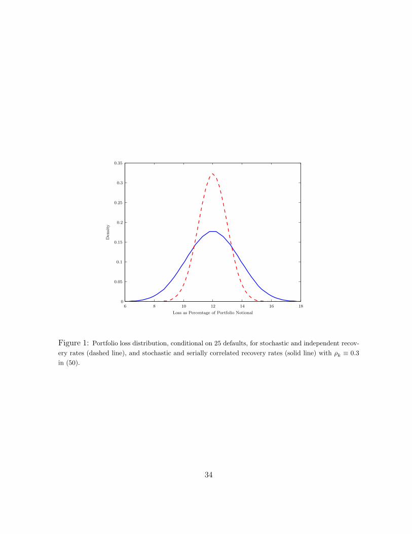
Figure 1 shows the portfolio loss distribution, conditional on 25 defaults, for thecase of (i) stochastic and (ii) stochastic and serially correlated recovery rates with samemarginal distribution of individual recovery rates. The parameters for the latter caseare ρk = 0.3 for 1 ≤ k ≤ m. We see that serial correlation of recovery rates leads tomuch fatter tails in the portfolio loss distribution, which is potentially good news froma modeling perspective.
33
0
0.05
0.1
0.15
0.2
0.25
0.3
0.35
6 8 10 12 14 16 18
Loss as Percentage of Portfolio Notional
Den
sity
Figure 1: Portfolio loss distribution, conditional on 25 defaults, for stochastic and independent recov-
ery rates (dashed line), and stochastic and serially correlated recovery rates (solid line) with ρk ≡ 0.3
in (50).
34

References
Altman, E., B. Bray, A. Resti, and A. Sironi (2005). The Link between Default andRecovery Rates: Theory, Empirical Evidence and Implications. Journal of Busi-ness 78, 2203–2227.
Altman, E. I. and V. M. Kishore (1996). Almost Everything You Wanted to Knowabout Recoveries on Defaulted Bonds. Financial Analysts Journal 52, 57–65.
Andersen, L., J. Sidenius, and S. Basu (2003). All your hedges in one basket. Risk ,67–72.
Berndt, A., R. Douglas, D. Duffie, M. Ferguson, and D. Schranz (2005). MeasuringDefault-Risk Premia from Default Swap Rates and EDFs. BIS Working Paper No.173.
Berndt, A., R. Jarrow, and C. Kang (2007). Restructuring Risk in Credit DefaultSwaps: An Empirical Analysis. Stochastic Processes and Their Applications 117,1724–1749.
Brigo, D. and A. Alfonsi (2004). Credit default swap calibration and derivatives pricingwith the SSRD stochastic intensity model. Finance and Stochastics 9, 29–42.
Burtschell, X., J. Gregory, and J. Laurent (2005). A comparative analysis of CDOpricing models. Working Paper, BNP-Paribas and University of Lyon.
Carr, P. and D. B. Madan (1999). Option Valuation Using the Fast Fourier Transform.Journal of Finance 2, 61–73.
Cerny, A. (2004). Introduction to Fast Fourier Transform in Finance. Journal ofDerivatives 12, 73–88.
’Credit Derivatives Handbook’ (2006). Merrill Lynch.
Das, S. S., D. Duffie, N. Kapadia, and L. Saita (2007). Common Failings: How Cor-porate Defaults are Correlated. Journal of Finance 62, 93–117.
Delbaen, F. and W. Schachermayer (1999). A General Version of the FundamentalTheorem of Asset Pricing. Mathematische Annalen 300, 463–520.
Ding, X., K. Giesecke, and P. Tomecek (2008). Time-Changed Birth Processes andMulti-Name Credit Derivatives. Forthcoming in Operations Research.
Driessen, J. (2005). Is Default Event Risk Price in Corporate Bonds. Review of Fi-nancial Studies 18, 165–195.
Duffie, D. (1999). Credit Swap Valuation. Financial Analysts Journal 55, 73–87.
Duffie, D., A. Eckner, G. Horel, and L. Saita (2009). Frailty Correlated Default.Journal of Finance 64, 2087–2122.
35

Duffie, D., D. Filipovic, and W. Schachermayer (2003). Affine Processes and Applica-tions in Finance. Annals of Applied Probability 13, 984–1053.
Duffie, D. and N. Garleanu (2001). Risk and Valuation of Collateralized Debt Obli-gations. Financial Analysts Journal 57, 41–59.
Duffie, D., J. Pan, and K. Singleton (2000). Transform Analysis and Asset Pricing forAffine Jump-Diffusions. Econometrica 68, 1343–1376.
Duffie, D. and K. Singleton (1997). An Econometric Model of the Term Structure ofInterest-Rate Swap Yields. Journal of Finance 52, 1287–1321.
Duffie, D. and K. Singleton (1999). Modeling Term Structures Of Defaultable Bonds.Review of Financial Studies 12, 687–720.
Duffie, D. and K. Singleton (2003). Credit Risk. Princeton, New Jersey: PrincetonUniversity Press.
Durrett, R. (2005). Probability: Theory and Examples (Third edition). Duxbury Ad-vanced Series.
Eckner, A. (2007). Risk Premia in Structured Credit Derivatives. Working Paper,Stanford University.
Errais, E., K. Giesecke, and L. R. Goldberg (2006). Pricing Credit from the Top Downwith Affine Point Processes.
Feldhutter, P. (2007). An Empirical Investigation of an Intensity-Based Model forPricing CDO Tranches. Working paper, Copenhagen Business School.
Feldhutter, P. and D. Lando (2004). Decomposing swap spreads. EFA 2006 ZurichMeetings.
Giesecke, K. and L. R. Goldberg (2005). A Top Down Approach to Multi-Name Credit.
Harrison, M. J. and D. Kreps (1979). Martingales and Arbitrage in Multiperiod Se-curities Markets. Journal of Economic Theory 20, 381–408.
Harrison, M. J. and S. R. Pliska (1981). Martingales and Stochastic Integrals in theTheory of Continuous Trading. Stochastic Processes and Their Applications 11,215–260.
Jackson, K., A. Kreinin, and X. Ma (2007). Loss Distribution Evaluation for SyntheticCDOs. Working paper, University of Toronto.
Jarrow, R. and S. Turnbull (1995). Pricing Options on Financial Securities Subjectto Default Risk. Journal of Finance 50, 53–86.
Joshi, M. and A. Stacey (2006). Intensity Gamma: A New Approach to Pricing Port-folio Credit Derivatives. Working paper, Royal Bank of Scotland.
36

Karatzas, I. and S. E. Shreve (2004). Brownian Motion and Stochastic Calculus (Sec-ond edition). Springer-Verlag.
Lando, D. (1998). On Cox Processess and Credit Risky Securities. Review of Deriva-tives Research 2, 99–120.
Li, D. (2000). On Default Correlation: A Copula Function Approach. Journal of FixedIncome 9, 43–54.
Longstaff, F. A. and A. Rajan (2008). An Empirical Analysis Of The Pricing OfCollateralized Debt Obligations. Journal of Finance 63, 529–563.
Lord, R. and C. Kahl (2006). Why the Rotation Count Algorithm Works. TinbergenInstitute Discussion Paper.
Moody’s (2000). Moody’s Investor Service: Historical Default Rates of CorporateBond Issuers, 1920-1999.
Mortensen, A. (2006). Semi-Analytical Valuation of Basket Credit Derivatives inIntensity-Based Models. Journal of Derivatives 13, 8–26.
Pan, J. and K. Singleton (2008). Default and Recovery Implicit in the Term Structureof Sovereign CDS Spreads. Journal of Finance 63, 2345–2384.
Papageorgiou, E. and R. Sircar (2008). Multiscale Intensity Models and Name Group-ing for Valuation of Multi-Name Credit Derivatives. Applied Mathematical Fi-nance 15, 73105.
Protter, P. (2005). Stochastic Integration and Differential Equations (Second edition).New York: Springer-Verlag.
Schneider, P., L. Sogner, and T. Veza (2009). The Economic Role of Jumps andRecovery Rates in the Market for Corporate Default Risk. Forthcoming in Journalof Financial and Quantitative Analysis.
37