Originally published as:

Balan, N., Zhang, Q.-H., Xing, Z., Skoug, R., Shiokawa, K., Lühr, H., Ram, S. T., Otsuka, Y., Zhao, L. (2019): Capability of Geomagnetic Storm Parameters to Identify Severe Space Weather. - The Astrophysical Journal, 887, 1, 51.

https://doi.org/10.3847/1538-4357/ab5113

1

1

2

Capability of Geomagnetic Storm Parameters to 3

Identify Severe Space Weather 4

5

N. Balan1,2, Qing-He Zhang1, Zanyang Xing1, R. Skoug3, K. Shiokawa4, 6

H. Lühr5, S. Tulasi Ram6, Y. Otsuka4, and Lingxin Zhao1 7

8

1Institute of Space Sciences, Shandong University, Weihai, Shandong 264209, China; 9

2Institute of Geology and Geophysics, Chinese Academy of Sciences, Beijing 100029, 10

China; 3Los Alamos National Laboratory, Los Alamos, NM 87544, USA 4Institute for 11

Space-Earth Environmental Research, Nagoya University, Nagoya 464-8601, Japan 12

5GFZ, German Research Centre for Geosciences, 14473 Potsdam, Germany. 6Indian 13

Institute of Geomagnetism, Navi Mumbai, 410218, India. 14

15

Correspondence to balan.nanan@yahoo.com 16

17

18

Running title: Severe space weather identification 19

20

Key words: Geomagnetic storm, IpsDst, severe space weather, solar wind and IMF 21

22

23

24

25

26

27

28

29

30

31

32

2

Abstract 33

34

The paper investigates the capability of geomagnetic storm parameters in Dst, Kp, and 35

AE indices to distinguish between severe space weather (SvSW) causing the reported 36

electric power outages and/or tele-communication failures and normal space weather 37

(NSW) not causing such severe effects in a 50-year period (1958-2007). The 38

parameters include the storm intensities DstMin (minimum Dst during the storm main 39

phase MP), (dDst/dt)MPmax, Kpmax, and AEmax. In addition, the impulsive parameter IpsDst 40

= (−1/TMP)∫TMP|DstMP|dt is derived for the storms automatically identified in Kyoto Dst 41

and USGS Dst. ∫TMP|DstMP|dt is the integral of the modulus of Dst from MP onset (MPO) 42

to DstMin. TMP is the MP duration from MPO to DstMin. The corresponding mean values 43

<KpMP> and <AEMP> are also calculated. Irrespective of the significant differences in the 44

storm parameters between the two Dst indices, the IpsDst in both indices seems 45

identifying 4 of the 5 SvSW events (and the Carrington event) from over 750 NSW 46

events reported occurring in 1958-2007, while all other parameters separate 1 or 2 47

SvSW from NSW. Using a Kyoto IpsDst threshold of -250 nT, we demonstrate a 100% 48

true SvSW identification rate with only one false NSW. Using the false NSW event 49

(1972 August 04), we investigate whether using a higher-resolution Dst might result in a 50

more accurate identification of SvSW. The mechanism of the impulsive action leading to 51

large IpsDst and SvSW involves the coincidence of fast ICME velocity V containing its 52

shock (or front) velocity △V and large IMF Bz southward covering △V. 53

54

1. Introduction 55

56

A series of rapid changes takes place in interplanetary space (IPS) and the environment 57

of planets during the passage of interplanetary coronal mass ejections (ICMEs) (e.g., 58

Witasse et al. 2017), high-speed streams, and CIRs (co-rotating interaction regions) 59

(Smith & Wolfe 1976). The changes are collectively called space weather. An ICME is a 60

huge, magnetized (interplanetary magnetic field IMF up to 100 nT), high density (up to 61

100 cm-3) plasma cloud ejected from the Sun and flowing out with speed up to 62

3

thousands of km s-1 (e.g., Skoug et al. 2004). However, the part of the ICME that is 63

most geoeffective is the magnetic cloud, which is a high magnetic field but low density 64

region (Burlaga et al. 1981). A high speed ICME produces shock waves ahead, which 65

accelerate the background charged particles to energies over 100 MeV, which are 66

known as solar energetic particles or SEPs (e.g., Singh et al. 2010). The particles are 67

accelerated to even higher energies by the high-speed ICME front that follows the ICME 68

shock (e.g., Balan et al. 2014). They can damage satellite systems (e.g., Green et al. 69

2017) and are harmful for biological systems, for example, astronauts (e.g., Aran et al. 70

2005). 71

72

In the Earth’s environment, space weather includes sudden changes (or disturbances) 73

in the magnetosphere, ring current, radiation belts, geomagnetic field, auroras, 74

ionosphere, and thermosphere. The disturbances in the geomagnetic field lasting from 75

several hours to several days and produced by the intensification of magnetospheric 76

current systems are called geomagnetic storms (Svalgaard 1977; Gonzalez et al. 1994; 77

Lühr, et al. 2017). The current systems contribute differently to the storms in different 78

latitudes; and the storms are therefore identified by the indices such as the low latitude 79

Dst (disturbance storm-time) index (Sugiura 1964; Love & Gannon 2009), mid latitude 80

Kp index, and high latitude AE index (e.g., Rostoker et al. 1995). Another index 81

sometimes used is the rate of change of the horizontal component (dH/dt) of the 82

geomagnetic field. The Dst storms arise mainly from the intensification of the ring 83

current due to ICME-magnetosphere coupling and ionosphere-ring current coupling, the 84

efficiency of which has been studied using solar wind and IMF data and models (e.g., 85

Burton et al. 1975; Fok et al. 2001; Newell et al. 2007; Leimohn et al. 2010). The storms 86

4

become more intense with the increase in the solar wind velocity V and strength of IMF 87

Bz southward (e.g., Ebihara et al. 2005). Based on the minimum value of Dst (DstMin) 88

reached during the storm main phase (MP), the storms are classified as moderate 89

storms (-100 <DstMin≤-50 nT), intense storms (−250 <DstMin≤-100 nT), and super 90

storms (DstMin ≤−250 nT) (e.g., Gonzalez et al. 1994). 91

92

Scientific analysis of solar storms and geomagnetic storms leads to fundamental 93

understanding of the Earth's surrounding space weather (e.g., Gopalswamy et al. 2005; 94

Kamide & Balan 2016). Application oriented analysis of the storms enables the 95

assessment and mitigation of space weather hazards on satellite systems, satellite 96

communication and navigation, electric power grids, tele-communication systems, etc. 97

Of particular concern are the effects associated with extreme storms (e.g., Boteler 2001; 98

Viljanen et al. 2010; Hapgood 2011; Pulkkinen 2007; Love et al. 2017). A space 99

weather event similar to the Carrington event of 1859 September 01-02 (Carrington 100

1859) occurring at the present times could cause very serious impacts in today’s high-101

tech society (e.g., Baker 2008; Schrijver et al. 2015; Eastwood et al. 2017). It is 102

therefore important for both scientific and technological reasons to identify some 103

parameters of the storms that can indicate their severity. 104

105

Conventionally, DstMin, maximum rate of change of Dst during MP (dDst/dt)MPmax, and 106

maximum values of Kp and AE (Kpmax and AEmax), all representing geomagnetic storm 107

intensities, have been used for investigating the space weather in Earth’s environment. 108

However, while studying what determines the severity of the space weather (Balan et 109

al., 2014) we realized that DstMin is an insufficient indicator of severe space weather 110

(SvSW), as reported also by Cid et al. (2014). We define severe space weather 111

5

(SvSW) as causing the reported electric power outages and/or tele-communication 112

failures and normal space weather (NSW) as not causing such severe effects in a 50-113

year period (1958-2007). Our studies also showed that the mean value of Dst during 114

MP (⟨DstMP⟩) can indicate the severity of space weather (Balan et al. 2016). ⟨DstMP⟩ can 115

also be used as a better reference than DstMin in developing a scheme for forecasting 116

SvSW using ICME velocity and magnetic field (Balan et al. 2017a). The derived 117

parameter (⟨DstMP⟩) will hereafter be called IpsDst (Section 2). 118

119

In the brief report (Balan et al. 2016), we introduced IpsDst indicating the impulsive (Ips) 120

strength of Dst storms to distinguish between SvSW and NSW using only the super 121

storms (DstMin ≤-250 nT) in Kyoto Dst data. No other data were used. The present 122

paper investigates the capability of the important storm parameters in Dst, Kp, and AE 123

indices to distinguish between the SvSW and NSW events reported occurring in a 50-124

year period (1958-2007). In addition to the conventional parameters mentioned above, 125

the paper uses the IpsDst for the Dst storms automatically identified in the widely used 126

Kyoto Dst and new (and improved) USGS Dst data in 1958-2007. The paper also uses 127

the mean values of Kp and AE during MP (<KpMP> and <AEMP>) in the same 50-year 128

period. The SvSW events include the event on 1972 August 04, which was missed in 129

Balan et al. (2016) because it occurred during a non-super storm (DstMin -125 nT). It 130

has puzzled the scientific community because all other SvSW events (including the 131

Carrington event of 1859 September 01-02) occurred during super storms. The paper 132

also explains the physical significance of IpsDst and discusses the physical mechanism 133

leading to large IpsDst and SvSW using the solar wind and IMF data from the ACE 134

(Advanced Composition Explorer) satellite available since 1998. 135

6

136

Section 2 describes the data and analysis. The results are presented and discussed in 137

Sections 3 and 4. The SvSW events reported occurring in the 50-year period (1958-138

2007) and the Carrington SvSW event only are investigated. The SvSW events reported 139

occurring prior to the Dst era (Davidson 1940; Cliver & Dietrich 2013; Ribeiro et al. 2016; 140

Love & Coïsson 2016; Love 2018) are discussed in Section 4, though not investigated 141

for the lack of Dst data. Minor technological problems such as capacitor stripping in 142

power transformers (e.g., Kappenman 2003) will be included later by using high 143

resolution IpsDst. 144

145

2. Data and Analysis 146

147

148

Figure 1. Scatter plot of hourly Kyoto Dst against USGS Dst in 1958-2007. 149

150

The hourly Kyoto Dst and USGS Dst data covering a 50-year time period (1958-2007) 151

are available at http://wdc.kugi.kyoto-u.ac.jp/dstdir/ and http://geomag.usgs.gov/data, 152

7

respectively. The primary difference between the Kyoto Dst (Sugiura 1964; Sugiura & 153

Kamei 1991) and USGS Dst (Love & Gannon 2009) is in the removal of secular and 154

solar quiet (Sq) variations. Kyoto Dst partially removes these variations while USGS Dst 155

more fully removes them, which results in an offset between the two indices. Love & 156

Gannon (2009) presented a panoramic view of the two indices for the whole 50-year 157

period and detailed comparisons for selected 40-day time segments. They reported 158

significant offset (Kyoto minus USGS) of up to -70 nT between the indices. Figure 1 159

shows a scatter plot of the indices in the 50-year period. The indices have a correlation 160

of 0.96 and the offset is mainly negative. The average offset is -8.50 nT in all data 161

together and -5.0 nT in quiet-time (Dst >-25 nT) data alone (Balan et al. 2017b). For the 162

Carrington storm, the H-component data measured at Bombay (Tsurutani et al. 2003) 163

and calculated by Cliver & Dietrich (2013) are used. The Kp and AE data are available 164

at http://wdc.kugi.kyoto-u.ac.jp/kp/index.html and http://wdc.kugi.kyoto-u.ac.jp/aedir/, 165

respectively. 166

167

The Dst storms were automatically identified by a computer program that uses four 168

selection criteria. The criteria are (1) DstMin ≤ -50 nT and TMP > 2 hours, (2) absolute 169

value of MP range, that is, |DstMPO -DstMin| ≥ 50 nT, (3) separation between DstMin and 170

next MPO ≥ 10 hours, and (4) rate of change of Dst during MP or (dDst/dt)MP <-5 nT/hr. 171

MPO here stands for MP onset. The selection criteria minimize non-storm like 172

fluctuations (Balan et al. 2017b). The computer program identified 761 storms in Kyoto 173

Dst, which include 34 super storms, 296 intense storms, and 431 moderate storms. The 174

8

175

Figure 2. Comparison of four super storms (DstMin ≤-250 nT) in Kyoto Dst (blue) and USGS 176

Dst (red) having large IpsDst (purple shade) and comparatively weak IpsDst (yellow shade). 177

MPOs are identified by a computer program satisfying storm selection criteria and IMF Bz 178

turning southward. The time T0 of X-axis corresponds to 12 UT on 2003 October 28 (panel a), 179

2001 November 05 (panel b), and 2003 November 19 (panel c), respectively. 180

181

585 storms identified in USGS Dst include 33 super storms, 210 intense storms, and 182

342 moderate storms. Figure 2 compares four super storms in the two indices. Intense 183

and moderate storms were compared before (Balan et al. 2017b). Although the storms 184

in the two indices exhibit similar variations, they have differences in DstMin and in its 185

time of occurrence, which can cause differences in IpsDst. 186

187

9

2.1. Parameter IpsDst 188

189

The parameter IpsDst is defined as IpsDst = (−1/TMP)∫TMP|DstMP|dt (Balan et al. 2014). 190

∫TMP|DstMP|dt is the integral (or sum) of the modulus of Dst from MPO to DstMin. MPO is 191

the MP onset time when Dst starts decreasing satisfying the storm selection criteria 192

(and IMF Bz turning southward) which is also the peak of the storm sudden 193

commencement (SSC). TMP is the time interval (or duration) from MPO to DstMin. The 194

rate of change of Dst during the MP and its maximum value (dDst/dt)MPmax are obtained. 195

By definition, the IpsDst includes most important characteristics of Dst storms (SSC, 196

MPO, (dDst/dt)MPmax, DstMin, and TMP) and gives the mean value of Dst during the MP 197

when most energy input occurs (Figure 2). IpsDst is proportional to the total amount of 198

energy input during MP (e.g., Burton et al. 1975) divided by the duration of energy input. 199

The higher the energy input and shorter the duration, the larger the IpsDst value and 200

more impulsive its action, and so the name IpsDst. The maximum values of the Kp and 201

AE storms (Kpmax and AEmax) are noted. Their MP durations corresponding to the MP of 202

Dst storms are identified as shown by an example in Figure 3. The mean values of Kp 203

and AE during the storm MP are calculated as 204

⟨KpMP⟩ = ΣKpMP/TMP and ⟨AEMP⟩ = ΣAEMP/TMP. 205

206

⟨KpMP⟩ and ⟨AEMP⟩ might represent the impulsive strength of the Kp and AE storms 207

because they give the mean values of Kp and AE during the storm MP when most 208

energy input occurs. 209

The accuracy of IpsDst depends on the accuracy of the Dst data and TMP. According to 210

Sugiura (1964), who developed the Dst index, it is not easy to compute the uncertainty 211

of Dst (T. Iyemori 2019, private communication). The uncertainty includes the 212

10

213

Figure 3. An example identifying the storm main phase MP in Dst, Kp, and AE storms. 214

measurement errors at the four Dst observatories, errors associated with the selection 215

of 5 quiet days for each month, and errors due to the variation of quiet-time ring current 216

when Dst is zero. These errors are mostly removed in the final version of Dst especially 217

in USGS Dst (Love & Gannon 2009). The uncertainty also seems to depend on the time 218

when a storm actually hits the Dst stations and the time when Dst shows the storm. 219

However, this difference in time may not cause significant difference in Dst because the 220

ring current starts developing not at a specific point in time but during a certain range in 221

time (M. Nose 2019, private communication). The accuracy of TMP depends on the 222

accurate identification of the times of MPO and DstMin. The computer program 223

identifies these times following the selection criteria. The MPO times of the storms since 224

1998, when ACE data are available, are also found agreeing with the times of IMF Bz 225

turning southward. The time resolution (1 hour) of the Dst data, however, can cause 226

significant uncertainty in IpsDst. It causes ±30 minutes uncertainty in the identification of 227

MPO and DstMin or an uncertainty ΔTMP of ±1 hour in TMP. The corresponding 228

11

uncertainty in IpsDst is ΔIpsDst = ±IpsDstx(ΔTMP/TMP). Table 1 lists the computed 229

IpsDst and its uncertainty of all 35 super storms and the intense storm on 1972 August 230

04. It assumes that the uncertainty in Dst is negligible compared to that in TMP. The 231

uncertainty in general decreases with increasing (negative) IpsDst. 232

233

Figure 4. Scatter plot of the absolute and percentage differences (Kyoto minus USGS) in 234

DstMin (a and b) and IpsDst (c and d) of the storms in the two Dst indices as function of time, 235

with red color for super storms and blue color for intense and moderate storms together. The 236

average differences are noted inside brackets. 237

12

238

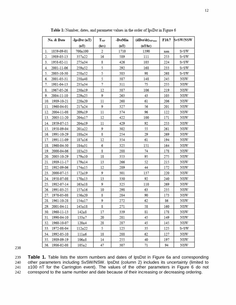
Table 1. Table lists the storm numbers and dates of IpsDst in Figure 6a and corresponding 239

other parameters including SvSW/NSW. IpsDst (column 2) includes its uncertainty (limited to 240

±100 nT for the Carrington event). The values of the other parameters in Figure 6 do not 241

correspond to the same number and date because of their increasing or decreasing ordering. 242

13

243

The offset between the two Dst indices causes differences in their storm parameters. 244

Figure 4 shows the absolute and percentage differences (Kyoto minus USGS) in DstMin 245

and IpsDst of the storms as function of time, with red color for super storms and blue 246

color for intense and moderate storms together. Though the absolute difference is 247

mainly negative up to -54 nT in DstMin (Figure 4a) and -58 nT in IpsDst (Figure 4c), it is 248

also positive up to 20 nT in DstMin and 84 nT in IpsDst for a small number of storms. 249

The percentage difference is positive up to 40% in DstMin (Figure 4b) and 65% in 250

IpsDst (Figure 4d) though it is negative up to -35% in DstMin and -130% in IpsDst for a 251

small number of storms. The average differences noted in the figure are smaller in 252

IpsDst than DstMin by about 2 nT on the whole, though their percentage differences are 253

nearly equal. TMP (not shown) is found equal for about half of the storms and differs for 254

others resulting in an average difference of -0.28 hours overall. TMP differs generally due 255

to the DstMin in one index occurring slightly later or earlier compared to the other index 256

(Figure 2). As discussed, there are significant offsets between the two Dst indices and 257

differences in their storm parameters. It therefore becomes interesting to investigate 258

how well the various important storm parameters in the two Dst indices and Kp and AE 259

indices work in distinguishing between the SvSW and NSW events. 260

The ACE satellite at the L1 point has provided IMF and solar wind data continuously 261

since 1998. The velocity and density data in the SWI (Solar Wind Ion) mode of the 262

SWEPAM (Solar Wind Electron Proton Alpha Monitor) instrument at 64-second 263

resolution (e.g., McComas et al. 1998; Skoug et al. 2004) are available at Caltech 264

(http://www.srl.caltech.edu/ACE/ASC/). During high energy particle events, when the 265

14

SWI mode may not cover the full solar wind flux distribution, the 64-second data 266

collected in the SSTI (Search/Supra Thermal Ion) mode once every ~32 minutes will be 267

used. The data (time) is corrected for the ACE-Earth distance. The velocity and IMF 268

data for the Carrington, Quebec, 1958 February, and 1972 August events are adopted 269

from the calculations by Cliver & Svalgaard (2004), Nagatsuma et al. (2015), Cliver et 270

al. (1990), and Vaisberg & Zastenker (1976), respectively. 271

272

For discussing the mechanism connecting the Dst storms and solar storms (Section 273

4.3), we define the beginning of an ICME event as the time when the solar wind velocity 274

(V) suddenly increases to high values (Balan et al. 2014). The ICME event front (or 275

shock) velocity ΔV is the difference between the peak ICME velocity and the upstream 276

slow solar wind velocity (V). The velocity, especially during severe events measured 277

with 32-minute resolution, is found to take about two hours to reach its peak. ΔV in 278

general is therefore taken as the difference between the mean velocity for 2 hours after 279

and 2 hours before the start of the velocity increase. Bz at ΔV (BzΔV) is the mean of Bz 280

for the two hours from the start of the velocity increase. 281

282

3. Identification of SvSW 283

284

3.1. Definition and events 285

286

As mentioned in Section 1, the space weather events reported to have caused electric 287

power outages and/or telegraph system failures in the 50-year period (1958-2007) are 288

defined as severe space weather (SvSW). Five such SvSW events are reported 289

occurring in 1958-2007. The event of 1958 February 11 damaged telegraph systems in 290

Sweden (e.g., Wik et al. 2009) and caused electric power supply problems in the US 291

15

292

Figure 5. Scatter plot of IpsDst against DstMin of the Carrington storm and all common storms 293

during 1958-2007 in (a) Kyoto Dst and (b) USGS Dst. Red and green dots correspond to SvSW 294

events. Regions 1-2 and 2-3 represent the IpsDst ranges of NSW and SvSW events including 295

the uncertainty in IpsDst due to the uncertainty in TMP of the respective highest and lowest 296

IpsDst values. The horizontal bars show the uncertainty in IpsDst of the SvSW events only for 297

simplicity and limited to ±100 nT for the Carrington event. 298

299

(Slothower & Albertson 1967). The event of 1972 August 04 caused tele-communication 300

failure and electric power supply problems in the US (Anderson et al.1974; Albertson & 301

Thorson 1974). The Quebec event of 1989 March 13 (e.g., Medford et al. 1989) and the 302

New Zealand event of 2001 November 06 (Marshall et al. 2012) caused electric power 303

16

outages. The Halloween event of 2003 October 30 caused an electric power outage in 304

Sweden (e.g., Pulkkinen et al. 2005). The Carrington event of 1859 September 01-02 305

that caused telegraph system failures (Loomis 1861) is also included. All other space 306

weather events occurred in the 50-year period are considered normal space weather 307

(NSW) events because they are not reported to have caused such severe effects. 308

309

3.2. Identification 310

311

Using DstMin and IpsDst, we attempt to determine their abilities to differentiate between 312

SvSW and NSW events for each of the two Dst indices. Figure 5 shows scatter plots of 313

IpsDst against DstMin considering all common storms in 1958-2007. For the Carrington 314

storm (right-hand top event), the equivalent DstMin and IpsDst are limited to -650 nT 315

and -450 nT, respectively. Red and green colors represent SvSW in Kyoto Dst and 316

USGS Dst, respectively. The regions marked 1-2 and 2-3 represent the IpsDst ranges 317

of NSW and SvSW events including the uncertainty in IpsDst due to the uncertainty in 318

TMP of the respective highest and lowest IpsDst values. IpsDst, seems able to mostly 319

differentiate between the populations of SvSW and NSW in both Dst indices. Using 320

DstMin only allows for the separation of 2 out of the 6 events. Due to the lone SvSW 321

event (1972 August 04) that is not separated by IpsDst, there appears a very wide 322

range of IpsDst that can cause SvSW and the distribution overlaps with that of NSW. 323

We will discuss the 1972 August 04 SvSW event in Section 4.1. 324

325

Next, we include other important storm parameters. Though we analysed all storms, the 326

parameters are shown only for all super storms, the intense storm of 1972 August 04, 327

and the Carrington storm. Figure 6 displays the IpsDst, TMP, DstMin, and (dDst/dt)MPmax 328

17

329

Figure 6. IpsDst, TMP, DstMin, (dDst/dt)MPmax, and F10.7 on the days of DstMin of the super 330

storms (DstMin ≤-250 nT) in Kyoto Dst arranged in their increasing or decreasing orders. The 331

Carrington storm of 1859 and intense storm on 1972 August 04 are included. Red color 332

corresponds to SvSW and blue color to NSW (see text). 333

334

18

in Kyoto Dst; the solar activity index F10.7 on the days of DstMin is also shown. For the 335

Carrington event (number 1), the equivalent DstMin, IpsDst, and (dDst/dt)MPmax are 336

limited to -650 nT, -450 nT, and 200 nT/hr, respectively, for better display with other 337

parameters in the figure. All parameters are arranged in their respective increasing or 338

decreasing orders. Red and blue colors represent SvSW and NSW events, respectively. 339

Table 1 lists the IpsDst together with its uncertainty and other parameters for each of 340

the storms shown in Figure 6. IpsDst best sorts out SvSW from NSW, despite the 341

outlier of event number 33 (1972 August 04) having significantly weak IpsDst (-112 nT), 342

which will be discussed in Section 4.1. 343

344

Figure 7 is similar to Figure 6 but for USGS Dst with green and black colors 345

representing SvSW and NSW events, respectively. The offset between the two Dst 346

indices results in the absence of one super storm in USGS Dst. The differences in the 347

respective storm parameter values between the two indices result in some differences 348

in the order number of the parameters in Figure 7 compared to Figure 6. For these 349

reasons, F10.7 is also shown in Figure 7. The behavior of all parameters in USGS Dst 350

is similar to that in Kyoto Dst. 351

3.3. Kp and AE indices 352

353

Since SvSW effects usually occur at high latitudes, one might expect the high and mid 354

latitude indices (AE and Kp) could also be used to distinguish between SvSW and NSW 355

events. However, these indices are inadequate as illustrated in Figure 8, which shows 356

⟨KpMP⟩, Kpmax, ⟨AEMP⟩, and AEmax corresponding to the Dst storms in Figure 6a. The 357

parameters are arranged in their respective decreasing orders. Red and blue colors 358

359

19

360

Figure 7. IpsDst, TMP, DstMin, (dDst/dt)MPmax, and F10.7 on the days of DstMin of the super 361

storms (DstMin ≤-250 nT) in USGS Dst arranged in increasing or decreasing orders of the 362

parameters. The Carrington storm of 1859 and intense storm on 1972 August 04 are included. 363

Green color corresponds to SvSW and black color to NSW (see text). 364

365

20

366

367

368

Figure 8. ⟨KpMP⟩, Kpmax, ⟨AEMP⟩x10-2, and AEmaxx10-2 arranged in their decreasing orders. The 369

parameters correspond to the Dst storms shown in Figure 6a. The Carrington event has no Kp 370

data and five events including the Carrington and 1972 August 04 events have no AE data. Red 371

and blue colors correspond to SvSW and NSW, respectively. 372

373

correspond to SvSW and NSW, respectively. In Figure 8a, the SvSW events from left to 374

right correspond to the storms in 2001 November, 2003 October, 1958 February, 1989 375

March, and 1972 August, respectively. The Carrington event has no Kp data and five 376

events including the Carrington and 1972 August 04 events have no AE data. In all 377

parameters (Figure 8), the SvSW events are mixed with NSW events. AE and Kp seem 378

inadequate to distinguish between SvSW and NSW mainly because they do not 379

21

distinguish their phases when a majority of energy input occurs. Kp is also a 3-hour 380

index, and AE can sometimes reach maximum before the main energy input starts from 381

the MPO of Dst storms. 382

383

4. Discussion 384

385

As mentioned in Section 1, Dst storms have been studied and modeled for many years 386

using Dst index, solar wind, and IMF data. The models have improved our 387

understanding of the mechanisms connecting Dst storms and solar storms. For 388

example, using V, N (density), and Bz, Burton et al. (1975) modeled the seven Dst 389

storms in 1967–1968. Klimas et al. (1997) presented a method for transforming a linear 390

prediction model into linear and non-linear dynamical analogues of the coupling 391

between the input and output data. Using VBz for input and Dst for output, they showed 392

that the non-linear analogue couples to the solar wind through the expression 393

(VBz/Dst)×VBz rather than through the usual linear dependence on VBz. The multi-input 394

(VBz and dynamic pressure P) and single-output (Dst) discrete time model developed 395

by Zhu et al. (2007) explains the Dst dynamics more accurately than previous models. 396

Using USGS Dst and a lognormal stochastic process, Love et al. (2015) reported that 397

the most extreme Dst storms (DstMin ≤ -850 nT) can occur ~1.13 times per century, 398

with 95% confidence level. The ICME-magnetosphere coupling function developed by 399

Newell et al. (2007) is a good measure of the coupling efficiency, though is still not able 400

to distinguish between SvSW and NSW (Balan et al. 2017a). 401

402

By definition, the parameter IpsDst = (−1/TMP)∫TMP|DstMP|dt gives the mean value of Dst 403

duirng storm MP (Figure 2), and therefore indicates the impulsive strength of Dst storms 404

22

Table 2：Truth table 405

Total = 762 Identified

True False

Actual SvSW a = 5 b = 0

Actual NSW c = 756 d = 1

406

Table 2: The truth table lists the number of (a) true SvSW, (b) false SvSW, (c) true NSW, and 407

(d) false NSW events identified by IpsDst for a threshold of -250 nT in Kyoto Dst. 408

409

(IpsDst). The important result from Section 3 is that, irrespective of the significant offset 410

and differences between the two Dst indices, the impulsive parameter IpsDst in both 411

indices seems more likely to distinguish between SvSW and NSW events than other 412

common Dst-based parameters. Using a truth table, we calculate the success of the 413

identification. Table 2 lists the number of (a) true SvSW, (b) false SvSW, (c) true NSW, 414

and (d) false NSW identified by IpsDst for a threshold of -250 nT in Kyoto Dst. Following 415

Kohavi & Provost (1998), we calculate an accuracy [(a+c)/(a+b+c+d)] of 99.9% for the 416

identification of SvSW and NSW events together and a true SvSW identification rate 417

[a/(a+b)] of 100% with only one false NSW. The false NSW corresponds to the event on 418

1972 August 04 having small IpsDst, which is actually a SvSW event (Figure 5). We 419

discuss this event in greater detail below. 420

421

4.1. SvSW Event on 1972 August 04 422

423

As reported by Anderson et al. (1974) and Albertson & Thorson (1974), a 424

communication cable system outage and electric power supply problems occurred in 425

the US during the rapid changes in the magnetic field during the large geomagnetic 426

storm on 1972 August 04. Though no solar wind and IMF data were available, 427

measurement of the time delay between the solar flare onset and shock arrival at 1 AU 428

23

gives the fastest ever recorded speed of ~2850 km s-1 for the ICME shock (Vaisberg & 429

Zastenker 1976) which might have compressed the magnetopause to ~5Re (Anderson 430

et al. 1974; Lanzerotti 1992). Study of the Pioneer 10 data at ~2 AU showed that the 431

average IMF Bz was around zero with considerable north-south fluctuations, and the 432

geomagnetic storm was probably caused by a southward Bz fluctuation following the 433

fast ICME shock (Tsurutani et al. 1992). The calculations by Tsurutani et al. (1992), 434

assuming a solar wind speed of 2000 km s-1 and magnetopause compression to 5Re, 435

show large storm-time ring current peak intensity corresponding to -295 nT. Kp reached 436

its highest values of 9; AE data are not available. Model calculations by Boteler & Beek 437

(1999) showed that the outages were due to a rapid intensification of the electrojet 438

current as is typical for other SvSW events. The high impulsive action of the fastest 439

ICME shock followed by the short-duration Bz southward seems to account for this 440

SvSW event. If Bz had been southward for a longer period covering the ICME shock or 441

ICME front, this event could have caused devastating effects. 442

443

The Dst storm (Figure 9d) has MPO at 23 UT (Dst -45 nT in Kyoto Dst) and DstMin 444

(-125 nT) at 04 UT giving a TMP of 5 hours and IpsDst of -112 nT, which is low 445

compared to the IpsDst of other SvSW events. The hourly values of the corresponding 446

H components (Figure 9c) used for calculating Dst also have low H ranges (△H = 52-92 447

nT) though their durations (1-2 hours) are short compared to TMP (5 hours). To better 448

understand the IpsDst value, the H component magnetograms at the Dst stations 449

Kakioka and San Juan available at http://wdc.kugi.kyoto-u.ac.jp/film/index.html are 450

manually scaled four times at 5-minute intervals. The scaled values are digitized using 451

24

452

Figure 9. Scaled values (5-minute resolution) of the H component magnetograms on 1972 453

August 04-05 at the Dst stations (a) Kakioka and (b) San Juan with standard deviations; zero 454

corresponds to baseline levels of 30094 nT and 27440 nT, respectively. The corresponding (c) 455

hourly H values at all four Dst stations used for computing the (d) Dst index are shown. 456

Important parameter values are listed. 457

458

25

the baseline values of 30094 nT and 27440 nT, respectively, and scale conversion 459

factors provided by the observatories (M. Nose, 2018, private communication). The 4 H 460

values at each time step are used to obtain their mean and standard deviation (up to 461

~15%). The time variations of H (Figures 9a and 9b) show large △H over very short 462

durations (315 nT in 45 minutes at Kakioka and 215 nT in 40 minutes at San Juan) 463

translating to △HK of 420 nT and △HS of 325 nT in 1 hour. The △H values are used to 464

calculate Dst (Sugiura & Kamei, 1991) as Dst = (1/2)(△HK/cos(26.0)+△HS/cos(29.9)) 465

with 26.0 and 29.9 being the dip latitudes at Kakioka and San Juan. It gives 1-hour Dst 466

(and IpsDst) of ~-421 nT. This is an approximate value because we could not use the 467

magnetograms at Honolulu and Hermanus, which have poor quality, and could not 468

apply the Sq correction, which requires H values for previous five years. 469

470

To check the effect of high resolution data further, we use the SymH index available 471

since 1981 at http://wdc.kugi.kyoto-u.ac.jp/aeasy to calculate IpsSymH. It is similar to 472

IpsDst but calculated for the SymH index of 1-minute resolution derived using the H 473

component data from 12 low latitude stations (Iyemori et al. 1991). The distribution of 474

IpsSymH (not shown) is similar to that of IpsDst (Figure 5); and it appears that IpsSymH 475

may be superior to IpsDst in its ability to distinguish between SvSW and SNW. Further 476

studies using high resolution Dst (at least since 1958) are required to calculate the 477

likelihood that a given IpsDst will actually cause SvSW or NSW, which is planned as 478

described below. 479

4.2. SvSW Events Prior to Dst era 480

481

In addition to the SvSW events in 1958-2007 and the Carrington event investigated in 482

Section 3, the SvSW events reported occurring prior to the Dst era also seem to agree 483

26

with the criterion of large IpsDst. Love (2018) reported widespread problems that 484

occurred in telegraph and telephone systems in the US on 1882 November 17. The 485

simultaneous magnetograms recorded at the nearby station Los Angeles (40.88˚N 486

magnetic) showed a 1-hour average △H of 470 nT, TMP of 5 hours, and large dH/dt. 487

Using Bombay magnetograms, they (Love 2018) estimated a DstMin of -386 nT. The aa 488

index, which is a simple 3 hourly global geomagnetic activity index available since 1868 489

and derived from two approximately antipodal observatories in Australia and UK 490

(Mayaud 1972), averaged to its highest value of 215 nT. These characteristics indicate 491

a large IpsDst (<-250 nT). Ribeiro et al. (2016) described widespread problems 492

occurring in the telegraph communication networks in two mid-latitude countries 493

(Portugal and Spain) on 1903 October 31. The magnetic field recorded simultaneously 494

in these countries showed a large storm (similar to the Quebec storm of 1989 March 13) 495

with H ranges over 500 nT and large dH/dt indicating that the corresponding IpsDst 496

could have been <-250 nT. As reviewed by Cliver & Dietrich (2013), the event on 1921 497

May 14-15 caused telephone cable burning in Sweden and a fire at the Central New 498

England Railroad Station switchboard in the US. Based on simultaneous 499

magnetograms, Kappenman (2006) estimated DstMin ~-850 nT for this storm, which 500

indicates a large IpsDst. The magnetic storms on 1940 March 24 and 1941 September 501

19 which caused electric power supply and tele-communication problems in the US 502

(Davidson 1940 and Love & Coïsson, 2016) and when Kp reached 9 are also estimated 503

to have large IpsDst and DstMin (<-250 nT) (unpublished Dst data, J. J. Love 2018, 504

private communication). 505

We plan to digitize the analogue magnetograms available since 1904 at the four Dst 506

27

stations at high time resolution (e.g., 5-minutes), compute the Dst data, automatically 507

identify the Dst storms, and obtain the IpsDst and other important storm parameters. 508

The magnetograms available at Cape Town will be used for the period prior to 1940 509

when the same are not available for the closest Dst station Hermanus. We will study 510

how well the high-resolution storm parameters work in identifying the reported SvSW 511

events including minor technological problems since 1904. We expect that the high 512

resolution IpsDst will enable us calculate the likelihood that a given IpsDst will actually 513

cause SvSW or NSW. In short, the high resolution IpsDst could be a very useful 514

parameter for investigating different aspects of space weather. 515

516

4.3. Physical Mechanism 517

518

The mechanism of large IpsDst (high energy input over a short duration) probably takes 519

place through continuous and rapid magnetic reconnection (e.g., Borovsky et al. 2008). 520

This important physical process seems to happen when there is a simultaneous 521

occurrence of high solar wind velocity V (>~700 km s-1) coupled with a high ICME front 522

velocity ΔV (sudden increase by over 275 km s-1) and sufficiently large IMF Bz 523

southward during the velocity increase ΔV (Balan et al. 2014). The importance of the 524

coincident velocity increase and IMF Bz southward is illustrated in Figure 10. It displays 525

the IpsDst of the 13 super storms (in Kyoto Dst) since 1998, Carrington super storm, 526

and 1972 August 04 storm (number 15) and corresponding ICME and IMF drivers in 527

increasing order of IpsDst. The ⟨VMP⟩ of the Carrington and 1972 August 04 SvSW 528

events is limited to 1600 km s-1 and their △V is limited to 1200 km s-1. The solar wind 529

velocity and IMF Bz data for the Carrington, Quebec, 1958 February, and 1972 August 530

events (numbers 1-3 and 15) are adopted from the theoretical calculations by Cliver & 531

28

532

Figure 10. IpsDst of the super Dst storms (Kyoto Dst) since 1998, Carrington storm (number 1), 533

and 1972 August storm (number 15) and corresponding ⟨VMP⟩x⟨BzMP⟩, ⟨VMP⟩, ⟨BzMP⟩, △V, and 534

Bz△V obtained from ACE data and adopted from theoretical values available in the literature (see 535

text). All parameters are arranged in increasing order of IpsDst with red color for SvSW. 536

537

29

Svalgaard (2004), Nagatsuma et al. (2015), Cliver et al. (1990), and Vaisberg & 538

Zastenker (1976), respectively. An IMF Bz of -10 nT is assumed for the 1972 August 04 539

event following Tsurutani et al. (1992). 540

541

The red histograms correspond to SvSW and blue histograms to NSW. As shown, 542

IpsDst has (nearly) the same distribution as the product ⟨VMP⟩x⟨BzMP⟩ (Figures 10a and 543

10b) except for the event number 15 (1972 August 04) due to its high <VMP>. The 544

SvSW events 1-5 and 15 have both high ⟨VMP⟩ (Figure 10c) and large ⟨BzMP⟩ southward 545

(Figure 10d), as well as high ΔV (Figure 10e) and BzΔV southward during the time of 546

large ΔV (Figure 10f). Their combined action leads to large IpsDst. ⟨BzMP⟩ southward 547

opens the dayside magnetopause and high ΔV (and high ⟨VMP⟩) provides the force for 548

the impulsive entry of a large number of high-energy charged particles into the 549

magnetosphere and ring current. For NSW events (blue), the product ⟨VMP⟩x⟨BzMP⟩ is 550

comparatively small. Their striking difference compared to SvSW events is small ΔV 551

(except for the events 9 and 14) and Bz generally northward at the time of ΔV, so that 552

either their impulsive action is weak or the strong action becomes ineffective. The 553

coincidence of high ⟨VMP⟩ with high ΔV and simultaneous large ⟨BzMP⟩ southward 554

leading to a steep decrease of Dst and large IpsDst was modeled (Balan et al. 2017a) 555

using the CRCM (comprehensive ring current model) of Fok et al. (2001). The model 556

also showed that a high ⟨VMP⟩ not associated with a large ΔV and large ⟨BzMP⟩ 557

southward does not lead to large IpsDst. In Figure 10, the 1972 August 04 SvSW event 558

is identified by ⟨VMP⟩x⟨BzMP⟩ but not by IpsDst because IMF Bz remained southward 559

only for a short duration less than 1 hour as discussed in Section 4.1. It is also worth 560

noting that while IpsDst is useful for identifying SvSW in ground data, the solar 561

30

parameter VxBz showing a sharp negative spike exceeding a threshold is useful for 562

forecasting SvSW with a maximum warning time of ~35 minutes using ACE satellite 563

data (Balan et al. 2017a). 564

565

The coherence of the global parameters (high ΔV and large Bz southward) leading to 566

another global parameter (large IpsDst) and a regional phenomenon (SvSW) reveals an 567

impulsive solar wind-magnetosphere-ionosphere coupling, which seems essential for 568

SvSW (Figure 10). The impulsive coupling results in an intense regional ionospheric 569

current somewhere at high latitudes (e.g., Boteler & Beek, 1999), which generates 570

strong magnetic fields reaching down to earth, which, in turn, induce strong currents 571

and voltages in Earth systems (e.g., Viljanen et al. 2010). Such induced currents and 572

voltages exceeding the tolerance limits of the systems cause system failures (e.g., 573

Albertson et al. 1974; Lanzerotti 1983). Finally, it should be mentioned that the global 574

parameter IpsDst can do only its job of identifying SvSW and it cannot indicate the time 575

and location of the system damages that depend also on the regional ionospheric and 576

ground conductivities and characteristics of the systems (power girds and tele-577

communication networks). 578

579

Summary 580

581

1. The parameter IpsDst = (−1/TMP)∫TMP|DstMP|dt gives the mean value of Dst during the 582

storm MP. Its value decreases with increasing energy input (∫TMP|DstMP|dt) and 583

decreasing duration of energy input (TMP), and therefore indicates the impulsive 584

strength of Dst storms while DstMin and (dDst/dt)MPmax represent only their intensity 585

at a single point in time. 586

31

587

2. IpsDst captures many important processes (ICME shock, magnetopause 588

compression, SSC and energy input) related to the physical mechanism (high 589

energy input over a short duration) causing the sudden intensification of high latitude 590

ionospheric currents leading to severe space weather (SvSW) resulting in electric 591

power outages and tele-communication system failures. 592

593

3. IpsDst is derived for the Dst storms automatically identified in Kyoto Dst and USGS 594

Dst data for a period of 50 years (1958-2007). The IpsDst in both indices seems 595

distinguishing 4 of the 5 SvSW events (and the Carrington event) from over 750 596

NSW events occurred in 1958-2007 though the indices have significant offset of up 597

to -70 nT in Dst and differences of up to -54 nT in DstMin and -58 nT in IpsDst. The 598

storm parameters DstMin, (dDst/dt)MPmax, AEmax, Kpmax, <AEMP>, and <KpMP> can 599

identify only 1 or 2 of the SvSW events. Using an IpsDst threshold of -250 nT in 600

Kyoto Dst, we demonstrate a 100% true SvSW identification rate with only one false 601

NSW. 602

603

4. The lone SvSW event occurred during a non-super storm on 1972 August 04 that 604

appears low impulsive in Dst data (has a low value of IpsDst) is identified as a false 605

NSW. Actually, it is also highly impulsive as revealed by the large H ranges (420 nT 606

and 325 nT) of short durations (1 hour) observed in the available magnetograms at 607

two Dst stations. The results indicate that it may be useful to consider high resolution 608

IpsDst in the future. 609

610

5. The mechanism of large IpsDst is investigated using the solar wind velocity V and 611

IMF Bz measured by the ACE satellite since 1998. The mechanism involves the 612

32

coincidence of high ⟨VMP⟩ containing a high ICME front velocity △V (sudden increase 613

by over 275 km s-1) and large ⟨BzMP⟩ southward covering △V. Their combined 614

impulsive action can cause impulsive entry of a large amount of high-energy 615

charged particles into the magnetosphere and ring current through continuous and 616

rapid magnetic reconnection leading to large IpsDst and SvSW, through impulsive 617

solar wind-magnetosphere-ionosphere-ground system coupling. 618

619

Acknowledgments 620

621

We thank the referee of this paper for the critical comments and helpful suggestions that 622

have improved the quality of the paper. He/she deserves to be a co-author. We also 623

thank M. Nose and T. Iyemori of Kyoto University (WDC) for the scientific discussions and 624

magnetograms on 1972 August 04-05 recorded at the Dst observatories at Kakioka, San Junn, 625

Honolulu, and Hermanus which are available at http://www.kakioka-jma.go.jp/en/index.html, 626

https://geomag.usgs.gov/ and http://www.sansa.org.za/spacescience, respectively. We 627

acknowledge the use of Kyoto Dst and USGS Dst data available at http://swclob-kugi.kyoto-628

u.ac.jp and http://geomag.usgs.gov/data), and SymH index available at http://wdc.kugi.kyoto-629

u.ac.jp/aeasy. This research was supported by the National Key R&D Program of China 630

(2018YFC140730，2018YFC1407303), the National Natural Science Foundation of 631

China (grants 41604139, 41574138, 41774166, 41431072, 41831072), the Chinese 632

Meridian Project, the foundation of National Key Laboratory of Electromagnetic 633

Environment (grants 6142403180102, 6142403180103), and JSPS KAKENHI 634

(15H05815 and 16H06286) in Japan. Work at Los Alamos was performed under the 635

auspices of the U.S. Department of Energy with support from the NASA-ACE program. 636

637

638

639

References 640

641

Albertson, V. D. & Thorson, J. M. 1974 IEEE Trans Power App&Sys PAS-93 1025 642

643

Albertson, V. D., Thorson,J. M. & Miske, S. A. 1974 IEEE Trans Power App&Sys PAS-93 1031 644

33

645

Anderson, C.W., Lanzerotti, L. J. & Maclennan, C. G. 1974 BellSys Tech J 53 1817 646

647

Aran, A., Sanahuja, B., & Lario, D. 2005 AnnGeophys 23 doi:10.5194/angeo-23-3047-2005. 648

649

Baker, D. N. et al. 2008 1-144 The National Academy Press, Washington, DC, 1-144 650

651

Balan, N., Skoug, R., TulasiRam, S., Rajesh, P. K., Shiokawa, K., Otsuka, Y., Batista, I. S., 652

Ebihara Y., & Nakamura T. 2014 JGR 119 doi:10.1002/2014JA020151 653

654

Balan, N., Batista, I. S., TulasiRam, S. & Rajesh, P. K. 2016 Geoscience Letters 3.3 655

doi:10.1186/s40562-016-0036-5 656

657

Balan, N., Ebihara, Y., Skoug, R., Shiokawa, K., Batista, I. S., TulasiRam, S., Omura, Y., 658

Nakamura, T., & Fok, M.-C. 2017a. JGR 122, doi:10.1002/2016JA023853 659

660

Balan, N., TulasiRam, S., Kamide, Y., Batista, I. S., Souza, J. R., Shiokawa, K., Rajesh, P. K., & 661

Victor, N. J. 2017b EPS, 69:59, doi10.1186/s40623-017-0642-2 662

663

Boteler, D. H. 2001 AGU Geophysical Monograph 125 347-352 664

665

Boteler, D.H., & Beek, G. J. 1999 GeoRL 26 577 666

667

Borovsky, J. E., Hesse, M., Birn, J., & Kuzentsova, M. M. 2008 JGR 113 A07210 668

669

Burlage, L., Sittler, E., Mariani, F., & Schwenn, R. 1981 JGR 86 6673-6684 670

671

Burton, R. K., McPherron, R. L., & Russell, C. T. 1975 JGR 80 4204 672

673

Carrington, R. C. 1859 Mon. Not. R. Astron. Soc. 20 13 674

675

Cid. C., Palacios, J., Saiz, E., Guerrero, A., & Cerrato, Y. 2014 JSWSC 4 A28 676

doi:10.1051/swsc/2014026 677

678

Cliver, E. W., Feynman, J., & Garrett, H. B. 1990 JGR 95 17103 679

680

Cliver, E. W., & Svalgaard, L. 2004 SoPh 224 407 681

682

Cliver, E. W., & Dietrich, W. F. 2013 3 A31, doi:10.1051/swsc/2013053. 683

684

Davidson, W.F. 1940 Edison Electric Institute Bulletin July. 685

686

Eastwood, J. P., et al. 2017 Risk Analysis 37 (2) 206 687

688

Ebihara, Y., et al. 2005 JGR 110, A09S22 689

690

Fok, M.-C., Wolf, R. A., Spiro, R. W., & Moore, T. E. 2001 JGR 106 8417 691

34

692

Gonzalez, W. D, Joselyn, J. A., Kamide, Y., Kroehl, H. W., Rostoker, G., Tsurutani, T. B., & 693

Vasyliunas, V. M. 1994 JGR, 99, 5771 694

695

Gopalswamy, N., Yashiro, S., Michalek, G., Xie, H., Lepping, R. P., & Howard, R. A. 2005 696

GeoRL doi:10.1029/2004GL021639 697

698

Green, J. C., Likar, J. & Shprits, Y. 2017 SpWea 15 804 699

700

Iyemori, T., Araki, T., Kamei, T., & Takeda, M. 1992 No. 1 1989, Data Anal. Center for 701

Geomagn. and Space Magn., Kyoto Univ., Japan. 702

703

Hapgood, M. A. 2011 AdSpR 47, 2059 704

705

Kamide, K., & Balan, N. 2016 Geoscience Letters 3:10 https://doi.org/10.1186/s40562-016-706

0042-7. 707

708

Kappenman, J., G. 2003 SpWea 1 NO. 3, 1016 709

710

Kappenman, J. G. 2006 AdSpR 38(2) doi.org/10.1016/j.asr.2005.08.055. 711

712

Klimas, A. J., Vassiliadis, D., & Baker, D. N. 1997 JGR 102 26993 713

714

Kohavi, R., & Provost, F. 1998 On Applied Research in Machine Learning 30 Columbia 715

University New York 716

717

Lanzerotti, L. J. 1983 SSRv 34 347 718

719

Lanzerotti, L., J. 1992 Geo. Physics. Res. 19 19 720

721

Liemohn M. W., Jazowski, M., Kozyra, J. U., Ganushkina, N., Thomsen, M. F., & Borovsky, J. E. 722

2010 Proc. R. Soc. A 466 3305 723

724

Love, J. J., & Gannon, J. L. 2009 AnGeo 28(8) 3101 725

726

Love, J. J., Rigler, E. J., Pulkkinen, A., & Riley, P. 2015 GeoRL 42 6544 727

728

Love, J. J., & Coïsson, P. 2016 1941 Eos 97 doi:10.1029/2016EO059319 729

730

Love, J. J., Lucas, G. M., Kelbert, A., & Bedrosian, P. A. 2017 GeoRL doi: 731

10.1002/2017GL076042 732

733

Love, J. J. 2018, SpWea, 16 doi.org/10.1002/2017SW001795. 734

735

Lühr, H., Xiong, C., Olsen, N., & Le, G. 2017 SSRv 206 521–545 736

737

35

Marshall, R. A., Dalzell, M., Waters, C. L., Goldthorpe, P., & Smith, E. A. 2012 SpWea 10 738

S08003, doi:10.1029/2012SW000806 739

740

Mayaud, P. N. 1972 JGR 77 6870-6874 741

742

McComas, D. J., Bame, S. J., Barker, P., Feldman, W. C., Phillips, J. L., & Riley, P. 1998 SSRv 743

86 563 744

745

Medford et al. 1989 GoRL 16(10) 1145 746

747

Nagatsuma, T., Kataoka, R., & Kunitake, M. 2015 EPS 67:78 doi:10.1186/s40623-015-0249-4. 748

749

Newell, P. T., Sotirelis, T., Liou, K., Meng, C.-I., & Rich, F. J. 2007 JGR 112 A01206 750

doi:10.1029/2006JA012015 751

752

Pulkkinen, T. 2007 Living Rev Solar Phys 4 1 753

754

Pulkkinen, A., Lindahl, S., Viljanen, A., & Pirjola, R. 2005 SpWea 3 S08C03 755

doi:10.1029/2004SW000123 756

757

Ribeiro, P., Vaquero, J. M., Gallego, M. C., & Trigo, R. M. 2016 SpWea 14 758

doi:10.1002/2016SW001424. 759

760

Rostoker, G., Samson, J. C., Creutzberg, F., Hughes, T. J., McDiarmid., D. R., McNamara, A. 761

G., Vallance Jones, A., Walls, D. D., & Cogger, L. L. 1995 SSRv 46 743 762

763

Schrijver, C. J., et al. 2015 AdSpR 55(12) 2745 764

765

Singh, A. K., Devendra Singh, & Singh, R. P. 2010 SurvGeophys 31 581 766

767

Skoug, R. M., Gosling, J. T., Steinberg, J. T., McComas, D. J., Smith, C. W., Ness, N. F., Hu, 768

Q., & Burlaga, L. F. 2004 JGR 109 A09102 769

770

Slothower, J.C., & Albertson, V. D. 1967 J Minn Academy Science 34 94 771

772

Smith, E. J., & Wolfe, J. H.1976 Geo Physics Res 3 137 773

774

Sugiura, M. 1964 Ann. Int. Geophysical Year, 35 9-45 Pergamon New York 775

776

Sugiura, M., & Kamei, T. 1991 IAGA Bull. 40, Int Serv of Geomagn Indices Saint-Maur-des-777

Fosses France 778

779

Svalgaard L. 1977 edited by J. B. Zirker 371–441 Colo Assoc Univ Press Boulder 780

781

Tsurutani, B. T., Gonzaez, W. D., Tang, F., Lee, Y. T., Okada, M., & Park, D. 1992 GoRL 19 782

1993 783

784

36

Tsurutani, B. T., Gonzalez, W. D., Lakhina, G. S., & Alex, S. 2003 JGR 108 1268 785

786

Vaisberg, O.L., & Zastenker, G. N. 1976 SSRv 19 687 787

788

Viljanen, A., Koistinen, A., Pajunpää, K., Pirjola, R., Posio P., & Pulkkinen, T. 2010 Geophysica 789

46 59 790

791

Viljanen, A., Pirjola, R., Pracser, E., Ahmadzai, S., & Sing, V. 2013 SpWea 11 575 792

793

Witasse et al. 2017 JGR 122 7865 794

795

Wik, M., Pirjola, R., Lundstedt, H., Viljanen, A., Wintoft, P., & Pulkkinen, A. 2009 AnGeo 796

27 1775 797

798

Zhang, R., Liu, L., Le, H., Chen, Y., & Kuai, J. 2017 JGR 122. 799

https://doi.org/10.1002/2017JA024637 800

801

Zhu., D., Billings, S. A., Balikhin, M. A., Wing, S., & Alleyne, H. 2007 JGR 112 A06205 802

803

Table and Figure captions 804

805

Table 1. Table lists the storm numbers and dates of IpsDst in Figure 6a and corresponding 806

other parameters including SvSW/NSW. The values of the other parameters in Figure 6 do not 807

correspond to the same number and date because of their increasing or decreasing ordering. 808

809

Table 2: The truth table lists the number of (a) true SvSW, (b) false SvSW, (c) true NSW, and 810

(d) false NSW events identified by IpsDst for a threshold of -250 nT in Kyoto Dst. 811

812

Figure 1. Scatter plot of hourly Kyoto Dst against USGS Dst in 1958-2007. 813

Figure 2. Comparison of four super storms (DstMin ≤-250 nT) in Kyoto Dst (blue) and USGS 814

Dst (red) having large IpsDst (purple shade) and comparatively weak IpsDst (yellow shade). 815

MPOs are identified by a computer program satisfying storm selection criteria and IMF Bz 816

turning southward. The time T0 of X-axis corresponds to 12 UT on 2003 October 28 (panel a), 817

2001 November 05 (panel b), and 2003 November 19 (panel c), respectively. 818

Figure 3. An example identifying the storm main phase MP in Dst, Kp, and AE storms. 819

820

Figure 4. Scatter plot of the absolute and percentage differences (Kyoto minus USGS) in 821

DstMin (a and b) and IpsDst (c and d) of the storms in the two Dst indices as function of time, 822

with red color for super storms and blue color for intense and moderate storms together. The 823

average differences are noted inside brackets. 824

Figure 5. Scatter plot of IpsDst against DstMin of the Carrington storm and all common storms 825

during 1958-2007 in (a) Kyoto Dst and (b) USGS Dst. Red and green dots correspond to SvSW 826

events. Regions 1-2 and 2-3 represent the IpsDst ranges of NSW and SvSW events including 827

the uncertainty in IpsDst due to the uncertainty in TMP of the respective highest and lowest 828

37

IpsDst values. The horizontal bars show the uncertainty in IpsDst of the SvSW events only for 829

simplicity and limited to ±100 nT for the Carrington event. 830

Figure 6. IpsDst, TMP, DstMin, (dDst/dt)MPmax, and F10.7 on the days of DstMin of the super 831

storms (DstMin ≤-250 nT) in Kyoto Dst arranged in their increasing or decreasing orders. The 832

Carrington storm of 1859 and intense storm on 1972 August 04 are included. Red color 833

corresponds to SvSW and blue color to NSW (see text). 834

835

Figure 7. IpsDst, TMP, DstMin, (dDst/dt)MPmax, and F10.7 on the days of DstMin of the super 836

storms (DstMin ≤-250 nT) in USGS Dst arranged in increasing or decreasing orders of the 837

parameters. The Carrington storm of 1859 and intense storm on 1972 August 04 are included. 838

Green color corresponds to SvSW and black color to NSW (see text). 839

840

Figure 8. ⟨KpMP⟩, Kpmax, ⟨AEMP⟩x10-2, and AEmaxx10-2 arranged in their decreasing orders. The 841

parameters correspond to the Dst storms shown in Figure 6a. The Carrington event has no Kp 842

data and five events including the Carrington and 1972 August 04 events have no AE data. Red 843

and blue colors correspond to SvSW and NSW, respectively. 844

845

Figure 9. Scaled values (5-minute resolution) of the H component magnetograms on 1972 846

August 04-05 at the Dst stations (a) Kakioka and (b) San Juan with standard deviations; zero 847

corresponds to baseline levels of 30094 nT and 27440 nT, respectively. The corresponding (c) 848

hourly H values at all four Dst stations used for computing the (d) Dst index are shown. 849

Important parameter values are listed. 850

851

Figure 10. IpsDst of the super Dst storms (Kyoto Dst) since 1998, Carrington storm (number 1), 852

and 1972 August storm (number 15) and corresponding ⟨VMP⟩x⟨BzMP⟩, ⟨VMP⟩, ⟨BzMP⟩, △V, and 853

Bz△V obtained from ACE data and adopted from theoretical values available in the literature (see 854

text). All parameters are arranged in increasing order of IpsDst with red color for SvSW. 855

856

857