balance sheets, exchange rate policy, and welfare - imf.org · balance sheets, exchange rate...
TRANSCRIPT
WP/04/63 Revised: 5/13/04
Balance Sheets, Exchange Rate Policy, and Welfare
Selim Elekdag and Ivan Tchakarov

© 2004 International Monetary Fund WP/04/63 Revised: 5/13/04
IMF Working Paper
Middle East and Central Asia Department and Research Department
Balance Sheets, Exchange Rate Policy, and Welfare
Prepared by Selim Elekdag and Ivan Tchakarov1
Authorized for distribution by Saade Chami and Gian Maria Milesi-Ferretti
April 2004
Abstract
This Working Paper should not be reported as representing the views of the IMF. The views expressed in this Working Paper are those of the author(s) and do not necessarily represent those of the IMF or IMF policy. Working Papers describe research in progress by the author(s) and are published to elicit comments and to further debate.
The debate about the appropriate choice of exchange rate regime is fundamental in international economics. This paper develops a small open-economy model with balance sheet effects and compares the performance of fixed and flexible exchange rate regimes. The model is solved up to a second-order approximation which allows us to address the issue of risk and welfare rigorously. The paper identifies threshold levels of the debt-to-GDP ratio above which fixed exchange rate regimes are welfare superior to monetary policy rules that imply flexible exchange rate regimes. The results suggest that emerging market economies that suffer from a relatively high level of indebtedness and are constrained in their pursuit of optimal monetary policy, could find it beneficial to opt for a fixed exchange rate regime. JEL Classification Numbers: F31, F41 Keywords: Exchange rate policy, financial accelerator, debt-to-GDP threshold, second-order
approximation Author’s E-Mail Address: [email protected]; [email protected]
1 Selim Elekdag is with the IMF’s Middle East and Central Asia Department and Ivan Tchakarov is with the IMF’s Research Department. The authors thank Tamim Bayoumi, Roberto Chang, Woon Gyu Choi, Gian Maria Milesi-Ferretti, Simon Gilchrist, Michael Devereux, and Douglas Laxton for useful comments and discussions. Susanna Mursula has been very helpful in developing the procedures used in the model simulations.
- 2 -
Contents Page I. Introduction...................................................................................................................3 II. Model................. ...........................................................................................................6 A. Representative Household ......................................................................................6 B. Production Firms ....................................................................................................8 C. Entrepreneurs ..........................................................................................................9 D. Central Bank .........................................................................................................10 E. Market Clearing.....................................................................................................11 F. Solution Methodology ...........................................................................................12 G. Computation of the Welfare Measure...................................................................12 III. Results.........................................................................................................................14 A. Export Demand Shock ...........................................................................................14 B. Welfare Analysis ....................................................................................................15 IV. Concluding Remarks ..................................................................................................19 Tables: 1. Parameter Calibration ...............................................................................................21 2. Regime Comparison..................................................................................................22 3. Detailed Regime Comparison ...................................................................................23 4. Alternative Regime Comparison ..............................................................................24 5. Comparisons with Other Regimes and Calibrations ..... ...........................................25 Figures: 1. Negative Export Shock under a Peg (No Financial Accelerator) .............................26 2. Negative Export Shock under a Float (No Financial Accelerator) ...........................27 3. Negative Export Shock under a Peg (with Financial Accelerator) ...........................28 4. Negative Export Shock under a Float (with Financial Accelerator) ........................29 5. Welfare Comparison using a First-Order Approximation ..... ..................................30 6. Welfare Comparison using a Second-Order Approximation....................................31 7. Emerging Market Bonds Index ................................................................................32 8. Alternative Welfare Comparison using a First-Order Approximation ..... ...............33 9. Alternative Welfare Comparison using a Second-Order Approximation ................34 References..........................................................................................................................35

- 3 -
I. INTRODUCTION
After the severe �nancial crises that erupted in East Asia, the question of appropriate monetarypolicy for emerging market economies has received renewed attention. The common policyprescription that dates back to Friedman (1953) has advocated the implementation of �exibleexchange rate regimes. A freely �oating nominal exchange rate has the ability to act as a shockabsorber and insulate the economy against external shocks. In a model with nominal rigidities,by allowing the currency to depreciate, the monetary authority facilitates a smoother adjustmentrelative to a �xed exchange rate regime.
However, emerging market economies are faced with two fundamental issues that complicatethe conduct of monetary policy. First, these countries typically can only borrow in foreigncurrency denominations, a phenomenon called �Original Sin� by Eichengreen and Hausman(1999). Second, they are subject to a risk premium above and beyond the international lendingrate. This premium in turn depends on the amount of collateral invested towards the project. Thecombination of these features that is referred to as the �nancial accelerator, collateral constraintsor the balance sheet channel, creates a �nancially vulnerable environment.2 A sudden depreciationin�ates liabilities that are denominated in foreign currency, thus reducing the value of collateralthat can be used towards investment projects. As collateral evaporates, the risk premium that mustbe endured increases substantially, thus choking off the process of capital accumulation. This isone reason why many monetary authorities in emerging market economies have been reluctantto allow the currencies to �oat freely, and this is consistent with the �Fear of Floating� argumentadvanced by Calvo and Reinhart (2001). Even though a depreciation can potentially boost exportvolumes by promoting competitiveness, it can also trigger a potentially severe recession due tobalance sheet effects and collateral constraints.
The incorporation of the �nancial accelerator channel has been introduced in a dynamic generalequilibrium setting by Cespedes, Chang, and Velasco (2001, 2002); Devereux and Lane (2003);and Gertler, Gilchrist, and Natalucci (2003). These authors have made an important contributionto extending macroeconomic analysis to emerging market economies by incorporating balancesheet effects and collateral constraints in a standard small open-economy framework. The mainconclusion of this line of research is consistent with the conventional wisdom embodied in theMundell-Fleming framework, which promotes the implementation of �exible exchange rateregimes. This result is upheld even when such �nancial frictions are present in the model. A �oatcan insulate the economy against adverse external shocks more effectively than a peg by allowingthe currency to depreciate. The general consensus in these papers is that only in calibrationsyielding "extreme" values of fundamentals can a peg be better than a �oat.
While the above literature has been instrumental in developing models that explicitly accountfor balance sheet effects, it has been limited to comparing the relative performance of �xed and�exible exchange rates by only investigating impulse response functions. For example, Cespedes,
2 We use the terms �nancial accelerator, collateral constraints, and balance sheet effectsinterchangeably in our analysis.

- 4 -
Chang and Velasco (2002) contrast the behavior of different exchange rate regimes when theeconomy is subject to foreign interest rate and export shocks. Cespedes, Chang and Velasco(2001) recognize the limitations of this approach and construct an ad-hoc loss function. Whiletheir model is based on �rm microfoundations, it is somewhat unsettling that they use a welfaremetric that does not derive from �rst principles. Devereux and Lane (2003) conduct welfareanalysis but ignore the effects of risk on the behavior of economic agents.3
In these models the consequences of uncertainty on welfare are impossible to analyze accurately.The main reason for this is the fact that researchers have typically resorted to linearizationtechniques to approximate the model and have, therefore, abstracted from higher moments. Itis obvious then that, in a linear environment, it is impractical to ask the question if risk plays asigni�cant role in affecting households' decisions. This stems from the fact that when a modelis linearized, certainty equivalence holds, which does not allow agents to explicitly incorporaterisk in their decision-making process. This seems to be much more important in a model wherethe main purpose is to account for the behavior of the risk premium associated with borrowingfrom abroad, and to analyze how economic agents change their decisions based on the capacity ofdifferent exchange rate regimes to mitigate such risks.
The main objective of this study is to conduct a welfare-based comparison of �xed and �exibleexchange rate regimes. Our analysis builds on the model of Cespedes, Chang, and Velasco (2001,2002), but carries out a rigorous welfare examination of this issue. This is made possible by asolution algorithm which can deal with second-order approximations to the equilibrium conditionsof stochastic models. As has been emphasized by Cespedes, Chang, and Velasco (2001), the taskof addressing these questions �...is not trivial, since there are a number of distortions (�nancialfrictions in addition to sticky prices and monopoly power) and therefore Taylor approximationsto the social objective function may not always yield the quadratic forms we have relied on.� Insuch an environment a linear-quadratic approach, where one employs a quadratic approximationof the utility function, but evaluates it only with a linear approximation of the model equations,may lead to potentially spurious welfare results as has been emphasized by Kim and Kim (2003).Woodford (2001) has also shown that the usually employed linear approximations describing theequilibrium behavior of the model will represent a correct welfare ranking of alternative policyregimes only under very restrictive assumptions. The latter will not be met in any reasonably richgeneral equilibrium model, such as the one developed below.
While the balance sheet transmission mechanism has been found to provide useful insights inthe debate about the appropriate choice of exchange rate regime, not much has been exploredempirically about its quantitative implications. In this respect, another objective of this paperis to analyze quantitatively the relevance of this mechanism in explaining output behavior inthe aftermath of a devaluation. For this purpose, we augment the model proposed by Cespedes,Chang, and Velasco ( 2002) by incorporating a monetary sector in terms of an interest rate rule,mutli-period price stickiness, a richer menu of �nancial assets, and introducing an economy-wide
3 This is because Devereux and Lane (2003) use a welfare metric that is not completelyaccurate since it is based on a linear-quadratic approach. See below for further details.

- 5 -
technology shock in line with the real business cycle literature.
The main �ndings can be summarized as follows. We verify that a policy of strict in�ationtargeting is better than a �xed exchange rate from a welfare point of view in a world where the�nancial accelerator is not present, which serves to reinforce the policy recommendations of theMundell-Fleming framework. Also, consistent with previous literature, welfare costs are higherin a model with the �nancial accelerator present, relative to the one without it for both �xed and�exible exchange rate regimes.
When the �nancial accelerator is present, we identify threshold values of the debt-to-GDP ratioabove which the peg becomes superior to the �oat in terms of welfare. These thresholds are verysensitive to the approximation method. When we use a linear approximation, it is only when debtis above 31 percent of GDP that a �exible exchange rate delivers lower welfare. However, whenwe solve the model using a second-order approximation, properly account for the uncertaintyinherently present in our framework, and conduct the welfare analysis correctly, the thresholddrops to a much more plausible value of 16 percent.
The main message of this paper is to treat with caution the results obtained by the previousliterature that consider collateral constraints and employ welfare metrics that are not rigorous.Not only do we demonstrate an accurate method of conducting welfare analysis, but much moreimportantly, we show that one can simulate cases where a peg dominates a �oat for a wide rangeof debt levels.4
We also provide different robustness checks that support the overall message of the paper. Similarresults are obtained using versions of the Taylor rule, different degrees of the intratemporalelasticity of substitution between home and foreign goods, and varying degrees of openness.
Our results do not necessarily imply that �xed exchange rates are universally superior to �exibleexchange rates. It is possible to entertain the case that optimally calibrated interest-rate rules thatentail high exchange rate �exibility may yield higher welfare than a peg even for debt-to-GDPratios of above 16 percent. In this sense, our analysis should not be viewed as an attempt tochange the conventional policy recommendations prescribed by the Mundell-Fleming model.
At the same time, we believe that our results are useful in providing insights into the behaviorof emerging market economies. If monetary authorities in such countries have to deal withmacroeconomic imbalances in an environment characterized by weak institutional capacity, thena conscious policy of pursuing optimal behavior may be desirable, but dif�cult to achieve. Inthis respect, Hunt, Isard, and Laxton (2002) argue that optimal policy rules can be very sensitiveto model speci�cations and, therefore, "...it could be dangerous for monetary authorities to useoptimal rules as guidelines for policy."
4 Devereux (2004) provides an example of a model without balance sheet effects wherea cooperative peg dominates a �oat. Choi and Cook (2004) develop a model with a banking systemthat operates in a similar fashion to the entrepreneurial sector, which also advocates a �xed exchange rate regime.

- 6 -
The remainder of the paper is organized as follows. Section II lays out the model, Section IIIdescribes the results and Section IV concludes.
II. MODEL
Our basic modeling framework is an extension of Cespedes, Chang, and Velasco (2002), where wefocus on a small open economy with a representative household, producers, entrepreneurs, and acentral bank. The economy produces a composite consumption good and imports a foreign good.The domestic good is a bundle that is composed of a continuum of goods produced by domestic�rms in a monopolisitically competitive environment. These �rms each supply a differentiatedgood and hence enjoy market power, which they exploit to maximize their pro�ts. This warrantsactive cyclical monetary policy. To this end, we incorporate a central bank that uses an interest raterule to achieve speci�c policy objectives. The representative household is allowed to accumulate�nancial assets and is thus responsive to interest rate �uctuations.
A. Representative Household
The household is in�nitely lived and its preferences are de�ned over aggregate consumption, Ct,and labor effort, Lt, which are described by the following utility function:
E0
1Xt=0
�t
"C1��t
1� �� �
L1+ t
1 +
#(1)
where Et denotes the mathematical expectation conditional on information available in period t,and � 2 (0; 1) is the subjective discount factor.
Aggregate consumption is a bundle consisting of a domestically produced good and an importedforeign good:
Ct = �C HtC
1� Ft (2)
where CHt denotes the consumption of the home good, CFt consumption of the imported good,and � = [ (1� )1� ]�1 is a normalizing constant.
Following Cespedes, Chang and Velasco (2002), we assume that the price of the imported goodis normalized to unity in terms of foreign currency. Also, imports are assumed to be freely tradedand the Law of One Price holds, so that the domestic currency price of imports is just equal tothe nominal exchange rate St. The aggregate price level, Qt, is then derived by solving for theminimum expenditure required to obtain one unit of the aggregate consumption good. Denotingthe price of the of the domestic good as Pt, the aggregate price level it then:
Qt = P t S
1� t (3)
- 7 -
Given the aggregate price index, the individual consumption demands for each good can bederived:
CHt =
�PtQt
��1Ct (4)
CFt = (1� )
�StQt
��1Ct (5)
The domestic good is itself a composite good, consisting of a CES aggregate of the continuum ofdifferentiated domestic goods, more speci�cally:
CHt =
�ZC
��1�
Hjt dj
� ���1
(6)
where j 2 [0; 1] and � > 1. Each unique good CHjt; is produced by a monopolisticallycompetitive �rm. This gives each �rm market power which motivates price stickiness.
The household's budget constraint in period t is as follows:
QtCt +Qt�t +Bt+1 + StF�t+1 = WtLt +�t + (1 + it�1)Bt + (1 + i�t�1)StF
�t (7)
where Bt+1 and F �t+1 are nominal stocks of domestic and foreign currency denominated bondsmaturing in period t, which earn interest it�1 and i�t�1 respectively.5 Households earn wageWt fortheir labor services Lt. Since they own the domestic production �rms, they retain any pro�ts, �t.Finally, households must incur an intermediation cost, �t, which has the following speci�cation:
�t =�B2
�Bt+1
Qt
�2+�F �
2
�StF
�t+1
Qt
�2(8)
where �B; �F � > 0 and �B + �F � > 0:Without this cost, the stocks of bonds and consumptionwould not be stationary, preventing the model from being solved using the Sims (2000) method.
The household chooses the paths of fCt; Lt; Bt; F�t g1t=0 to maximize its expected lifetime utility
(1) subject to the constraint (7) and initial values for B0 and F0. Ruling out Ponzi-type schemes,we get the following �rst-order conditions:
5 It is important to note that, as is common in the literature, we too assume that Bt+1and F �t+1 are zero in the non-stochastic steady state.

- 8 -
�L tC��t
=Wt
Qt
(9)
C��t [1 + �BBt+1] = �(1 + it)Et[C��t+1
Qt
Qt+1
] (10)
C��t [1 + �F �StF�t+1] = �(1 + i�t )Et[C
��t+1
Qt
Qt+1
St+1St] (11)
The �rst condition implies that the household equates its marginal rate of substitution betweenconsumption and leisure to the real wage, Wt=Qt. The last two �rst-order conditions are thefamiliar Euler equations which emphasize the household's preference to smooth consumption.Abstracting from the intermediation costs, they can be combined to yield the familiar uncoveredinterest parity condition.
B. Production Firms
The economy is populated by a multitude of monopolistically competitive �rms each producing aunique good. The production technology for an arbitrary �rm j 2 [0; 1] is:
Yjt = AtK�jtL
1��jt (12)
where, At, is the technology shock common to all production �rms. The household provides thelabor services and capital,Kjt; is provided by the entrepreneurs to be described below. Production�rms exploit their market power and set prices in order to maximize pro�ts along a downwardsloping demand curve given by:
Yjt =
�PjtPt
���Yt (13)
Following Rotemberg (1982), we assume that it is costly to adjust prices because of quadraticmenu costs. Hence, an arbitrary �rm maximizes the discounted stream of pro�ts given by:
E0
1Xt=0
�t;t+1 [Pjt �MCt � ACjt]Yjt (14)
where the quadratic price adjustment cost ACjt and marginal costMCt are de�ned as:
- 9 -
ACjt ='
2
(Pjt � Pj;t�1)2
Pj;t�1(15)
MCt =R�tW
1��t
At��(1� �)1��(16)
Firms are owned by the household, hence the present future value of pro�ts are discountedaccording to the household's intertemporal marginal rate of substitution in consumption, whichimplies:
�t;t+1 = �C��t+1C��t
Qt
Qt+1
(17)
The pro�t maximization problem implies a trade-off between capital and labor inputs that dependson the relative cost of each of them, and price setting behavior:
�RtKt = (1� �)WtLt (18)
1 = �
"1� MCt
Pjt� '
2
(Pjt � Pj;t�1)2
Pj;t�1
#� '
2Et
��
�P 2jt+1P 2jt
� 1�Yjt+1Yjt
�+ '
�Pjt+1Pjt
� 1�(19)
Equation (19) is a New Keynesian Phillips' curve which reverts to the familiar mark-up rule whenthere are no adjustment costs (' = 0):
Pjt =�
�� 1MCt (20)
C. Entrepreneurs
One of our main objectives in this paper is to analyze the consequences of balance sheet effectsin the simplest framework possible. Therefore we adapt the structure introduced by Cespedes,Chang, and Velasco (2002) when introducing the �nancial accelerator in an open economycontext. Although the inclusion of entrepreneurs is crucial to our investigation, we provide onlya concise presentation and refer the reader to the work of Cespedes, Chang, and Velasco (2002)along with Bernanke, Gertler, and Gilchrist (2000) for further details.
Entrepreneurs �nance investment partly with foreign loans subject to frictions. In any given
- 10 -
period, the entrepreneur is assumed to have some net worth denominated in domestic currency.When the entrepreneur engages in capital accumulation and the investment outlays exceed networth, the entrepreneur must �nance the remainder by borrowing foreign currency denominatedassets from abroad. Hence the entrepreneur is subject to the following budget constraint:
PtNt = QtKt+1 � StD�t+1 (21)
where, Nt and D�t+1; denote net worth and foreign currency denominated debt, respectively. It is
important to notice that net worth is equal to assets minus foreign currency denominated liabilities.This highlights one channel by which net worth is susceptible to exchange rate �uctuations.
Entrepreneurs are risk neutral and choose D�t+1 and Kt+1 to maximize pro�ts. We assume that
capital depreciates completely in production. Due to informational asymmetries, the expectedreturn to investment is equal to the foreign interest rate augmented by a risk premium �t+1, that is:
Et
�Rt+1Kt+1=St+1QtKt+1=St
�= (1 + i�t+1)(1 + �t+1) (22)
Bernanke, Gertler and Gilchrist (2000) show that the risk premium can be expresses as anincreasing function of the value of investment relative to net worth:
(1 + �t+1) =
�QtKt+1
PtNt
�(23)
where (�) = 1: and (�)0 > 0:
At the beginning of each period, entrepreneurs collect returns from capital and honor their foreigndebt obligations. Since it will be assumed that they consume a fraction (1 � �) of the remainderon imports, net worth evolves according to the following formulation:
PtNt = � [RtKt � (1 + i�t )(1 + �t)StD�t ] (24)
This equation highlights the vulnerability of domestic currency denominated net worth to suddendepreciations and foreign interest rate �uctuations.6
D. Central Bank
In order to conduct more realistic monetary policy analysis, we include a central bank in ourmodel. The central bank implements a general interest rate rule in order to achieve speci�c policyobjectives. Monetary policy is speci�ed as in Kollmann (2002) in terms of an interest rate rule of
6 Cespedes (2000) and Gerter, Gilchrist, and Natalucci (2003) each provide additional detailsas well as novel extensions. Finally, see Bernanke, Gertler, and Gilchrist (2000) for the full exposition.
- 11 -
the form:
it = �{+ ��b�t + �ybyt + �S\� StSt�1
�(25)
where monetary authorities adjust the nominal interest rate in accordance with the in�ation rate,the current output gap and nominal exchange rate depreciation. Notice that when �� ! 1 thecentral bank is strictly targeting in�ation and when �s ! 1 the bank is implementing a �xedexchange rate regime. As a robustness check, we also try the classic Taylor rule, where �� = 1:5and �y = 0:5, and an extension where �s = 0:5, which we call the augmented Taylor Rule (ATR).
E. Market Clearing
Domestic expenditure on home goods is a fraction of �nal expenditures. The home good isalso sold to foreigners, which is assumed to be an exogenous process Xt: The market clearingcondition for home goods is thus:
PtYt = Qt [Kt+1 + Ct] + StXt (26)
The market for domestic bonds must also clear, which implies:
Bt = 0 (27)
The exogenous variables are all assumed to be simple AR(1) processes:
i�t � i� = #i��i�t�1 � i�
�+ "it (28)
At = #AAt�1 + "At (29)Xt = #XXt�1 + "Xt (30)
Finally, to close the model, we need to explicitly de�ne the in�ation rate:
�t =Qt
Qt�1(31)
Assuming all �rms behave symmetrically, the stationary rational expectationsequilibrium is a set of stationary stochastic processes fQt; Pt; St; Bt+1; F
�t+1;
D�t+1;Wt; Lt; Rt; it; i
�t ; Yt; Kt+1; Nt;MCt; �t+1; �t; At; Xtg1t=0 satisfying equations (3), (7),
(9)-(12), (16), (18)-(19) and (21)-(31) along with initial conditions B0; F �0 ; and D�0.
- 12 -
F. Solution Methodology
In this section we review the calibration of the model, the solution of the steady-state values of thevariables, and the accurate second-order approximation. We follow Cespedes, Chang and Velasco(2002) when calibrating the model. The parameters are depicted in Table 1. Here we providea succinct review of a few parameters. The elasticity of substitution between the differentiatedgoods, �, is set at 10, which implies a markup of 11 percent. The price adjustment cost, ', ischosen to be 200. Consistent with Kollmann (2002) and Lane and Milesi-Ferretti (2001), theadjustment costs on the domestic bond, �B, and foreign currency bond, �F � , are set at zero and0.0019, respectively. For our benchmark calibration we choose the elasticity of the risk premiumwith respect to the net worth to capital ratio to be 0.02. When this elasticity is zero, the �nancialaccelerator channel in the model is shut down and the risk premium is no longer endogenouslydetermined. We vary the probability of business failure from our base line of 0.272 to investigatea broad range of steady-state levels of the risk premium.
We calibrate the persistence and variance of the foreign interest rate and technology shocks byfollowing Kollmann (2002). The persistence and standard deviation of the technology shock areset, respectively, at 0.9 and 0.01, and the persistence and standard deviation of the interest rateshock are set at 0.75 and 0.004. For the export shock we use the demeaned weighted average ofthe Hodrick-Prescott �ltered log real export volume series of major emerging markets.7 Usinga parsimonious AR(1) speci�cation, we estimate the persistence and standard deviation of thisshock to be 0.5 and 0.08, respectively.
Now that the parameters are calibrated, we move on to the solution of the steady-state variables.The steady state of the nonlinear model is solved numerically in portable Troll. The routinebreaks a large nonlinear simulation problem into a number of smaller steps and applies theNewton-Raphson algorithm iteratively to each step.8 Separating the large, nonlinear probleminto smaller steps allows the algorithm to treat the subproblems as approximately linear withoutbreaking down. We calculate the impulse response functions using a variant of this algorithmthat allows us to compute the forward-looking solution of the nonlinear dynamic model underperfect foresight about the underlying realizations of the stochastic processes. The second-orderapproximation of the solution is computed in DYNARE using Sims (2000).9
G. Computation of the Welfare Measure
A second-order Taylor expansion of the utility function yields:
7 Data from the IMF's IFS database was obtained on the following countries: Argentina,Brazil, Chile, Indonesia, Korea, Malaysis, Mexico, the Philippines, Russia, Thailand and Turkey.8 These algorithms were programmed in TROLL by Susanna Mursula, at the IMF. Fora fuller description, see Juillard and Laxton (2003).9 The DYNARE toolbox runs under MATLAB and can be downloaded from the DYNAREwebsite at http://www.cepremap.cnrs.fr/dynare. For more on DYNARE, see Collard and Juillard(2003), and Juillard and Laxton (2003).
- 13 -
EUt = �U + �C1��E(Ct)�1
2� �C1��var(Ct)� �L1+ E(bLt)� 1
2 �L1+ var(bLt): (32)
In computing the welfare implications from the shocks we follow Lucas (1987) in that werepresent them as the permanent shift in steady-state consumption required to achieve the sameexpected utility. That is, we �nd how much steady state consumption the household is ready togive up in order to negate the effect of the shocks. Since we use a second-order approximation,however, we can go even further. We can decompose the effects of a particular shock to thedynamic system. The shock matters because it in�uences the expected levels of the variables andbecause it has a bearing on the their second moments. While the latter can be found relatively easyfrom a �rst-order solution, the former can be gleaned only from a full second-order expansion ofthe model. Let �mean denote the permanent shift in steady-state consumption that delivers thesame expected utility. Then making use of (32) we must have that
U ((1 + �mean)C;L) =((1 + �mean) �C)1��
1� ���L1+
1 + = �U + �C1��E(Ct)� �L1+ E(bLt): (33)
Solving for �mean we get:
�mean =
�1 + (1� �)E(Ct)�
(1� �)�L1+
�C1��E(bLt)� 1
1��
� 1: (34)
In a similar fashion we derive �variance; which denotes the permanent shift in steady-stateconsumption associated with the effect of the shocks on the variances of the variables. We �ndthat:
U�(1 + �variance)C;H
�=((1 + �variance) �C)1��
1� ���L1+
1 + = �� �C1��var(Ct)� �L1+ var(bLt):
(35)Thus �variance can be found:
�variance =
�1� 1
2�(1� �)var(Ct)�
1
2 (1� �)�L1+
�C1��var(bLt)� 1
1��
� 1 (36)
In the usual log-linear approximation of the model �mean will be equal to zero, since the secondmoments of the model are not present in the solution and, therefore, E(Ct) = E(bLt) = 0. In ourframework, the consumption and labor choices of the representative agent will be affected by thevariability of the shocks. This will also have a direct bearing on the welfare calculations.10
10 Kollmann (2002, 2003), Bergin and Tchakarov (2003), and Straub and Tchakarov (2003)
- 14 -
III. RESULTS
Before moving on to the main results on welfare, it is useful to inspect how external shocks arepropagated to the small open economy. There are several papers in the literature that considerthe impact of shocks on an economy with collateral constraints using impulse response analysisincluding Cook and Devereux (2001); Cespedes, Chang, and Velasco (2002); Devereux and Lane(2003); Elekdag (2003); and Gertler, Gilchrist, and Natalucci (2003). Here we only investigate theimpact of an export shock to reinforce our understanding of model dynamics. Although impulseresponses are extremely useful to see how the model responds to disturbances, it is crucial toemphasize that no accurate welfare implications can be inferred from them. This is becausestandard impulse response analysis utilized in the literature considers only linear dynamics and,hence, does not incorporate the impact of second-order terms necessary for accurate welfareanalysis. Even more importantly, a rigorous welfare exercise requires examining the responseof the model not only to one-time shocks, but its stochastic equilibria under alternative policyregimes.
A. Export Demand Shock
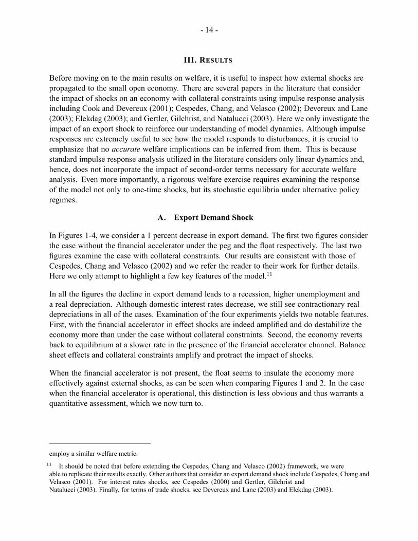
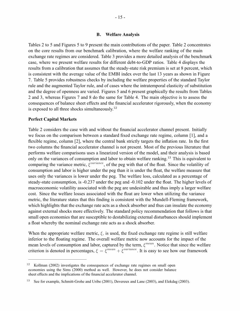
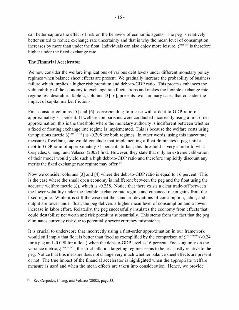
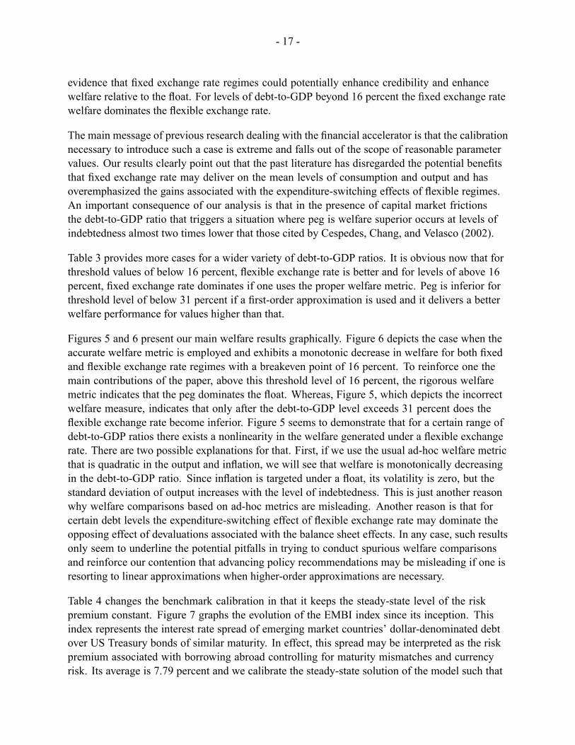
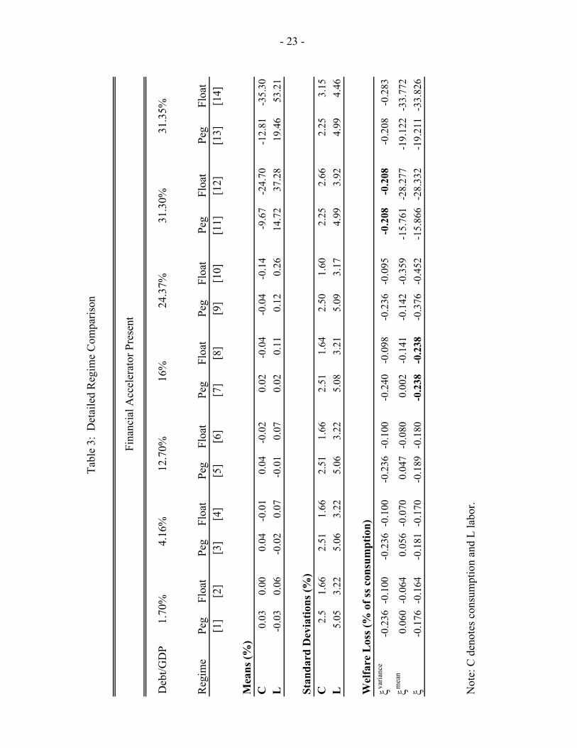
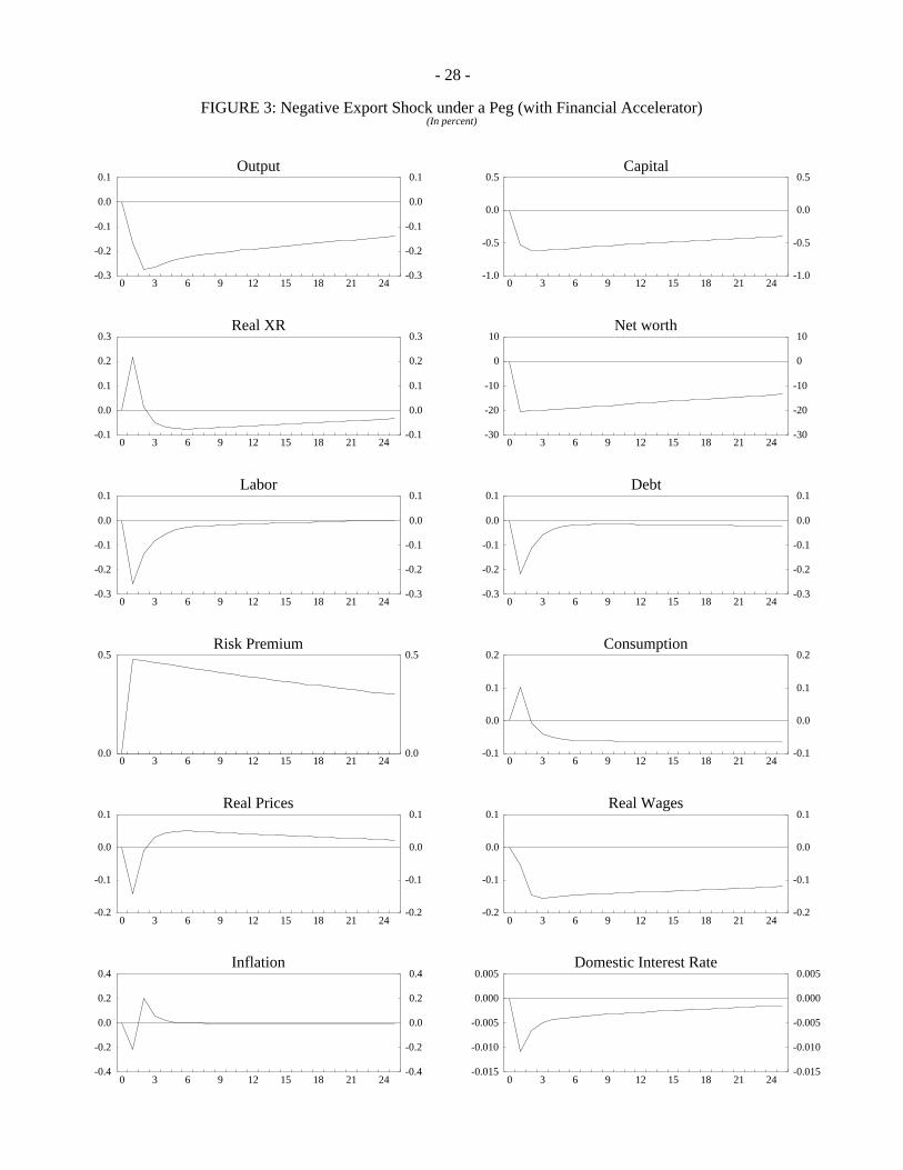
In Figures 1-4, we consider a 1 percent decrease in export demand. The �rst two �gures considerthe case without the �nancial accelerator under the peg and the �oat respectively. The last two�gures examine the case with collateral constraints. Our results are consistent with those ofCespedes, Chang and Velasco (2002) and we refer the reader to their work for further details.Here we only attempt to highlight a few key features of the model.11
In all the �gures the decline in export demand leads to a recession, higher unemployment anda real depreciation. Although domestic interest rates decrease, we still see contractionary realdepreciations in all of the cases. Examination of the four experiments yields two notable features.First, with the �nancial accelerator in effect shocks are indeed ampli�ed and do destabilize theeconomy more than under the case without collateral constraints. Second, the economy revertsback to equilibrium at a slower rate in the presence of the �nancial accelerator channel. Balancesheet effects and collateral constraints amplify and protract the impact of shocks.
When the �nancial accelerator is not present, the �oat seems to insulate the economy moreeffectively against external shocks, as can be seen when comparing Figures 1 and 2. In the casewhen the �nancial accelerator is operational, this distinction is less obvious and thus warrants aquantitative assessment, which we now turn to.
employ a similar welfare metric.11 It should be noted that before extending the Cespedes, Chang and Velasco (2002) framework, we wereable to replicate their results exactly. Other authors that consider an export demand shock include Cespedes, Chang andVelasco (2001). For interest rates shocks, see Cespedes (2000) and Gertler, Gilchrist andNatalucci (2003). Finally, for terms of trade shocks, see Devereux and Lane (2003) and Elekdag (2003).
- 15 -
B. Welfare Analysis
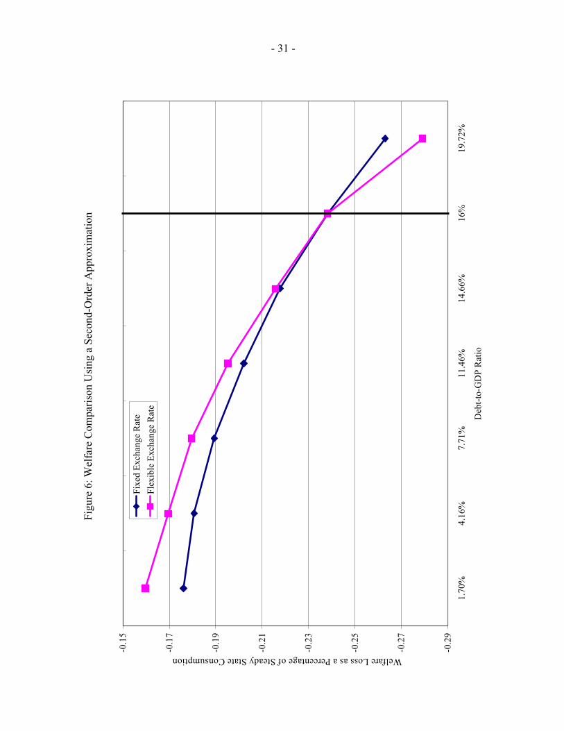
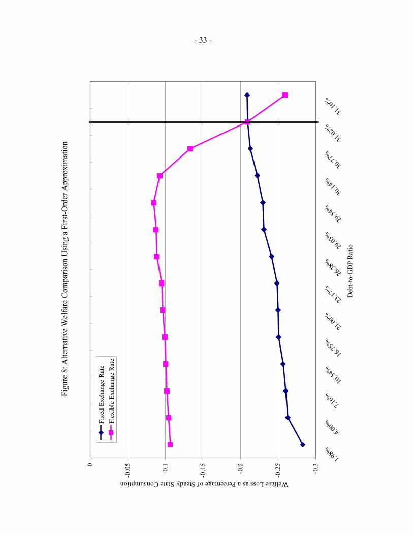
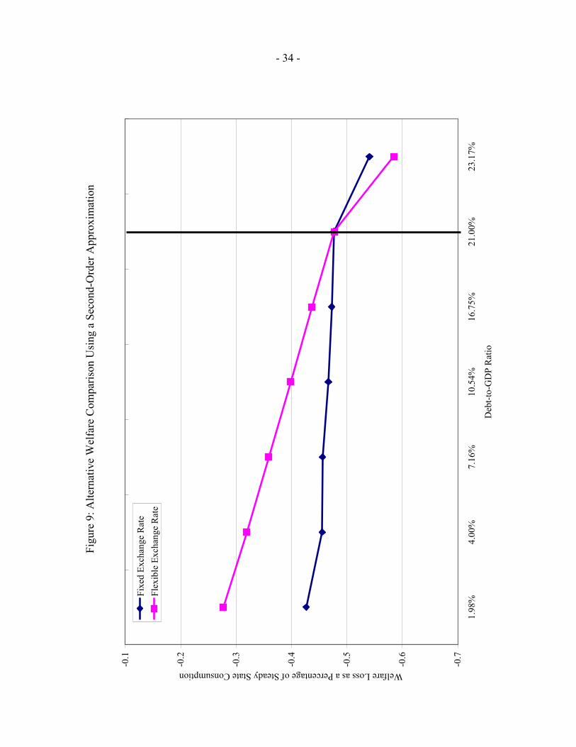
Tables 2 to 5 and Figures 5 to 9 present the main contributions of the paper. Table 2 concentrateson the core results from our benchmark calibration, where the welfare ranking of the mainexchange rate regimes are considered. Table 3 provides a more detailed analysis of the benchmarkcase, where we present welfare results for different debt-to-GDP ratios. Table 4 displays theresults from a calibration that assumes that the steady-state risk premium is set at 8 percent, whichis consistent with the average value of the EMBI index over the last 13 years as shown in Figure7. Table 5 provides robustness checks by including the welfare properties of the standard Taylorrule and the augmented Taylor rule, and of cases where the intratemporal elasticity of substitutionand the degree of openness are varied. Figures 5 and 6 present graphically the results from Tables2 and 3, whereas Figures 7 and 8 do the same for Table 4. The main objective is to assess theconsequences of balance sheet effects and the �nancial accelerator rigorously, when the economyis exposed to all three shocks simultaneously.12
Perfect Capital Markets
Table 2 considers the case with and without the �nancial accelerator channel present. Initiallywe focus on the comparison between a standard �xed exchange rate regime, column [1], and a�exible regime, column [2], where the central bank strictly targets the in�ation rate. In the �rsttwo columns the �nancial accelerator channel is not present. Most of the previous literature thatperforms welfare comparisons uses a linearized version of the model, and their analysis is basedonly on the variances of consumption and labor to obtain welfare ranking.13 This is equivalent tocomparing the variance metric, �variance, of the peg with that of the �oat. Since the volatility ofconsumption and labor is higher under the peg than it is under the �oat, the welfare measure thatuses only the variances is lower under the peg. The welfare loss, calculated as a percentage ofsteady-state consumption, is -0.237 under the peg and -0.102 under the �oat. The higher levels ofmacroeconomic volatility associated with the peg are undesirable and thus imply a larger welfarecost. Since the welfare losses associated with the �oat are lower when utilizing the variancemetric, the literature states that this �nding is consistent with the Mundell-Fleming framework,which highlights that the exchange rate acts as a shock absorber and thus can insulate the economyagainst external shocks more effectively. The standard policy recommendation that follows is thatsmall open economies that are susceptible to destabilizing external disturbances should implementa �oat whereby the nominal exchange rate acts as a shock absorber.
When the appropriate welfare metric, �; is used, the �xed exchange rate regime is still welfareinferior to the �oating regime. The overall welfare metric now accounts for the impact of themean levels of consumption and labor, captured by the term, �mean. Notice that since the welfarecriterion is denoted in percentages, � = �mean + �variance: It is easy to see how our framework
12 Kollman (2002) investigates the consequences of exchange rate regimes on small openeconomies using the Sims (2000) method as well. However, he does not consider balancesheet effects and the implications of the �nancial accelerator channel.13 See for example, Schmitt-Grohe and Uribe (2001), Devereux and Lane (2003), and Elekdag (2003).
- 16 -
can better capture the effect of risk on the behavior of economic agents. The peg is relativelybetter suited to reduce exchange rate uncertainty and that is why the mean level of consumptionincreases by more than under the �oat. Individuals can also enjoy more leisure. �mean is thereforehigher under the �xed exchange rate.
The Financial Accelerator
We now consider the welfare implications of various debt levels under different monetary policyregimes when balance sheet effects are present. We gradually increase the probability of businessfailure which implies a higher risk premium and debt-to-GDP ratio. This process enhances thevulnerability of the economy to exchange rate �uctuations and makes the �exible exchange rateregime less desirable. Table 2, columns [3]-[6], presents two summary cases that consider theimpact of capital market frictions.
First consider columns [5] and [6], corresponding to a case with a debt-to-GDP ratio ofapproximately 31 percent. If welfare comparisons were conducted incorrectly using a �rst-orderapproximation, this is the threshold where the monetary authority is indifferent between whethera �xed or �oating exchange rate regime is implemented. This is because the welfare costs usingthe spurious metric (�variance) is -0.208 for both regimes. In other words, using this inaccuratemeasure of welfare, one would conclude that implementing a �oat dominates a peg until adebt-to-GDP ratio of approximately 31 percent. In fact, this threshold is very similar to whatCespedes, Chang, and Velasco (2002) �nd. However, they state that only an extreme calibrationof their model would yield such a high debt-to-GDP ratio and therefore implicitly discount anymerits the �xed exchange rate regime may offer.14
Now we consider columns [3] and [4] where the debt-to-GDP ratio is equal to 16 percent. Thisis the case where the small open economy is indifferent between the peg and the �oat using theaccurate welfare metric (�), which is -0.238. Notice that there exists a clear trade-off betweenthe lower volatility under the �exible exchange rate regime and enhanced mean gains from the�xed regime. While it is still the case that the standard deviations of consumption, labor, andoutput are lower under �oat, the peg delivers a higher mean level of consumption and a lowerincrease in labor effort. Relatedly, the peg successfully insulates the economy from effects thatcould destabilize net worth and risk premium substantially. This stems from the fact that the pegeliminates currency risk due to potentially severe currency mismatches.
It is crucial to underscore that incorrectly using a �rst-order approximation in our frameworkwould still imply that �oat is better than �xed as exempli�ed by the comparison of �variance(-0.24for a peg and -0.098 for a �oat) when the debt-to-GDP level is 16 percent. Focusing only on thevariance metric, �variance, the strict in�ation targeting regime seems to be less costly relative to thepeg. Notice that this measure does not change very much whether balance sheet effects are presentor not. The true impact of the �nancial accelerator is highlighted when the appropriate welfaremeasure is used and when the mean effects are taken into consideration. Hence, we provide
14 See Cespedes, Chang, and Velasco (2002), page 33.
- 17 -
evidence that �xed exchange rate regimes could potentially enhance credibility and enhancewelfare relative to the �oat. For levels of debt-to-GDP beyond 16 percent the �xed exchange ratewelfare dominates the �exible exchange rate.
The main message of previous research dealing with the �nancial accelerator is that the calibrationnecessary to introduce such a case is extreme and falls out of the scope of reasonable parametervalues. Our results clearly point out that the past literature has disregarded the potential bene�tsthat �xed exchange rate may deliver on the mean levels of consumption and output and hasoveremphasized the gains associated with the expenditure-switching effects of �exible regimes.An important consequence of our analysis is that in the presence of capital market frictionsthe debt-to-GDP ratio that triggers a situation where peg is welfare superior occurs at levels ofindebtedness almost two times lower that those cited by Cespedes, Chang, and Velasco (2002).
Table 3 provides more cases for a wider variety of debt-to-GDP ratios. It is obvious now that forthreshold values of below 16 percent, �exible exchange rate is better and for levels of above 16percent, �xed exchange rate dominates if one uses the proper welfare metric. Peg is inferior forthreshold level of below 31 percent if a �rst-order approximation is used and it delivers a betterwelfare performance for values higher than that.
Figures 5 and 6 present our main welfare results graphically. Figure 6 depicts the case when theaccurate welfare metric is employed and exhibits a monotonic decrease in welfare for both �xedand �exible exchange rate regimes with a breakeven point of 16 percent. To reinforce one themain contributions of the paper, above this threshold level of 16 percent, the rigorous welfaremetric indicates that the peg dominates the �oat. Whereas, Figure 5, which depicts the incorrectwelfare measure, indicates that only after the debt-to-GDP level exceeds 31 percent does the�exible exchange rate become inferior. Figure 5 seems to demonstrate that for a certain range ofdebt-to-GDP ratios there exists a nonlinearity in the welfare generated under a �exible exchangerate. There are two possible explanations for that. First, if we use the usual ad-hoc welfare metricthat is quadratic in the output and in�ation, we will see that welfare is monotonically decreasingin the debt-to-GDP ratio. Since in�ation is targeted under a �oat, its volatility is zero, but thestandard deviation of output increases with the level of indebtedness. This is just another reasonwhy welfare comparisons based on ad-hoc metrics are misleading. Another reason is that forcertain debt levels the expenditure-switching effect of �exible exchange rate may dominate theopposing effect of devaluations associated with the balance sheet effects. In any case, such resultsonly seem to underline the potential pitfalls in trying to conduct spurious welfare comparisonsand reinforce our contention that advancing policy recommendations may be misleading if one isresorting to linear approximations when higher-order approximations are necessary.
Table 4 changes the benchmark calibration in that it keeps the steady-state level of the riskpremium constant. Figure 7 graphs the evolution of the EMBI index since its inception. Thisindex represents the interest rate spread of emerging market countries' dollar-denominated debtover US Treasury bonds of similar maturity. In effect, this spread may be interpreted as the riskpremium associated with borrowing abroad controlling for maturity mismatches and currencyrisk. Its average is 7.79 percent and we calibrate the steady-state solution of the model such that
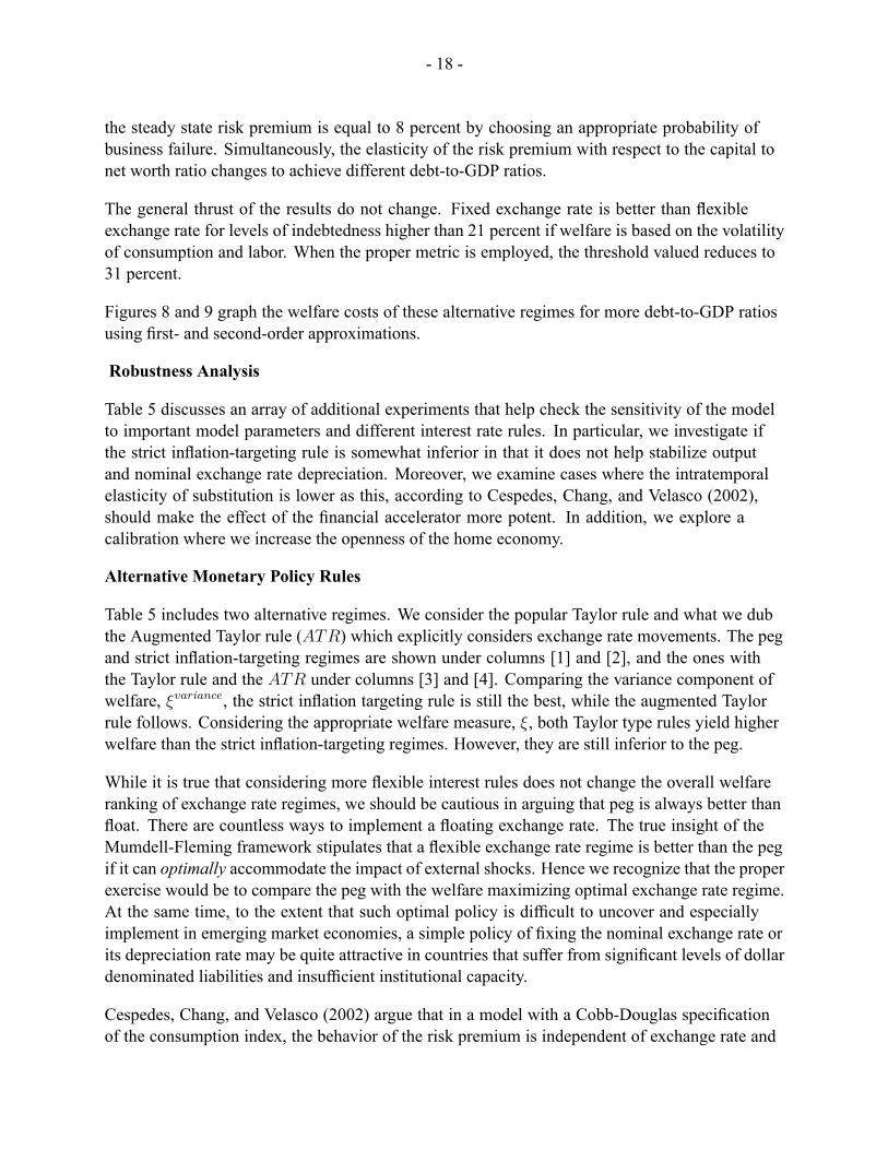
- 18 -
the steady state risk premium is equal to 8 percent by choosing an appropriate probability ofbusiness failure. Simultaneously, the elasticity of the risk premium with respect to the capital tonet worth ratio changes to achieve different debt-to-GDP ratios.
The general thrust of the results do not change. Fixed exchange rate is better than �exibleexchange rate for levels of indebtedness higher than 21 percent if welfare is based on the volatilityof consumption and labor. When the proper metric is employed, the threshold valued reduces to31 percent.
Figures 8 and 9 graph the welfare costs of these alternative regimes for more debt-to-GDP ratiosusing �rst- and second-order approximations.
Robustness Analysis
Table 5 discusses an array of additional experiments that help check the sensitivity of the modelto important model parameters and different interest rate rules. In particular, we investigate ifthe strict in�ation-targeting rule is somewhat inferior in that it does not help stabilize outputand nominal exchange rate depreciation. Moreover, we examine cases where the intratemporalelasticity of substitution is lower as this, according to Cespedes, Chang, and Velasco (2002),should make the effect of the �nancial accelerator more potent. In addition, we explore acalibration where we increase the openness of the home economy.
Alternative Monetary Policy Rules
Table 5 includes two alternative regimes. We consider the popular Taylor rule and what we dubthe Augmented Taylor rule (ATR) which explicitly considers exchange rate movements. The pegand strict in�ation-targeting regimes are shown under columns [1] and [2], and the ones withthe Taylor rule and the ATR under columns [3] and [4]. Comparing the variance component ofwelfare, �variance, the strict in�ation targeting rule is still the best, while the augmented Taylorrule follows. Considering the appropriate welfare measure, �, both Taylor type rules yield higherwelfare than the strict in�ation-targeting regimes. However, they are still inferior to the peg.
While it is true that considering more �exible interest rules does not change the overall welfareranking of exchange rate regimes, we should be cautious in arguing that peg is always better than�oat. There are countless ways to implement a �oating exchange rate. The true insight of theMumdell-Fleming framework stipulates that a �exible exchange rate regime is better than the pegif it can optimally accommodate the impact of external shocks. Hence we recognize that the properexercise would be to compare the peg with the welfare maximizing optimal exchange rate regime.At the same time, to the extent that such optimal policy is dif�cult to uncover and especiallyimplement in emerging market economies, a simple policy of �xing the nominal exchange rate orits depreciation rate may be quite attractive in countries that suffer from signi�cant levels of dollardenominated liabilities and insuf�cient institutional capacity.
Cespedes, Chang, and Velasco (2002) argue that in a model with a Cobb-Douglas speci�cationof the consumption index, the behavior of the risk premium is independent of exchange rate and

- 19 -
monetary regime. However, if the elasticity of substitution between home and foreign goodsis lower than one, a real devaluation increases the risk premium and implies greater �nancialfragility, which might make the peg better than the �oat. We also consider such an extension bypostulating a CES consumption index with an intratemporal elasticity of substitution of � :
C1��t = C1��Ht + (1� )C1��F t (37)
We set � to its lowest possible value of zero and examine the welfare results in columns [5] to[8]. When we use a �rst-order approximation, the breakeven point beyond which peg dominatesdrops to 26 percent. The steady-state risk premium in this case is 6.2 percent and is actuallyis lower than the one when � = 1. Moreover, the welfare loss is bigger with a Cobb-Douglasspeci�cation. Only when we conduct the welfare analysis using a second-order approximation, dowe show that the risk premium relative to the case with � = 1 increases from 1.39 to 3.09 percentand the welfare loss is twice as high as from -0.238 to -0.486 percentage points of steady stateconsumption.
Finally, we increase the openness of the home economy and set = 0:65. Columns [9] to [12]show the results from this exercise. As expected, welfare loss increases substantially for thethreshold values where peg becomes welfare superior to �oat. When =0.75; � =-0.238 andwhen =0.65; � =-1.507.
IV. CONCLUDING REMARKS
We developed a small open-economy model with �nancial frictions and analyzed rigorously thewelfare implications of �xed and �exible exchange rate regimes. We con�rmed that the �exibleexchange rate has better welfare properties than the �xed exchange rate in an economy without�nancial frictions. We found that the presence of a �nancial accelerator mechanism reduceswelfare relative to an economy without �nancial frictions.
Most importantly, we uncovered threshold values of the debt-to-GDP ratios beyond which a pegdominates a �oat. When the model with the �nancial accelerator is solved using linear methodsthis level of indebtedness is around 31 percent. We underlined that the linear-quadratic approachin an environment with sticky prices, monopolistic competition, and imperfect �nancial marketsdelivers spurious and misleading welfare rankings. However, when we utilize a full second-orderexpansion of the model in order to take into account the effect of risk on the behavior of theeconomic agents, we �nd that the threshold is 16 percent. For levels of indebtedness above 16percent, the �xed exchange rate enjoys a credibility advantage and delivers a smaller increase inthe risk premium. This stunts investment to a lesser extent implying milder recessions.
Previous literature has contended that the superiority of the peg over a �oat can be simulated onlyunder extreme calibrations. Moreover, the comparison between exchange rate regimes has beenmostly con�ned to calculating impulse response functions. We have demonstrated that if oneconducts an accurate welfare examination of alternative exchange rate regimes, one does not need

- 20 -
to resort to unreasonable parameter values to come up with a case where peg is welfare superior.In fact, in our view, one can simulate such cases for a wide range of calibrated models.
These results do not, however, imply that �xed exchange rates are universally superior to �exibleexchange rates. It is possible that an optimal monetary policy rule that entails a high degree ofexchange rate �exibility may yield higher welfare than a peg even for debt-to-GDP ratios ofabove 16 percent. In this sense, our analysis should not be viewed as an attempt to change theconventional policy recommendations prescribed by the Mundell-Fleming model.
Our results offer insight on the behavior of authorities in emerging market economies thatface balance sheet effects and provides some theoretical justi�cation for the �Fear of Floating"argument advanced by Calvo and Reinhart (2001). The risk premium associated with borrowingabroad in dollars is a crucial determinant for the choice of an appropriate exchange rate regime.While it could be optimal for such countries to pursue policies implying a �exible exchangerate, such policies may be dif�cult to achieve due to weak institutional infrastructure. From thatperspective, a �xed exchange rate may be more desirable than standard interest rate rules thatallow pronounced nominal exchange rate �exibility.

- 21 -
Table 1. Parameter Calibration
Parameter Value Description� 0.35 Share of K in Y
� 0.99 Subjective discount factor 0.75 Share of CH in C
#i� 0.75 Persistence of i� shock#A 0.9 Persistence of A shock#X 0.5 Persistence of X shockvar("i�) 0.0042 Variance of i� shockvar("A) 0.012 Variance of A shockvar("X) 0.082 Variance of X shock� 10 Substitution elasticity between CHj� 4 Inverse substitution elasticity for C�B 0 Adjustment cost for B�F� 0.0019 Adjustment cost for F �' 200 Adjustment cost for P� 1 Weight of L in utility 1 Inverse substitution elasticity for L

- 22 -
Regime Peg Float Peg Float Peg Float[1] [2] [3] [4] [5] [6]
Means (%)C 0.06 0.01 0.02 -0.04 -9.67 -24.70L -0.05 0.03 0.02 0.11 14.72 37.28Y 0.02 0.06 0.04 0.07 -2.14 -6.27K 0.15 0.11 0.08 0.00 -33.47 -87.14S -0.34 -0.09 -0.23 0.05 21.23 53.96INFL 0.00 0.00 0.00 0.00 -0.01 0.00NW 0.02 -0.02 -2.45 -4.11 -1240.14 -3216.86η 0.00 0.00 0.05 0.08 25.43 67.27D 0.38 0.13 -0.31 -0.03 -35.31 -90.07
Standard Deviations (%)C 2.52 1.68 2.51 1.64 2.25 2.66L 5.05 3.25 5.08 3.21 4.99 3.92Y 3.13 2.29 3.24 2.34 5.75 5.11K 1.36 1.37 1.51 1.49 10.41 15.73S 7.08 4.01 7.08 3.92 7.11 5.17INFL 0.87 0.00 0.91 0.00 1.46 0.00NW 0.96 1.25 19.40 21.34 357.95 568.63η 0.00 0.00 0.35 0.41 7.42 11.86D 8.75 6.53 21.02 21.40 7.57 4.33
Welfare Loss (% of ss consumption)ξvariance -0.237 -0.102 -0.240 -0.098 -0.208 -0.208ξmean 0.097 -0.024 0.002 -0.141 -15.761 -28.277ξ -0.141 -0.125 -0.238 -0.238 -15.866 -28.332
Note: C denotes consumption, L labor, Y output, K capital, S real exchange rate, NW net worth, η the risk premium and D debt.
16%
Financial Accelerator Present
Table 2: Regime Comparison
No Financial Accelerator
31.30%Debt-to-GDP ratio
Reg
ime
Peg
Floa
tPe
gFl
oat
Peg
Floa
tPe
gFl
oat
Peg
Floa
tPe
gFl
oat
Peg
Floa
t[1
][2
][3
][4
][5
][6
][7
][8
][9
][1
0][1
1][1
2][1
3][1
4]
Mea
ns (%
)C
0.03
0.00
0.04
-0.0
10.
04-0
.02
0.02
-0.0
4-0
.04
-0.1
4-9
.67
-24.
70-1
2.81
-35.
30L
-0.0
30.
06-0
.02
0.07
-0.0
10.
070.
020.
110.
120.
2614
.72
37.2
819
.46
53.2
1
Stan
dard
Dev
iatio
ns (%
)C
2.5
1.66
2.51
1.66
2.51
1.66
2.51
1.64
2.50
1.60
2.25
2.66
2.25
3.15
L5.
053.
225.
063.
225.
063.
225.
083.
215.
093.
174.
993.
924.
994.
46
Wel
fare
Los
s (%
of s
s con
sum
ptio
n)ξva
rianc
e-0
.236
-0.1
00-0
.236
-0.1
00-0
.236
-0.1
00-0
.240
-0.0
98-0
.236
-0.0
95-0
.208
-0.2
08-0
.208
-0.2
83
ξmea
n0.
060
-0.0
640.
056
-0.0
700.
047
-0.0
800.
002
-0.1
41-0
.142
-0.3
59-1
5.76
1-2
8.27
7-1
9.12
2-3
3.77
2ξ
-0.1
76-0
.164
-0.1
81-0
.170
-0.1
89-0
.180
-0.2
38-0
.238
-0.3
76-0
.452
-15.
866
-28.
332
-19.
211
-33.
826
Not
e: C
den
otes
con
sum
ptio
n an
d L
labo
r.
Deb
t/GD
P16
%24
.37%
1.70
%4.
16%
12.7
0% Fin
anci
al A
ccel
erat
or P
rese
nt
Tabl
e 3:
Det
aile
d R
egim
e C
ompa
rison
31.3
0%31
.35%
- 23 -

Reg
ime
Peg
Floa
tPe
gFl
oat
Peg
Floa
tPe
gFl
oat
Peg
Floa
tPe
gFl
oat
Peg
Floa
t[1
][2
][3
][4
][5
][6
][7
][8
][9
][1
0][1
1][1
2][1
3][1
4]
Mea
ns (%
)C
-0.0
4-0
.06
-0.0
5-0
.06
-0.0
6-0
.08
-0.0
7-0
.14
-0.3
4-0
.62
-9.4
2-2
4.41
-11.
50-3
1.34
L0.
170.
160.
170.
170.
180.
210.
190.
280.
611.
0214
.37
36.8
617
.51
47.2
9
Stan
dard
Dev
iatio
ns (%
)C
2.62
1.67
2.61
1.66
2.59
1.64
2.55
1.60
2.48
1.52
2.24
2.68
2.24
3.01
L5.
443.
235.
433.
225.
413.
225.
303.
255.
263.
135.
043.
935.
034.
28
Wel
fare
Los
s (%
of s
s con
sum
ptio
n)ξva
rianc
e-0
.283
-0.1
07-0
.263
-0.1
05-0
.260
-0.1
02-0
.250
-0.0
97-0
.242
-0.0
89-0
.210
-0.2
10-0
.209
-0.2
59
ξmea
n-0
.134
-0.1
70-0
.194
-0.2
15-0
.196
-0.2
57-0
.228
-0.3
82-0
.855
-1.4
54-1
5.48
0-2
8.10
3-1
7.79
6-3
1.92
3ξ
-0.4
27-0
.277
-0.4
55-0
.319
-0.4
56-0
.359
-0.4
77-0
.477
-1.0
88-1
.537
-15.
587
-28.
160
-17.
892
-31.
979
Not
e: C
den
otes
con
sum
ptio
n an
d L
labo
r.
Tabl
e 4:
Alte
rnat
ive
Reg
ime
Com
paris
on
Fin
anci
al A
ccel
erat
or P
rese
nt
Deb
t/GD
P1.
98%
4.00
%7.
16%
21.0
0%26
.38%
31.0
2%31
.10%
- 24 -

Reg
ime
Peg
Floa
tTa
ylor
ATR
Peg
Floa
tPe
gFl
oat
Peg
Floa
tPe
gFl
oat
[1]
[2]
[3]
[4]
[5]
[6]
[7]
[8]
[9]
[10]
[11]
[12]
Mea
ns (%
)C
-2.2
4-4
.52
-3.3
0-3
.11
-0.1
2-0
.19
-2.2
9-9
.36
-0.4
4-0
.55
-30.
67-5
0.43
L3.
486.
894.
704.
680.
260.
283.
6214
.02
0.85
0.99
46.6
376
.22
Stan
dard
Dev
iatio
ns (%
)C
2.34
1.59
2.63
2.21
1.83
1.33
1.79
2.13
3.03
1.86
2.42
3.10
L5.
053.
004.
994.
414.
132.
284.
153.
296.
734.
256.
334.
74
Wel
fare
Los
s (%
of s
tead
y st
ate
cons
umpt
ion)
ξvaria
nce
-0.2
19-0
.089
-0.2
45-0
.181
-0.1
41-0
.058
-0.1
38-0
.138
-0.3
76-0
.147
-0.2
89-0
.289
ξmea
n-4
.765
-8.7
16-6
.440
-6.2
85-0
.345
-0.4
29-4
.907
-15.
295
-1.1
46-1
.368
-31.
656
-39.
406
ξ-4
.945
-8.7
78-6
.628
-6.4
25-0
.486
-0.4
86-5
.020
-15.
365
-1.5
07-1
.507
-31.
720
-39.
445
Hom
e ec
onom
y m
ore
open
γ=0.
65
Not
e: C
den
otes
con
sum
ptio
n an
d L
labo
r.
30.9
7%
Less
intra
tem
pora
l ela
stic
ity
Ө
=0
Tabl
e 5:
Com
paris
ons w
ith O
ther
Reg
imes
and
Cal
ibra
tions
Deb
t/GD
P26
.02%
31.1
0%26
.88%
31.3
7%
Fin
anci
al A
ccel
erat
or P
rese
nt
- 25 -

- 26 -
FIGURE 1: Negative Export Shock under a Peg (No Financial Accelerator)(In percent)
-0.2
-0.1
0.0
0.1
-0.2
-0.1
0.0
0.1
0 3 6 9 12 15 18 21 24
Output
-0.04
-0.02
0.00
0.02
-0.04
-0.02
0.00
0.02
0 3 6 9 12 15 18 21 24
Capital
-0.05
0.00
0.05
0.10
0.15
-0.05
0.00
0.05
0.10
0.15
0 3 6 9 12 15 18 21 24
Real XR
-0.10
-0.05
0.00
0.05
-0.10
-0.05
0.00
0.05
0 3 6 9 12 15 18 21 24
Net worth
-0.3
-0.2
-0.1
0.0
0.1
-0.3
-0.2
-0.1
0.0
0.1
0 3 6 9 12 15 18 21 24
Labor
0.0
0.1
0.2
0.3
0.0
0.1
0.2
0.3
0 3 6 9 12 15 18 21 24
Debt
-0.1
0.1
-0.1
0.1
0 3 6 9 12 15 18 21 24
Risk Premium
0.00
0.05
0.10
0.15
0.00
0.05
0.10
0.15
0 3 6 9 12 15 18 21 24
Consumption
-0.10
-0.05
0.00
0.05
-0.10
-0.05
0.00
0.05
0 3 6 9 12 15 18 21 24
Real Prices
0.00
0.01
0.02
0.03
0.04
0.00
0.01
0.02
0.03
0.04
0 3 6 9 12 15 18 21 24
Real Wages
-0.2
-0.1
0.0
0.1
-0.2
-0.1
0.0
0.1
0 3 6 9 12 15 18 21 24
Inflation
-0.006
-0.004
-0.002
0.000
0.002
-0.006
-0.004
-0.002
0.000
0.002
0 3 6 9 12 15 18 21 24
Domestic Interest Rate

- 27 -
FIGURE 2: Negative Export Shock under a Float (No Financial Accelerator)(In percent)
-0.15
-0.10
-0.05
0.00
0.05
-0.15
-0.10
-0.05
0.00
0.05
0 3 6 9 12 15 18 21 24
Output
-0.04
-0.02
0.00
0.02
-0.04
-0.02
0.00
0.02
0 3 6 9 12 15 18 21 24
Capital
-0.1
0.0
0.1
0.2
-0.1
0.0
0.1
0.2
0 3 6 9 12 15 18 21 24
Real XR
-0.10
-0.05
0.00
0.05
-0.10
-0.05
0.00
0.05
0 3 6 9 12 15 18 21 24
Net worth
-0.3
-0.2
-0.1
0.0
0.1
-0.3
-0.2
-0.1
0.0
0.1
0 3 6 9 12 15 18 21 24
Labor
0.0
0.1
0.2
0.3
0.0
0.1
0.2
0.3
0 3 6 9 12 15 18 21 24
Debt
-0.1
0.1
-0.1
0.1
0 3 6 9 12 15 18 21 24
Risk Premium
0.00
0.05
0.10
0.00
0.05
0.10
0 3 6 9 12 15 18 21 24
Consumption
-0.15
-0.10
-0.05
0.00
0.05
-0.15
-0.10
-0.05
0.00
0.05
0 3 6 9 12 15 18 21 24
Real Prices
-0.03
-0.02
-0.01
0.00
0.01
-0.03
-0.02
-0.01
0.00
0.01
0 3 6 9 12 15 18 21 24
Real Wages
-0.1
0.1
-0.1
0.1
0 3 6 9 12 15 18 21 24
Inflation
-0.10
-0.05
0.00
0.05
-0.10
-0.05
0.00
0.05
0 3 6 9 12 15 18 21 24
Domestic Interest Rate
- 28 -
FIGURE 3: Negative Export Shock under a Peg (with Financial Accelerator)(In percent)
-0.3
-0.2
-0.1
0.0
0.1
-0.3
-0.2
-0.1
0.0
0.1
0 3 6 9 12 15 18 21 24
Output
-1.0
-0.5
0.0
0.5
-1.0
-0.5
0.0
0.5
0 3 6 9 12 15 18 21 24
Capital
-0.1
0.0
0.1
0.2
0.3
-0.1
0.0
0.1
0.2
0.3
0 3 6 9 12 15 18 21 24
Real XR
-30
-20
-10
0
10
-30
-20
-10
0
10
0 3 6 9 12 15 18 21 24
Net worth
-0.3
-0.2
-0.1
0.0
0.1
-0.3
-0.2
-0.1
0.0
0.1
0 3 6 9 12 15 18 21 24
Labor
-0.3
-0.2
-0.1
0.0
0.1
-0.3
-0.2
-0.1
0.0
0.1
0 3 6 9 12 15 18 21 24
Debt
0.0
0.5
0.0
0.5
0 3 6 9 12 15 18 21 24
Risk Premium
-0.1
0.0
0.1
0.2
-0.1
0.0
0.1
0.2
0 3 6 9 12 15 18 21 24
Consumption
-0.2
-0.1
0.0
0.1
-0.2
-0.1
0.0
0.1
0 3 6 9 12 15 18 21 24
Real Prices
-0.2
-0.1
0.0
0.1
-0.2
-0.1
0.0
0.1
0 3 6 9 12 15 18 21 24
Real Wages
-0.4
-0.2
0.0
0.2
0.4
-0.4
-0.2
0.0
0.2
0.4
0 3 6 9 12 15 18 21 24
Inflation
-0.015
-0.010
-0.005
0.000
0.005
-0.015
-0.010
-0.005
0.000
0.005
0 3 6 9 12 15 18 21 24
Domestic Interest Rate
- 29 -
FIGURE 4: Negative Export Shock under a Float (with Financial Accelerator)(In percent)
-0.3
-0.2
-0.1
0.0
0.1
-0.3
-0.2
-0.1
0.0
0.1
0 3 6 9 12 15 18 21 24
Output
-1.0
-0.5
0.0
0.5
-1.0
-0.5
0.0
0.5
0 3 6 9 12 15 18 21 24
Capital
-0.2
0.0
0.2
0.4
-0.2
0.0
0.2
0.4
0 3 6 9 12 15 18 21 24
Real XR
-30
-20
-10
0
10
-30
-20
-10
0
10
0 3 6 9 12 15 18 21 24
Net worth
-0.3
-0.2
-0.1
0.0
0.1
-0.3
-0.2
-0.1
0.0
0.1
0 3 6 9 12 15 18 21 24
Labor
-0.4
-0.2
0.0
0.2
-0.4
-0.2
0.0
0.2
0 3 6 9 12 15 18 21 24
Debt
0.0
0.2
0.4
0.6
0.8
0.0
0.2
0.4
0.6
0.8
0 3 6 9 12 15 18 21 24
Risk Premium
-0.15
-0.10
-0.05
0.00
0.05
-0.15
-0.10
-0.05
0.00
0.05
0 3 6 9 12 15 18 21 24
Consumption
-0.3
-0.2
-0.1
0.0
0.1
-0.3
-0.2
-0.1
0.0
0.1
0 3 6 9 12 15 18 21 24
Real Prices
-0.3
-0.2
-0.1
0.0
0.1
-0.3
-0.2
-0.1
0.0
0.1
0 3 6 9 12 15 18 21 24
Real Wages
-0.1
0.1
-0.1
0.1
0 3 6 9 12 15 18 21 24
Inflation
-0.3
-0.2
-0.1
0.0
0.1
-0.3
-0.2
-0.1
0.0
0.1
0 3 6 9 12 15 18 21 24
Domestic Interest Rate

Figu
re 5
: Wel
fare
Com
paris
on U
sing
a F
irst-O
rder
App
roxi
mat
ion
-0.3
-0.2
5
-0.2
-0.1
5
-0.1
-0.0
50
1.70%
4.16%
7.71%
11.46
%
14.66
%
16%
19.72
%
24.37
%
26.38
%
29.03
%
30.48
%
30.97
%
31.11
%
31.25
%
31.30
%
31.35
%
Deb
t-to-
GD
P R
atio
Welfare Loss as a Percentage of Steady State Consumption
Fixe
d Ex
chan
ge R
ate
Flex
ible
Exc
hang
e R
ate
- 30 -
Figu
re 6
: Wel
fare
Com
pari
son
Usi
ng a
Sec
ond-
Ord
er A
ppro
xim
atio
n
-0.2
9
-0.2
7
-0.2
5
-0.2
3
-0.2
1
-0.1
9
-0.1
7
-0.1
5
1.70
%4.
16%
7.71
%11
.46%
14.6
6%16
%19
.72%
Deb
t-to
-GD
P R
atio
Welfare Loss as a Percentage of Steady State Consumption
Fixe
d Ex
chan
ge R
ate
Flex
ible
Exc
hang
e R
ate
- 31 -

Figu
re 7
: Em
ergi
ng M
arke
ts B
onds
Inde
x
024681012141618 Dec-90
Jun-91
Dec-91
Jun-92
Dec-92
Jun-93
Dec-93
Jun-94
Dec-94
Jun-95
Dec-95
Jun-96
Dec-96
Jun-97
Dec-97
Jun-98
Dec-98
Jun-99
Dec-99
Jun-00
Dec-00
Jun-01
Dec-01
Jun-02
Dec-02
Jun-03
Dec-03
EMB
IA
vera
ge
- 32 -
Figu
re 8
: Alte
rnat
ive
Wel
fare
Com
pari
son
Usi
ng a
Fir
st-O
rder
App
roxi
mat
ion
-0.3
-0.2
5
-0.2
-0.1
5
-0.1
-0.0
50
1.98%
4.00%
7.16%
10.54
%
16.75
%
21.00
%
23.17
%
26.38
%
29.03
%
29.54
%
30.14
%
30.77
%
31.02
%
31.10
%
Deb
t-to
-GD
P R
atio
Welfare Loss as a Percentage of Steady State Consumption
Fixe
d Ex
chan
ge R
ate
Flex
ible
Exc
hang
e R
ate
- 33 -
Figu
re 9
: Alte
rnat
ive
Wel
fare
Com
paris
on U
sing
a S
econ
d-O
rder
App
roxi
mat
ion
-0.7
-0.6
-0.5
-0.4
-0.3
-0.2
-0.1
1.98
%4.
00%
7.16
%10
.54%
16.7
5%21
.00%
23.1
7%
Deb
t-to-
GD
P R
atio
Welfare Loss as a Percentage of Steady State Consumption
Fixe
d Ex
chan
ge R
ate
Flex
ible
Exc
hang
e R
ate
- 34 -
- 35 -
References
Bergin, Paul, and Ivan Tchakarov, 2003, “Does Exchange Rate Risk Matter for Welfare? A
Quantitative Investigation,” NBER Working Paper No. 9900 (Cambridge, Massachusetts: National Bureau of Economic Research).
Bernanke, Ben, Mark Gertler, and Simon Gilchrist, 2000, "The Financial Accelerator in a
Quantitative Business Cycle Framework," Handbook of Macroeconomics ( North Holland).
Calvo, Guillermo and Carmen Reinhart, 2001, "Fear of Floating," (unpublished; College Park, Maryland: University of Maryland).
Cespedes, Luis, 2000, "Credit Constraints and Macroeconomic Instability in a Small Open
Economy," (unpublished; New York, New York: New York University). Cespedes, Luis, Roberto Chang, and Andres Velasco, 2001, "Dollarization of Liabilities, Net
Worth Effects, and Optimal Monetary Policy," (unpublished; New York, New York: New York University).
Cespedes, Luis, Roberto Chang, and Andres Velasco, 2002, "Balance Sheet and Exchange
Rate Policy," (unpublished; Cambridge, Massachusetts: Harvard University). Choi, Woon,and David Cook, 2004, "Liability Dollarization and the Bank Balance Sheet
Channel," Journal of Monetary Economics, forthcoming. Collard, Fabrice and Michel Juillard, 2003, "Stochastic Simulations with DYNARE. A
Practical Guide," (unpublished; Toulouse, France: University of Toulouse). Cook, David, and Michael Devereux, 2001, "The Macroeconomics of International Financial
Panics," (unpublished; Vancouver, Canada: University of British Columbia). Devereux, Michael and Philip Lane, 2003, "Exchange Rates and Monetary Policy in
Emerging Market Economies," (unpublished: Dublin, Ireland: Trinity College). Devereux, Michael, 2004, “ Monetary Policy Rules and Exchange Rate Flexibility in a
Simple Dynamic General Equilibrium Model,” (unpublished; Vancouver, Canada: University of British Columbia).
Elekdag, Selim, 2003, "Exchange Rate Regimes and Monetary Policy for Turkey,"
(unpublished: Washington, DC: International Monetary Fund). Eichengreen, Barry, and Ricardo Hausman, 1999, "Exchange Rates and Financial
Fragility," NBER Working Paper No. 7418 (Cambridge, Massachusetts: National Bureau of Economic Research).

- 36 -
Friedman, Milton, 1953, Essays in Positive Economics, (Chicago: University of Chicago
Press). Gertler, Mark, Simon Gilchrist, and Fabio Natalucci, 2003, "External Constraints on
Monetary Policy and the Financial Accelerator," BIS Working Paper No.139 (Basel, Switzerland).
Hunt, Benjamin, Peter Isard, and Douglas Laxton, 2002, "The Role of Exchange Rates in
Inflation Targeting Regimes," (unpublished; Washington, DC: International Monetary Fund).
Juillard, Michel, and Douglas Laxton, 2003, “The IMF`s Global Economy Model: The
Collection of DYNARE Programs Used for Model Solution and Analysis, “ (unpublished; Washington, DC: International Monetary Fund).
Kim, Jinill, and Sunghyan Kim, 2003, "Spurious Welfare Reversals in International Business
Cycle Models,” Journal of International Economics, Vol 60. pp. 471-500. Kollmann, Robert, 2002, “Monetary Policy in the Open Economy: Effects on Welfare and
Business Cycles,” Journal of Monetary Economics, Vol.49, pp. 989–1015. ———, 2003, "Monetary Policy Rules in an Interdependent World,"
(unpublished; Bonn, Germany: University of Bonn). Lane, Philip, and Gian Maria Milesi-Ferretti, 2002, “Long-Term Capital Movement,” NBER
Macroeconomics Annual 2001 (Cambridge, Massachusetts: National Bureau of Economic Research).
Rotemberg, Julio, 1982, "Sticky Prices in the United States," Journal of Political Economy,
vol. 90, pp. 1187-1211. Schmitt-Grohe, Stefanie, and Martin Uribe, 2001, "Stabilization Policy and the Costs of
Dollarization," Journal of Money, Credit and Banking, Vol. 33, pp. 482-509. Sims, C., 2000, “Second-order Accurate Solution of Discrete Time Dynamic Equilibrium
Models,” (unpublished; Princeton, New Jersey: Princeton University). Straub, Roland, and Ivan Tchakarov, 2003, “Non-fundamental Exchange Rate Volatility and
Welfare, “ (unpublished; Florence, Italy: European University Institute; Washington, DC: International Monetary Fund).
Woodford, Micheal, 2001, “Inflation Stabilization and Welfare,” NBER Working Paper No.
9900 (Cambridge, Massachusetts: National Bureau of Economic Research).