balanced polymorphism fuels rapid selection in an invasive
TRANSCRIPT

Portland State University Portland State University
PDXScholar PDXScholar
Environmental Science and Management Faculty Publications and Presentations Environmental Science and Management
8-24-2021
Balanced Polymorphism Fuels Rapid Selection in an Balanced Polymorphism Fuels Rapid Selection in an
Invasive Crab Despite High Gene Flow and Low Invasive Crab Despite High Gene Flow and Low
Genetic Diversity. Genetic Diversity.
C K. Tepolt Woods Hole Oceanographic Institution
E D. Grosholz DepUniversity of California, Davis
Catherine E. de Rivera Portland State University
G M. Ruiz Smithsonian Environmental Research Center, Smithsonian Institution
Follow this and additional works at: https://pdxscholar.library.pdx.edu/esm_fac
Part of the Environmental Sciences Commons
Let us know how access to this document benefits you.
Citation Details Citation Details Tepolt, C. K., Grosholz, E. D., de Rivera, C. E., & Ruiz, G. M. (2021). Balanced polymorphism fuels rapid selection in an invasive crab despite high gene flow and low genetic diversity. Molecular Ecology, mec.16143. https://doi.org/10.1111/mec.16143
This Post-Print is brought to you for free and open access. It has been accepted for inclusion in Environmental Science and Management Faculty Publications and Presentations by an authorized administrator of PDXScholar. Please contact us if we can make this document more accessible: [email protected].

This article has been accepted for publication and undergone full peer review but has not been through the copyediting, typesetting, pagination and proofreading process, which may lead to differences between this version and the Version of Record. Please cite this article as doi: 10.1111/MEC.16143 This article is protected by copyright. All rights reserved
1
2 DR. CAROLYN TEPOLT (Orcid ID : 0000-0002-7062-3452)
3
4
5 Article type : Original Article
6
7
8 Balanced polymorphism fuels rapid selection in an invasive crab9 despite high gene flow and low genetic diversity
10
11 CK Tepolt1,*, ED Grosholz2, CE de Rivera3, GM Ruiz4
12
13 1Department of Biology, Woods Hole Oceanographic Institution, 266 Woods Hole Road,
14 Woods Hole, MA 02543
15 2Department of Environmental Science and Policy, University of California, Davis, CA 95616
16 3Department of Environmental Science and Management, Portland State University, Box 751,
17 Portland, OR 97207
18 4Smithsonian Environmental Research Center, Smithsonian Institution, 647 Contees Wharf
19 Road, Edgewater, MD 21037
20
21 *Corresponding Author:
22 Carolyn Tepolt
23 Department of Biology
24 Woods Hole Oceanographic Institution
25 266 Woods Hole Road, MS #33
26 508-289-3357
28
29
30 Keywords: rapid adaptation, invasive species, island of divergence, seascape genomics, Acc
epte
d A
rtic
le

This article is protected by copyright. All rights reserved
31 balanced polymorphismA
ccep
ted
Art
icle

This article is protected by copyright. All rights reserved
32 Abstract:33
34 Adaptation across environmental gradients has been demonstrated in numerous systems with
35 extensive dispersal, despite high gene flow and consequently low genetic structure. The
36 speed and mechanisms by which such adaptation occurs remain poorly resolved, but are
37 critical to understanding species spread and persistence in a changing world. Here, we
38 investigate these mechanisms in the European green crab Carcinus maenas, a globally
39 distributed invader. We focus on a northwestern Pacific population that spread across >12
40 degrees of latitude in 10 years from a single source, following its introduction <35 years ago.
41 Using six locations spanning >1,500 km, we examine genetic structure using 9,376 Single
42 Nucleotide Polymorphisms (SNPs). We find high connectivity among five locations, with
43 significant structure between these locations and an enclosed lagoon with limited connectivity
44 to the coast. Among the five highly connected locations, the only structure observed was a
45 cline driven by a handful of SNPs strongly associated with latitude and winter temperature.
46 These SNPs are almost exclusively found in a large cluster of genes in strong linkage
47 disequilibrium that was previously identified as a candidate for cold tolerance adaptation in
48 this species. This region may represent a balanced polymorphism that evolved to promote
49 rapid adaptation in variable environments despite high gene flow, and which now contributes
50 to successful invasion and spread in a novel environment. This research suggests an answer
51 to the paradox of genetically depauperate yet successful invaders: populations may be able to
52 adapt via a few variants of large effect despite low overall diversity.
Acc
epte
d A
rtic
le

This article is protected by copyright. All rights reserved
53 Introduction54
55 In the ocean, where many species are characterized by large population sizes, long-distance
56 planktonic dispersal, and broad ranges (Kinlan & Gaines, 2003; Palumbi & Pinsky, 2014),
57 there has been a classical assumption of genetic homogeneity and little persistent
58 differentiation (Hedgecock, 1986). Recently, however, both population genomics and
59 comparative physiology have uncovered evidence of genetic selection and functional
60 differences among widespread populations living across varied marine environments (Sanford
61 & Kelly, 2011; Pespeni & Palumbi, 2013). Likewise, genetic studies and associated modeling
62 have detected subtle genetic structure driven by oceanography in species that disperse
63 widely (Galindo, Olson, & Palumbi, 2006; White et al., 2010; Xuereb et al., 2018). This
64 increasing evidence for differentiation in the sea begs the question of how quickly, and
65 through which mechanisms, marine species may cope with rapidly changing environmental
66 conditions (Munday, Warner, Monro, Pandolfi, & Marshall, 2013). Introduced species, which
67 in many cases establish and thrive in novel habitats, offer the opportunity to examine these
68 questions in the context of the natural environment (Blackburn, 2008; Lee, Kiergaard,
69 Gelembiuk, Eads, & Posavi, 2011).
70
71 Marine species exhibit a spectrum of evolutionary mechanisms based in part on their
72 dispersal. Local adaptation in the classical sense is restricted to species with relatively limited
73 dispersal, which facilitates the selection and retention of adaptive alleles within a population
74 (Kawecki & Ebert, 2004). Relatively isolated populations are also likely to diverge due to
75 neutral processes, as genetic drift changes allele frequencies across the genome (Ellingson &
76 Krug, 2016; Prunier, Dubut, Chikhi, & Blanchet, 2017). On the other end of this evolutionary
77 spectrum lie open marine systems, where alleles are continually exported from each location
78 to a mixed pool of larvae that may settle in environments far different from their sources. In
79 this dynamic, balanced polymorphism is favored, and adaptive variation is maintained within
80 the population as a whole (Sanford & Kelly, 2011). These adaptive alleles mix as larvae
81 disperse, and the environmental conditions they encounter as they recruit can result in strong
82 and rapid selection that culls less-fit alleles from the local population (Sotka, 2012). This
83 phenomenon has been described largely in the context of maintaining differentiation across Acc
epte
d A
rtic
le
This article is protected by copyright. All rights reserved
84 small-scale environmental differences year after year in systems where the scale of dispersal
85 far exceeds the scale of selection. For example, strong selection to salinity appears to have
86 maintained an enzymatic cline in mussels along Long Island Sound (Koehn, Newell, &
87 Immermann, 1980), and microhabitat differences across tidal heights maintain balanced
88 polymorphism in limpet populations (Schmidt, Bertness, & Rand, 2000). Such examples may
89 better reflect the realized capacity of highly dispersive marine species to adapt to stressors
90 across complex oceanographic regimes than studies of strict local adaptation (Véliz,
91 Duchesne, Bourget, & Bernatchez, 2006).
92
93 As species expand into new environments, the process of adaptation may be mediated by the
94 complex demographic effects that often occur at range edges (Bridle & Vines, 2007; Chuang
95 & Peterson, 2016). Expanding populations are frequently characterized by sequential
96 bottlenecks and losses of genetic diversity caused by small groups of colonizing organisms
97 (Eckert, Samis, & Lougheed, 2008; White, Perkins, Heckel, & Searle, 2013; Bors, Herrera,
98 Morris, & Shank, 2019). The success of some such populations, which multiply and spread
99 despite low genetic diversity, has been coined the “genetic paradox of invasions” (Roman &
100 Darling, 2007). These bottlenecks can also lead to increased stochasticity at range edges,
101 causing allele surfing and other distinctive genetic patterns (Excoffier & Ray, 2008). Gene
102 flow plays a substantial role in this process. In some cases, low-diversity edge populations
103 may be evolutionarily limited by a lack of gene flow (Sexton, Strauss, & Rice, 2011;
104 Takahashi et al., 2016), while in others, semi-isolation at range edges permits rapid evolution
105 in organisms at the expansion front (Phillips, Brown, Webb, & Shine, 2006; Kilkenny &
106 Galloway, 2012; Szücs et al., 2017). High dispersal and large populations may also facilitate
107 species persistence and expansion, if functional diversity can be maintained and quickly
108 spread throughout the expanding range (Rius & Darling, 2014). The maintenance of such
109 diversity can in theory provide the raw substrate for adaptation and permit extremely quick
110 evolutionary response to shifting conditions (Tigano & Friesen, 2016; Llaurens, Whibley, &
111 Joron, 2017). However, to date, the relative contributions of selection and drift as populations
112 establish in novel environments have not been explored empirically in high gene flow
113 systems.
114 Acc
epte
d A
rtic
le

This article is protected by copyright. All rights reserved
115 The European green crab (Carcinus maenas) along the northeast Pacific coastline presents
116 an ideal test case for untangling the dynamics of rapid marine adaptation and differentiation
117 with high potential gene flow. In this region, the species established an initial population in
118 San Francisco Bay by 1990 (Carlton & Cohen, 2003), and spread >1,500 km to Vancouver
119 Island in <10 years despite deriving from a single, significantly bottlenecked source (Tepolt et
120 al., 2009). Green crabs advanced along the coast and primarily to the north, reaching
121 northern California by 1995, southern Oregon by 1997, and Vancouver Island, British
122 Columbia by 1998 (Behrens Yamada & Gillespie, 2008; Fig. 1). This rapid expansion was
123 associated with extremely strong positive El Niño-Southern Oscillation (ENSO) indices in
124 1997-1998 that promoted high reproductive output, northward transport, and coastal retention
125 of larvae (Behrens Yamada et al., 2005; Behrens Yamada & Kosro, 2010; See & Feist, 2010).
126 Importantly, in the northeast Pacific, C. maenas are found almost exclusively in shallow
127 waters of protected embayments and not along the exposed outer coast between bays,
128 resulting in a disjunct distribution of green crab populations. This habitat distribution is similar
129 to its introduced range in South Africa, where the rocky coast is also subject to high-energy
130 wave action (Hampton & Griffiths, 2007), but differs from its more continuous distribution in
131 other global regions (Carlton & Cohen, 2003). The species also has a relatively wide
132 environmental tolerance and diet breadth, along with a 30-75 day pelagic larval duration
133 (Dawirs, 1985), which have contributed to its spread and establishment in six introduced
134 regions across five continents (Carlton & Cohen, 2003; Hidalgo, Barón, & Orensanz, 2005).
135
136 The importance of ENSO events in the spread and abundance of northeast Pacific C. maenas
137 suggests that both temperature and local oceanography may play substantial roles in
138 structuring the population. Decades of field surveys of abundance in both the northwest
139 Atlantic and northeast Pacific support the importance of temperature during early
140 development in driving recruitment strength: cold winters have been associated with weaker
141 recruitment and smaller cohorts of crabs than milder years (Behrens Yamada & Kosro, 2010;
142 Welch, 1968). A global physiological study demonstrated population-level differences in adult
143 heat and cold tolerance consistent with local adaptation (Tepolt & Somero, 2014).
144 Subsequently, transcriptomic work has identified genetic markers associated with
145 temperature tolerance on a population level (Tepolt & Palumbi, 2020). Like many marine Acc
epte
d A
rtic
le
This article is protected by copyright. All rights reserved
146 species, C. maenas larvae have shown narrower temperature tolerances than adults in
147 laboratory trials, suggesting that thermal tolerance at early life stages may be particularly
148 important in shaping crab populations across different years (Dawirs, 1985; de Rivera et al.,
149 2007).
150
151 Here, we use transcriptome-derived SNPs from C. maenas populations in the northeast
152 Pacific to test the roles of connectivity and selection in shaping the population structure of this
153 highly dispersive and recently introduced species. Using six sites spanning over 1,500 km of
154 coastline, we examine population structure and relative migration to elucidate connectivity
155 among embayments across the species’ northeast Pacific range. For a few sites, we have
156 temporal samples spanning 2-5 years, which we use to examine the stability of population
157 structure over time. Finally, we test for candidate genes for selection across a thermal
158 latitudinal gradient, comparing these candidates to genes identified in a prior global study of
159 the genetic basis of thermal tolerance differences in the species. As this population was
160 founded <35 years ago from a single source, our data represent patterns of divergence and
161 selection that have arisen in under 20 generations.
162
163 Materials and Methods164
165 Sample Collection
166 Twelve crabs were sampled from each of six sites along the northeast Pacific range of C.
167 maenas in 2015-2016 (Figure 1). Two of these sites (Seadrift Lagoon and San Francisco Bay,
168 CA, USA) were sampled in both years, while the remaining sites were sampled once. We also
169 reanalyzed raw sequence data from a prior study of crabs collected in 2011 from two sites
170 (Seadrift Lagoon, CA, USA and Barkley Sound, BC, Canada; Tepolt & Palumbi 2015). Crabs
171 were collected by hand or trap, and hearts were dissected and stored in RNALater at -80°C.
172
173 Extraction & Sequencing
174 Total RNA was extracted from cardiac tissue using TRIzol (Invitrogen, Carlsbad, CA, USA)
175 with 1-bromo-3-chloropropane (Simms, Cizdziel, & Chomczynski, 1993). RNA was quantified
176 using the broad-range RNA assay on a Qubit 3.0 fluorometer (Invitrogen), and up to 4 μg of Acc
epte
d A
rtic
le

This article is protected by copyright. All rights reserved
177 RNA was used to prepare individually-barcoded cDNA libraries with Ilumina's TruSeq
178 Stranded mRNA Library Prep Kit (Illumina, San Diego, CA, USA). Libraries were sent to the
179 University of California Berkeley’s Genomics Sequencing Laboratory, where they were
180 quantified and pooled into groups of 16 multiplexed samples run on five lanes of an Illumina
181 HiSeq 4000 in 50-bp single-end reads.
182
183 Sequence Processing and SNP Identification
184 Raw sequences were cleaned and trimmed using Trim Galore! v0.6.4
185 (http://www.bioinformatics.babraham.ac.uk/projects/trim_galore/), a wrapper for Cutadapt v2.6
186 (Martin 2011). A nucleotide call quality cutoff of Phred ≥20 was used, and reads ≤20bp after
187 adapter removal and quality trimming were discarded. A published C. maenas cardiac
188 transcriptome was used as a reference (Tepolt & Palumbi 2015), after an expression-based
189 screening to remove poorly-supported contigs and reduce computational load. Briefly, we
190 mapped trimmed and clipped reads from Tepolt & Palumbi 2015 back to the reference
191 transcriptome using salmon v1.2.1 (Patro, Duggal, Love, Irizarry, & Kingsford, 2017). We
192 retained only contigs with TPM >1, and re-annotated these contigs using EnTAP v 0.9.1 (Hart
193 et al. 2020), comparing all 6 reading frames against the Swissprot, TrEMBL, and nr protein
194 databases (downloaded March 2020). Annotations to Decapoda were prioritized with the
195 program’s ‘--taxon’ flag. Contigs with a clear taxonomic mismatch to decapods (e.g., bacteria,
196 green plants, fungi, etc.), as well as all likely mitochondrial and ribosomal contigs, were
197 identified and removed from the project after alignment to minimize non-target mapping. This
198 resulted in a clean reference transcriptome of 25,552 nuclear contigs.
199
200 Cleaned reads were mapped back to the C. maenas cardiac transcriptome using Bowtie2
201 v2.4.1 with default settings (Langmead & Salzberg 2013). Picard v2.22.0 was used to sort
202 reads, identify and mark duplicate read sequences, and index the resulting bam files
203 (http://broadinstitute.github.io/picard). The Genome Analysis Toolkit (GATK) v4.1.7.0 was
204 used to identify and genotype biallelic SNPs (McKenna et al. 2010; DePristo et al. 2011).
205
206 Across all 120 samples (24 from 2011 and 96 from 2015-2016), GATK identified 163,261
207 biallelic SNPs with Phred quality scores ≥20. We identified high-quality, well-supported SNPs Acc
epte
d A
rtic
le

This article is protected by copyright. All rights reserved
208 for downstream analyses using a custom python script that retained only individual genotypes
209 with Phred ≥20 and supported by ≥5 reads. We excluded SNPs missing high-quality
210 genotypes at ≥4 individuals for any site-by-year samples of 12 individuals, SNPs with
211 heterozygosity ≥0.7 (to screen out obvious paralogs), and SNPs where the alternate allele
212 was observed only once across all individuals (to minimize bias by potential sequencing
213 errors). In total, 9,376 SNPs had high-quality genotypes for ≥8 individuals per group and were
214 retained for downstream processing. All 120 individuals had high-quality genotypes at >80%
215 of these SNPs.
216
217 Identification of Putative Inversion Polymorphisms
218 We explored the relationship of the 9,376 high-quality SNPs to identify potential inversion
219 polymorphisms and other disproportionately large groups of SNPs in linkage disequilibirum
220 (LD). Pairwise R2 was calculated across all SNPs using the --geno-r2 and --interchrom-geno-
221 r2 options in vcftools v0.1.16 (Danecek et al. 2011). We then used the R package LDna v0.64
222 to identify networks of SNPs in large, compact clusters, setting minimum edges to 45
223 (expected for 10 closely-linked SNPs) and phi to 15 (Kemppainen et al. 2015).
224
225 We identified one large outlier LD cluster, which contained 168 SNPs from 56 different
226 contigs. To further investigate this cluster, we explored the relationship between member
227 SNPs using Principal Components Analysis (PCA) in smartPCA, implemented in Eigensoft
228 v7.2.1 (Price et al., 2006). We used the 116 individuals that had <20% missing genotypes
229 across the 168 SNPs in this cluster. This PCA separated individuals into three clear groups
230 along PC1, and we calculated FIS within each of these groups to determine relative
231 heterozygosity (Kemppainen et al. 2015). These analyses strongly suggested an inversion
232 polymorphism (see Results below), so for clarity we refer to this group of 168 SNPs as an
233 “inferred inversion” throughout the rest of the manuscript. To compare the impact this putative
234 inversion had on overall population structure, we also ran a PCA on the same 116 individuals
235 using the full SNP set both with and without the 168 SNPs in the inferred inversion (N = 9,376
236 and 9,208 SNPs, respectively).
237
238 Genetic Structure and DiversityAcc
epte
d A
rtic
le
This article is protected by copyright. All rights reserved
239 SNPs were separately screened to identify all sets of markers in linkage disequilibrium (LD)
240 and generate a set of independent SNPs for population genomics. Pairwise R2 values
241 (calculated above) were used to identify groups of two or more SNPs in LD at R2 ≥0.8 using
242 the R package igraph v1.2.4.2 (Csardi & Nepusz 2006), and then all but one SNP in each
243 group was removed, leaving a set of 6,848 independent SNPs. The one SNP retained from
244 each group had the highest number of high-quality genotypes, with lower-coverage SNPs
245 within an LD group preferentially removed. We use the term “independent” to indicate that
246 these SNPs have been screened to remove those in strong LD, but note that these SNPs
247 may be in LD at lower levels so are not all truly independent. Similarly, this set of 6,848
248 independent SNPs retained 54 of the 168 SNPs in the inferred inversion which were in lower
249 levels of LD with each other (R2: 0.29-0.79).
250
251 Basic descriptive statistics were calculated for each site-by-year sample using the set of
252 6,848 independent SNPs (Table 1). Allelic richness (Ar) and private allelic richness (pAr) were
253 determined using ADZE v1.0 (Szpiech, Jakobsson, & Rosenberg, 2008). The R package
254 genepop v1.1.7 was used to calculate observed and expected heterozygosity (Ho and He),
255 and to calculate the inbreeding coefficient (FIS) and test for heterozygote excess or deficiency
256 using Hardy-Weinberg tests (Rousset 2008). The number of polymorphic SNPs in each
257 sample was determined using Arlequin v.3.5.2.2 (linux core implementation; Excoffier &
258 Lischer 2010).
259
260 To identify a subset of putatively neutral SNPs with which to examine population structure
261 unconfounded by selection, we used BayPass v2.2 in the core model (Gautier et al. 2015),
262 with each site-by-year sample treated as its own group. We assessed potential outliers using
263 a simulated pseudo-observed data set of 6,848 SNPs with the parameters of the real data to
264 set a 10% false discovery rate (FDR) threshold for SNP XtX. This conservative threshold was
265 chosen to avoid retaining SNPs under weak selection, thus yielding a set of SNPs more likely
266 to be truly neutral. This frequency-based approach removed all but one of the SNPs later
267 identified as a candidate for environmental association (see below).
268
269 Genetic structure for both the independent (N = 6,848) and putatively neutral (N = 6,311) SNP Acc
epte
d A
rtic
le

This article is protected by copyright. All rights reserved
270 sets was assessed with smartPCA. Pairwise FST was calculated between all site-by-year
271 groups according to Weir & Cockerham's (1984) approach using the R package ‘StAMPP’
272 v1.6.1 with both the independent and putatively neutral SNP sets (Pembleton, Cogan, &
273 Forster, 2013). Significance was assessed using 10,000 permutations, and resulting p-values
274 were adjusted for multiple tests using a Benjamini-Hochberg false discovery rate correction
275 (Benjamini & Hochberg 1995).
276
277 We included only the most recent temporal sample from each site for an analysis of relative
278 migration using the putatively neutral SNP set (Table 1). Symmetry and relative magnitude of
279 migration between sites was assessed using the ‘divMigrate’ function in the R package
280 ‘diveRsity’ v1.9.90, with the Nm method and 1,000 bootstraps (Sundqvist, Keenan,
281 Zackrisson, Prodöhl, & Kleinhans, 2016). This approach, which calculates relative directional
282 migration, was chosen because it is more robust if populations do not perfectly satisfy some
283 of the assumptions underlying approaches to quantify an effective migration rate (e.g., island
284 model, mutation-drift equilibrium).
285
286 All analyses showed strong separation of a single site, Seadrift Lagoon, from all other sites
287 (see Results below). Because of this genetic distinctiveness, isolation-by-distance (IBD)
288 analysis excluded pairwise comparisons with Seadrift Lagoon, focusing only on the remaining
289 five “open” sites. Pairwise FST values were used to plot IBD between sites, using along-shore
290 distance calculated at 50km resolution with the USA map from GADM supplemented with
291 Google Maps for distances <50km (gadm.org). When comparisons spanned San Francisco
292 Bay and the Strait of Juan de Fuca, distances were calculated across the mouths of these
293 features. IBD was plotted using five different SNP sets, to explore different potential drivers of
294 latitudinal structure along the coast: 1) 6,848 independent SNPs, 2) 6,311 putatively neutral
295 SNPs, 3) 54 “independent” SNPs in the inferred inversion, 4) 6,794 independent SNPs
296 excluding the 54 independent SNPs in the inferred inversion 5) 144 outlier SNPs identified
297 among the five “open” sites with BayPass (see Results). The significance of these
298 relationships was assessed using linear regression in R.
299
300 Markers under SelectionAcc
epte
d A
rtic
le

This article is protected by copyright. All rights reserved
301 We identified SNPs potentially under environmental selection using BayPass and
302 Redundancy Analysis (RDA). We ran these tests using only the five open sites, excluding
303 Seadrift Lagoon, to identify markers potentially driving the observed signal of IBD and
304 latitudinal structuring along the coast. For this testing we used a single sample, collected in
305 2015-2016, from each site: 6,662 SNPs of the full 6,848 SNP set were polymorphic in these
306 five samples and were used for tests of selection. Tested covariates included site latitude (as
307 Cartesian Y-values) and winter and summer sea surface temperature (SST). Temperature
308 data were derived from NOAA’s OI SST V2 High Resolution Dataset provided by the
309 NOAA/OAR/ESRL PSD, Boulder, Colorado, USA, from their website at
310 https://www.esrl.noaa.gov/psd/ (Reynolds et al. 2007). Daily temperatures were averaged
311 over the 2 years prior to sampling, and were determined for the nearest 0.25° grid location to
312 each study site for January (winter) and July (summer).
313
314 In BayPass, we first ran a core model analysis to identify frequency outlier SNPs, then used
315 the auxiliary covariate model to test for associations between allele frequencies and latitude
316 and winter and summer SST (Gautier 2015). Covariates were scaled, and we used an Ising
317 prior of 0 since the physical order of contigs is unknown. We considered any SNP with Bayes
318 factor (BF) ≥15 dB to be a candidate for selection with respect to a given covariate.
319
320 We ran an RDA on individual genotypes using the R package ‘vegan’ v2.5-6 (Oksanen et al.
321 2019), with missing genotypes imputed to be the most common observed. Few individual
322 genotypes were missing in our data set: genotyping was ≥90% complete for 97.1% of SNPs,
323 and no single sampling site was missing >4 individual genotypes at any SNP. We used
324 latitude and summer temperature as covariates (RDA formula = individual genotypes ~ Y +
325 July SST); winter temperature was excluded as it was strongly correlated with latitude (R2 =
326 0.79; p = 0.03). We considered any SNP >3 SD outside the mean loading for its RDA axis to
327 be a candidate for selection (e.g., Forester et al., 2018).
328
329 SNPs were considered strong candidates for selection if they were identified by both BayPass
330 and RDA. Latitude is largely correlated with SST in this data set, due both to the strongly
331 linear north-south arrangement of sites along the coast and to the relative coarseness of the Acc
epte
d A
rtic
le
This article is protected by copyright. All rights reserved
332 satellite-derived temperature data. Because of this confounding, we treated all SNPs
333 identified as candidates for association with either latitude or temperature interchangeably. To
334 visualize these relationships, candidate SNPs were tested for linear correlation between
335 minor allele frequency and latitude or temperature.
336
337 Potential Function of Candidate SNPs
338 Candidate SNPs were examined for their potential impact on protein structure, to provide an
339 initial idea of SNPs that were particularly likely to affect organismal function. Open Reading
340 Frames (ORFs) and corresponding coding sequences for all contigs were predicted using
341 OrfPredictor v3.0 (Min, Butler, Storms, & Tsang, 2005); as many contigs could not be
342 annotated, sequence data alone was used to predict ORFs. Predicted sequences were then
343 used to class the impact of a given SNP on the resulting protein sequence (untranslated,
344 synonymous, or non-synonymous) using a custom python script. Of the 9,376 high-quality
345 SNPs, we predicted that 4,339 were in the untranslated regions of the mRNA and two were in
346 contigs for which an ORF could not be predicted. Of the putatively coding SNPs, 3,843 were
347 predicted to be synonymous and 1,192 to be non-synonymous. We examined SNP
348 substitution patterns for all 9,376 candidate SNPs prior to LD screening. While putatively
349 linked SNPs were removed from the data set prior to selection analysis, they could potentially
350 be driving any relationships we detected in SNPs with which they are in strong LD.
351
352 Data manipulation and plotting were done using the data.table and ggplot2 packages in R
353 (Wickham 2009; R Core Team 2016; Dowle & Srinivasan 2017).
354
355 Results356
357 Inferred Inversion Polymorphism
358 Linkage disequilibrium network analysis identified one single outlier LD cluster nested in one
359 compound outlier LD cluster (Figure 2A-B). The compound outlier LD cluster, which we refer
360 to as an “inferred inversion”, contained 168 SNPs at an LD of R2 ≥0.29. PCA of these 168
361 SNPs split individuals into three discrete groups along the first principal component,
362 explaining 73.08% of variance (p = 0.001; Figure 2C). While individuals from most sites Acc
epte
d A
rtic
le
This article is protected by copyright. All rights reserved
363 appeared in all three groups, the left-most group contained predominantly British Columbia
364 and Seadrift Lagoon while the right-most group contained predominantly Elkhorn Slough and
365 San Francisco Bay. This pattern of three distinct groups explaining the majority of structure,
366 with no discrete partitioning of sites, is diagnostic of a region of the genome where
367 recombination is reduced (Kemppainen et al. 2015). In that case, each group represents a
368 karyotype: homozygotes on the left and right sides of PC1, and heterozygotes midway
369 between. Analysis of FIS within each of these groups supports this conclusion, with values
370 near zero in the putative homozygotes (indicating Hardy-Weinberg equilibrium) and strongly
371 negative in the putative heterozygotes (indicating an excess of heterozygous individuals;
372 Figure 2D). Overall FIS is lower in the middle than in the left or right groups (p < 0.0001 for
373 both comparisons), while the left and right groups are not significantly different from each
374 other (p = 0.1).
375
376 Genetic structure over all SNPs showed a significant divide between Seadrift Lagoon and the
377 other five sites, both with and without the 168 SNPs in the inferred inversion (p < 0.0001;
378 Figure 2E-F). With the full set of 9,376 SNPs, individuals in both Seadrift Lagoon and the
379 remaining five “open” sites were further subdivided into three clusters according to their
380 inferred inversion genotype (p < 0.0001; Figure 2C,E). When the 168 SNPs in the inferred
381 inversion were removed, this three-part structure disappeared and the second principal
382 component was no longer significant (p = 0.09; Figure 2F).
383
384 SNP Selection and Genetic Diversity
385 Of the full 9,376 high-quality SNP set, 3,962 SNPs comprised 1,434 groups in LD with R2 ≥
386 0.8; all but one SNP was removed from each group to create a set of 6,848 “independent”
387 SNPs. This screening differs from the earlier LDna analysis, which sought to identify large
388 clusters of LD; by contrast, this approach intends simply to remove bias to population
389 structure measurements from including any sets of SNPs in strong LD. The majority of these
390 groups (N = 839) comprised small numbers of SNPs in the same contig. The largest of these
391 groups by far included 77 SNPs from the inferred inversion; no other groups contained >13
392 SNPs. We note that this analysis did not identify all 168 SNPs in the inferred inversion as
393 being in the same group, since some of those SNPs are in LD with others at R2 < 0.8; Acc
epte
d A
rtic
le

This article is protected by copyright. All rights reserved
394 consequently, the set of 6,848 independent SNPs includes 54 SNPs in the inferred inversion.
395
396 After removing SNPs in strong LD, we had a final working panel of 6,848 high-quality,
397 independent SNPs. BayPass identified 537 of these SNPs as potentially under selection at
398 FDR ≤0.1 across all site-by-year samples; these SNPs were removed to construct a panel of
399 6,311 putatively neutral SNPs for selected downstream analyses.
400
401 Allelic richness ranged from 1.669-1.711 (Table 1); it was significantly lower in Seadrift
402 Lagoon than in all other sites in all years (p ≤ 0.005; Table 1). Private allelic richness was low,
403 ranging from 0.00438-0.00771; seven pairwise comparisons were significant, all comparing
404 Seadrift Lagoon in 2011 or 2016 with non-Seadrift Lagoon sites (p < 0.05 for all
405 comparisons). Lower allelic richness in Seadrift Lagoon reflects a lower number of
406 polymorphic SNPs there than in all other sites (Table 1). All samples showed a significant
407 heterozygote excess.
408
409 Population Structure and Migration
410 FST was significant between most sample pairs when using the 6,848 independent SNP set
411 (pairwise FST excluding temporal comparisons: 0.00058-0.027; SI Table S1). By contrast,
412 when using the 6,311 putatively neutral SNPs nearly all significant comparisons were
413 between Seadrift Lagoon samples and all other sites (pairwise FST including Seadrift: 0.0081-
414 0.016; pairwise FST excluding Seadrift: -0.0021-0.0044; SI Table S2). There was no evidence
415 for differentiation within any temporal comparison across years with the putatively neutral
416 SNP set (pairwise FST: -0.0020-0.0014; SI Table S2). Principal components analysis
417 reinforced these patterns, with the first component separating Seadrift Lagoon from all other
418 sites with both the independent and neutral SNP sets (6,848 independent SNPs: loading =
419 2.75%, p < 0.0001; 6,311 neutral SNPs: loading = 2.07%, p < 0.0001; Figure 3A,B). The
420 second component was significant only with the independent SNP set (loading = 1.53%, p <
421 0.0001), and spread non-Seadrift Lagoon sites along a rough north-south axis (Figure 3A).
422 With the neutral SNP set, this pattern collapsed (p > 0.05), with near-complete overlap among
423 all non-Seadrift Lagoon samples (Figure 3B). While Seadrift Lagoon had significantly lower
424 allelic richness than all other sites, there were no significant differences among the remaining Acc
epte
d A
rtic
le
This article is protected by copyright. All rights reserved
425 open sites (Figure 3C).
426
427 To test a realistic migration scenario, we estimated relative migration using only the most
428 recent sample from each site. Estimates of relative migration between sites (using 6,311
429 neutral SNPs only) demonstrated similar and symmetrical migration among all sites except
430 Seadrift Lagoon (Figure 3D). Consistent with Seadrift Lagoon’s distinctiveness, we found
431 evidence for reduced migration both into and out of this site relative to the rest of our study
432 sites (Figure 3D). The approach we used sets the maximum observed migration to 1 and
433 scales the rest of the migration estimates accordingly. Between all five open sites, we
434 observed values of 88-100% of maximum observed migration, while estimated migration
435 between Seadrift Lagoon and all other sites ranged from 68-78% of the maximum. We note,
436 however, that it is impossible to fully differentiate between ongoing low-level migration and
437 recent divergence (with no ongoing migration) given the recent history of green crabs in the
438 northeast Pacific.
439
440 A test of IBD along the five “open” sites (excluding Seadrift Lagoon) recapitulated the north-
441 south pattern observed for these sites in the PCA, but only when putatively selected SNPs
442 were included. The 6,848 independent SNP set showed a significant pattern of IBD (R2 =
443 0.38; p = 0.0002), which collapsed completely with the 6,311 neutral SNP set (R2 = -0.02; p =
444 0.4) or when removing only the 54 SNPs in the inferred inversion (R2 = 0.00; p = 0.3; Figure
445 4A). However, we note that overall differentiation for all of these SNP sets was very low, with
446 a maximum pairwise FST of 0.0066. IBD was much stronger in the 144 outlier SNPs
447 (frequency outliers across the five open sites), and stronger still in the 54 “independent” SNPs
448 in the inferred inversion. The 144 frequency outliers had significant IBD with a maximum
449 pairwise FST of 0.16 (R2 = 0.38; p = 0.002), while the SNPs in the inferred inversion showed a
450 strong IBD pattern (R2 = 0.77; p < 0.0001) with a maximum pairwise FST of 0.24 between the
451 most distant two sites (Figure 4B).
452
453 Selection in the Northeast Pacific
454 All tests for selection were run with only the most recent temporal sample from the five open
455 sites, using the 6,662 SNPs of the 6,848 independent SNP set that were variable in these five Acc
epte
d A
rtic
le

This article is protected by copyright. All rights reserved
456 samples. Using the BayPass core model, 144 unlinked SNPs were frequency outliers at FDR
457 ≤0.05 among these five samples. The BayPass covariate test identified 26 SNPs related to
458 latitude, 26 SNPs associated with January SST, and six SNPs associated with July SST (SI
459 Figure S1). Seventeen of these SNPs were associated with two or more traits, for a total of 40
460 unique environmentally associated SNPs. Some associations were quite strong, with seven
461 SNPs associated with latitude and/or winter temperature at BF ≥ 25 dB. No SNPs were
462 strongly associated with July SST (SI Figure S1).
463
464 The Redundancy Analysis (RDA) showed that latitude fell almost perfectly along the first RDA
465 axis, while July SST fell between the first and second axes (SI Figure S2). In this test,
466 association with latitude also represents association with January SST, which was not
467 included as the two measures were strongly correlated. The full RDA was significant (F =
468 1.10, p = 0.001), as were both resulting RDA axes (RDA1: F = 1.12, p = 0.001; RDA2: F =
469 1.09, p = 0.003). Variance Inflation Factors were less than 2 for both axes, indicating no
470 potential confounding from multicollinearity in the environmental variables. In total, 23 SNPs
471 were identified as outliers on one of the two RDA axes: of these, 15 were most strongly
472 associated with latitude while 8 were most strongly associated with July SST (SI Figure S2).
473
474 We took as our most likely candidate markers for selection those associated with latitude or
475 temperature in both the BayPass and RDA analyses. In total, 13 SNPs overlapped between
476 the 40 identified with BayPass and the 23 identified with RDA. Of these, two were excluded
477 because of rarity (maximum per-population MAF ≤ 0.3). Ten of the remaining 11 candidate
478 SNPs were in the inferred inversion; these were retained in the independent SNP set because
479 they were not in strong enough LD with each other to have been removed (threshold for
480 strong LD: R2 ≥0.8). For visualization purposes, we generated “extended genotypes” for the
481 inferred inversion by classing individuals based on group membership in a PCA of all 168
482 SNPs (Figure 2C). As noted earlier, individuals belonging to the left-most group were classed
483 as homozygotes for the minor allele, those in the middle group as heterozygotes, and those in
484 the right-most group as homozygotes for the major allele. For the open sites (minus Seadrift
485 Lagoon), both the inferred inversion and the independent candidate SNP had MAFs that were
486 significantly correlated with latitude (Figure 5). Interestingly, for the inferred inversion, MAF in Acc
epte
d A
rtic
le

This article is protected by copyright. All rights reserved
487 Seadrift Lagoon fell outside the predicted line, instead having a MAF closer to that of British
488 Columbia and predicted to belong to a more northern and/or colder site (Figure 5A). By
489 contrast, Seadrift MAF fell along the line predicted by MAF in the open sites for the one
490 candidate SNP outside this inferred inversion (Figure 5B).
491
492 The ten candidate SNPs in the inferred inversion were in strong LD with a number of SNPs
493 removed from the unlinked data set, for a total of 97 SNPs in 39 different contigs (SI Table
494 S3). Because we ran selection analyses on a set of SNPs that had been pruned to remove
495 those in strong LD, any of these 97 SNPs (or other linked variation we did not retain after
496 SNP QC) could be driving the observed pattern of selection. Of the 97 candidate SNPs in the
497 inferred inversion, 18.6% (18/97) were predicted to change the amino acid sequence of the
498 resulting protein compared to 12.7% (1,192/9,374) in the full 9,376 SNP set (before linkage
499 filtering). The 18 predicted non-synonymous SNPs in the inferred inversion were in contigs
500 annotated as: hypoxia inducible factor 1 alpha (2 SNPs), NAD-dependent protein deacylase,
501 fibrillin-2-like isoform X4, ubiquinol-cytochrome-c reductase complex assembly factor 1, SMB
502 domain-containing protein (3 SNPs), protein lingerer-like, prosaposin-like, cartilage oligomeric
503 matrix protein, ATP-dependent RNA helicase DDX56, one uncharacterized protein, and four
504 unannotated contigs (5 SNPs). The one candidate SNPs not in the inferred inversion was
505 predicted to be a synonymous substitution in protein SGT1 homolog (SI Table S4).
506
507 Discussion508
509 The expansion of C. maenas along the northeast Pacific coast is a canonical example of the
510 “genetic paradox of invasions”. The population has been demonstrably successful, rapidly
511 expanding along >1,500 km of coastline despite deriving from a single genetically
512 depauperate source. Here, we have shown that variation in a specific region of the genome –
513 an inferred chromosomal inversion previously associated with cold tolerance in the species –
514 appears to be under strong latitudinal selection in this system. Population genomics shows
515 that this putative selection is occurring against a backdrop of high oceanographic connectivity.
516 Our sampling comprises five discrete bays connected by high larval gene flow, and a single
517 oceanographically isolated population that has diverged genetically in <20 generations, Acc
epte
d A
rtic
le

This article is protected by copyright. All rights reserved
518 demonstrating the importance of larval connectivity in mediating population dynamics in range
519 expansion. Comparison with older data shows that genetic structure and diversity have
520 remained stable across at least one generation, suggesting large population sizes and
521 consistent recruitment pools over time. We propose that this high connectivity, a hallmark of
522 the species, may have promoted the initial evolution of this inferred inversion as a balanced
523 polymorphism in Europe and may be critical to its persistence and spread in introduced
524 populations. In turn, the variation protected by this inversion may play a key role in C.
525 maenas’ success across wide environmental gradients in its introduced range despite
526 significant reductions in overall genetic diversity.
527
528 Chromosomal Inversions and Adaptation
529 The importance of chromosomal architecture, particularly chromosomal inversions, has been
530 increasingly recognized in selection with gene flow in natural systems (Tigano & Friesen,
531 2016). Inversion polymorphisms can be extensive, and can maintain extended genotypes at
532 hundreds to thousands of genes by suppressing recombination in heterozygotes (Kirkpatrick,
533 2010). While inversion is not the only mechanism by which recombination can be reduced, it
534 is generally believed to be most effective in maintaining large blocks of co-adapted genes
535 over time (Lamichhaney & Andersson, 2019). This recombination suppression, in turn,
536 permits suites of gene variants to evolve and be inherited together, capturing complex multi-
537 gene interactions in a single “supergene” (Thompson & Jiggins, 2014).
538
539 Inversions have been directly associated with important differences in ecotype across small
540 spatial scales in interbreeding populations, suggesting that this type of chromosomal
541 architecture can promote highly localized selection (Westram et al., 2018; Huang et al. 2020).
542 In some systems, including monkeyflowers and Atlantic cod, important differences in life
543 history have been linked to just one or two inversions (Twyford & Friedman 2015; Kirubakaran
544 et al. 2016). Pioneering work on Drosophila identified a number of inversions showing clinal
545 associations with latitude and temperature; such relationships have been shown to develop
546 rapidly in introduced populations (Balanyà et al. 2006), and to predictably “cycle” in frequency
547 with changing seasonal temperatures within a population (Kapun et al. 2016). Together, this
548 growing body of work suggests that inversions can act as targets of spatial balancing Acc
epte
d A
rtic
le

This article is protected by copyright. All rights reserved
549 selection in systems where the scale of gene flow exceeds the scale of environmental
550 heterogeneity, providing an effective mechanism by which such species can respond to their
551 environments on very fast time scales (Sanford & Kelly, 2011; Tigano & Friesen, 2016).
552
553 We have previously proposed that a chromosomal inversion or another genomic region of
554 reduced recombination is likely under selection to temperature in C. maenas (Tepolt &
555 Palumbi, 2020). Many of the same SNPs identified in the inferred inversion in this study were
556 independently found to be part of the putative inversion in that prior global study, indicating
557 that the same likely inversion is associated with cold tolerance globally and with latitudinal
558 divergence along the northeast Pacific. In the earlier study, candidate SNPs were variable in
559 the European native range and showed similar evidence of strong linkage disequilibrium and
560 reduced recombination there (Tepolt & Palumbi, 2020). This demonstrates that rapid selection
561 in the northeast Pacific is acting primarily on standing variation that arose in the original
562 source population, ruling out post-invasion dynamics as a driver for this linkage disequilibrium
563 (Slatkin, 2008).
564
565 Population Structure and Temporal Dynamics
566 In the northeast Pacific, C. maenas has lost significant overall genetic diversity compared to
567 its East Coast source or the species’ native range in Europe (Tepolt & Palumbi, 2015).
568 However, diversity is largely consistent across its northeast Pacific range, with no losses at
569 the range edges relative to the San Francisco source (Figure 3C). While diversity loss in
570 expanding range edges has been widely noted and is a common expectation (Vucetich,
571 Waite, & Nunney, 1997; Eckert et al., 2008), it may be mediated by large population sizes and
572 high gene flow (Excoffier, Foll, & Petit, 2009). Green crabs spread rapidly but episodically up
573 the coast from the initial point of introduction in San Francisco Bay, with the largest expansion
574 in conjunction with the strong 1997-1998 ENSO event (Behrens Yamada et al., 2005). Further
575 research has shown that strong crab cohorts have corresponded with warmer waters and
576 enhanced northward nearshore currents (Behrens Yamada, Peterson, & Kosro, 2015).
577 Modeling has shown that larval dispersal trajectories likely vary considerably both within and
578 between years depending on hydrography, with larvae potentially traveling both north and
579 south (Brasseale, Grason, McDonald, Adams, & MacCready, 2019). Together with this prior Acc
epte
d A
rtic
le

This article is protected by copyright. All rights reserved
580 work, our data suggest that periodic transport events are sufficient to maintain consistent
581 genetic diversity and structure across time and space in these open bays despite the variable
582 nature of recruitment in the system.
583
584 All of our data point to ongoing high gene flow across the range of the recent and rapid C.
585 maenas expansion in the northeast Pacific, with one exception (Figure 3). This exception is
586 Seadrift Lagoon, which is small, isolated from the adjacent Bolinas Lagoon, and now
587 oceanographically separated from the larger coastal circulation (Ritter, 1970). Green crabs
588 were first reported in Seadrift Lagoon in 1993 (Tepolt et al., 2009), and by 2011, our first year
589 of sampling, they had lost significant genetic diversity relative to the rest of our study sites
590 (Tepolt & Palumbi, 2015; Figure 3C). Our current sampling does not include Bolinas Lagoon,
591 the larger lagoon to which Seadrift Lagoon was historically connected but to which it is now
592 linked only by culverts with managed water flow. However, a prior study of the temporal
593 dynamics of C. maenas using microsatellites found no evidence for diversity loss in Bolinas
594 Lagoon relative to any other sites, including San Francisco Bay and Bodega Bay (Tepolt et
595 al., 2009). Data from experimental removal work in Seadrift Lagoon suggest that population
596 dynamics in the lagoon are highly localized (Grosholz et al., 2021). Given the observed
597 openness of the other bays, we would expect structure and diversity to homogenize quickly if
598 Seadrift Lagoon were receiving substantial larval inputs from surrounding, higher-diversity
599 populations.
600
601 Genetic structure and diversity appear to be stable over time at least for the 5-6 years
602 covered by our sampling, with no significant changes in FST or allelic richness across years
603 within a site. The lifespan of C. maenas is no more than 4-6 years (Behrens Yamada et al.,
604 2005), and we did not sample the largest and oldest individuals, so the 2011 and 2016
605 samples represent non-overlapping generations. Structure and diversity were stable in both
606 sites we sampled across generations, including one of the well-mixed open sites (Barkley
607 Sound), and the putatively isolated Seadrift Lagoon.
608
609 High Gene Flow and Rapid Selection
610 Against a background of high gene flow and negligible neutral genetic structure among most Acc
epte
d A
rtic
le

This article is protected by copyright. All rights reserved
611 sites along the northeast Pacific, we observed a north-south gradient in the system driven by
612 an inferred inversion polymorphism (Figure 3A, 4). While it is very difficult to disentangle
613 selection from allele surfing at range expansion (Excoffier et al., 2009; Lotterhos & Whitlock,
614 2014), and we cannot say conclusively that allele surfing does not play a role in this IBD
615 pattern, several lines of evidence suggest that we are detecting a genuine signal of selection.
616 Green crabs along the northeastern Pacific coast comprise large populations with high
617 dispersal and gene flow, traits that limit the potential for successful allele surfing (Excoffier et
618 al., 2009; Goodsman, Cooke, Coltman, & Lewis, 2014). These traits are reflected in similar
619 levels of genetic diversity across all of the populations in the more highly connected “open”
620 bays (Figure 3C). In addition, while C. maenas has spread primarily northward from its site of
621 first introduction, the sole area of southern spread with an established population (Elkhorn
622 Slough) shows MAF consistent with increases of “southern” alleles. This is contrary to the
623 expectations of allele surfing, in which a species expanding along multiple range edges is
624 expected to demonstrate different “favored” alleles in each direction by chance (Demastes,
625 Hafner, Hafner, Light, & Spradling, 2019).
626
627 Finally, many of the same SNPs found in the inferred inversion driving latitudinal divergence
628 were previously identified as belonging to a putative supergene strongly associated with
629 thermal physiology in a dataset spanning six native- and invasive-range C. maenas
630 populations (Tepolt & Palumbi, 2020). While winter SST and latitude cannot be disentangled
631 in our current dataset, this previous study provided stronger evidence for temperature in
632 driving selection. Together with the minimal neutral structure across the open sites, we
633 suggest that the inferred inversion in our study is very likely maintained as a balanced
634 polymorphism under strong selection to temperature.
635
636 Recent research using fine-scale sampling covering multiple years, life stages, and sampling
637 sites has shown that targets of selection can vary across all of these scales in high-dispersal
638 systems, contributing to patterns that may appear chaotic with less thorough sampling (Thia
639 et al., 2021). While “chaotic genetic patchiness” is often a hallmark of such systems (Eldon et
640 al., 2016), we did not observe that in our sampling (Figure 3A,B; 5). This may be due in part
641 to the domination of the selective signal in our system by a single large genomic region with Acc
epte
d A
rtic
le
This article is protected by copyright. All rights reserved
642 what is likely a high selection coefficient, in concert with our sampling of adults. If selection at
643 this region is acting primarily on the dispersive larval stage, our sampling will reflect the
644 aftermath of this selection rather than the initial pool of recruits (Sanford & Kelly, 2011).
645 Similar patterns of balanced polymorphism have been shown in two classic examples of
646 selection on large-effect alleles in early life stages in barnacles and mussels (Koehn et al.,
647 1980; Schmidt & Rand, 2001).
648
649 For SNPs in the inferred inversion, MAF at Seadrift Lagoon did not follow the predicted
650 relationship based on the open sites and was instead characteristic of higher latitudes (Figure
651 5A). While speculative, we suggest that Seadrift Lagoon’s isolation means that crabs at this
652 site are responding to the environment on an extremely local scale as opposed to those in
653 other bays, whose larvae may travel hundreds of kilometers through coastal currents
654 (Behrens Yamada et al., 2005; Brasseale et al., 2019). Seadrift Lagoon is shallow and small,
655 and may experience more extreme (and especially colder) temperatures than nearby open
656 bays. Finer-scale temperature data from within Seadrift Lagoon, rather than larger-scale
657 satellite-derived SST data, would help to test this hypothesis.
658
659 While prior work uncovered a robust link between this inferred inversion and physiological
660 cold tolerance, its ability to identify rapid selection after invasion was limited by a complex
661 invasion history and differences in genetic background across the six studied populations on
662 three coastlines. Here, we demonstrate that this inferred inversion recapitulates predicted
663 allele frequency correlation with temperature in an otherwise homogenous, highly
664 bottlenecked introduced population over a period of 10-20 generations. This study provides
665 evidence for very rapid adaptive change in an introduced species with extremely limited
666 genetic diversity, and proposes this adaptation was facilitated by variation at a single
667 inversion polymorphism that evolved and is likely maintained as a balanced polymorphism in
668 the native range.
669
670 Conclusions
671 We have long known that diversity is important to population resilience in the face of changing
672 conditions (Reed & Frankham, 2003). The genetic paradox of invasions is that we do Acc
epte
d A
rtic
le

This article is protected by copyright. All rights reserved
673 occasionally find incredibly successful, non-clonal populations that have passed through
674 severe bottlenecks, dramatically decreasing their genetic diversity relative to their sources
675 (Kohn, Murphy, Ostrander, & Wayne, 2006). Perhaps we can partially resolve this paradox by
676 considering that diversity at specific parts of the genome (rather than genome-wide diversity)
677 may play a critical role in resilience (Estoup et al., 2016). Simulations have shown that
678 expanding populations can adapt via a few variants of large effect even in the face of low
679 overall diversity (Gilbert & Whitlock, 2017). High dispersal, which characterizes many marine
680 systems, may promote the evolution of a few alleles of large effect via genomic mechanisms
681 such as inversion polymorphisms (Tigano & Friesen, 2016). While balanced polymorphisms
682 at large-effect alleles may permit these populations to respond extremely quickly to their local
683 environments, they may also be a huge benefit to the survival and success of introduced
684 populations.
685
686 Introduced marine species often exhibit an extensive dispersal ability, resulting from close
687 association with human-built marine infrastructure or a high capacity for larval transport
688 (Carlton & Geller, 1993; Wilson, Dormontt, Prentis, Lowe, & Richardson, 2009). For the latter,
689 high dispersal and gene flow may have a twofold effect wherein the same traits that allow a
690 species to reach and spread in a new range may also promote the evolution of genomic
691 mechanisms (i.e., balanced polymorphisms) that facilitate rapid adaptation to a range of
692 environmental conditions (Tigano & Friesen, 2016). This is similar to the idea that periodic
693 disturbance promotes the evolution of traits that enhance invasiveness and increase the
694 likelihood of success in novel environments (Lee & Gelembiuk, 2008; Ketola et al., 2013). We
695 propose that an analogous process may be at work in highly dispersive marine invaders.
696 Such species may be able to evolve and maintain balanced polymorphisms across broad
697 environmental gradients in their native ranges, giving them the substrate for rapid adaptive
698 change as they expand in new environments.
699
700 Acknowledgments701
702 We thank S. Yamada, J. Gonzalez, R. Jeppeson, I. McGaw, and E. Clelland for their
703 assistance in obtaining genetic samples. We also thank the National Science Foundation Acc
epte
d A
rtic
le

This article is protected by copyright. All rights reserved
704 (OCE-RAPID #1514893 to EDG, CD and GM), Smithsonian Institution (Hunterdon Fund to
705 GMR), and The Penzance Endowed Fund for Assistant Scientists (to CKT) for their support of
706 this project.
707
708 References709 Balanyà, J., Oller, J. M., Huey, R. B., Gilchrist, G. W., & Serra, L. (2006). Global genetic
710 change tracks global climate warming in Drosophila subobscura. Science, 313, 1773–
711 1775. https://doi.org/10.1126/science.1131002
712 Behrens Yamada, S., & Gillespie, G. (2008). Will the European green crab (Carcinus
713 maenas) persist in the Pacific Northwest? ICES Journal of Marine Science, 65, 725–729.
714 https://doi.org/10.1093/Icesjms/Fsm191
715 Behrens Yamada, S., & Kosro, P. (2010). Linking ocean conditions to year class strength of
716 the invasive European green crab, Carcinus maenas. Biological Invasions, 12, 1791–
717 1804. https://doi.org/10.1007/s10530-009-9589-y
718 Behrens Yamada, S., Peterson, W., & Kosro, P. (2015). Biological and physical ocean
719 indicators predict the success of an invasive crab, Carcinus maenas, in the northern
720 California Current. Marine Ecology Progress Series, 537, 175–189.
721 https://doi.org/10.3354/meps11431
722 Behrens Yamada, S., Dumbauld, B. R., Kalin, A., Hunt, C. E., Figlar-Barnes, R., Randall, A.
723 (2005). Growth and persistence of a recent invader Carcinus maenas in estuaries of the
724 northeastern Pacific. Biological Invasions, 7, 309–321. https://doi.org/10.1007/s10530-
725 004-0877-2
726 Benjamini, Y., & Hochberg, Y. (1995). Controlling the false discovery rate: a practical and
727 powerful approach to multiple testing. Journal of the Royal Statistical Society B, 57, 289–
728 300.
729 Blackburn, T. (2008). Using aliens to explore how our planet works. Proceedings of the
730 National Academy of Sciences U.S.A. 105, 9–10.
731 https://doi.org/10.1073/pnas.0711228105
732 Brasseale, E., Grason, E., McDonald, P. S., Adams, J., & MacCready, P. (2019). Larval Acc
epte
d A
rtic
le
This article is protected by copyright. All rights reserved
733 transport modeling support for identifying population sources of European green crab in
734 the Salish Sea. Estuaries and Coasts, 42, 1586–1599. https://doi.org/10.1007/s12237-
735 019-00586-2
736 Bridle, J., & Vines, T. (2007). Limits to evolution at range margins: when and why does
737 adaptation fail? Trends in Ecology and Evolution, 22, 140–147.
738 https://doi.org/10.1016/j.tree.2006.11.002
739 Bors, E., Herrera, S., Morris, J., & Shank, T. (2019). Population genomics of rapidly invading
740 lionfish in the Caribbean reveals signals of range expansion in the absence of spatial
741 population structure. Ecology and Evolution, 9, 3306–3320.
742 https://doi.org/10.1002/ece3.4952
743 Carlton, J., & Cohen, A. (2003). Episodic global dispersal in shallow water marine organisms:
744 the case history of the European shore crabs Carcinus maenas and C. aestuarii. Journal
745 of Biogeography, 30, 1809–1820. https://doi.org/10.1111/j.1365-2699.2003.00962.x
746 Carlton, J., & Geller, J. (1993). Ecological roulette: the global transport of nonindigenous
747 marine organisms. Science, 261, 78–82.
748 Chuang, A., & Peterson, C. (2016). Expanding population edges: theories, traits, and trade-
749 offs. Global Change Biology, 22, 494–512. https://doi.org/10.1111/gcb.13107
750 Csardi, G., & Nepusz, T. (2006). The igraph software package for complex network research,
751 InterJournal, Complex Systems, 1695. http://igraph.org
752 Danecek, P., Auton, A., Abecasis, G., Albers, C. A., Banks, E., Depristo, M. A., … 1000
753 Genome Project Analysis Group. (2011). The variant call format and VCFtools.
754 Bioinformatics, 27, 2156–2158.
755 Dawirs, R. (1985). Temperature and larval development of Carcinus maenas (Decapoda) in
756 the laboratory; predictions of larval dynamics in the sea. Marine Ecology-Progress
757 Series, 24, 297–302. https://doi.org/10.3354/meps024297
758 Demastes, J., Hafner, D., Hafner, M., Light, J., & Spradling, T. (2019). Loss of genetic
759 diversity, recovery and allele surfing in a colonizing parasite, Geomydoecus aurei.
760 Molecular Ecology, 28, 703–720. https://doi.org/10.1093/oxfordjournals.jhered.a111627Acc
epte
d A
rtic
le
This article is protected by copyright. All rights reserved
761 DePristo, M., Banks, E., Poplin, R., Garimella, K. V., Maguire, J. R., Hartl, C. … Daly, M. J.
762 (2011) A framework for variation discovery and genotyping using next-generation DNA
763 sequencing data. Nature Genetics, 43, 491–498.
764 de Rivera, C., Hitchcock, N. G., Teck, S. J., Steves, B. P., Hines, A. H., Ruiz, G. M. (2007).
765 Larval development rate predicts range expansion of an introduced crab. Marine Biology,
766 150, 1275–1288. https://doi.org/10.1007/s00227-006-0451-9
767 Dowle, M., & Srinivasan, A. (2019). data.table: Extension of `data.frame`. R package version
768 1.12.8. https://CRAN.R-project.org/package=data.table
769 Eckert, C., Samis, K., & Lougheed, S. (2008). Genetic variation across species’ geographical
770 ranges: the central-marginal hypothesis and beyond. Molecular Ecology, 17, 1170–1188.
771 https://doi.org/10.1111/j.1365-294X.2007.03659.x
772 Eldon, B., Riquet, F., Yearsley, J., Jollivet, D., & Broquet, T. (2016). Current hypotheses to
773 explain genetic chaos under the sea. Current Zoology, 62, 551–566.
774 https://doi.org/10.1093/cz/zow094
775 Ellingson, R., & Krug, P. (2016). Reduced genetic diversity and increased reproductive
776 isolation follow population-level loss of larval dispersal in a marine gastropod. Evolution,
777 70, 18–37. https://doi.org/10.1111/evo
778 Estoup, A., Ravigné, V., Hufbauer, R., Vitalis, R., Gautier, M., & Facon, B. (2016). Is there a
779 genetic paradox of biological invasion? Annual Review of Ecology, Evolution, and
780 Systematics, 47, 51–72. https://doi.org/10.1146/annurev-ecolsys-121415-032116
781 Excoffier, L., Foll, M., & Petit, R. (2009). Genetic consequences of range expansions. Annual
782 Review of Ecology, Evolution, and Systematics, 40, 481–501.
783 https://doi.org/0.1146/annurev.ecolsys.39.110707.173414
784 Excoffier, L., & Lischer, H. E. L. (2010). Arlequin suite ver 3.5: A new series of programs to
785 perform population genetics analyses under Linux and Windows. Molecular Ecology
786 Resources, 10, 564–567.
787 Excoffier, L., & Ray, N. (2008). Surfing during population expansions promotes genetic
788 revolutions and structuration. Trends in Ecology and Evolution, 23, 347–351. Acc
epte
d A
rtic
le
This article is protected by copyright. All rights reserved
789 https://doi.org/10.1016/j.tree.2008.04.004
790 Forester, B., Lasky, J., Wagner, H., Urban, D. (2018). Comparing methods for detecting
791 multilocus adaptation with multivariate genotype–environment associations. Molecular
792 Ecology, 27, 2215–2233.
793 Galindo, H., Olson, D., & Palumbi, S. (2006). Seascape genetics: A coupled oceanographic-
794 genetic model predicts population structure of Caribbean corals. Current Biology, 16,
795 1622–1626. https://doi.org/10.1016/j.cub.2006.06.052
796 Gautier, M. (2015). Genome-wide scan for adaptive divergence and association with
797 population-specific covariates. Genetics, 201, 1555–1579.
798 Gilbert, K., & Whitlock, M. (2017). The genetics of adaptation to discrete heterogeneous
799 environments: frequent mutation or large-effect alleles can allow range expansion.
800 Journal of Evolutionary Biology, 30, 591–602. https://doi.org/10.1111/jeb.13029
801 Goodsman, D., Cooke, B., Coltman, D., & Lewis, M. (2014). The genetic signature of rapid
802 range expansions: how dispersal, growth and invasion speed impact heterozygosity and
803 allele surfing. Theoretical Population Biology, 98, 1–10.
804 https://doi.org/10.1016/j.tpb.2014.08.005
805 Grosholz, E., Ashton, G., Bradley, M., Brown, C., Ceballos-Osuna, L., Chang, A., … Tepolt,
806 C. (2021). Stage-specific overcompensation, the Hydra effect, and the failure to eradicate
807 an invasive predator. Proceedings of the National Academy of Science U.S.A., 118,
808 e2003955118. https://doi.org/10.1073/pnas.2003955118
809 Hampton, S., & Griffiths, C. (2007). Why Carcinus maenas cannot get a grip on South Africa’s
810 wave-exposed coastline. African Journal of Marine Science, 29, 123–126.
811 https://doi.org/10.2989/AJMS.2007.29.1.11.76
812 Hart, A., Ginzburg, S., Xu, M., Fisher, C. R., Rahmatpour, N., Mitton, J. B., … Wegrzyn, J. L.
813 (2020). EnTAP: Bringing faster and smarter functional annotation to non-model
814 eukaryotic transcriptomes. Molecular Ecology Resources, 20, 591–604.
815 Hedgecock, D. (1986). Is gene flow from pelagic larval dispersal important in the adaptation
816 and evolution of marine invertebrates? Bulletin of Marine Science, 39, 550–564.Acc
epte
d A
rtic
le

This article is protected by copyright. All rights reserved
817 Hidalgo, F., Barón, P., & Orensanz, J. (2005). A prediction come true: the green crab invades
818 the Patagonian coast. Biolical Invasions, 7, 547–552. https://doi.org/10.1007/s10530-
819 004-5452-3
820 Huang, K., Andrew, R. L., Owens, G. L., Ostevik, K. L., & Rieseberg, L. H. (2020). Multiple
821 chromosomal inversions contribute to adaptive divergence of a dune sunflower ecotype.
822 Molecular Ecology, 29, 2535–2549. https://doi.org/10.1111/mec.15428
823 Kapun, M., Fabian, D., Goudet, J., & Flatt, T. (2016). Genomic evidence for adaptive
824 inversion clines in Drosophila melanogaster. Molecular Biology & Evolution, 33, 1317–
825 1336. https://doi.org/10.1093/molbev/msw016
826 Kawecki, T., Ebert, D. (2004). Conceptual issues in local adaptation. Ecology Letters, 7,
827 1225–1241. https://doi.org/10.1111/j.1461-0248.2004.00684.x
828 Kemppainen, P., Knight, C. G., Sarma, D. K., Hlaing, T., Prakash, A., Maung Maung, Y. N., …
829 Walton, C. (2015). Linkage disequilibrium network analysis (LDna) gives a global view of
830 chromosomal inversions, local adaptation and geographic structure. Molecular Ecology
831 Resources, 15, 1031–1045. https://doi.org/10.1111/1755-0998.12369
832 Ketola, T., Mikonranta, L., Zhang, J., Saarinen, K., Örmälä, A. M., Friman, V., … Laakso, J.
833 (2013). Fluctuating temperature leads to evolution of thermal generalism and
834 preadaptation to novel environments. Evolution, 67, 2936–2944.
835 https://doi.org/10.1111/evo.12148
836 Kilkenny, F., & Galloway, L. (2012). Adaptive divergence at the margin of an invaded range.
837 Evolution, 67, 722–731. https://doi.org/10.5061/dryad.6b2t6
838 Kinlan, B., & Gaines, S. (2003). Propagule dispersal in marine and terrestrial environments: a
839 community perspective. Ecology, 84, 2007–2020. https://doi.org/10.1890/01-0622
840 Kirkpatrick, M. (2010). How and why chromosome inversions evolve. PloS Biology, 8,
841 e1000501. https://doi.org/10.1371/journal.pbio.1000501
842 Kirubakaran, T. G., Grove, H., Kent, M. P., Sandve, S. R., Baranski, M., Nome, T., …
843 Andersen, Ø. (2016). Two adjacent inversions maintain genomic differentiation between
844 migratory and stationary ecotypes of Atlantic cod. Molecular Ecology, 25, 2130–2143. Acc
epte
d A
rtic
le
This article is protected by copyright. All rights reserved
845 https://doi.org/10.1111/mec.13592
846 Koehn, R., Newell, R., & Immermann, F. (1980). Maintenance of an aminopeptidase allele
847 frequency cline by natural selection. Proceedings of the National Academy of Sciences
848 U.S.A., 77, 5385–5389. https://doi.org/10.1073/pnas.77.9.5385
849 Kohn, M., Murphy, W., Ostrander, E., & Wayne, R. (2006). Genomics and conservation
850 genetics. Trends in Ecology and Evolution, 21, 629–637.
851 https://doi.org/10.1016/j.tree.2006.08.001
852 Lamichhaney, S., & Andersson, L. (2019). A comparison of the association between large
853 haplotype blocks under selection and the presence/absence of inversions. Ecology and
854 Evolution, 9, 4888–4896. https://doi.org/10.1002/ece3.5094
855 Langmead, B., & Salzberg, S. (2013). Fast gapped-read alignment with Bowtie 2. Nature
856 Methods, 9, 357–359.
857 Lee, C., & Gelembiuk, G. (2008). Evolutionary origins of invasive populations. Evolutionary
858 Applications, 1, 427–448. https://doi.org/10.1111/j.1752-4571.2008.00039.x
859 Lee, C., Kiergaard, M., Gelembiuk, G., Eads, B., & Posavi, M. (2011). Pumping ions: Rapid
860 parallel evolution of ionic regulation following habitat invasions. Evolution, 65, 2229–
861 2244. https://doi.org/10.1111/j.1558-5646.2011.01308.x
862 Llaurens, V., Whibley, A., & Joron, M. (2017). Genetic architecture and balancing selection:
863 the life and death of differentiated variants. Molecular Ecology, 26, 2430–2448.
864 https://doi.org/10.1111/mec.14051
865 Lotterhos, K. E., & Whitlock, M. C. (2014). Evaluation of demographic history and neutral
866 parameterization on the performance of FST outlier tests. Molecular Ecology, 23, 2178–
867 2192. https://doi.org/10.1111/mec.12725
868 Martin, M. (2011). Cutadapt removes adapter sequences from high-throughput sequencing
869 reads. EMBnet Journal, 17, 10–12.
870 McKenna, A., Hanna, M., Banks, E., Sivachenko, A., Cibulskis, K., Kernytsky, A., … DePristo,
871 M. A. (2010) The Genome Analysis Toolkit: a MapReduce framework for analyzing next-
872 generation DNA sequencing data. Genome Resources, 20, 1297–1303.Acc
epte
d A
rtic
le

This article is protected by copyright. All rights reserved
873 Min, X. J., Butler, G., Storms, R., & Tsang, A. (2005). OrfPredictor: predicting protein-coding
874 regions in EST-derived sequences. Nucleic Acids Research, 33, W677–W680.
875 Munday, P., Warner, R., Monro, K., Pandolfi, J., & Marshall, D. (2013). Predicting evolutionary
876 responses to climate change in the sea. Ecology Letters, 16, 1488–1500.
877 https://doi.org/10.1111/ele.12185
878 Oksanen, J., Blanchet, F. G., Friendly, M., Kindt, R., Legendre, P., McGlinn, D., … Wagner,
879 H. vegan: Community Ecology Package (R package version 2.4-3. https://CRAN.R-
880 project.or). R package version 2.4-3. https://CRAN.R-project.org.
881 Palumbi, S., & Pinsky, M. (2014). Marine dispersal, ecology, and conservation. In M.
882 Bertness, J. Bruno, B. Silliman, & J. Stachowicz (Eds.), Marine Community Ecology and
883 Conservation (1st ed., pp. 57–84). Sunderland, MA, USA: Sinauer Associates.
884 Patro, R., Duggal, G., Love, M. I., Irizarry, R. A., & Kingsford, C. (2017). Salmon provides fast
885 and bias-aware quantification of transcript expression. Nature Methods, 14, 417–419.
886 Pembleton, L. W., Cogan, N. O. I., & Forster, J. W. (2013). StAMPP: An R package for
887 calculation of genetic differentiation and structure of mixed-ploidy level populations.
888 Molecular Ecology Resources, 13, 946–952.
889 Pespeni, M., & Palumbi, S. (2013). Signals of selection in outlier loci in a widely dispersing
890 species across an environmental mosaic. Molecular Ecology, 22, 3580–3597.
891 https://doi.org/10.1111/mec.12337
892 Phillips, B., Brown, G., Webb, J., & Shine, R. (2006). Invasion and the evolution of speed in
893 toads. Nature, 439, 803–803. https://doi.org/10.1038/439803a
894 Price, A., Patterson, N. J., Plenge, R. M., Weinblatt, M. E., Shadick, N. A., & Reich, D. (2006).
895 Principal components analysis corrects for stratification in genome-wide association
896 studies. Nature Genetics, 38, 904–909.
897 Prunier, J., Dubut, V., Chikhi, L., & Blanchet, S. (2017). Contribution of spatial heterogeneity
898 in effective population sizes to the variance in pairwise measures of genetic
899 differentiation. Methods in Ecology and Evolution, 8, 1866–1877.
900 https://doi.org/10.1111/2041-210X.12820Acc
epte
d A
rtic
le
This article is protected by copyright. All rights reserved
901 R Core Team. R: A Language and Environment for Statistical Computing. Retrieved from
902 https://www.r-project.org
903 Reed, D., & Frankham, R. (2003). Correlation between fitness and genetic diversity.
904 Conservation Biology, 17, 230–237. https://doi.org/10.1046/j.1523-1739.2003.01236.x
905 Reynolds, R. W., Smith, T. M., Liu, C., Chelton, D. B., Casey, K. S., & Schlax, M. G. (2007).
906 Daily high-resolution-blended analyses for sea surface temperature. Journal of Climate,
907 20, 5473–5496.
908 Ritter, J. (1970). A summary of preliminary studies of sedimentation and hydrology in Bolinas
909 Lagoon, Marin County, California. U.S. Geological Survey, Circular 627.
910 Rius, M., & Darling, J. (2014). How important is intraspecific genetic admixture to the success
911 of colonising populations? Trends in Ecology and Evolution, 29, 233–242.
912 https://doi.org/10.1016/j.tree.2014.02.003
913 Roman, J., & Darling, J. (2007). Paradox lost: genetic diversity and the success of aquatic
914 invasions. Trends in Ecology and Evolution, 22, 454–464.
915 https://doi.org/10.1016/j.tree.2007.07.002
916 Rousset, F. (2008). genepop’007: a complete re-implementation of the genepop software for
917 Windows and Linux. Molecular Ecology Resources, 8, 103–106.
918 Sanford, E., & Kelly, M. (2011). Local adaptation in marine invertebrates. Annual Review of
919 Marine Science, 3, 509–535. https://doi.org/10.1146/annurev-marine-120709-142756
920 Schmidt, P., Bertness, M., & Rand, D. (2000). Environmental heterogeneity and balancing
921 selection in the acorn barnacle, Semibalanus balanoides. Philosophical Transactions of
922 the Royal Society B, 267, 379–384. https://doi.org/10.1111/j.0014-3820.2001.tb00656.x
923 Schmidt, P. S., & Rand, D. M. (2001). Adaptive maintenance of genetic polymorphism in an
924 intertidal barnacle: Habitat- and life-stage-specific survivorship of Mpi genotypes.
925 Evolution, 55, 1336–1344. https://doi.org/10.1111/j.0014-3820.2001.tb00656.x
926 See, K. & Feist, B. (2010). Reconstructing the range expansion and subsequent invasion of
927 introduced European green crab along the west coast of the United States. Biological
928 Invasions, 12, 1305–1318. https://doi.org/10.1007/s10530-009-9548-7Acc
epte
d A
rtic
le

This article is protected by copyright. All rights reserved
929 Sexton, J., Strauss, S., & Rice, K. (2011). Gene flow increases fitness at the warm edge of a
930 species’ range. Proceedings of the National Academy of Sciences U.S.A., 108, 11704–
931 11709. https://doi.org/10.1073/pnas.1100404108
932 Simms, D., Cizdziel, P., & Chomczynski, P. (1993). TRIzol: a new reagent for optimal single-
933 step isolation of RNA. Focus, 99–102. https://doi.org/http://dx.doi.org/10.1016/0003-
934 2670(61)80041-X
935 Slatkin, M. (2008). Linkage disequilibrium–understanding the evolutionary past and mapping
936 the medical future. Nature Reviews Genetics, 9, 477–485.
937 https://doi.org/10.1038/nrg2361
938 Sotka, E. (2012). Natural selection, larval dispersal, and the geography of phenotype in the
939 sea. Integrative and Comparative Biology, 52, 538–545.
940 https://doi.org/10.1093/icb/ics084
941 Sundqvist, L., Keenan, K., Zackrisson, M., Prodöhl, P., & Kleinhans, D. (2016). Directional
942 genetic differentiation and asymmetric migration. Ecology & Evolution, 6, 3461–3475.
943 Szpiech, Z. A., Jakobsson, M., & Rosenberg, N. A. (2008). ADZE: a rarefaction approach for
944 counting alleles private to combinations of populations. Bioinformatics, 24, 2498–2504.
945 Szücs, M., Vahsen, M. L., Melbourne, B. A., Hoover, C., Weiss-Lehman, C., & Hufbauer, R.
946 A. (2017). Rapid adaptive evolution in novel environments acts as an architect of
947 population range expansion. Proceedings of the National Academy of Sciences U.S.A.,
948 114, 13501–13506. https://doi.org/10.1073/pnas.1712934114
949 Takahashi, Y., Suyama, Y., Matsuki, Y., Funayama, R., Nakayama, K., & Kawata, M. (2016).
950 Lack of genetic variation prevents adaptation at the geographic range margin in a
951 damselfly. Molecular Ecology, 25, 4450–4460. https://doi.org/10.1111/mec.13782
952 Tepolt, C., Darling, J. A., Bagley, M. J., Geller, J. B., Blum, M. J., & Grosholz, E. D. (2009).
953 European green crabs (Carcinus maenas) in the Northeastern Pacific: genetic evidence
954 for high population connectivity and current-mediated expansion from a single introduced
955 source population. Diversity and Distributions, 15, 997–1009.
956 https://doi.org/10.1111/j.1472-4642.2009.00605.xAcc
epte
d A
rtic
le
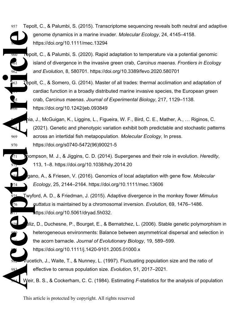
This article is protected by copyright. All rights reserved
957 Tepolt, C., & Palumbi, S. (2015). Transcriptome sequencing reveals both neutral and adaptive
958 genome dynamics in a marine invader. Molecular Ecology, 24, 4145–4158.
959 https://doi.org/10.1111/mec.13294
960 Tepolt, C., & Palumbi, S. (2020). Rapid adaptation to temperature via a potential genomic
961 island of divergence in the invasive green crab, Carcinus maenas. Frontiers in Ecology
962 and Evolution, 8, 580701. https://doi.org/10.3389/fevo.2020.580701
963 Tepolt, C., & Somero, G. (2014). Master of all trades: thermal acclimation and adaptation of
964 cardiac function in a broadly distributed marine invasive species, the European green
965 crab, Carcinus maenas. Journal of Experimental Biology, 217, 1129–1138.
966 https://doi.org/10.1242/jeb.093849
967 Thia, J., McGuigan, K., Liggins, L., Figueira, W. F., Bird, C. E., Mather, A., … Riginos, C.
968 (2021). Genetic and phenotypic variation exhibit both predictable and stochastic patterns
969 across an intertidal fish metapopulation. Molecular Ecology, In press.
970 https://doi.org/s0740-5472(96)90021-5
971 Thompson, M. J., & Jiggins, C. D. (2014). Supergenes and their role in evolution. Heredity,
972 113, 1–8. https://doi.org/10.1038/hdy.2014.20
973 Tigano, A., & Friesen, V. (2016). Genomics of local adaptation with gene flow. Molecular
974 Ecology, 25, 2144–2164. https://doi.org/10.1111/mec.13606
975 Twyford, A. D., & Friedman, J. (2015). Adaptive divergence in the monkey flower Mimulus
976 guttatus is maintained by a chromosomal inversion. Evolution, 69, 1476–1486.
977 https://doi.org/10.5061/dryad.5h032.
978 Véliz, D., Duchesne, P., Bourget, E., & Bernatchez, L. (2006). Stable genetic polymorphism in
979 heterogeneous environments: Balance between asymmetrical dispersal and selection in
980 the acorn barnacle. Journal of Evolutionary Biology, 19, 589–599.
981 https://doi.org/10.1111/j.1420-9101.2005.01000.x
982 Vucetich, J., Waite, T., & Nunney, L. (1997). Fluctuating population size and the ratio of
983 effective to census population size. Evolution, 51, 2017–2021.
984 Weir, B. S., & Cockerham, C. C. (1984). Estimating F-statistics for the analysis of population Acc
epte
d A
rtic
le

This article is protected by copyright. All rights reserved
985 structure. Evolution, 38, 1358–1370.
986 Welch, W. (1968). Changes in abundance of the green crab, Carcinus maenas (L .), in
987 relation to recent temperature changes. Fishery Bulletin, 67, 337–345.
988 Westram, A., Rafajlović, M., Chaube, P., Faria, R., Larsson, T., Panova, M., … Butlin, R.
989 (2018). Clines on the seashore: the genomic architecture underlying rapid divergence in
990 the face of gene flow. Evolution Letters, 2-4, 297–309. https://doi.org/10.1002/evl3.74
991 White, C., Selkoe, K. A., Watson, J., Siegel, D. A., Zacherl, D. C., & Toonen, R. J. (2010).
992 Ocean currents help explain population genetic structure. Proceedings of the Royal
993 Society B, 277, 1685–1694. https://doi.org/10.1098/rspb.2009.2214
994 White, T., Perkins, S., Heckel, G., & Searle, J. (2013). Adaptive evolution during an ongoing
995 range expansion: the invasive bank vole (Myodes glareolus) in Ireland. Molecular
996 Ecology, 22, 2971–2985. https://doi.org/10.1111/mec.12343
997 Wickham, H. (2016). ggplot2: Elegant Graphics for Data Analysis. Retrieved from
998 http://ggplot2.org
999 Wilson, J., Dormontt, E., Prentis, P., Lowe, A., & Richardson, D. (2009). Something in the way
1000 you move: dispersal pathways affect invasion success. Trends in Ecology and Evolution,
1001 24, 136–144. https://doi.org/10.1016/j.tree.2008.10.007
1002 Xuereb, A., Benestan, L., Normandeau, É., Daigle, R. M., Curtis, J. M. R., Bernatchez, L., &
1003 Fortin, M. J. (2018). Asymmetric oceanographic processes mediate connectivity and
1004 population genetic structure, as revealed by RADseq, in a highly dispersive marine
1005 invertebrate (Parastichopus californicus). Molecular Ecology, 27, 2347–2364.
1006 https://doi.org/10.1111/mec.14589
1007
1008 Data Accessibility1009 Raw transcriptome reads from new sequencing for this project have been deposited in
1010 GenBank’s Sequence Read Archive (SRA) under BioProject ID PRJNA690934 and
1011 BioSample IDs SAMN17267686-SAMN17267781. The cleaned transcriptome, high-quality
1012 individual SNP genotypes, and custom scripts used in this bioinformatics pipeline from in this Acc
epte
d A
rtic
le

This article is protected by copyright. All rights reserved
1013 paper will be archived in Dryad upon acceptance. Raw sequence reads from 2011,
1014 reanalyzed in this project, are available in the SRA under BioProject ID PRJNA283611 and
1015 BioSample IDs SAMN03653390-SAMN03653413.
1016
1017 Author Contributions
1018 All authors designed the research. CT performed research, analyzed data, and wrote the
1019 paper. All authors edited multiple drafts.
Acc
epte
d A
rtic
le

Tables
Table 1: Sampling information and summary statistics for each site x year sample. Adult = 1+ year old animal; YOY = Young of
the Year or <1 year old animal. Npoly = number of polymorphic SNPs; Ar = allelic richness; pAr = private allelic richness; HO =
observed heterozygosity; HE = expected heterozygosity; FIS = Wright’s inbreeding coefficient. All samples showed a significant
heterozygote excess (p < 0.05).
Code Site Coordinates Year Age N Npoly Ar pAr HO HE FIS
ES_15* Elkhorn Slough, CA 36.820, -121.745 2015 Adult 12 5,546 1.708 0.00697 0.2612 0.2510 -0.0409
SF_15* San Francisco Bay, CA 37.997, -122.370 2015 Adult 12 5,549 1.702 0.00621 0.2510 0.2491 -0.0078
SF_16 San Francisco Bay, CA 37.997, -122.370 2016 YOY 12 5,560 1.705 0.00666 0.2593 0.2501 -0.0365
SL_11 Seadrift Lagoon, CA 37.907, -122.662 2011 Adult 12 5,233 1.669 0.00494 0.2461 0.2414 -0.0196
SL_15* Seadrift Lagoon, CA 37.907, -122.662 2015 YOY 12 5,234 1.675 0.00584 0.2609 0.2424 -0.0761
SL_16 Seadrift Lagoon, CA 37.907, -122.662 2016 YOY 12 5,264 1.677 0.00434 0.2498 0.2442 -0.0228
BB_15* Bodega Bay, CA 38.324, -123.054 2015 Adult 12 5,538 1.706 0.00645 0.2681 0.2511 -0.0674
OR_16* Tillamook Bay, OR 45.542, -123.904 2016 YOY 12 5,548 1.711 0.00762 0.2618 0.2539 -0.0311
BC_11 Barkley Sound, BC 49.026, -125.346 2011 Adult 12 5,562 1.711 0.00771 0.2600 0.2520 -0.0316
BC_16* Barkley Sound, BC 49.026, -125.346 2016 Adult 12 5,517 1.705 0.00676 0.2630 0.2512 -0.0471
* indicates samples used in tests of selection and relative migration.
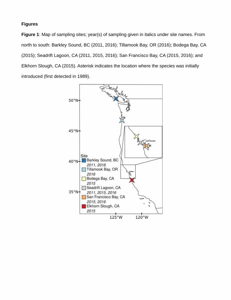
Figures
Figure 1: Map of sampling sites; year(s) of sampling given in italics under site names. From
north to south: Barkley Sound, BC (2011, 2016); Tillamook Bay, OR (2016); Bodega Bay, CA
(2015); Seadrift Lagoon, CA (2011, 2015, 2016); San Francisco Bay, CA (2015, 2016); and
Elkhorn Slough, CA (2015). Asterisk indicates the location where the species was initially
introduced (first detected in 1989).
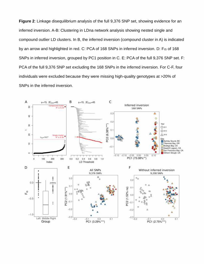
Figure 2: Linkage disequilibrium analysis of the full 9,376 SNP set, showing evidence for an
inferred inversion. A-B: Clustering in LDna network analysis showing nested single and
compound outlier LD clusters. In B, the inferred inversion (compound cluster in A) is indicated
by an arrow and highlighted in red. C: PCA of 168 SNPs in inferred inversion. D: FIS of 168
SNPs in inferred inversion, grouped by PC1 position in C. E: PCA of the full 9,376 SNP set. F:
PCA of the full 9,376 SNP set excluding the 168 SNPs in the inferred inversion. For C-F, four
individuals were excluded because they were missing high-quality genotypes at >20% of
SNPs in the inferred inversion.

44
Figure 3: Genetic structure, diversity, and migration across all sites, showing high gene flow
among all sites except Seadrift Lagoon. A: PCA of the independent 6,848 SNPs. B: PCA of
the putatively neutral 6,311 SNPs. C: Allelic richness by population and collection year across
the 6,848 independent SNPs, plotted against distance from the initial point of introduction in
San Francisco Bay, CA. Points from the same site have been jittered horizontally for clarity.
Vertical bars indicate standard error. Starred samples have significantly lower allelic richness
than non-starred samples. D: Relative migration between sites, calculated with the Nm
method, across the 6,662 independent SNPs in the five “open” sites. The highest observed
rate is set to 1, and all other rates are scaled to that maximum; estimated migration both into
and out of Seadrift was lower than migration between all other sites.

Figure 4: Comparison of isolation-by-distance (IBD) patterns across all open populations (excluding Seadrift Lagoon), showing
IBD driven by SNPs in the inferred inversion. A: For all 6,848 independent SNPs (red); 6,794 independent SNPs excluding the
large outlier LD cluster (gray); and 6,311 putatively neutral independent SNPs (black). B: For all 144 frequency outlier SNPs
across the open populations (aqua); and all 54 SNPs from the inferred inversion in the independent SNP set (blue). The
relationships in A are shown in B with smaller points; note the difference in Y-axis magnitude between the two panels.
Figure 5: Correlation between Minor Allele Frequency (MAF) and latitude or July SST at candidate genomic regions, showing
putative selection to temperature or latitude across the five “open” sites at environmental outlier SNPs. Asterisks indicate the
location where the species was initially introduced (first detected in 1989). In both cases, Seadrift Lagoon (gray point) is shown
for comparison but was not used in the regression lines or equations. A) The inferred inversion; samples were classed into
overall “inversion genotypes” based on their group membership in Figure 2C. B) Outlier SNP in the protein SGT homolog
transcript.