Banco Central de Chile Documentos de Trabajo

Central Bank of Chile Working Papers

N° 635

Julio 2011

TIME – CONSISTENT BAILOUT PLANS

Ernesto Pastén

La serie de Documentos de Trabajo en versión PDF puede obtenerse gratis en la dirección electrónica: http://www.bcentral.cl/esp/estpub/estudios/dtbc. Existe la posibilidad de solicitar una copia impresa con un costo de $500 si es dentro de Chile y US$12 si es para fuera de Chile. Las solicitudes se pueden hacer por fax: (56-2) 6702231 o a través de correo electrónico: bcch@bcentral.cl. Working Papers in PDF format can be downloaded free of charge from: http://www.bcentral.cl/eng/stdpub/studies/workingpaper. Printed versions can be ordered individually for US$12 per copy (for orders inside Chile the charge is Ch$500.) Orders can be placed by fax: (56-2) 6702231 or e-mail: bcch@bcentral.cl.

BANCO CENTRAL DE CHILE

CENTRAL BANK OF CHILE

La serie Documentos de Trabajo es una publicación del Banco Central de Chile que divulga los trabajos de investigación económica realizados por profesionales de esta institución o encargados por ella a terceros. El objetivo de la serie es aportar al debate temas relevantes y presentar nuevos enfoques en el análisis de los mismos. La difusión de los Documentos de Trabajo sólo intenta facilitar el intercambio de ideas y dar a conocer investigaciones, con carácter preliminar, para su discusión y comentarios. La publicación de los Documentos de Trabajo no está sujeta a la aprobación previa de los miembros del Consejo del Banco Central de Chile. Tanto el contenido de los Documentos de Trabajo como también los análisis y conclusiones que de ellos se deriven, son de exclusiva responsabilidad de su o sus autores y no reflejan necesariamente la opinión del Banco Central de Chile o de sus Consejeros. The Working Papers series of the Central Bank of Chile disseminates economic research conducted by Central Bank staff or third parties under the sponsorship of the Bank. The purpose of the series is to contribute to the discussion of relevant issues and develop new analytical or empirical approaches in their analyses. The only aim of the Working Papers is to disseminate preliminary research for its discussion and comments. Publication of Working Papers is not subject to previous approval by the members of the Board of the Central Bank. The views and conclusions presented in the papers are exclusively those of the author(s) and do not necessarily reflect the position of the Central Bank of Chile or of the Board members.

Documentos de Trabajo del Banco Central de Chile Working Papers of the Central Bank of Chile

Agustinas 1180, Santiago, Chile Teléfono: (56-2) 3882475; Fax: (56-2) 3882231

Documento de Trabajo Working Paper N° 635 N° 635

TIME – CONSISTENT BAILOUT PLANS‡

. Ernesto Pastén Banco Central de Chile

Visiting Fellow Toulouse School of Economics

Abstract Bailout policy is time-inconsistent, which results in multiple equilibria characterized by too much leverage, high risk correlation and little liquidity holding. I show that a long-run horizon allows the policy-maker to define bailout plans that rule out the worse equilibria. This result contrasts with the standard finding in environments with a unique equilibrium, as in most applications, in which a long-run horizon allows the policy-maker to support superior outcomes in equilibrium. I use this framework to discuss the effectiveness of three prudential policy proposals: too-big-to-fail size caps, taxes on borrowing and liquidity requirements. I also argue that policies alleviating the time-inconsistency of bailouts may generate large welfare gains. In this regard, I discuss three alternatives: policies against the scarcity of liquidity during crises, bailout design, and public debt. Resumen La inconsistencia temporal de la política de salvatajes financieros genera multiplicidad de equilibrios en los que los bancos tienen alto apalancamiento, alta correlación de riesgo entre ellos, y bajas provisiones de liquidez. En este artículo muestro que un horizonte de política de largo plazo permite a la autoridad financiera evitar la realización de los peores equilibrios. Esto contrasta con el resultado estándar en ambientes con un equilibrio único, como en la mayoría de las aplicaciones, en los que un horizonte de largo plazo permite a la autoridad generar equilibrios socialmente superiores. Complementariamente, utilizo mi marco teórico para analizar la efectividad de tres propuestas de política macro-prudenciales: restricciones al tamaño de los bancos, impuestos al endeudamiento, y requisitos mínimos de liquidez. También argumento que la reducción de la inconsistencia intertemporal de la política de salvatajes financieros genera grandes beneficios sociales, y propongo tres formas de lograrlo: políticas contra la escasez de liquidez durante las crisis, el diseño mismo de los salvatajes, y el rol de la deuda pública.

Email: epasten@cict.fr . Central Bank of Chile and Toulouse School of Economics. An earlier version of this paper has previously circulated under the title "Collective Moral Hazard, Liquidity Evaporation and Time-Consistent Bailouts". I thank insightful comments by Bruno Biais, Pablo D'Erasmo, Simon Gilchrist, Francisco Gonzalez, Pierre-Olivier Gourinchas, Chris Hellwig, Anton Korinek, Per Krusell, Enrique Mendoza, Giuseppe Moscarini, Guillermo Ordonez, Guillaume Plantin, Ricardo Reis, Randy Wright and seminar participants at the Central Bank of Chile, IIES, LUISS, Maryland, Toulouse and Yale. I specially thank Jean Tirole and Bob King. I also gratefully acknowledge editorial suggestions by Andrew Davis and Dan Schulte. The views expressed herein are those of the author and do not necessarily reflect the position of the Central Bank of Chile. Errors and omissions are my own.

1 Introduction

Kydland and Prescott (1977) uncovered a time-inconsistency problem of policy arising when

outcomes depend on expected policy: Even a benevolent authority breaks ex-post its promises

of "tough" policies, which in turn induces agents to take ex-ante actions that decrease social

welfare. Bailout policy also suffers from time inconsistency which induces banks’ moral haz-

ard in the form of high leverage, high risk correlation and little liquidity holding (Acharya

and Yorulmazer, 2007; Diamond and Rajan, 2009; Farhi and Tirole, 2009, 2010a). This

misbehavior has been pointed out at the core of the recent financial crisis.1 As a response, a

wide variety of prudential policies have been proposed to correct it–not to tackle its source.2

I study the time-inconsistency problem of bailouts when the authority takes into account

the future effect of its policy actions in a financial economy. Most of the related literature

focuses on static environments. Only Chari and Kehoe (2009) has the same focus, but my

financial environment–in which leverage, liquidity and risk correlation arise endogenously–

delivers sharply distinct results. Specifically, I apply sustainable plans (Chari and Kehoe,

1990) to bailout policy in an infinitely repetead version of Farhi and Tirole (2009, 2010a)–

who use the liquidity model of Holmstrom and Tirole (1998) to study the misbehavior of

banks when bailout policy lacks commitment. I use this framework to study three issues.

First, the ways in which a long-run policy horizon alleviates the time-inconsistency problem.

Second, to critically discuss three popular prudential policy proposals: too-big-to-fail size

caps (Chari and Kehoe, 2009), taxes on borrowing (Bianchi and Mendoza, 2010; Jeanne and

Korinek, 2011) and liquidity requirements (Farhi and Tirole, 2009, 2010a). Finally, to show

that policies tackling the time-inconsistency of bailouts have the potential to create large

welfare gains. In this regard, I discuss other three types of policy: the mitigation of the

scarcity of liquidity during crises, the design of bailouts, and public debt.

The baseline economy has entrepreneurs and households living three periods. Entrepre-

neurs can invest in risky and riskless assets while households can only invest in riskless assets.

Households thus lend to entrepreneurs to invest in risky assets, which have a higher return.

However, there is credit rationing since only a portion of future income is pledgeable. If a

"distress" state is realized in period two, risky assets need reinvestment; otherwise the assets

are lost. The more riskless assets entrepreneurs hold (liquidity), the more new loans they

get for reinvestment. Critically, an authority may "bailout" entrepreneurs by decreasing the

interest rate of loans at the cost of distorting households’ savings decisions.

1For instance, Diamond and Rajan (2008) and Brunnermeier (2009).2There is more than one source for this misbehavior; I focus on the time-inconsistency of bailouts.

1

Farhi and Tirole (2009, 2010a) show that there are no bailouts under commitment in this

economy. Entrepreneurs will hoard enough liquidity to ensure full reinvestment, which is the

constrained efficient outcome. Under discretion, many bailout policies are time-consistent,

including no bailouts. If a no-bailouts policy is defined ex-ante and agents believe it, then

no bailout is implemented ex-post. More broadly, any bailout policy is implemented ex-post

if agents ex-ante expect such a policy as long as the implied distortions on households are

not too large. The concavity of households’ utility creates an upper bound for the size of a

time-consistent bailout. Hence, inferior equilibria exist in which entrepreneurs leverage too

much, hoard too little liquidity and correlate their risk exposure such that they all need a

bailout at the same time, leading to the implementation of large distortionary bailouts.

I interpret this result as a time-inconsistency problem similar to the dams example in

Kydland and Prescott (1977): If agents expect no dams (bailouts) to be built (implemented)

on a flood plain (distressed economy), no houses are constructed there (enough liquidity is

hoarded), so dams (bailouts) are not necessary. But if houses are built in the flood plain (not

enough liquidity is hoarded), the authority will be forced to build the dams (to bail out).3

The problem then is not that the authority breaks its promises ex-post if agents believe them

ex-ante, as in most applications, but that promises are broken when larger-than-promised

bailouts are expected.4 Only the largest time-consistent bailout is "resistant" in the sense

that it is the only promise that is not broken to match expectations of even larger bailouts.

A natural question is whether reputation may substitute for commitment in this context.

I produce a non-overlapping generations economy such that each generation is a repetition

of the baseline model. This is the simplest way to introduce a long-run policy horizon, in

particular, I study sustainable plans (Chari and Kehoe, 1990). A bailout policy is sustainable

if the authority does not deviate from it when agents follow a trigger strategy: They believe

the plan if the authority has not previously deviated from its plans; otherwise they expect

the largest bailout under discretion. In other words, the authority suffers a fixed cost after

a deviation, which is interpreted as a reputation loss. I find that all time-consistent policies

in the baseline economy are sustainable. However, I also find that not only the largest

time-consistent bailout is "resistant". Hence, despite the fact that reputation does not help

to support better time-consistent policies, it does alleviates the time-inconsistency problem

since allows the authority to define plans that rule out the worse equilibria. Smaller time-

consistent bailout plans are "resistant" as the authority becomes more patient.

3Ennis and Keister (2009) show that a similar result holds for freezing deposits policy after a bank runin the Diamond and Dibvig (1983) banking economy.

4Promises are also broken when smaller-than-promised bailouts are expected, but this situation deliverssuperior equilibria.

2

Unfortunately, increasing the patience of an authority is a difficult task in practice. Hence

I focus on the case when the authority is not patient enough to make a no-bailout policy

resistant. This analysis delivers two main results. First, even a small reduction in resistant

bailout plans may create large welfare gains. This is because the concavity of households’

utility implies that the social cost of a bailout in each generation is convex in the size of

bailouts, and smaller bailouts increase current and future generations’ welfare. The second

result is that an exogenous reduction in the smallest resistant bailout plan is amplified by

a dynamic spillover. Given a plan, the fixed cost of a policy deviation is the difference in

future welfare when agents believe the plan and when they expect the largest bailout under

discretion. If a smaller bailout plan becomes resistant, the fixed cost of a policy deviation

increases, which implies that an even smaller bailout plan becomes resistant.

I then use this framework to study three popular prudential policy proposals. I show that

too-big-to-fail size caps (Chari and Kehoe, 2009) do not change the authority’s incentives

per se, so risk correlation implies that such a policy becomes ineffective if banks can cre-

ate new banks or increase the size of smaller banks. I also show that taxes on borrowing

(Bianchi and Mendoza, 2010; Jeanne and Korinek, 2011) may induce more borrowing if the

tax finances bailouts or its rebate is pledgeable. This is because the authority’s incentives

remain unaffected but entrepreneurs’ credit constraint is relaxed. Similarly, if the tax re-

duces households’ tax burden, the distortionary cost of bailouts decreases, worsening the

time-inconsistency problem and inducing more borrowing. In contrast, I show that liquidity

requirements still help even if circumvented by using toxic assets (Farhi and Tirole, 2009,

2010a) because such a policy helps to support smaller resistant bailout plans.

Finally, I also show that policy mitigating liquidity evaporation during crises–a sudden

scarcity of liquidity, such as the episode triggered after Lehman’s failure–alleviates time-

inconsistency. The design of bailouts, such as supporting the buyer banks but not the

failing banks (Acharya and Yorulmazer, 2007), reduces incentives to correlate risk and thus

alleviates the time-inconsistency. Public debt, a commonly suggested commitment device in

monetary policy (Persson, Persson and Svensson, 2006) and capital taxation (Dominguez,

2007), is also effective. However, these policies may not fully exploit the dynamic spillover

if they similarly affect the incentives of impatient and patient authorities.

Literature review. Most work uses static models to study banks’ misbehavior when pol-icy lacks commitment (Acharya and Yorulmazer, 2007; Farhi and Tirole 2009, 2010a) and

optimal bailout policy (Diamond and Rajan, 2009). I study time-consistent bailout policy

for a patient authority and its interaction with other policies. Despite I use Farhi and Ti-

role (2009, 2010a) as starting point, our goals are different. Only Chari and Kehoe (2009)

3

is similar in spirit to this paper, but not in the details. They apply sustainable plans to

bailout policy in a repeated economy where inefficient bankruptcies serve to discipline man-

agers. The authority bails out firms to avoids bankruptcies, which induces managers to

shirk. Their economy has a unique equilibrium policy under discretion; mine has multiple.

Hence they find the standard result that a long-run horizon allows the authority to sustain

better policies as equilibrium; I find that the authority can set plans that rule out the worse

equilibria. In addition, they conclude that a size cap solves the time-inconsistency problem;

I conclude that risk correlation–which is missing in their analysis–reverts this result. Their

paper also calls for ex-ante regulation to solve the time-inconsistency; I argue that policies

before, during or after crises help as long as they contribute to supporting smaller "resistant"

bailout plans. Finally, I study a richer variety of policies and point out that, if solving the

time-inconsistency is too ambitious, even a small alleviation may create large welfare gains.

Layout. Section 2 displays basic results in a one-generation model. Section 3 introducesinfinite generations and studies time-consistent bailout plans. Section 4 focuses on the three

prudential policies studied in this paper. Section 5 discusses how to alleviate the time-

inconsistency and Section 6 concludes. A notation table is added as an appendix.

2 Baseline model

This section follows Farhi and Tirole (2009, 2010a) to produce a one-generation model.

2.1 Setup

Consider a static economy with three stages, s = 0, 1, 2.5 There are two types of agents in

this economy, each with total mass one: households and entrepreneurs.

Households have exogenous endowments e0 and e1 in stages s = 0, 1 and utility

V = ch0 + u(ch1) + c

h2 ,

where ch0 , ch1 , c

h2 denotes consumption in stages s = 0, 1, 2 and u (·) satisfies u′ > 0, u′′ < 0.

Entrepreneurs have an exogenous endowment A only in stage s = 0 and utility

U = cent0 + cent1 + cent2 .

5Notation t is reserved for generations when this economy is infinitely repeated in Section 3.

4

There are two types of assets: riskless assets and risky assets. Riskless assets are available

for both households and entrepreneurs and simply transfer one unit of consumption across

stages. In contrast, only entrepreneurs can invest in risky assets. These assets provide a

gross return ρ1 > 1 in stage s = 2 if there is "no distress" in stage s = 1 (with probability

α). If there is "distress" in s = 1 (with probability 1− α), investment in risky assets is lostunless there is reinvestment in s = 1.6 Risky assets then provide ρ1 of gross return of the

reinvestment scale in s = 2. For either "no distress" or "distress" only a portion ρ0 < 1 of

the total expected returns is pledgeable.7

There is also an authority (for instance, a central bank), which can tax riskless investment

in s = 1, so its effective return is R ≤ 1. This tax is interpreted as a "bailout",8 which is

rebated via lump-sum transfers in s = 2. The authority’s objective is

V + βU

where β represents the relative weight of entrepreneurs’ welfare.

Timing. The timing of actions is as follows:

Stage s = 0: Households receive e0 and decide ch0 , how much to invest in the riskless asset

and to lend to entrepreneurs. Entrepreneurs receive A and decide cent0 , how much to invest

in risky assets i and in riskless assets xi.

Stage s = 1: Households receive e1 and the aggregate state of nature is revealed: "no

distress" (with probability α) and "distress" (with probability 1− α). In the distress state,households decide how much to invest in riskless assets and to lend to entrepreneurs for

reinvestment; entrepreneurs receive no endowment and decide their reinvestment scale j in

risky assets. In the no distress state, risky assets do not need reinvestment, so households

only invest in riskless assets. In either state, taxes on riskless assets are collected, and agents

choose ch1 and cent1 .

Stage s = 2: No one receives an endowment. Risky and riskless assets pay back, taxes are

rebated, and agents choose ch2 and cent2 .

Two cases will be studied: One in which the authority chooses R at s = 0, and another

in which R is chosen after the state is drawn at the beginning of s = 1.

6The distress state represents a scenario in which an aggregate liquidity shock hits the economy.7Limited pledgeability is assumed exogenous, but it may be justified by an optimal contract between

households and entrepreneurs that induce the latter to exert high effort (Holmstrom and Tirole, 1998).8Abusing a bit of notation, any policy R ≤ 1 is also called a bailout (of size 1−R).

5

2.2 Competitive equilibrium given policy

I solve for the equilibrium interaction between households and entrepreneurs treating policy

R and expected policy Re as exogenous variables. Later I use the results obtained here to

compute a reduced form of the authority’s objective to be used in the policy analysis.

Definition 1 Let R be the effective bailout policy implemented at stage s = 1 and Re be theexpected bailout policy at s = 0. A competitive equilibrium given {R,Re} is defined as thetriple {i (R,Re) , j (R,Re) , x (R,Re)} such that(i) Households maximize their utility V subject to their budget constraint.

(ii) Entrepreneurs maximize their utility U subject to their budget constraint.

(iii) The financial market clears.

In equilibrium Re = R. However, the equilibrium set is different depending on in which

stage the authority chooses R, either s = 0 or 1–to be studied respectively in Sections 2.3

and 2.4. The representation of the competitive equilibrium given policy R and expected

policy Re is an artifact that helps to simplify the subsequent analysis.

Given investment scale i and liquidity hoarding xi, entrepreneurs borrow from households

i+ xi− A,

the difference between their total investment in s = 0 and their endowment. Households’

endowment e0 is assumed large enough such that it is not binding. I also assume that

entrepreneurs invest all their endowment A in the risky asset (cent0 = 0), which is ensured by

1 + (1− α) < ρ1.

The break-even condition for households in s = 0 is

i+ xi− A = α (ρ0 + x) i. (1)

In words, households lend to entrepreneurs an amount equal to their total expected return.

Riskless investment has zero net return, so households ask for zero net return on loans.

Entrepreneurs repay to households only if there is no distress (because of limited liability),

in which case they pay their whole pledgeable income, (ρ0 + x) i.

6

The break-even condition implies that

i (x) =A

1 + (1− α) x− αρ0.

If the distress state is realized in s = 1, the reinvestment scale is

j (x,R, i) = min

{ρ0j + xi

R, i

}because (ρ0j + xi) is the maximum amount pledgeable by entrepreneurs in s = 1 and R is

the riskless after-tax return. Entrepreneurs have no incentive to increase scale above i, which

justifies the upper bound. Reinvestment may be further simplified to

j (x,R, i) = min

{x

R− ρ0, 1

}i

which depends on liquidity hoarding x as a proportion of the initial investment scale i, policy

R, and the portion ρ0 of future returns that is pledgeable.

Proposition 1 For α < 1, the competitive equilibrium given {R,Re} is characterized by

x (Re) = Re − ρ0.

i (Re) =A

1 + (1− α)Re − ρ0

j (R,Re) = min

{Re − ρ0R− ρ0

, 1

}i (Re)

Proof. Since payoffs are linear in the investment scale, the equation for x (Re) is obtainedby comparing the entrepreneurs’ expected payoff of holding no liquidity, x = 0, or holding

liquidity to ensure continuation at full scale for Re = R = 1. Equations for i (Re) and

j (R,Re) are obtained by substituting x (Re) into i (x) and j (x,R, i).

Note the different channels through which R and Re affect the equilibrium: R enters

directly only in reinvestment j; Re affects liquidity hoarding x and indirectly i and j.

2.3 Bailouts under commitment

I now turn to find the equilibrium bailout policy when the authority chooses R in s = 0, so

Re = R is internalized by the authority. The unique equilibrium has a no-bailouts policy.

7

Households’ welfare from stage s = 0 on is

V ex−ante (R,Re) = [e0 − i (Re)− x (Re) i (Re) + A]+α

[u(e1 − Snd

)+ Snd + (ρ0 + x (R

e)) i (Re)]

+(1− α) [u (e1 − Sd)+RSd + (1−R) [Sd − j (R,Re)]]The first term in brackets is households’ consumption at s = 0, which is the endowment

e0 minus the total lending to entrepreneurs. The second line is households’ consumption at

s = 1, 2 if there is no distress at s = 1. Investors utility at s = 1 is u(e1 − Snd

)and at s = 2

is the proceedings of their savings Snd (with zero net return) and of their s = 0 loans to

entrepreneurs, which yield ρ0+x (Re). The third line is households’ consumption at s = 1, 2

if there is distress at s = 1. Investors have utility u(e1 − Sd

)in s = 1, while at s = 2 the

proceedings of their savings RSd (including their investment in riskless assets and their new

loans to entrepreneurs, which both yield R ≤ 1), plus the rebate for the taxation on risklessinvestment, (1−R) [S − j (R,Re)].V ex−ante (·) may be further simplified by using the households’ break-even condition in

(1) and defining

V (R) = u (e1 − S) + S where u′ (·) = R. (2)

such that V (1) − V (R) is households’ welfare cost of a bailout R < 1, where V (R) is

increasing in R with V ′ (1) = 0 and V ′′ < 0. Thus,

V ex−ante (R,Re) = e0 + αV (1) + (1− α)[V (R)− (1−R) j (R,Re)

].

Ex-ante welfare for entrepreneurs may be represented by

U ex−ante (R,Re) = (ρ1 − ρ0) [αi (Re) + (1− α) j (R,Re)] .

Entrepreneurs consume at s = 2 all their non-pledgeable income. Their investment in

risky assets at s = 2 is i (Re) if there is no distress at s = 1 and j (R,Re) if there is distress.

Total ex-ante welfare is

W ex−ante (R,Re) = e0 + αV (1) + (1− α)[V (R)− (1−R) j (R,Re)

](3)

+β (ρ1 − ρ0) [αi (Re) + (1− α) j (R,Re)] .

where β is the weight of entrepreneurs in the financial authority’s objective.

8

Further, under commitment Re = R, so risky investment will always continue at full scale:

W ex−ante (R,R) = e0 + αV (1) + (1− α)[V (R)− (1−R) i (R)

]+ β (ρ1 − ρ0) i (R) .

This expression captures the negative effect on households’ welfare and the positive effect

on entrepreneurs’ welfare of a larger bailout (lower R). For households, a lower R distorts

more their savings (V (R) is smaller) and increases transfers to entrepreneurs in the distress

state ((1−R) i (R) is larger). LargerR increases entrepreneurs’ risky investment (i′ (R) < 0),and thus increases their consumption ((ρ1 − ρ0) i (R) is larger).

Proposition 2 There are no bailouts in equilibrium under commitment, R∗c = 1, if

β (ρ1 − ρ0) ≤ (1− α) + (1− ρ0) . (4)

Proof. Under condition (4), the overall effect of decreasing R on ex-ante welfare is negative.Thus, ∂W ex−ante(R,R)

∂R> 0 for R ≤ 1. ∂W ex−ante(R,R)

∂R< 0 for R > 1 because increasing R

distorts households’ saving decisions and also decreases risky investment.

This proposition defines a benchmark for the subsequent analysis.

2.4 Bailouts under discretion

I solve for the equilibrium bailout policy when the authority chooses R in s = 1, so the

authority takes Re as given. There is now a continuum of equilibrium bailout policies,

including the no-bailouts policy.

Following computations in Section 2.3 and the equation for j (R,Re) in Proposition 1, the

overall social welfare for stages s = 1, 2 if the distress state is realized is

W ex−post (R,Re) = V (R) + [β (ρ1 − ρ0)− (1−R)]Re − ρ0R− ρ0

i (Re) .

Given expectations Re, the authority chooses R = Re if

W ex−post (R,Re = R) ≥ W ex−post(R, Re = R

)∀R ≥ R. (5)

Proposition 3 The set of equilibrium bailouts under discretion is �d = [R, 1] such that

R ∈ �d satisfies [V(R)− V (R)

]≤ w R−R

R− ρ0i (R) ∀R ≥ R. (6)

9

when w = β (ρ1 − ρ0)− (1− ρ0) > 0. In addition, R ≥ ρ0

Proof. Condition (6) is the closed form of (5). R = 1 is an equilibrium; if Re = 1, then anypolicy R > 1 delivers lower ex-post welfare than R = 1 and R < Re is never optimal because

j = i ∀R < Re. The same argument applies for R ∈ [R, 1] because V (·) is concave withV ′ (1) = 0 and the right hand side of (6) is increasing in R for any R > ρ0. For R

e < R, the

cost of setting R = Re in terms of households’ welfare is higher than the benefit of reducing

entrepreneurs’ losses, so a policy R < R cannot be an equilibrium. R ≥ ρ0 because a policyR ≤ ρ0 ensures j = i.Discussion on time-inconsistency. Proposition 3 implies that, by construction, any

policy R ∈ �d is time-consistent. A promise of any policy R ∈ [R, 1] defined at s = 0 is

implemented at s = 1 when agents believe it at s = 0, i.e., Re = R. However, if agents

expect Re �= R, with Re ∈ �d, the authority deviates from R to implement Re.

The model therefore implies that there exists a time-inconsistency problem since the

authority cannot ensure that it will not break ex-post its promises made ex-ante. This

version of time-inconsistency is similar to the dams example in Kydland and Prescott (1977)

which is different from most applications. For instance, in the monetary policy or taxation

literatures the authority responds to low expected inflation (or low expected taxes) with

a high inflation policy (or high taxes). In bailout policy, the authority matches agents’

expectations. Thus, the problem is not that the commitment policy is not possible, but

that inferior policies from an ex-ante perspective are also possible. This paper focuses on

monetary bailouts to keep Farhi and Tirole (2009, 2010a) as a clean starting point, but a

similar analysis applies for fiscal bailouts.9 In particular, in this environment an inferior

policy means that in equilibrium there is too little liquidity, too much borrowing, large

distortionary bailouts, and risk correlation among entrepreneurs, which is introduced next.

2.5 Endogenous correlation of risk

I now sketch the argument proposed by Acharya and Yorulmazer (2007), Farhi and Tirole

(2009, 2010a) and Diamond and Rajan (2009). Risk correlation motivates the abstraction of

idiosyncratic risk in the model and is used in Section 4 to evaluate a too-big-to-fail policy.

Assume that there are two states of distress at stage 1: distress1 and distress2 such that

α1 + α2 = α,

9Farhi and Tirole (2009) also show that monetary policy is important in the optimal design of bailouts.

10

the probability of the economy being in distress is 1 − α. Also assume that entrepreneurschoose their exposure–the probability they need refinancing in a given state.

Proposition 4 There is a perfect correlation of risk exposure in equilibrium.

Proof. Let λ be the portion of the total investment that needs refinancing in distress1. Apolicy R belongs to the equilibrium set under discretion in distress1, �d,1, if

[V(R)− V (R)

]≤ λw R−R

R− ρ0i (R) ∀R ≥ R.

The inf {�d,1} is decreasing in λ and �d,1 → {R∗c} as λ → 0. Entrepreneurs are exposed to

the distress state in which R is lower. Since all entrepreneurs are identical, two equilibria

exist: λ = 1, �d,1 = [R, 1] and �d,2 = R∗c , and λ = 0, �d,1 = {R∗c} and �d,2 = [R, 1].Risk correlation arises because bailouts are untargetted and, given a level of liquidity

hoarding, larger bailouts are implemented when more risky investment needs refinancing.

3 Infinite policy horizon

I now extend the model to non-overlapping generations that preserves its three-stages struc-

ture but allows the authority to internalize the future effects of its actions. History-dependent

strategies introduce a fixed cost of a deviation from predetermined bailout plans. I then study

the effects of this fixed cost on the time-inconsistency problem of bailouts.

3.1 Modification of the baseline model

Consider an economy populated by generations of households and entrepreneurs. Each

generation lives for only one period t = 0, 1, ...,∞. Endowments remain exogenous andthere are no intergenerational transfers or state variables, so there is no interaction among

generations. Each period is broken into three stages s = 0, 1, 2, such that inside one period

the setup is identical to the baseline model of Section 2. There is again only one distress

state which gets revealed in stage s = 1 every period.

The competitive equilibrium in each period remains identical to Section 2 except that all

relevant variables are now indexed by t:

i (Ret ) =A

1 + (1− α)Ret − ρ0, (7)

11

x (Ret ) = Ret − ρ0, (8)

j (Rt, Ret ) = min

{Ret − ρ0Rt − ρ0

, 1

}i (Ret ) . (9)

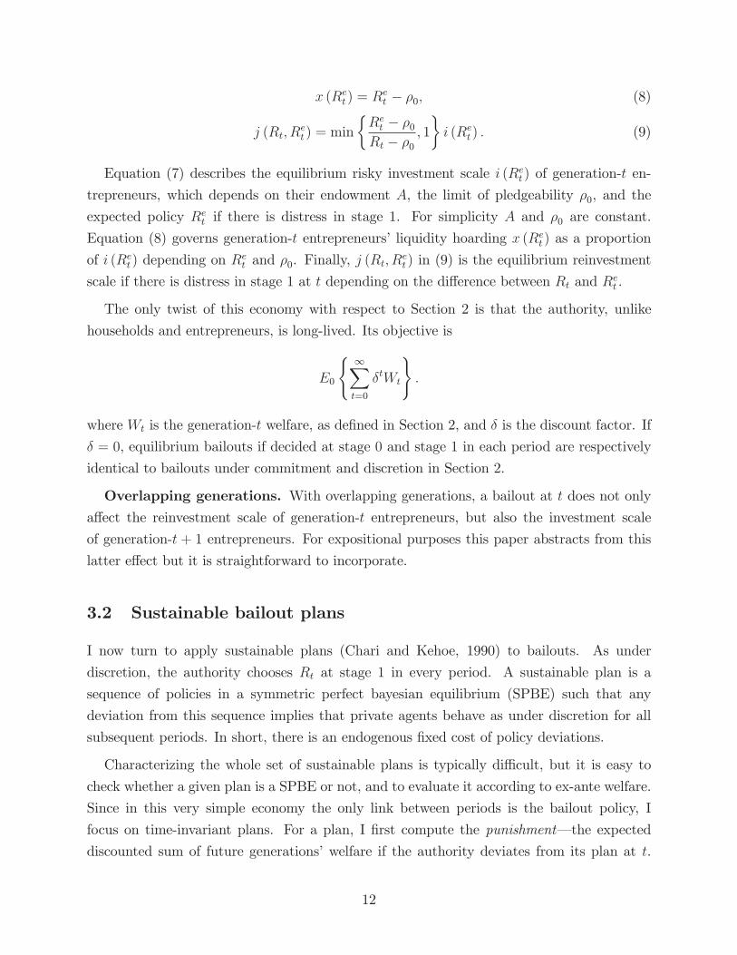
Equation (7) describes the equilibrium risky investment scale i (Ret ) of generation-t en-

trepreneurs, which depends on their endowment A, the limit of pledgeability ρ0, and the

expected policy Ret if there is distress in stage 1. For simplicity A and ρ0 are constant.

Equation (8) governs generation-t entrepreneurs’ liquidity hoarding x (Ret ) as a proportion

of i (Ret ) depending on Ret and ρ0. Finally, j (Rt, R

et ) in (9) is the equilibrium reinvestment

scale if there is distress in stage 1 at t depending on the difference between Rt and Ret .

The only twist of this economy with respect to Section 2 is that the authority, unlike

households and entrepreneurs, is long-lived. Its objective is

E0

{ ∞∑t=0

δtWt

}.

where Wt is the generation-t welfare, as defined in Section 2, and δ is the discount factor. If

δ = 0, equilibrium bailouts if decided at stage 0 and stage 1 in each period are respectively

identical to bailouts under commitment and discretion in Section 2.

Overlapping generations. With overlapping generations, a bailout at t does not onlyaffect the reinvestment scale of generation-t entrepreneurs, but also the investment scale

of generation-t + 1 entrepreneurs. For expositional purposes this paper abstracts from this

latter effect but it is straightforward to incorporate.

3.2 Sustainable bailout plans

I now turn to apply sustainable plans (Chari and Kehoe, 1990) to bailouts. As under

discretion, the authority chooses Rt at stage 1 in every period. A sustainable plan is a

sequence of policies in a symmetric perfect bayesian equilibrium (SPBE) such that any

deviation from this sequence implies that private agents behave as under discretion for all

subsequent periods. In short, there is an endogenous fixed cost of policy deviations.

Characterizing the whole set of sustainable plans is typically difficult, but it is easy to

check whether a given plan is a SPBE or not, and to evaluate it according to ex-ante welfare.

Since in this very simple economy the only link between periods is the bailout policy, I

focus on time-invariant plans. For a plan, I first compute the punishment–the expected

discounted sum of future generations’ welfare if the authority deviates from its plan at t.

12

Then I compute the reward–the expected discounted sum of future generations’ welfare

if the authority follows the plan at t and future generations expect the same policy. The

fixed cost of a deviation is the difference between the punishment and the reward, which is

compared to the current benefit of a deviation.

Punishment. I use the largest bailout under discretion to compute the punishment,

Rd = inf {�d}

where �d is defined in Proposition 3. This is a natural criterion given the nature of thetime-inconsistency problem at hand.

Since generations are identical, the punishment after a deviation at t is

punt (Rd) =W ex−antet (Rd, Rd)

1− δwhere ex-ante welfare is defined in (3). Note that risky investment continues at full scale.

Reward. Similarly, assuming that a given candidate plan R is an equilibrium, risky

investment continues at full scale, so the reward is

rewt (R) =W ex−antet (R,R)

1− δ .

Note that, in contrast to the punishment, the reward depends on the candidate plan R.

Definition 2 A sustainable equilibrium {it, xt, jt, Rt}∞t=0 is defined such that(i) {i (Ret ) , x (Ret ) , j (Rt, Ret )} form a competitive equilibrium given {Rt, Ret} according to

(7), (8) and (9).

(ii) A sustainable bailout plan R must satisfy, ∀R ≥ R and ∀t,

W ex−postt (R,Ret = R) + δrewt+1 (R) ≥ W ex−post

t

(R, Ret = R

)+ δpunt+1 (Rd) (10)

The left-hand side of (10) is social welfare from stage s = 1 at t if the plan R = Ret

is carried out at t. The right-hand side of (10) is social welfare from stage s = 1 at t if

the authority deviates at t to R when Ret = R. Intuitively, a bailout plan is sustainable if

the authority does not deviate from it when agents believe the plan and their behavior is

13

sequentially rational (ensured by condition (i)). Since a policy Rt < Ret distorts households’

consumption without increasing reinvestment scale, plans R < R are excluded from (10).

Proposition 5 A bailout plan R ∈ �s, the set of sustainable bailout plans, if[V(R)− V (R)

]− ω R−R

R− ρ0i (R) ≤ δ [rewt+1 (R)− punt+1(Rd)] ∀R ≥ R, ∀t (11)

where �d ⊆ �s.

Proof. (11) follows form (10). �d ⊆ �s since rewt+1 (R)− punt+1(Rd) ≥ 0 for R ∈ �d.Condition (11) may be compared to (6) under discretion. The left-hand side of (11)

represents the current benefit of a policy deviation to a smaller-than-planned bailout. The

right-hand side is the fixed cost of the deviation in terms of future generations’ welfare due

to the realization of an inferior equilibrium from an ex-ante perspective.

Discussion on time-inconsistency. The result that �d ⊆ �s is standard in the litera-ture of sustainable plans, but here it has important implications. As discussed in Section 2.4,

the time-inconsistency problem of bailout policy is different than in most applications: It is

not that a promise of a "tough" policy is ex-post broken when agents believe it ex-ante, but

that this promise is broken when agents do not believe it. In particular, inferior equilibrium

outcomes take place when agents expect larger-than-promised bailouts.

Since the optimal policy under commitment, no bailouts, is already time-consistent for an

impatient authority (Proposition 3), such a policy is also time-consistent when the authority

has a long-run policy horizon. Thus, reputation does not help to support time-consistent

bailout policies that are superior from an ex-ante perspective, as in most applications. How-

ever, I show in the following that reputation still alleviates the time-inconsistency problem.

3.3 "Resistant" time-consistent bailout plans

Assume that the authority announces a bailout plan at the beginning of stage 0 every period

but the bailout policy is still decided in stage 1. Entrepreneurs and households, in turn, play

the same trigger strategy as above: They trust the plan if the authority has not deviated

in previous generations, but expect the realization of the largest equilibrium bailout under

discretion if the authority has deviated. In this context, I define "resistant" time-consistent

bailout plans, identify the best policy in this set, and study its properties.

14

Definition 3 A sustainable bailout plan R is also "resistant" if, ∀Ret ∈ [Rd, R] and ∀t,

W ex−postt (R,Ret ) + δrewt+1 (R) ≥ W ex−post

t (Ret , Ret ) + δpunt+1 (Rd) . (12)

That is, a resistant plan satisfies two conditions. It is sustainable, so it is time-consistent.

In addition, the plan is not abandoned if agents expect a larger-than-planned bailout, pro-

vided that the expected bailout is also sustainable. This latter requirement implies that if

the authority deviates from the plan, the authority matches expectations.

I now turn to study some basic properties of the best "resistant" time-consistent plan R∗s.

Proposition 6 The plan R∗s is such that

(i) R∗s is the highest bailout policy R that satisfies, ∀Ret ∈ [Rd, R] and ∀t,[V (R)− V (Ret )

]− ωR−R

et

R− ρ0i (Ret ) ≥ δ [punt+1(Rd)− rewt+1 (R)] (13)

(ii) R∗s is increasing in δ ≤ δ such that R∗s → Rd as δ → 0 and R∗s → R∗c as δ → δ.

(iii) While some plans R > 1 are resistant for δ > δ, they are ex-ante inferior than R∗c .

Proof. (i) Inequality (13) is the closed form of (12). R∗s is the highest policy R ≤ 1 that

satisfies this condition because the optimal ex-ante policy is R∗c = 1.

(ii) If δ = 0, (10) is identical to (5) and (12) collapses to

W ex−postt (R,Ret ) ≥ W ex−post

t (Ret , Ret ) ∀Ret ∈ [Rd, R] ,∀t

which is only consistent with (5) for R = Rd.

For δ > 0, the left and the right-hand sides of (13) become negative for any R > Rd. As

V ′ > 0 and V ′′ < 0, the right-hand side decreases more for some R > Rd. Hence (13) is

satisfied for some R > Rd. Since the optimal ex-ante policy is R∗c = 1, R∗s > Rd. Given

the definition of the reward and punishment, their difference for R > Rd goes to infinity as

δ → 1. In contrast, the left-hand side of (13) does not depend on δ. Thus, R∗s is increasing

in δ with R∗s = R∗c = 1 for some δ = δ.

(iii) δ > δ implies that some negative bailouts R > 1 are sustainable and satisfy (13).

However, such policies are ex-ante suboptimal with respect to R∗c by definition.

Proposition 6 obtains a closed form of the condition for a sustainable plan to be resistant

(Definition 3). This closed form is used extensively in the subsequent analysis. The best

15

resistant plan from an ex-ante perspective is the highest R since ex-ante welfare is increasing

in R = Re with a maximum at R = 1 (Proposition 2). Another important point is that the

only "resistant" plan for an impatient authority (δ = 0) is the lowest time-consistent policy

Rd. Such policy is the only one that is not abandoned to match larger-than-planned bailouts

since any policy R < Rd is not an equilibrium. However, as δ increases, higher policies R

become resistant. As δ increases, the fixed cost of a policy deviation increases, so higher R

are resistant to expectations of larger-than-planned bailouts. In addition, the best resistant

bailout plan is increasingly monotone in δ. The concavity of households’ utility implies that

cost in terms of households’ welfare of a deviation from the plan is smaller as the size of the

planned bailout is also smaller (higher R < 1). Since the fixed cost of a deviation goes to

infinity, a no-bailouts policy (R = 1) is a resistant plan for δ ≥ δ < 1.Because in practice it is difficult to increase the patience of the authority, I focus on the

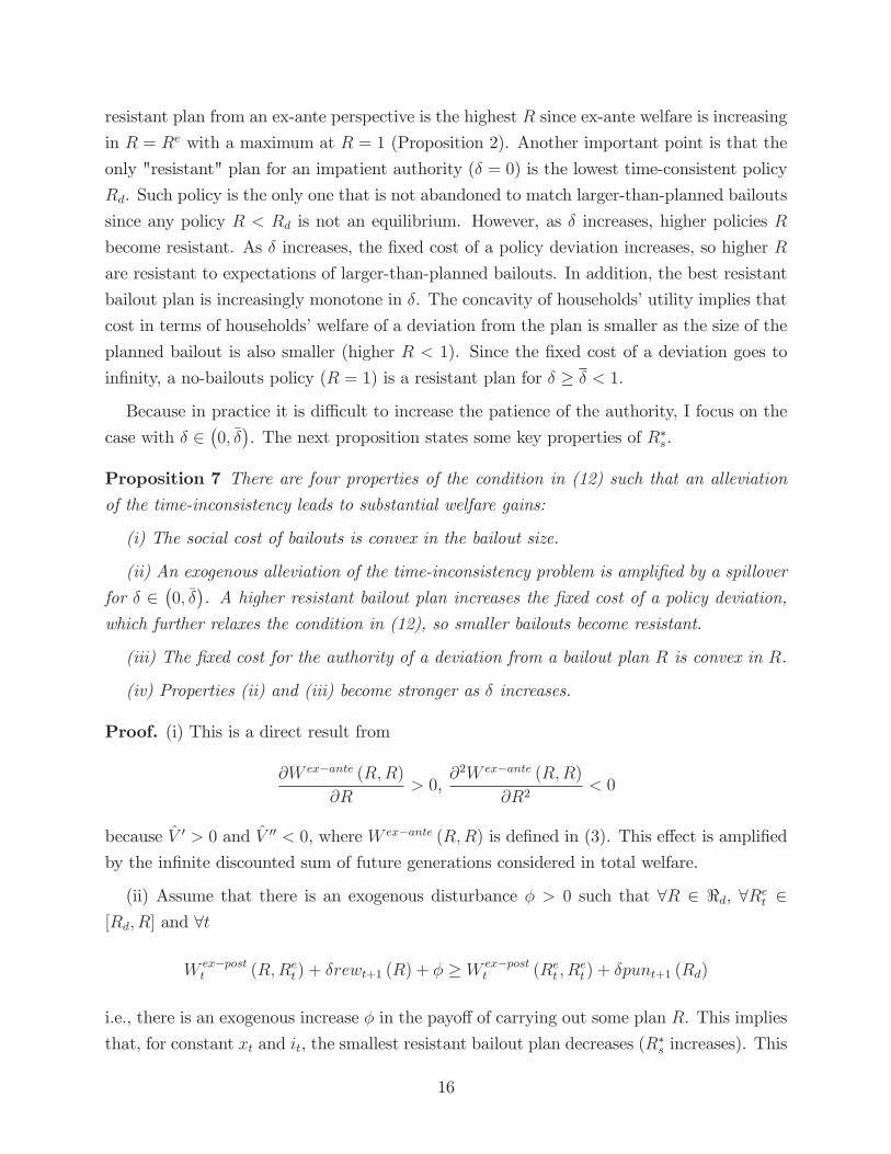
case with δ ∈ (0, δ). The next proposition states some key properties of R∗s.Proposition 7 There are four properties of the condition in (12) such that an alleviationof the time-inconsistency leads to substantial welfare gains:

(i) The social cost of bailouts is convex in the bailout size.

(ii) An exogenous alleviation of the time-inconsistency problem is amplified by a spillover

for δ ∈ (0, δ). A higher resistant bailout plan increases the fixed cost of a policy deviation,which further relaxes the condition in (12), so smaller bailouts become resistant.

(iii) The fixed cost for the authority of a deviation from a bailout plan R is convex in R.

(iv) Properties (ii) and (iii) become stronger as δ increases.

Proof. (i) This is a direct result from

∂W ex−ante (R,R)∂R

> 0,∂2W ex−ante (R,R)

∂R2< 0

because V ′ > 0 and V ′′ < 0, where W ex−ante (R,R) is defined in (3). This effect is amplified

by the infinite discounted sum of future generations considered in total welfare.

(ii) Assume that there is an exogenous disturbance φ > 0 such that ∀R ∈ �d, ∀Ret ∈[Rd, R] and ∀t

W ex−postt (R,Ret ) + δrewt+1 (R) + φ ≥ W ex−post

t (Ret , Ret ) + δpunt+1 (Rd)

i.e., there is an exogenous increase φ in the payoff of carrying out some plan R. This implies

that, for constant xt and it, the smallest resistant bailout plan decreases (R∗s increases). This

16

also implies that the reward term rew(R) increases, which decreases the right-hand side of

(13). This second-round effect further increases R∗s.

(iii) This is a direct result of (i) and the definition of the reward and punishment.

(iv) The right-hand side of (13) is convex in δ. Hence, the effect of φ on the right-hand

side of (13) is higher as δ increases. However, R∗c is also increasing in δ, which when combined

with the property (i) in this proposition may mitigate the overall effect.

Proposition 7 has important policy implications. When social discounting δ ∈ (0, δ), itimplies that the interaction between any change in financial regulation or policies and the

time-inconsistency problem of bailouts may be relevant in evaluating the overall effect of

these policy changes. Proposition 7 also stresses that some financial policies may be useful

in alleviating the time-inconsistrency problem of bailouts (discussed in Section 5). This is

because the size of bailouts is intrinsically linked to the incentives of entrepreneurs to hoard

liquidity, and thus to welfare. Property (i) in Proposition 7 states that smaller bailouts

produce large welfare gains. Property (ii) shows that smaller time-consistent bailouts imply

a higher cost of a current policy deviation, so even smaller bailouts may be supported.

Property (iii) states that the fixed cost of a deviation from the plan is convex in the difference

between the smallest resistant plan and the largest bailout under discretion. Property (iv)

shows that this fixed cost is also convex in δ.

Discussion on time-inconsistency. The results in this section imply that, if a time-consistent plan R > Rd is resistant, then defining ex-ante such a plan implies that all

equilibria in which the bailout is larger than planned are ruled out. This limits the extent

in which over-leverage, little liquidity hoarding and distortions in households’ decisions take

place in equilibrium. Note that resistant plans may still be abandoned when agents expect

smaller-than-planned bailouts, but ex-ante welfare is higher than what the plan delivers.

Hence, these deviations are not in the spirit of Kydland and Prescott (1977). Summing

up, reputation helps to alleviate the time-inconsistency problem of bailout policy, but the

mechanism is different than in most applications.

This section has another important result: Policies helping to support smaller resistant

bailouts plans may be amplified by an implicit dynamic spillover (property (ii) in Proposition

7). Most prudential policy proposals focus on correcting banks’ behavior. Instead, this result

suggest that prudential policy should focus on tackling the time-inconsistency of bailout

policy. In what follows, I first critically evaluate three popular prudential policy proposals

and later I elaborate on which types of policies can support smaller resistant bailouts plans.

17

4 A critical view to prudential policy

This section highlights the importance of evaluating financial policies taking into account

their interaction with the time-inconsistency problem of bailouts. Two commonly suggested

types of prudential policy–too-big-to-fail size caps and taxes on borrowing–may become

largely ineffective in this context. In contrast, some authors have shown concern that another

popular prudential policy, liquidity requerements, becomes ineffective if banks use toxic assets

to fool the regulator. I show that this policy still has an indirect positive effect by alleviating

the time-inconsistency problem of bailouts.

4.1 Too-Big-to-Fail size caps

Chari and Kehoe (2009) argue that limiting the size of banks reduces the incentives of the

authority to bailout, and thus alleviates its time-inconsistency problem. However, when

there is an endogenous correlation of risk among banks, I show that a size cap is ineffective

in equilibrium if there is a frictionless flow of capital among banks.

Let i∗ be a cap on risky investment scale, it (Ret = 1) ≥ i∗, with it (Ret ) defined as in (7).Let

A∗ (Ret , i∗) = [1 + (1− α)Ret − αρ0] i∗

be the level of "capital" according to (7) such that the desired investment scale i (Ret ) equals

the cap i∗. A∗ (Ret , i∗) is increasing in Ret because as R

et increases entrepreneurs hoard more

liquidity, so more capital is needed to attain scale i∗.

Given the size cap i∗, entrepreneurs’ idle capital is A − A∗ (Ret , i∗). If entrepreneurs areallowed to use this capital to open another, potentially smaller bank, the total amount of

risky investment in the economy is

i∗ + i (Ret , A− A∗ (Ret , i∗)) .

Assuming for simplicity that A ≤ 2A∗ (ρ0, i∗) and defining i

(Ret , A

)as the size of a firm

with capital A:

i(Re, A

)=

A

1 + (1− α)Re − ρ0.

By definition i (Ret , A∗ (Ret , i

∗)) = i∗, so total investment is

i (Ret , A)

18

which is independent of the cap i∗ and equals the total desired investment. Large and small

banks may have different investment strategies, but the they all have incentive to get exposed

to the same distress state. The total amount of resources under distress that need refinancing

is what matters for the time-consistency of bailouts. Hence, a too-big-to-fail policy fails at

alleviating the time-inconsistency. Of course, if there are frictions in the flow of capital

among banks, size caps will have an effect through reducing the size of risky investment by

a similar mechanism to that operating for liquidity requirements (Section 4.3).

4.2 Taxes on borrowing

This proposal has two motivations. One is the informal argument that banks should pay

ex-ante for the insurance they get ex-post in the form of bailouts. The other, formally

analyzed, proposes a Pigouvian correction of an externality that leads to overborrowing

(Bianchi and Mendoza, 2010; Jeanne and Korinek, 2011). This externality arises because

one borrower hitting their borrowing constraint tightens other borrowers’ constraints in

general equilibrium when credit rationing depends on the value of collateral. The model in

this paper is too simple to capture this externality, but it suffices to show that there is a

force inducing overborrowing in the interaction of taxes, the borrowing constraint, and the

time-inconsistency problem of bailouts.

This interaction may take two forms. For the first, consider a proportional tax on risky

investment τ to be collected at stage s = 0 in every period t. Assume that the tax collected

is rebated to entrepreneurs at stage s = 2. Households’ break-even condition is now

it + xtit + τ tit − A = α (ρ0 + xt + τ) it

because the total amount borrowed by entrepreneurs includes the tax amount τit and the tax

rebate is pledgeable income. Thus, households receive at stage s = 2 the rebate as payment

for their loans to entrepreneurs at s = 0 if there is no distress at s = 1 (with probability α).

Hence, risky investment scale is

it (xt, τ) =A

1 + (1− α) (xt + τ)− αρ0.

It initially appears that the tax decreases investment scale, but this effect vanishes in

equilibrium. Since the tax rebate is pledgeable, entrepreneurs can use it to get funding for

19

reinvestment if there is distress at s = 1. Thus, the reinvestment scale is

jt = min

{xt + τ

Rt − ρ0, 1

}it.

Focusing on the parameter subspace in which entrepreneurs choose liquidity hoarding to

ensure the continuation of their risky investment at full scale,

xt = Ret − ρ0 − τ .

The tax decreases entrepreneurs’ liquidity hoarding xt such that risky investment it re-

mains constant. Therefore, the equilibrium set of discretionary or sustainable monetary

bailouts remain identical. A tax on borrowing becomes ineffective because the authority’s

incentives to bailout remain unaffected, while entrepreneurs foresee that their credit con-

straint for reinvestment is relaxed. As a result, entrepreneurs cut their liquidity hoarding

(i.e, increase their borrowing) exactly in the amount raised by the tax.

Alternatively, assume that the tax is not rebated to entrepreneurs, so it is not pledgeable,

but transferred to households. The mechanism is now different but the result is similar.

Assume that households are also taxed to finance an exogenous and constant level of public

spending g. Since the only concave component in households’ utility is at stage s = 1, assume

that the tax ζ is also levied from the return on riskless investment. Households’ saving at

s = 1 is now determined by

u′ (e1 − St) = (1− ζ)Rt.

where ζ satisfies ζSt = g and Rt ≤ 1 is the bailout under distress at stage s = 1.If the amount levied from entrepreneurs τit is used to finance g, the tax on households

must satisfy ζSt = g − τit. Hence, ζ is decreasing in τ . The lower is ζ, the lower is also thecost of the bailout Rt ≤ 1 on distorting households’ consumption decisions. Therefore, a taxon entrepreneurs’ borrowing reinforces the time-inconsistency problem of bailouts if this tax

decreases households’ tax burden. Since this analysis is similar to the introduction of public

debt, the details are delayed to Section 5.3.

4.3 Liquidity requirements

I first sketch an argument on why this policy is considered ineffective. Consider a liquidity

requirement proportional to risky investment x ≥ 1 − ρ0 such that it is binding for anyRet ∈ [Rd, 1]. Assume that there is a cheaper form of liquidity called "toxic assets" with

20

price p < 1. Denote the investment of a entrepreneur at t in toxic assets as ytit. Toxic assets

pay 1 unit of the good in the no-distress state and pay 0 in the distress state (in contrast

to riskless assets, which pay 1 in either state). Critically, assume that the authority cannot

distinguish between both forms of liquidity, so

xt + yt ≥ x.

Given the policy x, entrepreneurs’ optimal choice is

xt = Ret − ρ0,yt = x− xt.

Entrepreneurs hold riskless assets up to their desired level of liquidity and use toxic assets

to meet x. Therefore, the refinancing capacity of entrepreneurs in the state of distress is

identical to the case without the liquidity requirement. This is because the time-inconsistency

problem of bailouts provides incentives to entrepreneurs to hold too little liquidity. The

policy x works as a restriction; entrepreneurs try to circumvent it.

This result is due to in Farhi and Tirole (2009). However, a positive indirect effect absent

in their work is that x decreases risky investment scale. This allows the authority to support

smaller resistant time-consistent bailouts. To see this, generation-t households’ break even

condition is now

it + xtit + pytit − A = α (ρ0 + xt + yt) it,

which implies

it (xt, x) =A

1 + (1− α) xt − αρ0 + (p− α) (x− xt).

Hence it (xt, x) is weakly smaller than it (xt) in (7) if p > α. How much smaller depends

on how restrictive x is with respect to the desired level of liquidity hoarding xt.

Let it (Ret , x) be the investment scale given expected bailouts Ret and liquidity requirement

x. The condition in (13) for a time-consistent bailout to become resistant is[V (R)− V (Ret )

]− ωR−R

et

R− ρ0it (R

et , x) ≥ δ [punt+1(Rd, x)− rewt+1 (R, x)]

Since it (Ret , x) < it (Ret ) ∀Ret ∈ [ρ0, 1), x introduces an exogenous alleviation of this

condition. Proposition 7 applies and hence R∗s is increasing in x. The only caveat is that Rdis also increasing in x, which partially offsets the spillover shown in Proposition 7 because a

21

higher Rd reduces the fixed cost of a deviation from a bailout plan. However, bailouts under

discretion do not exhibit a spillover effect, hence R∗s is increasing more rapidly than Rd in x.

Discussion on time-inconsistency. The goal of these three policy proposals is to

correct banks’ (entrepreneurs’) misbehavior, but they fail to tackle its source in the time-

inconsistency problem of bailouts. A too-big-to-fail size cap fails because ignores endogenous

risk correlation.

The motivation for taxes on borrowing appears after an externality arising in general

equilibrium when there is credit rationing (Bianchi, 2011), which induces over-borrowing. I

show above two warnings regarding with policy. First, both papers studying the correction of

this externality via taxes, Bianchi and Mendoza (2010) and Jeanne and Korinek (2011), use

a reduce form for the functional form of credit rationing. I show that taxes (and specifically,

rebates) change the payoff profile of borrowers, and thus change the terms of loan contracts.

Hence, a tax on borrowing decreases the incentives to borrow, but the rebate relaxes the

credit constraint without changing the authority’s incentives to bailout. Not rebating the

tax revenue may also induce borrowing if such revenues decrease the distortionary costs of

bailouts. Once again, these results stress the importance of evaluating prudential policy

proposals taking into account their effects on the time-inconsistency problem of bailouts.

My results regarding liquidity requirements also highlight the interplay between financial

policies and the time-inconsistency problem of bailouts. In particular, some policies alleviate

the time inconsistency, and thus provide deep incentives to banks (entrepreneurs) to align

their behavior with the social interest. The next section elaborates on this point.

5 Exploiting resistant bailout plans

I now propose three policies that have the potential of making smaller time-consistent bailout

plans resistant. Hence the authority can avoid the realization of worse equilibria. Specifically,

I discuss the effect of liquidity evaporation, the design of bailouts, and the role of public debt.

5.1 Liquidity evaporation

Liquidity evaporation refers to any spillover mechanism during financial crises that leads

short-run securities markets to freeze, haircuts and collateral requirements dramatically in-

crease, etc.; in short, a sharp increase in the liquidity premium or a sudden scarcity of

liquidity. There are a number of potential mechanisms for these phenomena, each labelled

22

by a different name.10 To examine the implications of liquidity evaporation, instead of fo-

cusing on any specific mechanism, I simply assume that households ask for an exogenous

premium q > 1 over the riskless interest rate if entrepreneurs are forced to downsize the

scale of their risky investment. Alternative assumptions with similar results are an exoge-

nous decrease in pledgeability ρ0, a destruction of liquidity hoarding on xt, or a decrease in

the liquidation value of risky assets (after relaxing zero liquidation value).

Under this assumption, risky investment scale i (Ret ) and liquidity hoarding x (Ret ) remain

identical to equations (7) and (8). This is because downsizing is an off-equilibrium event.

The only difference is that reinvestment scale is now

j (Rt, Ret ; q) =

{i (Ret ) if Rt ≤ Ret ;

Ret−ρ0qRt−ρ0 i (R

et ) if Rt > Ret .

If the bailout is equal or larger than expected (Rt ≤ Ret ), risky investment continues at fullscale. However, if the bailout is smaller than expected (Rt > Ret ), entrepreneurs must pay a

premium q > 1 over the after-tax return of the riskless asset to borrow from households.

Thus, a time-consistent policy R must satisfy the following condition to become resistant,

∀Ret ∈ [Rd, R],

[V (R)− V (Ret )

]− ωqR−R

et

qR− ρ0i (Ret )− (q − 1)

Ret − ρ0qR− ρ0

Ri (Ret ) ≥ δ[punt+1 (Rd)

−rewt+1 (R)

](14)

The key distinction of (14) with respect to (13) is on the left hand side of the inequality.

Given policy R, liquidity evaporation affects welfare in two opposite ways. Entrepreneurs

must pay a premium q > 1 over the interest rate R to obtain liquidity, so they are forced

into larger downsizing. But larger downsizing implies larger rebates to households because

rebates are proportional to the tax revenue. Thus, given policy R, the larger is entrepreneurs’

downsizing, the more households invest in the riskless asset, so rebates are larger. The overall

effect on welfare is negative under the assumption in (4). However, another effect is that Rdalso increases when q is smaller, which decreases the resistance of bailouts plans.

Therefore, policies mitigating liquidity evaporation may have strong effects on the incen-

10These mechanisms are not fully independent of each other. Some examples are bank runs (Diamondand Dibvig, 1983), contagion (Allen and Gale, 2000), rollover risk (Acharya, Gale and Yorulmazer, 2010),panic (Dasgupta, 2004), liquidity black holes (Morris and Shin, 2004), predatory trading (Brunnermeierand Pedersen, 2005), liquidity spirals (Brunnermeier and Pedersen, 2009), Knightian uncertainty (Caballeroand Krishnamurthy, 2008; Caballero and Simsek, 2010), bubbly liquidity (Farhi and Tirole, 2010b), andself-fulfilling credit freezes (Bebchuk and Goldstein, 2011).

23

tives to hoard liquidity. However, to explore this possibility, it is first needed to identify

which of the mechanisms for liquidity evaporation in footnote 10 are most relevant empiri-

cally. For instance, Woodford (1990) pointed out that public debt may serve as a vehicle to

create liquidity in the economy. If such a policy is effective in reducing liquidity evaporation,

Proposition 7 implies that this policy will also produce large effects on reducing entrepre-

neurs’ incentives to overborrow by alleviating the time-inconsistency problem of bailouts.

5.2 The design of bailouts

A key assumption to obtain the perfect correlation of risk exposure in equilibrium is that

bailouts are untargetted policy–i.e., it does not discriminate among banks. However, the

exact design of a bailout plan may generate different incentives in different types of banks

that may break the correlation.

For instance, Acharya and Yorulmazer (2006) show that there is a trade-off in banks’

decision to correlate risk: The higher the correlation, the larger the bailout is in equilibrium–

as sketched in Section 2.5, but a bank that does not correlate its risk with other banks may

take advantage of the inefficient liquidation of assets under distress (after relaxing zero

liquidation value, as assumed throughout this paper.)

If this assumption is relaxed, a bailout design that facilitates the access to liquidity not of

the failing banks, but of the buyer banks decreases the benefit of risk correlation, which may

provide enough incentives for banks to uncorrelate their exposition. Acharya and Yorulmazer

(2006) show that this incentive is stronger for bigger banks. My results complement their

conclusion by pointing out that the design of bailouts may not only break the correlation of

risk exposure, but also reduce the incentives for overborrowing.

5.3 The role of public debt

Section 4.3 implicitly conveys the idea that raising households’ tax burden increases the dis-

tortionary cost of bailouts. Thus, higher distortionary taxes alleviate the time-inconsistency

problem. Public debt has the property that affects tax burden but it is predetermined with

respect to the bailouts implementation. Thus, public debt works as a state variable in the

authority’s time-inconsistency problem. Hence, taxation to repay public debt is unrelated

to the authority’s problem to set and implement bailout plans. The use of public debt as a

commitment device is not novel to this paper; it has been used in the contexts of monetary

and fiscal policy such as in Persson, Persson and Svensson (2006) and Dominguez (2007).

24

Similarly to Section 4.3, assume that a tax rate ζ on the return to riskless investment at

stage s = 1 in every period t is used to pay g, now interpreted as the service of public debt.

The tax rate is such that ζSt = g, where St is determined by u′ (e1 − St) = (1− ζ)R, withR = 1 in the no-distress state and R ≤ 1 in the distress state.Then, the time-consistency condition for a bailout plan R ∈ �s is, ∀Ret ∈ [Rd, R],[

V (R, ζ)− V (Ret , ζ)]− ωR−R

et

R− ρ0it (R

et ) ≥ δ [punt+1(Rd, ζ)− rewt+1 (R, ζ)] (15)

where

punt+1(Rd, ζ) =1

1− δ[e0 + αV (1, ζ) + (1− α)

[V (Rd, ζ)− (1−Rd) i (Rd)

]+ β (ρ1 − ρ0) i (Rd)

],

rewt+1(R, ζ) =1

1− δ[e0 + αV (1, ζ) + (1− α)

[V (R, ζ)− (1−R) i (R)

]+ β (ρ1 − ρ0) i (R)

],

V (R, ζ) = u (e1 − St) + St such that u′ (e1 − St) = (1− ζ)R.

The tax ζ is levied regardless of whether there is distress or not. Given the properties

of V (R) in (2), V (·) is concave and increasing in (1− ζ)R < 1 and has zero slope for

(1− ζ)R = 1. A higher ζ increases the cost of the distortion introduced by a bailout R < 1.Thus, a higher ζ increases the left-hand side of (15), so Proposition 7 applies. However, ζ

affects both the reward and the punishment, as well as Rd. Therefore, the spillover effects

stated in the property (ii) of Proposition 7 may not fully apply.

Discussion on time-inconsistency. The three types of policy analyzed highlight thatnot only prudential policy, i.e., policies implemented before crises, may serve to correct

banks (entrepreneurs) misbehavior. In fact, policies enacted before, during or even after

crises achieve this goal as long as they alleviate the time-inconsistency problem of bailouts.

This alleviation takes place either because the largest time-consistent bailout under discretion

decreases (Rd is higher) or because the smallest resistant bailout plan decreases (R∗s is higher).

6 Concluding remarks

This paper calls attention to financial policies focusing on exploiting the authority’s concern

on future moral hazard to rule out large bailouts in equilibrium. Such policies have the

potential to generate large welfare gains even if they are not successful enough to eliminate

the time-inconsistency. This focus has the advantage of creating incentives to discipline

the behavior of financial market participants, so banks will not try to circumvent them–

25

as they will with many standard prudential policies. In any case, this paper also shows

that many policies may have important indirect effects through their interaction with the

time-inconsistency problem of bailouts; some may become more effective, others less. All

these results have capital importance in current financial policy discussions responding to

the recent financial crises which have not been formally stressed before. It is unlikely that

these results qualitatively depend on the specific environment studied in this paper.

A limitation of my analysis, though, is its silence regarding the optimal mix of financial

policies. This is because such task requires an empirically validated macroeconomic model

of financial crises. This model lacks in the literature despite it is badly needed; I believe,

however, that this paper may serve as an input to build such a model.

7 References

Acharya, V., D. Gale and T. Yorulmazer (2010). "Rollover Risk and Market Freezes," NBER

Working Paper No. 15674, January.

Allen, F. and D. Gale (2001). "Financial Contagion," Journal of Political Economy, 108(1):

1—33.

Acharya, V. and T. Yorulmazer (2007). "TooMany to Fail — An Analysis of Time-Consistency

in Bank Closure Policies," Journal of Financial Intermediation, 16(1): 1—31.

Bebchuk, L. and I. Goldstein (2011). "Self-Fulfilling Credit Market Freezes," mimeo, NYFED,

Wharton, February.

Bianchi, J. (2011). "Overborrowing and Systemic Externalities in the Business Cycle,"

American Economic Review, forthcoming.

Bianchi, J. and E. G. Mendoza (2010). "Overborrowing, Financial Crises and ’Macro-

Prudential’ Taxes," NBER Working Paper 16091, June.

Brunnermeier, M (2009). "Deciphering the Liquidity and Credit Crunch 2007-08," Journal

of Economic Perspectives, 23(1): 77—100.

Brunnermeier, M. and L. Pedersen (2005). "Predatory Trading," Journal of Finance, 60(4):

1825—65.

Brunnermeier, M. and L. Pedersen (2009). "Market Liquidity and Funding Liquidity," Re-

view of Financial Studies, 22(6): 2201—38.

Caballero, R. and A. Krishnamurthy (2008). "Collective Risk Management in a Flight to

Quality Episode," Journal of Finance, 63(5): 2195—230.

26

Caballero, R. and A. Simsek (2010). "Fire Sales in a Model of Complexity," mimeo, MIT,

July.

Chari, V. and P. Kehoe (1990), "Sustainable Plans," Journal of Political Economy, 98(4):

783-802.

Chari, V. and P. Kehoe (2009). "Bailouts, Time Inconsistency and Optimal Regulation,"

mimeo, MinnFED, November.

Dasgupta, A. (2004). "Financial Contagion through Capital Connections: A Model of the

Origin and Spread of Bank Panics," Journal of the European Economic Association, 2(6):

1049—84.

Diamond, D. and P. Dybvig, (1983). "Bank Runs, Deposit Insurance, and Liquidity," Journal

of Political Economy, 91(3): 401-19.

Diamond, D. and R. Rajan (2008). "The Credit Crisis: Conjectures about Causes and

Remedies," mimeo, Chicago Booth, December.

Diamond, D. and R. Rajan (2009). "Illiquidity and Interest Rate Policy," mimeo, Chicago

Booth, July.

Dominguez, B. (2007). "Public Debt and Optimal Taxes without Commitment," Journal of

Economic Theory, 135(1): 159—70.

Ennis, H. M. and T. Keister (2009). "Bank Runs and Institutions: The Perils of Intereven-

tion," American Economic Review, 99(4): 1588—607.

Farhi, E. and J. Tirole (2009). "Collective Moral Hazard, Maturity Mismatch and Systemic

Bailouts," mimeo, Harvard, Toulouse, July.

Farhi, E. and J. Tirole (2010a). "Collective Moral Hazard, Maturity Mismatch and Systemic

Bailouts," American Economic Review, forthcoming.

Farhi, E. and J. Tirole (2010b). "Bubbly Liquidity," mimeo, Harvard, Toulouse, January.

Holmstrom, B. and J. Tirole (1998). "Private and Public Supply of Liquidity," Journal of

Political Economy, 106(1):1—40.

Jeanne, O. and A. Korinek (2011). "Managing Credit Booms and Busts: A Pigouvian

Taxation Approach," mimeo, John Hopkins, Maryland, January.

Kydland, F. and E. C. Prescott (1977). "Rules Rather than Discretion: The Inconsistency

of Optimal Plans," Journal of Political Economy, 85(3): 473—91.

Morris, S. and H. S. Shin (2004). "Liquidity Black Holes," Review of Finance, 8(1): 1—18.

Woodford, M. (1990). "Public Debt as Private Liquidity," American Economic Review,

27

80(2): 382—88.

8 Appendix: Notation Table

s : stages, s = 0, 1, 2

t : periods (generations) , t = 0, 1, 2, ...

V : one-generation households’ total utility

u : one-generation households’ utility in s = 1

U : one-generation entrepreneurs’ total utility

β : weight of U on the authority’s objective

Rt : after-tax riskless returns in s = 1

Ret : expected after-tax riskless returns in s = 0

ρ0 : risky return pledgeable

ρ1 : total risky return

α : probability of no distress in s = 1

e0, e1 : households’ endowment in s = 0, 1

A : entrepreneurs’ endowment in s = 0

it : generation-t’s risky investment in s = 0

xt : entrepreneurs’ liquidity in s = 0 as proportion of i

Snd : households’ savings in s = 1 if no distress

Sd : households’ savings in s = 1 if distress

V ex−ante(Rt, Ret ) : generation-t households’ total utility if Rt and RetV (R) = u(e1 − S) + S with u′ (·) = Rt : term indicating the distortion in savings by RtU ex−ante(Rt, Ret ) : generation-t entrepreneurs’ total utility if Rt and RetW ex−ante(Rt, Ret ) : generation-t total utility if Rt and RetR∗c = 1 : equilibrium policy under commitment

W ex−post(Rt, Ret ) : generation-t utility for s = 1, 2 if Rt and Ret

28

�d : set of equilibrium policies under discretion

Rd : inferior equilibrium policy under discretion

w = β (ρ1 − ρ0)− (1− ρ0) > 0 : parameters subspace in which there is time-inconsistency

α1 + α2 = α : prob. of no distress when there are two distress states

λ : portion of entrepreneurs exposed to distress1punt (Rd) : discounted sum of generations’ welfare for Rdrewt (R) : discounted sum of generations’ welfare for R

�s : set of sustainable plans

R∗s highest sustainable plan that is resistant

ı : size cap

A : entrepreneurs endowment such that it = ı

τ : tax on borrowing

ζ : additional tax (subsidy) on riskless return

x : liquidity requirement

yt : position on toxic assets as proportion of itp : price of toxic assets

q : liquidity premium

29

Documentos de Trabajo Banco Central de Chile

Working Papers Central Bank of Chile

NÚMEROS ANTERIORES PAST ISSUES

La serie de Documentos de Trabajo en versión PDF puede obtenerse gratis en la dirección electrónica: www.bcentral.cl/esp/estpub/estudios/dtbc. Existe la posibilidad de solicitar una copia impresa con un costo de $500 si es dentro de Chile y US$12 si es para fuera de Chile. Las solicitudes se pueden hacer por fax: (56-2) 6702231 o a través de correo electrónico: bcch@bcentral.cl. Working Papers in PDF format can be downloaded free of charge from: www.bcentral.cl/eng/stdpub/studies/workingpaper. Printed versions can be ordered individually for US$12 per copy (for orders inside Chile the charge is Ch$500.) Orders can be placed by fax: (56-2) 6702231 or e-mail: bcch@bcentral.cl. DTBC – 634 Proyecciones de Inflación con Precios de Frecuencia Mixta: el Caso Chileno Juan Sebastián Becerra y Carlos Saavedra

Julio 2011

DTBC – 633 Long – Term Interest Rate and Fiscal Policy Eduardo López, Victor Riquelme y Ercio Muñoz

Junio 2011

DTBC – 632 Computing Population Weights for the EFH Survey Carlos Madeira

Junio 2011

DTBC – 631 Aplicaciones del Modelo Binominal para el Análisis de Riesgo Rodrigo Alfaro, Andrés Sagner y Carmen Silva.

Mayo 2011

DTBC – 630 Jaque Mate a las Proyecciones de Consenso Pablo Pincheira y Nicolás Fernández

Mayo 2011

DTBC – 629 Risk Premium and Expectations in Higher Education Gonzalo Castex

Mayo 2011

DTBC – 628 Fiscal Multipliers and Policy Coordination Gauti B. Eggertsson

Mayo 2011

DTBC – 627 Chile’s Fiscal Rule as a Social Insurance Eduardo Engel, Chistopher Neilson y Rodrigo Valdés

Mayo 2011

DTBC – 626 Short – term GDP forecasting using bridge models: a case for Chile Marcus Cobb, Gonzalo Echavarría, Pablo Filippi, Macarena García, Carolina Godoy, Wildo González, Carlos Medel y Marcela Urrutia

Mayo 2011

DTBC – 625 Introducing Financial Assets into Structural Models Jorge Fornero

Mayo 2011

DTBC – 624 Procyclicality of Fiscal Policy in Emerging Countries: the Cycle is the Trend Michel Strawczynski y Joseph Zeira

Mayo 2011

DTBC – 623 Taxes and the Labor Market Tommaso Monacelli, Roberto Perotti y Antonella Trigari

Mayo 2011

DTBC – 622 Valorización de Fondos mutuos monetarios y su impacto sobre la estabilidad financiera Luis Antonio Ahumada, Nicolás Álvarez y Diego Saravia

Abril 2011