bandits with knapsacks: dynamic procurement for...
TRANSCRIPT

Bandits with Knapsacks:Dynamic procurement for crowdsourcing∗
Ashwinkumar Badanidiyuru † Robert Kleinberg ‡ Aleksandrs Slivkins §
Abstract
In a basic version of the dynamic procurement problem, the algorithm has a budget B to spend, andis facing n agents (potential sellers) that are arriving sequentially. The algorithm offers a take-it-or-leave-it price to each arriving seller; the sellers value for an item is an independent sample fromsome fixed (but unknown) distribution. The goal is to maximize the number of items bought. Thisproblem is particularly relevant to the emerging domain of crowdsourcing, where agents correspondto the (relatively inexpensive) workers on a crowdsourcing platform such as Amazon MechanicalTurk, and “items” bought/sold correspond to simple jobs (“microtasks”) that can be performed bythese workers. The algorithm corresponds to the “client”: an entity that submits jobs and benefitsfrom them being completed. The basic formulation admits various generalizations, e.g. to multiplejob types. We also address an alternative model in which the requester posts offers to the entirecrowd.We model the dynamic procurement problems as multi-armed bandit problems with a budget con-straint. We define “bandits with knapsacks”: a broad class of multi-armed bandit problems withknapsack-style resource-utilization constraints which subsumes dynamic procurement and a hostof other applications. A distinctive feature of our problem, in comparison to the existing regret-minimization literature, is that the optimal policy for a given latent distribution may significantlyoutperform the policy that plays the optimal fixed arm. Consequently, achieving sublinear regret inthe bandits-with-knapsacks problem is significantly more challenging than in conventional banditproblems.Our main result is an algorithm for a version of bandits-with-knapsacks with finitely many possibleactions. It is a primal-dual algorithm with multiplicative updates; the regret of this algorithm isclose to the information-theoretic optimum. We derive corollaries for dynamic procurement usinguniform discretization of prices.
1 Introduction
Dynamic procurement. The dynamic procurement problem is similar to dynamic pricing problems studied in theliterature, except that now an algorithm is buying rather than selling.
The basic problem formulation (unit supply) is as follows. The algorithm has a budget B to spend, and is facing nagents (potential sellers) that are arriving sequentially. Each seller is interested in selling one item. Each sellers valuefor an item is an independent sample from some fixed (but unknown) distribution with support [0, 1]. The algorithm
∗This is a re-focused and shortened version of [11, 12], to appear at IEEE FOCS 2013. That paper, titled “Bandits withKnapsacks”, is on the general problem, and discusses dynamic procurement among other applications. Compared to the presentversion, it includes an alternative algorithm based on very different techniques, a fleshed out discussion of applications beyonddynamic procurement, and a matching lower bound (in the worst-case over the general problem).†Department of Computer Science, Cornell University, Ithaca NY, USA. Email: [email protected].‡Department of Computer Science, Cornell University, Ithaca NY, USA. Email: [email protected].§Microsoft Research Silicon Valley, Mountain View CA, USA. Email: [email protected].
1

offers a take-it-or-leave-it price to each arriving agent. The goal is to maximize the number of items bought. Thisproblem has been studied in [10]; they achieve a multiplicative constant-factor approximation with respect to theoptimal dynamic policy, with a very large constant (∼ 109).
The problem is particularly relevant to the emerging domain of crowdsourcing, where agents correspond to the (rela-tively inexpensive) workers on a crowdsourcing platform such as Amazon Mechanical Turk, and “items” bought/soldcorrespond to simple jobs (“microtasks”) that can be performed by these workers. The algorithm corresponds tothe “requester”: an entity that submits jobs and benefits from them being completed. The (basic) dynamic procure-ment model captures an important issue in crowdsourcing that a requester interacts with multiple users with unknownvalues-per-item, and can adjust its behavior (such as the posted price) over time as it learns the distribution of users.While this basic model ignores some realistic features of crowdsourcing environments, some of these limitations areaddressed by the generalizations which we present below. In particular, our results apply to an alternative model inwhich the requester posts offers to the entire crowd.
Dynamic procurement as a multi-armed bandit problem. For more than fifty years, the multi-armed bandit prob-lem (henceforth, MAB) has been the predominant theoretical model for sequential decision problems that embody thetension between exploration and exploitation, “the conflict between taking actions which yield immediate reward andtaking actions whose benefit (e.g. acquiring information or preparing the ground) will come only later,” to quote Whit-tle’s apt summary [39]. Owing to the universal nature of this conflict, it is not surprising that MAB algorithms havefound diverse applications ranging from medical trials, to communication networks, to Web search and advertising.
Let us cast dynamic procurement as an MAB-style problem. Agents correspond to time rounds, and n is the timehorizon. Arms correspond to feasible prices. The “reward” of an algorithm is simply the total number of jobs/itemsthat are procured. For each price p, letting S(p) be the probability of procuring a job/item at price p, the expectedreward is S(p). However, unlike the traditional MAB formulations, dynamic procurement has a budget constraint; theexpected budget consumption for price p is pS(p).
The general problem: bandits with knapsacks. We observe that it is a common feature in many of the applicationdomains for MAB that there are some limited-supply resources that are consumed during the decision process. Forexample, scientists experimenting with alternative medical treatments may be limited not only by the number ofpatients participating in the study but also by the cost of materials used in the treatments. A website experimentingwith displaying advertisements is constrained not only by the number of users who visit the site but by the advertisers’budgets. A retailer engaging in price experimentation faces inventory limits along with a limited number of consumers.The literature on MAB problems lacks a general model that encompasses these sorts of decision problems with supplylimits. Our paper contributes such a model, and it presents algorithms whose regret (normalized by the payoff of theoptimal policy) converges to zero as the resource budget and the optimal payoff tend to infinity.
Our problem formulation, which we call the bandits with knapsacks problem (henceforth, BwK), is easy to state. Alearner has a fixed set of potential actions, denoted by X and known as arms. (In our main results, X will be finite;we extend to infinite set of arms using dicretization.) Over a sequence of time steps, the learner chooses an armand observes two things: a reward and a resource consumption vector. Rewards are scalar-valued whereas resourceconsumption vectors are d-dimensional. For each resource there is a pre-specified budget representing the maximumamount that may be consumed, in total. At the first time τ when the total consumption of some resource exceeds itsbudget, the process stops.
The conventional MAB problem with a finite time horizon, naturally fits into this framework: there is a single resourcecalled “time”, one unit of which is deterministically consumed in each decision period.
For the basic dynamic procurement problem, there are two resources: time and money. If price p is offered andaccepted, the reward is 1 and the resource consumption is
[p1
]. If the offer is declined, the reward is 0 and the resource
consumption is[01
].
A host of other applications is described in the full version [12], most notably applications to dynamic pricing and todynamic allocation of pay-per-click ads. Other applications include repeated auctions, network routing, and schedul-ing. We omit a detailed discussion of other applications of BwK from this version.
Benchmark and regret. We will assume that the data for a fixed arm x in each time step (i.e. the reward and resourceconsumption vector) are i.i.d. samples from a fixed joint distribution on [0, 1]× [0, 1]d, called the latent distribution forarm x. The performance of an algorithm will be measured by its regret: the worst case, over all possible tuples of latentdistributions, of the difference between the algorithm’s expected reward and the expected reward of the benchmark:
2

an optimal policy given foreknowledge of the latent distribution. In a conventional MAB problem, the optimal policygiven foreknowledge of the latent distribution is to play a fixed arm, namely the one with the highest expected reward.In the BwK problem, the optimal policy for a given distribution is more complex: the choice of optimal arm depends onthe remaining supply of each resource. In fact, we doubt there is a polynomial-time algorithm to compute the optimalpolicy; similar problem in optimal control have long been known to be PSPACE-hard [34].
Nevertheless we are able to bound the regret of our algorithms with respect to the optimal policy, by showing thatthe reward of the optimal policy is closely approximated by that of the best time-invariant mixture of arms, i.e. apolicy that samples in each period from a fixed probability distribution over arms regardless of the remaining resourcesupplies, and that maximizes expected reward subject to this constraint. The fact that a mixture of arms may bestrictly superior to any fixed arm (see Appendix A) highlights a qualitative difference between the BwK problem andconventional MAB problems, and it illustrates one reason why the former problem is significantly more difficult tosolve. In fact, we are not aware of any published work on explore-exploit problems in which an algorithm significantlyimproves over the best-fixed-arm benchmark.
Our results and techniques: bandits with knapsacks. In analyzing MAB algorithms one typically expresses theregret as a function of the time horizon, T . The regret guarantee is considered nontrivial if this function growssublinearly as T → ∞. In the BwK problem a regret guarantee of the form o(T ) may be unacceptably weak becausesupply limits prevent the optimal policy from achieving a reward close to T . An illustrative example is the dynamicpricing problem with supply k T : the seller can only sell k items, each at a price of at most 1, so bounding theregret by any number greater than k is worthless.
We instead seek regret bounds that are sublinear in OPT, the expected reward of the optimal policy, or (at least) sublinearin MLP, the maximal possible value of OPT given the budget constraints. To achieve sublinear regret, the algorithmmust be able to explore each arm a significant number of times without exhausting its resource budget. Accordingly wealso assume, for some B ≥ 1, that the amount of any resource consumed in a single round is guaranteed to be no morethan 1/B fraction of that resource’s budget, and we parameterize our regret bound by B. We present an algorithm(called PD-BwK) whose regret is sublinear in OPT as both OPT and B tend to infinity. More precisely, denoting thenumber of arms by m, our algorithm’s regret is
O(√
m OPT + OPT√m/B
). (1)
Algorithm PD-BwK is a primal-dual algorithm based on the multiplicative weights update method. It maintains avector of “resource costs” that is adjusted using multiplicative updates. In every period it estimates each arm’s ex-pected reward and expected resource consumption, using upper confidence bounds for the former and lower confidencebounds for the latter; then it plays the most “cost-effective” arm, namely the one with the highest ratio of estimatedresource consumption to estimated resource cost, using the current cost vector. Although confidence bounds andmultiplicative updates are the bread and butter of online learning theory, we consider this way of combining the twotechniques to be quite novel. In particular, previous multiplicative-update algorithms in online learning theory — suchas the Exp3 algorithm for MAB [7] or the weighted majority [31] and Hedge [20] algorithms for learning from expertadvice — applied multiplicative updates to the probabilities of choosing different arms (or experts). Our applicationof multiplicative updates to the dual variables of the LP relaxation of BwK is conceptually quite a different usage ofthis technique.
1.1 Our results: dynamic procurement
In dynamic procurement (as in some other applications of BwK) the action space X is infinite, so the algorithms forfinite action sets are not immediately applicable. However,X has some structure that we can leverage. We use uniformdiscretization: we select a subset S ⊂ X of arms which are, in some sense, uniformly spaced in X , and apply a BwKalgorithm for this subset.
This generic approach has been successfully used in past work on MAB on metric spaces (e.g., [25, 24, 29, 32]) anddynamic pricing (e.g., [27, 14, 13, 9]) to provide worst-case optimal regret bounds. When X = [0, 1], a typical choicefor S is εN ∩ [0, 1]; we call it the additive ε-mesh. To implement this approach in the setting of BwK, we need todefine an appropriate notion of discretization (which abstracts away the useful properties of the additive ε-mesh inprior work), and argue that it does not cause too much damage. Compared to the usage of discretization in prior work,we need to deal with two technicalities. First, we need to argue about distributions over arms rather than individualarms. Second, in order to compare an arm with its ”image” in the discretization, we need to consider the difference inthe ratio of expected reward to expected consumption, rather than the difference in rewards.
3

Unit supply. For dynamic procurement with unit supply, we find that arbitrarily small prices are not amenable todiscretization. Instead, we focus on prices p ≥ p0, where p0 ∈ (0, 1) is a parameter to be adjusted, and construct anε-discretization on the set [p0, 1]. We find that the additive δ-mesh (for a suitably chosen δ) is not the most efficientway to construct an ε-discretization in this domain. Instead, we use a mesh of the form 1
1+jε : j ∈ N; we call it thehyperbolic ε-mesh. Then we obtain an ε-discretization with a significantly less arms. Optimizing the parameters p0
and ε, we obtain regret O(n/B1/4
).
Note that we obtain sublinear regret if and only if OPT is small compared to n/B1/4. This greatly improves over the(large) constant factor approximation in [10].
Extension: non-unit supply. We consider an extension where each agent may be interested in more than one item.For example, a worker may be interested in performing several jobs. In each round t, the algorithm offers to buy upto λt units at a fixed price pt per unit, where the pair (pt, λt) is chosen by the algorithm. The t-th agent then chooseshow many units to sell. Agents’ valuations may be non-linear in kt, the number of units they sell. Each agent chooseskt that maximizes her utility. We restrict λt ≤ Λ, where Λ is an a-priori chosen parameter.
We model it as a BwK domain with a single resource (money) and action space X = [0, 1]×0, 1 , . . . ,Λ. Note thatfor each arm x = (pt, λt) the expected reward is r(x, µ) = E[kt], and the expected consumption is c(x, µ) = pt E[kt].As in the basic dynamic procurement problem, we focus on prices p ≥ p0 and use the hyperbolic ε-mesh on [p0, 1]
for discretization, for some parameters p0, ε ∈ (0, 1). Optimizing the ε, we obtain regret O(Λ3/2n/B1/4). In a morerestricted version with λt = Λ, we obtain regret O(Λ5/4n/B1/4).
Alternative interpretation: offers to the “crowd”. In current crowdsourcing markets, requesters may be requiredto post their job offers to the entire “crowd” of workers, rather than target individual workers. This setting is easilycaptured by our model: in each round t, an algorithm picks a pair (pt, λt), which means that it offers up to λt jobs fora fixed price pt per job, and the outcome is that kt jobs are picked up. We assume that the kt is an independent samplefrom some distribution that depends only on the pair (pt, λt), but not on t. As before, the requester has a budget B,and wishes to maximize the total number of completed jobs. Formally, this is exactly the same model as dynamicprocurement with non-unit supply, so our results apply.
The independence assumption on kt is crucial to the model. Informally, this assumption is two-fold: the workersare myopic: they only take into account their utility in the current round, and the “crowd” is stationary: its relevantproperties do not change over time. With this assumption in place, the details of workers’ utilities, decision making,and possible collusion, are irrelevant to the algorithm.
Other extensions. Further, we can model and handle a number of other extensions. As in “other extensions” fordynamic pricing, will assume that the action space is restricted to a specific finite subset S ⊂ X that is given to thealgorithm, and bound the S-regret – regret with respect to the restricted action space.
• Multiple types of jobs. There are ` types of jobs requested on the crowdsourcing platform. Each agent t has aprivate cost vt,i ∈ [0, 1] for each type i; the vector of private costs comes from a fixed but unknown distribution (i.e.,arbitrary correlations are allowed). The algorithm derives utility ui ∈ [0, 1] from each job of type i. In each round t,the algorithm offers a vector of prices (pt,1 , . . . , pt,`), where pt,i is the price for one job of type i. For each type i,the agent performs one job of this type if and only if pt,i ≥ vt,i, and receives payment pt,i from the algorithm.
Here arms correspond to the `-dimensional vectors of prices, so that the (full) action space is X = [0, 1]`. Given therestricted action space S ⊂ X , we obtain S-regret O(`)(
√n |S|+ n
√` |S|/B).
• Additional features. We can also model more complicated “menus” so that each agent can perform several jobs ofthe same type. Then in each round, for each type i, the algorithm specifies the maximal offered number of jobs of thistype and the price per one such job.
We can also incorporate constraints on the maximal number of jobs of each type that is needed by the requester, and/orthe maximal amount of money spend on each type.
• Competitive environment. There may be other requesters in the system, each offering its own vector of prices ineach round. (This is a realistic scenario in crowdsourcing, for example.) Each seller / worker chooses the requesterand the price that maximize her utility. One standard way to model such competitive environment is to assume thatthe “best offer” from the competitors is a vector of prices which comes from a fixed but unknown distribution. This
4

can be modeled as a BwK instance with a different distribution over outcomes which reflects the combined effects ofthe demand distribution of agents and the “best offer” distribution of the environment.
1.2 Related work
The study of prior-free algorithms for stochastic MAB problems was initiated by Lai and Robbins [30], who providedan algorithm whose regret after T time steps grows asymptotically as O(log T ), and showed that this bound was tightup to constant factors. Their analysis was only asymptotic and did not provide an explicit regret bound that holdsfor finite T , a shortcoming that was overcome by the UCB1 algorithm [6]. Subsequent work supplied algorithms forstochastic MAB problems in which the set of arms is infinite and the payoff function is linear [1, 16], concave [2], orLipschitz-continuous [3, 8, 15, 25, 29, 28]. Confidence bound techniques have been an integral part of all these works,and they remain integral to ours.
As explained earlier, stochastic MAB problems constitute a very special case of bandits with knapsacks, in which thereis only one type of resource and it is consumed deterministically at rate 1. Several papers have considered the naturalgeneralization in which there is a single resource, with deterministic consumption, but different arms consume theresource at different rates. Guha and Munagala [22] gave a constant-factor approximation algorithm for the Bayesiancase of this problem, which was later generalized by Gupta et al. [23] to settings in which the arms’ reward processesneed not be martingales. Tran-Thanh et al. [36, 37, 38] presented prior-free algorithms for this problem; the best suchalgorithm achieves a regret guarantee qualitatively similar to that of the UCB1 algorithm.
Two recent papers introduced dynamic pricing [9] and procurement [10] problems which, in hindsight, can be castas special cases of BwK featuring a two-dimensional resource constraint. The dynamic pricing paper presents analgorithm with O(k2/3) regret with respect to the best single price, when the supply is k. As explained in the fullversion, we strengthen this result by achieving the same regret bound with respect to the optimal dynamic policy,which is a much stricter benchmark in some cases. The main result of the dynamic procurement paper is a posted-pricealgorithm that achieves a constant-factor approximation to the optimum, albeit with a prohibitively large constant (atleast in the tens of thousands). A corollary of our main result is a new posted-price algorithm for dynamic procurementwhose approximation factor approaches 1 as the ratio between the budget and the maximum cost of procuring a singleservice tends to infinity.
While BwK is primarily an online learning problem, it also has elements of a stochastic packing problem. The literatureon prior-free algorithms for stochastic packing has flourished in recent years, starting with prior-free algorithms forthe stochastic AdWords problem [17], and continuing with a series of papers extending these results from AdWords tomore general stochastic packing integer programs while also achieving stronger performance guarantees [4, 18, 19, 33].A running theme of these papers (and also of the primal-dual algorithm in this paper) is the idea of estimating of anoptimal dual vector from samples, then using this dual to guide subsequent primal decisions. Particularly relevantto our work is the algorithm of [18], in which the dual vector is adjusted using multiplicative updates, as we do inour algorithm. However, unlike the BwK problem, the stochastic packing problems considered in prior work are notlearning problems: they are full information problems in which the costs and rewards of decisions in the past andpresent are fully known. (The only uncertainty is about the future.) As such, designing algorithms for BwK requiresa substantial departure from past work on stochastic packing. Our primal-dual algorithm depends upon a hybrid ofconfidence-bound techniques from online learning and primal-dual techniques from the literature on solving packingLPs; combining them requires entirely new techniques for bounding the magnitude of the error terms that arise in theanalysis.
2 Preliminaries
BwK: problem formulation. There is a fixed and known, finite set of m arms (possible actions), denoted X . Thereare d resources being consumed. In each round t, an algorithm picks an arm xt ∈ X , receives reward rt ∈ [0, 1], andconsumes some amount ct,i ∈ [0, 1] of each resource i. The values rt and ct,i are revealed to the algorithm after theround. There is a hard constraint Bi ∈ R+ on the consumption of each resource i; we call it a budget for resource i.The algorithm stops at the earliest time τ when one or more budget constraint is violated; its total reward is equal tothe sum of the rewards in all rounds strictly preceding τ . The goal of the algorithm is to maximize the expected totalreward.
The vector (rt; ct,1, ct,2 , . . . , ct,d) ∈ [0, 1]d+1 is called the outcome vector for round t. We assume stochasticoutcomes: if an algorithm picks arm x, the outcome vector is chosen independently from some fixed distribution πxover [0, 1]d+1. The distributions πx, x ∈ X are latent. The tuple (πx : x ∈ X) comprises all latent information in the
5

problem instance. A particular BwK setting (such as “dynamic pricing with limited supply”) is defined by the set of allfeasible tuples (πx : x ∈ X). This set, called the BwK domain, is known to the algorithm.
We will assume that there is a fixed time horizon T , known in advance to the algorithm, such that the process isguaranteed to stop after at most T rounds. One way of assuring this is to assume that there is a specific resource,say resource 1, such that every arm deterministically consumes B1/T units whenever it is picked. We make thisassumption henceforth. Without loss of generality, Bi ≤ T for every resource i.
For technical convenience, we assume there exists a null arm: an arm with 0 reward and 0 consumption. Equivalently,an algorithm is allowed to spend a unit of time without doing anything.
Benchmark. We compare the performance of our algorithms to the expected total reward of the optimal dynamicpolicy given all the latent information, which we denote by OPT. Note that OPT depends on the latent structure µ, andtherefore is a latent quantity itself. Time-invariant policies — those which use the same distribution D over arms inall rounds — will also be relevant to the analysis of one of our algorithms. Let REW(D, µ) denote the expected totalreward of the time-invariant policy that uses distribution D.
Uniform budgets. We say that the budgets are uniform if Bi = B for each resource i. Any BwK instance canbe reduced to one with uniform budgets by dividing all consumption values for every resource i by Bi/B, whereB = miniBi. (That is tantamount to changing the units in which we measure consumption of resource i.) Ourtechnical results are for BwK with uniform budgets. We will assume uniform budgets B from here on.
Useful notation. Let µx = E[πx] ∈ [0, 1]d+1 be the expected outcome vector for each arm x, and denote µ = (µx :x ∈ X). We call µ the latent structure of a problem instance.
For notational convenience, we will write µx = ( r(x, µ); c1(x, µ) , . . . , cd(x, µ) ). Also, we will write the expectedconsumption as a vector c(x, µ) = ( c1(x, µ) , . . . , cd(x, µ) ).
When discussing our primal-dual algorithm, it will be useful to represent the latent values and the algorithm’s decisionsas matrices and vectors. For this purpose, we will number the arms as x1, . . . , xm and let r ∈ Rm denote the vectorwhose jth component is r(xj , µ). Similarly we will let C ∈ Rd×m denote the matrix whose (i, j)th entry is ci(xj , µ).
2.1 High-probability events
We will use the following expression, which we call the confidence radius.
rad(ν,N) =
√Crad ν
N+Crad
N. (2)
Here Crad = Θ(log(d T |X|)) is a parameter which we will fix later; we will keep it implicit in the notation. Themeaning of Equation (2) and Crad is explained by the following tail inequality from [29, 9].1
Theorem 2.1 ([29, 9]). Consider some distribution with values in [0, 1] and expectation ν. Let ν be the average of Nindependent samples from this distribution. Then
Pr [ |ν − ν| ≤ rad(ν, N) ≤ 3 rad(ν,N) ] ≥ 1− e−Ω(Crad), for each Crad > 0. (3)
More generally, Equation (3) holds if X1, . . . , XN ∈ [0, 1] are random variables, ν = 1N
∑Nt=1Xt is the sample
average, and ν = 1N
∑Nt=1 E[Xt |X1, . . . , Xt−1].
If the expectation ν is a latent quantity, Equation (3) allows us to estimate ν by a high-confidence intervalν ∈ [ν − rad(ν, N), ν + rad(ν, N)], (4)
whose endpoints are observable (known to the algorithm). For small ν, such estimate is much sharper than the oneprovided by Azuma-Hoeffding inequality.2 Our algorithm uses several estimates of this form. For brevity, we say thatν is an N -strong estimate of ν if ν, ν satisfy Equation (4).
It is sometimes useful to argue about any ν which lies in the high-confidence interval (4), not just the latent ν = E[ν].We use the following claim which is implicit in [29].
1Specifically, this follows from Lemma 4.9 in the full version of [29] (on arxiv.org), and Theorem 4.8 and Theorem 4.10 in thefull version of [9] (on arxiv.org).
2Essentially, Azuma-Hoeffding inequality states that |ν − ν| ≤ O(√Crad/N), whereas by Theorem 2.1 for small ν it holds
with high probability that rad(ν, N) ∼ Crad/N .
6

Claim 2.2 ([29]). For any ν, ν ∈ [0, 1], Equation (4) implies that rad(ν, N) ≤ 3 rad(ν,N).
2.2 LP-relaxation
The expected reward of the optimal policy, given foreknowledge of the distribution of outcome vectors, is typicallydifficult to characterize exactly. In fact, even for a time-invariant policy, it is difficult to give an exact expression forthe expected reward due to the dependence of the reward on the random stopping time, τ , when the resource budgetis exhausted. To approximate these quantities, we consider the fractional relaxation of BwK in which the stoppingtime (i.e., the total number of rounds) can be fractional, and the reward and resource consumption per unit time aredeterministically equal to the corresponding expected values in the original instance of BwK.
The following LP (shown here along with its dual) constitutes our fractional relaxation of the optimal policy. We
max rᵀξ
s.t. Cξ B1
ξ 0(P)
min B1ᵀη
s.t. Cᵀη r
η 0(D)
denote by OPTLP the value of the linear program (P).Lemma 2.3. OPTLP is an upper bound on the value of the optimal dynamic policy.
Proof. One way to prove the lemma is to define ξj to be the expected number of times arm xj is played by theoptimal dynamic policy, and argue that ξ is primal-feasible and that rᵀξ is the expected reward of the optimal policy.We instead present a simple proof using the dual LP (D), since it introduces ideas that motivate the design of ourprimal-dual algorithm.
Let η∗ denote an optimal solution to (D). By strong duality, B1ᵀη∗ = OPTLP. Interpret η∗i as a unit cost for resource i.Dual feasibility implies that for each arm xj , the expected cost of resources consumed when xj is pulled exceeds theexpected reward produced. Thus, if we let Zt denote the sum of rewards gained in rounds 1, . . . , t plus the cost of theremaining resource endowment after round t, then the stochastic process Z0, Z1, . . . , ZT is a supermartingale. Notethat Z0 = B1ᵀη∗ is the LP optimum, and Zτ−1 equals the algorithm’s total payoff, plus the cost of the remaining(non-negative) resource supply at the start of round τ . By Doob’s optional stopping theorem, Z0 ≥ E[Zτ−1] and thelemma is proved.
In a similar way, the expected total reward of time-invariant policyD is bounded above by the solution to the followinglinear program in which t is the only LP variable:
Maximise t r(D, µ) in t ∈ Rsubject to t ci(D, µ) ≤ B for each resource i
t ≥ 0.(5)
The solution to (5), which we call the LP-value, is
LP(D, µ) = r(D, µ) mini
(B
ci(D, µ)
). (6)
Observe that t is feasible for LP(D, µ) if and only if ξ = tD is feasible for (P), and therefore
OPTLP = supD
LP(D, µ).
A distribution D∗ ∈ argmaxD LP(D, µ); is called LP-optimal for latent structure µ. Any optimal solution ξ to (P)corresponds to an LP-optimal distribution D∗ = ξ/ ‖ξ‖1.
3 A primal-dual algorithm for BwK
This section develops an algorithm that solves the BwK problem using a very natural and intuitive idea: greedily selectarms with the greatest estimated “bang per buck,” i.e. reward per unit of resource consumption. One of the main
7

difficulties with this idea is that there is no such thing as a “unit of resource consumption”: there are d differentresources, and it is unclear how to trade off consumption of one resource versus another. The proof of Lemma 2.3gives some insight into how to quantify this trade-off: an optimal dual solution η∗ can be interpreted as a vector of unitcosts for resources, such that for every arm the expected reward is less than or equal to the expected cost of resourcesconsumed. Since our goal is to match the optimum value of the LP as closely as possible, we must minimize theshortfall between the expected reward of the arms we pull and their expected resource cost as measured by η∗. Thus,our algorithm will try to learn an optimal dual vector η∗ in tandem with learning the latent structure µ.
Borrowing an idea from [5, 21, 35], we will use the multiplicatives weights update method to learn the optimal dualvector. This method raises the cost of a resource exponentially as it is consumed, which ensures that heavily demandedresources become costly, and thereby promotes balanced resource consumption. Meanwhile, we still have to ensure(as in any multi-armed bandit problem) that our algorithm explores the different arms frequently enough to gainadequately accurate estimates of the latent structure. We do this by estimating rewards and resource consumptionas optimistically as possible, i.e. using upper confidence bound (UCB) estimates for rewards and lower confidencebound (LCB) estimates for resource consumption. Although both of these techniques — multiplicative weights andconfidence bounds — have both successfully applied in previous online learing algorithms, it is far from obvious thatthis particular hybrid of the two methods should be effective. In particular, the use of multiplicative udpates on dualvariables, rather than primal ones, distinguishes our algorithm from other bandit algorithms that use multiplicativeweights (e.g. the Exp3 algorithm [7]) and brings it closer in spirit to the literature on stochastic packing algorithms(especially [18]).
The pseudocode for the algorithm is presented as Algorithm 1, which we call PD-BwK. When we refer to the UCB orLCB for a latent parameter (the reward of an arm, or the amount of some resource that it utilizes), these are computedas follows. Letting ν denote the empirical average of the observations of that random variable3 and letting N denotethe number of times the random variable has been observed, the lower confidence bound (LCB) and upper confidencebound (UCB) are the left and right endpoints, respectively, of the confidence interval [0, 1] ∩ [ν − rad(ν, N), ν +rad(ν, N)]. The UCB or LCB for a vector or matrix are defined componentwise.
In step 8, the pseudocode asserts that the set argminz∈∆[X]yᵀt Ltz
uᵀt z contains at least one of the point-mass dis-
tributions e1, . . . , em. This is true, because if ρ = minz∈∆[X](yᵀt Ltz)/(uᵀt z) then the linear inequality
yᵀt Ltz ≤ ρuᵀtD holds at some point z ∈ ∆[X], and hence it holds at some extreme point, i.e. one of the point-mass distributions.
Another feature of our algorithm that deserves mention is a variant of the Garg-Konemann width reduction tech-nique [21]. The ratio (yᵀt Ltzt)/(u
ᵀt zt) that we optimize in step 8 may be unboundedly large, so in the multiplicative
update in step 9 we rescale this value to yᵀt Ltzt, which is guaranteed to be at most 1. This rescaling is mirrored in theanalysis of the algorithm, when we define the dual vector y by averaging the vectors yt using the aforementioned scalefactors. (Interestingly, unlike the Garg-Konemann algorithm which applies multiplicative updates to the dual vectorsand weighted averaging to the primal ones, in our algorithm the multiplicative updates and weighted averaging areboth applied to the dual vectors.)
Algorithm 1 Algorithm PD-BwK
1: Set ε =√
ln(d)/B.2: In the first m rounds, pull each arm once.3: v1 = 14: for t = m+ 1, . . . , τ (i.e., until resource budget exhausted) do5: Compute UCB estimate for reward vector, ut.6: Compute LCB estimate for resource consumption matrix, Lt.7: yt = vt/(1
ᵀvt).8: Pull arm xj such that point-mass distribution zt = ej belongs to argminz∈∆[X]
yᵀt Ltz
uᵀt z.
9: vt+1 = Diag(1 + ε)eᵀi Ltztvt.
Theorem 3.1. For any instance of the BwK problem, the regret of Algorithm PD-BwK satisfies
OPT− REW ≤ O(√
log(dmT ))(√
m OPT + OPT
√m
B+m
√log(dmT )
). (7)
3Note that we initialize the algorithm by pulling each arm once, so empirical averages are always well-defined.
8

AcknowledgementsThe authors wish to thank Moshe Babaioff, Peter Frazier, Luyi Gui, Chien-Ju Ho and Jennifer Wortman Vaughan forhelpful discussions related to this work. In particular, The application of dynamic procurement to crowdsourcing havebeen suggested to us by Chien-Ju Ho and Jennifer Wortman Vaughan.
References[1] Yasin Abbasi-Yadkori, David Pal, and Csaba Szepesvari. Improved algorithms for linear stochastic bandits. Advances in
Neural Information Processing Systems (NIPS), 24:2312–2320, 2011.
[2] Alekh Agarwal, Dean P. Foster, Daniel Hsu, Sham Kakade, and Alexander Rakhlin. Stochastic convex optimization withbandit feedback. Advances in Neural Information Processing Systems (NIPS), 24:1035–1043, 2011.
[3] Rajeev Agrawal. The continuum-armed bandit problem. SIAM J. Control and Optimization, 33(6):1926–1951, 1995.
[4] Shipra Agrawal, Zizhuo Wang, and Yinyu Ye. A dynamic near-optimal algorithm for online linear programming, 2009.Technical report. Available from arXiv at http://arxiv.org/abs/0911.2974.
[5] Sanjeev Arora, Elad Hazan, and Satyen Kale. The multiplicative weights update method: a meta-algorithm and applications.Theory of Computing, 8(1):121–164, 2012.
[6] Peter Auer, Nicolo Cesa-Bianchi, and Paul Fischer. Finite-time analysis of the multiarmed bandit problem. Machine Learning,47(2-3):235–256, 2002. Preliminary version in 15th ICML, 1998.
[7] Peter Auer, Nicolo Cesa-Bianchi, Yoav Freund, and Robert E. Schapire. The nonstochastic multiarmed bandit problem. SIAMJ. Comput., 32(1):48–77, 2002. Preliminary version in 36th IEEE FOCS, 1995.
[8] Peter Auer, Ronald Ortner, and Csaba Szepesvari. Improved Rates for the Stochastic Continuum-Armed Bandit Problem. In20th Conf. on Learning Theory (COLT), pages 454–468, 2007.
[9] Moshe Babaioff, Shaddin Dughmi, Robert Kleinberg, and Aleksandrs Slivkins. Dynamic pricing with limited supply. In 13thACM Conf. on Electronic Commerce (EC), 2012.
[10] Ashwinkumar Badanidiyuru, Robert Kleinberg, and Yaron Singer. Learning on a budget: posted price mechanisms for onlineprocurement. In 13th ACM Conf. on Electronic Commerce (EC), pages 128–145, 2012.
[11] Ashwinkumar Badanidiyuru, Robert Kleinberg, and Aleksandrs Slivkins. Bandits with knapsacks. In 54th IEEE Symp. onFoundations of Computer Science (FOCS), 2013.
[12] Ashwinkumar Badanidiyuru, Robert Kleinberg, and Aleksandrs Slivkins. Bandits with knapsacks. A technical report onarxiv.org., May 2013.
[13] Omar Besbes and Assaf Zeevi. Dynamic pricing without knowing the demand function: Risk bounds and near-optimalalgorithms. Operations Research, 57:1407–1420, 2009.
[14] Avrim Blum, Vijay Kumar, Atri Rudra, and Felix Wu. Online learning in online auctions. In 14th ACM-SIAM Symp. onDiscrete Algorithms (SODA), pages 202–204, 2003.
[15] Sebastien Bubeck, Remi Munos, Gilles Stoltz, and Csaba Szepesvari. Online Optimization in X-Armed Bandits. J. of MachineLearning Research (JMLR), 12:1587–1627, 2011. Preliminary version in NIPS 2008.
[16] Varsha Dani, Thomas P. Hayes, and Sham Kakade. Stochastic Linear Optimization under Bandit Feedback. In 21th Conf. onLearning Theory (COLT), pages 355–366, 2008.
[17] Nikhil R. Devanur and Thomas P. Hayes. The AdWords problem: Online keyword matching with budgeted bidders underrandom permutations. In Proceedings 10th ACM Conference on Electronic Commerce (EC-2009), pages 71–78, 2009.
[18] Nikhil R. Devanur, Kamal Jain, Balasubramanian Sivan, and Christopher A. Wilkens. Near optimal online algorithms and fastapproximation algorithms for resource allocation problems. In Proceedings 12th ACM Conference on Electronic Commerce(EC-2011), pages 29–38, 2011.
[19] Jon Feldman, Monika Henzinger, Nitish Korula, Vahab S. Mirrokni, and Clifford Stein. Online stochastic packing applied todisplay ad allocation. In Proc. 18th European Symposium on Algorithms (ESA), pages 182–194, 2010.
[20] Yoav Freund and Robert E. Schapire. A decision-theoretic generalization of on-line learning and an application to boosting.Journal of Computer and System Sciences, 55(1):119–139, 1997.
[21] Naveen Garg and Jochen Konemann. Faster and simpler algorithms for multicommodity flow and other fractional packingproblems. SIAM J. Computing, 37(2):630–652, 2007.
[22] Sudipto Guha and Kamesh Munagala. Multi-armed bandits with metric switching costs. In Proc. 36th International Collo-quium on Automata, Languages, and Programming (ICALP), pages 496–507, 2009.
9

[23] Anupam Gupta, Ravishankar Krishnaswamy, Marco Molinaro, and R. Ravi. Approximation algorithms for correlated knap-sacks and non-martingale bandits. In 52nd IEEE Symp. on Foundations of Computer Science (FOCS), pages 827–836, 2011.
[24] Elad Hazan and Nimrod Megiddo. Online Learning with Prior Information. In 20th Conf. on Learning Theory (COLT), pages499–513, 2007.
[25] Robert Kleinberg. Nearly tight bounds for the continuum-armed bandit problem. In 18th Advances in Neural InformationProcessing Systems (NIPS), 2004.
[26] Robert Kleinberg. Lecture notes for CS 683 (week 2), Cornell University, 2007.http://www.cs.cornell.edu/courses/cs683/2007sp/lecnotes/week2.pdf.
[27] Robert Kleinberg and Tom Leighton. The value of knowing a demand curve: Bounds on regret for online posted-priceauctions. In 44th IEEE Symp. on Foundations of Computer Science (FOCS), pages 594–605, 2003.
[28] Robert Kleinberg and Aleksandrs Slivkins. Sharp Dichotomies for Regret Minimization in Metric Spaces. In 21st ACM-SIAMSymp. on Discrete Algorithms (SODA), 2010.
[29] Robert Kleinberg, Aleksandrs Slivkins, and Eli Upfal. Multi-Armed Bandits in Metric Spaces. In 40th ACM Symp. on Theoryof Computing (STOC), pages 681–690, 2008.
[30] T. L. Lai and Herbert Robbins. Asymptotically efficient adaptive allocations rules. Adv. in Appl. Math., 6:4–22, 1985.
[31] Nick Littlestone and Manfred K. Warmuth. The weighted majority algorithm. Information and Computation, 108(2):212–260,1994.
[32] Tyler Lu, David Pal, and Martin Pal. Showing Relevant Ads via Lipschitz Context Multi-Armed Bandits. In 14thIntl. Conf.on Artificial Intelligence and Statistics (AISTATS), 2010.
[33] Marco Molinaro and R. Ravi. Geometry of online packing linear programs. In Proc. 39th International Colloquium onAutomata, Languages, and Programming (ICALP), pages 701–713, 2012.
[34] Christos H. Papadimitriou and John N. Tsitsiklis. The complexity of optimal queuing network control. Math. Oper. Res.,24(2):293–305, 1999.
[35] Serge A. Plotkin, David B. Shmoys, and Eva Tardos. Fast approximation algorithms for fractional packing and coveringproblems. Mathematics of Operations Research, 20:257–301, 1995.
[36] Long Tran-Thanh. Budget-Limited Multi-Armed Bandits. PhD thesis, University of Southampton, 2012.
[37] Long Tran-Thanh, Archie Chapman, Enrique Munoz de Cote, Alex Rogers, and Nicholas R. Jennings. ε-first policies forbudget-limited multi-armed bandits. In Proc. Twenty-Fourth AAAI Conference on Artificial Intelligence (AAAI-10), pages1211–1216, 2010.
[38] Long Tran-Thanh, Archie Chapman, Alex Rogers, and Nicholas R. Jennings. Knapsack based optimal policies for budget-limited multi-armed bandits. In Proc. Twenty-Sixth AAAI Conference on Artificial Intelligence (AAAI-12), pages 1134–1140,2012.
[39] Peter Whittle. Multi-armed bandits and the Gittins index. J. Royal Statistical Society, Series B, 42(2):143–149, 1980.
Appendix A: Optimal dynamic policy beats the best fixed arm
Let us provide some examples of BwK problem instances in which the best dynamic policy (in fact, the best fixeddistribution over arms) beats the best fixed arm.
There are d arms; pulling arm i deterministically produces a reward of 1, consumes one unit of resource i, and doesnot consume any other resources. We are given an initial endowment of B units of each resource. Any policy thatplays a fixed arm i in each period is limited to a total reward of B before running out of its budget of resource i. Apolicy that always plays a uniformly random arm achieves an expected reward of nearly d·B before its resource budgetruns out.
Less contrived examples of the same phenomenon arises in dynamic procurement. Consider the basic setting of“dynamic procurement”: in each round a potential seller arrives, and the buyer offers to buy one item at a price; thereare T sellers and the buyer is constrained to spend atmost budget B. The buyer has no value for left-over budget andeach sellers value for the item is drawn i.i.d from an unknown distribution. One can easily construct distributionsfor which offering a mixture of two prices is strictly superior to offering any fixed price. In fact this situation ariseswhenever the “sales curve” (the mapping from prices to probability of selling) is non-concave and its value at thequantile B/T lies below its concave hull. We provide a specific example below.
The problem instance is defined as follows. Fix any constant δ > 0, and let ε = B1/2+δ . Each seller has the followingtwo-point demand distribution: the seller’s value for item is v = 1 with probability B
T , and v = 0 with the remaining
10
probability. Let REW(D) be the total expected number of sales from using a fixed distribution D over prices in eachround; let REW(p) be the same quantity when D deterministically picks a given price p.
• Clearly, if one offers a fixed price in all rounds, it only makes sense to offer prices p = 0 and p = 1. It is easyto see that REW(0) <= T · E[Probability of selling at price 0] = B. and REW(1) = B.
• Now consider a distribution D which picks price 0 with probability 1 − B−εT , and picks price 1 with the
remaining probability. It is easy to show that REW(D) ≥ (2− o(1))B.
So, REW(D) is essentially twice as large compared to the total expected sales of the best fixed arm.
Appendix B: Analysis of the Hedge Algorithm
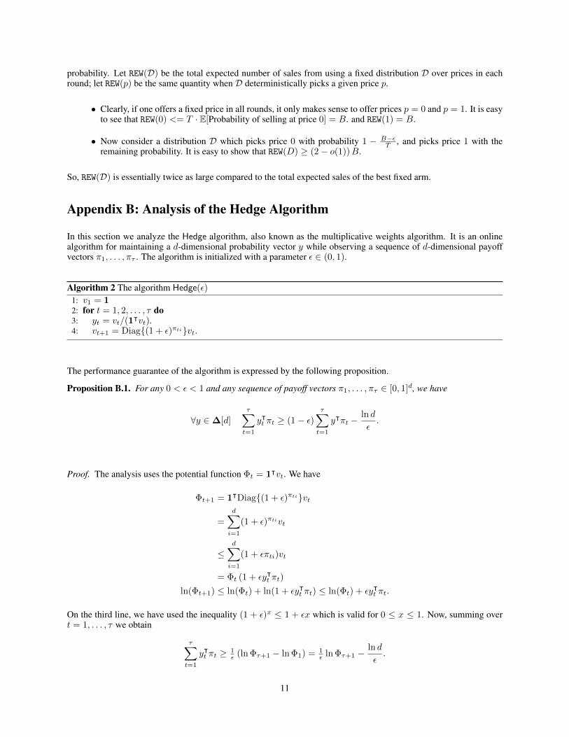
In this section we analyze the Hedge algorithm, also known as the multiplicative weights algorithm. It is an onlinealgorithm for maintaining a d-dimensional probability vector y while observing a sequence of d-dimensional payoffvectors π1, . . . , πτ . The algorithm is initialized with a parameter ε ∈ (0, 1).
Algorithm 2 The algorithm Hedge(ε)
1: v1 = 12: for t = 1, 2, . . . , τ do3: yt = vt/(1
ᵀvt).4: vt+1 = Diag(1 + ε)πtivt.
The performance guarantee of the algorithm is expressed by the following proposition.
Proposition B.1. For any 0 < ε < 1 and any sequence of payoff vectors π1, . . . , πτ ∈ [0, 1]d, we have
∀y ∈∆[d]
τ∑t=1
yᵀt πt ≥ (1− ε)τ∑t=1
yᵀπt −ln d
ε.
Proof. The analysis uses the potential function Φt = 1ᵀvt. We have
Φt+1 = 1ᵀDiag(1 + ε)πtivt
=
d∑i=1
(1 + ε)πtivt
≤d∑i=1
(1 + επti)vt
= Φt (1 + εyᵀt πt)
ln(Φt+1) ≤ ln(Φt) + ln(1 + εyᵀt πt) ≤ ln(Φt) + εyᵀt πt.
On the third line, we have used the inequality (1 + ε)x ≤ 1 + εx which is valid for 0 ≤ x ≤ 1. Now, summing overt = 1, . . . , τ we obtain
τ∑t=1
yᵀt πt ≥ 1ε (ln Φτ+1 − ln Φ1) = 1
ε ln Φτ+1 −ln d
ε.
11

The maximum of yᵀ (∑τt=1 πt) over y ∈∆[d] must be attained at one of the extreme points of ∆[d], which are simply
the standard basis vectors of Rd. Say that the maximum is attained at ei. Then we have
Φτ+1 = 1ᵀvτ+1 ≥ vτ+1,i = (1 + ε)π1i+···+πτi
ln Φτ+1 ≥ ln(1 + ε)
τ∑t=1
πti
τ∑t=1
yᵀt πt ≥ln(1 + ε)
ε
τ∑t=1
πti −ln d
ε
≥ (1− ε)τ∑t=1
yᵀπt −ln d
ε.
The last line follows from two observations. First, our choice of i ensures that∑τt=1 πti ≥
∑τt=1 y
ᵀπt for everyy ∈∆[d]. Second, the inequality ln(1 + ε) > ε− ε2 holds for every ε > 0. In fact,
− ln(1 + ε) = ln
(1
1 + ε
)= ln
(1− ε
1 + ε
)< − ε
1 + ε
ln(1 + ε) >ε
1 + ε>ε(1− ε2)
1 + ε= ε− ε2.
Appendix C: LP-optimal distributions over arms
We flesh out a claim about LP-optimal distributions, which we use for discretization (Section E.1).Claim C.1. For any latent structure µ, there exists a distributionD over arms which is LP-optimal for µ and moreoversatisfies the following three properties:
(a) ci(D, µ) ≤ B/T for each resource i.(b) D has a support of size at most d+ 1.(c) If D has a support of size at least 2 then for some resource i we have ci(D, µ) = B/T .
(Such distribution D will be called LP-perfect for µ.)
Proof. Fix the latent structure µ. It is a well-known fact that for any linear program there exists an optimal solutionwhose support has size that is exactly equal to the number of constraints that are tight for this solution. Take any suchoptimal solution ξ for linear program (P), and take the corresponding LP-optimal distribution D = ξ/‖ξ‖1. Sincethere are d + 1 constraints in (P), distribution D has support of size at most d + 1. If it satisfies property (a), we aredone. Note that such D also satisfies property (c).
Suppose property (a) does not hold for D. Then there exists a resource i such that ci(D, µ) > B/T . It follows that∑i ξi < T . Therefore, at most d constraints in (P) are tight for ξ, which implies that the support ofD has size at most
d.
Now, let us modify D to obtain another LP-optimal distribution D′ which satisfies both (a) and (b-c). Namely, letD′(x) = αD(x) for each non-null arm x, for some α ∈ (0, 1) that is sufficiently low to ensure property (a) (withequality for some resource i), and place the remaining probability in D′ on the null arm. Then LP(D′, µ) = LP(D, µ),so D′ is LP-optimal; D′ satisfies properties (a,c) by design, and it satisfies property (b) because it adds at most one tothe support of D.
Appendix D: Analysis of PD-BwK (Proof of Theorem 3.1)
In this section we present the analysis of the PD-BwK algorithm. We begin by recalling the Hedge algorithm fromonline learning theory, and its performance guarantee. Next, we present a simplified analysis of PD-BwK in a toymodel in which the outcome vectors are deterministic. (This toy model of the BwK problem is uninteresting as a
12

learning problem since the latent structure does not need to be learned, and the problem reduces to solving a linearprogram. We analyze PD-BwK first in this context because the analysis is simple, yet its main ideas carry over to thegeneral case which is more complicated.)
D.1 The Hedge algorithm
In this section we present the Hedge algorithm, also known as the multiplicative weights algorithm. It is an onlinealgorithm for maintaining a d-dimensional probability vector y while observing a sequence of d-dimensional payoffvectors π1, . . . , πτ . The algorithm is initialized with a parameter ε ∈ (0, 1).
Algorithm 3 The algorithm Hedge(ε)
1: v1 = 12: for t = 1, 2, . . . , τ do3: yt = vt/(1
ᵀvt).4: vt+1 = Diag(1 + ε)πtivt.
The Hedge algorithm is due to Freund and Schapire [20]. The version presented above, along with the followingperformance guarantee, are adapted from [26].Proposition D.1. For any 0 < ε < 1 and any sequence of payoff vectors π1, . . . , πτ ∈ [0, 1]d, we have
∀y ∈∆[d]
τ∑t=1
yᵀt πt ≥ (1− ε)τ∑t=1
yᵀπt −ln d
ε.
A self-contained proof of the proposition, for the reader’s convenience, appears in Appendix B.
D.2 Warm-up: The deterministic case
To present the application of Hedge to BwK in its purest form, we first present an algorithm for the case in whichthe rewards of the various arms are deterministically equal to the components of a vector r ∈ Rm, and the resourceconsumption vectors are deterministically equal to the columns of a matrix C ∈ Rd×m.
Algorithm 4 Algorithm PD-BwK, adapted for deterministic outcomes1: In the first m rounds, pull each arm once.2: Let r, C denote the reward vector and resource consumption matrix revealed in Step 1.3: v1 = 14: t = 15: for t = m+ 1, . . . , τ (i.e., until resource budget exhausted) do6: yt = vt/(1
ᵀvt).7: Pull arm xj such that point-mass distribution zt = ej belongs to argminz∈∆[X]
yᵀt Czrᵀz .
8: vt+1 = Diag(1 + ε)eᵀi Cztvt.
9: t = t+ 1.
This algorithm is an instance of the multiplicative-weights update method for solving packing linear programs. Inter-preting it through the lens of online learning, as in the survey [5], it is updating a vector y using the Hedge algorithm.The payoff vector in round t is given by Cxt. Note that these payoffs belong to [0, 1], by our assumption that C has[0, 1] entries.
Now let ξ∗ denote an optimal solution of the primal linear program (P) from Section 2.2, and let OPTLP = rᵀξ∗ denotethe optimal value of that LP. Let REW =
∑τ−1t=m+1 r
ᵀzt denote the total payoff obtained by the algorithm after itsstart-up phase (the first m rounds). By the stopping condition for the algorithm, we know there is a vector y ∈ ∆[R]such that yᵀC (
∑τt=1 zt) ≥ B so fix one such y. Note that the algorithm’s start-up phase consumes at most m units
of any resource, and the final round τ consumes at most one unit more, so
yᵀC
( ∑m<t<τ
zt
)≥ B −m− 1. (8)
13

Finally let
y =1
REW
∑m<t<τ
(rᵀzt)yt.
Now we have
B ≥ yᵀCξ∗ =1
REW
∑m<t<τ
(rᵀzt)(yᵀt Cξ
∗)
≥ 1
REW
∑m<t<τ
(rᵀξ∗)(yᵀt Czt)
≥ OPTLP
REW
[(1− ε)
∑m<t<τ
yᵀCzt −ln d
ε
]
≥ OPTLP
REW
[B − εB −m− 1− ln d
ε
].
The first inequality is by primal fesibility of ξ∗, the second is by the definition of zt, the third is the performanceguarantee of Hedge, the fourth is by (8). Putting these inequalities together we have derived
REW
OPTLP≥ 1− ε− m+ 1
B− ln d
εB.
Setting ε =√
ln dB we find that the algorithm’s regret is bounded above by OPTLP ·O
(√ln dB + m
B
).
D.3 Analysis modulo error terms
We now commence the analysis of Algorithm PD-BwK. In this section we show how to reduce the problem of boundingthe algorithm’s regret to a problem of estimating two error terms that reflect the difference between the algorithm’sconfidence-bound estimates of its own reward and resource consumption with the empirical values of these randomvariables. The analysis of those error terms will be the subject of Section D.4.
By Theorem 2.1 and our choice of Crad, it holds with probability at least 1 − T−1 that the confidence interval forevery latent parameter, in every round of execution, contains the true value of that latent parameter. We call this high-probability event a clean execution of PD-BwK. Our regret guarantee will hold deterministically assuming that a cleanexecution takes place. The regret can be at most T when a clean execution does not take place, and since this eventhas probability at most T−1 it contributes only O(1) to the regret. We will henceforth assume a clean execution ofPD-BwK.Claim D.2. In a clean execution of Algorithm PD-BwK, the algorithm’s total reward satisfies the bound
REW ≥ OPTLP −
[2OPTLP
(√ln d
B+m+ 1
B
)+m+ 1
]− OPTLP
B
∥∥∥∥∥ ∑m<t<τ
Etzt
∥∥∥∥∥∞
−
∣∣∣∣∣ ∑m<t<τ
δᵀt zt
∣∣∣∣∣ , (9)
where Et and δt are defined byEt = Ct − Lt, δt = ut − rt. (10)
Proof. The claim is proven by mimicking the analysis of Algorithm 4 in the preceding section, incorporating errorterms that reflect the differences between observable values and latent ones. As before, let ξ∗ denote an optimalsolution of the primal linear program (P), and let OPTLP = rᵀξ∗ denote the optimal value of that LP. Let REWUCB =∑m<t<τ u
ᵀt zt denote the total payoff the algorithm would have obtained, after its start-up phase, if the actual payoff
at time t were replaced with the upper confidence bound. By the stopping condition for the algorithm, we know thereis a vector y ∈∆[R] such that yᵀ (
∑τt=1 Ctzt) ≥ B, so fix one such y. As before,
yᵀ
( ∑m<t<τ
Ctzt
)≥ B −m− 1. (11)
Finally let
y =1
REWUCB
∑m<t<τ
(uᵀt zt)yt.
14

Assuming a clean execution, we have
B ≥ yᵀCξ∗ (ξ∗ is primal feasible)
=1
REWUCB
∑m<t<τ
(uᵀt zt)(yᵀt Cξ
∗)
≥ 1
REWUCB
∑m<t<τ
(uᵀt zt)(yᵀt Ltξ
∗) (clean execution)
≥ 1
REWUCB
∑m<t<τ
(uᵀt ξ∗)(yᵀt Ltzt) (definition of zt)
≥ 1
REWUCB
∑m<t<τ
(rᵀξ∗)(yᵀt Ltzt) (clean execution)
≥ OPTLP
REWUCB
[(1− ε)yᵀ
( ∑m<t<τ
Ltzt
)− ln d
ε
](Hedge guarantee)
=OPTLP
REWUCB
[(1− ε)yᵀ
( ∑m<t<τ
Ctzt
)− (1− ε)yᵀ
( ∑m<t<τ
Etzt
)− ln d
ε
]
≥ OPTLP
REWUCB
[(1− ε)B −m− 1− (1− ε)yᵀ
( ∑m<t<τ
Etzt
)− ln d
ε
](definition of y; see eq. (11))
REWUCB ≥ OPTLP
[1− ε− m+ 1
B− 1
B
∥∥∥∥∥ ∑m<t<τ
Etzt
∥∥∥∥∥∞
− ln d
εB
]. (12)
The algorithm’s actual payoff, REW =∑τt=1 r
ᵀt zt, satisfies the inequality
REW ≥ REWUCB −∑
m<t<τ
(ut − rt)ᵀzt = REWUCB −∑
m<t<τ
δᵀτ zt.
Combining this inequality with (12), we obtain the bound (9), as claimed.
D.4 Error analysis
In this section we complete the proof of Theorem 3.1 by deriving upper bounds on the terms∥∥∑
m<t<τ Etzt∥∥∞
and∣∣∑
m<t<τ δtzt∣∣ appearing on the right side of (9). Both bounds are special cases of a more general statement,
presented as Lemma D.4 below. Before stating the lemma, we need to establish a simple fact about confidence radii.Lemma D.3. For any two vectors a,N ∈ Rm+ , we have
m∑j=1
rad(aj , Nj)Nj ≤√Cradm(aᵀN) + Cradm. (13)
Proof. The definition of rad(·, ·) implies that rad(aj , Nj)Nj ≤√Crad ajNj + Crad. Summing these inequalities
and applying Cauchy-Schwarz,m∑j=1
rad(aj , Nj)Nj ≤m∑j=1
√Crad ajNj + Cradm ≤
√m ·
√∑j∈X
Crad ajNj + Cradm,
and the lemma follows by rewriting the expression on the right side.
The next lemma requires some notation and definitions. Suppose that a1, . . . , aτ is a sequence of vectors in [0, 1]m andthat z1, . . . , zτ is a sequence of vectors in e1, . . . , em. Assume that the latter sequence begins with a permutationof the elements of e1, . . . , em so that, for every s ≥ m, the diagonal matrix
∑st=1 ztz
ᵀt is invertible. The vector
as =
(s∑t=1
ztzᵀt
)−1( s∑t=1
ztzᵀt at
)
15
can be interpreted as the vector of empirical averages: the entry as,j is equal to the average of at,j over all times t ≤ ssuch that zt = ej . Let Ns =
∑st=1 zt denote the vector whose entry Ns,j indicates the number of times ej occurs in
the sequence z1, . . . , zs. A useful identity is
asᵀNt =
t∑s=1
aᵀszs.
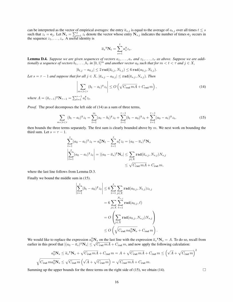
Lemma D.4. Suppose we are given sequences of vectors a1, . . . , aτ and z1, . . . , zτ as above. Suppose we are addi-tionally a sequence of vectors b1, . . . , bτ in [0, 1]m and another vector a0 such that for m < t < τ and j ∈ X ,
|bt,j − a0,j | ≤ 2 rad(at,j , Nt,j) ≤ 6 rad(a0,j , Nt,j).
Let s = τ − 1 and suppose that for all j ∈ X , |as,j − a0,j | ≤ rad(as,j , Ns,j). Then∣∣∣∣∣ ∑m<t<τ
(bt − at)ᵀzt
∣∣∣∣∣ ≤ O (√CradmA+ Cradm), (14)
where A = (aτ−1)ᵀNτ−1 =∑τ−1t=1 a
ᵀt zt.
Proof. The proof decomposes the left side of (14) as a sum of three terms,∑m<t<τ
(bt − at)ᵀzt =
m∑t=1
(at − bt)ᵀzt +
τ−1∑t=1
(bt − a0)ᵀzt +
τ−1∑t=1
(a0 − at)ᵀzt, (15)
then bounds the three terms separately. The first sum is clearly bounded above by m. We next work on bounding thethird sum. Let s = τ − 1.
s∑t=1
(a0 − at)ᵀzt = aᵀ0Nt −s∑t=1
aᵀt zt = (a0 − as)ᵀNs∣∣∣∣∣s∑t=1
(a0 − at)ᵀzt
∣∣∣∣∣ = |(a0 − as)ᵀNs| ≤∑j∈X
rad(as,j , Ns,j)Ns,j
≤√CradmA+ Cradm,
where the last line follows from Lemma D.3.
Finally we bound the middle sum in (15).∣∣∣∣∣s∑t=1
(bt − a0)ᵀzt
∣∣∣∣∣ ≤ 6
s∑t=1
∑j∈X
rad(a0,j , Nt,j)zt,j
= 6∑j∈X
Ns,j∑`=1
rad(a0,j , `)
= O
∑j∈X
rad(a0,j , Ns,j)Ns,j
≤ O
(√Crad na
ᵀ0Ns + Cradm
).
We would like to replace the expression aᵀ0Ns on the last line with the expression asᵀNs = A. To do so, recall fromearlier in this proof that |(a0 − as)ᵀNs| ≤
√CradmA+ Cradm, and now apply the following calculation:
aᵀ0Ns ≤ asᵀNs +√CradmA+ Cradm = A+
√CradmA+ Cradm ≤
(√A+
√Cradm
)2
√Cradma
ᵀ0Ns ≤
√Cradm
(√A+
√Cradm
)=√CradmA+ Cradm.
Summing up the upper bounds for the three terms on the right side of (15), we obtain (14).
16

Corollary D.5. In a clean execution of PD-BwK,∣∣∣∣∣ ∑m<t<τ
δtzt
∣∣∣∣∣ ≤ O (√CradmREW + Cradm)
and ∥∥∥∥∥ ∑m<t<τ
Etzt
∥∥∥∥∥∞
≤ O(√
CradmB + Cradm).
Proof. The first inequality is obtained by applying Lemma D.4 with vector sequences at = rt and bt = ut. The secondone is obtained by applying the same lemma with vector sequences at = eᵀ
i Ct and bt = eiLt, for each resource i.
Proof of Theorem 3.1: The theorem asserts that
REW ≥ OPT−O(√
m log(dmT )
(OPT√B
+√OPT +
√m log(dmT )
)).
Denote the right-hand side by f(OPT). The function maxf(x), 0 is a non-decreasing function of x, so to establishthe theorem we will prove that REW ≥ f(OPTLP) ≥ f(OPT), where the latter inequality is an immediate consequenceof the fact that OPTLP ≥ OPT (Lemma 2.3).
To prove REW ≥ f(OPTLP), we begin by recalling inequality (9) and observing that
2OPTLP
(√ln d
B+m+ 1
B
)= O
(√m log(dmT )
OPTLP√B
)by our assumption that m ≤ B. The term m+ 1 on the right side of Equation (9) is bounded above by m log(dmT ).Finally, using Corollary D.5 we see that the sum of the final two terms on the right side of (9) is bounded byO(√
Cradm(OPTLP√B
+√OPTLP +
√Cradm
)). The theorem follows by plugging in Crad = Θ(log(dmT )).
Appendix E: BwK with discretization
In this section we flesh out our approach to BwK with uniform discretization, as discussed in the Introduction. Thetechnical contribution here is a definition of the appropriate structure, and proof that discretization does not do muchdamage.Definition E.1. We say that arm x ε-covers arm y if the following two properties are satisfied for each resource i andevery latent structure µ in a given BwK domain:
(i) r(x, µ)/ci(x, µ) ≥ r(y, µ)/ci(y, µ)− ε.
(ii) ci(x, µ) ≥ ci(y, µ).
A subset S ⊂ X of arms is called an ε-discretization of X if each arm in X is ε-covered by some arm in S.
Note that we consider the difference in the ratio of expected reward to expected consumption, whereas for MAB inmetric spaces it suffices to consider the difference in expected rewards.
Once we construct an ε-discretization S of X , we can run a BwK algorithm on S and obtain expected total rewardcompetitive with OPTLP(S), the value of OPTLP if the action space is restricted to S. This makes sense if OPTLP(S) isnot much worse than OPTLP(X).Theorem E.2 (BwK: discretization). Fix a BwK domain with action spaceX . Consider an algorithmA which achievesexpected total reward REW ≥ OPTLP(S)−R(S) if applied to the restricted action space S ⊂ X , for any given S ⊂ X .If S is an ε-discretization of X , for some ε ≥ 0, then REW ≥ OPTLP − ε dB −R(S).
The main technical result here is that OPTLP(S) is not much worse than OPTLP(X). Such result is typically trivial inMAB settings where the benchmark is the best fixed arm, but requires some work in our setting because we need toconsider distributions over arms.
17

Lemma E.3. Consider an instance of BwK with action space X . Let S ⊂ X be an ε-discretization of X , for someε ≥ 0. Then OPTLP(S) ≥ OPTLP(X)− ε dB
Proof. Let D be the distribution over arms in X which maximizes LP(D, µ). We use D to construct a distribution DSover S which is nearly as good.
Let µ be the (actual) latent structure. For brevity, we will suppress µ from the notation: ci(x) = ci(x, µ) and ci(D) =ci(D, µ) for arms x, distributions D and resources i. Similarly, we will write r(x) = r(x, µ) and r(D) = r(D, µ).
We define DS as follows. Since S is an ε-discretization of X , there exists a family of subsets (cov(x) ⊂ X : x ∈ X)so that each arm x ε-covers all arms in cov(x), the subsets are disjoint, and their union is X . Fix one such family, anddefine
DS(x) =∑
y∈cov(x)
D(y) mini
ci(y)
ci(x), x ∈ S.
To argue that LP(DS , µ) is large, we upper-bound the resource consumption ci(DS), for each resource i, and lower-bound the reward r(DS).
ci(DS) =∑x∈S ci(x)DS(x)
≤∑x∈S
ci(x)∑
y∈cov(x)
D(y)ci(y)
ci(x)=∑x∈S
∑y∈cov(x)
D(y) ci(y) =∑y∈XD(y)ci(y)
= ci(D) (16)
(Note that the above argument did not use the properties (i-ii) in Definition E.1.)
r(DS) =∑x∈S r(x)DS(x)
=∑x∈S
r(x)∑
y∈cov(x)
D(y) mini
ci(y)
ci(x)
=∑x∈S
∑y∈cov(x)
D(y) mini
ci(y) r(x)
ci(x)
≥∑x∈S
∑y∈cov(x)
D(y) mini
r(y)− εci(y) (by Definition E.1(i))
=∑y∈X D(y) mini r(y)− εci(y)
≥∑y∈X D(y) (r(y)− ε
∑i ci(y))
= r(D)− ε∑i ci(D). (17)
Let τ(D) = miniB
ci(D) be the stopping time in the linear relaxation, so that LP(D, µ) = τ(D) r(D). By Equation (16)we have τ(DS) ≥ τ(D). We are ready for the final computation:
LP(DS , µ) = τ(DS) r(DS)
≥ τ(D) r(DS)
≥ τ(D) (r(D)− ε∑i ci(D)) (by Equation (17))
≥ r(D) τ(D)− ε τ(D)∑i ci(D)
≥ LP(D, µ)− ε dB.
E.1 Discretization for dynamic procurement
A little more work is needed to apply uniform discretization for dynamic procurement. Consider dynamic procurementwith non-unit supply. Throughout this subsection, assume n agents, budgetB, and ceiling Λ. Recall that in each roundt the algorithm makes an offer of the form (pt, λt), where pt ∈ [0, 1] is the posted price per unit, and λt ≤ Λ is themaximal number of units offered for sale in this round. The action space here is X = [0, 1]× 1 , . . . ,Λ, the set ofall possible (p, λ) pairs.
18

For each arm x = (p, λ), let S(x) be the expected number of items sold. Recall that expected consumption isc(x) = pS(x), and expected reward is S(x). It follows that r(x)
c(x) = 1p . By Definition E.1 price p ε-covers price q < p
if and only if 1p ≥
1q − ε.
It is easy to see that the hyperbolic ε-mesh S on [0, 1] is an ε-discretization: namely, each arm (q, λ) is ε-covered by(q, λ), where p is the smallest price in S such that p ≥ q. Unfortunately, such S has infinitely many points. In fact, it iseasy to see that any ε-discretization on X must be infinite (even for Λ = 1). To obtain a finite ε-discretization, we onlyconsider prices p ≥ p0, for some parameter p0 to be tuned later. We argue that this restriction is not too damaging.
We use a refinement of a notion of LP-optimal distribution over arms, see Appendix C.Claim E.4. Consider dynamic procurement with non-unit supply. Then for any p0 ∈ (0, 1) it holds that
OPTLP(0 ∪ [p0, 1]) ≥ OPTLP − Λ2p0n2/B.
Proof. When p0 > B/(nΛ) the bound is trivial and for the rest of the proof we assume that p0 ≤ B/(nΛ). Let D bethe distribution over arms which maximizes LP(D, µ) to get OPTLP. As proved in Appendix C, we can further assumethat D is LP-perfect. Thus, D has a support set of size at most 2, say arms xi = (pi, λi), i = 1, 2, where pi is theposted price and λi is the maximal allowed number of items. W.l.o.g. assume p1 ≤ p2. Note that p1 can be 0, whichwould correspond to the “null arm”. Moreover, letting si denote the expected number of items bought for arm (pi, λi),then by LP-perfectness the expected consumption is
c(D, µ) =∑2i=1D(xi) pisi ≤ B/n. (18)
(Formally, to apply Claim C.1 one needs to divide the rewards and consumptions (and hence the budget) by Λ, so thatconsumptions and rewards in each round are at most 1.)
Let us define a distribution D′ which has support in 0 ∪ [p0, 1].
• If p1 ≥ p0 then define D′ = D and we get OPTLP(0 ∪ [p0, 1]) ≥ OPTLP.
• From here on, assume p1 < p0. If D is a distribution of support 1 (i.e D′(x2) = 0) then defineD′(B/(nΛ), λ1) = 1 and we get OPTLP(0 ∪ [p0, 1]) ≥ OPTLP.
• If D is a distribution of support 2 then by LP-perfectness Equation (18) is satisfied with equality. Thereforep2 ≥ B/(ns2) ≥ B/(nΛ). Define
D′(p0, λ1) = D(p1, λ1)
D′(p2, λ2) = max(0,D(p2, λ2)− p0Λ
p2)
D′(0) = 1−D′(p0)−D′(p2).
Then D′ forms a feasible solution to the linear program (5), with support in 0 ∪ [p0, 1], and with valueLP(D′, µ) ≥ OPTLP − Λp0n/p2 ≥ OPTLP − Λ2p0n
2/B.
Let ALG be a BwK algorithm which achieves regret bound (1). Suppose ALG is applied to a discretized instanceof dynamic procurement, with m arms, n agents and budget B. For unit supply (Λ = 1), ALG has regretR(m,n,B) = O(
√mn + n
√m/B). For non-unit supply, in order to apply ALG we need to normalize the prob-
lem instance so that per-round rewards and consumptions are at most 1. That is, we need to divide all rewards, con-sumptions, and the budget, by the factor of Λ. Thus we obtain regret R(m,n,B/Λ) on the normalized instance, andtherefore regret ΛR(m,n,B/Λ) on the original problem instance. Using Lemma E.3 and Claim E.4 (and normalizing/ re-normalizing) we obtain the following regret bound:Corollary E.5. Consider dynamic procurement with non-unit supply. Fix ε, p0 ∈ (0, 1), and let S be the hyperbolicε-mesh on [p0, 1]. Then running ALG on arms S × 1 , . . . ,Λ achieves regret
ΛR(Λ|S|, n,B/Λ) + εB + p0 Λ2 n2/B.
Optimizing the parameters ε, p0 in Corollary E.5, we obtain the final regret bound.Theorem E.6. Consider dynamic procurement with non-unit supply. Assume n agents, budget B and ceiling Λ. LetALG be a BwK algorithm which achieves regret bound (1). Applying ALG with a suitably chosen discretization yieldsregret O(Λ3/2 n/B1/4).
19