bandwidth selection for weighted kernel density estimation · bandwidth selection for weighted...

arX

iv:0

709.

1616

v1 [

stat

.ME

] 1

1 Se

p 20

07

Electronic Journal of Statistics

Vol. 0 (0000)ISSN: 1935-7524

Bandwidth Selection for Weighted

Kernel Density Estimation

Bin Wang∗

Mathematics and Statistics Department,University of South Alabama,

Mobile, AL 36688e-mail: [email protected]

Xiaofeng Wang

The Cleveland Clinic,Cleveland, OH 44195

e-mail: [email protected]

Abstract: In the this paper, the authors propose to estimate the densityof a targeted population with a weighted kernel density estimator (wKDE)based on a weighted sample. Bandwidth selection for wKDE is discussed.Three mean integrated squared error based bandwidth estimators are in-troduced and their performance is illustrated via Monte Carlo simulation.The least-squares cross-validation method and the adaptive weight kerneldensity estimator are also studied. The authors also consider the boundaryproblem for interval bounded data and apply the new method to a realdata set subject to informative censoring.

Keywords and phrases: Biased Sampling, Informative Censoring, RightCensoring.

1. Introduction

Kernel-type density estimators are widely used due to their simple forms andsmoothness. Let X1, X2, . . .Xn be a set of data. A general class of density esti-mators can be defined as reweighted weight function estimators,

f(x) =

n∑

i=1

w(Xi)W (x,Xi), (1)

where W (.) is a weight function, which is usually taken to be a (symmetric)density function, and w(.) is a re-weighting function which can be adjusted tocontrol the roles of different data points in the sample. If we take

W (x, y) =1

hK

(

y − x

h

)

= Kh(y − x) and w(x) =1

n,

∗This project was supported in part by University of South Alabama Arts and SciencesSupport and Development award and Arts and Sciences Technological Infrastructure Enhance-ment award.

0

imsart-ejs ver. 2007/04/13 file: ejs_2007_112.tex date: October 25, 2018

http://arxiv.org/abs/0709.1616v1

http://www.i-journals.org/ejs

mailto:[email protected]

mailto:[email protected]

B. Wang and X. Wang/Bandwidth Selection for Weighted Kernel Density Estimation 1

we get a standard kernel density estimator,

f(x) =n∑

i=1

1

nhK

(

x−Xi

h

)

=n∑

i=1

1

nKh(x−Xi), (2)

where K(.) is a kernel function and h is the bandwidth which controls thesmooth of the estimate. Often the re-weighting function w(.) is required to benon-negative and sum up to 1. It can be a function of X itself and/or a vectorof covariates. For example, Gisbert used a function of the population of eachcountry to reweight the kernel density estimate of per capita GDP[8]. Marronand Padgett used a weighting function s, which is defined to be the jump sizesat X of the product-limit (PL) estimator by Kaplan and Meier[10], to correctthe random right-censoring bias (MP estimator hereafter). In the MP estimator,s is a function of both X and the censoring variable ∆, which is defined to be

∆(Xi) =

{

0, if Xi is censored,1, if Xi is not censored.

Thus, the bias induced by the random right-censoring can be corrected by thefollowing MP estimator,

fmp(x) =

n∑

i=1

siKh(x−Xi). (3)

Throughout this paper, the following general form of weighted kernel densityestimator will be used,

f(x) =

n∑

i=1

w(Xi, Zi)Kh(x−Xi). (4)

We simply choose K(.) to be a Gaussian kernel. For computational consider-ations, the Epanechnikov kernel can be used for large samples. Literature showsthat there is very little to choose between various kernels on the basis of meanintegrated square error. In this study, will focus on data with small or moderatesizes, so computation burden will not be a big issue.

The bandwidth selection problem has been well studied and documented forthe unweighted kernel density estimation. In Section 2 we will discuss the band-width selection problem for wKDE. Two rough estimators and a plug-in estima-tor of the optimal bandwidth are proposed. The least-squares cross-validationmethod will also be discussed to refine the three estimates from Section 2 andto automatically select the bandwidth. The adaptive wKDE and the boundaryproblem will be discussed in Session 3 and Section 4 respectively. In Section 5,we will introduce how to use wKDE to estimate densities from biased samplingand the performance of the proposed methods will be illustrated via simulationstudies in Section 6. Section 7 contains the results by applying the new methodto a real data set from literature. Section 8 concludes the paper with a briefsummary.



2. Bandwidth Selection

2.1. Two rough approaches

Bandwidth selection is one of the most important issues in kernel density es-timation. In this paper, we will select the bandwidth based on the mean in-

tegrated squared error (MISE) criteria. The MISE criteria was first proposedby Rosenblatt[17] and has been widely used for automatic bandwidth selection.

The MISE of f can be decomposed into a sum of an integrated square bias termand an integrated variance term as below,

MISE(f) =

∫

{Ef(x) − f(x)}2dx+

∫

varf(x)dx. (5)

If we take equal weights for all data points such that w(.) = 1/n in (4), theoptimal bandwidth minimizing the MISE is

hopt = k−2/52

{∫

K(t)2dt

}1/5 {∫

f ′′(x)2dx

}−1/5

n−1/5, (6)

where k2 =∫

t2K(t)dt [22]. However, with unequal weights, the expectation of

f(x) for each x is

Ef(x) =∑

E [w(Xi, Zi)Kh(x−Xi)] . (7)

The bias in (5), Ef(x)− f(x), can be rewritten as

biash(x) =

∫

w(y, z)n

hK

(

x− y

h

)

f(y)dy − f(x)

y=x−ht=

∫

nw(x − ht, z)K(t)f(x− ht)dt− f(x)

=

∫

K(t)[n · w(x − ht, z)f(x)− f(x)]dt (8)

−nhf ′(x)

∫

w(x − ht, z)tK(t)dt

+nh2

2f ′′(x)

∫

t2w(x − ht, z)K(t)dt

+O(h3).

If w(.) 6= 1/n, n · w(x − ht, z)f(x) − f(x) 6= 0, and the first term to the righthand side (RHS) of (8) won’t be zero. Also, although the Gaussian kernel is usedsuch that

∫

tK(t)dt = 0, after the Taylor series expansion, the integral part inthe second term to the RHS of (8) won’t be zero either, even if w(.) is free of

Z. Therefore, we can not rewrite the bias of f in form of the sum of a term oforder h2 and higher order terms as in [27, 22].



An easy and rough approximation is to expand and view the weighted sampleas an new unweighted sample. For instance, let X = {X1, X2, . . . , Xn} be theobserved survival data with random right-censoring. If Xi is censored, the truesurvival time of the ith individual is Ti ≥ Xi. Thus, we can view the censoredsurvival data as a data set consists of observed event times and latented truesurvival times, with the same size and all data points have equal weights. Thus,we can continue to use hopt in (6) to select the optimal bandwidth. We can findthat k2 and K(t) in (6) do not depend on the data. If n is kept unchanged,we need only figure out how to compute

∫

f ′′2 based on the weighted samplein computing hopt. For complete weighted data, n may be hard to determine,we will leave this problem for future studies. With additional assumptions, wepropose the following two rough approach of hopt.

Rough approach 1: In the same spirit of Parzen (1962) and Silverman(1986), we use a normal reference density to compute

∫

f ′′2 and approximatethe optimal bandwidth roughly by

hn = 0.9An−1/5, (9)

whereA = min(sw, IQRw/1.34).

We compute the weighted sample mean and sample variance by

µw =

n∑

i=1

w(Xi, Zi)Xi,

s2w =

n∑

i=1

w(Xi, Zi)(Xi − µw)2.

LetX(1), X(2), . . . X(n) be the order statistics ofX1, X2, . . . , Xn and w1, w2, . . . .wn

be the corresponding weights of the order statistics. We find two integers q1 andq2 such that

q1∑

i=1

wi ≤ .25 and

q1+1∑

i=1

wi > .25,

q2∑

i=1

wi ≤ .75 and

q2+1∑

i=1

wi > .75.

Let

p1 = .25−q1∑

i=1

wi and p2 = .75−q2∑

i=1

wi.

Based on the weighted sample, we can compute the first and third quartiles andIQRw by

Q1w = X(q1) + p1(X(q1+1) −X(q1)),

Q3w = X(q2) + p2(X(q2+1) −X(q2)),



andIQRw = Q3w −Q1w.

Rough approach 2: In survival data analysis, the exponential referencedensity is widely used in estimating

∫

f ′′2. Let

f(x) = 1/λ · exp(−x/λ),

We have∫

f ′′(x)2dx =1

λ6

∫

e−2x/λdx =1

2λ5. (10)

Plug-in (10) to (6), we get

hopt = π−1/10λn−1/5 = .892λn−1/5. (11)

The coefficient in (11) is close to 0.9 as in (9). We then get another roughestimate of the optimal bandwidth, he, by keeping the form of (9),

he = 0.9Bn−1/5, (12)

whereB = min(λ, IQRw/1.34),

and λ can be estimated by a maximum likelihood estimate λ =∑

Xi/∑

∆i for

the right-censored data and λ = X for the complete data.

2.2. Plug-in estimator

In addition to the normal and exponential reference densities, we can alsouse other reference densities. To be general, we mimic the plug-in method bySheather and Jones (1991) [20] to automatically select the bandwidth. A kernelbased estimate S(γ) will be used to estimate

∫

f ′′2 in (6),

S(γ) =1

(n− 1)γ5

n∑

i=1

n∑

j=1

wjK

(

Xi −Xj

γ

)

, (13)

which leads to an estimate of the plug-in bandwidth, hp, which is a solution of

S(γ) = (2√πh5n)−1, (14)

where

γ = 1.357{S(a)/T (b)}1/7h5/7,

T (b) =1

(n− 1)b7

n∑

i=1

n∑

j=1

wjK

(

Xi −Xj

b

)

,

a = 0.920IQRwn−1/7,

b = 0.912IQRwn−1/9.

The method of false position, which is a generalization of the Secant Method

[18], is used to find numerical solution of the root of h in (14).



2.3. Least-squares cross-validation

To select the bandwidth completely automatically, we apply the least-squarescross-validation (LSCV) method after we computed the bandwidth by (9) or(12). The LSCV optimal bandwidth will be found by finding an h in the nearbyregions of the rough estimate(s) that minimizes the intergrated square error

(ISE) of f ,

ISE(f) =

∫

(f − f)2 =

∫

f2 − 2

∫

ff +

∫

f2. (15)

Note that the third term to the right-hand-side does not depend on the data.So minimizing ISE in (15) is equivalent to minimizing the sum of the first two

terms. The first term can be computed by using f in (4). For simplicity, wedenote w(Xi, Zi) as wi and we have

∫

f(x)2dx =

∫

∑

i

wi

hK

(

x−Xi

h

)

×∑

j

wj

hK

(

x−Xj

h

)

dx

t=x/h=

1

h

∑

i

∑

j

wiwj

∫

K

(

Xi

h− t

)

K

(

t− Xj

h

)

dt.

The integral part is convolution of the kernel with itself. Due to the fact that theconvolution of two Gaussians is another Gaussian, by elementary manipulations,we obtain

∫

f(x)2dx =1√2h

∑

i

∑

j

wiwjK

(

Xi −Xj√2h

)

=∑

i

∑

j

wiwjK√2h(Xi −Xj).

The second term in (15) can be estimated by −2/n∑

f−i(Xi), where f−i isa Jackknife estimate which is constructed based on the data set by leaving thei-th point out of computing,

f−i(x) =

∑

j 6=i wjKh(x−Xj)∑

j 6=i wj. (16)

We can further simplify the second term by,

1

n

∑

i

f−i(Xi) =1

n

∑

i

[

∑

j 6=i wjKh(x −Xj)∑

j 6=i wj.

]

=1

n

∑

i

[

f(Xi)− wiKh(0)∑

j 6=i wj

]

=1

n

∑

i

[

f(Xi)− wi/√2π

∑

j 6=i wj

]

.



If all weights sum up to 1, we can compute∑

j 6=i wj by 1 − wi. However, forcensored survival data, the weights may not necessary be sum up to one. Herewe simply leave the denominator as is.

Thus, the LSCV optimal bandwidth, hlscv, can be found by minimizing

∑

i

∑

j

wiwjK√2h (Xi −Xj)−

2

n

∑

i

[

f(Xi)− wi/√2π

1− wi

]

. (17)

To find hlscv, we do the following grid search,

Step 1: First search on [hl, hu], where hl = 0.25h and hu = 1.5h, and his computed by either (9) or (12).Step 2: Second, expand the searching as below:

a. If the minimum occurred at the left edge, let h′u = hl + δ and h′

l =0.2h′

u and repeat the grid search in Step 1 over [h′l, h

′u]. The δ is an

increment in each step of searching. It should not be too small whenthe sample size is reasonably large due to that it will tremendouslyslow down the algorithm.

b. If the minimum occurred at the right edge, let h′l = hu − δ and

h′u = 5h′

l and repeat the grid search in Step 1.

c. If the minimum occurred not at the edge, let h′l = (hl + hmin)/2 and

h′u = (hu + hmin)/2 and repeat the grid search in Step 1.

Step 3: Repeat Step 1 and Step 2 for k times.

When we expand the searching in Step 2, we prefer that the new searchingrange, [h′

l, h′u], has a small overlap with the old one, [hl, hu], in case that hlscv

stays within [hl, hl + ǫ] or [hu − ǫ, hu] for small ǫ. As for how to select k, itdepends on the value of δ. We suggest a large k such as 5 or 6 and a large δ,say, δ = (hu − hl)/20. We need also take the sample size into consideration. Ifthe sample size is large, the optimal bandwidth tends to be small and we willprefer to adjust the coefficients in Step 2a and Step 2b such that the searchingwill be focused on the left side of the intervals; otherwise, on the right side.

3. Adaptive Weighted Kernel Density Estimator

One of the drawbacks of using a fixed bandwidth over the whole range of thesample data is that for long-tailed distributions that either the details wherethe data are dense will be masked or spurious noise will show in the tails.For weighted samples, the shape of the estimated density will be greatly af-fected by the weighting function. For example, the MP estimator will correctthe estimation bias in the following way: (1) all censored survival times will fi-nally be excluded from constructing the density estimate. (2) starting from thesmallest observed time, the weight of a censored data point ti will be equallyre-distributed to the data points with t > ti. As a result, the largest uncensored



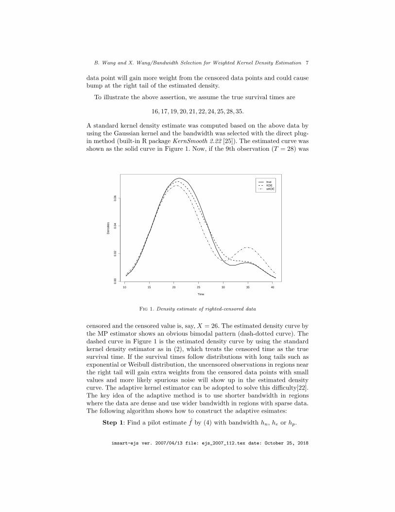
data point will gain more weight from the censored data points and could causebump at the right tail of the estimated density.

To illustrate the above assertion, we assume the true survival times are

16, 17, 19, 20, 21, 22, 24, 25, 28, 35.

A standard kernel density estimate was computed based on the above data byusing the Gaussian kernel and the bandwidth was selected with the direct plug-in method (built-in R package KernSmooth 2.22 [25]). The estimated curve wasshown as the solid curve in Figure 1. Now, if the 9th observation (T = 28) was

10 15 20 25 30 35 40

0.00

0.02

0.04

0.06

Time

Den

sitie

s

trueKDEwKDE

Fig 1. Density estimate of righted-censored data

censored and the censored value is, say, X = 26. The estimated density curve bythe MP estimator shows an obvious bimodal pattern (dash-dotted curve). Thedashed curve in Figure 1 is the estimated density curve by using the standardkernel density estimator as in (2), which treats the censored time as the truesurvival time. If the survival times follow distributions with long tails such asexponential or Weibull distribution, the uncensored observations in regions nearthe right tail will gain extra weights from the censored data points with smallvalues and more likely spurious noise will show up in the estimated densitycurve. The adaptive kernel estimator can be adopted to solve this difficulty[22].The key idea of the adaptive method is to use shorter bandwidth in regionswhere the data are dense and use wider bandwidth in regions with sparse data.The following algorithm shows how to construct the adaptive esimates:

Step 1: Find a pilot estimate f by (4) with bandwidth hn, he or hp.



Step 2: Define local bandwidth factor λi by

λi = {f(Xi)/g}−α, (18)

wherelog g = n−1

∑

log f(Xi)

and the sensitivity parameter α satisfies 0 ≤ α ≤ 1.Step 3: Define the adaptive kernel estimate f by

f(t) =

n∑

i=1

w(Xi, Zi)1

hλiK

(

t−Xi

hλi

)

. (19)

Literature shows that the pilot estimate in Step 1 is not that crucial[4, 1, 22].The performance of the adaptive wKDE and the choice of α will be studied viaMonte-Carlo method in Section 6.

4. Boundary Problem

It is often the case that the natural domain of definition of a density to beestimated is an interval bounded on one or two sides. In [8], the per capitaGDP mentioned above are measurements of positive quantities. In survival dataanalysis, the survival times will never be negative. There could also exist anupper bound in some other cases.

If there are not many observations near zero, one possible solution is tocalculate the estimate as if there is no restriction and then set f(x) to zero fornegative x. Normalizing can also be done to ensure the estimate integrate tounity. Another remedy is to do the log-transformation to the data on the half-line and compute the estimate, then transform back to the original scale. Thismethod could be useful, but the smoothness could be a potential problem: thesmoothness is guaranteed for the transformed data by selecting an appropriatebandwidth, but not for the data at the original scale. Sun and Wang[23] showedthat the transformation based kernel density estimate sometimes is less smoothfor the transformation Xt = g(X) = Xθ+1, where θ > 0.

Asymmetric kernels, such as inverse Gaussian, reciprocal inverse Gaussianand gamma-type kernels, were also considered to eliminate the difficulty of thekernel density estimation around the origin for censored data[5, 19, 12]. Mullerand Wang (1994) defined a class of boundary kernels and proposed to reducethe boundary effects by using boundary kernels in the boundary regions andvarying bandwidth under minimum mean squared errors criteria[15].

In this study, the reflection method and replication method is adopted tosolve the boundary problem[3]. By adding reflections of all points in the data,

we get a new data set {X1,−X1, X2,−X2, · · ·Xn,−Xn}. Let f ′ be the kernel



density estimate constructed based on the new data set. We can show that thedensity of the original data set can be computed by

f(x) =

{

2f ′(x), for x ≥ 0,0, for x < 0.

Of course we need not reflect all data points. Because a point stays 4σ away fromx will contribute very little to the density at x, we reflect points Xi ∈ [0, 4h)for i = 1, 2, . . . , n. The new weighted density estimator can be rewritten as

f(x) =

n∑

i=1

w(Xi, Zi) [Kh(x−Xi) +Kh(x+Xi) · I0≤x<4h] , (20)

where I(.) is an indication function.

5. Density Estimation from Biased Sampling

The wKDE can be used to estimate the densities based on biased samples. Inbiased sampling, if whether an element with X = x will be observed dependson its true value x, we obtain a biased sample. Let’s assume that Xi = xi, willbe sampled with probability b(xi). Let f(x) be the population density, we canshow that the density of the biased sample is a weighted version of f(x),

fs(x) = b(x)f(x)/κ, (21)

where κ is a normalizing constant such that

κ =

∫

b(x)f(x)dx.

Both b(.) and f(.) in (21) are non-parametrically identifiable if two or morerandom samples with overlaps are available [26]. However, based on just onesample, we need further restrictions on either b(.) or f(.) or both to ensure theidentifiability[24, 7]. Throughout this paper, we assume b(.) and further w(.) tobe parametrically known.

We can estimate fs(x) by a standard kernel density estimator as in (2) andtherefore obtain a natural estimate of f(x),

fb(x) = κfs(x)/b(x) =κ

n · b(x)

n∑

i=1

Kh(x−Xi). (22)

Wu (1997) proposed to estimate f(x) for s-dimension data by a kernel densityestimator [28]. We simply take s = 1 and get its univariate version estimate,

fwu(x) = κ′n∑

i=1

b−1(Xi)Kh(x−Xi), (23)



where κ′ = 1/∑

b(Xi).

Which estimate is better, fb(x) or fwu(x)? In (22), if the biasing function b(x)is coarse or not continuous, the estimate in (22) may also be coarse. While in(23), the estimate is smooth. A Monte Carlo study was carried out to comparetheir performance in density estimation based on biased samples. We first drew arandom sample, X , of size 200 from a targeted population; second, we mimickedthe biased sampling scheme by keeping observation X = x in the data set withprobability b(x); finally, we computed fb and fwu based on the biased samples.

To evaluate the performance, the L1 distance between f and f is computed,

L1(f, f) =

∫

|f − f | ≈m∑

i=1

|f(yi)− f(yi)| · di, (24)

where 0 ≤ y1 < y2 < . . . < ym and di = (yi+1 − yi−1)/2 for i = 2, 3, . . . ,m− 1and d1 = y2 − y1, dm = ym − ym−1.

We took two targeted populations: (a) Weibull distribution with shape pa-rameter 2 and scale parameter 1; and (b) normal distribution with mean 10and standard deviation 2. Two different biasing function were used for biasedsampling,

b1(x) ∝ x

b2(x) =

0.2 if x ≤ µ− 1.2σ,0.4 if µ− 1.2σ < x ≤ µ− 0.4σ,0.6 if µ− 0.4σ < x ≤ µ+ 0.4σ,0.8 if µ+ 0.4σ < x ≤ µ+ 1.2σ,1.0 if x > µ+ 1.2σ.

We repeated the above procedure for 10000 times for each setting and approx-imate the mean L1 distance and the standard error. The results are shown inTable 1. We find in all the four scenarios, fwu outperforms fb.

Table 1

Performance of wKDE and KDE for biased samples

N(10,2) Weibull(2,1)

b(.) f mean se mean se

b1(.) fb .130 4.37e-4 .167 6.51e-4

fwu .127 4.33e-4 .150 6.41e-4

b2(.) fb .194 4.43e-4 .221 5.80e-4

fwu .145 5.36e-4 .167 5.76e-4

In Figure 2, the Weibull distribution was used in plot (a) and (c), and thenormal distribution was used in plot (b) and (d). In Figure 2, the solid curvesshow the true density curves of f . The dashed curves and dotted curves representthe estimated density curves by fwu and fb respectively. In plot (a) and (b), we

find that when b(x) is smooth, both fb and fwu are smooth. The two estimators

work similarly well except that fb has a boundary problem due to that b(x) → 0when x → 0. The results in Table 1 also demostrate that the difference between



0.5 1.0 1.5 2.0

0.0

0.2

0.4

0.6

0.8

1.0

1.2

x

Den

sitie

s

(a) Weibull(2,1)

true ff.wu L1= 0.157f.b L1= 0.219

6 8 10 12 14

0.00

0.05

0.10

0.15

0.20

x

Den

sitie

s

(b) Normal(10,2)

true ff.wu L1= 0.157f.b L1= 0.219

0.5 1.0 1.5 2.0

0.0

0.2

0.4

0.6

0.8

1.0

1.2

x

Den

sitie

s

(c) Weibull(2,1)

true ff.wu L1= 0.157f.b L1= 0.219

6 8 10 12 14

0.00

0.05

0.10

0.15

0.20

x

Den

sitie

s

(d) Normal(10,2)

true ff.wu L1= 0.157f.b L1= 0.219

Fig 2. Kernel density estimate of length biased data

the two mean L1-distances of fb and fwu is not very large. However, in plot (c)

and (d), we can find that when the biasing function is a step function, fwu is

still smooth, but fb is not. The difference between the two mean L1-distancesalso becomes larger. In conclusion, fwu has better performance than fb.

6. Simulation

Simulation results will be presented in two parts. In part 1, we will illustratethe performance of hlscv and the adaptive bandwidths. In part 2, we will showthe performance of hn, he and hp.

6.1. Part 1: LSCV and Adaptive wKDE

Expereients were done to illustrate the performance of hlscv and the adaptivebandwidth. The following algorithm was used.

Step 1: draw a random sample from the targeted population;Step 2: compute hn and hp based on the sample;Step 3: search hlscv based on hn;



Step 4: compute the wKDEs with hn, hp and hlscv respectively and thecorresponding L1 distances.Step 5: take sensitivity parameter α = 0.3, 0.4, 0.5, 0.6, 0.7 and computethe pilot estimates of f by wKDE with hn, hlscv and hp respectively;compute the corresponding L1 distances.

We used two different population distributions: N(13, 32) and Weibull(2, 1) andtook different sample sizes n = 20, 30, 50, 100, 300. For each pair of n and f , theabove procedure was repeated for 10000 times and the mean and standard errorof the L1 distances were computed.

6.1.1. Complete Data

Simple random samples were drawn from N(13, 32). All data points in the sam-ples were equally weighted, under which all wKDE estimates reduce to thestandard kernel density estimate.

Table 2 shows the simulation results. The two values to the left are the mean

Table 2

Complete data from Normal distribution

Size hp awKDE hn awKDE hlscv awKDE20 .274 .277 .281 .288 .320 .315

(e-3) 1.143 1.180 1.111 1.142 1.611 1.66430 .235 .236 .232 .238 .273 .267

(e-3) .923 .955 .866 .892 1.276 1.33550 .194 .193 .192 .197 .225 .219

(e-3) .729 .746 .676 .692 .997 1.054100 .148 .147 .147 .151 .170 .166(e-3) .523 .528 .484 .492 .710 .754300 .097 .095 .097 .099 .108 .105(e-3) .306 .298 .282 .281 .403 .425

L1 distance of the wKDE by using either hp or hn or hlscv respectively (top)and its standard error (bottom). While the values to the right are those ofthe adaptive wKDE by using the corresponding bandwidth estimates. For eachsetting, only the best result for different α is displayed. In all cases, simulationresults suggest α = 0.3.

From Table 2, we find that the mean L1 distances and the standard errorsdecrease as n increases. The performance of hn and hp is similar: both outper-form hlscv. The adaptive wKDE improves the estimate for hlscv. For hn and hp,the adaptive wKDE does not improve the estimates. It improves the estimatefor hp a little bit when n is large, and makes the estimate worse for hn.

6.1.2. Incomplete Data

We drew random samples from both N(13, 32) and Weibull(2, 1), with 30% ofthe data points randomly right-censored. The weighting function w(.) is taken



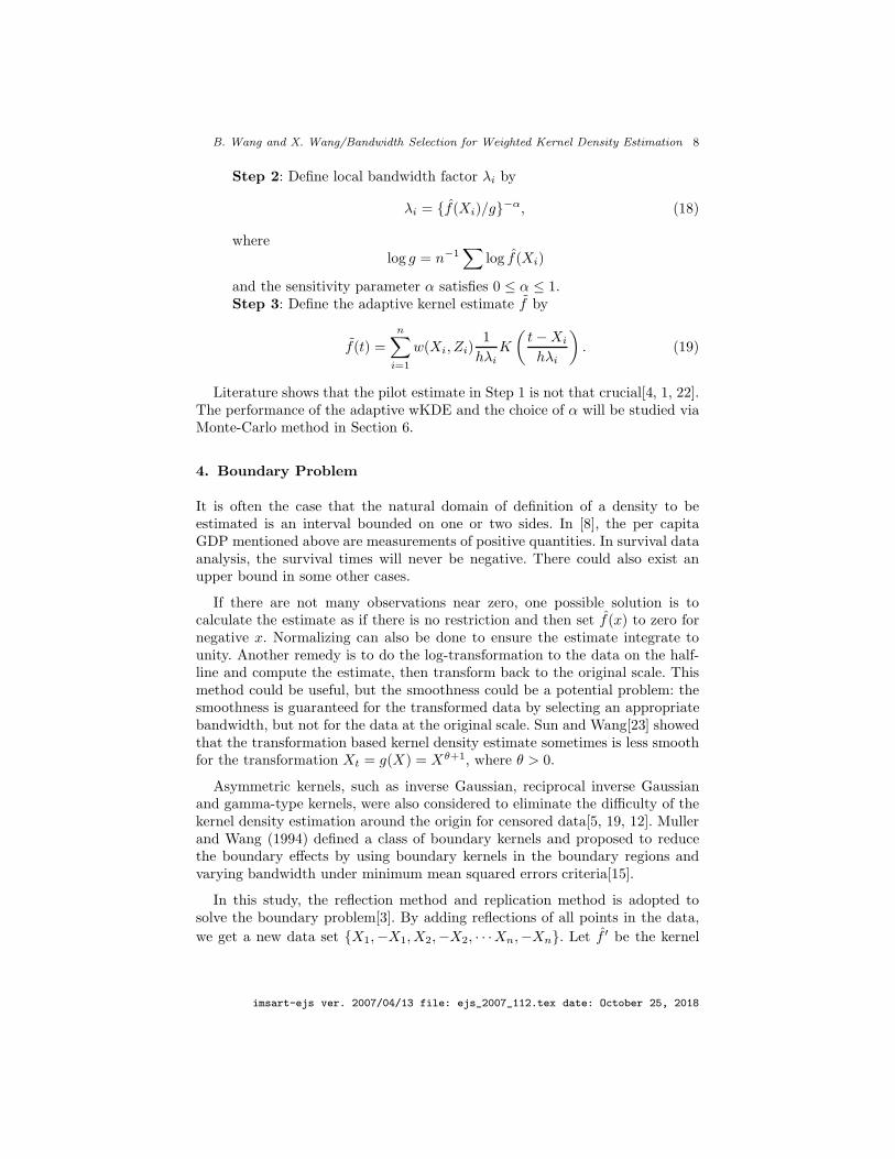
to be the jump sizes of the Kaplan-Meier estimator as MP estimator. Simulationresults are listed in Table 3 and Table 4. The sample sizes in the two tables are

Table 3

Incomplete data from Normal population


(e-3) 1.112 1.156 1.048 1.084 1.535 1.59340 .240 .242 .239 .245 .278 .272

(e-3) .964 1.005 .908 .942 1.320 1.38270 .197 .198 .196 .202 .226 .221

(e-3) .742 .763 .694 .716 1.004 1.055140 .156 .155 .156 .160 .177 .173(e-3) .551 .563 .517 .530 .717 .759300 .120 .121 .121 .125 .134 .132(e-3) .394 .399 .374 .379 .491 .522

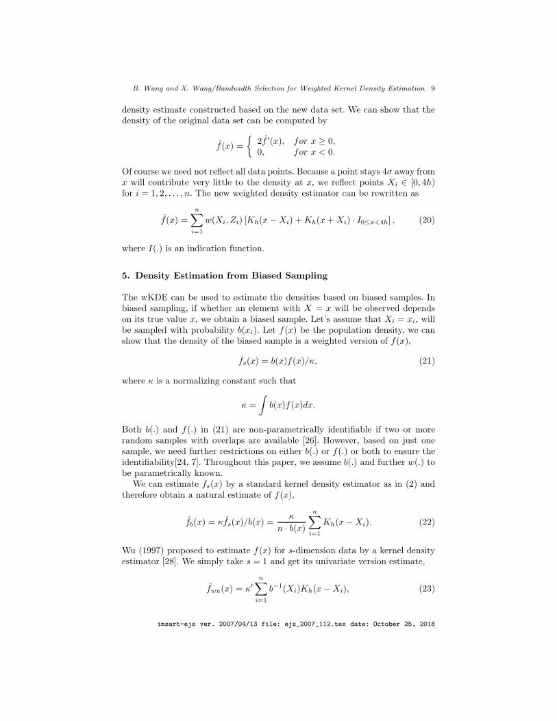
Table 4

Incomplete data from Weibull population


(e-3) 1.149 1.190 1.124 1.158 1.134 1.32440 .269 .272 .268 .273 .398 .397

(e-3) .993 1.025 .985 1.011 1.298 1.26270 .230 .231 .229 .232 .373 .371

(e-3) .797 .811 .790 .800 1.266 1.212140 .194 .194 .193 .194 .353 .347(e-3) .606 .609 .603 .605 1.339 1.280300 .168 .168 .166 .167 .330 .323(e-3) .465 .460 .462 .459 1.471 1.413

the sizes of the original data before censoring. We took larger sample sizes suchthat we had approximately the same amount of uncensored data points, as inTable 2, in computing the kernel density estimates. We can find that hlscv doesnot work as well as hn and hp for data from both populations. The adaptivemethod improves the estimate with hlscv, but not those with hp and hn.

Remarks: (a) The hlscv does not work well. This is consistent to the conclu-sion in [2], where Altman and Leger suggested plug-in estimator instead of usingleave-one-out or leave-some-out method to seek optimal bandwidth. For right-censored data, the reweighting scheme will compromise the sparseness of dataat the right tail and the adaptive method won’t work as well as expected. (b)The rough approach hn outperforms the other two methods (in some settings,its performance is very similar to hp).

6.2. Part 2: Performance of hn, he and hp

In this part, we studied the performance of hn, he and hp by comparing withan existing estimator by Kuhn and Padgett (1997, KP estimator hereafter)[11].The KP estimator is an estimator proposed for survival data subject to random



right-censoring which selects the bandwidth locally by minimizing a mean ab-solute error, which is supposed to be more nature than the mean squared errorcriteria [6]. The optimal bandwidth used by KP estimator is

hkp(x) =

{

4α2f(x)R(K)

nµ22f

′′(x)2H∗(x)

}1/5

, (25)

where α = 0.4809489. When a Gaussian kernel is used, we have R(K) =(2√π)−1 and µ2

2 = 1. The censoring survival function, H∗(x), is estimatedby the product-limit (PL) estimator, H∗(x) = 1− H(x), where

H(x) =

1, 0 ≤ x ≤ X(1),∏k−1

i=1

(

n−in−i+1

)1−∆i

, X(k−1) < x ≤ X(k), k = 2, · · · , n,0, x > X(n).

Here X(1), · · · , X(n) are the order statistics of X1, · · · , Xn. An exponential refer-ence density, fR(x) = λ−1 exp(−x/λ), is preferred, where λ is estimated by themaximum likelihood estimate

λ =

∑ni=1 Xi

∑ni=1 ∆i

.

Thus we have

hkp(x) = 0.7644174 · λH∗(x)−1/5ex/5λn−1/5 (26)

and we can express the KP estimate by

fkp(x) =

n∑

i=1

∆i

nH∗(Xi)Khkp(Xi)

(

x−Xi

hkp(Xi)

)

. (27)

Random samples were drawn from three different distributions: (a) normaldistribution with mean 13 and variance 9, (b) exponential distribution withmean 1, and (c) Weibull distribution with shape parameter 2 and scale param-eter 1. For each sample, approximately 30% of the data points were randomlyright-censored. Based on the censored data together with the censoring informa-tion (∆), we estimated the density by wKDE with different bandwidths hn, he,hp and hkp respectively. The L1 distances were computed and shown in Table 5through Table 7 together with the corresponding standard errors.

From Table 5, it can be found that hn, he and hp all work well for censoreddata from the normal population, while hp outperforms the other three methods.The estimator hn has a relatively larger mean L1 distances and the smalleststandard errors. The KP estimator does not work well. This may be due to thefact that we used a normal density while KP estimator assume an exponentialreference density. Though, the performance of he was not affected much becausewe took the minimum of sw and IQRw/1.34 in (12). As shown in Table 6,



Table 5

N(13, 32)

Size hkp hn he hp

30 .741 .283 .276 .267(e-3) .590 1.076 1.105 1.09550 .710 .234 .230 .224

(e-3) .501 .828 .845 .887100 .654 .180 .178 .175(e-3) .381 .601 .607 .665200 .586 .143 .142 .139(e-3) .284 .442 .445 .492

Table 6

Exponential(1)

Size hkp hn he hp

30 .263 .335 .334 .382(e-3) 1.200 1.287 1.291 1.20750 .243 .301 .301 .345

(e-3) 1.004 1.032 1.037 .941100 .223 .264 .264 .302(e-3) .793 .777 .779 .704200 .207 .236 .237 .267(e-3) .614 .592 .590 .532

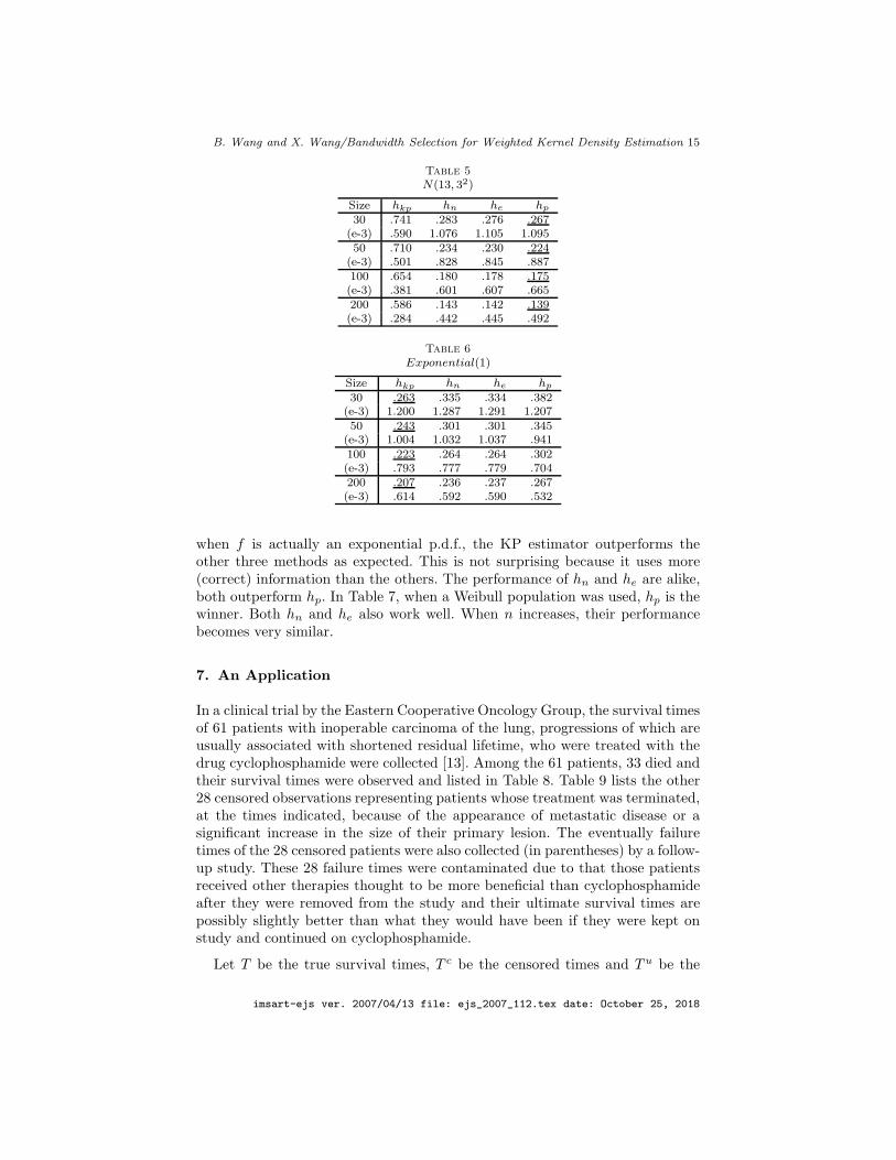
when f is actually an exponential p.d.f., the KP estimator outperforms theother three methods as expected. This is not surprising because it uses more(correct) information than the others. The performance of hn and he are alike,both outperform hp. In Table 7, when a Weibull population was used, hp is thewinner. Both hn and he also work well. When n increases, their performancebecomes very similar.

7. An Application

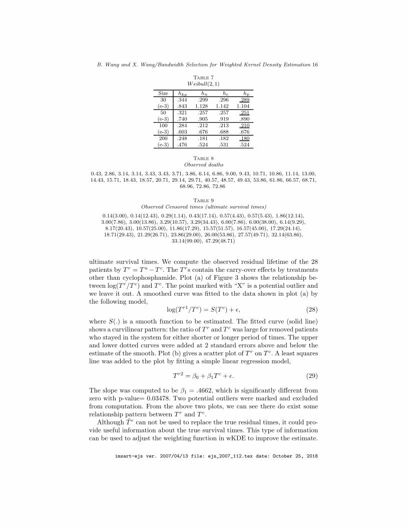
In a clinical trial by the Eastern Cooperative Oncology Group, the survival timesof 61 patients with inoperable carcinoma of the lung, progressions of which areusually associated with shortened residual lifetime, who were treated with thedrug cyclophosphamide were collected [13]. Among the 61 patients, 33 died andtheir survival times were observed and listed in Table 8. Table 9 lists the other28 censored observations representing patients whose treatment was terminated,at the times indicated, because of the appearance of metastatic disease or asignificant increase in the size of their primary lesion. The eventually failuretimes of the 28 censored patients were also collected (in parentheses) by a follow-up study. These 28 failure times were contaminated due to that those patientsreceived other therapies thought to be more beneficial than cyclophosphamideafter they were removed from the study and their ultimate survival times arepossibly slightly better than what they would have been if they were kept onstudy and continued on cyclophosphamide.

Let T be the true survival times, T c be the censored times and T u be the



Table 7

Weibull(2,1)

Size hkp hn he hp

30 .344 .299 .296 .289(e-3) .843 1.128 1.142 1.10450 .321 .257 .257 .251

(e-3) .740 .905 .919 .890100 .284 .212 .213 .210(e-3) .603 .676 .688 .676200 .248 .181 .182 .180(e-3) .476 .524 .531 .524

Table 8

Observed deaths

0.43, 2.86, 3.14, 3.14, 3.43, 3.43, 3.71, 3.86, 6.14, 6.86, 9.00, 9.43, 10.71, 10.86, 11.14, 13.00,14.43, 15.71, 18.43, 18.57, 20.71, 29.14, 29.71, 40.57, 48.57, 49.43, 53.86, 61.86, 66.57, 68.71,

68.96, 72.86, 72.86

Table 9

Observed Censored times (ultimate survival times)

0.14(3.00), 0.14(12.43), 0.29(1.14), 0.43(17.14), 0.57(4.43), 0.57(5.43), 1.86(12.14),3.00(7.86), 3.00(13.86), 3.29(10.57), 3.29(34.43), 6.00(7.86), 6.00(38.00), 6.14(9.29),8.17(20.43), 10.57(25.00), 11.86(17.29), 15.57(51.57), 16.57(45.00), 17.29(24.14),18.71(29.43), 21.29(26.71), 23.86(29.00), 26.00(53.86), 27.57(49.71), 32.14(63.86),

33.14(99.00), 47.29(48.71)

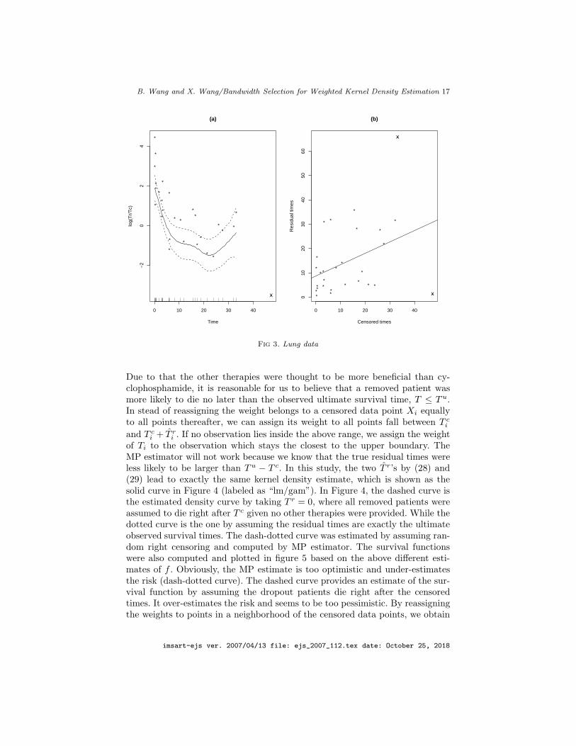
ultimate survival times. We compute the observed residual lifetime of the 28patients by T r = T u−T c. The T rs contain the carry-over effects by treatmentsother than cyclophosphamide. Plot (a) of Figure 3 shows the relationship be-tween log(T r/T c) and T c. The point marked with “X” is a potential outlier andwe leave it out. A smoothed curve was fitted to the data shown in plot (a) bythe following model,

log(T r1/T c) = S(T c) + ǫ, (28)

where S(.) is a smooth function to be estimated. The fitted curve (solid line)shows a curvilinear pattern: the ratio of T r and T c was large for removed patientswho stayed in the system for either shorter or longer period of times. The upperand lower dotted curves were added at 2 standard errors above and below theestimate of the smooth. Plot (b) gives a scatter plot of T r on T c. A least squaresline was added to the plot by fitting a simple linear regression model,

T r2 = β0 + β1Tc + ǫ. (29)

The slope was computed to be β1 = .4662, which is significantly different fromzero with p-value= 0.03478. Two potential outliers were marked and excludedfrom computation. From the above two plots, we can see there do exist somerelationship pattern between T r and T c.

Although T r can not be used to replace the true residual times, it could pro-vide useful information about the true survival times. This type of informationcan be used to adjust the weighting function in wKDE to improve the estimate.



0 10 20 30 40

−2

02

4

Time

log(

Tr/

Tc)

*

*

*

*

**

*

*

*

*

*

*

*

*

* *

*

**

*

*

**

**

*

*

*X

(a)

*

*

*

*

**

*

*

*

*

*

*

*

*

**

*

*

*

*

*

* *

*

*

*

*

*

0 10 20 30 40

010

2030

4050

60

Censored times

Res

idua

l tim

es

X

X

(b)

Fig 3. Lung data

Due to that the other therapies were thought to be more beneficial than cy-clophosphamide, it is reasonable for us to believe that a removed patient wasmore likely to die no later than the observed ultimate survival time, T ≤ T u.In stead of reassigning the weight belongs to a censored data point Xi equallyto all points thereafter, we can assign its weight to all points fall between T c

i

and T ci + T r

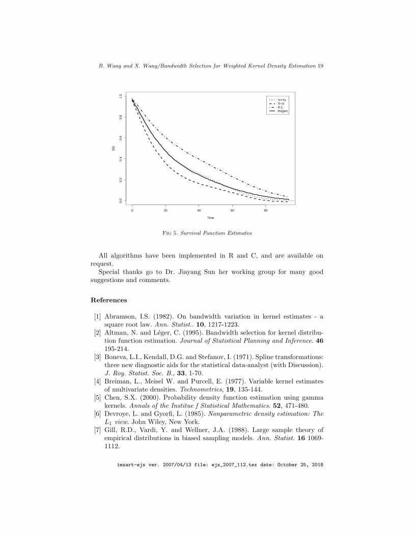
i . If no observation lies inside the above range, we assign the weightof Ti to the observation which stays the closest to the upper boundary. TheMP estimator will not work because we know that the true residual times wereless likely to be larger than T u − T c. In this study, the two T r’s by (28) and(29) lead to exactly the same kernel density estimate, which is shown as thesolid curve in Figure 4 (labeled as “lm/gam”). In Figure 4, the dashed curve isthe estimated density curve by taking T r = 0, where all removed patients wereassumed to die right after T c given no other therapies were provided. While thedotted curve is the one by assuming the residual times are exactly the ultimateobserved survival times. The dash-dotted curve was estimated by assuming ran-dom right censoring and computed by MP estimator. The survival functionswere also computed and plotted in figure 5 based on the above different esti-mates of f . Obviously, the MP estimate is too optimistic and under-estimatesthe risk (dash-dotted curve). The dashed curve provides an estimate of the sur-vival function by assuming the dropout patients die right after the censoredtimes. It over-estimates the risk and seems to be too pessimistic. By reassigningthe weights to points in a neighborhood of the censored data points, we obtain



0 20 40 60 80

0.00

00.

005

0.01

00.

015

0.02

00.

025

0.03

0

Time

Den

sitie

s

Tr=TuTr=0R.C.lm/gam

Tr=0lm/gam

R.C.

R.C.

Tr=Tu

Fig 4. Density estimates

the survival function as the solid curve in figure 5. This curve is very close tothe one by assuming the true survival times are the ultimate survival times.

8. Summary

In summary, the two rough approaches and the plug-in method work well inbandwidth selection for wKDE. If the target distribution is a exponential-likedistribution, the KP estimator is also a good choice. The LSCV method and theadaptive estimator won’t improve the estimate for wKDE. For large samples,Fourier transform or fast Fourier transform and kernels such as Epanechnikovkernel can be considered, which could remarkably improve the computationalspeed [14, 21, 9].

By choosing an appropriate weighting function, the wKDE can be used torobustly and efficiently estimate the densities from survival data subject to ran-dom censoring. The situation for data subject to informative censoring is muchcomplicated, because the it’s hard to model the sampling scheme. A possiblesolution is try to classify the censored data points into several categories and usethe prior information we have to define different weight-redistribution schemes,and finally apply wKDE to estimate the density. Alternatively, instead of as-signing weights to values after the censoring times equally or only to points incertain neighborhoods, we can also consider impute the censored times and re-assign weights to points in the nearby regions. When covariates are available, aparametric model or quantile regression could be more efficient. Further studieswill be carried out and the results will be presented in another research paper.



0 20 40 60 80

0.0

0.2

0.4

0.6

0.8

1.0

Time

S(t

)

Tr=TuTr=0R.C.lm/gam

Fig 5. Survival Function Estimates

All algorithms have been implemented in R and C, and are available onrequest.

Special thanks go to Dr. Jiayang Sun her working group for many goodsuggestions and comments.

References

[1] Abramson, I.S. (1982). On bandwidth variation in kernel estimates - asquare root law. Ann. Statist.. 10, 1217-1223.

[2] Altman, N. and Leger, C. (1995). Bandwidth selection for kernel distribu-tion function estimation. Journal of Statistical Planning and Inference. 46195-214.

[3] Boneva, L.I., Kendall, D.G. and Stefanov, I. (1971). Spline transformations:three new diagnostic aids for the statistical data-analyst (with Discussion).J. Roy. Statist. Soc. B., 33, 1-70.

[4] Breiman, L., Meisel W. and Purcell, E. (1977). Variable kernel estimatesof multivariate densities. Technometrics, 19, 135-144.

[5] Chen, S.X. (2000). Probability density function estimation using gammakernels. Annals of the Institue f Statistical Mathematics. 52, 471-480.

[6] Devroye, L. and Gyorfi, L. (1985). Nonparametric density estimation: The

L1 view. John Wiley, New York.[7] Gill, R.D., Vardi, Y. and Wellner, J.A. (1988). Large sample theory of

empirical distributions in biased sampling models. Ann. Statist. 16 1069-1112.



[8] Gisbert, Francisco J. Goerlich, (2003). Weighted samples, kernel densityestimators and convergence. Empirical Economics. 28, 335-351.

[9] Jones, M.C. and Lotwick, H.W. (1984). A remark on Algorithm AS 176.Kernel density estimation using the fast Fourier transform. Remark ASR50. Appl. Statist. 33, 120-122.

[10] Kaplan, E.L. and Meier, P. (1958). Nonparametric estimation from incom-plete observation. J. Amer. Statist. Assoc. 53 457-481.

[11] Kuhn, J.W. and Padgett, W.J. (1997). Local bandwidth selection for kerneldensity estimation from right-censored data based on asymptotic meanabsolute error. Nonlinear Analysis, Thoery, Methods & Applications, 30

4375-4384.[12] Kulasekera, K.B. and Padgett, W.J. (2006). Bayes bandwidth selection in

kernel density estimation with censored data. Nonparametric Statistics.18 129-143.

[13] Lagakos, S.W. (1979). General right censoring and its impact on the anal-ysis of survival data. Biometrics. 35, 139-156.

[14] Monro, D.M. (1976). Real discrete fast Fourier transform. Statistical Algo-rithm AS 97. Appl. Statist. 25, 166-172.

[15] Muller, H.G. and Wang, J.L. (1994) Hazard rate esimation under randomcensoring with varying kernels and bandwidths. Biometrics 50. 61-76.

[16] Parzen, E. (1962). On estimation of a probability density function andmode. Ann. Math. Statist. 33 1065-1076.

[17] Rosenblatt, M. (1956) Remarks on some nonparametric estimates of a den-sity function. Ann. Math. Statist. 27 832-837.

[18] Sauer, T. (2006). Numerical Analysis. Pearson Addison-Wesley.[19] Scaillet, O. (2004). Density estimation using inverse and reciprocal inverse

Gaussian kernels .Journal of Nonparametric Statistics. 16 217-266[20] Sheather, S. J. and Jones, M. C. (1991). A reliable data-based bandwidth

selection method for kernel density estimation. Journal of the Royal Sta-

tistical Society, Series B, 53, 683-690.[21] Silverman, B.W. (1982). Kernel density estimation using the fast Fourier

transform Statistical Algorithm AS 176. Appl. Satist. 31, 93-97.[22] Silverman, B. W. (1986) Density Estimation for Statistics and Data Analy-

sis. Chapman and Hall. Monographs on Statistics and Applied Probability.London.

[23] Sun, J. and Wang, B. (2006) Sieve estimates for biased survival data. IMS

Lecture Notes-Monograph Series: Recent Development in Nonparametric

Inference and Probability. 50 127-143.[24] Vardi, Y. (1985). Empirical distributions in selection bias models (with

discussions). Ann. Statist. 13 178-205.[25] Wand, M.P. and Jones, M.C. (1995).Kernel Smoothing. Chapman and Hall,

London.[26] Wang, B. and Sun, J. (2007) Inferences from biased samples with a memory

effect. Journal of Statistical planning and inference. (submitted).[27] Whittle, P. (1958). On the smoothing of probability density functions. J.

Roy. Statist. Soc. B., 20, 334-343.



[28] Wu. C. O. (1997). A cross-validation bandwidth choice for kernel densityestimates with selection biased data. Journal of multivariate analysis. 6138-60.


bandwidth selection for weighted kernel density estimation · bandwidth selection for weighted...

Documents